Fast Computational Methods for Visually Guided Robots∗

Maryam Mahdaviani, Nando de Freitas, Bob Fraser and Firas HamzeComputer Science DepartmentUniversity of British Columbia

{maryam,nando,robertf,fhamze}@cs.ubc.ca

Abstract— This paper proposes numerical algorithms forreducing the computational cost of semi-supervised and activelearning procedures for visually guided mobile robots fromO(M3) to O(M), while reducing the storage requirementsfrom M2 to M . This reduction in cost is essential forreal-time interaction with mobile robots. The considerablespeed ups are achieved using Krylov subspace methods andthe fast Gauss transform. Although these state-of-the-artnumerical algorithms are known, their application to semi-supervised learning, active learning and mobile robotics isnew and should be of interest and great value to the roboticscommunity. We apply our fast algorithms to interactive objectrecognition on Sony’s ERS-7 Aibo. We provide comparisonsthat clearly demonstrate remarkable improvements in com-putational speed.

Index Terms— Visually guided mobile robots, interactiverobots, learning, Krylov subspace methods, fast Gauss trans-form.

I. INTRODUCTION

Fig. 1. Aibo is an interactive robot that learns to recognize objectsusing semi-supervised input from a portable computer. Aibo alsouses active learning to prompt the user for labels. In the imagewe see Aibo correctly identifying the ball and the banana.

In this paper, we introduce fast algorithms for semi-supervised and active learning in visually guided robots[17], [18]. These algorithms make it possible to applythese computationally intensive learning tools in interactiverobotics. In particular, they reduce the computational costof learning from O(M3) to O(M) and the storage require-ments from M2 to M , where M is the number of features.Our application involves an ERS-7 Aibo that learns basicobject discriminants using semi-supervised input from the

∗This work is supported by NSERC and IRIS-ROPAR.

user, as shown in Fig. 1. That is, the user provides labelsfor some of the image regions observed by Aibo. Aibothen labels the rest of the image regions as well as all newimages in its video input. In this fashion, the user teachesAibo to recognize multiple objects.

When Aibo is confused about the label of an object, itemploys the active learning algorithms [18] to prompt theuser for new labels. Initially, a simple interface is used toteach Aibo to recognize a few objects in its environment.Subsequently, Aibo “asks questions” only when it “thinks”the answers could improve its recognition performance sig-nificantly within a Bayesian decision theoretic framework.This application allows humans to train visually guidedentertainment robots in a fun and interactive way thatplaces minimal burden on the human teacher. After learn-ing to recognize several objects in its environment, Aibocan use some of these objects as navigation landmarks.Conceivably, it can also use the recognition models andalgorithms to carry out simple tasks, such as fetching balls.

II. SEMI-SUPERVISED AND ACTIVE LEARNING USINGGAUSSIAN FIELDS

We begin with a description of the semi-supervisedlearning problem and the solution proposed in [17]. Weare given N feature vectors x ∈ R

d as shown for d = 2 inFig. 2. Some of the points have labels. In the figure, twopoints have the labels yl = 1 and yl = 0. The rest of thepoints have unknown labels yu. The goal is to compute theunknown labels.

x

wi

ij

j

x

Fig. 2. Input data. Two points (×) and (o) have labels yl = 1and yl = 0 respectively. The remaining points are unlabelledyu =?, but their topology is essential to the construction of agood classifier.

A human would classify all the points in the outer ringas 1 and the points in the inner circle as 0. We want analgorithm that reproduces this perceptual grouping. We dothis by considering each point xi as a node in a fully

connected undirected graph. The edges of the graph haveweights corresponding to a similarity kernel. In our case,the weight between points xi and xj is

wij = exp

(− 1

σ‖xi − xj‖2

),

where ‖ · ‖ denotes the L2 norm. Hence, points that areclose together will have high similarity (high w), whereaspoints that are far apart will have low similarity.

It is sensible to minimize the following error function tocompute the unknown labels yu:

E(yu) =1

2

∑

i∈L,j∈L

wij(yli − yl

j)2 + 2

∑

i∈U,j∈L

wij(yui − yl

j)2

+∑

i∈U,j∈U

wij(yui − yu

j )2

,

where L is the set of labelled points and U is the set ofunlabelled points. If two points are close then w will belarge. Hence, the only way to minimize the error functionis to make these two nearby points have the same label y.Let us introduce the adjacency matrix W with entries wij

and let D = diag(di) where di =∑

j wij . That is, D isa diagonal matrix whose i-th diagonal entry is the sum ofthe entries of row i of W. Let the vector yu contain allthe unknown labels yu and similarly let yl contain all thelabels yl. Then, the error function can be written in matrixnotation as follows:

E(yu)= yTu (Duu−Wuu)yu−2yT

l Wulyu+yTl (Dll−Wll)yl,

where Wuu denotes the entries wij with i, j ∈ U . Differ-entiating this error function and equating to zero, gives usour solution in terms of a linear system of equations:

(Duu − Wuu)yu = Wulyl, (1)

where 0 ≤ yu ≤ 1. A naive solution would cost O(M 3),where M = |U | is the number of unlabelled points, since|L| is significantly smaller than |U |.

Once we have labels for all N points in the training data,a new point xk in the test set data is classified using thefollowing classical kernel discriminant

yk =

∑N

i=1 wikyi∑N

i=1 wik

. (2)

As shown in [18], one can use Bayesian decision theoryto extend this semi-supervised learning approach to theactive learning domain. In this approach, the class pos-terior probabilities p(yu

i |yl,x) are approximated with theestimates 0 ≤ yu

i ≤ 1, yielding the following expressionfor the posterior risk of the Bayes classifier:

R(yu) =

M∑

i=1

min(yui , 1 − yu

i ).

To decide which unlabelled point xj requires a label yj ,we first solve the linear system (1) to obtain yu. Adding

the new label yj to the training set forces us to have tosolve (1) again. Fortunately, we can recompute the labelsefficiently using the matrix inversion lemma as outlinedin [18, Appendix B]. Let the field obtained by adding thepoint (xj , yj) be denoted by y

+(xj ,yj)u . Then, the posterior

risk is:

R(y+(xj ,yj)u ) =

M−1∑

i=1

min(y+(xj ,yj)i , 1 − y

+(xj ,yj)i

).

Of course, before querying the user, we do not know thelabel yj , so we have to use the expected posterior risk:

E[R(y+(xj ,yj)u )] = (1 − yu

i )R(y+(xj ,0)u ) + yu

i R(y+(xj ,1)u )

After computing this expression, we pick the index j thatminimizes it and ask the user to enter a label for xj . Thepseudo-code is shown in Fig. 3. Its application to a simplesynthetic dataset is shown in Fig. 4.

Input: L, U and W

WHILE more labels are required:• Compute yu using (1).• Find the best query j using the expected posterior

risk.• Query point xj and receive answer yj .• Add (xj , yj) to L and remove xj from U .

Fig. 3. The active learning algorithm proposed in [18].

−10 −5 0 5 10−6

−4

−2

0

2

4

6Input Data

−10 −5 0 5 10−6

−4

−2

0

2

4

6First Query

−10 −5 0 5 10−6

−4

−2

0

2

4

6Second Query

−10 −5 0 5 10−6

−4

−2

0

2

4

6Result

Fig. 4. Active learning: The top-left plot shows the initial datax, where only two points have been labelled. Note that a naivesupervised classifier that uses only the labelled data would mostlikely produce the wrong discriminant boundary. By running theactive learning algorithm, the computer asks the user to enterthe label for a point that could minimize the Bayes risk the most(the square in the top-right plot). The process is then repeated inthe bottom-left plot. The final classification using only these fourlabels is perfect as shown in the bottom-right plot.

One key thing to note is that the active learning algorithmstill requires that we solve the system of equations (1).

In this paper, we will show that the O(M 3) cost can bedramatically reduced to O(M). The storage requirements(using the FGT as described in Section IV) are also reducedfrom M2 to M .

The first thing to notice when trying to speed up thealgorithm is that equation (1) can be solved in O(M 2)steps per iteration using the following fixed point updates:

y(t+1)u = D−1

uu

[Wuuy

(t)u + Wulyl

].

This update is similar to the Jacobi and Gauss Seideliterations [5]. The problem with these strategies is that thenew estimate only depends on the previous estimate and,hence, it might take too many iterations to converge. Itis well accepted in the numerical computation field thatKrylov methods [5], which make use of the entire historyof solutions, converge at a faster rate. We introduce thesemethods in the following section.

III. KRYLOV SUBSPACE ITERATION

The intuition behind Krylov subspace methods is to usethe history of what we have already learned. We formulatethis intuition in terms of projecting an M -dimensionalproblem into a lower dimensional subspace. Given a matrix(Duu − Wuu) and a vector b , Wulyl, the associatedKrylov matrix is:

K = [b (Duu − Wuu)b (Duu − Wuu)2b . . . ].

The Krylov subspaces are the spaces spanned by thecolumn vectors of this matrix.

In order to find a new estimate of y(t)u we could

project onto the Krylov subspace. However, K is a poorlyconditioned matrix. (As in the power method, (Duu −Wuu)tb is converging to the eigenvector correspondingto the largest eigenvalue of (Duu − Wuu).) We thereforeneed to construct a well-conditioned orthogonal matrixQ(t) = [q(1) · · ·q(t)] that spans the Krylov space. That is,the leading t columns of K and Q span the same space. Itis not hard to show that this can be done, in Gram-Schmidtfashion, using the following recurrence [5], [6]:

β(t)q(t+1) = (Duu −Wuu)q(t) −β(t−1)q(t−1) −α(t)q(t),

where β(t) is the normalizing constant at iteration t. Sincethe q’s are orthonormal, multiplying both sides of ourrecurrence yields an estimate

α(t) = q(t)T (Duu − Wuu)q(t).

This is essentially the Lanczos iteration, which producesthe augmented Schuur factorization

(Duu − Wuu)Q(t) = Q(t+1)H̃(t),

where H̃(t) is the tridiagonal Hessenberg matrix:

H̃(t) =

α(1) β(1) 0 · · · 0β(1) α(2) β(2) · · · 0

......

......

...0 · · · 0 β(t−1) α(t)

0 · · · 0 0 β(t)

.

The eigenvalues of the smaller (t + 1) × t Hessenbergmatrix approximate the eigenvalues of (Duu −Wuu) as tincreases.

To solve the system of equations (1), we adopt theMINRES algorithm [5], [6]. We could use conjugate gra-dients as our matrix is positive definite, but in order totreat more general matrices (symmetric, but not necessarilypositive definite) in the future we use MINRES. At step t,we approximate the solution by the vector in the Krylovsubspace y

(t)u ∈ K(t) that minimizes the norm of the

residual: r(t) , b − (Duu − Wuu)y(t)u . Since y

(t)u is

in the Krylov subspace, it can be written as a linearcombination of the columns of the Krylov matrix K(t). Ourproblem therefore reduces to finding the vector c ∈ R

t thatminimizes

‖(Duu − Wuu)K(t)c − b‖.

As before, stability considerations force us to use the QRdecomposition of K(t). That is, instead of using a linearcombination of the columns of K(t), we use a linearcombination of the columns of Q(t). So our least squaresproblem becomes

minc

‖(Duu − Wuu)Q(t)c − b‖.

Since (Duu − Wuu)Q(t) = Q(t+1)H̃(t), we only need tosolve a problem of dimensions (t + 1) × t:

minc

‖Q(t+1)H̃(t)c − b‖.

Keeping in mind that the columns of the projection matrixQ are orthonormal, we can rewrite this least squares prob-lem as minc ‖H̃(t)c − Q(t+1)T b‖. We start the iterationswith q(1) = b/‖b‖ and hence Q(t+1)T b = ‖b‖e1, wheree1 is the unit vector with a 1 in the first entry. The finalform of our least squares problem at iteration t is:

minc

∥∥∥H̃(t)c − ‖b‖e1

∥∥∥ ,

with solution y(t)u = Q(t)c. The algorithm is shown in

Fig. 5. At each step, MINRES minimizes the norm of the

Initialization: β(0) = 0, q(0) = 0, q(1) = b/‖b‖

FOR t = 1, 2, 3, . . .

• v = (Duu − Wuu)q(t)

• αn = q(t)T v

• v = v − β(t−1)q(t−1) − α(t)q(t)

• βn = ‖v‖ and q(t+1) = v/βn

• Find c to minimize∥∥∥H̃(t)c − ‖b‖e1

∥∥∥ and set

y(t)u = Q(t)c

Fig. 5. MINRES algorithm.

residual over all vectors y(t)u ∈ K(t). The least squares

problem of size (t + 1)× t to compute c can be solved inO(t) steps using Givens rotations [5].

IV. THE FAST GAUSS TRANSFORM

The expensive step in the MINRES algorithm is theoperation v = (Duu − Wuu)q(t). This step requires thatwe solve two O(M2) kernel estimates:

di =

M∑

j=1

1 exp

(− 1

σ‖xi − xj‖2

)

and

gi =

M∑

j=1

q(t)j exp

(− 1

σ‖xi − xj‖2

)

for i = 1, 2, . . . ,M . These expressions also appear whencomputing the kernel discriminant (2). Both of these ex-pressions can be written in the generic form:

fi =

M∑

j=1

fj exp

(− 1

σ‖xi − xj‖2

)i = 1, 2, . . . ,M.

It is possible to reduce the storage and computational costto O(M) at the expense of a small specified error ε, say10−6, using the fast Gauss transform (FGT) algorithm [10],[11], [1]. This algorithm is an instance of more generalfast multipole methods for solving M -body interactions [9].We present a brief overview of this algorithm subsequentlyand direct the reader to [3] for a more detailed tutorial onfast multipole methods and the fast Gauss transform. Theintegration of Krylov methods and a simpler O(N log N)version of the FGT has been previously studied in [2].

X XX

1 2

3

_7 X

X

X

XX C

4

5

X_

B

6

Fig. 6. Illustration of the fast Gauss transform. The contributionof points x1:3 in box B is summarized by a single Hermiteexpansion about xB . This expansion is then translated to xC

and Taylor expanded to x4:7.

The intuition behind the FGT is illustrated by Fig. 6.To evaluate the interaction between M points, we firstpartition the space. Then instead of considering the indi-vidual contribution of each point in a partition, we onlyconsider a single aggregated contribution at the centroidof the partition. In this way, if there is a cluster of pointsfar away, this cluster can be interpreted as a single pointsummarizing the contribution of all the points in the cluster.As shown in Fig. 6 the partition could be a square grid.This is acceptable if the problem is low dimensional, sayxk ∈ R

3. However, to attack larger dimensions one canadopt clustering-based partitions as shown in [15].

More precisely, the FGT works by carrying out a Her-mite expansion about the centroid in each partition andthen transferring the aggregated effect to other partitionsvia a Taylor series expansion. Hence, at each source box B,we expand the Gaussian field with a multivariate Hermiteseries of p terms:

fB(x) =

NB∑

j=1

fj exp

(1

σ‖x − xj‖2

)

=∑

α≤p

Aα(B)hα

(x − xB√

σ

)+ O(ε),

where α is a multidimensional index, hα(·) is a Hermitebasis function, NB is the number of points in partition B,xB is the centroid of partition B and Aα(B) are the seriescoefficients given by

Aα(B) =1

α!

NB∑

j=1

qj

(xj − xB√

σ

)α

.

We can precompute these Hermite expansions for all boxesin O(pdN) operations using the original algorithm orO(dpN) operations using the algorithm in [15], where dis the dimension of x and p is the number of terms in theexpansion. The assumption of a single variance parameterσ can be easily relaxed [15].

For each target box C, we transform the Hermite expan-sions into a single Taylor expansion:

fi =∑

B

NB∑

j=1

fj exp

(1

σ‖xi − xj‖2

)

=∑

β≤p

Cβ

(xi − xC√

σ

)β

+ O(ε),

where Cβ =(−1)|β|

β!

∑

B

∑

α≤p

Aα(B)hα+β

(xB − xC√

σ

).

Evaluating these Taylor series takes again O(dpN) oper-ations. Further substantial computational gains can be ob-tained by making use of the fact that Gaussian interactionsdecay exponentially fast [15], [8]. The improvements in[15] enable us to use the fast Gauss transform for up to10 dimensions. For larger dimensions, we conjecture thatmetric trees [13] and dual tree recursions [7] will result inmore efficient solutions.

V. EXPERIMENTS

In order to run the semi-supervised learning algorithmon Aibo, we extended the CMU Tekkotsu applicationavailable at http://www-2.cs.cmu.edu/∼tekkotsu/index.html.Using the semi-supervised algorithms, Aibo learns newobjects and identifies them in different settings. The useris able to train Aibo by interacting with the frame capturedby Aibo’s camera. The user teaches Aibo new objects byhighlighting some regions of the object and the backgroundimage in the frame to provide positive and negative trainingexamples, as shown in Fig. 7 and Fig. 8. In this simplesetting, we use the 3D average colour of pixels in square

Fig. 7. By typing “ball”, as the name of a new object, in theentry field and selecting “GO,” the application creates a newclassifier and opens up the “Learning Window”. In the “LearningWindow,” the user highlights some parts of the image and labelsthe highlighted points by selecting “In Object” and “Not inObject.” After labelling training examples, the user is able to open“Object Detection Window” and observe how Aibo identifies theobject in the video stream.

patches as features. The sizes of the patches can bemodified for different levels of accuracy. Our focus thusfar has been on improving computational efficiency andreducing storage requirements, but having accomplishedthis, our algorithms will allow us to easily incorporatericher features, such as SIFT [12].

As shown in Fig. 9, the system allows for the user tocreate multiple object categories. When Aibo is “confused”,that is it needs more data, it uses the interactive learningcomponent to prompt the user for labels on the laptopinterface as shown in Fig. 10. Here, the Aibo was trained torecognize a red ball, but was not given labels for the darkorange ring, which is close to the ball in colour space. Aiborecognizes the ball without a problem but is confused aboutthe ring, so it prompts the user to enter labels for this newobject.

Fig. 8. Aibo is able to identify the object in different settings.

To demonstrate the efficiency of the MINRES algorithmwith the FGT (MINRES-FGT) over other approaches,

Fig. 9. Aibo can learn several objects and classify them at thesame time. In this picture, Aibo learns “book” as a new objectand identifies the book and ball.

Fig. 10. Interactive learning. Here Aibo was trained to recognizethe ball. As shown on the right hand image, Aibo recognizes theball without a problem (black patches), but it is confused abouta new object (ring) that is close to the ball in feature space. Ittherefore automatically prompts the user to enter labels (usingthe white patches) for this new object in the scene.

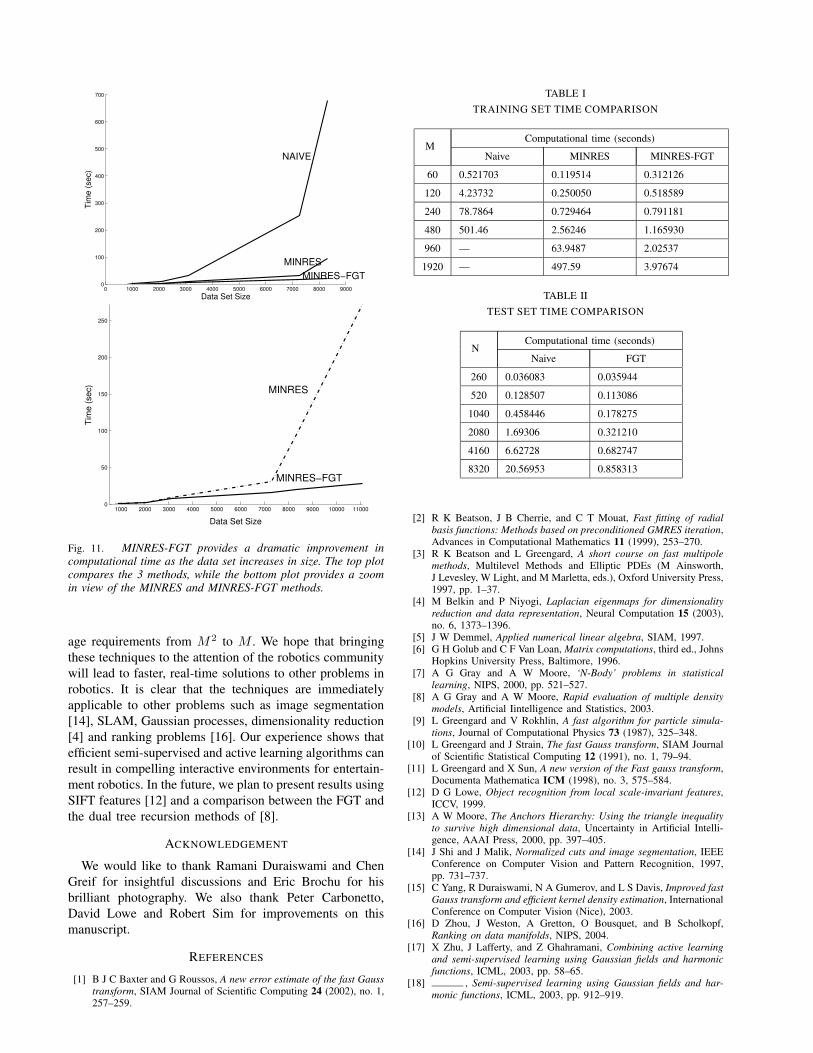
we compared the MINRES-FGT, MINRES, and NAIVEO(M3) algorithms in Matlab using images with differentnumbers of patches. Fig. 11 summarizes the resultingtraining times: both MINRES and MINRES-FGT performdramatically faster even in small data sets with less than50 points. The MINRES-FGT algorithm outperforms MIN-RES in data sets with more than 2000 data points. Althoughthe error given by the error function in Section 2 is lowerin the naive method, MINRES and MINRES-FGT result inless than 0.02 RMS error. Moreover, the difference betweenthe MINRES and MINRES-FGT estimates is less than0.0001.

We also compared the algorithms directly on the Aiboplatform (implemented in C). Table I shows that for areasonably large training set of 960 patches, MINRES-FGT is a factor of 10 times faster than MINRES, whileit becomes computationally prohibitive to run the naivealgorithms for more than 480 patches. Again, we empha-size that MINRES-FGT has a storage requirement of Minstead of M2. Table II shows that the FGT also leadsto significant speed-ups in the kernel discriminant appliedto test set images. For reasonable grid sizes, say 4160 or8320, MINRES-FGT is the only method that can providefast enough solutions for real-time interaction.

VI. CONCLUSION

In this paper, we presented powerful numerical algo-rithms for semi-supervised and active learning that reducethe computational cost from O(M 3) to O(M) and the stor-

0 1000 2000 3000 4000 5000 6000 7000 8000 90000

100

200

300

400

500

600

700

Data Set Size

Tim

e (s

ec)

NAIVE

MINRES MINRES−FGT

1000 2000 3000 4000 5000 6000 7000 8000 9000 10000 110000

50

100

150

200

250

Data Set Size

Tim

e (s

ec) MINRES

MINRES−FGT

Fig. 11. MINRES-FGT provides a dramatic improvement incomputational time as the data set increases in size. The top plotcompares the 3 methods, while the bottom plot provides a zoomin view of the MINRES and MINRES-FGT methods.

age requirements from M2 to M . We hope that bringingthese techniques to the attention of the robotics communitywill lead to faster, real-time solutions to other problems inrobotics. It is clear that the techniques are immediatelyapplicable to other problems such as image segmentation[14], SLAM, Gaussian processes, dimensionality reduction[4] and ranking problems [16]. Our experience shows thatefficient semi-supervised and active learning algorithms canresult in compelling interactive environments for entertain-ment robotics. In the future, we plan to present results usingSIFT features [12] and a comparison between the FGT andthe dual tree recursion methods of [8].

ACKNOWLEDGEMENT

We would like to thank Ramani Duraiswami and ChenGreif for insightful discussions and Eric Brochu for hisbrilliant photography. We also thank Peter Carbonetto,David Lowe and Robert Sim for improvements on thismanuscript.

REFERENCES

[1] B J C Baxter and G Roussos, A new error estimate of the fast Gausstransform, SIAM Journal of Scientific Computing 24 (2002), no. 1,257–259.

TABLE ITRAINING SET TIME COMPARISON

MComputational time (seconds)

Naive MINRES MINRES-FGT

60 0.521703 0.119514 0.312126

120 4.23732 0.250050 0.518589

240 78.7864 0.729464 0.791181

480 501.46 2.56246 1.165930

960 — 63.9487 2.02537

1920 — 497.59 3.97674

TABLE IITEST SET TIME COMPARISON

NComputational time (seconds)

Naive FGT

260 0.036083 0.035944

520 0.128507 0.113086

1040 0.458446 0.178275

2080 1.69306 0.321210

4160 6.62728 0.682747

8320 20.56953 0.858313

[2] R K Beatson, J B Cherrie, and C T Mouat, Fast fitting of radialbasis functions: Methods based on preconditioned GMRES iteration,Advances in Computational Mathematics 11 (1999), 253–270.

[3] R K Beatson and L Greengard, A short course on fast multipolemethods, Multilevel Methods and Elliptic PDEs (M Ainsworth,J Levesley, W Light, and M Marletta, eds.), Oxford University Press,1997, pp. 1–37.

[4] M Belkin and P Niyogi, Laplacian eigenmaps for dimensionalityreduction and data representation, Neural Computation 15 (2003),no. 6, 1373–1396.

[5] J W Demmel, Applied numerical linear algebra, SIAM, 1997.[6] G H Golub and C F Van Loan, Matrix computations, third ed., Johns

Hopkins University Press, Baltimore, 1996.[7] A G Gray and A W Moore, ‘N-Body’ problems in statistical

learning, NIPS, 2000, pp. 521–527.[8] A G Gray and A W Moore, Rapid evaluation of multiple density

models, Artificial Iintelligence and Statistics, 2003.[9] L Greengard and V Rokhlin, A fast algorithm for particle simula-

tions, Journal of Computational Physics 73 (1987), 325–348.[10] L Greengard and J Strain, The fast Gauss transform, SIAM Journal

of Scientific Statistical Computing 12 (1991), no. 1, 79–94.[11] L Greengard and X Sun, A new version of the Fast gauss transform,

Documenta Mathematica ICM (1998), no. 3, 575–584.[12] D G Lowe, Object recognition from local scale-invariant features,

ICCV, 1999.[13] A W Moore, The Anchors Hierarchy: Using the triangle inequality

to survive high dimensional data, Uncertainty in Artificial Intelli-gence, AAAI Press, 2000, pp. 397–405.

[14] J Shi and J Malik, Normalized cuts and image segmentation, IEEEConference on Computer Vision and Pattern Recognition, 1997,pp. 731–737.

[15] C Yang, R Duraiswami, N A Gumerov, and L S Davis, Improved fastGauss transform and efficient kernel density estimation, InternationalConference on Computer Vision (Nice), 2003.

[16] D Zhou, J Weston, A Gretton, O Bousquet, and B Scholkopf,Ranking on data manifolds, NIPS, 2004.

[17] X Zhu, J Lafferty, and Z Ghahramani, Combining active learningand semi-supervised learning using Gaussian fields and harmonicfunctions, ICML, 2003, pp. 58–65.

[18] , Semi-supervised learning using Gaussian fields and har-monic functions, ICML, 2003, pp. 912–919.