fast crc computation for numeric polynomials using ...€¦ · 323102 fast crc computation for...

323102

Fast CRC

Computation for

Generic

Polynomials Using

PCLMULQDQ

Instruction December, 2009

White Paper

Vinodh Gopal

Erdinc Ozturk

Jim Guilford

Gil Wolrich

Wajdi Feghali

Martin Dixon

IA Architects

Intel Corporation

Deniz Karakoyunlu

PhD Student

Worcester Polytechnic Institute

Fast CRC Computation Using PCLMULQDQ Instruction

2


3

Executive Summary This paper presents a fast and efficient method of computing CRC on IA

processors with generic polynomials using the carry-less multiplication

instruction – PCLMULQDQ.

Instead of reducing the entire message with traditional reduction

algorithms, we use a faster folding approach to reduce an arbitrary length

buffer to a small fixed size to be reduced further by traditional methods

such as Barrett reduction.

Parallelized folding approach is used to maximize the throughput of

PCLMULQDQ instructions. We show how to do this efficiently for data

buffers of arbitrary length.

The final reduction part is only slightly different for different sized

polynomials (e.g., a 32-bit CRC and a 16-bit CRC).

With our novel folding methods, CRC computation using PCLMULQDQ

is faster than best software routines that don’t use the instruction, on

a range of IA processor cores.

This paper will enable customers to code and optimize any CRC

application for maximum performance on Westmere. We use real

examples in the paper to illustrate the methods.


4

Contents

Background ............................................................................................................. 5

Overview of CRC computation ................................................................................... 5

PCLMULQDQ Instruction ......................................................................... 7

Fast CRC Computation .............................................................................................. 7

Overview of the Folding Method .............................................................. 7 Single fold of a 128-bit Data chunk .............................................. 10 Parallel Folding of 128-bit Data chunks ........................................ 11

Detailed Implementation Steps for 32-bit CRC ........................................ 11 Step 1 – Iteratively Fold by 4: .................................................... 11 Step 2 – Iteratively Fold by 1: .................................................... 12 Step 3 - Final Reduction of 128-bits ............................................. 13 Overall flow ............................................................................... 14 Example of 32-bit CRC (IEEE 802.3) ............................................ 16

16-bit CRC ............................................................................................................ 16

64-bit CRC ............................................................................................................ 17

Final Reduction of 128-bits ......................................................... 17

Bit-Reflection ........................................................................................................ 18

Example of 32-bit CRC with bit-reflected data (gzip CRC) ............... 21

Conclusion ............................................................................................................ 22

323102

Background

A Cyclic Redundancy Check (CRC) is the remainder, or residue, of binary division of a potentially long message, by a CRC polynomial. This technique

is ubiquitously employed in communication and storage applications due to its effectiveness at detecting errors and malicious tampering. It is a simple operation; one merely applies the CRC to calculate the residue of the data one wishes to protect and appends it to the end of the data stream. When the transmission is received or the stored data is retrieved, the CRC residue is re-generated and confirmed against the appended residue.

With the explosion of high-speed networking and the dramatic increase in storage demands over the past decade, CRC residue generation has become a significantly harder problem. Data networks transmitting 10 Gigabits/second of data are commonplace, with even faster networks on the horizon. Designers in the networking and storage space are challenged to support many different CRC polynomials due to the multiplicity of

mainstream transmission protocols. Due to the conflicting demands of increased speed and polynomial flexibility, it is highly desirable to have a system that can satisfy both of these requirements simultaneously.

Overview of CRC computation

We can define the CRC value of a message M of any length, corresponding to the binary polynomial M (x) as:

CRC (M (x)) = xdeg(P(x)) • M(x) mod P (x)

where the polynomial P(x) defines the CRC algorithm and the symbol “•” denotes carry-less multiplication.

For a 32 bit CRC algorithm, P(x) is a polynomial of degree 32.


6

Figure 1. 32-bit CRC Operation

Arbitrary length Data

CRC Value

CRC

32

CRC can be computed as the modular residue of a large polynomial defined over the Galois field GF(2) with respect to the CRC polynomial. An example illustrating this fact for a 32-bit CRC is shown in Figure 1. Modular reduction

over binary fields can be performed efficiently using Barrett/Montgomery style reductions if we can perform efficient carry-less multiplication. If there is no efficient carry-less multiplication, the traditional methods use multiple lookup tables to compute the CRC – these methods are not as fast as our methods using carry-less multiplication and suffer from the need to store large lookup tables per polynomial.

In the following discussions, we focus on 32-bit CRC to illustrate the main points; however, these points apply to polynomials of other sizes as well. A straightforward implementation of 32-bit CRC operation using carry-less multiplication, requires reducing 64 bits of data down to 32-bits at each iteration using the traditional GF(2) reduction methods. This reduction is

expensive, because it needs two dependent carry-less multiplication operations for each iteration and reduces 32 bits of the data. Alternatively, the data can be repeatedly folded down by 128 bits at a time, taking advantage of the PCLMULQDQ carry-less multiplication instruction. Using this approach, the reduction to 32-bits will be necessary only at the end yielding a faster reduction scheme.


7

PCLMULQDQ Instruction

PCLMULQDQ instruction performs carry-less multiplication of two 64-bit quadwords which are selected from the first and the second operands according to the immediate byte value.

Instruction format: PCLMULQDQ xmm1, xmm2/m128, imm8 Description: Carry-less multiplication of one quadword (8-byte) of xmm1 by one quadword (8-byte) of xmm2/m128, returning double quadwords (16 bytes). The immediate byte is used for determining which quadwords of xmm1 and xmm2/m128 should be used. Due to the nature of carry-less

multiplication, the most-significant bit of the result will be 0. Opcode: 66 0f 3a 44 The presence of PCLMULQDQ is indicated by the CPUID leaf 1 ECX[1]. Operating systems that support the handling of Intel SSE state will also support applications that use AES extensions and the PCLMULQDQ

instruction. This is the same requirement for Intel SSE2, Intel SSE3, Intel SSSE3, and Intel SSE4.

The immediate byte values are used as follows:

imm[7:0] Operation

0x00 xmm2/m128[63:0] • xmm1[63:0]

0x01 xmm2/m128[63:0] • xmm1[127:64]

0x10 xmm2/m128[127:64] • xmm1[63:0]

0x11 xmm2/m128[127:64] • xmm1[127:64]

Fast CRC Computation

Overview of the Folding Method

For any application that requires CRC one can pre-compute a few constants (that are a function of the polynomial) and then repeatedly apply these constants to fold the most-significant chunks of the data buffer, at each

stage creating a new buffer that is smaller in length but congruent (modulo the polynomial) to the original one, as illustrated in Figure 2.


8

Figure 2. General Description of Folding a Data Buffer

XORsMultiplicationsConstants

In Figure 2, we show folding in its simplest form, where a most-significant

chunk of data is folded into an adjacent chunk of the same size reducing the data buffer to one that is smaller in length by the length of the chunk.

In Figure 3, we show a more generalized approach to folding where we fold the most-significant chunk to an arbitrary position in the data buffer. More specifically, let D(x) and G(x) be the most significant 128-bit and remaining

T-bit (T >= 128) chunks respectively of a data buffer M(x). In order to fold 128 bits of data, we could compute D(x) • [xT mod P(x)] and XOR (bit-wise exclusive or) it with G(x). This follows from the fact that:

M(x) = D(x) • xT G(x)

M(x) mod P(x) {D(x) • [xT mod P(x)] G(x)} mod P(x)

We can precompute [xT mod P(x)], which would be a 32-bit constant for 32-bit CRC. The product D(x) • [xT mod P(x)] would yield a (128+32) 160-bit result which cannot be handled efficiently in a typical SSE2 architecture.

Therefore, we treat D(x) as two 64-bit chunks: H(x) and L(x). Then the following computation will result in a reduced 96-bit data chunk that is congruent to D(x) • xT modulo P(x):

D(x) • [xT mod P(x)] {H(x) • [x(T+64) mod P(x)]} {L(x) • [xT mod

P(x)]}


9

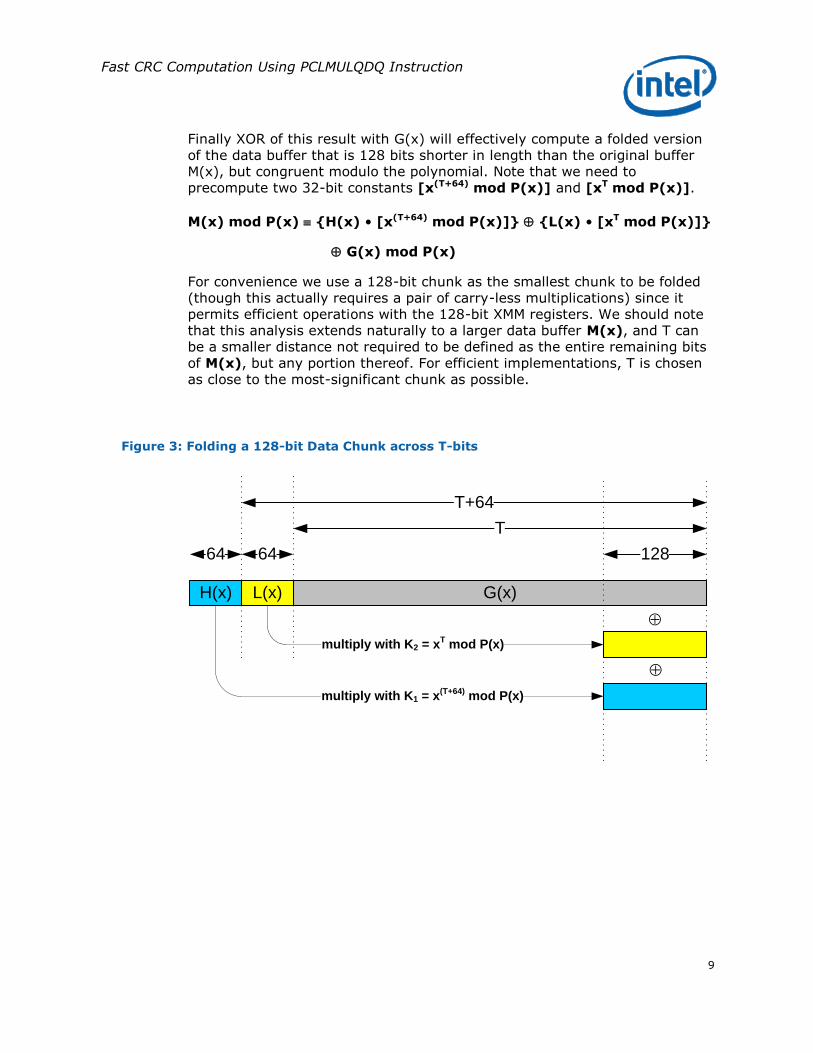
Finally XOR of this result with G(x) will effectively compute a folded version

of the data buffer that is 128 bits shorter in length than the original buffer M(x), but congruent modulo the polynomial. Note that we need to precompute two 32-bit constants [x(T+64) mod P(x)] and [xT mod P(x)].

M(x) mod P(x) {H(x) • [x(T+64) mod P(x)]} {L(x) • [xT mod P(x)]}

G(x) mod P(x)

For convenience we use a 128-bit chunk as the smallest chunk to be folded (though this actually requires a pair of carry-less multiplications) since it permits efficient operations with the 128-bit XMM registers. We should note that this analysis extends naturally to a larger data buffer M(x), and T can be a smaller distance not required to be defined as the entire remaining bits

of M(x), but any portion thereof. For efficient implementations, T is chosen as close to the most-significant chunk as possible.

Figure 3: Folding a 128-bit Data Chunk across T-bits

G(x)L(x)H(x)

T

T+64

128

multiply with K1 = x(T+64)

mod P(x)

multiply with K2 = xT mod P(x)

64 64


10

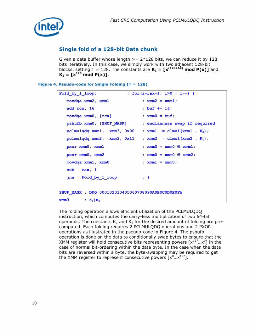
Single fold of a 128-bit Data chunk

Given a data buffer whose length >= 2*128 bits, we can reduce it by 128 bits iteratively. In this case, we simply work with two adjacent 128-bit blocks, setting T = 128. The constants are K1 = [x(128+64) mod P(x)] and K2 = [x128 mod P(x)].

Figure 4. Pseudo-code for Single Folding (T = 128)

Fold_by_1_loop: ; for(i=rax-1; i>0 ; i--) {

movdqa xmm2, xmm1 ; xmm2 = xmm1;

add rcx, 16 ; buf += 16;

movdqa xmm0, [rcx] ; xmm0 = buf;

pshufb xmm0, [SHUF_MASK] ; endianness swap if required

pclmulqdq xmm1, xmm3, 0x00 ; xmm1 = clmul(xmm1 , K2);

pclmulqdq xmm2, xmm3, 0x11 ; xmm2 = clmul(xmm2 , K1);

pxor xmm0, xmm1 ; xmm0 = xmm0 xmm1;

pxor xmm0, xmm2 ; xmm0 = xmm0 xmm2;

movdqa xmm1, xmm0 ; xmm1 = xmm0;

sub rax, 1

jne Fold_by_1_loop ; }

SHUF_MASK : DDQ 000102030405060708090A0B0C0D0E0Fh

xmm3 : K1|K2

The folding operation allows efficient utilization of the PCLMULQDQ instruction, which computes the carry-less multiplication of two 64-bit operands. The constants K1 and K2 for the desired amount of folding are pre-computed. Each folding requires 2 PCLMULQDQ operations and 2 PXOR operations as illustrated in the pseudo-code in Figure 4. The pshufb operation is done on the data to conditionally swap bytes to ensure that the

XMM register will hold consecutive bits representing powers [x127…x0] in the case of normal bit-ordering within the data byte. In the case when the data bits are reversed within a byte, the byte-swapping may be required to get the XMM register to represent consecutive powers [x0…x127].


11

Parallel Folding of 128-bit Data chunks

In order to further maximize the efficiency of folding, it can be applied on different chunks of the data in a parallel manner as shown in Figure 5.

Figure 5: Folding 4 128-bit Data Chunks in parallel

X3 X2 X1 X0

XOR

XOR

XOR

XOR

fold fold fold fold

Thus for buffers that are suitably large (length >= 2*(4*128) bits), we can iteratively reduce by 4 folding operations for maximal efficiency, until we have a congruent buffer that is much smaller.

Each of the 4 folds is identical – we work on 128-bit data chunks using the constants K1 = [x(512+64) mod P(x)] and K2 = [x512 mod P(x)]. This

corresponds to T = 4*128 = 512.

Detailed Implementation Steps for 32-bit CRC

In this section, we describe the steps required to reduce an arbitrary data buffer to the final CRC, using parallel, single folds and traditional reduction methods to generate the final CRC. For ease of illustration, we assume the data buffer is large enough that it will require all the steps in this section and we assume a 32-bit CRC. We denote the constants in the various steps as ki.

Step 1 – Iteratively Fold by 4:

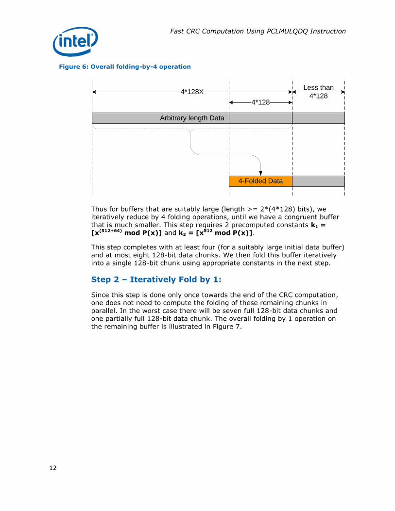
The parallel folding by 4 operations on an arbitrary length buffer is illustrated in Figure 6.


12

Figure 6: Overall folding-by-4 operation

Arbitrary length Data

4-Folded Data

4*128

4*128XLess than

4*128

Thus for buffers that are suitably large (length >= 2*(4*128) bits), we iteratively reduce by 4 folding operations, until we have a congruent buffer

that is much smaller. This step requires 2 precomputed constants k1 = [x(512+64) mod P(x)] and k2 = [x512 mod P(x)].

This step completes with at least four (for a suitably large initial data buffer) and at most eight 128-bit data chunks. We then fold this buffer iteratively into a single 128-bit chunk using appropriate constants in the next step.

Step 2 – Iteratively Fold by 1:

Since this step is done only once towards the end of the CRC computation, one does not need to compute the folding of these remaining chunks in parallel. In the worst case there will be seven full 128-bit data chunks and

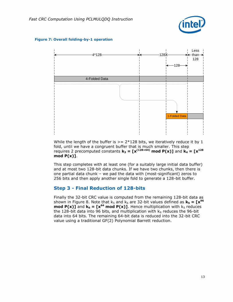
one partially full 128-bit data chunk. The overall folding by 1 operation on the remaining buffer is illustrated in Figure 7.


13

Figure 7: Overall folding-by-1 operation

4-Folded Data

1-Folded Data

4*128

Less

than

128

128X

128

While the length of the buffer is >= 2*128 bits, we iteratively reduce it by 1 fold, until we have a congruent buffer that is much smaller. This step requires 2 precomputed constants k3 = [x(128+64) mod P(x)] and k4 = [x128 mod P(x)].

This step completes with at least one (for a suitably large initial data buffer) and at most two 128-bit data chunks. If we have two chunks, then there is one partial data chunk – we pad the data with (most-significant) zeros to 256 bits and then apply another single fold to generate a 128-bit buffer.

Step 3 - Final Reduction of 128-bits

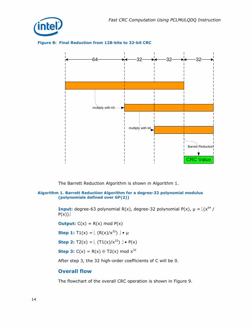
Finally the 32-bit CRC value is computed from the remaining 128-bit data as shown in Figure 8. Note that k5 and k6 are 32-bit values defined as k5 = [x96 mod P(x)] and k6 = [x64 mod P(x)]. Hence multiplication with k5 reduces the 128-bit data into 96 bits, and multiplication with k6 reduces the 96-bit data into 64 bits. The remaining 64-bit data is reduced into the 32-bit CRC

value using a traditional GF(2) Polynomial Barrett reduction.


14

Figure 8: Final Reduction from 128-bits to 32-bit CRC

32

CRC Value

64 32

multiply with k5

multiply with k6

Barrett Reduction

32

The Barrett Reduction Algorithm is shown in Algorithm 1.

Algorithm 1. Barrett Reduction Algorithm for a degree-32 polynomial modulus (polynomials defined over GF(2))

Input: degree-63 polynomial R(x), degree-32 polynomial P(x), µ = (x64 /

P(x))

Output: C(x) = R(x) mod P(x)

Step 1: T1(x) = (R(x)/x32) • µ

Step 2: T2(x) = (T1(x)/x32) • P(x)

Step 3: C(x) = R(x) T2(x) mod x32

After step 3, the 32 high-order coefficients of C will be 0.

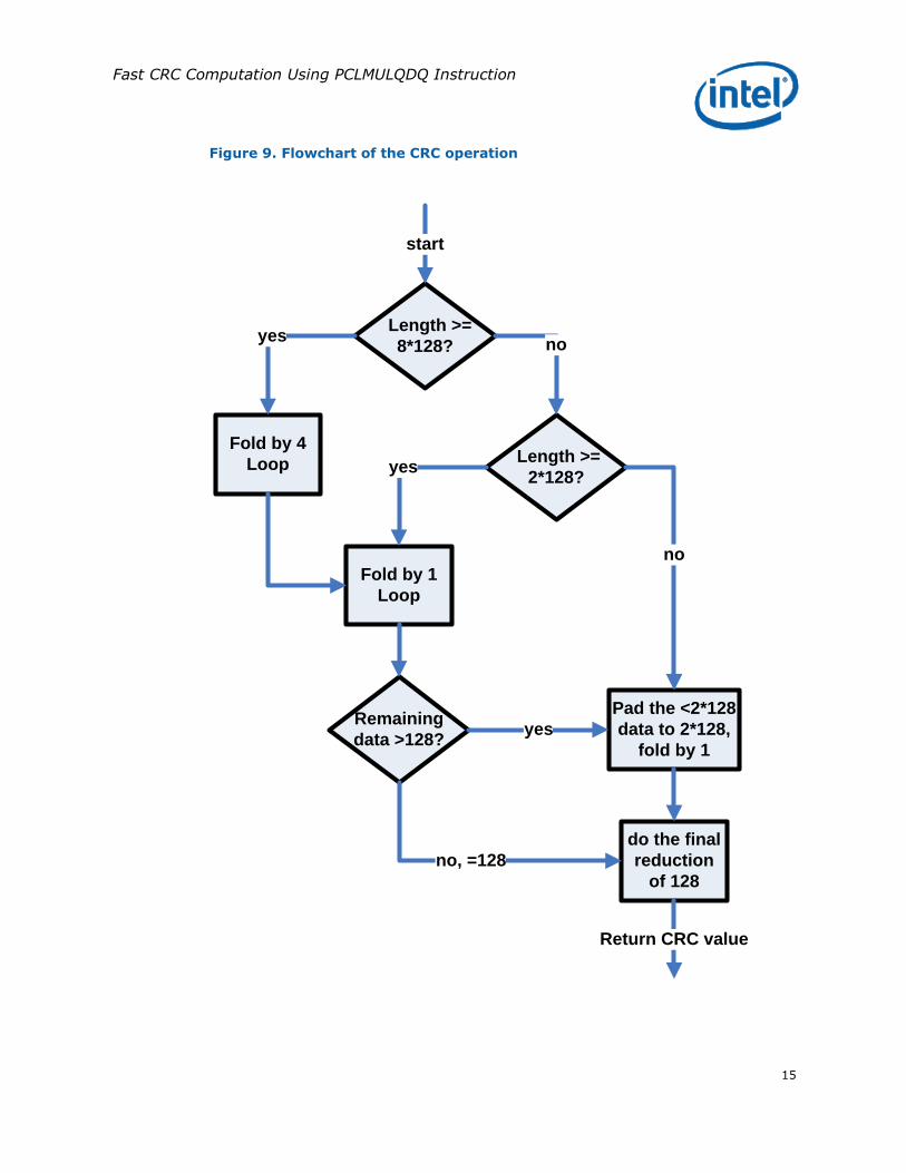
Overall flow

The flowchart of the overall CRC operation is shown in Figure 9.


15

Figure 9. Flowchart of the CRC operation

Fold by 4

Loop

Length >=

8*128?

Fold by 1

Loop

Length >=

2*128?

Pad the <2*128

data to 2*128,

fold by 1

do the final

reduction

of 128

yesno

yes

no

Return CRC value

Remaining

data >128?yes

no, =128

start


16

Example of 32-bit CRC (IEEE 802.3)

These methods can be applied as an example to the IEEE 802.3 CRC. These are the key constants that need to be computed for this example. For other 32-bit CRC applications, the constants need to be recomputed using the formulae given in the previous sections.

• P(x) = 0x104C11DB7;

• k1 = x4*128+64 mod P(x) = 0x8833794C

• k2 = x4*128 mod P(x) = 0xE6228B11

• k3 = x128+64 mod P(x) = 0xC5B9CD4C

• k4 = x128 mod P(x) = 0xE8A45605

• k5 = x96 mod P(x) = 0xF200AA66

• k6 = x64 mod P(x) = 0x490D678D

• = x64/P(x) = 0x104D101DF

16-bit CRC

If the CRC is required for a polynomial of degree smaller than 32, say 16, the same methods described above, will work if we use a modulus scaling approach. We use the property:

A B mod C A•K B•K mod C•K

This means that, if we multiply the modulus (C) and the number to be reduced (A) with the same constant, then the intermediate result of the modular operation using these modified values will be (B•K) – this intermediate result can be divided with the same constant to achieve B, which is the desired result.

If our polynomial P(x) is of degree 16, we multiply it with x16 and achieve a 32-degree polynomial Q(x). In a 32-bit CRC operation, the data buffer to be reduced is multiplied with x32. For the 16-bit CRC, instead of multiplying the data buffer with x16, we multiply it with x32 to achieve the same scaling as modulus polynomial. Now that both modulus and operand are scaled with

the same constant, x16, we can proceed with the 32-bit CRC algorithm described above. The constants are also pre-computed using the scaled modulus polynomial Q(x). At the very end of the CRC operation, the most significant 16 bits of the final CRC value are returned (the lower 16 bits are zero).


17

For 16-bit CRC we should note that the suggested method is also optimal in

addition to being convenient - we cannot take advantage of the smaller size of the CRC polynomial and find a faster implementation since the carry-less multiplication instruction is defined on a fixed operand size of 64 bits.

64-bit CRC

If we have applications that require a CRC with a polynomial degree greater than 32, we can use similar techniques described in the previous sections to compute a 64 bit CRC.

The process of folding is exactly the same (with different constants) with minor differences in the final reduction flow.

Final Reduction of 128-bits

In the 3rd Step, the 64-bit CRC value is computed from the remaining 128-bit data as shown in Figure 10. Note that k5 is a 64-bit value defined as k5 = [x128 mod P(x)]. The remaining 128-bit data is reduced into the 64-bit CRC value using a traditional GF(2) Polynomial Barrett reduction

Figure 10. Final reduction from 128 bits to 64-bit CRC

32

CRC Value

64 32

multiply with k5

Barrett Reduction

64


18

The Barrett Reduction Algorithm is shown in Algorithm 2.

Algorithm 2. Barrett Reduction Algorithm for a degree-64 polynomial modulus (polynomials defined over GF(2))

Input: degree-127 polynomial R(x), degree-64 polynomial P(x), µ = (x128 /

P(x))

Output: C(x) = R(x) mod P(x)

Step 1: T1(x) = (R(x)/x64) • µ

Step 2: T2(x) = (T1(x)/x64) • P(x)

Step 3: C(x) = R(x) T2(x) mod x64

After step 3, the 64 high-order coefficients of C will be 0.

Note that since P(x) and µ are 65 bits in length, the carry-less multiplication has to be performed with a PCLMULQDQ and an XOR operation.

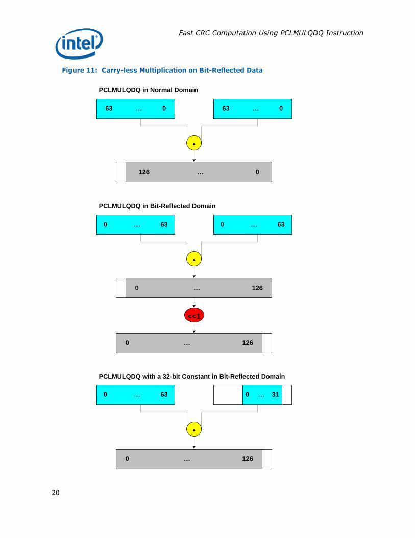
Bit-Reflection

Some CRC applications work on bit-reflected data. In such cases, our methodology can be efficiently applied in a bit-reflected domain without a

need for back and forth bit reflections. This is possible, because PCLMULQDQ and PXOR operations are bit-order agnostic. However, the 127-bit result of carry-less multiplication of two 64-bit numbers is stored into the least significant 127-bits of the 128-bit XMM register. In the bit-reflected domain, a left-shift is needed after a carry-less multiplication in order to preserve the correct result. This can be described by the following property of carry-less

multiplication of bit-reflected operations:

(bit-reflected(A) •bit-reflected(B)) << 1 = bit-reflected(A•B)

where the bit-reflection on A and B is performed on their size (n bits) and the bit-reflection on the product is performed over 2n bits.

One possible optimization is to do the left-shift on one of the multiplicands prior to the multiplication of bit-reflected operands. In the folding methods described above for 32-bit CRC, multiplications take place between the data and a pre-computed (32-bit) constant. If this constant is generated in already left-shifted form, carry-less multiplication of bit-reflected operands will compute the correct result without a need for a following left-shift on

the result. With this optimization, the reflected constant will be 33 bits in length as shown in Figure 11. Note that we need to compute the folding constants differently, such that when we perform a bit-reflection, the constants occupy least-significant-bit (lsb) positions (to permit us to perform a left-shift operation). The example for bit-reflected application shown in the


19

next sub-section illustrates this (contrast it with the previous example for

normal bit ordering of IEEE 802.3).

Another way to accomplish the same efficiency during folding is to compute the constants differently and keep the size of the reflected constant the same i.e., 32 bits. Consider the example of k4 = x128 mod P(x); to generate the equivalent constant for reflected operations, we could instead

generate k4 = x128-1 mod P(x), in bit-reflected form – the PCLMULQDQ operation in bit-reflected domain scales the product by x, compensating for the “-1” in the exponent of the new constant. Thus no shifting of the product will be needed. In either method, we can reuse the same code (with different constants). For the rest of the discussion however, we focus on the first method.


20

Figure 11: Carry-less Multiplication on Bit-Reflected Data

63 … 0 63 … 0

•

126 … 0

0 … 63 0 … 63

•

0 … 126

<<1

0 … 126

PCLMULQDQ in Normal Domain

PCLMULQDQ in Bit-Reflected Domain

0 … 63 0 … 31

•

PCLMULQDQ with a 32-bit Constant in Bit-Reflected Domain

0 … 126


21

The final Barrett reduction of the CRC for the bit-reflected input has the

same steps as the normal version. The only difference will be the alignment of the data and the requirement to select data from different parts of the intermediate results. Figure 12 illustrates the Barrett steps for normal and bit-reflected inputs and shows the difference. The notation X’ denotes a bit-reflected form of X – formally defined as X’[i] = X[n-1-i] for i=0 through (n-1), where X has n bits and [i] refers to the ith least-significant bit of X.

Figure 12. Polynomial (GF(2)) Barrett Reduction steps for normal and bit-reflected input

0

R(x)

Xmm register

µ

33

•

0

32

P(x)

33

•Step 2: T2(x) = (T1(x)/x32

)• P(x)

Step 1: T1(x) = (R(x)/x32

)•µ

0 T2(x)

T1(x)

T2(x)

0

R(x)’

Xmm register

µ’

33

•

0

32

P(x)’

33

•

0 T2(x)' T2(x)'

T1(x)'

Step 1: T1(x)' = (R(x)’ mod x32

)•µ’

Step 2: T2(x)' = (T1(x)' mod x32

)• P(x)’

Example of 32-bit CRC with bit-reflected data (gzip CRC)

The above methods can be applied as an example to the gzip CRC that

operates on bit-reflected data. These are the constants that need to be computed for this example. Note that the constants need to be computed using the formulae given in this example. P(x)’ and µ’ are 33-bit reflected constants, whereas other constants are 64-bit reflections.


22

Bit-reflected constants:

• P(x)’ = 0x1DB710641;

• k1’ = (x4*128+32 mod P(x) << 32)’ << 1 = 0x154442bd4

• k2’ = (x4*128-32 mod P(x) << 32)’ << 1 = 0x1c6e41596

• k3’ = (x128+32 mod P(x) << 32)’ << 1 = 0x1751997d0

• k4’ = (x128-32 mod P(x) << 32)’ << 1 = 0x0ccaa009e

• k5’ = (x64 mod P(x) << 32)’ << 1 = 0x163cd6124

• k6’ = (x32 mod P(x) << 32)’ << 1 = 0x1db710640

• ’ = (x64/P(x))’ = 0x1F7011641

§

Conclusion

We presented a fast and efficient method of computing CRC on IA processors with generic polynomials using the carry-less multiplication

instruction – PCLMULQDQ. This instruction has been introduced in the Westmere processor.

Instead of reducing the entire message with traditional reduction algorithms, we use a faster folding approach to reduce an arbitrary length buffer to a small fixed size to be reduced further by traditional methods such as Barrett

reduction over GF(2) polynomials.

A Parallelized folding approach is used to maximize the throughput of PCLMULQDQ instructions. We show how to do this efficiently for data buffers of arbitrary length. This method enables good performance on a range of IA cores that will support the PCLMULQDQ instruction.

Using PCLMULQDQ, we can compute CRC for any polynomial without the need for large lookup-tables as required by conventional software methods. The methods for computing CRC described in this paper will also permit much faster computations than the best lookup-table based software approaches.


23

The Intel® Embedded Design Center provides qualified developers with web-based access to technical resources. Access Intel Confidential design materials, step-by step guidance, application reference solutions, training, Intel’s tool loaner program, and connect with an e-help desk and the embedded community. Design Fast. Design Smart. Get started today. http://intel.com/embedded/edc.

Authors

Vinodh Gopal, Erdinc Ozturk, Jim Guilford, Gil Wolrich, Wajdi Feghali and Martin Dixon are are IA Architects with the IAG

Group at Intel Corporation.

Deniz Karakoyunlu is a PhD student at the Worcester Polytechnic Institute.

INFORMATION IN THIS DOCUMENT IS PROVIDED IN CONNECTION WITH INTEL® PRODUCTS. NO LICENSE, EXPRESS OR IMPLIED, BY ESTOPPEL OR OTHERWISE, TO ANY INTELLECTUAL PROPERTY RIGHTS IS GRANTED BY THIS DOCUMENT. EXCEPT AS PROVIDED IN INTEL’S TERMS AND CONDITIONS OF SALE FOR SUCH PRODUCTS, INTEL ASSUMES NO LIABILITY WHATSOEVER, AND INTEL DISCLAIMS ANY EXPRESS OR IMPLIED WARRANTY, RELATING TO SALE AND/OR USE OF INTEL PRODUCTS INCLUDING LIABILITY OR WARRANTIES RELATING TO FITNESS FOR A PARTICULAR PURPOSE, MERCHANTABILITY, OR INFRINGEMENT OF ANY PATENT, COPYRIGHT OR OTHER INTELLECTUAL PROPERTY RIGHT. Intel products are not intended for use in medical, life saving, or life sustaining applications.

Intel may make changes to specifications and product descriptions at any time, without notice.

This paper is for informational purposes only. THIS DOCUMENT IS PROVIDED "AS IS" WITH NO

WARRANTIES WHATSOEVER, INCLUDING ANY WARRANTY OF MERCHANTABILITY,

NONINFRINGEMENT, FITNESS FOR ANY PARTICULAR PURPOSE, OR ANY WARRANTY OTHERWISE

ARISING OUT OF ANY PROPOSAL, SPECIFICATION OR SAMPLE. Intel disclaims all liability, including

liability for infringement of any proprietary rights, relating to use of information in this specification.

No license, express or implied, by estoppel or otherwise, to any intellectual property rights is granted

herein.

BunnyPeople, Celeron, Celeron Inside, Centrino, Centrino logo, Core Inside, Dialogic, FlashFile, i960,

InstantIP, Intel, Intel logo, Intel386, Intel486, Intel740, IntelDX2, IntelDX4, IntelSX2, Intel Core, Intel

Inside, Intel Inside logo, Intel. Leap ahead., Intel. Leap ahead. logo, Intel NetBurst, Intel NetMerge,

Intel NetStructure, Intel SingleDriver, Intel SpeedStep, Intel EP80579 Integrated Processor, Intel

StrataFlash, Intel Viiv, Intel vPro, Intel XScale, IPLink, Itanium, Itanium Inside, MCS, MMX, Oplus,

OverDrive, PDCharm, Pentium, Pentium Inside, skoool, Sound Mark, The Journey Inside, VTune,

Xeon, and Xeon Inside are trademarks or registered trademarks of Intel Corporation or its

subsidiaries in the U.S. and other countries.

*Other names and brands may be claimed as the property of others.

Copyright © 2009 Intel Corporation. All rights reserved.

http://intel.com/embedded/edc

fast crc computation for numeric polynomials using ...€¦ · 323102 fast crc computation for...

Documents