fast detection and display of symmetry in outerplanar graphs

Discrete Applied Mathematics 39 (1992) 13-35

North-Holland 13

Fast detection and display of symmetry in outerplanar graphs

Joseph Manning* and Mikhail J. Atallah Department of Computer Sciences, Purdue University, West Lafayette, IN 47907, USA

Received 27 January 1989

Revised 2 April 1990

Abstract

Manning, J. and M. J. Atallah, Fast detection and display of symmetry in outerplanar graphs,

Discrete Applied Mathematics 39 (1992) 13-35.

The automatic construction of good drawings of abstract graphs is a problem of practical impor-

tance. Symmetry appears as one of the main criteria for achieving goodness. Algorithms are

developed for enumerating all planar axial and rotational symmetries of a biconnected outer-

planar graph, and it is shown how to construct a drawing which simultaneously displays all these

symmetries. These results are then expanded to obtain algorithms for the detection and display

of outerplanar axial and rotational symmetry in the entire class of outerplanar graphs. All

algorithms run in both time and space which are linear in the size of the graph, and hence are

optimal to within a constant factor.

1. Drawing graphs

Mathematically, an abstract graph simply consists of two sets, V and E c V/x V,

and as such is completely specified by an enumeration of these sets or by adjacency lists or an adjacency matrix [ 11. However, such representations convey little structural information about the graph, and so graphs are instead often presented by means of drawings. Every given abstract graph may be drawn in various different ways, all equally “correct”, but some certainly “better” than others in the sense that they clearly display important structural properties of the graph. For example, both drawings in Fig. 1 represent the same abstract graph (the Herschel graph), but key properties such as planarity, biconnectivity, symmetry, diameter, and even bi- partition are readily apparent from the second drawing but not from the first.

As discussed in [12], there are many different and -ometimes conflicting criteria which may be used to guide the construction of good drawings of a graph. Amongst

* Current address: Department of Computer Science, Vassar College, Poughkeepsie, NY 12601, USA.

0166-218X/92/$05.00 0 1992-Elsevier Science Publishers B.V. All rights reserved

J. Manning, M.J. Atallah

Fig. 1. Tv;o drawings of the same graph.

these, the best overall general criteria appear to be the display of axial symmetry and, to a somewhat lesser extent, the display of rotational symmetry. It should be emphasized here that both axial and rotational symmetry are inherent properties of the abstract graph, independent of any particular drawing. In fact these properties can be formally defined in a purely algebraic manner in terms of automorphisms of the graph. However, for the present study it is more convenient to work with the equivalent geometric concept: an abstract t raph is defined to have an axial (rotational) symmetry if there is some drawing of the graph which displays that axial (rotational) symmetry in the geometric sense.

Here, a (straight-edge) drawing of a graph consists of a set of distinct disks in the plane, one disk for each vertex, with straight-line segments between disks representing adjacent vertices. To avoid ambiguous representations, a line segment may not intersect a disk unless the corresponding edge and vertex are incident. Note that for simplicity, all drawings considered here use straight-line segments to draw edges; this restriction ensures that a drawing of a graph is fully specified merely by the positions of its vertices, and also does not conflict with the display of either symmetry or planarity [7].

Despite their significance in the construction of visually informative drawings, the basic problems of detecting any axial or rotational symmetry in general graphs appear to be computationally intractable, with the associated counting problems being correspondingly difficult, as shown by the following results:

Theorem 1.1 [ 1 I]. The problems of determining if an abitrary graph has any axial symmetry or any rotational symmetry are both NP-complete.

Theorem 1.2 [I l]. The problems of counting the number of axial symmetries or rotational symmetries in an arbitrary graph are both #P-complete.

Planar graphs constitute an important subclass of general graphs, and frequently admit efficient solutions to problems which are generally NP-complete. Moreover,

Symmetry in outerplanar graphs 15

the graphs used in the proofs of the above theorems are nonplanar, so the present research has accordingly focussed on symmetry in planar graphs. Linear algorkhms

have already been obtained in [12] for detection, enumeration, and display of axial and rotational symmetry in trees; this paper now extends those results by establishing corresponding algorithms for outerplanar graphs.

A planar symmetry of a graph is a symmetry which can be displayed in a planar drawing of the graph. Clearly, only planar graphs can have planar symmetries, although they may also have nonplanar symmetries.

Since planarity is a desirable general property in drawings of outerplanar graphs, only planar drawings, and so only planar symmetries, are considered in this paper. In addition, only undirected simple graphs are considered; however, all the results have natural extensions to directed graphs and to graphs with loops and parallel edges. The adjacency list representation of graphs is assumed in all the algorithms. For the basic definitions and concepts of graph theory not explicitly presented here, consult any standard text such as [3,4,8].

2. Outerplanar graphs and biconnectivity

The existing definitions, theorems and algorithms concerning those aspects of outerplanarity and biconnectivity relevant to the problem of symmetry detection are collected together and stated below:

Definition. A graph is outer-planar if it has a planar embedding in which every vertex lies on the outer face.

Algorithm 2.1 [ 131. An O(n)-time algorithm to test if an n-vertex graph is outerplanar.

Definition. A cutvertex of a connected graph is any vertex whose removal would disconnect the graph. A graph is biconnected if it is connected and has no cutvertex. The Blocks of a graph are its maximal biconnected subgraphs. (Cutvertices and blocks are also called articulation points and biconnected components, respectively.)

The blocks of a connected graph form a special tree-like structure:

Definition. The block-cutvertex tree of a connected graph is the tree which has a vertex for every block and every cutvertex of the graph, and an edge between the image of every cutvertex and the images of all blocks containing it.

This block-cutvertex tree can be constructed efficiently by using:

Algorithm 2.2 [I]. An O(m)-time algorithm to decompose a connected cyz edges into its blocks.

graph with

16 J. Manning, M.J. Atallah

An important link between outerplanarity and biconnectivity is established by the following theorem:

Theorem 2.3 [g]. A graph is outerplanar iff each of its blocks is outerplanar.

The significance of biconnectivity to the development of symmetry algorithms for outerplanar graphs stems from:

Theorem 2.4 [6]. Ever-v biconnected outerplanar graph with at least three vertices has a unique Hamilton cycle.

Furthermore, this Hamilton cycle can be obtained efficiently from:

Algorithm 2.5 [13]. An O(n)-time algorithm to find the Hamilton cycle of a bicon- netted outerplanar graph with n ~3 vertices.

3. Detecting symmetry in biconnected outerplanar graphs

Let G be any biconnected outerplanar graph. The essence of the following symmetry detection algorithms is to encode G into a string S, in such a way that planar symmetries of G correspond to certain string symmetries of S. Efficient pattern- matching techniques are then used to enumerate these string symmetries, from which the original graph symmetries are easily recovered. (This method was applied in [2,9,15] to detect symmetries of geometric figures; the present application, by contrast, occurs in a purely combinatorial setting.)

Let G have n vertices and m edges; assume nz 3, since symmetry detection is trivial for n < 3, and recall that outerplanarity implies m s 2n - 3. The actual encoding of G resembles that used in [6] for an outerplanar isomorphism test. Using Algorithm 2.5, the unique Hamilton cycle H of G is first obtained, and one of its two possible orientations is arbitrarily assigned to H. For each vertex v, each incident edge (v, w) is encoded as an ordered pair of integers, denoting the distances from v to w along M in the chosen orientation and reverse orientation, respectively. Vertex v is then encoded by the string c(v) consisting of the concatenation of these ordered pairs, sorted in ascending order by first component. Figure 2 shows a graph, and the encoding of vertices based on a clockwise orientation of its Hamilton cycle.

A string S which encodes G is then constructed by starting from any vertex and traversing H along the chosen orientation, concatenating the encodings of the vertices as they are encountered. Since S depends on the selected starting vertex, it is subscripted with the name of that vertex. For example, in Fig. 2,

SA=15245115511542511524511551154251.

Let v - i and v + i, for Or is n - 1, denote respectively the ith predecessor and ith successor of vertex v along Hin the chosen orientation. Let + (s, k) denote the result


154251 152451

152451 154251

Fig. 2. Encoding of vertices, under clockwise orientation of the Hamilton cycle.

of removing the leftmost k elements of any string s and appending them, in order, to the right end of s; this operation is known as a Ief cyclic shift.

The following properties then hold for the string S,,, for each vertex u: l Although the n possible choices for u generate n corresponding encodings SU,

these strings differ from one another only by cyclic shifts; for any 0~ is n - 1,

l The structure of G can be fully recovered from S,, regardless of the choice of u or the orientation of H. In decoding SU, observe that the element 1 occurs precisely at the boundaries of each c(u), corresponding to the Hamilton cycle edges at 0.

l Each edge of G generates two elements of SU for each of its two endpoints; thus l&l =4mdbz- 12, and so l&l EO(n),

l S,, can be constructed in time O(n + m) =0(n) using the following algorithm. Each traversal of H starts at u and follows the chosen orientation; note that all vertex encodings C(D) are computed simultaneously rather than sequentially:

Step 1. Initialize t to 1. Traverse H, and at each vertex U:

set #U = t and increment t (tag vertices along H with 1,2, . . ..sz). initialize C(U) to the empty string.

Step 2. Traverse H, and at each vertex w: for each edge (MI, U) with #o< #w, append #w - #v and n - (#w- #v) to c(v).

Step 3. Traverse H, and at each vertex w : for each edge (w,v) with #v>#w, append n-(#v-#w) and #v - #w to c(v).

Step 4. Initialize SU to the empty string. Traverse H, and at each vertex v:

concatenate c(v) to the end of S, e

1% J. Manning. M.J. Atallah

To establish the correctness of this simple algorithm, let V be an arbitrary vertex and let c(o)=a1a2 . ..aPaP+ I . . . a4 where, recalling the definitions of c and #,

q = encoding of edge (v, Wi) where #V<#WiSn, for ilp, #V>#WiZl, for i>p.

Step 2 appends a1 . . . up to the initially empty string c(v), while Step 3 then appends

up+ 1 -** a4 to the result. (An alternate linear-time algorithm, based on bucket sorting all edges by distances spanned around H, is used in [6]; however, the above algorithm appears simpler and has superior space efficiency.)

Theorem 3.1. Let G be a biconnected outerplanar graph with at least three vertices, and let u be any vertex of G. Then there is a one-to-one correspondence between

- planar axial symmetries of G, and - values of k, for 05 k < + 1 S,, 1, such that + (S,,, k) is a palindrome.

Proof. Consider any planar axial symmetry of G. In the corresponding drawing, one of the three configurations shown in Fig. 3 must occur; here, the solid and broken lines represent the Hamilton cycle H, while the dotted line indicates the axis of symmetry. These three configurations correspond to the axis cutting Hat two edges, one edge and one vertex, and two vertices, respectively, and may be denoted by (((A, DX (B, C),), (<(A, 0, B)), and <(A, 0.

Without loss of generality, assume that H was assigned a clockwise orientation. Then, letting sR denote the reverse of a string s, the axial symmetry in Fig. 3(a) implies that c(A) = c(D)~, c(A + 1) = c(D - l)R, . . . , c(B) = c(C)~, and since SA = c(A)c(A + 1) . . . c(B)c(C) . . . c(D - l)c(D), it follows that SA is a palindrome. Similar- ly, each configuration gives rise to a pair of palindromes, as shown:

Pig. 3(a): SA and Sc, Fig. 3(b): SA and + (Se, 5 Ic(B)I), Fig. 3(c): + (&, + jc(A)I) and + (Se, * Ic(B)().

In each pair, the two strings differ by a left cyclic shift of exactly half their length.

,&-& / \ / \

I/ \ \ I \

I \ \ I’ \ \ \ \ ,/I’

‘N 0 : 0’

(b) i

Fig. 3. The three possible configurations for planar axial symmetry.

Symmetry in orrterphmnr graphs 19

Then since all encodings of G are related by left cyclic shifts, for the given vertex u there exists in each of the configurations a ‘que integer k, with O=k<+lSUl, such that 6 (S,, , k) equals precisely one of th alindromes. This establishes the correspondence from planar axial symmetries

Conversely, suppose there exists an intege , with Osk<-#lS,I, such that f- (S,, k) is a palindrcme. Recalling that the ment 1 occurs in the string S, precisely at the boundaries of each C(U), there two cases which can arise:

If + (S,, k) starts with a 1, then there exists a unique integer i which satisfies $i Ic(u +j)l = k; let v = u + i. Thus

S, [= + (S,, k)] is a palindrome

and so G must have a planar axial symmetry, follows: - for n even: (((v, v- l),(v+ +n - 1, v+ +n))) as in Fig. 3(a), with v =A, - for n odd: (((v, v - l), v + +(n - 1))) as in Fig. 3(b), with v =A. If + (S,, k) does not start with a 1, then there exists a unique integer i which

satisfies ($ b Ic(u +j)l) + + Ic(u + i)l = k; again, let v = u + i. Thus

*(s”,+Ic(v)I) [= + (S,, k)] is a pali

and so G must have a planar axial symmetry, as follows: - for n even: ((v, v + +n)) as !n Fig. 3(c), wit - for n odd: ((v, (v + $(n - l), v + j(n + 1)))) as in Fig. 3(b), with v = B. This establishes the correspondence from palindromes to planar axial symmetries. Since the second correspondence is the inverse of the first, it follows that both

are one-to-one. Note that the above proof is constructive, and that in particular, for each vertex u it shows how to recover axial symmetries of G from values of k. 0

Example. In Fig. 2, where -& ISU I = 16 for each u,

+ (SE, IO) = + (SF: 6) = + (S*, 0)

=15245115511542511524511551154251,

+ (Se, 10) = + (SC, 6) = + (So, 0)

=15245115511542511524511551154251,

which are palindromes, corresponding to the vertical axis of symmetry, while

t (SF, 14) = + (&, 8) = + @BY 2)

=51154251152451155115425115245115,

+ (Sc, 14) = +- (So, 8) = + (SE, 2)

=51154251152451155115425115245115,

which are palindromes, corresponding to the horizontal axis of symmetry.

20 J. Manning, M. J. Atallah

Fig. 4. Nonplanar axial symmetry of a biconnected outerplanar graph.

Example. The restriction in Theorem 3.1 to planar axial symmetries is needed. The graph in Fig. 4 has a nonplanar axial symmetry, indicated by the dotted line. Choos- ing the orientation ABC DEF for the Hamilton cycle gives

SA=1524335115511542S1152433511551154251,

containing two 4335 sequences, so + (SA, k) cannot be a palindrome for any k.

An 0( I&, I)-time algorithm to enumerate those values of k, for 0 I k< 3 I&, I, such that + (S,, k) is a palindrome, is based on the following simple result:

Lemma 3.2. For any string s and integer k, with 0% k< + Isl,

+ (s, k) is a palindrome # s occurs at position IsI - 2k+ 1 of sRsR.

Proof. Elementary, upon decomposing s =xyz with 1x1 = I yl = k. Cl

Recall that the Knuth-Morris-Pratt (KMP) pattern-matching algorithm [lo] can enumerate all positions in which a string s1 occurs as a substring of a string s2 in O(lst I + ls21) time and space. Combined with Lemma 3.2, this leads to:

Algorithm 3.3. Input: A biconnected outerplanar graph G with n vertices. Output: A list of all planar axial symmetries of G. Time: O(n) Space: O(K)

Step 1. If r! < 3 then output the axial sy mmetries directly, and halt. Otherwise, find the unique Hamilton cycle using Algorithm 2.5, assign it an orientation, select any vertex u, and compute Su as previously described.

Step 2. Using Lemma 3.2 and the KMP algorithm, enumerate those values of k, for 0 5 k< + I& I, such that + (S,, k) is a palindrome.

Step 3. Recover the planar axial symmetries of G from the values of k, as described in the second part of the proof of Theorem 3.1.

Note that the linear time and space complexities of Algorithm 3.3 are both optimal.


Theorem 3.4. Let G be a biconnected outerp[anar graph with at least three vertices, and let u be any vertex of G. Then there is a one-to-one correspondence between

- planar rotational symmetries of G, and - values of k, for 0 5 k < I& 1, such that + (S,, k) = S,, .

Proof. Consider any planar rotational symmetry of G. In the corresponding drawing, the Hamilton cycle H must define a closed nonself-intersecting curve; moreover, since H is unique this curve must rotate onto itself under the symmetry. Thus for some unique integer i, with 0 I i< n, the symmetry maps each vertex u to v + i and so c(v) =c(v+ i). Letting k= $b Ic(u +j)(, it follows that

+(S,,,k)=c(u+i)c(u+i+ 1) . ..c(u+i- 1)

=c(u+i)c(u+ 1 +i)...c(u- 1 i-i)

=c(u)c(u+ l)...c(u- 1)

= s,, .

This establishes the correspondence from planar rotational symmetries to left cyclic shifts preserving S, .

Conversely, suppose there exists an integer k, with 0 5 kc ISU I, such that + (S,, k) =S,. Since the element 1 occurs in the string SU precisely at the boundaries of each c(v), there exists a unique integer i, with O&en, such that CilL Ic(u +j)l = k. Thus c(v+ i) =c(v), for each vertex v. Consider now any one of the many planar drawings of G in which the curve defined by H maps onto itself under a rotation through i vertices in the direction of its orientation. Recalling that edges are represented by straight line segments, whose images under any rotation are completely determined by those of their endpoinrs, it follows that the entire drawing must similarly map onto itself, yielding a planar rotational symmetry of G which maps each vertex v to v+ i. This establishes the correspondence from left cyclic shifts preserving SU to planar rotational symmetries.

Since the second correspondence is the inverse of the first, it follows that both are one-to-one. Again, the above proof is constructive; in particular, for each vertex u it shows how to recover rotational symmetries of G from values of k. D

Example, In Fig. 2, where I&, I = 32 for each u, + (S,,O) = SU, for each u, corresponding to the identity rotation; + (S,, 16) = S, , for each u, corresponding to a (clockwise) rotation through 180”.

Example. The restriction in Theorem 3.4 to planar rotational symmetries is needed. The graph in Fig. 5 has a nonplanar rotational symmetry through 180”, as shown. Choosing the orientation AB CDEFGH for the Hamilton cycle gives

SA=1726711771176271177117711726711771176271,

containing only c(F) = c(A); but c(F - 1) = c(E) #c(H) = c(A - l), so + (SA, k) cannot equal SA for any O<k< IS&


Fig. 5. Nonplanar rotational symmetry of a biconnected outerplanar graph.

An O( I& I)-time algorithm to enumerate those values of k, that + ($,, k) = &, is based on the following simple result:

Lemma 3.5. For any string s and integer k, with 0~ k< IsI,

-(s,k)=s u s occurs at position k + 1 of ss.

Pwof. Elementary, upon decomposing s = xy with lx!= k.

for O=k< I&I, such

q

Combining the KMP pattern-matching algorithm with Lemma 3.5 leads to:

Algorithm 3.6. Input: A biconnected outerplanar graph G with n vertices. Output: A list of all planar rotational symmetries of G. Time: O(n) Space: O(n)

Step 1. If n< 3 then output the rotational symmetries directly, and halt. Other- wise, find the unique Hamilton cycle using Algorithm 2.5, assign it an orientation, select any vertex u, and compute S, as previously described.

Step 2. Using Lemma 3.5 and the KMP algorithm, enumerate those values of k, for Olk< I&I, such that +&k)=S,.

Step 3. Recover the planar rotational symmetries of G from the values of k, as described in the second part of the proof of Theorem 3.4.

Note that ehe linear time and space complexities of Algorithm 3.6 are both optimal.

4. Displaying symmetry in biconnected outerplanar graphs

Recall that a polygon is regular if all its sides have the same length and the interior angle between every two adjacent sides is the same. A chord of a polygon is a straight-line segment joining two of its nonadjacent corners. Note that every regular polygon is convex; thus, no side intersects either another side or a chord except possibly at its endpoints, and every chord, being straight, lies in the interior.


Definition. Let G be a biconnected outerplanar graph with nz 3 vertices. Then a

regular polygon drawing of G is one in which its unique Hamilton cycle is drawn as an n-sided regular polygon.

Since only straight-edge drawings are considered, the vertices of G must appear precisely at the corners of this polygon, and all edges not on the Hamilton cycle must be drawn as chords. Moreover, all regular polygon drawings of G are identical up to translation, reflection, rotation, and scaling. These operations preserve symmetry and may thus be ignored in the present context; hence any drawing from this class will be termed the regular polygon drawing of G.

Lemma 4.1. Let G be a biconnected outerplanar graph with at least three vertices. Then the regular polygon drawing of G is a planar drawing of G.

Proof. As noted above, segments representi1.g edges on the Hamilton cycle H do not cross any other segments. Suppose then that the drawing has a pair of chords, representing edges (A, C) and (B, D) say, which cross. Let G’ be the subgraph of G obtained by removing all other edges not on H. Then G’ is depicted in Fig. 6(a) with the broken lines representing H. But G’ is a subdivision of the forbidden subgraph &, as shown in Fig. 6(b), thereby contradicting the outerplanarity of G. IJ

Corollary 4.2. Let G be a biconnected outerplanar graph with at least three vertices. Then the regular polygon drawing of G is an outerplanar drawing of G.

Proof. The Hamilton cycle, which contains all vertices of G, defines the boundary of the outer face, since all other edges are drawn as chords. 0

(In fact, to within topology-preserving deformations and at most a single reflection, the regular polygon drawing of such a graph G is its only outerplanar drawing.)

Observe from Lemma 4.1 that every symmetry of the regular polygon drawing represents a planar symmetry of G. More significantly, the converse is also true:

Theorem 4.3. Let G be a biconnected outerplanar graph with at least three vertices.

Then the regular polygon drawing of G simultaneously displays all its planar axial symmetries and all its planar rotational symmetries.

D

‘w: :

(bl

Fig. 6. Crossing chords in the 1 regular polygon drawing.

24 ,I. Manning, M.J. Atallah

Proof. Consider any planar symmetry of G. In the regular polygon drawing of G, the outer polygon itself displays this symmetry restricted to the vertices and edges of the Hamilton cycle H, since it displays all planar symmetries of H. But then the chords must also, display this same symmetry, since, being straight, their images under the symmetry are completely determined by the images of their endpoints. q

Corollary 4.4. AN planar symmetries of a biconnected outerplanar graph can be simultaneously displayed in a single drawing.

Using simple counterexamples, it can be shown that the latter result no longer holds if the requirements of either biconnectivity or outerplanarity are removed.

An immediate consequence of Theorem 4.3 is that a maximally-symmetric planar drawing of any biconnected outerplanar graph may in fact be constructed directly, without actually calculating its symmetries. Nevertheless, an explicit enumeration of these symmetries, as provided by Algorithms 3.3 and 3.6, is still important since:

l the appearance of a drawing is generally enhanced if it is aligned so that one of its axes of symmetry is vertical;

l a clear visual indication of the symmetries in a drawing, such as with dotted lines or curved arrows as in previous examples, is often desirable;

l apart from their application in guiding the construction of drawings, geometric symmetries of graphs may also be of independent theoretical interest.

5. Partitioning outerplanar graphs into isomorphism classes

In extending the preceding results to include outerplanar graphs which are not biconnected or even connected, a key step is the partitioning of a set of outerplanar graphs into equivalence classes of isomorphic graphs, known as isomorphism classes. To help accomplish this, the concept of a signature is first introduced:

Definition. A signature is a function from a class of graphs to strings, such that two graphs in the class have the same signature value iff they are isomorphic.

Compact and computationally efficient signatures for the class of outer-planar graphs are presented in [6,14]. The signature developed below is essentially that of [6], but the details are included here in order both to adapt them to the present framework and to extend the scheme to the class of rooted outerplanar graphs.

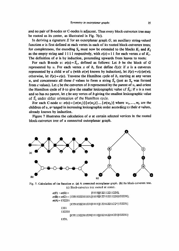
Recall the earlier definition of the block-cutvertex tree of a connected graph. Vertices representing blocks and cutvertices will be termed B-nodes and C-nodes, respectively. Figures 7(a) and 7(b) show a graph and its block-cutvertex tree; in the latter, B-nodes are drawn as solid disks while C-nodes are drawn as empty circles. Now every block-cutvertex tree has a single center, since all its leaves are B-nodes, successive levels in from the leaves consist alternately of all C-nodes and all B-nodes,


and no pair of B-nodes or C-nodes is adjacent. Thus every block-cutvertex tree may be rooted as its center, as illustrated in Fig. 7(c).

In deriving a signature C for an outerplanar graph G, an auxiliary string-valued function o is first defined at each vertex in each of its rooted block-cutvertex trees; for completeness, the encoding S,, must now be extended to the blocks K, and K2 as the empty string and 1 1 1 1 respectively, with C(X) = 1 1 for each vertex x of K2. The definition of cr is by induction, proceeding upwards from leaves to roots:

For each B-node U: O(U) = Sz, defined as follows: Let b be the block of G represented by U. For each vertex x of b, first define E(x): if x is a cutvertex represented by a child w of v (with o(w) known by induction), let e(x) = c(x)cr( w); otherwise, let e(x) = c(x). Traverse the Hamilton cycle of 6, starting at any vertex u, and concatenate all these E values to form a string SU (just as S, was formed from c values). Let z be the cutvertex of b represented by the parent of v, and orient the Hamilton cycle of b to give the smaller lexicographic value of Sz; if v is a root and so has no parent, let z be any vertex of b giving the smallest lexicographic value of Sz under either orientation of the Hamilton cycle.

For each C-node v: a(v)= [ a(~,)] [ o(w2)] . . . [a(~)] where htl, . . . . wk are the children of v, arranged in increasing lexicographic order according to their cr values, already known by induction.

Figure 7 illustrates the calculation of o at certain selected vertices in the rooted block-cutvertex tree of a connected outerplanar graph.

Fig. 7. Calculation of the function CT. (a) A connected outerplanar graph. (b) Its block-cutvertex tree. (c) Block-cutvertex tree rooted at center.

a(F) = a(G) = [ill 1][122I 122112211;

a(B)=a(C)= [13311322311331[1111][122B12211221]132231]; a(A)= 132231

[13311322311331[1111][12211221~22~]132231] 1331 132231

[13311322311331[1111][122f12211221]132231] 1331.


Letting o denote the number of connected components in G, its signature C(G) is now defined as:

C(G) = f dr,) I[ N-2) I. .a i dr,) 1

where rl, . . . , r, are the roots of the rooted block-cutvertex trees of G, arranged in increasing lexicographic order according to their o values.

Since C(G) is uniquely determined from the structure of G, isomorphic graphs always produce the same value of C. Conversely, since the structure of G can be fully recovered from C(G), nonisomorphic graphs always produce different values of 2. Thus C is indeed a signature for the class of outerplanar graphs.

Suppose G has n vert’ces, m edges, and /? blocks. The encoding of each block contains four elements for each of its edges; a pair of square brackets then enclose the encoding of each noncenter block, and each of the u connected components. TIJUS IZ(G)I s 4m + 2/3 + 2~ E O(m + n) = O(n), since m E O(n).

Lexicographic sorting arises in computing Q at C-nodes with multiple children and in computing C for disconnected graphs. Now any finite set of strings may be sorted lexicographically in optimal time which is linear in the sum of their lengths [l, $3.21. Nevertheless, computing ct directly from its definition can lead to an Q(n log n)- or even Q(n2)-time algorithm for A’, since the strings being sorted are constantly growing as the computation of o progresses from the leaves of t+e block-cutvertex tree to its root. To restrict this growth in string length and attain an O(n)-time algorithm, an auxiliary compact encoding ct’ is defined as follows. Let u be any vertex in the tree and let w be a general child of 10. If u is a B-node, then o’(u) = o(u) except that o’(w) rather than a(w) is used in its computation. If v is a C-node, then the (T’ values for the entire level cf B-nodes immediately beneath v are first sorted, and the rank of o’(w) in the resulting list, rather than the value of o(w), is used in forming a’(v). The key to achieving efficiency is that, although the values of B are still computed and still increase in length as they propagate up the tree, only their corresponding o’ values actually take part in the sorting process. This compact encoding scheme is similar to that used in [l] to attain a linear-time tree isomorphism test.

Finally, computing CJ at a B-node which is also a tree root involves choosing z so as to minimize & lexicographically. This may be accomplished efficiently by computing $, for any vertex u in the same block, and then using the linear-time algorithm of [5] to find a left cyclic shift of $, yielding a minimum result.

Careful implementation of the above algorithm, in particular the use of pointer relinking to achieve constant-time string concatenation, leads to:

Theorem 5.1. Every n-vertex outerplanar graph has a signature of length O(n), which can be computed in O(n) time and space.

Once a signature has been obtained, a set of graphs is then easily and efficiently partitioned into isomorphism classes by means of a simple lexicographic sort on the signature values, followed by equality tests on adjacent sorted values. Thus:

Symmetry in otrterplanar graphs 27

Theorem 5.2. Every set of outerplanar graphs, having a total of n vertices, can be partitioned into isomorphism classes in O(n) time and space.

The preceding concepts and results apply in general to all outerplanar graphs; in the present context, it is useful to also introduce the following variation:

Definition. A rooted graph is a connected graph with a single distinguished vertex called its root. A rooted isomorphism is an isomorphism between two rooted graphs which maps one root onto the other. A rooted signature is a signature for a class of rooted graphs, abstracting rooted isomorphism.

Consider now a rooted outerplanar graph G with root r. Since G is connected, it has a single block-cutvertex tree T. A rooted signature for G may be obtained by modifying the signature C of the corresponding unrooted graph as follows:

If r is a cutvertex of G: then root T at the C-node representing r, instead of at its center.

If r is not a cutvertex of G: then root T at the B-node u representing the block containing r, instead of at its center, and define a(u) t= $ instead of &, for the previously-defined vertex z.

This indeed produces a rooted signature, since the resulting string fully deter- mines, and is determined by, the structure of G together with its root r. Hence:

Theorem 5.3. Every n-vertex rooted outerplanar graph has a rooted signature of length O(n), which can be computed in O(n) time and space.

Theorem 5.4. Every set of rooted outerplanar graphs, having a total of n vertices, can be partitioned into rooted isomorphism classes in O(n) time and space.

6. Detecting and displaying symmetry in outerplanar graphs

Define an outerplanar symmetry of a graph to be any symmetry which can be displayed in an outerplanar drawing of the graph. Every outerplanar symmetry is clearly a planar symmetry. It follows easily from Theorem 4.3 and Corollary 4.2 that for biconnected outerplanar graphs, every planar symmetry is actually outerplanar. Moreover, for all outerplanar graphs, every planar rotational symmetry is likewise outerplanar, as isomorphic subgraphs which rotate onto one another can always be redrawn in a uniform outerplanar manner without altering the original symmetry. However, in the absence of biconnectivity an outerplanar graph may have a planar axial symmetry which is not outerplanar, as illustrated in Fig. 8. Outerplanarity is clearly a desirable property in drawings of outerplanar graphs, SO in the remainder of this paper only outerplanar symmetries will be considered. Linear algorithms for general planar symmetries of outerplanar graphs have also been found, but these will not be presented here.

28 J. Manning, M.J. Alallah

Fig. 8. Outerplanar graph with nonouterplanar planar axial symmetry.

Let G be a connected outerplanar graph. Its single block-cutvertex tree may be constructed by using Algorithm 2.2. According as the center of this tree is a B-node or a C-node, the graph G is said to be B-centered or C-centered and the block or cutvertex corresponding to this center is called its central block or central cutvertex, respectively. Because of a basic difference between symmetries of B-centered aud C-centered graphs, as explained later, these two cases will be examined separately.

6.1. Case: G is B-centered

Clearly, any symmetry of G must map the ceutral block onto itself, but may permute amongst themselves the remaining subgraphs, which are known as tufts:

Definition. A tuft of a B-centered graph is a maximal connected rooted subgraph which remains when all edges of the central block are removed; the root of a tuft is its single vertex belonging to the central block.

Note that in all outerplanar drawings of a B-centered graph, the cyclic ordering of its tufts clockwise around its central block is fixed, to within a global reversal, since the outerplanar embedding of this block is unique up to a single reflection.

_Wal symmetry in G will generally be increased by the presence of A-tufts, which can straddle potential axes of symmetry:

Definition. An A-tuft of a B-centered graph is a tuft having an axial symmetry which both maps its root onto itself and can be displayed in an ou’erplanar drawing where all other vertices lie on one side of som5 straight line passing through the root.

The second condition here is necessary to ensure that an A-tuft may be drawn symmetrically in the extericr of the central block. A linear algorithm is given later which decides if a tuft is an A-tuft, and if so, constructs a corresponding drawing.

Under any symmetry of G each tuft must either map entirely onto another tuft, with root mapping onto root, or map onto itself, with root remaining fixed. In the former case, there must be a rooted isomorphism between the tufts; in the latter,


unless the symmetry is merely the identity rotation, the tuft must be an A-tuft. Symmetry detection algorithms for B-centered graphs are extensions of those for

biconnected graphs. The basic approach is to take the previous encoding SU of the central block, expand it to produce a new string $, incorporating relevant details of the tufts, and then search for symmetries in $. To construct &, first use the algorithm of Theorem 5.4 to partition the set of tufts into rooted isomorphism classes X 1, . . . , Xp. Let u be any vertex in the central block, let T be the tuft rooted at v, and let Xi be the isomorphism class of T. Now the previous vertex encoding c(v) has even length, so c(v) =cI(v)c2(v) where Icr(v)l = Iq(v)l. Define:

E(v) = I c,w$ii$c~(v), if T is an A-tuft, cd~)$i$c2W, otherwise.

Then for every vertex u in the central block, the string $, is formed in the same manner as SU except that C(v) is now used in place of c(v) for each such vertex v. Note that I$, I E O(n) and that $ can be constructed in O(n) time and space, where n denotes the number of vertices in G.

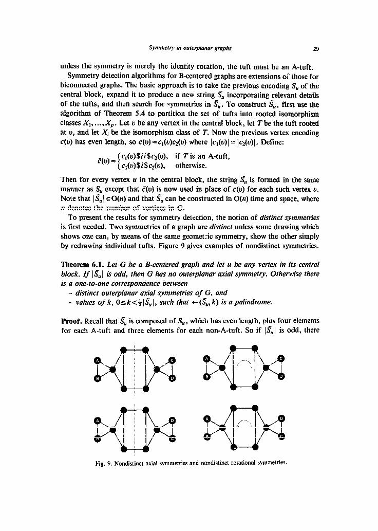
To present the results for symmetry detection, the notion of distinct symmetries is first needed. Two symmetries of a graph are distinct unless some drawing which shows one can, by means of the same geometric symmetry, show the other simply by redrawing individual tufts. Figure 9 gives examples of nondistinct symmetries.

Theorem 6.1. Let G be a B-centered graph and let u be any vertex in its central block. If I Z?,, I is odd, then G has no outer-planar axial symmetry. Otherwise there is a one-to-one correspondence bet ween

- distinct outerplanar axial symmetries of G, and - values of k, 0 I kc + I$], such that + ($, k) is a palindrome.

Proof. Recall that $ is composed of SU , which has even length, plus four elements for each A-tuft and three elements for each non-A-tuft. So if ]$I is odd, there

Fig. 9. Nondistinct axial symmetries and nondistinct rotational symmetries.


must be an odd number of non-A-tufts. In that case no outerplanar drawing of G can have an axis of symmetry, since non-A-tufts must be arranged in matching pairs on opposite sides of any axis, which requires an even number of such tufts.

Otherwise, upon observing that any axial symmetry must map the central block onto itself, the proof of Theorem 3.1 generalizes immediately to establish the stated carrespondence between symmetries and palindromes. Note that since I$1 is even, the middle elements of a palindromic + (&, k) can never be $i $; a configuration of this form would correspond to an axis passing through a non-A-tuft. Cl

Theorem 6.2. Let G be a B-centered graph and let u be any vertex in its central block. Then there is a one-to-one correspondence between

- distinct (outer)planar rotational symmetries of G, a,;d - values of k, Olk<l$[, such that +(&,k)=&

Proof. An immediate generalization of the proof cf Theorem 3.4, upon observing that any rotational symmetry must map the central block onto itself. El

Corollary 6.3. AN distinct outerplanar symmetries of an n-vertex B-centered graph can be enumerated in O(n) time and space.

Proof. Any such graph can possess at most O(n) distinct outerplanar symmetries, each with an O(l)-space description (these axial and rotational symmetries may be specified, respectively, by the vertices and outer edges of the central block which are cut by the axis, and by the number of vertices through which the Hamilton cycle of the central block is rotated). As the proofs of Theorems 6.1 and 6.2 are constructive, the above specifications of the graph symmetries can be recovered directly from the corresponding values of k. These values, in turn, can be enumerated in O(n) time by using Lemmas 3.2 and 3.5 coupled with the KMP algorithm, as before. 0

By contrast, note that there may be Q(2”) nondistinct outerplanar symmetries, as suggested by Fig. 9, each requiring an Q(n)-space description.

To construct a drawing which displays distinct outerplanar axial symmetries of a B-centered graph, start with the regular polygon drawing of its central block (or a single straight-line segment, if this block is &). Then in its exterior, draw each A-tuft symmetrically, as described later, and draw the remaining tufts so that within each rooted isomorphism class, consecutive tufts around the central block are arranged in a mirror-image fashion. Figure 10(a) demonstrates this construction. Using this method, all distinct outerplanar axial symmetries of a B-centered graph can be simultaneously displayed in a single drawing.

Likewise, to display rotational symmetries. start with a similar drawing of the central block. Then in its exterior, draw all the tufts so that within each rooted isomorphism class, each of the tufts is arranged as a rotated copy of its predecessor around the central block. Figure 10(b) demonstrates this construction. Again, using

Symmetry in outerplanar graphs

Fig. 10. Axial and rotational symmetries of a B-centered graph.

this method, all distinct (outer)planar rotational symmetries of a B-centered graph can be simultaneously displayed in a single drawing.

By contrast with the result for biconnected outerplanar graphs (Corollary 4.4), Fig. 10 also shows that in the case of B-centered graphs, it may not be possible to simultaneously display axial and rotational symmetries in the same drawing.

6.2. Case: G is C-centered

Clearly, any symmetry of G must map the central cutvertex onto itself, but may permute amongst themselves the remaining subgraphs, again known as tufts:

Definition. A tuft of a C-centered graph is a maximal connected rooted subgraph which remains when the central cutvertex is removed from the graph and then separately reattached to each of the resulting connected components; the root of each tuft is the central cutvertex.

Recall that in all outerplanar drawings of B-centered graphs, the cyclic ordering of tufts around the central block is essentially fixed. For C-centered graphs, however, the cyclic ordering around the centrai cutvertex is unconstrained. This key difference between B-centered and C-centered graphs has profound implications for symmetry, and explains why the two cases are examined separately here.

Related to this freedom in the placement of tufts is a further difference between B-centered and C-centered graphs: it may not be possible to simultaneously display all distinct outerplanar axial symmetries in a single drawing of a C-centered graph. Such a situation is illustrated by the two drawings of the same graph in Fig. 11. Con- sequently, rather than attempting to find all distinct outerplanar symmetries of a C- centered graph, for the construction of symmetric drawings it is now more appropriate to determine maximum-sized sets of (necessarily distinct) outerplanar symmetries which can be simultaneously displayed in a single drawing.

32 .I. Manning, M.J. Atallah

(a) i 0-d * Fig. 11. Sets of axial symmetries which cannot be displayed simultaneously.

Symmetries of a C-centered graph are essentially those of a single-centered tree, its block-cutvertex tree, refined to take account of the internal structure of its tufts. Results on detection and display of symmetry in trees have already been developed in [12], and are now summarized.

Given a single-centered tree with more than one vertex, its center is removed to yield a set of c-trees, each of which is rooted at the unique vertex previously adjacent to the center. This set is then partitioned into rooted isomorphism classes

Xl , . . . , XP containing N,, . . . , NP trees, respectively. A class Xi is called an A-class if a c-tree from that class, together with the center of the entire tree and the edge joining the center to the root, has itself got an axial symmetry passing through both center and root; in a drawing of the tree, (the root of) a c-tree can lie along an axis of symmetry only if it belongs to an A-class. Letting g = gcd(N,, . . . , NP) and Mi = Ni/g (1 I isp), define the conditions (a) and (p) as follows:

(CX) at most two of the Ni are odd and X’ is an A-class whenever Ni is odd; (8) at most two of the Mi are odd and Xi is an A-class whenever Mi is odd.

Let #A and #a denote the maximum number of axial and rotational symmetries, respectively, which can be simultaneously displayed in single drawings of the tree; their values are then given by:

Theorem 6.4 [12]. #A= 0, if (a) fails; g, if (b) holds; g/2, otherwise.

Theorem 6.5 [ 123. #R = g.

Returning now to C-centered graphs, those tufts which can straddle potential axes of symmetry are again termed A-tufts:

Definition. An A-taft of a C-centered graph is a tuft having an outerplanar axial symmetry which maps its root onto itself.

This definition is somewhat simpler than that for B-centered graphs, as the second condition there is always fulfilled here. Again, a linear algorithm is given later which decides if a tuft is a A-tuft, and if so, constructs a corresponding drawing.

Clearly, the tufts of a C-centered graph are represented by the c-trees of its block- cutvertex tree, with each rooted isomorphism class of A-tufts represented by an


(b)

Fig. 12. Axial and rotational symmetries of a C-centered graph.

A-class of c-trees. Extending the definitions of p, Xi, Ni, g, Mi, (a), (p), #A and #R from trees to C-centered graphs, it follows immediately that:

Theorems 6.4 and 6.5 also hold for C-centered graphs. The proofs of Theorems 6.4 and 6.5 are constructive and provide linear algorithms

which actually produce such maximally-symmetric drawings. For the graph shown in Fig. 12, p = 2, (N,, N2) = (4,4), g = 4, (M,, M2) = (1, l), so (a) holds and (p) fails, giving #A = g/2 = 2 (Fig. 12(a)) and #a = g =4 (Fig. 12(b)). Again, by contrast with the result for biconnected outerplanar graphs (Corollary 4.4), Fig. 12 also shows that in the case of C-centered graphs, it may not be possible to simultaneously display axial and rotational symmetries in the same drawing.

6.3. Recognition and drawing of A-tufts

As already seen, A-tufts play a key role in axial symmetry for both B-centered and C-centered graphs; their efficient detection and display are now examined.

Definition. A plume of a tuft is a maximal connected rooted subgraph which remains when the root is removed from the tuft and then separately reattached to each of the resulting connected components; the root of a plume is the root of its tuft.

Note that a tuft of a B-centered graph may consist of multiple plumes, while a tuft of a C-centered graph always consists of a single plume.

Let T be d tuft of either a B-centered or C-centered graph, and let r be the root of T. Using the algorithm of Theorem 5.4, partition the piumes of T into rooted isomorphism classes, and let q denote the number of odd-sized classes. Then:

l q = 0: T is clearly an A-tuft, and may be drawn symmetrically by arranging the plumes from each class in mirror-image pairs on opposite sides of an axis through r, with all plumes in the same half-plane.

l q = 1: i,et P be a plume from the odd-sized class, and let $- be its encoding,

34 J. Manning, M. J. Atallah

determined recursively. Now T is an A-tuft iff P is itself an A-tuft, which, by a proof similar to those of Theorems 3.1 and 6.1, is true iff I$1 is even and c ($_, 3 Ic(r)l) is a palindrome. Then T may be drawn symmetrically by letting P straddle an axis through r and proceeding as in the case q=O.

l 4 L 2: T is clearly not an A-tuft, since no corresponding symmetric outerplanar drawing is possible in this case.

This now completes the study of symmetry detection and display in connected outerplanar graphs. In the disconnected case, algorithms were also obtained to detect global symmetries and display them in a single drawing of the entire graph, although their complexities are super-linear. However, this global approach seems inappropriate for purposes of conveying structural information about the graph; if some connected components are isomorphic, it appears better to indicate this fact explicitly rather than rely on visual clues to suggest it. The algorithm of Theorem 5.2 may be used to partition the components into isomorphism classes, and a single representative from each class may be analyzed and drawn using the techniques already described. The entire graph may then be displayed either by drawing a single component for each class and indicating its multiplicity, or by replicating the drawings for each component in each class.

Acknowledgement

This author’s research was supported by the Office of Naval Research under con- tracts N00014-84-K-0502 and N00014-86-K-0689, the Air Force Office of Scientific Research under grant AFOSR-90-0107, the National Science Fdundation under grant DCR-845 1393, and the National Library of Medicine under grant ROl-LMO5118.

References

[l] A. Aho, J. Hopcroft and J. Ullman, The Design and Analysis of Computer Algorithms (Addison- Wesley, Reading, MA, 1974).

[2] M.3. Atallah, On symmetry detection, IEEE Trans. Comput. 34 (1985) 663-666. [3] B. Bollobk, Graph Theory: An Introductory Course, Graduate Texts in Mathematics 63 (Springer,

Berlin, 1979). [4] 1 Bondy and U. Murty, Graph Theory with Applications (MacMillan, London, 1976). [S] K. Booth, Lexicographically least circular substrings, Inform. Process. Lett. 10 (1980) 240-242. [6] C. Colbourn and K. Booth, Linear time automorphism algorithms for trees, interval graphs, and

planar graphs, SIAM J. Comput. 10 (1981) 203-225. [7] 1. F&y, On straight line representation of planar graphs, Acta Sci. Math- (Szeged) 11 (1948)

229-233. [8] F. Harary, Graph Theory (Addison-Wesley, Reading, MA, 1969). [9] P. Highnam, Optimal algorithms for finding the symmetries of a planar point set, Inform. Process.

Lett. 22 (1986) 219-222. El01 D. Knuth, J. Morris and V. Pratt, Fast pattern matching in strings, SIAM J. Comput. 6 (1977)

323-350.


[1 I] J. Manning, Computational complexity of geometric symmetry detection in graphs, Lecture Notes in Computer Science 507 (Springer, Berlin, 1991) l-7.

[12] J. Manning and M.J. Atallah, Fart detection and display of symmetry in trees, Congr. Numer. 64 (1988) 159-169.

[13] S. Mitchell, Linear algorithms to recognize outerplanar and maximal outerplanar graphs, Inform. Process. Lett. 9 (1979) 229-232.

[14] M. Sydo, Outerplanar graphs: Characterizations, testing, coding, and counting, Bull. Acad. Polon. Sci. Ser. Sci. Math. Astron. Phys. 26 (1978) 675-684.

[ 151 J. Wolter, T. Woo and R. Volz, Optimal algorithms for symmetry detection in two and three dimen- sions, The Visual Computer 1 (1985) 37-48.

fast detection and display of symmetry in outerplanar graphs

Documents