Fast Generation of Large Scale Social Networks withClustering

Joseph J. Pfeiffer III, Timothy La Fond, Sebastian Moreno, Jennifer NevillePurdue University

Department of Computer ScienceWest Lafayette, IN

{jpfeiffer, tlafond, smorenoa, neville}@purdue.edu

ABSTRACTA key challenge within the social network literature is theproblem of network generation – that is, how can we createsynthetic networks that match characteristics traditionallyfound in most real world networks? Important characteris-tics that are present in social networks include a power lawdegree distribution, small diameter and large amounts ofclustering; however, most current network generators, suchas the Chung Lu and Kronecker models, largely ignore theclustering present in a graph and choose to focus on preserv-ing other network statistics, such as the power law distribu-tion. Models such as the exponential random graph modelhave a transitivity parameter, but are computationally dif-ficult to learn, making scaling to large real world networksintractable.

In this work, we propose an extension to the Chung Lu ran-dom graph model, the Transitive Chung Lu (TCL) model,which incorporates the notion of a random transitive edge.That is, with some probability it will choose to connect toa node exactly two hops away, having been introduced toa ‘friend of a friend’. In all other cases it will follow thestandard Chung Lu model, selecting a ‘random surfer’ fromanywhere in the graph according to the given invariant dis-tribution. We prove TCL’s expected degree distribution isequal to the degree distribution of the original graph, whilebeing able to capture the clustering present in the network.The single parameter required by our model can be learnedin seconds on graphs with millions of edges, while networkscan be generated in time that is linear in the number ofedges. We demonstrate the performance TCL on four real-world social networks, including an email dataset with hun-dreds of thousands of nodes and millions of edges, showingTCL generates graphs that match the degree distribution,clustering coefficients and hop plots of the original networks.

Categories and Subject DescriptorsG.2.2 [Graph Theory]: Network problems; G.3 [Probabilityand Statistics]: Markov processes

1. INTRODUCTIONA challenging problem within the social network commu-nity is generating graphs which adhere to certain statistics.Due to the prevalence of ‘small world’ graphs such as Face-book and the Internet [16], models which attempt to captureproperties of small world graphs such as a power law de-gree distribution, small diameter and clustering greater thanrandomly present for the sparsity of the network have be-come a much-discussed topic in the field [7, 13, 3, 10, 2, 14].The first random graph model, the Erdos-Renyi model[4],proposed random connections between nodes in the graphwhere each edge is sampled independently; however, thismodel has a Binomial degree distribution, not power law,and generally lacks clustering when generating sparse net-works. As a result, multiple attempts have been made todevelop algorithms that generate graphs with small worldnetwork properties.

Exponential Random Graph Models (ERGM) extend theErdos-Renyi model to allow additional statistics of the graphas parameters [13]. The typical approach is to model the net-work under the assumption of Markov independence through-out the graph – edges are only dependent on other edges thatshare the same node . Using this, ERGMs define an expo-nential family of models using various Markov statistics ofthe graph, allowing for the incorporation of a transitivityparameter, then maximize the likelihood of the parametersgiven the graph. The algorithms for learning and generatingERGMs are resource intensive and intractable for applica-tion to networks of more than a few thousand nodes.

As a result, newer efforts make scaleability an explicit goalwhen constructing models and algorithms. Notable exam-ples include the Chung-Lu Graph Model (CL) [3] and theKronecker Product Graph Model (KPGM) [7]. CL is alsoan extension of the Erdos-Renyi model, but rather than cre-ating a summary statistic based on the degrees, it gener-ates a new graph such that the expected degree distributionmatches the given distribution exactly. In contrast, KPGMlearns a 2x2 matrix of parameters and lays down edges ac-cording to the Kronecker product of the matrix to itself logntimes. For large graphs this algorithm can learn the param-eters defined by the 2x2 matrix in hours and can generatelarge graphs in minutes.

With CL and KPGM we have scalable algorithms for learn-ing and generating graphs with hundreds of thousands ofnodes and millions of edges. However, in order to achieve

arX

iv:1

202.

4805

v1 [

cs.S

I] 2

2 Fe

b 20

12

scalability, a power law degree distribution and small diame-ter, both models have made the decision to ignore clusteringin their generated graphs. This is not an insignificant con-sequence, as a small world network is in part defined by theclustering of nodes [16]. While ERGM can potentially learnnetworks with clustering, the complexity of the model makesit a poor prospect when considering learning and generatinggraphs with massive size.

In order to generate sparse networks which can accuratelycapture the degree distribution, small diameter and clus-tering, we propose to extend the CL algorithm in multipleways. The first portion of this paper will show how the naivefast generation algorithm for the CL model is biased, andwe develop a correction to this problem. Next, we introducea generalization to the CL model known as the TransitiveChung Lu (TCL). To do this, we observe that the CL modelis a ‘random surfer’ model, similar to the PageRank randomwalk algorithm[9]. However, CL always chooses the randomsurfer and has no affinity for nodes along transitive edges.In contrast, our TCL model will sometimes choose to fol-low these transitive edges and then close a triangle ratherthan selecting a random node according to the surfer. Theprobability of randomly surfing versus closing a triangle is asingle parameter in our model which we can learn in secondsfrom an observed graph, compared to the hours required tolearn KPGM. In short, the contributions in our work can besummarized as follows:

• Introduction of a ‘random triangle’ parameter to theCL model

• A correction to the ‘edge collision’ problem seen innaive fast CL model generation

• Analysis showing TCL has an expected degree distri-bution equal to the original input network’s degree dis-tribution

• A learning algorithm for TCLs that runs in seconds forgraphs with millions of edges

• A generation algorithm for TCLs which runs on thesame order as naive fast CL, and faster than KPGM

• Empirical demonstrations that show the graphs gen-erated from TCL match the degree distribution, clus-tering coefficient and hop plots of the original graphbetter than fast CL or KPGM

In section 2 we discuss in more depth the ERGM, KPGMand CL models, while in section 3 we outline the basis forthe CL model. Next, we show the fast method used forgenerating graphs in section 4, and our correction to it. Insection 5 we introduce our modification to the CL model,proving the expected degree distribution and demonstratinghow to learn the transitive probability, while in section 6 weanalyze the runtimes of our fast CL correction and TCL. Insection 7 we learn the parameter and generate graphs whichclosely match the original graphs. We end in section 8 withconclusions and future directions.

2. RELATED WORKRecently there has been a great deal of work focused on thedevelopment of generative models for small world and scale-free graphs (e.g., [5, 16, 2, 6, 15, 7, 3]). As an example,the Chung Lu model is able to generate a network whichhas a provable expected degree distribution equal to the de-gree distribution of the original graph. The CL model, likemany, attempts to define a process which matches a subsetof features observed in a network.

The importance of the clustering coefficient has been demon-strated by Watts and Strogatz [16]. In particular, they showthat small world networks (including social networks) arecharacterized by a short path length and large clustering co-efficient. One recent algorithm (Seshadri et al [14]) matchesthese statistics by putting together nodes with similar de-grees and generating Erdos-Renyi graphs for each group.The groups are then tied together. However, this algorithmneeds a parameter to be set manually to work. Existingmodels that can generate clustering in the network gener-ally do not have a training algorithm.

One method that can model clustering and can learn the as-sociated parameter is the Exponential Random Graph Model(ERGM) [15]. ERGMs define a probability distribution overthe set of possible graphs with a log-linear model that usesfeature counts of local graph properties. However, thesemodels are typically hard to train as each update of theFisher scoring function takes O(n2). With real-world net-works numbering in the hundreds of thousands if not millionsof nodes, this makes ERGMs impossible to fit.

Another method is the Kronecker product graph model (KPGM),a scalable algorithm for learning models of large-scale net-works that empirically preserves a wide range of global prop-erties of interest, such as degree distributions, and path-length distributions [7]. Thanks to these characteristics,KPGM has been selected as a generation algorithm for theGraph 500 Supercomputer Benchmark [10].

The KPGM starts with a initial square matrix Θ1 of sizeb × b, where each cell value is a probability. To generatea graph, the algorithm uses k Kronecker multiplications togrow until a determined size (obtaining Θk with bk = N rowsand columns). Each edge is then independently sampledusing a Bernoulli distribution with parameter Θk(i, j). Arough implementation of this algorithm has time O(N2), butimproved algorithms can generate a network in O(M logN),where M is the number of edges in the network [7]. Accord-ing to [7], the learning time is linear in the number of edges.

3. CHUNG-LU MODEL AND INVARIANTMC DISTRIBUTION

Define graph G = 〈V,E〉, where V is a set of N vertices, ornodes, and E = V × V is a set of M edges or relationshipsbetween the vertices. Let A represent the adjacency matrixfor G where:

Aij =

{1 if E contains the tuple (vi, vj)

0 otherwise(1)

Next, define the diagonal matrix D such that:

Dij =

{∑k Aik if i = j

0 otherwise(2)

The diagonal of matrix D represents the degree of each node,where Dii is the degree of node i. Finally, define the transi-tion probability matrix P :

Pij =Aij

Dii(3)

This transition probability matrix is the probability of ar-riving at any node during a random walk that is uniformover the edges. It is important to note that the rows of Pare normalized:

∑j

Pij =∑j

Aij

Dii=

1

Dii

∑j

Aij =Dii

Dii= 1 (4)

3.1 Chung Lu ModelThe Chung Lu model assigns edges to the graph by indepen-dently laying edges for each possible edge with probability:

DiiDjj

2M

It is assumed Dkk <√M ∀k. The expected degree distri-

bution for this graph is simply:

EG[DCLii ] =

∑j

DiiDjj

2M= Dii

∑j

Djj

2M= Dii

3.2 Fast Chung Lu ModelThe invariant distribution of a graph is the distribution thatwhen multiplied with the transition probability matrix re-turns itself:

π ∗ P = π

A possible candidate for such a distribution is defined interms of the degrees of the network, where π(i) = Dii

2M:

π(i) =∑j

π(j) ∗ Pji =∑j

Djj

2M· Aji

Djj=∑j

Aji

2M=Dii

2M

If we assume the matrix P is stationary (not changing as therandom walker steps through the graph) and non-bipartite,the π distribution is unique and tends to the stationary dis-tribution π as the number of steps tends to infinity [8].

In [10], the authors describe a fast edge-laying algorithmwhich runs in O(M). The algorithm proceeds by creating avector of size O(M), then places the IDf of each node vi inthe vector Dii times. It is not hard to see that since the sumof the degrees equals the number of edges in the graph, eachnode can place its ID exactly Dii times without collision,and without leaving empty space in the vector.

Next, a node ID vi is drawn from the vector – this can bedone in O(1) by drawing a uniform random variable between

Algorithm 1 CL(π,N, |E|)1: ECL = {}2: initialize(queue)3: for iterations do4: if queue is empty then5: vj = pi sample(π)6: else7: vj = pop(queue)8: end if9: vi = pi sample(π)

10: if eij 6∈ ECL then11: ECL = ECL ∪ eij12: else13: push(queue, vi)14: push(queue, vj)15: end if16: end for17: return(ETCL)

1 and M , and using offsets to index into the array. Thenext step is to draw another independent vertex vj from thevector and place the edge between the two sampled nodes.In a special graph, the regular graph, we can show that theprobability of an edge existing is exactly the same for thefast CL method and the slow.

Proposition 1. In a regular graph, the probability of anedge existing in the Fast Chung-Lu model is the same as theprobability of an edge existing in the Slow Chung-Lu Model.

Proof. Let vi, vj be two nodes in our network. Accord-ing to the Fast Chung Lu model we will select every node atrandom with replacement, meaning the number of times thenode vj will be selected as the first node is Dj , where D isthe degree for every node in the network, and j is used fornotation, to indicate the particular node. Since this graphis regular, Di = Dj ∀i, j. The probability of an edge beingplaced from vj to vi is the sum:

P (eij |vj) =Di

2M+

∑vk∈V,k 6=i

Dk

2M

Di

2M − Dk

+ . . .

=Di

2M+

Di

2M

∑vk∈V,k 6=i

Dk

2M − Dk

+ . . .

=Di

2M+

Di

2M

2M − Di

2M − Dk

+ . . .

= 2Di

2M

(5)

The sum continues to Dj . The probability of inserting onthe d insertion is therefore:

=∑vk1

Dk

2M

∑vk2

Dk2

2M − D· · ·

∑vkd

Dkd

2M − (d− 1)D

Di

2M − dD

=Di

2M

∑vk1

Dk1

2M − D

∑vk2

Dk2

2M − 2D· · ·

∑vkd

Dkd

2M − dD

=Di

2M

(6)

10-3 10-2 10-1 100

Chung Lu Expected Proportion

10-3

10-2

10-1

100

Act

ual Pro

port

ion

Fast CL Edge Probabilities

PerfectTop-Original

(a) Original

10-3 10-2 10-1 100

Chung Lu Expected Proportion

10-3

10-2

10-1

100

Act

ual Pro

port

ion

Fast CL Edge Probabilities

PerfectTop-RandomTop-Top

(b) Adjusted

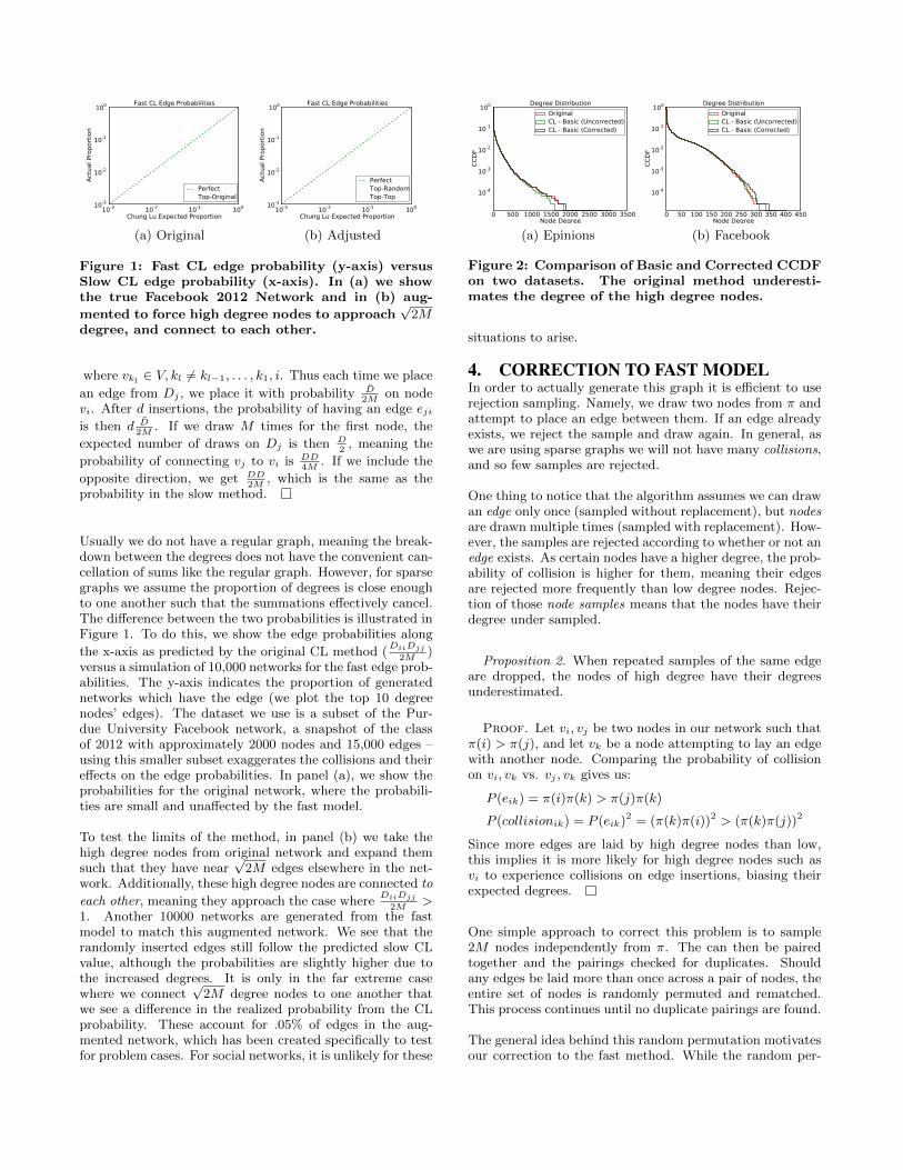
Figure 1: Fast CL edge probability (y-axis) versusSlow CL edge probability (x-axis). In (a) we showthe true Facebook 2012 Network and in (b) aug-

mented to force high degree nodes to approach√

2Mdegree, and connect to each other.

where vkl ∈ V, kl 6= kl−1, . . . , k1, i. Thus each time we place

an edge from Dj , we place it with probability D2M

on nodevi. After d insertions, the probability of having an edge ejiis then d D

2M. If we draw M times for the first node, the

expected number of draws on Dj is then D2

, meaning the

probability of connecting vj to vi is DD4M

. If we include the

opposite direction, we get DD2M

, which is the same as theprobability in the slow method.

Usually we do not have a regular graph, meaning the break-down between the degrees does not have the convenient can-cellation of sums like the regular graph. However, for sparsegraphs we assume the proportion of degrees is close enoughto one another such that the summations effectively cancel.The difference between the two probabilities is illustrated inFigure 1. To do this, we show the edge probabilities along

the x-axis as predicted by the original CL method (DiiDjj

2M)

versus a simulation of 10,000 networks for the fast edge prob-abilities. The y-axis indicates the proportion of generatednetworks which have the edge (we plot the top 10 degreenodes’ edges). The dataset we use is a subset of the Pur-due University Facebook network, a snapshot of the classof 2012 with approximately 2000 nodes and 15,000 edges –using this smaller subset exaggerates the collisions and theireffects on the edge probabilities. In panel (a), we show theprobabilities for the original network, where the probabili-ties are small and unaffected by the fast model.

To test the limits of the method, in panel (b) we take thehigh degree nodes from original network and expand themsuch that they have near

√2M edges elsewhere in the net-

work. Additionally, these high degree nodes are connected to

each other, meaning they approach the case whereDiiDjj

2M>

1. Another 10000 networks are generated from the fastmodel to match this augmented network. We see that therandomly inserted edges still follow the predicted slow CLvalue, although the probabilities are slightly higher due tothe increased degrees. It is only in the far extreme casewhere we connect

√2M degree nodes to one another that

we see a difference in the realized probability from the CLprobability. These account for .05% of edges in the aug-mented network, which has been created specifically to testfor problem cases. For social networks, it is unlikely for these

0 500 1000 1500 2000 2500 3000 3500Node Degree

10-4

10-3

10-2

10-1

100

CC

DF

Degree Distribution

OriginalCL - Basic (Uncorrected)CL - Basic (Corrected)

(a) Epinions

0 50 100 150 200 250 300 350 400 450Node Degree

10-4

10-3

10-2

10-1

100

CC

DF

Degree Distribution

OriginalCL - Basic (Uncorrected)CL - Basic (Corrected)

(b) Facebook

Figure 2: Comparison of Basic and Corrected CCDFon two datasets. The original method underesti-mates the degree of the high degree nodes.

situations to arise.

4. CORRECTION TO FAST MODELIn order to actually generate this graph it is efficient to userejection sampling. Namely, we draw two nodes from π andattempt to place an edge between them. If an edge alreadyexists, we reject the sample and draw again. In general, aswe are using sparse graphs we will not have many collisions,and so few samples are rejected.

One thing to notice that the algorithm assumes we can drawan edge only once (sampled without replacement), but nodesare drawn multiple times (sampled with replacement). How-ever, the samples are rejected according to whether or not anedge exists. As certain nodes have a higher degree, the prob-ability of collision is higher for them, meaning their edgesare rejected more frequently than low degree nodes. Rejec-tion of those node samples means that the nodes have theirdegree under sampled.

Proposition 2. When repeated samples of the same edgeare dropped, the nodes of high degree have their degreesunderestimated.

Proof. Let vi, vj be two nodes in our network such thatπ(i) > π(j), and let vk be a node attempting to lay an edgewith another node. Comparing the probability of collisionon vi, vk vs. vj , vk gives us:

P (eik) = π(i)π(k) > π(j)π(k)

P (collisionik) = P (eik)2 = (π(k)π(i))2 > (π(k)π(j))2

Since more edges are laid by high degree nodes than low,this implies it is more likely for high degree nodes such asvi to experience collisions on edge insertions, biasing theirexpected degrees.

One simple approach to correct this problem is to sample2M nodes independently from π. The can then be pairedtogether and the pairings checked for duplicates. Shouldany edges be laid more than once across a pair of nodes, theentire set of nodes is randomly permuted and rematched.This process continues until no duplicate pairings are found.

The general idea behind this random permutation motivatesour correction to the fast method. While the random per-

mutation of all 2M nodes is somewhat extreme, a methodwhich permutes only a few edges in the graph – the oneswith collisions – is feasible. With this in mind, our solutionto this problem is straightforward. Should we encounter acollision, we place both vertices in a waiting queue. Beforecontinuing with regular insertions we will attempt to selectneighbors for all nodes in the waiting queue. Should the newedge for a node in the queue also encounter a collision, thechosen neighbor is also placed in the queue, and so forth.This ensures that if a node is ‘due’ for a new edge but isprevented from receiving it due to a collision, the node is‘slightly permuted’ by exchanging places with a node sam-pled later.

This shuffling ensures thatM edges actually be placed, whichis needed by proposition 1, without affecting the degree dis-tribution as can happen by proposition 2. Furthermore, aswe leave an edge if it ever occurs, the probability defined byproposition 1 is never lowered for the edges which have mul-tiple occurrences, only raised to ensure M edges are placed.

Our correction to the fast CL model assumes independencebetween the edge placements and the current graph config-uration. This independence only truly holds when collisionsare allowed (i.e. when generating a multigraph). In practiceedge placements are not truly independent, as we disallowthe placement of edges that already exist in the graph. Thecorrection we have described removes the bias described inproposition 2 but is not guaranteed to generate graphs ex-actly according to the original π distribution. The fast ver-sion of the graph generation algorithm must project from aspace of multigraphs down into a space of simple graphs, andthis projection is not necessarily uniform over the space ofgraphs. However, our empirical results show that on sparsegraphs our correction removes the majority of the bias dueto collisions and that the bias from the projection is negli-gible, meaning we can treat graphs form the corrected fastgeneration as being drawn from the original Chung-Lu graphdistribution. While the slow Chung-Lu model is guaranteedto produce unbiased π distributed graphs, the fast methodproduces graphs which are nearly indistinguishable from theslow method and runs an order of magnitude faster.

In Figure 2, we can see the effect of the correction on twolabeled datasets, Epinions and Facebook (described in sec-tion 7). The green line corresponding to the simple inser-tion technique underestimates the degrees of the high degreenodes in both instances. The correction results in having amuch closer match on the high degree nodes. By utilizingthis correction, we can generate graphs whose degree distri-butions are unaffected by the possibility of collision and areable to generate graphs in O(M).

5. TRANSITIVE CHUNG-LU MODELA large problem with the Chung-Lu model is the lack oftransitivity captured by the model. As many social net-works (among others) are formed via friendships, drawingrandomly from distribution of nodes across the network failsto capture this property. We propose the Transitive ChungLu model described in algorithm 2, which has a probabilityof a ‘random surfer’ connecting two nodes across the net-work but has an additional probability of creating a newtransitive edge across a pair of nodes connected by a 2 hop

Algorithm 2 TCL(π, ρ,N, |E|, iterations)1: ETCL = CL(π,N, |E|)2: initialize(queue)3: for iterations do4: if queue is empty then5: vj = pi sample(π)6: else7: vj = pop(queue)8: end if9: r = bernoulli sample(ρ)

10: if r = 1 then11: vk = uniform sample(ETCL

j )

12: vi = uniform sample(ETCLk )

13: else14: vi = pi sample(π)15: end if16: if eij 6∈ ETCL then17: ETCL = ETCL ∪ eij18: // remove oldest edge from ETCL

19: ETCL = ETCL \min(time(ETCL))20: else21: push(queue, vi)22: push(queue, vj)23: end if24: end for25: return(ETCL)

path. The CL model is now a special case of TCL whereρ = 0 and edge selection is always done through a randomwalk. In the TCL model, we include the transitive edgeswhile maintaining the same expected invariant distributionas the CL model. Thus the TCL model is guaranteed tohave an expected degree distribution equal to that of theoriginal network.

We begin by constructing a graph of M edges using thestandard Chung-Lu model as described above. This givesus an initial edge set E which has the same expected degreedistribution as the original data. We then initialize a queuewhich will be used to store nodes that have a higher prior-ity for receiving an edge. Next, we define an update stepwhich replaces the oldest edge in the graph with a new oneselected according to the TCL model and repeat this processfor the specified number of iterations. If the priority queueis not empty, we will choose the next node in the queue tobe vj , the first endpoint of the edge; otherwise, on line 5we sample vj using the π distribution. With probability ρwe will add an edge between vj and some node vi throughtransitive closure by choosing an intermediate node vk uni-formly from j’s neighbors, then selecting vi uniformly fromk’s neighbors. In contrast, with probability (1 − ρ) we usethe ’random surfer’ method by randomly choosing vi fromthe graph according to the invariant distribution π.

Either method, transitive or random surfer, returns an ad-ditional node to the method to use as the other endpoint.If the selected edge is not already part of the graph, we willadd it and remove the oldest edge in the graph (continuallyremoving the warmup CL edges). If the selected edge is al-ready present in the graph, we place the selected endpointnodes into the priority queue (lines 21 and 22). We repeat

this replacement operation many times to ensure that theoriginal graph is mostly replaced and then return the set ofedges as the new graph. In practice, we find that M replace-ments – enough to remove all edges generated originally byCL – is sufficient.

In order to show that this update operation preserves theexpected degree distribution, we prove the following:

1. From any starting point vj the probability of a twohop walk ending on node vi is π(i)

2. The probability that TCL selects an edge eij is thesame as CL selecting eij

3. The change in the expected degree distribution after aTCL iteration is zero

As the graph is initialized to a CL that has expected degreedistribution equal to the original graph, and updates are per-formed that that preserve the expected degree distribution,the final graph will have the same expected degree distri-bution through induction. Our update step is a stochasticcombination of two edge insertion operations: one that sam-ples an edge using the π distribution as in the standard CLmodel, and one that samples an edge based on 2 hop paths.Naturally the CL insertion select edges based on the π dis-tribution by definition. Now we will show that samplingan edge using the existing 2 hop paths also selects edgesaccording to the π distribution.

Theorem 1. Starting from any node vj , if the edges in thegraph are distributed according to π(k)π(i) and the walkertraverses two hops by sampling uniformly over the edgesof vj and subsequently the selected neighbor vk of vj , theprobability of ending this walk on node vi is π(i).

Proof. We can represent the probability of a particularpath vj → vk → vi existing in the graph as

P (pathjki) =DjjDkk

2M

DkkDii

2M(7)

The probability of following this path in a uniform randomwalk in the CL graph, when it exists, is:

P (walkjki) =1

DCLj DCL

k

(8)

To calculate the probability of a walk starting on node j andending at node i, we have to normalize by the probabilityof walking a 2 hop path from node j to any other node i′ in

the graph:

P (walkji) =

∑k∈V P (pathjki) · P (walkjki)∑

i′∈V∑

k∈V P (pathjki′) · P (walkjki′)

=

∑k∈V

DjjDkk

2MDkkDii

2M1

DCLj DCL

k∑i′∈V

∑k∈V

DjjDkk

2M

DkkDi′i′2M

1DCL

j DCLk

=

∑k∈V DjD

2kDi

1DCL

j DCLk∑

i′∈V∑

k∈V DjD2kDi′

1DCL

j DCLk

=

∑k∈V DkDi

1DCL

k∑i′∈V

∑k∈V DkDi′

1DCL

k

=Di

∑k∈V Dk

1DCL

k∑i′∈V Di′

∑k∈V Dk

1DCL

k

=Di∑

i′∈V D′i

=Di

2M= π(i)

So regardless of the starting node j, the probability of land-ing on i after traveling 2 hops uniformly over the edges isπ(i).

Utilizing the above theorem, we next show the probabilityof an edge eij existing in the graph is π(j)π(i).

Theorem 2. The Transitive Chung-Lu model selects edgeeij for insertion with probability

P (eij) = π(i) ∗ π(j) (9)

Proof. The inductive step randomly selects a node vjfrom the invariant distribution π to be the first endpointof a new edge. From vj , we have two options to completethe edge: with probability ρ we use the transitive closure towalk 2 hops to find the other endpoint, and with probability1 − ρ we perform a random surf using π. The invariantdistribution for πTCL(i) can then be written as:

πTCL(i) =∑j

π(j) [ρ ∗ P (walkji) + (1− ρ)π(i)]

In theorem 1 we showed that P (walkji) = π(i). Now theprobability of selecting edge eij can be written as:

P (eij) = π(j) ∗ πTCL

= π(j) ∗ (ρ ∗ π(i) + (1− ρ) ∗ π(i))

= π(j) ∗ π(i)

Therefore, the inductive step of TCL will place the endpointsof the new edge according to π.

Corollary 1. The expected degree distribution of the graphproduced by TCL is the same as the degree distribution ofthe input graph.

Proof. The inductive step of TCL places an edge withendpoints distributed according to π, so the expected in-crease in the degree of any node vi is π(i). However, the in-ductive step will also remove the oldest edge that was placedinto the network. Since the oldest edge can only have beenplaced in the graph through a Chung-Lu process or a transi-tive closure, the expected decrease in the degree is also π(i),which means the expected change in the degree distributionis zero. Because the CL initialization step produces a graphwith expected degree distribution equal to the input graph’sdistribution, and the TCL update step causes zero expectedchange in the degree distribution the output graph of theTCL algorithm has expected degree distribution equal tothe input graph’s distribution by induction.

This means we are placing edges according to π(i)π(j), anddoing M insertions. This is the same model as shown forthe fast CL method, which also inserts M edges accordingto π(i)π(j), meaning that if the fast CL method follows slowCL, TCL does as well. In practice, TCL and CL capture thedegree distribution well (section 7).

5.1 Fitting Transitive Chung LuNow that we have introduced a ρ parameter which controlsthe proportion of transitive edges in the network we needa method for learning this parameter from the original net-work. For this, we need to estimate the probability ρ bywhich edge formation is done by triadic closure, and theprobability 1 − ρ by which the random surfer forms edges.We can accomplish this estimation using an ExpectationMaximization algorithm. First, let zij ∈ Z be latent vari-ables on each eij ∈ E with values zij ∈ {1, 0}, where 1indicates the edge eij was laid by a transitive closure and 0indicates the edge was laid by a random surfer. Althoughthe Z values are unknown we can jointly estimate them withρ using EM.

We can now define the conditional probability of placing anedge eij from starting node vj given the method zij by whichthe edge was placed:

P(eij |zij = 1, vj , ρ

t) =ρt∑

vk∈ej∗

I[vi ∈ ek∗]Djj

1

Dkk

P(eij |zij = 0, vj , ρ

t) =(1− ρt) · π(i)

Given the starting node vj , the probability of the edge exist-ing between vi and vj , given that the edge was placed dueto a triangle closure is ρ times the probability of walkingfrom vj to a mutual neighbor of i and j and then continuingthe walk on to i, while 1− ρ is the probability the edge wasplaced by a random surfer. We now show the EM algorithm.

ExpectationNote that the conditional probability of zij , given the edgeeij and ρ, can be defined in terms of the probability of an

0.0 0.5 1.0 1.5 2.0 2.5 3.0 3.5 4.0Iteration

0.0

0.2

0.4

0.6

0.8

1.0

Curr

ent

Est

imate

d R

ho

Convergence Rate

EpinionsFacebookGnutella30PurdueEmail

(a)

0.0 0.5 1.0 1.5 2.0 2.5 3.0 3.5Time (seconds)

0.0

0.2

0.4

0.6

0.8

1.0

Curr

ent

Est

imate

d R

ho

Convergence Rate

EpinionsFacebookGnutella30PurdueEmail

(b)

Figure 3: Convergences of the EM algorithm – bothin terms of time and number of iterations. 10000samples per iteration.

edge being selected by the triangle closure divided by theprobability of the edge being laid by any method. UsingBayes’ Rule, our conditional distribution on Z is simply:

P(zij = 1|eij , vj , ρt

)=

ρt[∑

vk∈ej∗I[vi∈ek∗]

Djj

1Dkk

]ρt[∑

vk∈ej∗I[vi∈ek∗]

Djj

1Dkk

]+ (1− ρt) [π(i)]

And our expectation of zij is

E[zij |ρt] = P(zij = 1|eij , vj , ρt

)MaximizationTo maximize this expectation, we note that ρ is a Bernoullivariable representing P (zij = 1). We sample a set of edges Suniformly from the graph to use as evidence when updatingρ. The variables zij are conditionally independent given theedges and nodes in the graph, meaning the MLE update toρ is then calculating the expectation of zij ∈ S and thennormalizing over the number of edges in S:

ρt+1 =1

|S|∑zij∈S

E[zij |ρt]

The method we used to sample these edge subsets was toselect them uniformly from the set of all edges. This canbe done quickly using the node ID vector we constructedfor sampling from the π distribution. As any node i ap-pears Di times in this vector, sampling a node from thevector and then uniformly sampling one of its edges gives usa Di

M∗ 1

Di= 1

Mprobability of sampling any given edge. We

gathered subsets of 10000 edges per iteration and our EMalgorithm converges in just a few seconds, even on datasetswith millions of edges. Figure 3 shows the convergence timeon each of the datasets.

6. TIME COMPLEXITYThe methods presented for both generating a new networkand for learning the parameter ρ can be done in an efficientmanner.

First, we need to bound the expected number of attemptsto insert an edge into the graph. Note that a node vi with

c edges has probability π(i) = cM

of hitting its own edgeon the draw from π; by extension, the probability of hittingits own edges k times is π(i)k. This represents a geometricdistribution which has the expected value of hits H on theedges of the nodes being:

E [H|π(i)] = (1− π(i))∑k=1

π(i)k−1 =1

1− π(i)

This shows the expected number of attempts to insert anedge is bounded by a constant. As a result, we can gener-ate the graph in O(N +M), the same complexity as ChungLu. The initial steps of initializing our vector of node idsand running the basic CL model takes O(N +M). Next, weneed to generate M insertions while gradually removing thecurrent edges. This can be seen in lines 3-24 of Algorithm 2.In this loop, the longest operations are selecting randomlyfrom neighbors or removing an edge. Both of these opera-tions cost is in terms of the maximum degree of the network,which we assumed bounded, meaning those operations canbe done in O(1) time. As a result, the total runtime of graphgeneration is O(N +M).

For the learning algorithm, assume we have I iterationswhich gather s samples. It is O(1) to draw a node from thegraph and O(1) to choose a neighbor, meaning each iterationcosts O(s). Coupled with the cost of creating the initial πsampling vector, the total runtime is then O(N +M + I · s).

7. EXPERIMENTSFor our experiments, we compared three different graphgenerating models. The first is the fast Chung Lu (CL)generation algorithm with our correction for the degree dis-tribution. The second is Kronecker Product Graph Model(KPGM) implemented with code taken from the SNAP li-brary1 calculated by the authors[7]. Lastly, we compared theTransitive Chung Lu (TCL) method presented in this paperusing the EM technique to estimate the ρ parameter. Allexperiments were performed in Python on a Macbook Pro,aside from the KPGM parameters which were generated ona desktop computer using C++2. All of these networks weremade undirected by reflecting the edges in the network, ex-cept for the Facebook network which is already undirected.

7.1 DatasetsTo empirically evaluate the models, we learned model pa-rameters from real-world graphs and then generated newgraphs using those parameters. We then compared the net-work statistics of the generated graphs with those of theoriginal networks. The four networks used are all large so-cial networks, and their node and edge counts can be foundin Figure 4.a.

The first dataset we analyze is the Epinions dataset [11].This network represents the users of Epinions, a websitewhich encourages users to indicate other users whose con-sumer product reviews they ‘trust’. The reviews of all userson a product are then weighted to incorporate both the re-viewer ratings and the amount of trust received from other

1SNAP: Stanford Network Analysis Project. Available athttp://snap.stanford.edu/snap/index.html2SNAP is written in C++

users. The edge set of this network represents nominationsof trustworthy individuals between the users.

Next, we study the collection of Facebook friendships fromthe Purdue University Facebook network. In this network,the users can add each other to their lists of friends and sothe edge set represents a friendship network. This networkhas been collected over a series of snapshots for the past4 years; we use nodes and friendships aggregated across allsnapshots.

The Gnutella30 network is a different type than the othernetworks presented. Gnutella is a Peer2Peer network whereusers are attempting to find seeds for file sharing [12]. Theuser reaches out to its current peers, querying if they have afile. If not, the friend refers them to other users who mighthave a file, repeating this process until a seed user can befound. Because this network represents the structure of afile sharing program rather than true social interactions, ithas significantly less clustering than the other networks.

Lastly, we study a collection of emails gathered from theSMTP logs of Purdue University [1]. This dataset has anedge between users who sent e-mail to each other. The mail-ing network has a small set of nodes which sent out mail ata vastly greater rate than normal nodes; these nodes weremost likely mailing lists or automatic mailing systems. Inorder to correct for these ‘spammer’ nodes, we remove nodeswith a degree greater than 1, 000 as these nodes did not rep-resent participants in any kind of social interaction. Thenetwork has over two hundred thousand nodes, and nearlytwo million edges (Figure 4.a).

7.2 Running TimeIn Figure 3 we can see the convergence of the EM algorithmwhen learning parameter ρ, both in terms of the number ofiterations and in terms of the total clock runtime. Due tothe independent sample sets used for each iteration of thealgorithm, we can estimate whether the sample set in eachiteration is sufficiently large. If the sample size is too smallthe algorithm will be susceptible to variance in the samplesand will not converge. Using Figure 3.a we can see thatafter 5 iterations of 10,000 samples each our EM methodhas converged to a smooth line.

In addition to the convergence in terms of iterations, in Fig-ure 3.b we plot the wall time against the current estimatedρ. The gap between 0 and the start of the colored linesindicates the amount of overhead needed to generate ourdegree distribution statistic and π sampling vector for thegiven graph (a step also needed by CL). The Purdue Emailnetwork has the longest learning time at 3 seconds. For thesame Email network, learning the KPGM parameters tookapproximately 2 hours and 15 minutes, so our TCL modelcan learn parameters from a network significantly faster thanthe KPGM model.

Next, the performance in terms of graph generation speedis tested, shown in Figure 4.c. The maximum time taken togenerate a graph by CL is 61 seconds for the Purdue Emaildataset, compared to 141 seconds to generate via TCL. SinceTCL must initialize the graph using CL and then lay its ownedges, it is logical that TCL requires at least twice as long as

Dataset Nodes EdgesEpinions 75,888 811,480Facebook 77,110 500,178

Gnutella30 36,682 176,656PurdueEmail 214,773 1,711,174

(a) Size

Dataset CL KPGM TCLEpinions N/A 9,105.4s 2.5sFacebook N/A 5,689.4s 2.0s

Gnutella30 N/A 3,268.4s 0.9sPurdueEmail N/A 8,360.7s 3.0s

(b) Learning Time

Dataset CL KPGM TCLEpinions 20.0s 151.3s 64.6sFacebook 14.2s 92.4s 30.8s

Gnutella30 4.2s 67.8s 7.0sPurdueEmail 61.0s 285.6s 141.0s

(c) Generation Time

Figure 4: Dataset sizes, along with learning times and running times for each algorithm

CL. The runtimes indicate that the transitive closures costlittle more in terms of generation time compared to the CLedge insertions. KPGM took 285 seconds to generate thesame network. The discrepancy between KPGM and TCLis the result of the theoretical bounds of each – KPGM takesO(M logN) while TCL takes O(M).

7.3 Graph StatisticsSo far, the CL model has shown superiority in terms of learn-ing and runtime to both TCL and KPGM, while TCL hasdistanced itself from KPGM in the same measures. How-ever, the ability to learn and generate large graphs quicklyis only a portion of the task, as generating a network withlittle or no resemblance to the given network does not meetthe primary goal of modeling the network.

In order to test the ability of the models to generate networkswith similar characteristics to the original 4 networks, wecompare them on three well known graph statistics: thedegree distribution, the clustering coefficient and the hopplot.

Matching the degree distribution is the goal of both the CLand KPGM models, as well as the new TCL algorithm. Inthe left hand column of Figure 5 ,the degree distributions ofthe networks generated from each model for each real-worldis shown, compared against the original real-world networks’degree distribution. The measure used along the y-axis isthe complementary cumulative degree distribution (CCDF),while the x-axis plots the degree, meaning the y-value ata point indicates the percentage of nodes with greater de-gree. The 4 networks have degree distributions of varyingstyles – the 3 social networks (Epinions, Facebook, and Pur-dueEmail) have curved degree distributions, compared toGnutella30 whose degree distribution is nearly straight, in-dicating an exponential cutoff. As theorized, both the CLand TCL have a degree distribution which closely matchestheir expected degree distribution, regardless of the distribu-tion shape. KPGM best matches the Gnutella30 network,sharing an exponential cutoff indicated by a straight line,but is still separated from the original network’s distribu-tion. With the social networks KPGM has an alternatingdip/flat line pattern which does not resemble the true degreedistribution. In contrast, TCL matches the distributions ofall 4 networks with the same accuracy as the CL method,showing the model continues to match the degree distribu-tion well even with the addition of transitive closures.

The next statistic we examine is TCL’s ability to model clus-tering, as neither CL nor KPGM attempt to replicate theclustering found in social networks. As with the degree, weplot the CCDF on the y-axis, but against the local clustering

coefficient on the x-axis. The clustering coefficient is a mea-sure comparing the number of triangles in the network vs.the possible number of triangles in the network, and a highervalue indicates more clustering [16]. On the network withthe largest amount of clustering, Epinions, TCL matches thedistribution of clustering coefficients well with the TCL dis-tribution lying on top of the original distribution. The samefollows for Facebook and PurdueEmail, despite the large sizeof the latter. The Gnutella30 has a remarkably low amountof clustering – so low that it is plotted in log-log scale –yet TCL is able to follow the distribution as well. Further-more, the networks exhibit a range of ρ values, but the TCLEM estimation is able to accurately capture the clusteringbehavior of the original network.

In contrast, CL and KPGM cannot model the clustering dis-tribution. For each network, both methods lack appreciableamounts of clustering in their generated graphs, even un-dercutting the Gnutella30 network which has far less clus-tering than the others. This shows a key weakness withboth models, as clustering is an importation characteristicof small-world networks.

The last measure examined is the Hop Plot, in the rightcolumn of Figure 5. The Hop Plot indicates how tightlyconnected the graph is; for each x-value, the y-value corre-sponds to the percentage of nodes that are reachable withinthat many hops. When generating the hop plots, we ex-cluded any nodes with infinite hop distance and discardeddisconnected components and orphaned nodes. All of themodels followed the hop plots well, with TCL producinghop plots very close to the standard CL. This indicates thatthe transitive closures of TCL did not impact the connec-tivity of the graph and the gains in terms of clustering canbe obtained without altering the hop plot.

8. CONCLUSIONSIn this paper we demonstrated a correction to the ChungLu fast estimation algorithm and introduced the TransitiveChung Lu model. Given a real-world network, the TCLmodel learns and generates a graph which accurately cap-tures the degree distribution, clustering coefficient distribu-tion and hop plot found in the training network. We provedthe algorithm generates a network in O(M), on the orderof CL and faster than KPGM. The amount of clusteringin the generated network is controlled by a single parame-ter, and we demonstrated how estimating the parameter isseveral orders of magnitude faster than estimating KPGM.The networks generated by our TCL algorithm exhibit char-acteristics of the original network, including degree distri-bution and clustering, unlike the graphs generated by CLand KPGM. Future directions for these results are numer-

0 500 1000 1500 2000 2500 3000 3500Node Degree

10-4

10-3

10-2

10-1

100

CC

DF

Degree Distribution

OriginalKroneckerCLTCL

0.0 0.2 0.4 0.6 0.8 1.0Clustering Amount

0.0

0.2

0.4

0.6

0.8

1.0

CC

DF

Distribution of Clustering

OriginalKroneckerCLTCL

0 1 2 3 4 5 6 7 8 9Hop Distance

0.0

0.2

0.4

0.6

0.8

1.0

CD

F

Hop Plot

OriginalKroneckerCLTCL

(a) Epinions

0 200 400 600 800 10001200140016001800Node Degree

10-4

10-3

10-2

10-1

100

CC

DF

Degree Distribution

OriginalKroneckerCLTCL

0.0 0.2 0.4 0.6 0.8 1.0Clustering Amount

0.0

0.2

0.4

0.6

0.8

1.0C

CD

FDistribution of Clustering

OriginalKroneckerCLTCL

0 1 2 3 4 5 6 7 8 9Hop Distance

0.0

0.2

0.4

0.6

0.8

1.0

CD

F

Hop Plot

OriginalKroneckerCLTCL

(b) Facebook

0 10 20 30 40 50 60 70 80Node Degree

10-4

10-3

10-2

10-1

100

CC

DF

Degree Distribution

OriginalKroneckerCLTCL

10-5 10-4 10-3 10-2 10-1 100

Clustering Amount

10-3

10-2

10-1

100

CC

DF

Distribution of Clustering

OriginalKroneckerCLTCL

0 1 2 3 4 5 6 7 8 9Hop Distance

0.0

0.2

0.4

0.6

0.8

1.0

CD

F

Hop Plot

OriginalKroneckerCLTCL

(c) Gnutella30

0 200 400 600 800 1000 1200Node Degree

10-5

10-4

10-3

10-2

10-1

100

CC

DF

Degree Distribution

OriginalKroneckerCLTCL

0.0 0.2 0.4 0.6 0.8 1.0Clustering Amount

0.0

0.2

0.4

0.6

0.8

1.0

CC

DF

Distribution of Clustering

OriginalKroneckerCLTCL

0 1 2 3 4 5 6 7 8 9Hop Distance

0.0

0.2

0.4

0.6

0.8

1.0

CD

F

Hop Plot

OriginalKroneckerCLTCL

(d) PurdueEmail

Figure 5: Degree distribution, clustering and hop plots for the Epinion, Facbook, Gnutella30 and PurdueEmaildatasets.

ous, including analysis of networks over time and methodswhich explore extrapolating a larger graph from a givengraph. Lastly, while our analysis has TCL generating net-works which match the degree distributions and clusteringof a real-world network, usage of a transitivity parameterfor clustering is still a heuristic approach. A more formalanalysis of the clustering expected from such a model wouldbe worth pursuing.

9. REFERENCES[1] N. Ahmed, J. Neville, and R. Kompella. Network sampling

via edge-based node selection with graph induction. InPurdue University, CSD TR #11-016, pages 1–10, 2011.

[2] A. Barabasi and R. Albert. Emergence of scaling in randomnetworks. Science, 286:509–512, 1999.

[3] F. Chung and L. Lu. The average distances in randomgraphs with given expected degrees. Internet Mathematics,1:15879–15882, 2002.

[4] P. Erdos and A. Renyi. On the evolution of random graphs.In PUBLICATION OF THE MATHEMATICALINSTITUTE OF THE HUNGARIAN ACADEMY OFSCIENCES, pages 17–61, 1960.

[5] O. Frank and D. Strauss. Markov graphs. Journal of theAmerican Statistical Association, 81:395:832–842, 1986.

[6] R. Kumar, P. Raghavan, S. Rajagopalan, D. Sivakumar,A. Tomkins, and E. Upfal. Stochastic models for the webgraph. In Proceedings of the 42st Annual IEEE Symposiumon the Foundations of Computer Science, 2000.

[7] J. Leskovec, D. Chakrabarti, J. Kleinberg, C. Faloutsos,and Z. Ghahramani. Kronecker graphs: An approach tomodeling networks. Aug. 2009.

[8] L. LovGsz. Random walks on graphs: A survey, 1993.

[9] L. Page, S. Brin, R. Motwani, and T. Winograd. Thepagerank citation ranking: Bringing order to the web.Technical Report 1999-66, Stanford InfoLab, November1999. Previous number = SIDL-WP-1999-0120.

[10] A. Pinar, C. Seshadhri, and T. G. Kolda. The similaritybetween stochastic kronecker and chung-lu graph models.CoRR, abs/1110.4925, 2011.

[11] M. Richardson, R. Agrawal, and P. Domingos. Trustmanagement for the semantic web. In The Semantic Web -ISWC 2003, volume 2870 of Lecture Notes in ComputerScience, pages 351–368. Springer Berlin / Heidelberg, 2003.

[12] M. Ripeanu, A. Iamnitchi, and I. Foster. Mapping thegnutella network. IEEE Internet Computing, 6:50–57,January 2002.

[13] G. Robins, T. Snijders, P. Wang, M. Handcock, andP. Pattison. Recent developments in exponential randomgraph (p) models for social networks. Social Networks,29(2):192–215, 2007.

[14] C. Seshadhri, T. G. Kolda, and A. Pinar. Communitystructure and scale-free collections of Erdos-Renyi graphs.arXiv:1112.3644 [cs.SI], December 2011.

[15] S. Wasserman and P. E. Pattison. Logit models and logisticregression for social networks: I. An introduction toMarkov graphs and p*. Psychometrika, 61:401–425, 1996.

[16] D. J. Watts and S. H. Strogatz. Collective dynamics of’small-world’ networks. Nature, 393(6684):440–442, June1998.