fast methods for long-range interactions
TRANSCRIPT

IAS Series Volume 6ISBN 978-3-89336-714-6
Mitg
lied
der
Hel
mho
ltz-G
emei
nsch
aft
Fast Methods for Long-Range Interactions in Complex Systems
edited by Godehard Sutmann, Paul Gibbon, Thomas Lippert
IAS
Seri
es
6
God
ehar
d Su
tman
n,
Paul
Gib
bon,
Tho
mas
Lip
pert
Fast
Met
hods
for
Long
-Ran
ge In
tera
ctio
ns
Parallel computing and computer simulations of complex particle systems including charges have an ever increasing impact in a broad range of fields in the physical sciences, e.g. in astrophysics, statistical physics, plasma physics, material sciences, physical chemis-try, and biophysics. The present summer school, funded by the German Heraeus-Founda-tion, took place at the Jülich Supercomputing Centre from 6 – 10 September 2010. The focus was on providing an introduction and overview over different methods, algorithms and new trends for the computational treatment of long-range interactions in particle systems.
The Lecture Notes contain an introduction into particle simulation, as well as five different fast methods, i.e. the Fast Multipole Method, Barnes-Hut Tree Method, Multi-grid, FFT based methods, and Fast Summation using the non-equidistant FFT. In addition to introducing the methods, efficient parallelization of the methods is presented in detail.
This publication was edited at the Jülich Supercomputing Centre (JSC) which is an integral part of the Institute for Advanced Simulation (IAS). The IAS combines the Jülich simula-tion sciences and the supercomputer facility in one organizational unit. It includes those parts of the scientific institutes at Forschungszentrum Jülich which use simulation on supercomputers as their main research methodology.

Schriften des Forschungszentrums JülichIAS Series Volume 6

Forschungszentrum Jülich GmbHInstitute for Advanced Simulation (IAS)Jülich Supercomputing Centre (JSC)
Fast Methods for Long-Range Interactions in Complex Systems
edited by Godehard Sutmann, Paul Gibbon, Thomas Lippert
Summer School, 6 –10 September 2010Forschungszentrum Jülich GmbHLecture Notes
Schriften des Forschungszentrums JülichIAS Series Volume 6
ISSN 1868-8489 ISBN 978-3-89336-714-6

Bibliographic information published by the Deutsche Nationalbibliothek.The Deutsche Nationalbibliothek lists this publication in the Deutsche Nationalbibliografie; detailed bibliographic data are available in the Internet at http://dnb.d-nb.de.
Publisher and Forschungszentrum Jülich GmbHDistributor: Zentralbibliothek 52425 Jülich Phone +49 (0) 24 61 61-53 68 · Fax +49 (0) 24 61 61-61 03 e-mail: [email protected] Internet: http://www.fz-juelich.de/zb Cover Design: Grafische Medien, Forschungszentrum Jülich GmbH
Printer: Grafische Medien, Forschungszentrum Jülich GmbH
Copyright: Forschungszentrum Jülich 2011
Schriften des Forschungszentrums JülichIAS Series Volume 6
ISSN 1868-8489ISBN 978-3-89336-714-6
The complete volume ist freely available on the Internet on the Jülicher Open Access Server (JUWEL) at http://www.fz-juelich.de/zb/juwel
Persistent Identifier: urn:nbn:de:0001-2011051907Resolving URL: http://www.persistent-identifier.de/?link=610
Neither this book nor any part of it may be reproduced or transmitted in any form or by any means, electronic or mechanical, including photocopying, microfilming, and recording, or by any information storage and retrieval system, without permission in writing from the publisher.

Preface
Computer simulations of complex particle systems have a still increasing impact in a broadfield of physics, e.g. astrophysics, statistical physics, plasma physics, material sciences,physical chemistry or biophysics, to name a few. Along with the development of com-puter hardware, which today shows a performance in the range of PFlop/s, it is essentialto develop efficient and scalable algorithms which solve the physical problem. Since withmore powerful computer systems usually also the problem size is increased, it is impor-tant to implement optimally scaling algorithms, which increase the computational effortproportionally to the number of particles.
Especially in fields, where long-range interactions between particles have to be con-sidered the numerical effort is usually very large. Since most of interesting physical phe-nomena involve electrostatic, gravitational or hydrodynamic effects, the proper inclusionof long range interactions is essential for the correct description of systems of interest.Since in principle, long range interactions are O(N2) for open systems or include infinitelattice sums in periodic systems, fast implementations rely on approximations. Although,in principle, various methods might be considered as exact representations of the problem,approximations with controllable error thresholds are developed. Since different bound-ary conditions or dielectric properties require the application of appropriate methods, thereis not only one method, but various classes of methods developed. E.g. the inclusion ofdifferent symmetries in the system (1d- ,2d- or 3d-periodic systems), the presence of in-terfaces or including inhomogeneous dielectric properties, require the implementation ofdifferent electrostatic methods. Furthermore, the interdisciplinary character of the problemled to the fact that either very similar methods or complementary methods were developedindependently in parallel in different disciplines or were discovered in other research areasand adopted to other fields.
Therefore the present school does not only focus on one method, but introduces aspectrum of different fast algorithms:
• Fourier transform based methods
– Particle-particle particle-mesh method (P3M)
– MMM-methods (MMM1d, MMM2d)
– Fast summation based on non-equidistant Fast Fourier Transform (NFFT)
• Hierarchical methods
– Fast Multipole Method (FMM)
– Barnes-Hut Tree method
– Multigrid based methods
• Local cutoff-approximations
– Wolf summation
In addition to the mathematical description of the methods, focus is given to the par-allelization and implementation on parallel computers. Therefore, also a special session is

devoted to an introduction to parallel programming and various parallelization paradigms(MPI, OpenMP, PThreads). Practical sessions complement the talks on theoretical founda-tions and implementation issues of different algorithms.
This first summer school on Fast Methods for Long-Range Interactions in Complex Sys-tems brings together a number of German experts in the fields of mathematical methodsand development of algorithms. The presented methods and their efficient parallel im-plementation are part of the German network project ScaFaCoS (Scalable Fast CoulombSolvers), sponsored by the German Ministry for Science and Education (BMBF), whichaims to build a publicly accessible parallel library.
Financial support of this school came from the Wilhelm and Else Heraeus Foundation,which is gratefully acknowledged. This preface also gives the opportunity to thank all thespeakers, having prepared the lectures and practical sessions. Also we would like to ex-press most cordial gratitudes to Monika Marx, who has put lots of effort in the realizationof the present poster abstracts, lecture notes, WEB pages and lots of plannings. We arealso most grateful to Elke Bielitza who was indispensable for this school by taking careof logistical details, transports, registration, catering and a lot more. Further thanks areexpressed to Johannes Grotendorst who gave valuable advice and expertise of organiza-tional details and also to Oliver Bucker, Rene Halver, Thomas Plaga and Marga Vaeßen fortechnical and administrational support.
Julich, September 2010
Godehard SutmannPaul GibbonThomas Lippert
2

Contents
Classical Particle SimulationsGodehard Sutmann 1
1 Introduction 12 Models for Particle Interactions 63 The Integrator 18
Fourier Transform-Based Methods for Long-Range Interactions: Ewald, P3Mand MoreAxel Arnold 39
1 Introduction 392 The Standard 3D Ewald Method 403 Mesh-Accelerated Ewald Methods (P3M) 464 Electrostatic Layer Correction (ELC) 515 Dipolar Ewald Summation in 3D 576 Concluding Remarks 62
Parallel Tree CodesPaul Gibbon, Robert Speck, Lukas Arnold, Mathias Winkel, Helge Hubner 65
1 Introduction 652 Parallel Tree Codes: the Basics 663 Algorithm Scaling and Performance 794 Summary and Outlook 82
The Error-Controlled Fast Multipole Method for Open and Periodic BoundaryConditionsIvo Kabadshow, Holger Dachsel 85
1 Introduction 852 Fast Multipole Method for Open Boundaries 883 Fast Multipole Method for Periodic Boundaries 1004 Error Control 1085 Benchmark 1086 Main Features 1117 Summary 112
i

Multigrid Methods for Long-Range InteractionsMatthias Bolten 115
1 Introduction 1152 Multigrid Methods 1163 Multigrid Methods for Long-Range Interactions 1234 Parallelization 1275 Conclusion and Outlook 129
Particle Simulation Based on Nonequispaced Fast Fourier TransformsMichael Pippig, Daniel Potts 131
1 Introduction 1312 Nonequispaced Fourier Transforms 1323 Fast Summation Algorithms 1384 Application to Particle Simulation for the Coulomb Potential 1435 Numerical Results 1486 Summary 156
Simulating Charged Systems with ESPResSoAxel Arnold, Olaf Lenz, Christian Holm 159
1 Introduction 1592 Features of ESPResSo 1603 Using ESPResSo 1624 Concluding Remarks 166
ii

Classical Particle Simulations
Godehard Sutmann
Institute for Advanced Simulation (IAS)Julich Supercomputing Centre (JSC)
Forschungszentrum Julich, 52425 Julich, GermanyE-mail: [email protected]
An introduction to classical particle dynamics simulation is presented. In addition to somehistorical notes, an overview is given over particle models and integrators and pathways areshown how to build more abstract coarse grain models of particles or groups of particles in orderto reduce the number of degrees of freedom, thereby increasing efficiency and performance.
1 Introduction
Computer simulation methods have become a powerful tool to solve many-body problemsin statistical physics1, physical chemistry2 and biophysics3. Although both the theoreticaldescription of complex systems in the framework of statistical physics as well as the ex-perimental techniques for detailed microscopic information are rather well developed it isoften only possible to study specific aspects of those systems in great detail via simulation.On the other hand, simulations need specific input parameters that characterize the sys-tem in question, and which come either from theoretical considerations or are provided byexperimental data. Having characterized a physical system in terms of model parameters,simulations are often used both to solve theoretical models beyond certain approximationsand to provide a hint to experimentalists for further investigations. In the case of big exper-imental facilities it is often even required to prove the potential outcome of an experimentby computer simulations. In this sense it can be stated that the field of computer simula-tions has developed into a very important branch of science, which on the one hand helpstheorists and experimentalists to go beyond their inherent limitations and on the other handis a scientific field on its own. Therefore, simulation science has often been called the thirdpillar of science, complementing theory and experiment.
The traditional simulation methods for many-body systems can be divided into twoclasses, i.e. stochastic and deterministic simulations, which are largely represented by theMonte Carlo (MC) method1, 4 and the molecular dynamics5, 6 (MD) method, respectively.Monte Carlo simulations probe the configuration space by trial moves of particles. Withinthe so-called Metropolis algorithm, the energy change from step n to n + 1 is used asa trigger to accept or reject a new configuration. Paths towards lower energy are alwaysaccepted, those to higher energy are accepted with a probability governed by Boltzmannstatistics. This algorithm ensures the correct limiting distribution and properties of a givensystem can be calculated by averaging over all Monte Carlo moves within a given statisticalensemble (where one move means that every degree of freedom is probed once on aver-age). In contrast, MD methods are governed by the system Hamiltonian and consequentlyHamilton’s equations of motion7, 8
pi = −∂H∂qi
, qi =∂H∂pi
(1)
1

are integrated to move particles to new positions and to assign new velocities at these newpositions. This is an advantage of MD simulations with respect to MC, since not only theconfiguration space is probed but the whole phase space which gives additional informationabout the dynamics of the system. Both methods are complementary in nature but theylead to the same averages of static quantities, given that the system under consideration isergodic and the same statistical ensemble is used.
In order to characterise a given system and to simulate its complex behavior, a modelfor interactions between system constituents is required. This model has to be testedagainst experimental results, i.e. it should reproduce or approximate experimental find-ings like distribution functions or phase diagrams, and theoretical constraints, i.e. it shouldobey certain fundamental or limiting laws like energy or momentum conservation.
Concerning MD simulations the ingredients for a program are basically threefold:(i) A model for the interaction between system constituents (atoms, molecules, surfacesetc.) is needed. Often, it is assumed that particles interact only pairwise, which is exact e.g.for particles with fixed partial charges. This assumption greatly reduces the computationaleffort and the work to implement the model into the program.(ii) An integrator is needed, which propagates particle positions and velocities from time tto t + δt. It is a finite difference scheme which propagates trajectories discretely in time.The time step δt has properly to be chosen to guarantee stability of the integrator, i.e. thereshould be no drift in the system’s energy.(iii) A statistical ensemble has to be chosen, where thermodynamic quantities like pressure,temperature or the number of particles are controlled. The natural choice of an ensemblein MD simulations is the microcanonical ensemble (NVE), since the system’s Hamiltonianwithout external potentials is a conserved quantity. Nevertheless, there are extensions tothe Hamiltonian which also allow to simulate different statistical ensembles.
These steps essentially form the essential framework an MD simulation. Having thistool at hand, it is possible to obtain exact results within numerical precision. Results areonly correct with respect to the model which enters into the simulation and they have to betested against theoretical predictions and experimental findings. If the simulation resultsdiffer from real system properties or if they are incompatible with solid theoretical mani-festations, the model has to be refined. This procedure can be understood as an adaptiverefinement which leads in the end to an approximation of a model of the real world at leastfor certain properties. The model itself may be constructed from plausible considerations,where parameters are chosen from neutron diffraction or NMR measurements. It may alsoresult from first principle ab initio calculations. Although the electronic distribution of theparticles is calculated very accurately, this type of model building contains also some ap-proximations, since many-body interactions are mostly neglected (this would increase theparameter space in the model calculation enormously). However, it often provides a goodstarting point for a realistic model.
An important issue of simulation studies are the accessible time- and length-scaleswhich can be covered by particle simulations. At this point it is important to considerdifferent concepts of particles:
• Ab-initio models: particles are described consistently together with the electronicstructure. Interactions are not restricted to a fixed force field description but the inter-actions are dependent on the configuration of particles in the system. The calculationof interactions is therefore a many-body problem. Depending on the approximations,
2

used for the solution of electronic configurations, the computational complexity islarge9, 10.
• All-atom model: molecules are resolved on an atomistic level and each atom is rep-resented with a force-field description. Molecular degrees of freedom may containflexible bonds or rigid body constraints.
• Unified-atom model: molecules are again described on an atomistic level, but someintra-molecular atom-groups are described as single interaction center. This techniqueoften applies to light atoms, e.g. hydrogens, in order to allow for a larger timestep inthe equations of motion.
• Unified-molecule model: whole molecules or even groups of molecules are consid-ered as one particle. Interactions are e.g. described by multipole moments, introduc-ing a non-isotropic interaction between molecules. This description is used e.g. in thesimulation of liquid crystals11 or polar liquids12, 97.
• Coarse-grain field representation: particles represent large groups of particles, whichexhibit dynamics on mesoscopic time- and length-scales. Fluctuations in particle mo-tion thereby reflects thermal behavior. Interactions are modeled such to representmacroscopic behavior, governed by Navier-Stokes equations, as a limiting case.
Since in this review, classical types of particle simulations are considered, ab initiomethods are discarted here. Usually they have such a large complexity that number ofparticles and consequently, time and length scales are strongly limited with respect to clas-sical methods. However, some multiscale methods, being developed during the last years,allow to couple high resolution methods (ab initio) with atomistic and coarse-grain models,thereby treating only a small subset of degrees of freedom on a very detailed level.
Fig.1 shows a schematic representation for different types of simulations. It is clearthat the more detailed a simulation technique operates, the smaller is the accessibility oflong times and large length scales. Therefore quantum simulations, where electronic fluc-tuations are taken into account, are located in the part of the diagram of very short timeand length scales which are typically of the order of A and ps. Classical molecular dy-namics approximates electronic distributions in a rather coarse-grained fashion by puttingeither fixed partial charges on interaction sites or by adding an approximate model forpolarization effects. In both cases, the time scale of the system is not dominated by themotion of electrons, but the time of intermolecular collision events, rotational motions orintramolecular vibrations, which are orders of magnitude slower than those of electron mo-tions. Consequently, the time step of integration is larger and trajectory lengths are of orderns and accessible lengths of order 10−100 A. If one considers tracer particles in a solventmedium, where one is not interested in a detailed description of the solvent, one can applyBrownian dynamics, where the effect of the solvent is hidden in average quantities. Sincecollision times between tracer particles is very long, one may apply larger timesteps. Fur-thermore, since the solvent is not simulated explicitly, the lengthscales may be increasedconsiderably. Finally, if one is interested not in a microscopic picture of the simulated sys-tem but in macroscopic quantities, the concepts of hydrodynamics may be applied, wherethe system properties are hidden in effective numbers, e.g. density, viscosity or soundvelocity.
3

Figure 1: Schematic of different time- and length-scales, occurring from microscopic tomacroscopic dimensions. Due to recent developments of techniques like Stochastic Ro-tation Dynamics (SRD) or Lattice Boltzmann techniques, which are designed to simulatethe mesoscopic scales, there is the potential to combine different methods in a multiscaleapproach to cover a broad spectrum of times and lengths.
It is clear that the performance of particle simulations strongly depends on the computerfacilities at hand. The first studies using MD simulation techniques were performed in 1957by B. J. Alder and T. E. Wainright13 who simulated the phase transition of a system of hardspheres. The general method, however, was presented only two years later14. In these earlysimulations, which were run on an IBM-704, up to 500 particles could be simulated, forwhich 500 collisions per hour were calculated. Taking into account 200000 collisions fora production run, these simulations lasted for more than two weeks. Since the propagationof hard spheres in a simulation is event driven, i.e. it is determined by the collision timesbetween two particles, the propagation is not based on an integration of the equationsof motion, but rather the calculation of the time of the next collision, which results in avariable time step in the calculations.
The first MD simulation which was applied to atoms interacting via a continuous po-tential was performed by A. Rahman in 1964. In this case, a model system for Argon wassimulated and not only binary collisions were taken into account but the interactions weremodeled by a Lennard-Jones potential and the equations of motion were integrated witha finite difference scheme. This work may be considered as seminal for dynamical calcu-lations. It was the first work where a numerical method was used to calculate dynamicalquantities like autocorrelation functions and transport coefficients like the diffusion coef-ficient for a realistic system. In addition, more involved characteristic functions like thedynamic van Hove function and non-Gaussian corrections to diffusion were evaluated. The
4
calculations were performed for 864 particles on a CDC 3600, where the propagation ofall particles for one time step took ≈ 45 s. The calculation of 50000 timesteps then tookmore than three weeks! a
With the development of faster and bigger massively parallel architectures the accessi-ble time and length scales are increasing for all-atom simulations. In the case of classicalMD simulations it is a kind of competition to break new world records by carrying outdemonstration runs of larger and larger particle systems15–18. In a recent publication, it wasreported by Germann and Kadau19 that a trillion-atom (1012 particles!) simulation was runon an IBM BlueGene/L machine at Lawrence Livermore National Laboratory with 212992PowerPC 440 processors with a total of 72 TB memory. This run was performed with thememory optimised program SPaSM20, 21 (Scalable Parallel Short-range Molecular dynam-ics) which, in single-precision mode, only used 44 Bytes/particle. With these conditions asimulation of a Lennard-Jones system of N = (10000)3 was simulated for 40 time steps,where each time step used ≈ 50secs wall clock time.
Concerning the accessible time scales of all-atom simulations, a numerical study, car-ried out by Y. Duan and P. A. Kollman in 1998 still may be considered as a milestone insimulation science. In this work the protein folding process of the subdomain HP-36 fromthe villin headpiece22, 23 was simulated up to 1 µs. The protein was modelled with a 596interaction site model dissolved in a system of 3000 water molecules. Using a timestep ofintegration of 2× 10⁻¹⁵s, the program was run for 5× 10⁸ steps. In order to perform thistype of calculation, it was necessary to run the program several months on a CRAY T3Dand CRAY T3E with 256 processors. It is clear that such kind of a simulation is excep-tional due to the large amount of computer resources needed, but it was nonetheless a kindof milestone pointing to future simulation practices, which are nowadays still not standard,but nevertheless exceptionally applied24.
Classical molecular dynamics methods are nowadays applied to a huge class of prob-lems, e.g. properties of liquids, defects in solids, fracture, surface properties, friction,molecular clusters, polyelectrolytes and biomolecules. Due to the large area of applica-bility, simulation codes for molecular dynamics were developed by many groups. On theinternet homepage of the Collaborative Computational Project No.5 (CCP5)25 a numberof computer codes are assembled for condensed phase dynamics. During the last yearsseveral programs were designed for parallel computers. Among them, which are partlyavailable free of charge, are, e.g., Amber/Sander26, CHARMM27, NAMD28, NWCHEM29,GROMACS30 and LAMMPS31.
Although, with the development of massively parallel architectures and highly scalablemolecular dynamics codes, it has become feasible to extend the time and length scales torelatively large scales, a lot of processes are still beyond technical capabilities. In addition,the time and effort for running these simulations is enormous and it is certainly still farbeyond of standard. A way out of this dilemma is the invention of new simulation ofmethodological approaches. A method which has attracted a lot of interest recently isto coarse grain all-atom simulations and to approximate interactions between individualatoms by interactions between whole groups of atoms, which leads to a smaller numberof degrees of freedom and at the same time to a smoother energy surface, which on theone hand side increases the computation between particle interactions and on the other
aOn a standard PC this calculation may be done within less than one hour nowadays!
5
hand side allows for a larger time step, which opens the way for simulations on largertime and length scales of physical processes32. Using this approach, time scales of morethan 1 µsecs can now be accessed in a fast way33, 34, although it has to be pointed out thatcoarse grained force fields have a very much more limited range of application than all-atom force fields. In principle, the coarse graining procedure has to be outlined for everydifferent thermodynamic state point, which is to be considered in a simulation and fromthat point of view coarse grain potentials are not transferable in a straight forward way asit is the case for a wide range of all-atom force field parameters.
2 Models for Particle Interactions
A system is completely determined through it’s Hamiltonian H = H0 +H1, where H0 isthe internal part of the Hamiltonian, given as
H0 =
N∑i=1
p2i
2mi+
N∑i<j
u(ri, rj) +
N∑i<j
u(3)(ri, rj , rk) + . . . (2)
where p is the momentum, m the mass of the particles and u and u(3) are pair and three-body interaction potentials. H1 is an external part, which can include time dependenteffects or external sources for a force. All simulated objects are defined within a modeldescription. Often a precise knowledge of the interaction between atoms, molecules or sur-faces are not known and the model is constructed in order to describe the main features ofsome observables. Besides boundary conditions, which are imposed, it is the model whichcompletely determines the system from the physical point of view. In classical simulationsthe objects are most often described by point-like centers which interact through pair- ormultibody interaction potentials. In that way the highly complex description of electrondynamics is abandoned and an effective picture is adopted where the main features like thehard core of a particle, electric multipoles or internal degrees of freedom of a molecules aremodeled by a set of parameters and (most often) analytical functions which depend on themutual position of particles in the configuration. Since the parameters and functions givea complete information of the system’s energy as well as the force acting on each parti-cle through F = −∇U , the combination of parameters and functions is also called a forcefield35. Different types of force field were developed during the last ten years. Among themare e.g. MM336, MM437, Dreiding38, SHARP39, VALBON40, UFF41, CFF9542, AMBER43
CHARMM44, OPLS45 and MMFF46.There are major differences to be noticed for the potential forms. The first distinction
is to be made between pair- and multibody potentials. In systems with no constraints, theinteraction is most often described by pair potentials, which is simple to implement into aprogram. In the case where multibody potentials come into play, the counting of interactionpartners becomes increasingly more complex and dramatically slows down the executionof the program. Only for the case where interaction partners are known in advance, e.g.in the case of torsional or bending motions of a molecule can the interaction be calculatedefficiently by using neighbor lists or by an intelligent way of indexing the molecular sites.
A second important difference between interactions is the spatial extent of the potential,classifying it into short and long range interactions. If the potential drops down to zerofaster than r−d, where r is the separation between two particles and d the dimension of
6

the problem, it is called short ranged, otherwise it is long ranged. This becomes clear byconsidering the integral
I =
∫drd
rn=
∞ : n ≤ d
finite : n > d(3)
i.e. a particles’ potential energy gets contributions from all particles of the universe ifn ≤ d, otherwise the interaction is bound to a certain region, which is often modeledby a spherical interaction range. The long range nature of the interaction becomes mostimportant for potentials which only have potential parameters of the same sign, like thegravitational potential where no screening can occur. For Coulomb energies, where posi-tive and negative charges may compensate each other, long range effects may be of minorimportance in some systems like molten salts.
There may be different terms contributing to the interaction potential between particles,i.e. there is no universal expression, as one can imagine for first principles calculations.In fact, contributions to interactions depend on the model which is used and this is the re-sult of collecting various contributions into different terms, coarse graining interactions orimposing constraints, to name a few. Generally one can distinguish between bonded andnon-bonded terms, or intra- and inter-molecular terms. The first class denotes all contribu-tions originating between particles which are closely related to each other by constraints orpotentials which guaranty defined particles as close neighbors. The second class denotesinteractions between particles which can freely move, i.e. there are no defined neighbors,but interactions simply depend on distances.
A typical form for a (so called) force field (e.g. AMBER26) looks as follows
U =∑
bonds
Kr(r − req)2 +∑
angles
Kθ(θ − θeq)2 +∑
dihedrals
Vn2
[1 + cos(nφ− γ)] (4)
+∑i<j
[Aijr12ij
− Bijr6ij
]+
∑H−bonds
[Cijr12ij
− Dij
r10ij
]+∑i<j
qiqjrij
In the following, short- and long-range interaction potentials and methods are brieflydescribed in order to show differences in their algorithmical treatment.
In the following two examples shall illustrate the different treatment of short- and longrange interactions.
2.1 Short Range Interactions
Short range interactions offer the possibility to take into account only neighbored particlesup to a certain distance for the calculation of interactions. In that way a cutoff radiusis introduced beyond of which mutual interactions between particles are neglected. Asan approximation one may introduce long range corrections to the potential in order tocompensate for the neglect of explicit calculations. The whole short range potential maythen be written as
U =
N∑i<j
u(rij |rij < Rc) + Ulrc (5)
7

2 4 6 8
0
1
2
Buckingham Lennard-Jones 12-6 Lennard-Jones 9-6
U [a
rb. u
nits
]
r [Å]
Figure 2: Comparison between a Buckingham-, Lennard-Jones (12-6) and Lennard-Jones(9-6) potential.
The long-range correction is thereby given as
Ulrc = 2πNρ0
∫ ∞Rc
dr r2g(r)u(r) (6)
where ρ0 is the number density of the particles in the system and g(r) = ρ(r)/ρ0 is theradial distribution function. For computational reasons, g(r) is most often only calculatedup toRc, so that in practice it is assumed that g(r) = 1 for r > Rc, which makes it possiblefor many types of potentials to calculate Ulrc analytically.
Besides internal degrees of freedom of molecules, which may be modeled with shortrange interaction potentials, it is first of all the excluded volume of a particle which isof importance. A finite diameter of a particle may be represented by a steep repulsivepotential acting at short distances. This is either described by an exponential function oran algebraic form, ∝ r−n, where n ≥ 9. Another source of short range interaction is thevan der Waals interaction. For neutral particles these are the London forces arising frominduced dipole interactions. Fluctuations of the electron distribution of a particle give riseto fluctuating dipole moments, which on average compensate to zero. But the instantaneouscreated dipoles induce also dipoles on neighbored particles which attract each other∝ r−6.Two common forms of the resulting interactions are the Buckingham potential
uBαβ(rij) = Aαβe−Bαβrij − Dαβ
r6ij
(7)
and the Lennard-Jones potential
uLJαβ (rij) = 4εαβ
((σαβrij
)12
−(σαβrij
)6)
(8)
which are compared in Fig.2. In Eqs.7,8 the indices α, β indicate the species of theparticles, i.e. there are parameters A,B,D in Eq.7 and ε, σ in Eq.8 for intra-species inter-actions (α = β) and cross species interactions (α 6= β). For the Lennard-Jones potential
8

the parameters have a simple physical interpretation: ε is the minimum potential energy,located at r = 21/6σ and σ is the diameter of the particle, since for r < σ the potentialbecomes repulsive. Often the Lennard-Jones potential gives a reasonable approximationof a true potential. However, from exact quantum ab initio calculations an exponentialtype repulsive potential is often more appropriate. Especially for dense systems the toosteep repulsive part often leeds to an overestimation of the pressure in the system. Sincecomputationally the Lennard-Jones interaction is quite attractive the repulsive part is some-times replaced by a weaker repulsive term, like ∝ r−9. The Lennard-Jones potential hasanother advantage over the Buckingham potential, since there are combining rules for theparameters. A common choice are the Lorentz-Berelot combining rules
σαβ =σαα + σββ
2, εαβ =
√εααεββ (9)
This combining rule is, however, known to overestimate the well depth parameter. Twoother commonly known combining rules try to correct this effect, which are Kong47 rules
σαβ =
1
213
εαασ12αα√
εαασ6ααεββσ
6ββ
1 +
(εββσ
12ββ
εαασ12αα
)1/1313
1/6
(10)
εαβ =
√εαασ6
ααεββσ6ββ
σ6αβ
(11)
and the Waldman-Kagler48 rule
σαβ =
(σ6αα + σ6
ββ
2
)1/6
, εαβ =
√εαασ6
ααεββσ6ββ
σ6αβ
(12)
In a recent study49 of Ar-Kr and Ar-Ne mixtures, these combining rules were tested and itwas found that the Kong rules give the best agreement between simulated and experimentalpressure-density curves. An illustration of the different combining rules is shown in Fig.3for the case of an Ar-Ne mixture.
Since there are only relatively few particles which have to be considered for the inter-action with a tagged particle (i.e. those particles within the cutoff range), it would be acomputational bottleneck if in any time step all particle pairs would have to be checkedwhether they lie inside or outside the interaction range. This becomes more and more aproblem as the number of particles increases. A way to overcome this bottleneck is to in-troduce list techniques. The first implementation dates back to the early days of moleculardynamics simulations. In 1967, Verlet introduced a list50, where at a given time step allparticle pairs were stored within a range Rc + Rs, where Rs is called the skin radius andwhich serves as a reservoir of particles, in order not to update the list in each time step(which would make the list redundant). Therefore, in a force routine, not all particles haveto tested, whether they are in a range rij < Rc, but only those particle pairs, stored in thelist. Since particles are moving during the simulation, it is necessary to update the list fromtime to time. A criterion to update the list could be, e.g.
maxi|ri(t)− ri(t0)| ≥ Rs
2(13)
9

2 4 6 8
-60
-40
-20
0
20
40
60
80
100
Lorentz-Berthelot Kong Waldman-Hagler
ε Ar-
Ne
[K]
r [Å]
Figure 3: Resulting cross-terms of the Lennard-Jones potential for an Ar-Ne mixture.Shown is the effect of different combining rules (Eqs.9-12). Parameters used are σAr =3.406 A, εAr = 119.4 K and σNe = 2.75 A, εNe = 35.7 K.
where t0 is the time from the last list update. This ensures that particles cannot movefrom the outside region into the cutoff sphere without being recognized. This technique,though efficient, has still complexityO(N2), since at an update step, all particle pairs haveto be checked for their mutual distances. Another problem arises when simulating manyparticles, since the memory requirements are relatively large (size of the list is 4π(Rc +Rs)
3ρN/3). There is, of course also the question, how large the skin radius should bechosen. Often, it is chosen as Rs = 1.5σ. In Ref.51 it was shown that an optimal choicestrongly depends on the number of particles in the system and an optimization procedurewas outlined.
An alternative list technique, which scales linearly with the number of particles is thelinked-cell method52, 53. The linked-cell method starts with subdividing the whole systeminto cubic cells and sorting all particles into these cells according to their position. The sizeof the cells, Lc, is chosen to be Lc ≤ LBox/floor(LBox/Rc), where LBox is the lengthof the simulation box. All particles are then sorted into a list array of length N . The listis organized in a way that particles, belonging to the same cell are linked together, i.e. theentry in the list referring to a particle points directly to the entry of a next particle insidethe same cell. A zero entry in the list stops the search in the cell and a next cell is checkedfor entries. This technique not only has computational complexity of O(N), since thesorting into the cells and into the N -dimensional array is of O(N), but also has memoryrequirements which only grow linearly with the number of particles. These features makethis technique very appealing. However, the technique is not well vectorizable and alsothe addressing of next neighbors in the cells require indirect access (e.g. i=index(i)),which may lead to cache misses. In order not to miss any particle pair in the interactionsevery box has to have a neighbor region in each direction which extends to Rc. In thecase, where Lc ≥ Rc, every cell is surrounded by 26 neighbor cells in three dimensionalsystems. This gives rise to the fact that the method gives only efficiency gains if LBox ≥4Rc, i.e. subdividing each box direction into more than 3 cells. In order to approximate the
10

Figure 4: Contour plots of the performance for the combination of linked-cell and Verlet list as a functionof the cell length and the size of the skin radius. Crosses mark the positions predicted from an optimizationprocedure54. Test systems were composed of 4000 Lennard-Jones particles withRc = 2.5σ at temperatureT = 1.4 ε/kB . Left: ρ = 0.75/σ3. Right: ρ = 2.0/σ3.
cutoff sphere in a better way by cubic cells, one may reduce the cell size and simultaneouslyincreasing the total number of cells. In an optimization procedure51, it was found that areduction of cell sizes to Lc = Rc/2 or even smaller often gives very much better results.
It is, of course, possible to combine these list techniques, i.e. using the linked-celltechnique in the update step of the Verlet list. This reduces the computational complexityof the Verlet list to O(N) while fully preserving the efficiency of the list technique. It isalso possible to model the performance of this list combination and to optimize the lengthof the cells and the size of the skin radius. Figure 4 shows the result of a parameter study,where the performance of the list was measured as a function of (Lc, Rs). Also shown isthe prediction of parameters coming out of an optimization procedure54.
2.2 Long Range Interactions
Long range interactions essentially require to take all particle pairs into account for a propertreatment of interactions. This may become a problem, if periodic boundary conditionsare imposed to the system, i.e. formally simulating an infinite number of particles (noexplicit boundaries imply infinite extend of the system). Therefore one has to devise specialtechniques to treat this situation. On the other hand one also has to apply fast techniquesto overcome the inherent O(N2) complexity of the problem, since for large numbers ofparticles this would imply an intractable computational bottleneck. In general one canclassify algorithms for long range interactions into the following system:
• Periodic boundary conditions
– Grid free algorithms, e.g. Ewald summation method55–57
– Grid based algorithms, e.g. Smoothed Particle Mesh Ewald58, 59, Particle-Particle Particle-Mesh method60–62
• Open boundary conditions
11
– Grid free algorithms, e.g. Fast Multipole Method63–68 (FMM), Barnes-Hut Treemethod69, 70
– Grid based algorithms, e.g. Particle-Particle Particle-Multigrid method71
(P3Mg), Particle Mesh Wavelet method72 (PMW)
In the following two important members of these classes will be described, the Ewaldsummation method and the Fast Multipole Method.
2.2.1 Ewald Summation Method
The Ewald summation method originates from crystal physics, where the problem was todetermine the Madelung constant73, describing a factor for an effective electrostatic energyin a perfect periodic crystal. Considering the electrostatic energy of a system ofN particlesin a cubic box and imposing periodic boundary conditions, leads to an equivalent problem.At position ri of particle i, the electrostatic potential, φ(ri), can be written down as alattice sum
φ(ri) =∑n
†N∑j=1
qj‖rij + nL‖ (14)
where n = (nx, ny, nz), nα ∈ Z is a vector along cartesian coordinates and L is the lengthof the simulation box. The sign ”†” means that i 6= j for ‖n‖ = 0.
Eq. (14) is conditionally convergent, i.e. the result of the outcome depends on the orderof summation. Also the sum extends over infinite number of lattice vectors, which meansthat one has to modify the procedure in order to get an absolute convergent sum and to getit fast converging. The original method of Ewald consisted in introducing a convergencefactor e−ns, which makes the sum absolute convergent; then transforming it into differentfast converging terms and then putting s in the convergence factor to zero. The final resultof the calculation can be easier understood from a physical picture. If every charge inthe system is screened by a counter charge of opposite sign, which is smeared out, thenthe potential of this composite charge distribution becomes short ranged (it is similar inelectrolytic solutions, where ionic charges are screened by counter charges - the result isan exponentially decaying function, the Debye potential74). In order to compensate forthe added charge distribution it has to be subtracted again. The far field of a localizedcharge distribution is, however, again a Coulomb potential. Therefore this term will belong ranged. There would be nothing gained if one would simply sum up these differentterms. The efficiency gain shows up, when one calculates the short range interactions asdirect particle-particle contributions in real space, while summing up the long range partof the smeared charge cloud in reciprocal Fourier space. Choosing as the smeared chargedistribution a Gaussian charge cloud of half width 1/α the corresponding expression forthe energy becomes
φ(ri) =∑n
†N∑j=1
qjerfc(α‖rij + nL‖)‖rij + nL‖ (15)
+4π
L3
∑k6=0
N∑j=1
qj‖k‖2 e
−‖k‖2/4α2
eikrij − qi2α√π
12

The last term corresponds to a self energy contribution which has to be subtracted, as it isconsidered in the Fourier part. Eq. (15) is an exact equivalent of Eq. (14), with the differ-ence that it is an absolute converging expression. Therefore nothing would be gained with-out further approximation. Since the complimentary error function can be approximatedfor large arguments by a Gaussian function and the k-space parts decreases like a Gaussian,both terms can be approximated by stopping the sums at a certain lattice vector n and amaximal k-value kmax. The choice of parameters depends on the error, ε = exp(−p2),which one accepts to tolerate. Setting the error tolerance p and choosing the width of thecounter charge distribution, one gets
R2c +
log(Rc)
α2=
1
α2(p2 − log(2)) (16)
k2max + 8α2 log(kmax) = 4α2p2 + log
(4π
L3
)(17)
This can be solved iteratively or if one is only interested in an approximate estimate for theerror, i.e. neglecting logarithmic terms, one gets
Rc =p
α(18)
kmax = 2αp (19)
Using this error estimate and furthermore introducing execution times, spent for the real-and reciprocal-space part, it is possible to show that parameters Rc, α and kmax can bechosen to get a complexity of O(N3/2) for the Ewald sum75, 76. In this case, parametersare
RcL≈√
π
N1/3, αL ≈ Lkmax
2π=√πN1/3 (20)
Figure 5 shows the contributions of real- and reciprocal parts in Eq. (15), as a func-tion of the spreading parameter α, where an upper limit in both the real- and reciprocal-contributions was applied. In the real-space part usually one restricts the sum to |n| = 0and applies a spherical cutoff radius, Rc. For fixed values of Rc and kmax there is a broadplateau region, where the two terms add up to a constant value. Within this plateau region,a value for α should be chosen. Often it is chosen according to α = 5/L. Also shown isthe potential energy of a particle, calculated with the Ewald sum. It is well observed thatdue to the periodicity of the system the potential energy surface is not radial symmetric,which may cause problems for small numbers of particles in the system.
The present form of the Ewald sum gives an exact representation of the potential energyof point like charges in a system with periodic boundary conditions. Sometimes the chargedistribution in a molecule is approximated by a point dipole or higher multipole moments.A more general form of the Ewald sum, taking into account arbitrary point multipoles wasgiven in Ref.77. The case, where also electronic polarizabilities are considered is given inRef.78.
In certain systems, like in molten salts or electrolyte solutions, the interaction betweencharged species may approximated by a screened Coulomb potential, which has a Yukawa-like form
U =1
2
N∑i,j=1
qiqje−κ‖rij‖
‖rij‖(21)
13

0 2 4 6 8 10 12 14
α L
-300
-200
-100
0
Ene
rgy
total energy
reciprocal part
real part
0 0.1 0.2 0.3 0.4 0.5 0.6 0.7 0.8 0.9 1 0 0.1
0.2 0.3
0.4 0.5
0.6 0.7
0.8 0.9
1 1
2
3
4
5
6
7
Figure 5: Left: Dependence of the calculated potential on the choice of the scaled inverse width, αL,of the smeared counter charge distribution. Parameters for this test were N = 152, Rc = 0.5L andkmaxL/2π = 6. Right: Surface plot and contours for the electrostatic potential of a charge, located in thecenter of the simulation volume. Picture shows the xy-plane for z = L/2. Parameters were Rc = 0.25L,αL = 12.2 and kmaxL/2π = 6.
The parameter κ is the inverse Debye length, which gives a measure of screening strengthin the system. If κ < 1/L the potential is short ranged and usual cut-off methods maybe used. Instead, if κ > 1/L, or generally if u(r = L/2) is larger than the prescribeduncertainties in the energy, the minimum image convention in combination with truncationmethods fails and the potential must be treated in a more rigorous way, which was pro-posed in Ref.79, where an extension of the Ewald sum for such Yukawa type potentials wasdeveloped.
2.2.2 The Fast Multipole Method
In open geometries there is no lattice summation, but only the sum over all particle pairsin the whole system. The electrostatic energy at a particle’s position is therefore simplycalculated as
φ(ri) =
N∑j=1
qj‖ri − rj‖
(22)
Without further approximation this is always an O(N2) algorithm since there are N(N −1)/2 interactions to consider in the system (here Newton’s third law was taken into ac-count). The idea of a multipole method is to group particles which are far away from atagged particle together and to consider an effective interaction of a particle with this par-ticle group80–82. The physical space is therefore subdivided in a hierarchical way, wherethe whole system is considered as level 0. Each further level is constructed by dividing thelength in each direction by a factor of two. The whole system is therefore subdivided into ahierarchy of boxes where each parent box contains eight children boxes. This subdivisionis performed at maximum until the level, where each particle is located in an individualbox. Often it is enough to stop the subdivision already at a lower level.
In the following it is convenient to work in spherical coordinates. The main principleof the method is that the interaction between two particles, located at r = r, θ, ϕ and
14

a = (a, α, β) can be written as a multipole expansion83
1
‖r− a‖ =
∞∑l=0
l∑m=−l
(l − |m|)!(l + |m|)!
al
rl+1Plm(cosα)Plm(cos θ) e−im(β−ϕ) (23)
where Plm(x) are associated Legendre polynomials84. This expression requires that a/r <1 and this gives a lower limit for the so called well separated boxes. This makes it necessaryto have at least one box between a tagged box and the zone, where contributions can beexpanded into multipoles. Defining the operators
Olm(a) = al (l − |m|)!Plm(cosα) e−imβ (24)
Mlm(r) =1
rl+1
1
(l + |m|)! Plm(cos θ) eimϕ (25)
with which Eq. (23) may simply be rewritten in a more compact way, it is possible to writefurther three operators, which are needed, in a compact scheme, i.e.
1.) a translation operator, which relates the multipole expansion of a point located at a to amultipole expansion of a point located at a + b
Olm(a + b) =
l∑j=0
j∑k=−l
Almjk (b)Ojk(a) , Almjk (b) = Ol−j,m−k(b) (26)
2.) a transformation operator, which transforms a multipole expansion centered at theorigin into a Taylor expansion centered at location b
Mlm(a− b) =
l∑j=0
j∑k=−l
Blmjk (b)Ojk(a) , Blmjk (b) = Ml+j,m+k(b) (27)
3.) a translation operator, which translates a Taylor expansion of a point r about the origininto a Taylor expansion of r about a point b
Mlm(r− b) =
l∑j=0
j∑k=−l
Clmjk (b)Mjk(r) , Clmjk (b) = Almjk (b) (28)
The procedure to calculate interactions between particles is then subdivided into fivepasses. Figure 6 illustrates four of them. The first pass consists of calculating the multipoleexpansions in the lowest level boxes (finest subdivision). Using the translation operatorOlm(a + b), the multipole expansions are translated into the center of their parent boxesand summed up. This procedure is repeated then subsequently for each level, until level 2is reached, from where no further information is passed to a coarser level. In pass 2, usingoperator Mlm(a−b), multipole expansions are translated into Taylor expansions in a boxfrom well separated boxes, whose parent boxes are nearest neighbor boxes. Well separatedmeans, that for all particles in a given box the multipole expansion in a separated box isvalid. Since the applicability of Eq. (23) implies r > a, well separateness means on levell that boxes should be separated by a distance 2−l. This also explains, why there is noneed to transfer information higher than level 2, since from there on it is not possible tohave well separated boxes anymore, i.e. multipole expansions are not valid any more. In
15

Level 0
Level 1
Level 2
Level 3
Level 4
Level 5
Level 0
Level 1
Level 2
Level 3
Level 4
Level 5
Level 0
Level 1
Level 2
Level 3
Level 5
Level 4
Figure 6: Schematic of different passes in the Fast Multipole Method. Upper left: Pass 1, evaluation ofmultipole terms in finest subdivision and translating information upwards the tree. Upper right: Pass 2,transforming multipole expansions in well separated boxes into local Taylor expansions. Lower left: Pass3, transferring multipole expansions downwards the tree, thus collecting information of the whole system,except nearest neighbor boxes. Lower right: Pass 5, direct calculation of particle-particle interactions inlocal and nearest neighbor boxes.
pass 3, using the operator Mlm(a− b), this information is then translated downwards thetree, so that finally on the finest level all multipole information is known in order to inter-act individual particles with expansions, originating from all other particles in the systemwhich are located in well separated boxes of the finest level. In pass 4 this interaction be-tween individual particles and multipoles is performed. Finally in pass 5, explicit pair-pairinteractions are calculated between particles in a lowest level box and those which are innearest neighbor boxes, i.e. those boxes which are not called well separated.
It can be shown65 that each of the steps performed in this algorithm is of order O(N),making it an optimal method. Also the error made by this method can be controlled ratherreliably68. A very conservative error estimate is thereby given as80, 65, 85
∣∣∣∣φ(r)− q
‖r− a‖
∣∣∣∣ ≤ |q|r − a
(ar
)p+1
(29)
16

At the current description the evaluation of multipole terms scales as O(l4max), when lmaxis the largest value of l in the multipole expansion, Eq.(23). A faster version which scalesas O(l3max) and therefore strongly reducing the prefactor of the overall scheme, was pro-posed in Ref.66, where multipoles are evaluated in a rotated coordinate frame, which makesit possible to reduce calculations to Legendre polynomials and not requiring associatedLegendre polynomials.
Also to mention is that there are approaches to extend the Fast Multipole Method toperiodic systems86, 87.
2.3 Coarse Grain Methods
The force field methods mentioned so far treat molecules on the atomic level, i.e. re-solving heavy atoms, in most cases also hydrogens, explicitly. In the case, where flexiblemolecular bonds, described e.g. by harmonic potentials, are considered the applied timestep is of the order of δt ≈ 10−15 secs. Considering physical phenomena like self as-sembling of lipid molecules88, 89, protein folding or structure formation in macromolecularsystems90–92, which take place on time scales of microseconds to seconds or even longer,the number of timesteps would exceed the current computational capacities. Althoughthese phenomena all have an underlying microscopic background, the fast dynamics ofe.g. hydrogen vibrations are not directly reflected in the overall process. This lead to theidea to either freeze certain degrees of freedom, as it is done for e.g. rigid water mod-els93–96, or to take several degrees of freedom only into account effectively via a pseudopotential, which reflects the behavior of whole groups of atoms. It is the latter approachwhich is now known as coarse graining32, 12, 97 of molecular potentials and which opens theaccessibility of a larger time and length scale. Mapping groups of atoms to one pseudoatom, or interaction site, leads already to an effective increase of the specific volume ofthe degrees of freedom. Therefore, the same number of degrees of freedom of a coarsegrain model, compared with a conventional force field model, would directly lead to largerspatial scale, due to the increase of volume of each degree of freedom. On the other hand,comparing a conventional system before and after coarse graining, the coarse grained sys-tem could cover time scales longer by a factor of 100-1000 or even longer compared with aconventional force field all-atom model (the concrete factor certainly depends on the levelof coarse graining).
Methodologies for obtaining coarse grain models of a system often start from an atom-istic all-atom model, which adequately describes phase diagrams or other physical proper-ties of interest. On a next level, groups of atoms are collected and an effective non-bondedinteraction potential may be obtained by calculating potential energy surfaces of thesegroups and to parametrize these potentials to obtain analytical descriptions. Therefore,distribution functions of small atomic groups are taken into account (at least implicitly)which in general depend on the thermodynamic state point. For bonded potentials be-tween groups of atoms, a normal mode analysis may be performed in order to get the mostimportant contributions to vibrational-, bending- or torsional-modes.
In principle, one is interested in reducing the number of degrees of freedom by sepa-rating the problem space into coordinates which are important and those which are unim-portant. Formally, this may be expressed through a set of coordinates r ∈ Rni andr ∈ Rnu , where ni and nu are the number of degrees of important and unimportant
17

degrees of freedom, respectively. Consequently, the system Hamiltonian may be writtenas H = H(r1, . . . , rni , r1, . . . , rnu). From these considerations one may define a reducedpartition function, which results from integrating out all unimportant degrees of freedom
Z =
∫dr1 . . . drnidr1 . . . drni exp −βH(r1, . . . , rni , r1, . . . , rnu) (30)
=
∫dr1 . . . drni exp
−βHCG(r1, . . . , rni)
(31)
where a coarse grain Hamiltonian has been defined
HCG(r1, . . . , rni) = − log
∫dr1 . . . drnu exp −βH(r1, . . . , rni , r1, . . . , rnu) (32)
which corresponds to the potential of mean force and which is the free energy of the non-important degrees of freedom. Since the Hamiltonian describes only a subset of degreesof freedom, thermodynamic properties, derived from this Hamiltonian will be differentthan obtained from the full Hamiltonian description (e.g. pressure will correspond to theosmotic pressure and not to the thermodynamic pressure). This has to be taken into ac-count when simulating in different ensembles or if experimental thermodynamic propertiesshould be reproduced by simulation.
The coarse grained Hamiltonian is still a multi-body description of the system, whichis hard to obtain numerically. Therefore, it is often approximated by a pair-potential, whichis considered to contribute the most important terms
HCG(r1, . . . , rni) ≈∑i>j
Vij(rij) , rij = ‖ri − rj‖ (33)
According to the uniqueness theorem of Henderson98, in a liquid where particles in-teract only through pair interactions, the pair distribution function g(r) determines up to aconstant uniquely the pair interaction potential Vij . Therefore, Vij may be obtained point-wise by reverting the radial pair distribution function99–101, e.g. by reverse Monte Carlotechniques102 or dynamic iterative refinement103. This approach directly confirms whatwas stated in Sec. 1 about the limited applicability of coarse grained potentials. It is clearthat for different temperatures, pressures or densities the radial distribution functions ofe.g. cation-cation, cation-anion and anion-anion distributions in electrolytic solutions willbe different. If one wants to simulate ions in an effective medium (continuum solvent), thepotential, which is applied in the simulation will depend on the thermodynamic state pointand therefore has to be re-parametrized for every different state point.
3 The Integrator
The propagation of a classical particle system can be described by the temporal evolutionof the phase space variables (p,q), where the phase space Γ(p,q) ∈ R6N contains allpossible combinations of momenta and coordinates of the system. The exact time evolutionof the system is thereby given by a flow map
Φδt,H : R6N → R6N (34)
18
which means
Φδt,H(p(t),q(t)) = (p(t) + δp,q(t) + δq) (35)
where
p + δp = p(t+ δt) , q + δq = q(t+ δt) (36)
For a nonlinear many-body system, the equations of motion cannot be integrated exactlyand one has to rely on numerical integration of a certain order. Propagating the coordinatesby a constant step size h, a number of different finite difference schemes may be used forthe integration. But there are a number of requirements, which have to be fulfilled in orderto be useful for molecular dynamics simulations. An integrator, suitable for many-bodysimulations should fulfill the following requirements:
• Accuracy, i.e. the solution of an analytically solvable test problem should be as closeas possible to the numerical one.
• Stability, i.e. very long simulation runs should produce physically relevant trajecto-ries, which are not governed by numerical artifacts
• Conservativity, there should be no drift or divergence in conserved quantities, likeenergy, momentum or angular momentum
• Reversibility, i.e. it should have the same temporal structure as the underlying equa-tions
• Effectiveness, i.e. it should allow for large time steps without entering instability andshould require a minimum of force evaluations, which usually need about 95 % ofCPU time per time step
• Symplecticity, i.e. the geometrical structure of the phase space should be conserved
It is obvious that the numerical flow, φδt,H, of a finite difference scheme will not befully equivalent to Φδt,H, but the system dynamics will be described correctly if the itemsabove will be fulfilled.
In the following the mentioned points will be discussed and a number of differentintegrators will be compared.
3.1 Basic Methods
The most simple integration scheme is the Euler method, which may be constructed by afirst order difference approximation to the time derivative of the phase space variables
pn+1 = pn − δt∂
∂qH(pn,qn) (37)
qn+1 = qn + δt∂
∂pH(pn,qn) (38)
where δt is the step size of integration. This is equivalent to a Taylor expansion which istruncated after the first derivative. Therefore, it is obvious that it is of first order. Knowing
19

all variables at step n, this scheme has all relevant information to perform the integration.Since only information from one time step is required to do the integration, this schemeis called the one-step explicit Euler scheme. The basic scheme, Eqs. (37,38) may also bewritten in different forms.
The implicit Euler method
pn+1 = pn − δt∂
∂qH(pn+1,qn+1) (39)
qn+1 = qn + δt∂
∂pH(pn+1,qn+1) (40)
can only be solved iteratively, since the derivative on the right-hand-side (rhs) is evaluatedat the coordinate positions on the left-hand-side (lhs).
An example for a so called partitioned Runge-Kutta method is the velocity implicitmethod
pn+1 = pn − δt∂
∂qH(pn+1,qn) (41)
qn+1 = qn + δt∂
∂pH(pn+1,qn) (42)
Since the Hamiltonian usually splits into kinetic K and potential U parts, which only de-pend on one phase space variable, i.e.
H(p,q) =1
2pT M−1 p + U(q) (43)
where M−1 is the inverse of the diagonal mass matrix, this scheme may also be written as
pn+1 = pn − δt∂
∂qU(qn) (44)
qn+1 = qn +δt
mpn+1 (45)
showing that it is not necessary to solve it iteratively.Obviously this may be written as a position implicit method
pn+1 = pn − δt∂
∂qU(qn+1) (46)
qn+1 = qn +δt
mpn (47)
Applying first Eq. (47) and afterwards Eq. (46) also this variant does not require an iterativeprocedure.
All of these schemes are first order accurate but have different properties, as will beshown below. Before discussing these schemes it will be interesting to show a higher order
20
scheme, which is also based on a Taylor expansion. First write down expansions
q(t+ δt) = q(t) + δt q(t) +1
2δt2 q(t) +O(δt3) (48)
= q(t) +δt
mp(t) +
1
2mδt2 p(t) +O(δt3) (49)
p(t+ δt) = p(t) + δt p(t) +1
2δt2 p(t) +O(δt3) (50)
= p(t) +δt
2(p(t) + p(t+ δt)) +O(δt3) (51)
where in Eq. (49), the relation q = p/m was used and in Eq. (51) a first order Taylorexpansion for p was inserted. From these expansions a simple second order, one-stepsplitting scheme may be written as
pn+1/2 = pn +δt
2F(qn) (52)
qn+1 = qn +δt
mpn+1/2 (53)
pn+1 = pn+1/2 +δt
2F(qn+1) (54)
where the relation p = −∂H/∂q = F was used. This scheme is called the Velocity Verletscheme. In a pictorial way it is sometimes described as half-kick, drift, half-kick, since thefirst step consists in applying forces for half a time step, second step consists in free flightof a particle with momentum pn+1/2 and the last step applies again a force for half a timestep. In practice, forces only need to be evaluated once in each time step. After havingcalculated the new positions, qn+1, forces are calculated for the last integration step. Theyare, however, stored to be used in the first integration step as old forces in the next timestep of the simulation.
This algorithm comes also in another flavor, called the Position Verlet scheme. It canbe expressed as
qn+1/2 = qn +δt
2mpn (55)
pn+1 = pn + δtF(qn+1/2) (56)
qn+1/2 = qn+1/2 +δt
2mpn+1 (57)
In analogy to the description above this is sometimes described as half-drift, kick, half-drift. Using the relation p = q/m and expressing this as a first order expansion, it isobvious that F(qn+1/2) = F((qn + qn+1)/2) which corresponds to an implicit midpointrule.
3.2 Operator Splitting Methods
A more rigorous derivation, which in addition leads to the possibility of splitting the prop-agator of the phase space trajectory into several time scales, is based on the phase space
21
description of a classical system. The time evolution of a point in the 6N dimensionalphase space is given by the Liouville equation
Γ(t) = eiLt Γ(0) (58)
where Γ = (q,p) is the 6N dimensional vector of generalized coordinates, q =q1, . . . ,qN , and momenta, p = p1, . . . ,pN . The Liouville operator, L, is defined as
iL = . . . ,H =
N∑j=1
(∂qj∂t
∂
∂qj+∂pj∂t
∂
∂pj
)(59)
In order to construct a discrete timestep integrator, the Liouville operator is split into twoparts, L = L1 + L2, and a Trotter expansion104 is performed
eiLδt = ei(L1+L2)δt (60)= eiL1δt/2eiL2δteiL1δt/2 +O(δt3) (61)
The partial operators can be chosen to act only on positions and momenta. Assuming usualcartesian coordinates for a system of N free particles, this can be written as
iL1 =
N∑j=1
Fj∂
∂pj(62)
iL2 =
N∑j=1
vj∂
∂rj(63)
Applying Eq.60 to the phase space vector Γ and using the property ea∂/∂xf(x) = f(x+a)for any function f , where a is independent of x, gives
vi(t+ δt/2) = v(t) +Fi(t)
mi
δt
2(64)
ri(t+ δt) = ri(t) + vi(t+ δt/2)δt (65)
vi(t+ δt) = vi(t+ δt/2) +Fi(t+ δt)
mi
δt
2(66)
which is the velocity Verlet algorithm, Eqs. 52-54. In the same spirit, another algorithmmay be derived by simply changing the definitions for L1 → L2 and L2 → L1. This givesthe so called position Verlet algorithm
ri(t+ δt/2) = ri(t) + v(t)δt
2(67)
vi(t+ δt) = v(t) +Fi(t+ δt/2)
mi(68)
ri(t+ δt) = ri(t+ δt/2) + (v(t) + vi(t+ δt))δt
2(69)
Here the forces are calculated at intermediate positions ri(t+δt/2). The equations of boththe velocity Verlet and the position Verlet algorithms have the property of propagatingvelocities or positions on half time steps. Since both schemes decouple into an appliedforce term and a free flight term, the three steps are often called half-kick/drift/half kick
22

for the velocity Verlet and correspondingly half-drift/kick/half-drift for the position Verletalgorithm.
Both algorithms, the velocity and the position Verlet method, are examples for sym-plectic algorithms, which are characterized by a volume conservation in phase space.This is equivalent to the fact that the Jacobian matrix of a transform x′ = f(x, p) andp′ = g(x, p) satisfies (
fx fpgx gp
)(0 I−I 0
)(fx fpgx gp
)=
(0 I−I 0
)(70)
Any method which is based on the splitting of the Hamiltonian, is symplectic. This doesnot yet, however, guarantee that the method is also time reversible, which may be also beconsidered as a strong requirement for the integrator. This property is guaranteed by sym-metric methods, which also provide a better numerical stability105. Methods, which tryto enhance the accuracy by taking into account the particles’ history (multi-step methods)tend to be incompatible with symplecticness106, 107, which makes symplectic schemes at-tractive from the point of view of data storage requirements. Another strong argument forsymplectic schemes is the so called backward error analysis108–110. This means that thetrajectory produced by a discrete integration scheme, may be expressed as the solution ofa perturbed ordinary differential equation whose rhs can formally be expressed as a powerseries in δt. It could be shown that the system, described by the ordinary differential equa-tion is Hamiltonian, if the integrator is symplectic111, 112. In general, the power series in δtdiverges. However, if the series is truncated, the trajectory will differ only asO(δtp) of thetrajectory, generated by the symplectic integrator on timescales O(1/δt)113.
3.3 Multiple Time Step Methods
It was already mentioned that the rigorous approach of the decomposition of the Liouvilleoperator offers the opportunity for a decomposition of time scales in the system. Supposingthat there are different time scales present in the system, e.g. fast intramolecular vibrationsand slow domain motions of molecules, then the factorization of Eq.60 may be written ina more general way
eiL∆t = eiL(s)1 ∆t/2eiL
(f)1 ∆t/2eiL2δteiL
(f)1 ∆t/2eiL
(s)1 ∆t/2 (71)
= eiL(s)1 ∆t/2
eiL
(f)1 δt/2eiL2δteiL
(f)1 δt/2
peiL
(s)1 ∆t/2 (72)
where the time increment is ∆t = pδ. The decomposition of the Liouville operator maybe chosen in the convenient way
iL(s)1 = F
(s)i
∂
∂pi, iL(f)
1 = F(f)i
∂
∂pi, iL2 = vi
∂
∂qi(73)
where the superscript (s) and (f) mean slow and fast contributions to the forces. Theidea behind this decomposition is simply to take into account contributions from slowlyvarying components only every p’th timestep with a large time interval. Therefore, theforce computation may be considerably speeded up in the the p − 1 intermediate forcecomputation steps. In general, the scheme may be extended to account for more timescales. Examples for this may be found in Refs.114–116. One obvious problem, however,is to separate the timescales in a proper way. The scheme of Eq.72 is exact if the time
23

scales decouple completely. This, however, is very rarely found and most often timescalesare coupled due to nonlinear effects. Nevertheless, for the case where ∆t is not verymuch larger than δt (p ≈ 10), the separation may be often justified and lead to stableresults. Another criteria for the separation is to distinguish between long range and shortrange contributions to the force. Since the magnitude and the fluctuation frequency is verymuch larger for the short range contributions this separation makes sense for speeding upcomputations including long range interactions117.
The method has, however, its limitations118, 119. As described, a particle gets every n’thtimestep a kick due to the slow components. It was reported in literature that this mayexcite a system’s resonance which will lead to strong artifacts or even instabilities120, 121.Recently different schemes were proposed to overcome these resonances by keeping theproperty of symplecticness122–128.
3.4 Stability
Performing simulations of stable many-body systems for long times should produce con-figurations which are in thermal equilibrium. This means that system properties, e.g. pres-sure, internal energy, temperature etc. are fluctuating around constant values. To measurethese equilibrium properties it should not be relevant where to put the time origin fromwhere configurations are considered to calculate average quantities. This requires that theintegrator should propagate phase space variables in such a way that small fluctuations donot lead to a diverging behavior of a system property. This is a kind of minimal requirementin order to simulate any physical system without a domination of numerical artifacts. It isclear, however, that any integration scheme will have its own stability range depending onthe step size δt. This is a kind of sampling criterion, i.e. if the step size is too large, in orderto resolve details of the energy landscape, an integration scheme may end in instability.
For linear systems it is straight forward to analyze the stability range of a given numer-ical scheme. Consider e.g. the harmonic oscillator, for which the equations of motion maybe written as q(t) = p(t) and p(t) = −ω2q(t), where ω is the vibrational frequency and itis assumed that it oscillates around the origin. The exact solution of this problem may bewritten as (
ω q(t)p(t)
)=
(cosωt sinωt− sinωt cosωt
) (ω q(0)p(0)
)(74)
For a numerical integrator the stepwise solution may be written as(ω qn+1
pn+1
)= M(δt)
(ω qnpn
)(75)
where M(δt) is a propagator matrix. It is obvious that any stable numerical scheme re-quires eigenvalues |λ(M)| ≤ 1. For |λ| > 1 the scheme will be unstable and divergent, for|λ| < 1 it will be stable but will exhibit friction, i.e. will loose energy. Therefore, in viewof the conservativity of the scheme, it will be required that |λ(M)| = 1.
As an example the propagator matrices for the Implicit Euler (IE) and Position Verlet(PV) algorithms are calculated as
MIE(δt) =1
1 + ω2δt2
(1 ωδt−ωδt 1
)(76)
24

MPV (δt) =
1− 1
2ω2δt2 ωδt
(1− 1
4ω2δt2
)−ωδt 1− 1
2ω2δt2
(77)
It is then straight forward to calculate the eigenvalues as roots of the characteristic polyno-mials. The eigenvalues are then calculated as
λEE = 1± iωδt (78)
λIE =1
1 + ω2δt2(1± iωδt) (79)
λPV = λV V = λV IE = λPIE = 1− 1
2ω2δt2
(1±
√1− 4
ω2δt2
)(80)
This shows that the absolute values for the Explicit Euler (EE) and the Implicit Eulermethods never equals one for δt 6= 0, i.e. both methods do not produce stable trajectories.This is different for the Position Verlet, the Velocity Verlet (VV), the Position ImplicitEuler (PIE) and the Velocity Implicit Euler (VIE), which all have the same eigenvalues.It is found that the range of stability for all of them is in the range ω2δt2 < 2. Forlarger values of δt the absolute values of the eigenvalues bifurcates, getting larger andsmaller values than one. In Figure 7 the absolute values are shown for all methods andin in Figure 8 the imaginary versus real parts of λ are shown. For EE it is clear that theimaginary part diverges linearly with increase of δt. The eigenvalues of the stable methodsare located on a circle until ω2δt2 = 2. From there one branch diverges to −∞, while theother decreases to zero.
0 2 4 6 8 10
δt
0.1
1
10
|λ|
Explicit Euler
Implicit Euler
0 2 4 6 8 10
δt
0.01
1
100
|λ|
Figure 7: Absolute value of the eigenvalues λ as function of the time step δt. Left: Explicit and implicitEuler method. Right: Velocity and Position Verlet as well as Velocity Implicit and Position implicit Eulermethod. All methods have the eigenvalues.
As a numerical example the phase space trajectories of the harmonic oscillator forω = 1 are shown for the different methods in Figure 9. For the stable methods, results
25

0 0.2 0.4 0.6 0.8 1
Re(λ)-1.5
-1
-0.5
0
0.5
1
1.5
Im(λ
)
Implicit Euler
Explicit Euler
-1.5 -1 -0.5 0 0.5 1 1.5
Re(λ)-1
-0.5
0
0.5
1
Im(λ
)
Figure 8: Imaginary versus real part of eigenvalues λ of the propagator matrices. Left: Implicit and ExplicitEuler. Right: Velocity and Position Verlet as well as Velocity Implicit and Position implicit Euler method.
-4 -2 0 2 4q
-4
-2
0
2
4
p
Exact
Velocity Implicit Euler
Position Implicit Euler
Position Verlet
Velocity Verlet
δt = 1.8
-4 -2 0 2 4q
-4
-2
0
2
4
p
Exact
Implicit Euler
Explicit Euler
δt = 0.01
Figure 9: Phase space trajectories for the one-dimensional harmonic oscillator, integrated with the VelocityImplicit Euler, Position Implicit Euler, Velocity Verlet, Position Verlet and integration step size of δt = 1.8(left) and the Implicit Euler and Explicit Euler and step size δt = 0.01 (right).
for a time step close to instability is shown. All different methods produce closed, stableorbits, but it is seen on the other hand that they strongly deviate from the exact solution,which is shown for reference. This demonstrates that stability is a necessary, but only aweak criterion for correct results. Numerically correct results are only obtained for muchsmaller time steps in the range of δt ≈ 0.01. Also shown are the results for EE and IE.Here a very much smaller time step, δt = 0.01 is chosen. It is seen that the phase spacetrajectory of EE spirals out while the one of IE spirals in with time, showing the instableor evanescent character of the methods.
Another issue related to stability is the effect of a trajectory perturbation. If initialconditions are slightly perturbed, will a good integrator keep this trajectory close to thereference trajectory? The answer is No and it is even found that the result is not thatstrong dependent on the integrator. Even for integrators of high order, trajectories willnot stay close to each other. The time evolution of the disturbance may be studied similarto the system trajectory. Consider the time evolution for Γ + δΓ, where Γ = (p,q) and
26

δΓ = (δp, δq) is a small disturbance. Then
dΓ
dt= ∇ΓH(Γ) (81)
Similarly one can write for small δΓ
d
dt(Γ + δΓ) = ∇ΓH(Γ + δΓ) (82)
= ∇ΓH(Γ) +∇Γ(∇ΓH(Γ))δΓ (83)
where the second line is a truncated Taylor series. Comparing terms one simply gets asequation of motion for a perturbation
dδΓ
dt= ∇2
ΓH(Γ)δΓ (84)
It is found that the disturbance develops exponentially, with a characteristic, system depen-dent exponent, which is the Ljapunov exponent129, 130.
Now consider the following situation where identical starting configurations are takenfor two simulations. They will be carried out by different yet exact algorithms, thereforeleading formally to the same result. Nevertheless it may happen that different orders offloating-point operations are used in both algorithms. Due to round off errors, floating-point arithmetic is not necessarily associative, i.e. in general
a∧ (b
∧ c) 6= (a∧ b) ∧ c (85)
where∧ is a floating-point machine operation (+,−, /, ∗). Therefore, both simulations
will be different by round off errors. According to the above discussion, this may beconsidered as the slightest disturbance of a system trajectory, δΓmin, and the question is,what effect such a round off error will have. A different method to study difference insystem trajectories is the calculation of the difference
γx(t) =1
3N
N∑i=1
∑α=x,y,z
(x(t)− x(t))2 (86)
where N is the number of particles, x(t) a certain property, e.g. the coordinates or mo-menta, and x the same property of a disturbed trajectory. In Figure 10 results are shownfor a system of Lennard-Jones particles, where the disturbance was induced by reversingthe order of summation in the force routine, thereby provoking round off errors in the firsttime step. Shown are results for the coordinates, the velocities and the forces and it is seenthat all quantities diverge exponentially from machine accuracy up to a certain behavior atlong times, which is shown in the inset. To understand the long time behavior, γx(t) canbe written as average property
γx(t) = 〈(x(t)− x(0)− x(t) + x(0))2〉 (87)= 〈|x(t)− x(0)|2〉+ 〈|x(t)− x(0)|2〉 (88)−2〈x(t)x(t)〉+ 2〈x(0)x(t)〉+ 2〈x(t)x(0)〉 − 2〈x(0)2〉
In the second equation the first two terms are mean square displacements of x in the twosystems (note that x(0) = x(0) since the same starting configurations are used), the next
27

0 1000 2000 3000 4000 5000
steps1e-40
1e-32
1e-24
1e-16
1e-08
1γ x(t
)T = 260 KT = 200 KT = 150 KT = 100 KT = 50 K
0 1000 2000 3000 4000 5000steps
0
100
200
300
400
γ x(t)
0 1000 2000 3000 4000 5000
steps1e-40
1e-32
1e-24
1e-16
1e-08
1
γ v(t)
T = 260 KT = 200 KT = 150 KT = 100 KT = 50 K
0 1000 2000 3000 4000 5000steps
0
5
10
15
γ v(t)
0 1000 2000 3000 4000 5000
steps1e-40
1e-32
1e-24
1e-16
1e-08
1
γ f(t)
T = 260 KT = 200 KT = 150 KT = 100 KT = 50 K
0 1000 2000 3000 4000 5000steps
0
100
200
300
400
500
γ f(t)
Figure 10: Divergent behavior of trajectories due to round off errors, induced by different summation orderin the force routine. From top to bottom: coordinates, velocities, forces. The insets show on a linear scalethe long time behavior of the trajectory differences, i.e. when the two systems get uncorrelated.
28

term is a cross correlation between the systems. This will vanish if the systems becomeindependent of each other. The next two systems consist of auto-correlation functions of xin each system. For long times they will also decrease to zero. Finally, the last term givesa constant offset which does not depend on time. Therefore the long time behavior will begoverned for coordinates, momenta and forces by
limt→∞
γq(t) = 2〈|q(t)− q(0)|2〉 = 12Dt (89)
limt→∞
γp(t) = 2〈p(t)2〉 = mkBT (90)
limt→∞
γf (t) = 2〈F(t)2〉 = 2(∇W)2 (91)
where D is the diffusion coefficient, T the temperature andW the potential of mean force.That the divergent behavior of neighbored trajectories is a system dependent property
is shown in Figure 10 where results for Lennard-Jones systems at different temperaturesare shown.
In conclusion, the individual trajectories of a physical complex system will end up atdifferent places in phase space when introducing round off errors or small perturbations.Round off errors cannot be avoided with simple floating-point arithmetic (only discretecalculations are able to avoid round off errors; but then the physical problem is transformedinto a different space). Since one cannot say anything about a true summation order, thelocation in phase space cannot have an absolute meaning. Therefore, the solution to comeout of this dilemma is to interpret the phase space location as a possible and allowedrealization of the system, which makes it necessary, however, to average over a lot ofpossible realizations.
3.5 Accuracy
For an integrator of order p ≥ 1, the local error may be written as an upper bound8
‖Φδt,H − φδt‖ ≤Mδtp+1 (92)
where M > 0 is a constant, Φδt,H is the exact and φδt the numerical flow of the system.The global error, i.e. the accumulated error for larger times, is thereby bound for stablemethods by8
‖Γ(tn)− Γn‖ ≤ K(eLtn − 1
)δtp , tn = nδt (93)
whereK > 0 is a constant, L > 0 the Lipschitz constant, Γ(tn) = (p(tn),q(tn)) the exactand Γn = (pn,qn) the numerically computed trajectory at time tn. This estimate gives ofcourse not too much information for Ltn1 unless δt is chosen very small. Nevertheless,qualitatively this estimate shows a similar exponential divergent behavior of numerical andexact solution for a numerical scheme, as was observed in Section 3.4.
A different approach to the error behavior of a numerical scheme is backward erroranalysis, first mentioned in Ref.131 in the context of differential equations. The idea isto consider the numerical solution of a given scheme as the exact solution of a modifiedequation. The comparison of the original and the modified equation then gives qualitativeinsight into the long time behavior of a given scheme.
It is assumed that the numerical scheme can be expressed as a series of the form
φδt(Γn) = Γn + δtf(Γ) + δt2g2(Γ) + δt3g3(Γ)± . . . (94)
29

where the gi are known coefficients and for consistency of the differential equation it musthold
f(Γ) =
(0 −11 0
)(∇p∇q
)H(p,q) (95)
On the other hand it is assumed that there exists a modified differential equation of theform
d
dtΓ = f(Γ) + δtf2(Γ) + δt2f3(Γ) + . . . (96)
where Γ will be equivalent to the numerically obtained solution. In order to construct themodified equation, the solution of Eq. (96) is Taylor expanded, i.e.
Γ(t+ δt) = Γ(t) + δt(f(Γ) + δtf2(Γ) + δt2f3(Γ) + . . .
)(97)
+δt2
2!
(f ′(Γ) + δtf ′2(Γ) + . . .
)(0 11 0
)(f(Γ) + δtf2(Γ) + . . .
)+δt3
3!
(f ′′(Γ) + δtf ′′2 (Γ) + . . .
)((0 11 0
)(f(Γ) + δtf2(Γ) + . . .
))2
+(f ′(Γ) + δtf ′2(Γ) + . . .
)((0 11 0
)(f ′(Γ) + δtf ′2(Γ) + . . .
))×(f(Γ) + δtf2(Γ) + . . .
)+ . . .
The procedure to construct the unknown functions fi proceeds in analogy to perturbationtheory, i.e. coefficients with same powers of δt are collected which leads to a recursivescheme to solve for all unknowns.
To give an example the Lennard-Jones oscillator is considered, i.e. a particle perform-ing stable motions in negative part of a Lennard-Jones potential. As was observed alreadyfor the harmonic oscillator, the Explicit Euler method will gain energy during the time,i.e. the particle will increase kinetic energy which finally will lead to an escape of theLennard-Jones potential well. Solving for the modified equation of the Explicit Euler, onegets as a first correction
q =∂H∂p
+δt
2
∂H∂q
(98)
p = −∂H∂q
+δt
2p∂2H∂p2
(99)
Figure 11 shows results for the integration of equations of motion with the Explicit Eulerscheme. Different time steps for integration were applied which show a faster escape froma stable orbit with increasing time step. Also plotted in the same figure is the solution ofthe modified equations with a high order symplectic scheme, which can be considered asexact on these time scales. It is found that the trajectories more or less coincide and cannotbe distinguished by eye. A more quantitative analysis (Figure 11) shows that for relativelylong times the solution is rather well approximated by the modified equation, although withincreasing time the differences between solutions become more pronounced. This means
30

0 5 10 15 20q
-3
-2
-1
0
1
2
3
p
δt = 0.01
δt = 0.05
δt = 0.001"exact"
0 20 40 60 80 100
time1e-08
1e-07
1e-06
1e-05
0.0001
0.001
0.01
0.1
|xE
E -
xm
od|
δt = 0.001
δt = 0.005
δt = 0.01
Figure 11: Phase space trajectories of the Lennard-Jones oscillator calculated with the Explicit Eulerscheme and different time steps of integration. The exact solution (numerical solution of a high ordercomposition scheme with small time step) is shown as a reference - it forms closed orbits. Superimposedto the solutions are results, obtained with a Velocity Verlet scheme, applied to the modified equations,Eqs. (98,99). The right figure shows the differences in coordinates between the calculation with ExplicitEuler scheme applied to Lennard-Jones oscillator and Velocity Verlet applied to the modified equation,|qEE(t)− qmod(t)|.
that for longer times it would be necessary to include more terms of higher order in δt intothe modified equation. It should be mentioned that, in general, the series expansion of themodified equation diverges.
References
1. K. Binder and D. Landau. A Guide to Monte Carlo Simulations in Statistical Physics.Cambridge University Press, Cambridge, 2000.
2. A.R. Leach. Molecular Modelling - Principles and Applications. Pearson EducationLtd., Essex, England, 2001.
3. T. Schlick. Molecular Modeling and Simulation. Springer, New York, 2002.4. K. Binder and D.W. Heermann. Monte Carlo Simulation in Statistical Physics.
Springer, Berlin, 1997.5. D. Frenkel and B. Smit. Understanding molecular simulation. From algorithms to
applications. Academic Press, San Diego, 1996.6. J. M. Haile. Molecular Dynamics Simulation. Wiley, New York, 1997.7. H. Goldstein, Ch. Poole, and J. Safko. Classical Mechanics. Addison Wesley, San
Francisco, CA, 2002.8. B. Leimkuhler and S. Reich. Simulating Hamiltonian Dynamics. Cambridge Univer-
sity Press, Cambridge, 2004.9. J. Grotendorst, D. Marx, and A. Muramatsu, editors. Quantum simulations of many-
body systems: from theory to algorithms, volume 10, Julich, 2001. John von NeumannInstitute for Computing.
10. S. Blugel J. Grotendorst and D. Marx, editors. Computational Nanoscience - Do ityourself, volume 31, Julich, 2006. John von Neumann Institute for Computing.
11. J.G. Gay and B.J. Berne. J. Chem. Phys., 74:3316, 1981.
31

12. S. J. Marrink, A. H. de Vries, and A. E. Mark. Coarse grained model for semiquanti-tative lipid simulations. J. Phys. Chem. B, 108:750, 2004.
13. B. J. Alder and T. E. Wainwright. Phase transition for a hard sphere system. J. Chem.Phys., 27:1208–1209, 1957.
14. B. J. Alder and T. E. Wainwright. Studies in molecular dynamics. I. General method.J. Chem. Phys., 31:459, 1959.
15. J. Roth, F. Gahler, and H.-R. Trebin. A molecular dynamics run with 5.180.116.000particles. Int. J. Mod. Phys. C, 11:317–322, 2000.
16. K. Kadau, T. C. Germann, and P. S. Lomdahl. Large-scale molecular-dynamics sim-ulation of 19 billion particles. Int. J. Mod. Phys. C, 15:193, 2004.
17. K. Kadau, T. C. Germann, and P. S. Lomdahl. World record: Large-scale molecular-dynamics simulation of 19 billion particles. Technical Report LA-UR-05-3853, LosAlamos NAtional Laboratory, 2005.
18. K. Kadau, T. C. Germann, and P. S. Lomdahl. Molecular-Dynamics Comes of Age:320 Billion Atom Simulation on BlueGene/L. Int. J. Mod. Phys. C, 17:1755, 2006.
19. T. C. Germann and K. Kadau. Trillion-atom molecular dynamics becomes a reality.Int. J. Mod. Phys. C, 19:1315–1319, 2008.
20. P.S. Lomdahl, P. Tamayo, N. Gronbach-Jensen, and D.M. Beazley. In G.S. Ansell,editor, Proc. Supercomputing 93, page 520, Los Alamitos CA, 1993. IEEE ComputerSociety Press.
21. D.M. Beazley and P.S. Lomdahl. Comput. Phys., 11:230, 1997.22. Y. Duan, L. Wang, and P. A. Kollman. The early stage of folding of villin headpiece
subdomain observed in 200-nanosecond fully solvated molecular dynamics simultion.Proc. Natl. Acad. Sci. USA, 95:9897, 1998.
23. Y. Duan and P. A. Kollman. Pathways to a protein folding intermediate observed in a1-microsecond simulation in aqueous solution. Science, 282:740, 1998.
24. C. Mura and J.A. McCammon. Molecular dynamics of a κB DNA element: base flip-ping via cross-strand intercalative stacking in a microsecond-scale simulation. Nucl.Acids Res., 36:4941–4955, 2008.
25. http://www.ccp5.ac.uk/.26. http://amber.scripps.edu/.27. http://www.charmm.org.28. http://www.ks.uiuc.edu/Research/namd/.29. http://www.emsl.pnl.gov/docs/nwchem/nwchem.html.30. http://www.gromacs.org.31. http://www.cs.sandia.gov/ sjplimp/lammps.html.32. Gregory A. Voth. Coarse-Graining of Condensed Phase and Biomolecular Systems.
CRC Press, 2008.33. A. Arkhipov A.Y. Shih, P.L. Freddolino, and K. Schulten. Coarse grained protein-
lipid model with application to lipoprotein particles. J. Phys. Chem. B, 110:3674–3684, 2006.
34. P.M. Kasson, A. Zomorodian, S. Park, N. Singhal, L.J. Guibas, and V.S. Pande. Per-sistent voids: a new structural metric for membrane fusion. Bioinformatics, 23:1753–1759, 2007.
35. A. J. Stone. Intermolecular potentials. Science, 321:787–789, 2008.36. W. L. Cui, F. B. Li, and N. L. Allinger. J. Amer. Chem. Soc., 115:2943, 1993.
32

37. N. Nevins, J. H. Lii, and N. L. Allinger. J. Comp. Chem., 17:695, 1996.38. S. L. Mayo, B. D. Olafson, and W. A. Goddard. J. Phys. Chem., 94:8897, 1990.39. M. J. Bearpark, M. A. Robb, F. Bernardi, and M. Olivucci. Chem. Phys. Lett.,
217:513, 1994.40. T. Cleveland and C. R. Landis. J. Amer. Chem. Soc., 118:6020, 1996.41. A. K. Rappe, C. J. Casewit, K. S. Colwell, W. A. Goddard, and W. M. Skiff. J. Amer.
Chem. Soc., 114:10024, 1992.42. Z. W. Peng, C. S. Ewig, M.-J. Hwang, M. Waldman, and A. T. Hagler. Derivation of
class ii force fields. 4. van der Waals parameters of Alkali metal cations and Halideanions. J. Phys. Chem., 101:7243–7252, 1997.
43. W. D. Cornell, P. Cieplak, C. I. Bayly, I. R. Gould, K. M. Merz D. M. Ferguson, D. C.Spellmeyer, T. Fox, J. W. Caldwell, and P. A. Kollman. A second generation forcefield for the simulation of proteins, nucleic acids, and organic molecules. J. Amer.Chem. Soc., 117:5179–5197, 1995.
44. A. D. Mackerell, J. Wiorkiewiczkuczera, and M. Karplus. J. Amer. Chem. Soc.,117:11946, 1995.
45. W. L. Jorgensen, D. S. Maxwell, and J. Tiradorives. Development and testing ofthe OPLS all-atom force field on conformational energetics and properties of organicliquids. J. Amer. Chem. Soc., 118:11225–11236, 1996.
46. T. A. Halgren. Merck molecular force field. I. Basis, form, scope, parameterization,and performance of MMFF94. J. Comp. Chem., 17:490–519, 1996.
47. J. Kong. Combining rules for intermolecular potential paramters. II. Rules for theLennard-Jones (12-6) potential and the Morse potential. J. Chem. Phys., 59:2464–2467, 1973.
48. M. Waldman and A. T. Hagler. New combining rules for rare gas van der Waalsparameters. J. Comp. Chem., 14:1077, 1993.
49. J. Delhommelle and P. Millie. Inadequacy of the Lorentz-Bertelot combining rulesfor accurate predictions of equilibrium properties by molecular simulation. Molec.Phys., 99:619–625, 2001.
50. L. Verlet. Computer experiments on classical fluids. I. Thermodynamical propertiesof lennard-jones molecules. Phys. Rev., 159:98, 1967.
51. G. Sutmann and V. Stegailov. Optimization of neighbor list techniques in liquidmatter simulations. J. Mol. Liq., 125:197–203, 2006.
52. R. W. Hockney. The potential calculation and some applications. Meth. Comput.Phys., 9:136–211, 1970.
53. R. W. Hockney, S. P. Goel, and J. W. Eastwood. Quite high-resolution computermodels of a plasma. J. Comp. Phys.., 14:148, 1974.
54. G. Sutmann and V. Stegailov (to be published).55. P. Ewald. Die Berechnung optischer und elektrostatischer Gitterpotentiale. Ann.
Phys., 64:253, 1921.56. S. W. de Leeuw, J. M. Perram, and E. R. Smith. Simulation of electrostatic systems
in periodic boundary conditions. I. Lattice sums and dielectric constants. Proc. R.Soc. London, A373:27, 1980.
57. S. W. de Leeuw, J. M. Perram, and E. R. Smith. Simulation of electrostatic systemsin periodic boundary conditions. II. Equivalence of boundary conditions. Proc. R.Soc. London, A373:57, 1980.
33

58. T. Darden, D. York, and L. Pedersen. A NlogN method for Ewald sums in largesystems. J. Chem. Phys., 98:10089, 1993.
59. U. Essmann, L. Perera, M. L. Berkowitz, T. Darden, H. Lee, and L. G. Pedersen. Asmooth particle mesh ewald method. J. Chem. Phys., 103:8577, 1995.
60. R. W. Hockney and J. W. Eastwood. Computer simulation using particles. McGraw-Hill, New York, 1981.
61. M. Deserno and C. Holm. How to mesh up Ewald sums. I. a theoretical and numericalcomparison of various particle mesh routines. J. Chem. Phys., 109:7678, 1998.
62. M. Deserno and C. Holm. How to mesh up Ewald sums. II. an accurate error estimatefor the P3M algorithm. J. Chem. Phys., 109:7694, 1998.
63. L. Greengard and V. Rokhlin. A fast algorithm for particle simulations. J. Comp.Phys., 73:325, 1987.
64. H. Cheng, L. Greengard, and V. Rokhlin. A fast adaptive multipole algorithm in threedimensions. J. Comp. Phys.., 155:468–498, 1999.
65. C. A. White and M. Head-Gordon. Derivation and efficient implementation of thefast multipole method. J. Chem. Phys., 101:6593–6605, 1994.
66. C. A. White and M. Head-Gordon. Rotating around the quartic angular momentumbarrier in fast multipole method calculations. J. Chem. Phys., 105:5061–5067, 1996.
67. C. A. White and M. Head-Gordon. Fractional tiers in fast multipole method calcula-tions. Chem. Phys. Lett., 257:647–650, 1996.
68. H. Dachsel. An improved implementation of the fast multipole method. In Proceed-ings of the 4th MATHMOD Vienna, Vienna, 2003.
69. J. E. Barnes and P. Hut. A hierarchical O(N logN) force calculation algorithm.Nature, 324:446, 1986.
70. S. Pfalzner and P. Gibbon. Many Body Tree Methods in Physics. Cambridge Univer-sity Press, New York, 1996.
71. G. Sutmann and B. Steffen. A particle-particle particle-multigrid method for long-range interactions in molecular simulations. Comp. Phys. Comm., 169:343–346,2005.
72. G. Sutmann and S. Wadow. A Fast Wavelet Based Evaluation of Coulomb Potentialsin Molecular Systems. In U.H.E. Hansmann, editor, From Computational Biophysicsto Systems Biology 2006, volume 34, pages 185–189, Julich, 2006. John von Neu-mann Institute for Computing.
73. N. W. Ashcroft and N. D. Mermin. Solid State Physics. Saunders College Publishing,Fort Worth, 1976.
74. R. A. Robinson and R. H. Stokes. Electrolyte Solutions. Butterworth, London, 1965.75. J. W. Perram, H. G. Petersen, and S. W. de Leeuw. An algorithm for the simulation
of condensed matter which grows as the 3/2 power of the number of particles. Molec.Phys., 65:875–893, 1988.
76. D. Fincham. Optimisation of the Ewald sum for large systems. Molec. Sim., 13:1–9,1994.
77. W. Smith. Point multipoles in the Ewald sum. CCP5 Newsletter, 46:18–30, 1998.78. T. M. Nymand and P. Linse. Ewald summation and reaction field methods for po-
tentials with atomic charges, dipoles and polarizabilities. J. Chem. Phys., 112:6152–6160, 2000.
79. G. Salin and J. P. Caillol. Ewald sums for yukawa potentials. J. Chem. Phys.,
34

113:10459–10463, 2000.80. L. Greengard. The rapid evaluation of potential fields in particle systems. MIT press,
Cambridge, 1988.81. L. Greengard. The numerical solution of the N-body problem. Computers in Physics,
4:142–152, 1990.82. L. Greengard. Fast algorithms for classical physics. Science, 265:909–914, 1994.83. J. D. Jackson. Classical Electrodynamics. Wiley, New York, 1983.84. M. Abramowitz and I. Stegun. Handbook of Mathematical Functions. Dover Publ.
Inc., New York, 1972.85. R. K. Beatson and L. Greengard. A short course on fast multipole methods. In
M. Ainsworth, J. Levesley, W.A. Light, and M. Marletta, editors, Wavelets, MultilevelMethods and Elliptic PDEs, pages 1–37. Oxford University Press, 1997.
86. C. G. Lambert, T. A. Darden, and J. A. Board. A multipole-based algorithm forefficient calculation of forces and potentials in macroscopic periodic assemblies ofparticles. J. Comp. Phys.., 126:274–285, 1996.
87. M. Challacombe, C. A. White, and M. Head-Gordon. Periodic boundary conditionsand the fast multipole method. J. Chem. Phys., 107:10131–10140, 1997.
88. S. J. Marrink, E. Lindahl, O. Edholm, and A. E. Mark. Simulation of the spontaneousaggregation of phospholipids into bilayers. J. Am. Chem. Soc., 123:8638, 2001.
89. Michael L. Klein and Wataru Shinoda. Large-scale molecular dynamics simulationsof self-assembling systems. Science, 321:798 – 800, 2008.
90. A. H. de Vries, A. E. Mark, and S. J. Marrink. Molecular dynamics simulation ofthe spontaneous formation of a small dppc vesicle in water in atomistic detail. J. Am.Chem. Soc., 126:4488, 2004.
91. G. Srinivas, S. O. Nielsen, P. B. Moore, and M. L. Klein. Molecular dynamicssimulations of surfactant self-organization at a solid-liquid interface. J. Am. Chem.Soc., 128:848, 2006.
92. S. J. Marrink X. Periole, Th. Huber and Th. P. Sakmar. Protein-coupled receptors self-assemble in dynamics simulations of model bilayers. J. Am. Chem. Soc., 129:10126,2007.
93. W. L. Jorgensen, J. Chandrasekhar, J. D. Madura, R. W. Impey, and M. L. Klein.Comparison of simple potential functions for simulating liquid water. J. Chem. Phys.,79:926–935, 1983.
94. W. L. Jorgensen and J. D. Madura. Temperature and size dependence for Monte Carlosimulations of TIP4P water. Mol. Phys., 56:1381–1392, 1985.
95. H. J. C. Berendsen, J. R. Grigera, and T. P. Straatsma. The missing term in effectivepair potentials. J. Phys. Chem., 91:6269, 1987.
96. M. W. Mahoney and W. L. Jorgensen. A five-site model for liquid water and thereproduction of the density anomaly by rigid, nonpolarizable potential functions. J.Chem. Phys., 112:8910–8922, 2000.
97. S. J. Marrink. The martini force field: Coarse grained model for biomolecular simu-lations. J. Phys. Chem. B, 111:7812, 2007.
98. R.L. Henderson. A uniqueness theorem for fluid pair correlation functions. Phys.Lett., 49 A:197–198, 1974.
99. A.P.Lyubartsev and A.Laaksonen. Reconstruction of pair interaction potentials fromradial distribution functions. Comp. Phys. Comm., 121-122:57–59, 1999.
35

100. A.P.Lyubartsev and A.Laaksonen. Determination of pair potentials from ab-initiosimulations: Application to liqid water. Chem. Phys. Lett., 325:15–21, 2000.
101. V.Lobaskin, A.P.Lyubartsev, and P.Linse. Effective macroion-macroion potentials inasymmetric electrolytes. Phys. Rev. E, 63:020401, 2001.
102. A.P.Lyubartsev and A.Laaksonen. Calculation of effective interaction potentials fromradial distribution functions: A reverse Monte Carlo approach. Comp. Phys. Comm.,121-122:57–59, 1999.
103. T.C. Terwilliger. Improving macromolecular atomic models at moderate resolutionby automated iterative model building, statistical density modification and refinement.Acta Cryst., D59:1174–1182, 2003.
104. H. F. Trotter. On the product of semi-groups of operators. Proc. Am. Math. Soc.,10:545–551, 1959.
105. O. Buneman. Time-reversible difference procedures. J. Comp. Phys.., 1:517–535,1967.
106. E. Hairer and P. Leone. Order barriers for symplectic multi-value methods. InD. Griffiths, D. Higham, and G. Watson, editors, Pitman Research Notes in Mathe-matics, volume 380, pages 133–149, 1998.
107. D. Okunbor and R. D. Skeel. Explicit canonical methods for Hamiltonian systems.Math. Comput., 59:439–455, 1992.
108. E. Hairer. Backward error analysis of numerical integrators and symplectic methods.Ann. Numer. Math., 1:107–132, 1994.
109. E. Hairer and C. Lubich. The lifespan of backward error analysis for numericalintegrators. Numer. Math., 76:441–462, 1997.
110. S. Reich. Backward error analysis for numerical integrators. SIAM J. Numer. Anal.,36:1549–1570, 1999.
111. D. M. Stoffer. Some geometrical and numerical methods for perturbed integrablesystems. PhD thesis, Swiss Federal Institute of Technology, Zurich, 1988.
112. J. M. Sanz-Serna M. Calvo. Numerical Hamiltonian Problems. Chapman and Hall,London, 1994.
113. R. D. Skeel. Integration schemes for molecular dynamics and related applications. InM. Ainsworth, J. Levesley, and M. Marletta, editors, The Graduate Student’s Guideto Numerical Analysis, pages 119–176, New York, 1999. Springer.
114. M. E. Tuckerman and W. Langel. Multiple time scale simulation of a flexible modelof co2. J. Chem. Ohys., 100:6368, 1994.
115. P. Procacci, T. Darden, and M. Marchi. A very fast Molecular Dynamics methodto simulate biomolecular systems with realistic electrostatic interactions. J. Phys.Chem., 100:10464–10468, 1996.
116. P. Procacci, M. Marchi, and G. L. Martyna. Electrostatic calculations and multipletime scales in molecular dynamics simulation of flexible molecular systems. J. Chem.Phys., 108:8799–8803, 1998.
117. P. Procacci and M. Marchi. Taming the Ewald sum in molecular dynamics simulationsof solvated proteins via a multiple time step algorithm. J. Chem. Phys., 104:3003–3012, 1996.
118. J. J. Biesiadecki and R. D. Skeel. Dangers of multiple time step methods. J. Comp.Phys.., 109:318–328, 1993.
119. J. L. Scully and J. Hermans. Multiple time steps: limits on the speedup of molecular
36

dynamics simulations of aqueous systems. Molec. Sim., 11:67–77, 1993.120. B. J. Leimkuhler and R. D. Skeel. Symplectic numerical integrators in constrained
Hamiltonian systems. J. Comp. Phys.., 112:117–125, 1994.121. T. Schlick. Some failures and success of long timestep approaches to biomolecular
simulations. In P. Deuflhard, J. Hermans, B. J. Leimkuhler, A. Mark, S. Reich, andR. D. Skeel, editors, Lecture notes in computational science and engineerung. Algo-rithms for macromolecular modelling, volume 4, pages 221–250, New York, 1998.Springer.
122. E. Barth and T. Schlick. Overcoming stability limitations in biomolecular danamics.I. Combining force splitting via extrapolation with Langevin dynamics. J. Chem.Phys., 109:1617–1632, 1998.
123. E. Barth and T. Schlick. Extrapolation versus impulse in multiple-timesteppingschemes. II. Linear analysis and applications to Newtonian and Langevin dynamics.J. Chem. Phys., 109:1633–1642, 1998.
124. B. Garcia-Archilla, J. M. Sanz-Serna, and R. D. Skeel. Long-time-step methods foroscillatory differential equations. SIAM J. Sci. Comp., 20:930–963, 1998.
125. B. Garcia-Archilla, J. M. Sanz-Serna, and R. D. Skeel. The mollified impulse methodfor oscillatory differential equations. In D. F. Griffiths and G. A. Watson, editors,Numerical analysis 1997, pages 111–123, London, 1998. Pitman.
126. B. Garcia-Archilla, J. M. Sanz-Serna, and R. D. Skeel. The mollified impulse methodfor oscillatory differential equations. SIAM J. Sci. Comp., 20:930–963, 1998.
127. J. A. Izaguirre. Longer time steps for molecular dynamics. PhD thesis, University ofIllinois at Urbana-Champaign, 1999.
128. J. A. Izaguirre, S. Reich, and R. D. Skeel. Longer time steps for molecular dynamics.J. Chem. Phys., 110:9853, 1999.
129. B. V. Chirikov. A universal instability of many-dimensional oscillator systems. Phys.Rep., 52:264–379, 1979.
130. F. Calvo. Largest Lyapunov exponent in molecular systems: Linear molecules andapplication to nitrogen clusters. Phys. Rev. E, 58:5643–5649, 1998.
131. R. F. Warming and B. J. Hyett. The modified equation approach to the stability andaccuracy analysis of finite difference methods. J. Comp. Phys.., 14:159–179, 1974.
37


Fourier Transform-Based Methods for Long-RangeInteractions: Ewald, P3M and More
Axel Arnold
Institute for Computational PhysicsUniversitat Stuttgart
Pfaffenwaldring 27, 70569 Stuttgart, GermanyE-mail: [email protected]
Fourier transform-based methods for the calculation of electrostatic interactions were devel-oped by Ewald as a tool for the calculation of crystal lattice energies in the 1920’s, long beforethe appearance of computers. Nevertheless, the Ewald summation is still widely used for com-puter simulations of small systems. For larger systems, there are several extensions using fastfourier transforms, the so-called mesh-based Ewald methods, such as P3M, PME or SPME.This methods are used in most classical molecular dynamics simulations, especially of biolog-ical and other soft matter. We will review the classical Ewald sum and the P3M approach, aswell as extensions for systems with partially periodic boundary conditions or dipolar interac-tions. We provide error formulas which allow to tune the algorithm for optimal computationalspeed at given accuracy.
1 Introduction
Computer simulations are by now an established tool to determine material properties abinitio or in general to investigate processes on the nano scale. On this scale, it is oftencrucial to include the long-ranged electrostatic interaction, especially when simulating bi-ological matter. However, the system sizes that can be handled in simulations are smallcompared to the real, physical dimensions, which drastically enhances the influence ofboundary effects. To avoid this, one typically uses of periodic boundaries.
For this kind of boundary conditions, the famous Ewald sum1–4 does a remarkable jobin splitting the very slowly converging sum over the Coulomb potential into two expo-nentially converging sums. Moreover, this methods reduces the computational complexityfrom O(N2) if the interaction of all charges with all charges were to be calculated, to amore favorable scaling of O(N3/2). This requires the use of cutoffs which are optimizedwith respect to the splitting parameter; this is easily done since error formulas for the Ewaldtruncation errors exist5.
By replacing the charges with a regular mesh, one can use FFT methods to speed upthe Ewald method to a computation time of O(N logN). Since there are various possibleschemes to interpolate the charges onto the mesh and to calculate the forces from themesh, several different schemes of mesh-based Ewald methods exist, such as P3M, PME orSPME. We will discuss here the P3M method, since it is known to be the computationallyoptimal variant6, 7.
Thin polyelectrolyte films or interactions of charged species with membranes cannotbe studied by fully periodic boundary conditions. For these systems, partially periodicboundary conditions with only two periodically replicated dimensions are required, whilethe third one has a finite extend h (2D+h geometry). In this geometry, the Ewald formula
39

is only slowly convergent and has an unfavorable O(N2) scaling and no a priori errorestimates exist8. Because of the superior scaling of the methods for fully periodic systems,there have been early attempts to use the fully 3D Coulomb sum also for slab problems byleaving a gap in the non-periodic dimension9–11. We will present the ELC approach12, 13
which allows to subtract numerically the contributions of the image layers again and toestimate the error that one makes by introducing them.
As a last example of a Fourier-based method, we want to present the extension of theEwald method to systems which can be modeled by interacting point dipoles. Substancesof that kind are ferrofluids, which are basically dispersed magnetic particles14, magneto-rheological (MR), electro-rheological (ER) fluids or solvents which can be modeled ap-proximately by dipolar interactions like water. The computational O(N3/2)-scaling of theEwald method still applies, and a priori error formulas exist15.
The material in this article has been mainly collected from the sources 6,7,12,13,15,16.A review article on the general topic of long-range interactions in soft matter can be foundin 17. As good textbooks for background material we recommend the second edition ofFrenkel and Smit18 and the book by Allen and Tildesley19.
2 The Standard 3D Ewald Method
We consider a system of N particles with charges qi at positions ri in an overall neutraland, for simplicity, cubic simulation box of length L and volume V = L3. If periodicboundary conditions are applied, the total electrostatic energy of the box is given by
U =1
2
∞∑m∈Z3
N∑′
i,j=1
qiqj|rij + mL| , (1)
where rij = ri−rj , m counts the periodic images, and the prime denotes that the summandfor i = j has to be omitted for m = ~0. Due to the long-range nature of the Coulombinteraction, this sum is only conditionally convergent. Therefore its value is not well-defined unless one specifies the precise way in which the cluster of simulation boxes shouldfill the R3, i.e., its shape3, 4, 20, 21. Usually a spherical limit is applied, i. e.
U =1
2
∞∑S=0
∑m2=S
N∑′
i,j=1
qiqj|rij + mL| . (2)
The energies and forces differ from this spherical limit by some function of the total dipolemoment of the system, if another summation order is chosen.
However, the conditional convergence of the Coulomb sum is not the only complicationin the treatment of electrostatic interactions. In fact, the Coulomb potential bears twointrinsic difficulties. It is slowly decaying at large distances, and strongly varying at smalldistances. It is the combination of these two properties which leads to severe problems.If only one of them was present, everything would be comparatively easy, since a short-range potential could be treated by a simple cutoff, as it is done, e. g., for interactions ofthe Lennard-Jones type, and a long-range potential, which is periodic and slowly varyingeverywhere, can accurately be represented by the first few terms of its Fourier series.
40
Obviously, each of the two complications forbids the simple solution of the other, andthe slowly decaying long-range part of the Coulomb potential renders a straightforwardsummation of Eqn. (1) impracticable. The trick is thus to split the problem into two partsby the trivial identity
1
r=f(r)
r+
1− f(r)
r. (3)
The underlying idea is to distribute the two complications between the two terms inEqn. (3) by a suitable choice of the splitting function f . In particular:
• The first part f(r)r should be negligible, or even zero, beyond some cutoff rmax, so
that the summation up to the cutoff is a good approximation to (or the exact result of)this contribution to the total electrostatic potential.
• The second part 1−f(r)r should be a slowly varying function for all r, so that its
Fourier transform can be represented by only a few k-vectors with |k| ≤ kmax. Thispermits an efficient calculation of this contribution to the total electrostatic potentialin reciprocal space.
Since the field equations are linear, the sum of these two contributions gives the solutionfor the potential of the original problem.
The two requirements on the splitting function f mentioned above leave a largefreedom of choice2, 22, 23. The traditional selection is the complementary error functionerfc(r) := 2√
π
∫∞r
dt e−t2
. This results in the well known Ewald formula for the electro-static energy of the primary box:
U = U (r) + U (k) + U (s) + U (d), (4)
whereU (r) is the contribution from real space, U (k) the contribution from reciprocal space,U (s) the self energy and U (d) the dipole term. They can be written as19, 18
U (r) =1
2
∑m∈Z3
∑′
i,j
qiqjerfc(α|rij + mL|)|rij + mL| (5)
U (k) =1
2
1
V
∑k 6=0
4π
k2e−k
2/4α2 |ρ(k)|2 (6)
U (s) = − α√π
∑i
q2i , (7)
where the Fourier transformed charge density or the structure factor ρ(k) is defined as
ρ(k) =
∫V
d3r ρ(r) e−i k·r =
N∑j=1
qj e−ik·rj where k ∈ 2π
LZ3. (8)
The dipole term
U (d) =2π
(1 + 2ε′)V
(∑i
qiri
)2
(9)
is special. First of all note that the term is independent of α, which is due to the fact thatthis term is not specific to the Ewald approach, but rather a consequence of the conditional
41

ε’ ε’
ε’ε’ 3
12
13
2
3
2
10 3
2
1
0,10,2 0,0 0,1 0,2
1,0 1,1 1,21,11,2
1,2 1,1 1,0 1,1 1,2
2,02,12,2 2,22,1
2,1 2,22,12,2 2,0
Figure 1: Schema of the spherical (left) and planewise (right) summation orders. The numbers give the orderin which the contributions are added up; in the right graph, this is done in lexicographic order, that is firstall contributions 0, 0 . . .∞, then contribution 1, 0 . . .∞ and so on. In the planewise summation order, thesummation in the x, y–plane is in fact spherical, which cannot be seen in the presented cut.
convergence. The form (9) is specific for the spherical summation order and assumes thatthe medium outside this sphere is a homogeneous dielectric with dielectric constant ε′,whereas inside we assume ε = 1 (see Fig. 1 left). Due to the surrounding medium, theparticles of the growing ball will feel a polarization force. This leads to an additional con-tribution that will not vanish even in the limit of an infinite ball, although then the completespace is filled by copies of the simulation box. The term does not vanish when embeddingthe system in vacuum, that is, when perform the purely mathematical, spherical summa-tion, but rather under metallic boundary conditions, i. e. ε′ =∞. This solution of the sumis frequently called intrinsic, since it corresponds to a truly periodic electrostatic potential,whereas the dipole term is obviously a non-periodic function of the particle coordinates.Its non-periodicity also means that one has to use itinerant, that is continuous, particlecoordinates in a simulation to avoid a discontinuous energy contribution20. For systemsthat contain free ions, this has unwanted effects, so that one should always use metallicboundary conditions. A detailed discussion of this term can be found in Refs. 3, 4, 21.
In subsection 4 we will consider a different summation order from the spherical limit,namely slab-wise summation. We add up the particles along z slab–wise, i. e. ordered byincreasing z–distance, but radially in x and y (see Fig. 1 right). Smith has shown that thedipole term now takes the form24
U (d) =2π
V
(∑i
qizi
)2
. (10)
Note that in this case, the dielectric medium at infinity does not play a role; the deeperreason is that the the summation in each x, y-plane is no longer shape-dependent.
If the system under investigation is not electrostatically neutral, the infinite sum inEqn. (1) diverges. It can be made convergent by adding a homogeneously distributed back-ground charge which restores neutrality – a typical situation for one-component plasmasimulations. This results in an additional electroneutrality-term U (n) to be included inEqn. (4), which reads (see, e. g.,25)
U (n) = − π
2α2V
(∑i
qi
)2
. (11)
42

Since the neutralizing background is homogeneous, the correction term in Eqn. (11) isindependent of the particle positions. However, the correction term is α-dependent. Thismeans that it is crucial to include it — otherwise, the result will depend on the non-physicalparameter α. Note that the neutralizing background also has a dipole moment and con-tributes to the dipole term. Like the particles, its absolute position during the summationmatters. If we assume that the background is distributed homogeneously in the centralsimulation box [0, L]3, then the dipole term for spherical summation should read
U (d) =2π
(1 + 2ε′)V
[∑i
qi
(ri −
L
2e
)]2
, (12)
where (L/2)e is the center of the simulation box. If the dipole moment of the backgroundis omitted, the dipole term depends on the absolute position of the particles in space, whichis certainly unphysical.
The advantage of Eqn. (4) over Eqn. (1)) is that the exponentially converging sumsover m and k in (5,6) allow the introduction of comparatively small cutoffs rmax and kmax
without much loss in accuracy. Typically one chooses α large enough as to employ theminimum image convention in Eqn. (5). The inverse length α, which is often referredto as the Ewald (or splitting) parameter, tunes the relative weights of the real space andthe reciprocal space contributions. However, the final result of the exact equation (4), notterminating the sums at some finite cut-off value, is independent of α.
The force Fi on particle i is obtained by differentiating the electrostatic potential en-ergy U with respect to ri, i.e.,
Fi = − ∂
∂riU. (13)
Using Eqns. (4–8) one obtains the following Ewald formula for the forces:
Fi = F(r)i + F
(k)i + F
(d)i , (14)
with the real space, Fourier space and dipole contributions given by:
F(r)i = qi
∑j
qj∑′
m∈Z3
(2α√π
exp(−α2|rij + mL|2)
+erfc(α|rij + mL|)|rij + mL|
)rij + mL
|rij + mL|2
(15)
F(k)i = qi
∑j
qj1
V
∑k 6=0
4πk
k2exp
(− k2
4α2
)sin(k · rij) (16)
F(d)i = − 4πqi
(1 + 2ε′)V
∑j
qj
(rj −
L
2e
). (17)
Since the self energy in Eqn. (7) and the neutralizing contribution in Eqn. (11) are inde-pendent of particle positions, they do not contribute to the force.
2.1 Why and how to control errors
An investigation of the errors connected with any method to calculate the Coulomb sum(or, in fact, any interaction) is important for three reasons:
43
1. One has to ensure that the errors are small enough so that they don’t influence theoutcome of the simulation. Most importantly, results have to be independent of theapplied summation technique and its tuning parameters.
2. The tuning parameters should be chosen in such a way as to run the algorithm at itsoptimal operation point to save computing time.
3. Comparing the efficiency of different methods is only fair if it is done at the samelevel of accuracy.
Errors can tell us if we might see artifacts in simulations due to too small cut-offs, or ifour observations have some other, maybe even physical origin. They can tell us how thealgorithm scales at its optimal point and they can help us save a lot of expensive computertime. Therefore, error estimates are an required tool to apply any numerical method incomputer simulations.
For given finite real- and reciprocal space cutoffs there exists an optimal α such thatthe accuracy of the approximated Ewald sum is the highest possible. Note that there isno unique or optimal measure of accuracy. In molecular dynamics simulations, the maininterest lies in force errors, which we will consider here, while in Monte Carlo simulations,one is concerned with the errors in the energy. One can be interested in either absolute orrelative errors; we will consider the first. The reason is again practical — most applications,particulary in soft matter research, include a considerable level of thermal noise on theforces. As long as the absolute error in the electrostatic force is significantly below thisnoise level, errors should not influence the system, even if the relative errors are large.
In the following, we discuss the force error estimates by Kolafa and Perram for theEwald sum26. Giving a general expression for the expected error is difficult; there arealways pathological cases, in which the errors of the used methods are unusually high.However, this are only a few special configurations, which we will rarely encounter in athermal simulation. Therefore, we assume the most common case, namely that the chargesare homogeneously and randomly distributed within the periodic cell V . Our goal is tocalculate the root mean square (RMS) error
∆F =√〈(Fexact − FEwald)2〉 =
√√√√ 1
N
N∑i=1
∆F 2i , (18)
where ∆Fi = Fexacti − FEwald
i denotes the error in the force on particle number i.It is reasonable to assume that the error in the force on particle i can be written as
∆Fi = qi∑j 6=i
qjχij , (19)
that is, we assume that the error on Fi is a sum of errors stemming from the N − 1 inter-actions with the other charges. χij is a pairwise error, which is algorithm dependent; weassume that ⟨
χij · χik⟩
= δjk⟨χ2ij
⟩= δjk χ
2, (20)
i. e. that the contributions from different particles are uncorrelated and that the magnitude isindependent of the particle properties, except for the charge prefactor. The first assumption
44

is justified only for random systems, as we have assumed. Inserting into Eqn. (19) gives
⟨∆F 2
i
⟩= q2
i
∑j 6=i
∑k 6=i
qjqk〈χij · χik〉 = q2i χ
2N∑j=1
q2j , (21)
which shows that the RMS force error has the form
∆F ≈∑q2i√Nχ, (22)
where the factor χ is the only constant that is algorithm-dependent6.Coming back to the Ewald sum, we further simplify the problem by assuming that the
real and Fourier space errors, stemming from truncating Eqns. (15) and (16), respectively,are uncorrelated; this is sensible, since the parts are calculated by very different types ofalgorithms. In this case, we can calculate their contributions separately:
∆F 2 = ∆F 2real + ∆F 2
Fourier ≈∑q2i√N
(χreal + χFourier) . (23)
By replacing the sums over n and k in Eqns. (15) and (16) by integrals, the constantsχreal and χFourier can be estimated. The resulting errors are26
∆Freal ≈∑
q2i
2√NrmaxV
exp(−α2r2
max
)and (24)
∆FFourier ≈∑
q2i
2α√NπkmaxV
exp
(−k
2max
4α2
). (25)
This error estimates allow to estimate the error at given kmax, rmax and α, so that onecan numerically determine the optimal value α with minimal overall error at given fixedkmax and rmax. Moreover, we can estimate the computation time scaling of the Ewald sum:from the equations, it is easy to see that when changing α, the real space cutoff rmax shouldbe inversely proportional to α to maintain a constant truncation error, while kmax should beproportional to it. Assuming homogeneously distributed particles at a fixed density ρ, thecomputation time for the evaluation of the real space sum using a cell list-like approach isO(Nρ r3
max). The number of k-vectors we need to sum over in Eqn. (6) grows proportionalto V k3
max, so the computation time of the Fourier space sum is O(k3maxN
2/ρ). Insertingthe expected relations between α and rmax and kmax, the overall computation time is 27
T = O(Nα−3) +O(N2α3), (26)
which is minimal for α = N−1/6. Therefore, the optimal scaling of the Ewald sum isO(N3/2). This, however, may require that rmax > L/2, prohibiting the simple minimumimage convention in real space and rendering this procedure less tempting.
The error estimates can also be used to tune the Ewald sum to consume as little com-puter time as possible for a given error goal ∆F ≈ τ . A good approximation to the optimalα with the minimal error can be found by simply requiring the real space and k-space er-rors to be equal. Therefore, given a Fourier-cutoff kmax, one can determine α numericallyfrom Eqn. (25), such that ∆FFourier ≈ τ/
√2. Then, Eqn. (24) allows to determine the
cutoff rmax, such that also the real space error is ≈ τ/√
2, and the total error is ∆F ≈ τ .By this, one can try different values for kmax, determine optimal values for α and rmax,and measure the required computation time for this combination. Since one can assume
45

that the computation time has one minimum with respect to kmax, one can easily find theoptimal value for the given hardware.
3 Mesh-Accelerated Ewald Methods (P3M)
The Fourier transformations involved in Eqn. (6) are the most time consuming part of theEwald sum. Mesh-accelerated Ewald methods are based on the idea to modify the problemin such a way that it permits application of the Fast Fourier Transformation (FFT). Thisreduces the complexity of the reciprocal part of the Ewald sum to O(N logN) and allowsa constant real space cutoff, so that the real space computation time scales like O(N).
Performing the Fourier transformations in the reciprocal space part of the Ewald sumby FFT routines is by no means straightforward, and consists of four main steps:
1. The point charges with continuous coordinates have to be replaced by a grid basedcharge density, since the FFT is a discrete and finite transformation.
2. The potential has to be calculated in the discrete Fourier space by solving Poisson’sequation; that is, by multiplication of the Fourier transformed charge density with theGreen’s function. It is neither obvious nor true that the best grid approximation tothe continuum solution of the Poisson equation is achieved by using the continuumGreen’s function 4π/k2.
3. The electric field has to be calculated by differentiation from the electric potential.There are at least three possibilities for implementing this differentiation, which differin accuracy and speed.
4. Finally, the forces on the particle have to calculated from the electric field that isknown only on the discrete grid points. This can – under certain circumstances – leadto unwanted violations of Newton’s third law. They can be anything between harmlessand disastrous.
There exist three major mesh-based Ewald summation methods – similar in spirit but dif-ferent in detail, namely in how the four steps above are performed. The oldest is theoriginal particle-particle–particle-mesh (P3M) method of Hockney and Eastwood28, andthen there are two variants, namely the Particle Mesh Ewald (PME) method of Darden etal.29 and an extension of the latter by Essmann et al.30, which is usually referred to asSmooth Particle Mesh Ewald (SPME). Deserno et al. have shown how the three methodsdiffer in detail, and it was demonstrated that the oldest method, namely the original P3Malgorithm is actually the most accurate one6. Since in addition error estimates exist7, thismesh method should be the preferred method of choice, and will be introduced here.
3.1 P3M in a Nutshell
The P3M method maps the system onto a mesh, such that the necessary Fourier transforma-tions can be accomplished by Fast Fourier routines. At the same time the simple CoulombGreen function 4π/k2 is adjusted to make the result of the mesh calculation most closelyresemble the continuum solution.
46

76
5
4
3
2
1
x
M(P
)(x)
76543210
1
0.8
0.6
0.4
0.2
0
Figure 2: Sketch of the first 7 cardinal-B-splinesM(P )(x), parameterized by P . Note that the charge assignmentfunctions W (P )(x) for the P3M algorithm are just the “centered” B-splines.
The first step, i.e., generating the mesh based charge density ρM (defined at the meshpoints rp ∈M), is carried out with the help of a charge assignment function W :
ρM(rp) =1
h3
N∑i=1
qiW (rp − ri). (27)
Here h is the mesh spacing, and the number of mesh points NM = L/h along each di-rection should preferably be a power of two, since in this case the FFT is most efficient.The charge assignment function is classified according to its order P , i.e. between howmany grid points – per coordinate direction – each charge is distributed. For W a cardinalB-spline31 is chosen, which is a piecewise polynomial function of weight one. The orderP gives the number of sections in the function. The first 7 cardinal-B-splines are sketchedin Fig. 2. Their Fourier transforms are
W (k) = h3
(sin( 1
2kxh)12kxh
sin( 12kyh)
12kyh
sin( 12kzh)
12kzh
)P(28)
The second and third step, i. e. solving Poisson’s equation and deriving the mesh-based electric field E(rp) from it, happen simultaneously. There exist several alternativesfor implementing the differentiation on a lattice6; here we will restrict ourselves to the caseof ik-differentiation, that is, multiplying the Fourier transformed potential with ik. In thiscase E(rp) can be written as
E(rp) =←−FFT
[−ik × Gopt ×
−→FFT [ρM]
](rp). (29)
In words, E(rp) is the backward finite Fourier transform of the product of−ik, the forwardfinite Fourier transform of the mesh based charge density ρM and the so-called optimalinfluence function Gopt, given by
Gopt(k) =ik ·∑m∈Z3 U2(k + 2π
h m)R(k + 2πh m)
|k|2[∑
m∈Z3 U2(k + 2πh m)
]2 , (30)
47

where the true, analytic reference force from (6) is
R(k) := −ik4π
k2e−k
2/4α2
(31)
and the dimensionless Fourier transform of the B-spline
U(k) := W (k)/h3. (32)
The last step of P3M, the back-interpolation of the forces onto the particles, is performedagain using the B-splines. The force on particle i is determined as
Fi = qi∑rp∈M
E(rp)W (ri − rp). (33)
The sum extends over the complete mesh M; however, since the B-splines have compactsupport, the sum in fact only extends over a small vicinity of ri.
Although the presented formulas (27–33) look somewhat complicated, they are rathereasy to implement step by step. If the real space cutoff rmax is chosen small enough, sothat the real space contribution (15) can be calculated in order O(N), the complete algo-rithm is of order O(N logN), for details see e. g. the article by Petersen27. Note that themesh-based calculation of the Fourier part does influence other parts of the Ewald sum-mation. This means, that one still has the same dipole term U (d) as before, and can studynon-neutral systems only by including the additional contribution from the neutralizingbackground U (n).
3.2 The error measure of Hockney and Eastwood
While the real space error estimate of Kolafa and Perram26 of course also applies to theP3M real space sum, the four steps involved in any particle mesh calculation introducecompletely different errors than the simple k-space truncation of the standard Ewald sum.In fact, being a discrete Fourier transform, the P3M k-space sum is not truncated at all.However, there are new sources of errors, originating, e. g., from discretization, interpo-lation or aliasinga problems. Since these contributions are not independent of each other(reducing one might enhance another), the only reasonable demand is the minimization ofthe total error at given computational effort.
The most interesting ingredient of the P3M method is the optimal influence functionfrom Eqn. (30). It is constructed such that the result of the mesh calculation is as closeas possible to the solution of the original continuum problem. More precisely, the P3Mmethod is derived from the requirement that the resulting Fourier space contribution to theforce minimizes the the following error measure Q:
Q :=1
h3
∫h3
d3r1
∫V
d3r[F(r; r1)−R(r)
]2(34)
F(r; r1) is the Fourier space contribution of the force between two unit charges at posi-tions r1 and r1 + r as calculated by the P3M method (note that due to broken rotationaland translational symmetry this does in fact depend on the coordinates of both particles),
aA finite grid cannot represent arbitrarily large k-vectors. Instead, they are folded back into the first “Brillouinzone” and distort there the true spectrum. This effect is usually referred to as “aliasing”.
48

andR(r) is the corresponding exact reference force (whose Fourier transform is just Eqn.(31)). The inner integral over r scans all particle separations, whereas the outer integralover r1 averages over all possible locations of the first particle within a mesh cell. Obvi-ously, up to a factor L−3 this expression is just the mean square error in the force for twounit charges, in other words, the quantity χ2 from Eqn. (21). Inserting into Eqn. (22), theRMS force error of an N particle system is given by
∆F ≈∑
q2i
√Q
NV. (35)
It is important to realize that Hockney and Eastwood not only provide a closed expressionfor the optimal influence function Gopt, but also a closed expression for the corresponding“optimal error” Qopt = Q[Gopt]:
Qopt =1
L3
∑k∈M
∑m∈Z3
∣∣∣R(k +2π
hm)∣∣∣2
−
∣∣∣ik ·∑m∈Z3 U2(k + 2πh m)R∗(k + 2π
h m)∣∣∣2
|k|2[∑
m∈Z3 U2(k + 2πh m)
]2,
(36)
where the asterisk denotes the complex conjugate. Admittedly, Eqn. (36) looks rathercomplicated. Still, in combination with Eqn. (35) it gives the RMS force error of theFourier contribution of the P3M method. After all, the computation of Qopt and that ofGopt are quite similar. It should be emphasized that the formula (36) for the optimal Q-value and the optimal influence function (30) are of a very general nature, and can beapplied to different charge assignment functions, reference forces or other differentiationschemes6.
With the real space error estimate by Kolafa and Perram and the k-space error estimateby Hockney and Eastwood at hand, it is easy to determine the optimal value of the split-ting parameter α a priori just from the system parameters N ,
∑q2i and L and the tuning
parameters of the algorithm rmax, NM, P . Just like for the standard Ewald method, a goodapproximation to the optimal α can be obtained by requiring the real and k-space RMSforce errors to be equal, and a similar tuning routine can be applied, although now the twoparameters NM and P both need to be tried out.
3.3 Improving the performance
Although the P3M in its oldest variant dates back to the early seventies, recent develop-ments allow to improve the accuracy of the mesh based methods, and or to improve theexecution speed at fixed accuracy (by reducing the used FFT mesh, for example). Mostnotably is the technique called interlacing, a technique developed by Hockney and East-wood28 and then virtually forgotten until very recently when it was applied to the SPMEalgorithm32. Interlacing has also been applied to the P3M algorithm with the modern differ-entiation schemes, yielding an accuracy much higher than that of any other particle-meshalgorithm with the same parameters33.
49

Interlacing28, 32 consists of replacing the long-range P3M force (33) by the average oftwo terms:
F(int)i =
1
2(Fi + Fp
i ) . (37)
Here, Fi is the original P3M force, and the second term Fpi is the P3M force calculated
for the particles shifted by the vector p = (h/2)e, i. e. by half of the diagonal of thegrid cell. If some particles find themselves outside of the primary box after the shift, theircoordinates are wrapped around periodically.
Interlacing involves doubling the amount of computation for the reciprocal part of aparticle-mesh algorithm. However, it gives a large increase in the accuracy of the forcesthat can be converted into a speedup if one changes the parameters of the algorithm33.For example, interlacing allows one to double the grid spacing while keeping the sameaccuracy, and this means reducing the number of flops for the computation of the long-range Ewald forces by the factor of 8/2=4.
It is very important that adding interlacing to an existing particle-mesh implementationonly involves a relatively minor modification. As a quick check of the validity of the algo-rithm, one can just make two copies of the particle data, compute two forces and average.At a later stage one can improve performance by merging the two computations. The tworeal-to-complex FFTs necessary for the two calculations of the Fourier transformed chargedensity can be performed simultaneously in a single complex-to-complex FFT, which istypically faster than two real-to-complex FFTs. Alternatively, the two real-to-complexFFTs of the interlaced algorithm can be done in parallel. Note, however, that the optimalinfluence function of the conventional P3M is no longer optimal in case of the interlacedP3M and needs to be adjusted. The optimized influence function for the interlaced P3Mcan be found in Ref. 33.
Interlacing was originally developed in Ref. 28 for the P3M with finite differences.However, when applying interlacing to a finite difference scheme, one does not get an in-crease in accuracy comparable with those for other differentiation schemes. The reason forthis is probably that a finite difference approximation of not very high order is a significantsource of error by itself6, 28 that dominates once the other error sources are suppressed byinterlacing. When applied with the correct influence function to P3M, interlacing can givean increase in accuracy of the forces by up to two orders of magnitude.
Most notable is, that the interlaced P3M algorithms have more than an order of mag-nitude higher accuracy than the interlaced SPME for the same execution speed. A typicalsimulation package computes the Coulombic forces via a conventional analytically differ-entiated SPME. Converting it to the interlaced P3M with analytic differentiation involvesmaking a relatively minor change of the code, and will give a large increase in accuracy.Typically, one can double the mesh spacing, that is, the same accuracy can be reached inless than a quarter of the computation time.
3.4 Parallelization
Being an order O(N logN)-method, P3M and other mesh-based Ewald methods are wellsuited to study even large systems with many thousands of particles. This quickly raisesthe question of parallelization, i. e. employing NP processors to compute the electrostaticenergy simultaneously. Just as with the charge interpolation and differentiation, there are
50

several ways of parallelization; we briefly present here one that we found to scale ratherwell even on large computers with hundreds of processors.
The real space part of the Ewald sum is a short-ranged potential, for which several goodparallelization strategies exist. In fact, every parallel Molecular Dynamics code has sucha strategy built in, or rather, is built around such a strategy. And to be able to scale up tohundreds of processors, almost all codes use a domain decomposition and cell lists, oftencombined with Verlet lists. These methods reach the ideal N/NP scaling with modernfast networks, at least in weak scaling, i. e. constant number of particles per processor.Moreover, communication only occurs between neighboring processors in a 3D toroidalstructure, which is efficiently handled by most hardware.
The domain decomposition strategy also allows to conveniently split up the work loadof charge assignment and force interpolation, by using the same domain decompositionalso for the k-space mesh. What remains, is computing the 3D Fourier transform. TheFourier transforms are typically performed by highly efficient libraries, e. g. the excellentFFTW34. However, this library at present does not scale very well when it comes to parallel3D Fourier transforms — and the parallelization of the 3D Fourier transform is in fact themajor bottle neck. To understand this, one has to see that a 3D Fourier transform of amesh of NM
3 total points consists of three times performing NM2 1D Fourier transforms
of length NM. To perform the latter, all data should be available on one processor. Thismeans, that to perform the 1D Fourier transforms along the different axes, one has tocompletely exchange the data between all the processors, requiring a lot of communication.However, by assigning the processors by a two dimensional domain decomposition to theplane perpendicular to which the FFTs are performed, the communication overhead canbe minimized. When changing the direction of the FFT, each processor still has to sendall its data, however, only to
√P others, if the number processors is P . Moreover, the
communication happens in√P independent planes, that is, processor groups.
To our knowledge the most efficient way to implement the 3D Fourier transform is asfollows:
1. redistribute the 3D domain-decomposed mesh such that the processors form a 2Dmesh in the x, y-plane, and each processor obtains all data of its domain, in partic-ulary always has one or more full columns along the z-axis. Calculate the Fouriertransforms along the z-axis.
2. redistribute such that the processors form a 2D mesh in the x, z-plane and have fullcolumns along the y-axis. Calculate the Fourier transforms along the y-axis.
3. redistribute such that the processors form a 2D mesh in the y, z-plane and have fullcolumns along the y-axis. Calculate the Fourier transforms along the x-axis.
After applying the optimal influence function and the difference operator,
4 distribute the data back into the original, 3D domain-decomposed mesh.
4 Electrostatic Layer Correction (ELC)
With the classical Ewald method for small systems with only a few particles, and P3Mor other mesh-accelerated Ewald algorithms for large systems, we can efficiently simulate
51
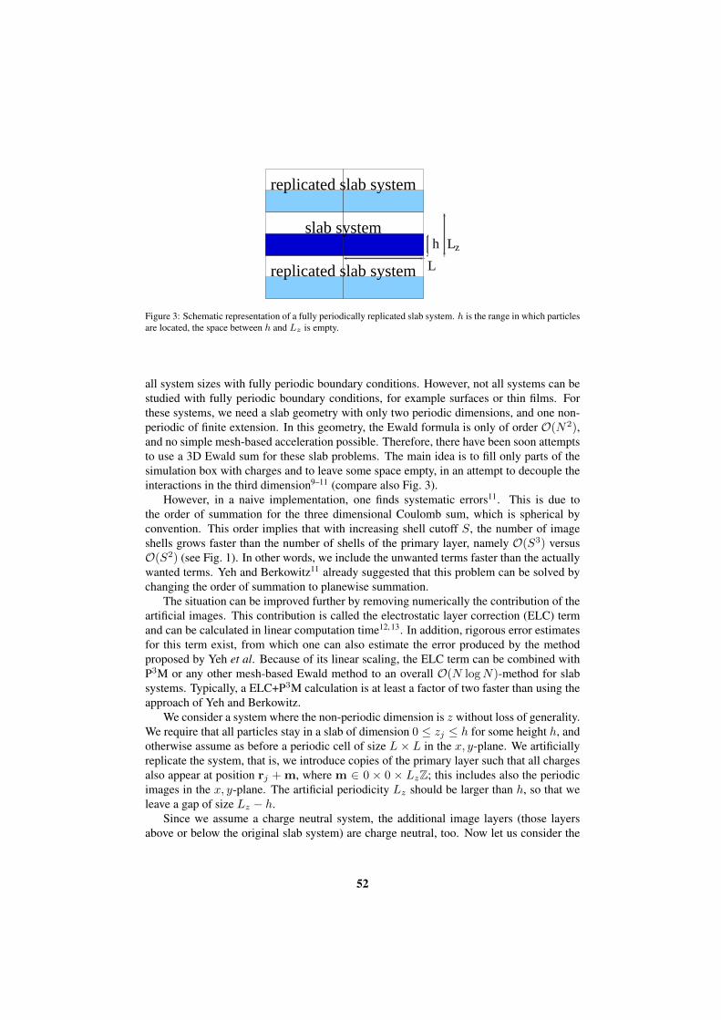
replicated slab system
slab system h
replicated slab system
L
L
z
Figure 3: Schematic representation of a fully periodically replicated slab system. h is the range in which particlesare located, the space between h and Lz is empty.
all system sizes with fully periodic boundary conditions. However, not all systems can bestudied with fully periodic boundary conditions, for example surfaces or thin films. Forthese systems, we need a slab geometry with only two periodic dimensions, and one non-periodic of finite extension. In this geometry, the Ewald formula is only of order O(N2),and no simple mesh-based acceleration possible. Therefore, there have been soon attemptsto use a 3D Ewald sum for these slab problems. The main idea is to fill only parts of thesimulation box with charges and to leave some space empty, in an attempt to decouple theinteractions in the third dimension9–11 (compare also Fig. 3).
However, in a naive implementation, one finds systematic errors11. This is due tothe order of summation for the three dimensional Coulomb sum, which is spherical byconvention. This order implies that with increasing shell cutoff S, the number of imageshells grows faster than the number of shells of the primary layer, namely O(S3) versusO(S2) (see Fig. 1). In other words, we include the unwanted terms faster than the actuallywanted terms. Yeh and Berkowitz11 already suggested that this problem can be solved bychanging the order of summation to planewise summation.
The situation can be improved further by removing numerically the contribution of theartificial images. This contribution is called the electrostatic layer correction (ELC) termand can be calculated in linear computation time12, 13. In addition, rigorous error estimatesfor this term exist, from which one can also estimate the error produced by the methodproposed by Yeh et al. Because of its linear scaling, the ELC term can be combined withP3M or any other mesh-based Ewald method to an overall O(N logN)-method for slabsystems. Typically, a ELC+P3M calculation is at least a factor of two faster than using theapproach of Yeh and Berkowitz.
We consider a system where the non-periodic dimension is z without loss of generality.We require that all particles stay in a slab of dimension 0 ≤ zj ≤ h for some height h, andotherwise assume as before a periodic cell of size L × L in the x, y-plane. We artificiallyreplicate the system, that is, we introduce copies of the primary layer such that all chargesalso appear at position rj + m, where m ∈ 0 × 0 × LzZ; this includes also the periodicimages in the x, y-plane. The artificial periodicity Lz should be larger than h, so that weleave a gap of size Lz − h.
Since we assume a charge neutral system, the additional image layers (those layersabove or below the original slab system) are charge neutral, too. Now let us consider the
52

mth image layer, which has an offset of mLz to the original layer. If Lz is large enough,each particle in themth layer and its replicas in the x, y-plane can be viewed as constitutinga homogeneous charged sheet of charge density σj =
qjL2 . The potential of such a charged
sheet at distance z is 2πσj |z|; the interaction of a pair of image layers located at zj±mLz ,with a charge qi in the primary layer is therefore approximately
2πqi
N∑j=1
σj(|zj − zi +mLz|+ |zj − zi −mLz|) = 4πqi nLz
N∑j=1
σj = 0. (38)
The only errors occurring are those coming from the approximation of assuming homo-geneously charged, infinite sheets instead of discrete charges, which should reduce withincreasing distance |m|Lz from the central layer. Naturally, this argument only holds whenusing planewise summation. Yeh and Berkowitz stated that a gap size of at least h is nor-mally sufficient to obtain an moderately accurate result. However, no theoretical estimatesexist for the error introduced by the image layers, which could justify this statement; wewill see that it is in fact not true. Therefore one might be forced to use even larger gapsto assure that no artifacts are produced by the image layers. One simple deducible artifactis that the pairwise error will be position dependant. Particles in the middle of the slabwill see no effect of the image layers due to symmetry, and particles near the surface willencounter for the same reason the largest errors, which is definitely an unwanted featurefor studying surface effects.
The ELC term is the energy contribution of the artificially introduced image layers, thatis
Ulc = −1
2
∑m>0
∑m∈Z2×±mLz/L
N∑i,j=1
qiqj|rij −mL| , (39)
Since we assume that the image layers all are separated from the main layer by at least thegap size Lz − h, we can use a convergence factor approach to calculate the interaction ofthe primary layer with the image layer m. More precisely, we use a screened Coulombpotential e−βr
r in the limit of infinite screening length β−1. The screened potential canbe conveniently Fourier transformed along each of the two periodic coordinates, and oneobtains35, 36, 12
Ulc(m) = −1
2
N∑i,j=1
qiqj2π
L2
∑k∈ 2π
L Z2
k2>0
e−|k||zij−mLz|
|k| ei(kxxij+kyyij) − 2π
L2|zij −mLz|.
(40)The sum over m to obtain Ulc can be performed analytically by a geometric series. Theterms 2π
L2 |zij −mLz| are exactly the homogeneous sheet potential, which we have seen to
53
cancel out for charge neutral systems (see Eqn. (38)). We obtain the ELC term
Ulc =π
L2
∑k∈ 2π
L Z2
k2>0
N∑i,j=1
qiqje|k|zij + e−|k|zij
fpq(efpqLz − 1)ei(kxxij + kyyij)
=π
L2
∑k∈ 2π
L Z2
k2>0
N∑i=1
qie|k|ziei(kxxi + kyyi)
fpq(e|k|Lz − 1)
N∑j=1
qje−|k|zje−i(kxxj − kyyj)
+π
L2
∑k∈ 2π
L Z2
k2>0
N∑i=1
qie−|k|ziei(kxxi + kyyi)
|k|(e|k|Lz − 1)
N∑j=1
qje|k|zje−i(kxxj − kyyj).
(41)
The forces can be obtained by simple differentiation since the sums are absolutely conver-gent. Although Eqn.(41) has a much better convergence than the original form in Eqn.(39),its main advantage is a linear computation time with respect to the number of particles N ,since the two sums over N can be evaluated independently. Just as for the classical Ewaldmethod, parallelization is trivial, since we only need to calculate simple sums over allcompute nodes, for which efficient reduce operations exist in the MPI standard.
To complete the calculation, one of course still needs the forces and energies of thefully periodic system, for example calculated by the P3M method. However, it is vital touse the correct summation order, that is, dipole term. Since we performed the summationover the image layers explicitely layer by layer, also the 3D summation has to be performedin the same order. This means, that one has to use the dipole term according to Eqn. (10),just as in the method proposed by Yeh and Berkowitz.
Similar to P3M it is possible to consider non-neutral systems37. To this aim, one firstneutralizes the system using a homogeneous background for the calculation using the 3Dmethod, e.g. P3M . This homogeneous background gives rise to an unwanted force thatdrives the particles towards the boundaries of the system. However, one can calculate thisforce analytically, and subtract it again. Note that the background also contributes to thedipole term for slabwise summation. It should now read:
U (d) =2π
V
[ N∑i=1
qi
(zi −
Lz2
)]2
, (42)
where the shift accounts for the neutralizing background, which in the slab system is ahomogeneous charge in the range from 0 toLz . For an Ewald-type method, the neutralizingbackground term U (n) according to Eqn. (11) is required in addition. The interactionenergy of the background with the slab system and itself is finally
U (b) =2π
V
N∑i=1
qi
N∑j=1
qjzj (Lz − zj) −1
3
( N∑i=1
qi
)2 , (43)
which we need to subtract together with the ELC correction.
54

1e-05
0.0001
0.001
0.01
0.1
1
0 1 2 3 4 5 6 7 8 9
∆Fz
z
1e-05
0.0001
0.001
0.01
0.1
1
0 1 2 3 4 5
∆Fz
z
Figure 4: Absolute RMS force error ∆Fz as a function of the particle’s z–coordinate for a homogeneous randomsystem of 1000 particles in a box of size 10 × 10 × h with a system height h = 9 (left graph) and 5 (rightgraph). The curves are from top to bottom: results for cutoff R = 0, i. e. the Yeh and Berkowitz approach, forR = 1 and R = 1.8 in the left graph with h = 9. In the right graph with h = 5, we also use R = 0, but thenR = 0.1 and R = 0.3. These cutoffs correspond to similar boundary errors for both heights, showing that oneneeds larger cutoffs with decreasing gap size. We used P3M as the underlying 3D method, tuned for a RMS forceerror of 10−4. The overall accuracy is limited by this P3M error, the accuracy of ELC in the center of the systemis much better.
4.1 Error estimates
Like before, we want to estimate the error that we introduce by the necessary truncationof the Fourier sum. While for the standard Ewald sum, this was only used to tune thealgorithm, the error estimates for ELC can also be used to estimate the error that oneintroduces by not taking into account the ELC term at all, that is, using the slab-wisemethod of Yeh and Berkowitz11. Our error estimates can be used to determine “a priori” thenecessary gap size to reach a preset precision without calculating the ELC term. Thereforewe also have to deal with small cutoffs, especially the case when no terms ofElc are added.
We assume that the Fourier sum is truncated at a cutoff of kmax, that is, the summationis performed only over all (p, q) ∈ (2πLZ)2, where 0 < p2 + q2 ≤ k2
max. An upper boundfor the absolute value of the summands is
2π
L2
∣∣∣∣ cosh(|k|zij)|k|(e|k|Lz − 1)
eikxxijeikyyij
∣∣∣∣ ≤ 2π
L2e−2π|k|Lz cosh(|k|zij)
|k|(1− e−|k|Lz ) . (44)
The sum over all these upperbounds can then be performed by an careful approximation ofthe sum by an integral, which will give an upper bound for the algorithm dependent factorχ of Eqn. (22). From that, we obtain a limit for the RMS force error:
∆F ≤∑q2i
2√N(ekmaxLz − 1)
[(kmax +
4
L+
1
Lz − h
)ekmaxh
(Lz − h)+
(kmax +
4
L+
1
Lz + h
)e−kmaxh
(Lz + h)
] (45)
≈∑q2i kmax
2√N(Lz − h)
e−kmax(Lz−h), (46)
55

lz εm
εt
z
x
εb
q
q
q
q
q∆t
∆t
∆b
∆b
∆b∆t
Figure 5: A schematic view of image charges. The dielectric interfaces are characterized by the εt−εm and εm−εb boundaries, which give rise to an infinite number of image charges along the z-direction due to polarizationand multiple reflection under two parallel dielectrics. In the x, y-direction the image charges due to periodicboundaries are shown. The dotted lines are only provided to visualize the positioning of the image charges.
where the latter simplification is only valid for large kmax. The total error of the combina-tion of ELC and any 3D method can be obtained again by summing up the error contribu-tions according to Eqn. (23).
Our error estimates show that the error drops exponential both with kmax and Lz . Thismeans that it is easy to achieve increase the accuracy with our layer correction formula,either by increasing the k-space cutoff or the gap size. An upper bound for the errorproduced by the method of Yeh and Berkowitz can be obtained by inserting kmax = 2π 1
L .In this case, the error formula shows that the error decays with the ratio kmax(Lz − h) ∼(Lz − h)/L and not Lz/h, as was claimed by Yeh and Berkowitzb.
Note that Eqn. (44) shows that the error in the potential or the force for a single particlewill be largest if it is located near the gap, since there |zij |will be maximal. This effect willincrease with increasing R, therefore, it is important to tune ELC (and with that, also themethod of Yeh and Berkowitz) to errors small enough to be negligible even at the systemboundaries. Just measuring the overall RMS force error might be misleading, especially,since for thin films or surfaces, mostly the particles at the surfaces are of interest. This isdemonstrated in Fig 4.
If one assumes an mesh-based Ewald method to be used for the 3D periodic system,one can estimate the optimal Lz as follows. The computation time of the mesh method isproportional to V = L2Lz . For ELC, kmax is proportional to 1/(Lz − h), therefore thecomputation time spent with ELC is proportional to L2/(Lz − h)2. The total computationtime is therefore minimized by a constant gap size independent of the box dimensions.
4.2 Varying dielectric constants
In the three dimensional Ewald sum, the dielectric constant at infinity, ε′, plays an impor-tant role through the dipole term (9). This is of physical origin, as can be seen from thefact that the dipole term is not algorithm dependent. For systems with only two periodicdimensions, the dielectric constant at infinity does not play a role; however, it may be nec-essary to include dielectric contrasts in the non-periodic coordinate. For example, a thin
bIn fact, already the extreme case of h = 0 immediately shows that this cannot be true, as a conventional methodfor three dimensional periodicity will not deliver exact results for a purely planar system.
56

water film in vacuum has a dielectric constant of ε ≈ 80, while the surrounding vacuumhas ε = 1. The dielectric contrasts at the film boundaries give rise to an infinite series ofimage charges, which can be taken into account by the ELC method37.
We assume that the charges are all contained in a medium of height Lz and a dielectricconstant εm, which is sandwiched from above by a medium of dielectric constant εt andfrom below by a medium of dielectric constant εb (compare Fig. 5 left). We define thedielectric contrasts
∆b =εm − εbεm + εb
, and ∆t =εm − εtεm + εt
, (47)
and the double reflection factor ∆ = ∆b∆t. Then the potential of each charge includingits polarization images is represented by the following four series of charges:
• charges qi∆n at positions zi − 2Lzn, n ≥ 0 (this series also includes the real charge)
• charges qi∆b∆n at positions −zi − 2Lzn, n ≥ 0
• charges qi∆n at positions zi + 2Lzn, n ≥ 1
• charges qi∆t∆n at positions −zi + 2Lz(n+ 1), n ≥ 0.
What we are interested in is the electrostatic energy, that is, the energy of the real chargesdue to the potential generated by (a) the real particles, (b) the image charges due to thedielectric boundaries and (c) the periodic images of both.
Even though the task looks daunting, the solution turns out to be simple. Basically, thesum of the potential generated by each of the charge series is again a geometric series inthe image layer count, which once more can be calculated by Eqn. (40) and summed upanalytically. One just has to be careful with the images that are close to the primary layer;here, a direct summation, that is, the application of for example ELC+P3M is required. Forfurther details, see Ref. 37.
5 Dipolar Ewald Summation in 3D
In the previous section we treated methods to deal with the Coulomb interaction, or moregenerally, interactions which vary with 1/r. In this section, we turn towards another elec-trostatic interaction, namely the dipolar interaction. For (fully) periodic geometries againthe Ewald method can be used, with the same computation time scale as for the Coulombinteraction, that is at best O(N3/2), if the cutoff is optimally varied with the splitting pa-rameter5. For MC simulations, knowing the energy formulas is sufficient, whereas for MDsimulations, we need to know forces and torques. In this section we show how the Ewaldsum can be used also for dipolar interactions, and give a reliable error estimate for theforces and the torques15.
Consider a system of N particles with a point-dipole µi at their center position ri ina cubic simulation box of length L. If periodic boundary conditions are applied, the totalelectrostatic energy of the box is given by
U =1
2
∑m∈Z3
N∑′
i,j=1
µi · µj
|rij + mL|3 −3[µi · (rij + mL)][µj · (rij + mL)]
|rij + mL|5, (48)
57

where the prime indicates that the i = j term must be omitted for m = 0. The slowlydecaying long range part of the dipolar potential makes the straightforward summation ofEqn. (48) too time consuming. The Ewald trick splits the problem again into two rapidlyconvergent parts, one in real space and one in reciprocal space. The details of the methodare discussed in Refs.1, 5, 19, 3, here we only give the final expressions. The energy is
U = U (r) + U (k) + U (s) + U (d), (49)
where the real-space U (r), the k-space (reciprocal space) U (k), the self U (s) and the dipole(surface) U (d) contributions are respectively given by:
U (r) =1
2
∑m∈Z3
N∑′
i,j=1
(µi · µj)B(|rij + mL|)
− [µi · (rij + mL)][µj · (rij + mL)]C(|rij + mL|),
(50)
U (k) =1
2L3
∑k6=0
4π
k2e−(πk/αL)2
N∑i,j=1
(µi · k)(µj · k)e2πik·rij/L, (51)
U (s) = − 2α3
3√π
N∑i=1
µ2i , (52)
U (d) =2π
(2ε′ + 1)L3
N∑i,j=1
µi · µj . (53)
The k-sum is again over reciprocal vectors k ∈ 2πL Z3, the sums over i and j are for the
particles in the central box and
B(r) = [erfc(αr) + (2αr/√π) exp(−α2r2)]/r3, (54)
C(r) = [3 erfc(αr) + (2αr/√π)(3 + 2α2r2) exp(−α2r2)]/r5. (55)
The inverse length α is the splitting parameter of the Ewald summation which shouldbe chosen so as to optimize the performance. The form Eqn. (53) for the surface termagain assumes spherical summation and that the medium outside the growing sphere is anuniform dielectric with dielectric constant ε′.
In practical calculations, the infinite sums in Eqns. (50) and (51) are truncated by onlytaking into account distances which are smaller than some real space cutoff rmax and wavevectors with a modulus smaller than some reciprocal space cutoff kmax. If rmax ≤ L/2,the sum in real space [Eqn. (50)] reduces to the normal minimum image convention. Thedouble sum over particles in U (k) can be replaced by a product of two single sums whichis more suitable for numerical calculations.
The force Fi acting on particle i is obtained by differentiating the non-constant contri-butions to the potential energy U with respect to ri, i.e.,
Fi = − ∂
∂riU = F
(r)i + F
(k)i , (56)
58

with the real-space and k-space contributions given by:
F(r)i =
∑m∈Z3
N∑′
j=1
[(µi · µj)rmij + µi(µj · rmij ) + (µi · rmij )µj
]C(rmij )
− (µi · rmij )(µj · rmij )D(rmij ) rmij
,
(57)
F(k)i =
2π
L4
N∑j=1
∑k6=0
4πk
k2
[(µi · k)(µj · k) exp[−(πk/αL)2]
· sin(2πk · rij/L)],
(58)
where rmij = rij + mL and
D(r) = [15 erfc(αr) + (2αr/√π)(15 + 10α2r2 + 4α4r4) exp(−α2r2)]/r7. (59)
Since the self and surface energy terms [Eqns. (52), (53)] are independent of the particlepositions, they have no contributions to the force, unlike the Ewald sum for Coulombsystems where the surface term contributes. The torque τ i acting on particle i is related tothe electrostatic field Ei at the location of this particle via
τ i = µi ×Ei = τ(r)i + τ
(k)i + τ
(d)i , (60)
with
Ei = − ∂
∂µiU, (61)
and thus
τ(r)i =−
∑m∈Z3
N∑′
j=1
(µi × µj)B(rmij )− (µi × rmij )(µj · rmij )C(rmij )
, (62)
τ(k)i =− 1
L3
N∑j=1
∑k∈Z3,k 6=0
4π
k2(µi × k)(µj · k)e−(πk/αL)2e2πik·rij/L, (63)
τ(d)i =− 4π
(2ε′ + 1)L3
N∑j=1
µi × µj . (64)
5.1 Error Formulas
We now give estimates for the RMS error caused by cutting off the Ewald summation inreal-space and k-space for the forces and the torques. There are no errors involved in theself and surface contributions [Eqns. (52), (53) and (64)], because no cutoff operations areapplied to them. As can be shown similarly to the way as it was presented in Sec. 2.1, theRMS error for the force can be cast in the following form
∆F ≈ χM2
√N
with M2 :=
N∑j=1
µ2j . (65)
59

After some lengthy calculation one obtains for the algorithmic contribution from thereal space15
χ(r)2 ≈ L−3r−9maxα
−4(13
6C2c +
2
15D2c −
13
15CcDc) exp(−2α2r2
max), (66)
where the terms Cc and Dc are given by
Cc = 4α4r4max + 6α2r2
max + 3, (67)
Dc = 8α6r6max + 20α4r4
max + 30α2r2max + 15. (68)
The resulting RMS expectation of the real-space cutoff error in the forces is thus
∆F (r) ≈M2(L3α4r9maxN)−1/2(
13
6C2c +
2
15D2c −
13
15CcDc)
1/2 exp(−α2r2max) (69)
and in the torques
∆τ (r) ≈M2(L3α4r7maxN)−1/2[
1
2B2c +
1
5C2c ]1/2 exp(−α2r2
max). (70)
Eqns. (69) and (70) both contain the exponential exp(−α2r2max). For sufficiently low
errors, αrmax has to be larger than one, for example αrmax ≈ π for an error ofexp(−π2) ≈ 5× 10⁻⁵. If only the highest powers of αrmax are retained, the estimates ofdrastically simplify to
∆F (r) ≈ 8M2α4(2r3max/15NL3)1/2 exp(−α2r2
max), (71)
∆τ (r) ≈ 4M2α2(rmax/5NL3)1/2 exp(−α2r2
max), (72)
The advantage of these simplified formulas is that they reflect the dependence of the RMSerrors on α and rmax more directly and thus could be used more easily in determining theoptimal values of these parameters.
In deriving the estimates of the reciprocal-space (k-space) cutoff errors, we assume thatthe radial distribution function of the particles is approximately unity at all distances. Thenone finds the RMS expectation of the k-space cutoff error in the forces as15
∆F (k) ≈ 8πM2L−3α(2πk3max/15N)1/2 exp[−(πkmax/αL)2], (73)
and in the torques
∆τ (k) ≈ 4M2L−2α(πkmax/5N)1/2 exp[−(πkmax/αL)2]. (74)
The total error can be obtained again by taking into account the real and k-space errorsaccording to Eqn. (23).
5.2 Optimization of Parameters
In this section, we discuss the use of the analytical formulas derived in Sec. III to determinethe optimal values of α, rmax and kmax by which the required accuracy could be satisfiedand the computation time is minimized. The detailed discussions on this subject can also befound in Refs.5, 27. First, we note that the same argumentation as for the Coulombic Ewaldsum holds, namely that the computation time is T = O(Nα−3) + O(N2α3), which isminimized by α ∼ N−1/6. Therefore, the optimal computation time of the dipolar Ewaldsum is as well O(N3/2).
60

1000 10000 1e+05 1e+06N
10
α (1
/L)
δ = 10−2
δ = 10−3
δ = 10−4
δ = 10−5
(a)
31000 10000 1e+05 1e+06
N
1
10
100
k c
δ = 10−2
δ = 10−3
δ = 10−4
δ = 10−5
(b)
1000 10000 1e+05 1e+06N
1
10
r c
δ = 10−2
δ = 10−3
δ = 10−4
δ = 10−5
(c)
1000 10000 1e+05 1e+06N
0.0001
0.001
0.01
0.1t/N
δ = 10−2
δ = 10−3
δ = 10−4
δ = 10−5
(d)
Figure 6: Optimal values of the parameters α (a), kmax (b) and rmax (c) as well as the corresponding minimizedcomputation time T /N (d) as a function of the number of particles.
The numerical investigation of the functional dependence of the optimal parameters onN and δ are performed as follows. For each given N and δ, we at first choose differentvalues for rmax within the inequality rmax ≤ L/2. For each rmax the parameters α andkmax are calculated by solving Eqns. (71)) and (73). Now, one can perform a trial com-putation to measure the required computer time for each rmax, and by this figure out theoptimal value of rmax which gives the minimum computation time. In our calculations thesize of the simulation cell is fixed to a dimensionless length of L = 10. The range of ac-curacy requirement and number of particles are chosen to be δ = 10−2 to 10−5 measuringin P2/L4 and N = 103 to N = 106 which should cover most of the applications. Theparticles are supposed to have an uniform dipole moment of P . The results for the optimalvalues of the parameters and the corresponding computation time per particle are shownin Fig. 6 (a-d), respectively. It can be clearly seen that the functional dependence of theparameters and the overall computation time on N are just as discussed above. Fig. 6(c)shows that when a high accuracy is required for a system with a small number of particles,the predicted real-space cutoff is larger than half of the box length and rmax = L/2 mustbe used, which prohibits the use of the minimum image convention. The optimal α valueshardly depend on the accuracies. Note that unlike in the discussion above, we assume a
61
constant volume and thus the optimal α ∼ N1/6 instead of N−1/6, as can be easily seen;the overall optimal computation time at constant volume is still O(N3/2).
Finally we should remark that besides the standard Ewald method, dipolar variants ofbasically all Coulomb solvers are possible; a dipolar SPME has been described in Ref. 38,a dipolar P3M with optimal influence function and known error estimates in Ref. 39, andthe ELC term was derived for dipolar systems in Ref. 40.
6 Concluding Remarks
We have given a review of Fourier transform-based methods to compute the electrostaticinteraction. We have shown that this oldest family of Coulomb solvers is very versatileand can be applied to systems with any combination of periodic boundary conditions andalso to dipolar interactions. We tried to give reasons why one should worry about errors,and gave error estimates for all presented algorithms. We also described how these errorestimates can be used to tune the algorithms to perform optimally for speed and accuracy.
References
1. P. P. Ewald, Die Berechnung optischer und elektrostatischer Gitterpotentiale, Ann.Phys., 369, no. 3, 253–287, 1921.
2. D. M. Heyes, Electrostatic potentials and fields in infinite point charge lattices,J. Chem. Phys., 74, no. 3, 1924–1929, 1981.
3. S. W. de Leeuw, J. W. Perram, and E. R. Smith, Simulation of Electrostatic Systemsin Periodic Boundary Conditions. I. Lattice Sums and Dielectric Constants, Proc. R.Soc. Lond., A, 373, no. 1752, 27–56, 1980.
4. S. W. de Leeuw, J. W. Perram, and E. R. Smith, Simulation of Electrostatic Systemsin Periodic Boundary Conditions. II. Equivalence of Boundary Conditions, Proc. R.Soc. Lond., A, 373, no. 1752, 57–66, 1980.
5. John W. Perram, Henrik G. Petersen, and Simon W. de Leeuw, An algorithm forthe simulation of condensed matter which grows as the 3/2 power of the number ofparticles, Mol. Phys., 65, no. 4, 875–893, 1988.
6. M. Deserno and C. Holm, How to mesh up Ewald sums. I. A theoretical and numericalcomparison of various particle mesh routines, J. Chem. Phys., 109, 7678, 1998.
7. M. Deserno and C. Holm, How to mesh up Ewald sums. II. An accurate error estimatefor the Particle-Particle-Particle-Mesh algorithm, J. Chem. Phys., 109, 7694, 1998.
8. Albert H. Widmann and David B. Adolf, A comparison of Ewald summation tech-niques for planar surfaces, Comput. Phys. Commun., 107, 167–186, 1997.
9. J. C. Shelley and G. N. Patey, Boundary condition effects in simulations of waterconfined between planar walls, Mol. Phys., 88, 385, 1996.
10. E. Spohr, Effect of electrostatic boundary conditions and system size on the interfacialproperties of water and equeous solutions, J. Chem. Phys., 107, 6342, 1997.
11. In-Chul Yeh and Max L. Berkowitz, Ewald summation for systems with slab geome-try, J. Chem. Phys., 111, no. 7, 3155–3162, 1999.
12. A. Arnold, J. de Joannis, and C. Holm, Electrostatics in Periodic Slab Geometries I,J. Chem. Phys., 117, 2496–2502, 2002.
62
13. A. Arnold, J. de Joannis, and C. Holm, Electrostatics in Periodic Slab Geometries II,J. Chem. Phys., 117, 2503–2512, 2002.
14. R. E. Rosensweig, Ferrohydrodynamics, Cambridge Univ. Press, Cambridge, 1985.15. Z. W. Wang and C. Holm, Estimate of the Cutoff Errors in the Ewald Summation for
Dipolar Systems, J. Chem. Phys., 115, 6277–6798, 2001.16. C. Holm, “Efficient methods for long range interactions in periodic geometries plus
one application”, in: Computational Soft Matter: From Synthetic Polymers to Pro-teins, N. Attig, K. Binder, H. Grubmuller, and K. Kremer, (Eds.), vol. 23 of NICseries. Research Centre Julich, 2004.
17. A. Arnold and C. Holm, “Efficient methods to compute long range interactions forsoft matter systems”, in: Advanced Computer Simulation Approaches for Soft MatterSciences II, C. Holm and K. Kremer, (Eds.), vol. II of Advances in Polymer Sciences,pp. 59–109. Springer, Berlin, 2005.
18. D. Frenkel, Colloidal systems: Playing Tricks with Designer ”Atoms”, Science, 296,65, 2002.
19. Mike P. Allen and Dominik J. Tildesley, Computer Simulation of Liquids, OxfordScience Publications. Clarendon Press, Oxford, 1 edition, 1987.
20. Jean-Michel Caillol, Comments on the numerical simulation of electrolytes in peri-odic boundary conditions, J. Chem. Phys., 101, no. 7, 6080–6090, 1994.
21. Stefan Boresch and Othmar Steinhauser, Presumed Versus Real Artifacts of the EwaldSummation Technique: The Importance of Dielectric Boundary Conditions, Ber. Bun-senges. Phys. Chem., 101, no. 7, 1019–29, 1997.
22. H. J. C. Berendsen, in: Computer Simulation of Biomolecular Systems, Wilfred F. vanGunsteren, P. K. Weiner, and A. J. Wilkinson, (Eds.), vol. 2, pp. 161–81, ESCOM,The Netherlands, 1993.
23. Philippe H. Huenenberger, Optimal charger-shaping functions for the particle-particle-particle-mesh (P3M) method for computing electrostatic interactions inmolecular simulations, J. Chem. Phys., 113, no. 23, 10464–10476, 2000.
24. E. R. Smith, Electrostatic potentials for thin layers, Mol. Phys., 65, 1089–1104, 1988.25. Gerhard Hummer, Lawrence R. Pratt, and Angle E. Garcıa, Molecular Theories and
Simulation of Ions and Polar Molecules in Water, J. Phys. Chem. A, 102, no. 41,7885–97, 1998.
26. Jiri Kolafa and John W. Perram, Cutoff errors in the Ewald summation formulae forpoint charge systems, Mol. Simul., 9, no. 5, 351–368, 1992.
27. Henrik G. Petersen, Accuracy and efficiency of the particle mesh Ewald method,J. Chem. Phys., 103, no. 9, 3668–3679, 1995.
28. R. W. Hockney and J. W. Eastwood, Computer Simulation Using Particles, IOP, Lon-don, 1988.
29. T. Darden, D. York, and L. Pedersen, Particle Mesh Ewald: An N log(N) method forEwald sums in large systems, J. Chem. Phys., 98, 10089–10092, 1993.
30. U. Essmann, L. Perera, M. L. Berkowitz, T. Darden, H. Lee, and L. Pedersen, Asmooth Particle Mesh Ewald method, J. Chem. Phys., 103, 8577, 1995.
31. I. J. Schoenberg, Cardinal Spline Interpolation, Society for Industrial and AppliedMathematics, Philadelphia, 1973.
32. David S. Cerutti, Robert E. Duke, Thomas A. Darden, and Terry P. Lybrand, Stag-gered Mesh Ewald: An Extension of the Smooth Particle-Mesh Ewald Method AddingGreat Versatility, J. Chem. Theory Comput., 5, no. 9, 2322–2338, 2009.
63

33. A. Neelov and C. Holm, Interlaced P3M algorithm with analytical and ik-differentiation, J. Chem. Phys., 132, no. 23, 234103, 2010.
34. Matteo Frigo and Steven G. Johnson, The Design and Implementation of FFTW3,Proceedings of the IEEE, 93, no. 2, 216–231, 2005, Special issue on “Program Gen-eration, Optimization, and Platform Adaptation”.
35. A. Arnold and C. Holm, MMM2D: A fast and accurate summation method for elec-trostatic interactions in 2D slab geometries, Comput. Phys. Commun., 148, no. 3,327–348, 2002.
36. A. Arnold and C. Holm, A novel method for calculating electrostatic interactions in2D periodic slab geometries, Chem. Phys. Lett., 354, 324–330, 2002.
37. Sandeep Tyagi, Axel Arnold, and Christian Holm, Electrostatic layer correction withimage charges: A linear scaling method to treat slab 2D + h systems with dielectricinterfaces, J. Chem. Phys., 129, no. 20, 204102, 2008.
38. Abdulnour Toukmaji, Celeste Sagui, John Board, and Tom Darden, Efficientparticle-mesh Ewald based approach to fixed and induced dipolar interactions,J. Chem. Phys., 113, no. 24, 10913–10927, 2000.
39. Juan J. Cerda, V. Ballenegger, O. Lenz, and Ch. Holm, P3M algorithm for dipolarinteractions., J. Chem. Phys., 129, 234104, 2008.
40. A. Brodka, Ewald summation method with electrostatic layer correction for interac-tions of point dipoles in slab geometry, Chem. Phys. Lett., 400, no. 1-3, 62–67,2004.
64
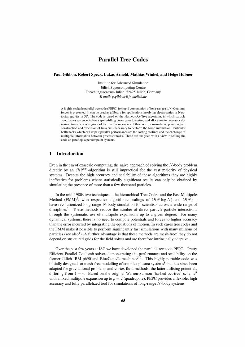
Parallel Tree Codes
Paul Gibbon, Robert Speck, Lukas Arnold, Mathias Winkel, and Helge Hubner
Institute for Advanced SimulationJulich Supercomputing Centre
Forschungszentrum Julich, 52425 Julich, GermanyE-mail: [email protected]
A highly scalable parallel tree code (PEPC) for rapid computation of long-range (1/r) Coulombforces is presented. It can be used as a library for applications involving electrostatics or New-tonian gravity in 3D. The code is based on the Hashed-Oct-Tree algorithm, in which particlecoordinates are encoded on a space-filling curve prior to sorting and allocation to processor do-mains. An overview is given of the main components of this code: domain decomposition, treeconstruction and execution of traversals necessary to perform the force summation. Particularbottlenecks which can impair parallel performance are the sorting routines and the exchange ofmultipole information between processor tasks. These are analysed with a view to scaling thecode on petaflop supercomputer systems.
1 Introduction
Even in the era of exascale computing, the naive approach of solving the N -body problemdirectly by an O(N2)-algorithm is still impractical for the vast majority of physicalsystems. Despite the high accuracy and scalability of these algorithms they are highlyineffective for problems where statistically significant results can only be obtained bysimulating the presence of more than a few thousand particles.
In the mid-1980s two techniques – the hierarchical Tree Code1 and the Fast MultipoleMethod (FMM)2, with respective algorithmic scalings of O(N logN) and O(N) –have revolutionized long-range N -body simulation for scientists across a wide range ofdisciplines3. These methods reduce the number of direct particle-particle interactionsthrough the systematic use of multipole expansions up to a given degree. For manydynamical systems, there is no need to compute potentials and forces to higher accuracythan the error incurred by integrating the equations of motion. In such cases tree codes andthe FMM make it possible to perform significantly fast simulations with many millions ofparticles (see also4). A further advantage is that these methods are mesh-free: they do notdepend on structured grids for the field solver and are therefore intrinsically adaptive.
Over the past few years at JSC we have developed the parallel tree code PEPC – PrettyEfficient Parallel Coulomb-solver, demonstrating the performance and scalability on theformer Julich IBM p690 and BlueGene/L machines5–7. This highly portable code wasinitially designed for mesh-free modelling of complex plasma systems8, but has since beenadapted for gravitational problems and vortex fluid methods, the latter utilising potentialsdiffering from 1 − r. Based on the original Warren-Salmon ’hashed oct-tree’ scheme9
with a fixed multipole expansion up to p = 2 (quadrupole), PEPC provides a flexible, highaccuracy and fully parallelized tool for simulations of long-range N -body systems.
65

We begin this overview with a general outline of the parallel tree code PEPC, and thenproceed to describe the main steps involved to compute the potentials and/or forces on a setof particles: the distribution and decomposition of the particles among processor tasks, thetree construction and multipole definitions, the determination of interaction lists and forcesummation, including a recent extension to periodic systems. In Section 3 we presentperformance analyses of the code on the Julich supercomputers Jugene and Juropa.
2 Parallel Tree Codes: the Basics
Algorithmically speaking, an electrostatic tree code is no different to the various New-tonian gravity N -body solvers used in astrophysics, which are nearly all based on someform of the Barnes-Hut hierarchical tree algorithm1. Briefly summarized: the electrostaticforce-sum on each particle is computed by systematically replacing more distant chargesby multipole expansions of charge groups, thus reducing the standard O(N2) direct sumto an O(N logN) complexity at the price of a small, controllable error3. For many appli-cations – for example in plasma or astrophysics – there is little to be gained in computingpotentials and forces to higher accuracy than the error incurred by time-integration, whichcan be anywhere between 10−4 for a high-order Runge-Kutta scheme, to around 1% forthe simple 2nd-order Leap-Frog method.
for all iteration steps do
domain decomposition:convert local particle coordinates to keysperform global key-sort
build tree:construct local nodesdefine global branchesfill in top-level nodescompute multipole properties
define particle chunksfor each chunk do
perform tree traversalperform force summation
end for
end for
Figure 1: Outline of parallel tree code: for dynamical systems, the tree and interaction lists are built afresh eachtimestep.
The price to be paid for the speed-up in the force sum is a considerable increase in pro-gramming complexity. First, the hierarchical data structure necessary to navigate around
66

the tree introduces an unavoidable bookkeeping overhead. Second, accessing multipoleinformation lying on remote processors results in additional communication, which if notcarefully implemented, can result in poor parallel efficiency. These issues notwithstanding,each step in the scheme illustrated in Fig.1 can be implemented in parallel with a scalinglike N/P or N logN/P .
2.1 Domain decomposition
At first sight, the hierarchical data structure required in a tree code to manage the multi-pole information would seem to preclude parallelism altogether. In fact, several schemesfor parallel tree codes have been proposed and implemented, including virtual shared-memory versions10, and distributed memory schemes using geometrical domain decom-position methods11, 12. The scheme adopted here follows the one devised by Salmon andWarren13, 9, who practically reinvented the BH algorithm by scrapping memory pointers forbookkeeping in favour of a set of universal binary keys to represent particle and tree-nodecoordinates alike.
The basic idea is to convert the coordinate triple of each particle into a single, unique64-bit integer key. The keys do not replace the coordinates, but as we shall see, provide anatural and rapid means of sorting the particles and building up the tree structure aroundthem. Given its key and owner, locating any node in the tree is reduced to an O(1) opera-tion.
In the present code, PEPC, the keys are constructed from the binary interleave opera-tion:
k = p+
7∑j=0
8j [4 × bit(iz, j, 1) + 2 × bit(iy, j, 1) + bit(ix, j, 1)] (1)
The function bit(a,j,1) selects 1 bit of the integer a starting from bit position j. Thenormalized integer coordinates are computed from:
ix = x/s
iy = y/s
iz = z/s (2)
where
s = L/2nlevels
and L is the simulation box length; nlevels the maximum refinement level. The latterobviously depends on the machine precision, and for a 64-bit machine, we can have 21 bitsper coordinate (or nlevels=20) plus a place-holder bit:
p = 263.
The place-holder bit is necessary to distinguish genuine particles on the lowest levelsof the tree from higher level nodes of the internal tree structure. Mapping the coordinatesto keys in this manner yields a space-filling curve, in this case following a pattern known asMorton- or Z-ordering This is by no means a unique choice: it is straightforward to modifythe mapping to other curves such as the Hilbert (or Peano) ordering14, yielding somewhat
67

improved data locality – Fig. 2. Both of these options are implemented in PEPC: choice ofcurve can in principle have an impact on communication effort at for very large processornumbers.
Figure 2: Domain decomposition of 200 simulation particles, shared equally among 4 tasks, using a space-fillingcurves with a) Z- or Morton ordering; b) Hilbert ordering
Domain decomposition can then be accomplished by cutting out equal portions of thesorted list and allocating these to the processors. A decomposition example for 200 par-ticles divided among 4 processors is also seen in Fig. 2. Note that with this scheme, loadbalancing can be easily introduced by biasing the key-list segments according to the num-ber of interactions computed for each particle in the force summation during the previousiteration.
After domain decomposition, the tasks have a set of local particles which are distinctexcept for the particles at task boundaries: here we copy the edge particles to the next taskto ensure that we do not prematurely assign particles to leaf nodes when they may actuallybe part of shared twig nodes.
2.2 Parallel sorting on space-filling curves
An obvious prerequisite for well-connected task domains is that the particle keys are sorted,which in turn demands a fully parallel sorting algorithm. The one currently implementedin PEPC is an adaptation of the PSRS (parallel sorting by regular sampling) scheme15,but with an important modification. Whereas the PSRS scheme assumes that the elementsto be sorted are homogeneously spread over the computational domain limits, the particlekey distribution generated by the coordinate interleave function in Eq. 1 is highly clustered,and in general cannot be sampled accurately without using a sampling frequency O(N) orgreater, defeating the whole purpose of the parallel sort.
For this reason we have implemented a hierarchical version which performs adap-tive sampling, resolving regions of higher key density with a recursive divide-and-conquerstrategy. This enables the ‘pivots’ for the sort routine to be determined accurately, yielding
68

0 32 64 96 128task
0.6
0.8
1.0
1.2
1.4re
lati
vew
ork
load
PSRS-sortPBAL-sort
Figure 3: Relative work load per task for PSRS and PBAL-sort, applied to a medium size homogeneous example.PSRS: up to 40% imbalance, PBAL-sort: near-constant work load.
a balanced key distribution. In general, the particle count is weighted by the respectiveinteraction list lengths from the previous iteration or timestep, thus allowing a form ofdownwind load-balancing which ensures roughly equal floating-point operations acrosstasks in the force summation step. Figure 3 shows the relative work load per task for PSRScompared to our adaptive sampling algorithm PBAL-sort, applied to a medium size ho-mogeneous example. While PSRS already produces up to 40% imbalance across tasks,the hierarchical version can compensate this imbalance yielding a nearly constant loaddistribution.
However, even this improved adaptive sampling algorithm eventually reaches its limiton very higher core numbers, when the sampling resolution eventually becomes insufficientwithout using excessive statistics, and is also handicapped by O(P 2) collective operationsduring the merge step. For this reason it has been replaced by a more sophisticated parallelsort library developed at TU Chemnitz16.
2.3 Construction of local trees
A big advantage of binary coordinate ordering over standard addressing techniques in treecodes is that the hierarchical structure is recovered automatically. As we will see shortly,keys of parent and neighbour cells are obtained by simple bit operations, so that the averageaccess-time for any particle or node in the tree is O(1) instead of the usual O(logN). Theobvious drawback is that the number of possible keys, 263 ' 1019 on a 64-bit machine,vastly exceeds the memory available, typically ∼ 105 − 106 locations per processor. Thismismatch is resolved by using a hashing function to map the key onto a physical addressin memory, for example:
address = k AND (2h − 1), (3)
69

where h is the number of bits available for the address. This address then acts as a pointerto the particle or multipole properties. In case two or more keys give the same address (a’collision’), a linked-list is constructed to resolve it. Clearly a high occurrence of collisionswill ultimately degrade performance; however, as Warren & Salmon pointed out9, the dis-tribution of particles and nodes between many processors with their own address-spaceshelps to reduce their number to a negligible level.
Once a set of particles has been allocated to a particular processor, and their associatedproperties (mass, charge, velocity etc.) have been fetched from their original location,one can immediately begin to construct the local trees. This can be done very efficientlybecause the particle keys implicitly contain the necessary information on all their ancestornodes up to the root. The parent of a particle or twig-node is simply found by a 3-bit shiftoperation:
kparent = RIGHTSHIFT(k,3) (4)
Likewise, if a node’s children are numbered from 0 to 7 (in a 3D oct-tree), their keys canbe obtained by the inverse operation:
kchild = LEFTSHIFT(k,3) OR child(0-7), (5)
Figure 4: Obtaining parent and child key from node: quadric and binary notation
As an example, the full key for the highlighted cell in Fig. 4 is 131 in quadric, 11101in binary notation (we have dropped the place-holder bit in the figure for clarity).
The local sorted list of particle keys would thus provide a natural starting point for de-termining their parent nodes if we knew how they were distributed. In a dynamic applica-tion we cannot assume anything about their distribution, however, so instead we start fromthe highest (coarsest) level and work down to the leaves. As in a sequential algorithm3, allparticles are initially attached to the root, in this case a cube encompassing the whole simu-lation region. Next, the region is subdivided into 8 sub-boxes, and the particles re-attachedaccordingly. A sub-box containing exactly one particle is defined as a leaf; a box with 2 ormore constitutes a twig and empty boxes are discarded. This procedure is continued at the
70

next highest level until each particle sits in its own box. For highly clustered distributions,it may become necessary to relax this requirement, otherwise simulations with more thana few million particles can (and do!) result in identical key assignments.
Each new leaf or twig node created this way is added to the local hash-table via thesame hash function (3) as the particles. Collisions are again dealt with via a simple linkedlist. In principle this function can be refined to improve the distribution of hash-tableaddresses in memory space: the sharing of keys across a number of processors keeps thecollision count down to tolerable levels.
2.4 Global branch nodes
At their coarsest level, the local trees will contain ’incomplete’ twig nodes; that is, nodeswhich cross domain boundaries. Information from neighbouring domains is thereforeneeded to complete them. To facilitate the exchange of information (and later multipolemoments) between processors, a set of local ‘branch’ nodes is defined first, comprisingthe minimum number of complete twig and leaf nodes covering the whole local domain—Fig. 5. This set of branch nodes is then broadcast to all other processors, so that each one
Figure 5: Branch nodes belonging to 4 processor domains.
subsequently knows where to request any missing non-local particle or multipole infor-mation. For example, a branch’s child nodes can immediately be found from a byte codestored with the hash-table entry, the first 8 bits of which declare which children exist at thenext refinement level. Applying the operation (5) yields each (still non-local) child key.A branch’s hash-entry will also contain the total number of particles contained beneath it,so that the top level nodes above can now be filled in up to the root. At this point the
71

local trees comprise 3 types of node: i) twig or leaf nodes covering the local domain, ii)branch nodes and iii) top level twig nodes, each covering the whole simulation region—Fig.6. Leaf node entries contain a pointer to the actual particle coordinates, charge andmass, as well as a globally unique label for tracking purposes. Twig nodes, including thespecial branch nodes, contain pointers to the multipole moments of their associated chargedistributions, together with some flags indicating the status of non-local child nodes (inparticular, whether a local copy already exists).
Figure 6: Local tree for processor 1 prior to tree-walk. The shaded boxes represent the branch nodes gatheredfrom all other processors.
Before we take a closer look on these steps and their implementation we want to il-lustrate the tree structure with its different node categories. To this end Figure 7 shows asimplified hierarchical view of the tree data structure.
The top view in this figure shows nodes and particles as they would be organized ina serial version of the code. Each particle is identified as a leaf L while all other nodesare fill (global) nodes. A traversal starts from root level checking the multipole acceptancecriterion and processes the whole structure down to the leaves, if necessary. The bottomview visualizes the parallel version of this structure: leaf nodes are distributed across thetasks but for the traversal the branch nodes B are necessary, acting as an entrance to non-local trees during tree traversal. To this end these nodes have to be available on every taskin addition to their local trees (including the leaves) and the global structure from root tothe branches. Furthermore, we have indicated the members of the interaction lists on task1. Since only these nodes are necessary for the force summation, some parts of the branchand global structure stored in the tree of task 1 turn out to be redundant. We discuss theimpact of this effect in section 3.
72
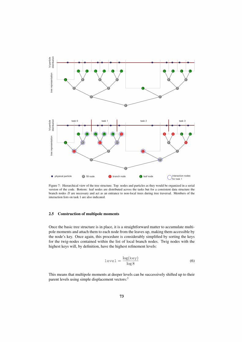
tree
rep
rese
nta
tio
n1
dp
arti
cle
dis
trib
utio
n
L
L L L L L L
L
L L L L
F
F F
F
F
F
F
F
F F
F
P P P P P P P P P P P P
tree
rep
rese
nta
tio
n1
dp
arti
cle
dis
trib
utio
n task0 task1 task2 task3
fillnode branchnode leafnode interactionnodesfortask1
physicalparticleP
P PP PP P P P P P P P P
L
L L L L L L L
B
BB
B
B
B
B
F
F
F
F
F
FF
F
F
F
LB
Figure 7: Hierarchical view of the tree structure. Top: nodes and particles as they would be organized in a serialversion of the code. Bottom: leaf nodes are distributed across the tasks but for a consistent data structure thebranch nodes B are necessary and act as an entrance to non-local trees during tree traversal. Members of theinteraction lists on task 1 are also indicated.
2.5 Construction of multipole moments
Once the basic tree structure is in place, it is a straightforward matter to accumulate multi-pole moments and attach them to each node from the leaves up, making them accessible bythe node’s key. Once again, this procedure is considerably simplified by sorting the keysfor the twig-nodes contained within the list of local branch nodes. Twig nodes with thehighest keys will, by definition, have the highest refinement levels:
level =log(key)
log 8(6)
This means that multipole moments at deeper levels can be successively shifted up to theirparent levels using simple displacement vectors:3
73

∑i qixi → ∑
i qixi − xs∑i qi∑
i qix2i → ∑
i qix2i − 2xs
∑i qixi + x2
s
∑i qi∑
i qixiyi → ∑i qixiyi − xs
∑i qiyi − ys
∑i qixi + xsys
∑i qi,
where rs is the shift vector from the child nodes to their parent.This procedure is continued by working through the sorted list of twigs in reverse
order up to the local branch nodes, which then contain the complete multipole informationfor the local domain. This information is then broadcast to all other processors, so thatthe remaining top-level nodes can be filled in using the shifting rules. At the end of thisprocedure, each processor has the complete multipole expansion for the entire simulationregion contained in the root node.
2.6 Tree traversal
By far the most important and algorithmically challenging part of a parallel tree code is thetree-traversal, which in the present asynchronous implementation requests multipole infor-mation ‘on the fly’ from non-local processor domains. Rather than performing completetraversals for one particle at a time, as many ‘simultaneous’ traversals are made as pos-sible, thus minimizing the duplication incurred when the same non-local multipole nodeis requested many times and maximising the communication bandwidth by accumulatingmany nodes before shipment. In practice, this means creating interaction lists for batchesof around 1000 particles at a time before actually computing their forces. The routinetree walk, which finds the interaction list for each batch has the structure depicted inFig. 8 and Fig. 9.
while any particle not finished walk dofind next node on particle’s walk listif MAC OK then
put node on interaction listwalk-key = next-node
else if MAC not OK for local node thensubdivide: walk-key = first-child
else if MAC not OK for non-local node thenwalk-key = next-nodeput particle on defer listput node on request list
end ifremove finished particles from walk list
end while
Figure 8: Local tree traversal for batch of particles
74

gather request lists for non-local nodes from all processors
for all remote processors doinitiate receive buffer for incoming child datasend off requests for remote child data
end for
for all remote processors dotest for incoming requestpackage and ship back child multipole data to processor that requested it
end for
for all requests doif data has arrived for requested node then
create new hash-table entries for each childend if
end for
copy particle defer lists to new walk lists for next pass through tree
Figure 9: Parallel tree traversal with multipole exchange
In the first, local part of this procedure, traversals are made through the local treeusing the familiar divide-and-conquer strategy common to sequential tree codes17. Themultipole acceptance criterion (MAC) determines whether to accept or subdivide localnodes as usual, but also provides for a third possibility: the subdivision of a non-local nodefor which child data is not yet available. This is then placed on a special ‘request list’ to beprocessed in the 2nd half of the routine when all particles have completed their traversalsas far as they can with the available local node data. Each processor then compiles a list ofnodes it needs child data from, and sends them to the owners of the parent nodes. In the firstpass, these will just be the branch nodes. On receipt of a request list, a processor packagesand ships back the multipole data for the children. The use of non-blocking SENDS andRECEIVES for the multipole information allows some overlap of communication with thecreation of new hash-table entries locally. At the end of all the traversals, each processor’slocal tree contains all the nodes required to compute the forces on its own particles. Thenodes fetched during the traversals can eventually take up most of the space in the localhash-table, as Fig. 10 illustrates.
2.7 Force summation
Once an interaction list has been found for a particle, it is a straightforward task to com-pute its force and potential. Separation of the actual force sum from the tree traversal hasthe advantage that this floating-point-intensive routine can be hardware-optimised. Also,the physics and algorithm are kept naturally apart, so that additional forces, for example,short-range components or magnetic fields and/or corrections due to periodic boundary
75

a) b)
Figure 10: Tree for processor 1, the domain in bottom right quadrant: a) before and b) after traversals for alllocally held particles.
conditions (see next section) can be added with relative ease. In the present implemen-tation, forces are computed for each batch of interaction lists returned from the tree-walkroutine. One subtlety which arises here is that even if overall load-balancing has been ar-ranged during the domain decomposition, it is not necessarily guaranteed for each batchof particles (which may comprise only 1/100 of the total number on each processor). Toredress this problem, the batch size Nb for each processor is determined individually, sothat the integral
Nb∑p=1
Nint(p) (7)
with Nint(p) being the number of interactions of particle p in the previous timestep, is thesame and each processor computes the same number of interaction pairs during each pass.
2.8 Extension to periodic systems
The parallel tree code is capable of simulating systems with large particle numbers. How-ever, for bulk simulations, it is necessary to eliminate surface effects resulting from thesimulation region’s boundaries. This is done by periodic extension of the system to vir-tually infinite size using mirror images of the original simulation box, resulting in twomodifications of the algorithm itself, as denoted in Fig. 11: i) particles leaving the originalsimulation box have to be reinserted on the opposite side, and ii) additional contributionsto the formal force sum for each mirror box at position ~n have to be considered:
~Fi(~r1, . . . , ~rN ; t) =∑~n∈Z3
∑j 6=i
if ~n=0
dd~ri
φ(rij + ~n · L) + ~Fext(~ri; t) . (8)
76

Figure 11: Modification of the algorithm for simulating periodically extended systems: the force acting on aparticle (red) from another one (blue) results from all of its mirror images.
Due to the long-range character of the Coulomb interaction, the box sum cannot betruncated arbitrarily, since it is only conditionally convergent. Additionally, in Eq. 8, theeffective number of interactions grows linearly with the number of mirror boxes and hencecubic with the effective simulation region size. Consequently, a direct summation is com-putationally much too expensive and fast summation schemes are necessary.
The standard Ewald method18, 19, i.e. splitting the box sum into a real and a Fourierspace part is not used for periodic extension in PEPC, since its convergence and accuracyare rather difficult to control and it would have to be applied to each particle separately.
Instead, an elegant approach borrowed from the fast multipole method2, 20 is adoptedhere. It is based on the bipolar expansion of the inverse distance in terms of Legendrepolynomials:
1
|~a2 − ~a1 + ~n| =
∞∑l=0
l∑m=−l
∞∑j=0
j∑k=−j
(−1)j Oml (~a1)Mm+kl+j (~n)Okj (~a2) (9)
77
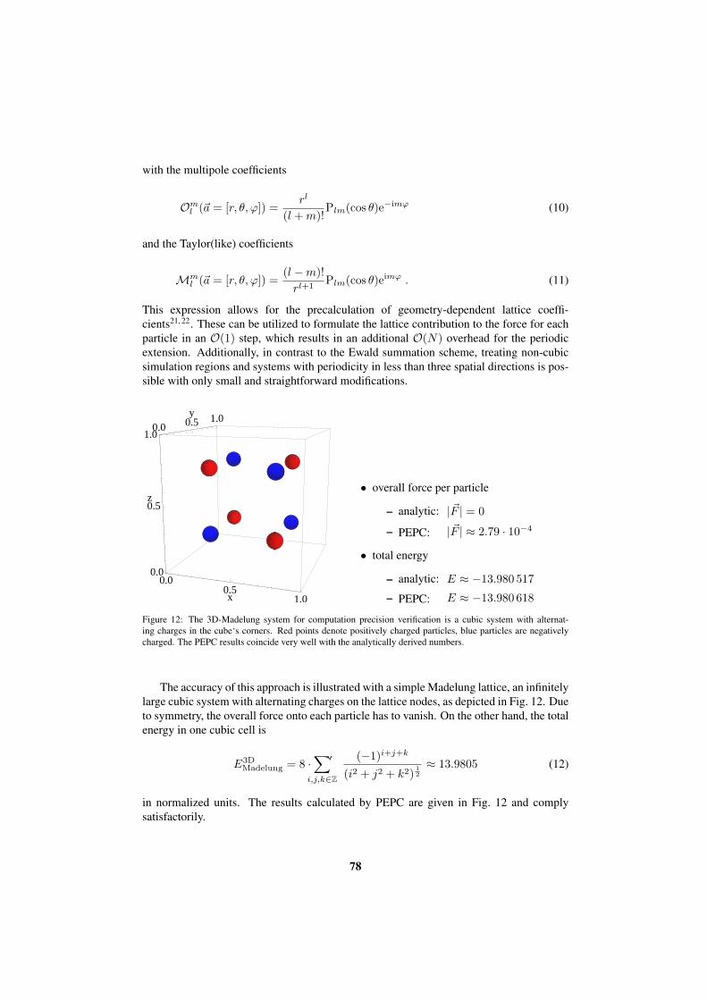
with the multipole coefficients
Oml (~a = [r, θ, ϕ]) =rl
(l +m)!Plm(cos θ)e−imϕ (10)
and the Taylor(like) coefficients
Mml (~a = [r, θ, ϕ]) =
(l −m)!
rl+1Plm(cos θ)eimϕ . (11)
This expression allows for the precalculation of geometry-dependent lattice coeffi-cients21, 22. These can be utilized to formulate the lattice contribution to the force for eachparticle in an O(1) step, which results in an additional O(N) overhead for the periodicextension. Additionally, in contrast to the Ewald summation scheme, treating non-cubicsimulation regions and systems with periodicity in less than three spatial directions is pos-sible with only small and straightforward modifications.
0.00.5
1.0x
0.0 0.5 1.0y
0.0
0.5
1.0
z• overall force per particle
– analytic: |~F | = 0
– PEPC: |~F | ≈ 2.79 · 10−4
• total energy
– analytic: E ≈ −13.980 517
– PEPC: E ≈ −13.980 618
Figure 12: The 3D-Madelung system for computation precision verification is a cubic system with alternat-ing charges in the cube‘s corners. Red points denote positively charged particles, blue particles are negativelycharged. The PEPC results coincide very well with the analytically derived numbers.
The accuracy of this approach is illustrated with a simple Madelung lattice, an infinitelylarge cubic system with alternating charges on the lattice nodes, as depicted in Fig. 12. Dueto symmetry, the overall force onto each particle has to vanish. On the other hand, the totalenergy in one cubic cell is
E3DMadelung = 8 ·
∑i,j,k∈Z
′ (−1)i+j+k
(i2 + j2 + k2)12
≈ 13.9805 (12)
in normalized units. The results calculated by PEPC are given in Fig. 12 and complysatisfactorily.
78

3 Algorithm Scaling and Performance
The adaption of an algorithm to massively parallel systems (thousands of tasks) creates amultitude of challenges. In general, these differ from those which arise at scales of only afew tasks. E.g. in the case of strong scaling at large scales, all components which have aconstant or even a P dependent complexity must be avoided. However, some algorithmsmight depend on non-scaling actions, like collective communication in PEPC, and willhave to be optimized.
Initialise particle properties ri,vi, qi,mi N/PKey construction: (xi, yi, zi)→ ki N/PSort keys: k1, k2, ...kN N/P logNDomain decomp.: k1, ..kn; kn+1, ..k2n; ...; kN−n...kN N/PConstruct branch nodes P logN/PFill in top level local tree nodes logPBuild multipole moments logN/PConstruct interaction lists (tree traversal) N/P logNCompute forces and potential N/P logNUpdate particle velocities and positions N/P
Table 1: Algorithmic scaling of major routines in PEPC. The symbols N and P represent the total number ofparticles and processors respectively, and n = N/P .
The overall algorithm is depicted together with the theoretical scaling of each majorroutine in Table 1. We see that in principle, all of the above routines can be performed inparallel, and thus require a computational effort O(N/P ), give or take a slowly varyinglogarithmic factor. Single-timestep benchmarks with this new code broadly confirm thetheoretical scalings indicated in Table 1. As expected, most of the time is spent in the tree-traversal and force-summation routines: the total overhead incurred by the tree construction(which includes the steps 2.3, 2.3 and 2.4 described previously) is around 3%, although thisfigure excludes tree-nodes copied locally during the traversal—Table 2.
Routine/ No. CPUs 8 16 64
Domain decomposition 0.2 0.24 0.33Tree building 2.3 2.3 2.7Tree traversal 32.9 36.1 40.8Force summation 64.4 61.2 55.7
Table 2: Breakdown of relative computational effort (percentage of wall-clock time spent in each routine) in theparallel tree code for a test case with 100k particles and 8, 16 and 64 processors respectively on a PC cluster
79

The first part of this section demonstrates PEPC’s scaling on a massive parallel system,IBM Blue Gene/P Jugene at the Julich Supercomputing Centre. To our knowledge, theachieved scaling is exceptional among the currently available tree codes23, 24. For strongscaling, there is unavoidably a maximal number of tasks up to which a speedup can begained, due to essential non-scaling elements: sorting of particles and global informationexchange. Even if unconditional strong scaling is currently not possible, it is important toensure optimal efficiency of all application’s parts to be able to reach the highest scales.Therefore, the following sections give an insight in the efficiency of the communicationstrategy and the parallel sorting routine, as well as the identification of one of the currentbottle necks: the P -dependency of the number of branch nodes.
The PEPC code is written in a generic fashion without the usage of external libraries.This results in excellent portability. In the PRACE benchmarking framework. PEPC wasrun on four different computer architectures, namely: IBM Blue Gene/P (jugene), IBMPower6 (huygens), Cray XT5 (louhi), Intel Nehalem (juropa).
Figure 13 shows strong scaling results from 1 to 8192 mpi tasks on Jugene. We haveused four different datasets since the number of particles per task for PEPC is bound by 105
on Jugene. To this end we used 1×10⁵, 1.6×10⁶, 2.56×10⁷ and finally 1×10⁸ particles todemonstrate PEPC’s capabilities. As these runs show our implementation is able to use upto 8192 mpi tasks very efficiently with adequate datasets. The scaling behavior is very goodfor 1 to 4096 mpi tasks yielding more than 3 orders of magnitudes of speedup. Especiallyfor a high number of particles per task the code scales nearly perfectly. However, loweringthis ratio detaches the scaling from the ideal linear speedup. Furthermore, the appearanceof this phenomenon is not only coupled to the ratio of particles per tasks but also on thenumber of tasks itself: the scaling behaviour is much better for small than for large datasets.
1 2 4 8 16 32 64 128 256 512 1024 2048 4096 8192tasks
1
4
16
64
256
1024
4096
rela
tive
spee
dup
1 · 105 particles1 · 106 particles3 · 107 particles1 · 108 particles
Figure 13: Hybrid scaling for various homogeneous datasets on IBM Jugene, strong scaling for each dataset.
80

To analyse this behavior, Figure 14 shows the detailed timings on the large datasetfor each of the four major steps involved in the one iteration of the algorithm illustratedin Fig.1. It becomes clear that these steps behave very differently for larger number oftasks. While the time-consuming tree traversal and force calculation steps show perfectstrong scaling the domain decomposition and tree construction are clearly responsible forits saturation at this level. Since steps 1 and 2 do not scale at all, they start to dominate thecalculation time at 8192 tasks in this case.
256 512 1024 2048 4096 8192tasks
100
101
102
tim
e[s
]
totalstep 1step 2step 3step 4
Figure 14: Detailed timings on IBM Jugene for 2.56 × 10⁷ particles in a cube, split into the four main stepsof PEPC: domain decomposition (step 1), tree construction (step 2), tree traversal (step 3) and force calculation(step 4)
Both steps 1 and 2 include collective operations: the domain decomposition duringparallel sorting, the tree construction for the branch exchange process. Furthermore, theamount of data exchanged during these operations increases with the number of tasks. Thebranch structure becomes a particular problem at high task numbers. Each task definesat least one branch – but typically up to 30 – for its local particles, which have to bepropagated to all other tasks – see Fig. 5. Moreover, the branch level inside the tree – andthereby the total number of branches – increases during a strong-scaling scenario, i.e. fora fixed problem size with variable number of tasks. In addition, the underlying structure ofglobal fill nodes (see Fig. 7) increases as well, so that this step takes more time, too. Theconsequences and costs arising from the branch structure therefore are responsible for thelack of scaling of step 2.
While parallel sorting and reordering of the particles during step 1 is a necessary andinevitable part of tree codes and is already implemented very efficiently, it is interesting toask how the branch- and fill-node structure affect the interaction list generation and forcecalculation. Detailed analyses25 reveal that nearly all of the local and fetched nodes appearat least once on an interaction list, but with increasing number of tasks the proportionof used remote branches and even used fill nodes tends to zero. While the first result
81

demonstrates the efficiency of the implemented traversal strategy in PEPC – since nearly nonode is fetched but unused, the second result indicates that branch and top level fill nodesthemselves are generally redundant with respect to force calculation. On the one handthe tree construction step suffers from branch exchange and global node creation processconsuming a significant amount of memory and communication-time, while on the otherhand theses structures have virtually no impact on the force calculation. Further analysisshows that these results do not depend significantly on the particle distribution. Even forPlummer-like distributions26 the role of the global tree structures is negligible with respectto the interaction lists. But in the same way the traversal efficiency remains very close to100%, which is a very good result. Therefore, a starting-point for future optimization ofefficiency, memory consumption and scaling would be to optimise the branch structure.
Moreover, an important further issue which must be addressed at such high concur-rency levels before the code can be usefully applied to real physics problems is parallelI/O. The main output from PEPC takes the form of regular particle dumps containing theirproperties (coordinates, velocities, keys, labels and possibly local field information). Theseare used both for checkpointing (restarting the code mid-simulation) and for postprocess-ing purposes. Like any other particle code, a bottleneck is created if this data first has tobe gathered or distributed among a few thousand tasks. Rather than relying on parallelversions of standard portable data formats (HDF5, netcdf, MPI-I/O), we have deployed anew scalable I/O library for writing code data – SIONlib – developed at JSC27. Using thisformat, particle data is written to and read from a single ‘task-local’ binary file at eachcheckpoint. Postprocessers equipped with SIONlib are also speeded up considerably.
4 Summary and Outlook
In this paper we have described our parallel tree code PEPC and demonstrated its capa-bilities on an IBM Blue Gene/P system, simulating many-million particle systems. Withits highly optimized traversal routine this code scales exceptionally well up to 4096 tasksproviding library users with a very flexible, portable and mesh-free algorithm for plasmaphysics, Newtonian gravity and vortex methods. However, as our benchmarks have shown,the collective operations during domain decomposition and the tree construction processinduce a significant overhead. While parallel sorting is an inevitable part of a tree code adetailed analysis of the tree data structure proved the efficiency of the traversal, but alsoindicated a massive redundancy of branch and global nodes.
As a consequence, our current focus is on a interaction list prediction method to avoidthe explicit storage of unused nodes during tree construction. By abstracting the branchconcept we hope to optimize PEPC’s memory footprint significantly, clearing the way foreven larger datasets beyond 109 particles and scaling well beyond 104 tasks.
References
1. J. Barnes and P. Hut, A hierarchicalO(N logN) force-calculation algorithm, Nature,324, 446–449, (1986).
2. L. Greengard and V. Rokhlin, A fast algorithm for particle simulations, J. Comp.Phys., 73, 325–348, (1987).
82

3. S. Pfalzner and P. Gibbon, Many Body Tree Methods in Physics, Cambridge Univer-sity Press, New York, (1996), ISBN 0-521-49564-4 (hardback); ISBN 0-521-01916-8(paperback).
4. V. Springel, N. Yoshida, and S. D. M. White, GADGET: A code for collisionless andgasdynamical cosmological simulations, New Astronomy, 6, 79–117, (2001).
5. P. Gibbon, W. Frings, S. Dominiczak, and B. Mohr, Performance analysis and visu-alization of the N -body tree code PEPC on massively parallel computers, in: Proc.Parallel Computing 2005, Malaga, G. Joubert and et al., (Eds.), vol. 35, NIC Series,Forschungszentrum Julich, Julich, (2006).
6. PEPC can be obtained from: https://trac.version.fz-juelich.de/pepc7. P. Gibbon, R. Speck, A. Karmakar, L. Arnold, W. Frings, B. Berberich, D. Reiter and
M. Masek, Progress in Mesh-Free Plasma Simulation With Parallel Tree Codes, IEEETransactions on Plasma Science, 38, 2367–2376 (2010).
8. P. Gibbon, F. N. Beg, R. G. Evans, E. L. Clark, and M. Zepf, Tree code simulationsof proton acceleration from laser-irradiated wire targets, Phys. Plasmas, 11, 4032–4040, (2004).
9. M. S. Warren and J. K. Salmon, A portable parallel particle program, Comp. Phys.Commun., 87, no. 266–290, (1995).
10. U. Becciani, V. Antonuccio-Delogu, and M. Gambera, A modified parallel tree codefor N -body simulation of the large-scale structure of the universe, J. Comp. Phys.,163, 118–132, (2000).
11. J. Dubinski, A parallel tree code, New Astronomy, 1, 133–147, (1996).12. H. Yahagi, M. Mori, and Y. Yoshii, The forest method as a new parallel tree method
with the sectional voronoi tessellation, Ap. J. Supp., 124, 1–9, (1999).13. M. S. Warren and J. K. Salmon, A parallel hashed oct-tree N -body algorithm, in:
Supercomputing ’93, pp. 12–21, IEEE Comp. Soc., Los Alamitos, (1993).14. H. Sagan, Space-Filling Curves, Springer, Heidelberg, (1994).15. H. Shi and J. Schaeffer, Parallel sorting by regular sampling, J. Par. Dist. Comp., 14,
361–372, (1992).16. M. Hofmann, G. Runger, P. Gibbon, and R. Speck, Parallel sorting algorithms for
optimizing particle simulations, IEEE Cluster, (2010, in press).17. S. Pfalzner and P. Gibbon, A hierarchical tree code for dense plasma simulation,
Comp. Phys. Commun., 79, 24–38, (1994).18. P. P. Ewald, Die Berechnung optischer und elektrostatischer Gitterpotentiale, Ann.
Phys., 64, 253–287, (1921).19. M. J. L. Sangster, M. Dixon, Interionic potentials in alkali halides and their use in
simulations of the molten salts, Adv. Phys., 25, 247–342, (1976).20. I. Kabadshow, The Fast Multipole Method – Alternative Gradient Algorithm and Par-
allelization, Diploma Thesis, Forschungszentrum Julich, jul-4215, ISSN 0944-2952(2006).
21. M. Challacombe, C. White, M. Head-Gordon, Periodic boundary conditions and thefast multipole method, J. Chem. Phys., 107, 10131–10140, (1997).
22. K. N. Kudin, G. E. Scuseria, Revisting infinite lattice sums with the periodic fastmultipole method, J. Chem. Phys., 121, 2886–2890, (2004).
23. B. Jeon, J. D. Kress, L. A. Collins, and N. Groenbech-Jensen, Parallel Tree code fortwo-component ultracold plasma analysis, Comp. Phys. Commun., 178, 272–279,(2008).
83

24. A. F. Nelson, M. Wetzstein, and T. Naab, Vine – A numerical code for simulatingastrophysical systems using particles II: Implementation and performance character-istics, Ap. J. Supp. Series, 184, 326–360, (2009).
25. R. Speck, P. Gibbon, and M. Hoffmann, Efficiency and scalability of the paralleBarnes-Hut tree code PEPC, in: Parallel Computing (ParCo), (2009).
26. S. J. Aarseth, M. Henon, and R. Wielen, Comparison of numerical-methods for studyof star cluster dynamics, Astronomy and Astrophysics, 37, no. 1, 183–187, (1974).
27. W. Frings, F. Wolf, and V. Petkov, Scalable massively parallel I/O to task-local files,in: Proc. of the ACM/IEEE Conference on Supercomputing (SC09), pp. 1–11, ACM,Portland, OR, (2009).
84

The Error-Controlled Fast Multipole Method for Openand Periodic Boundary Conditions
Ivo Kabadshow and Holger Dachsel
Institute for Advanced SimulationJulich Supercomputing Centre
Forschungszentrum Julich, 52425 Julich, GermanyE-mail: i.kabadshow, [email protected]
The simulation of pairwise interactions in huge particle ensembles is a vital issue in scientificresearch. The calculation of long-range interactions poses limitations to the system size, sincethe number of these interactions scales quadratically with the number of particles. Fast sum-mation techniques like the Fast Multipole Method (FMM) can help to reduce the complexityto O(N). In this article we describe the basic ideas behind the FMM for open boundary con-ditions, as well as the extension of the FMM to (mixed) periodic boundaries. Together with atight error control, this scheme enables the simulation of particle systems for different applica-tions without the need to know and tune the FMM specific parameters. The implemented errorcontrol scheme automatically optimizes the parameters to obtain a minimal calculation time fora given energy error bound ∆E.
1 Introduction
The main idea behind fast summation methods, especially the FMM, is to give an ap-proximate solution within a given precision goal ε of a certain quantity (energy, forces,potentials). However, this precision goal ε could be machine precision in which case theapproximate solution does not differ from the “exact solution” when computed numeri-cally.
The presented approximation will benefit from the following observation. Assume asystem of several clustered particles. The contribution on the force or energy, respectivelyfrom nearby particles on a test particle within a cluster will be dominant compared to thecontribution from remote particles outside the cluster. Admittedly, the remote contribu-tion is not zero. Neglecting these particles would correspond to a cut-off scheme withoutrigorous error control but ideal complexity O(N).
Grouping Source Particles
However, a remote particle from a spatial group will have almost the same influence onthe test particle near the origin as another particle from the same remote group, sincethe distance between the test particle at the origin and the remote particles is dominatedby a large cluster–cluster distance. Therefore, all particles in a remote cluster could becombined together and may be represented by a new single pseudo particle with a newcommon center. The influence of several sources is combined into one source, which isdepicted in figure 1b.
85

(a) 56 Direct Interactions (b) 8 Interactions:Grouped Source Particles
(c) 7 Interactions:Grouped Target Particles
(d) 1 Interaction:Grouped Source & TargetParticles
Figure 1: The figure depicts the main idea behind fast summation methods with respect to a particle system.The particles are randomly distributed in space, but show clustering. Chart (a) shows the direct interaction of allparticles in one cluster with all particles in the other cluster. Inter-Cluster interactions are not shown. Chart (b)shows the interaction via a source pseudo particle. Chart (c) shows the interaction via a target pseudo particle.Chart (d) shows the interaction with both, source and target pseudo particles.
Grouping Target Particles
The grouping scheme can also be used in reverse. Considering a remote particle and agroup of particles clustered together near the origin, the remote particle has almost thesame influence on any source particle in the spatial group. Therefore, the interaction ofthis remote particle can be reduced to the interaction with a pseudo particle containing theclustered source particles (see figure 1c).
Grouping Both Source and Target Particles
Finally, the last two schemes can be combined together, allowing interactions of twopseudo particles, one at source and one at target particles. This scheme is depicted infigure 1d. Interaction takes place only via pseudo particles and not particles itself. Thisis advantageous since all particles in a simulation are sources and targets at the same timedue to the mutual interaction. Hereby the number of interactions between the particles isreduced even more compared to asymmetric clustering of either source or target points.
Defining Groups of Different Size
To define near and remote particles, a space decomposition scheme is used. For reasonof simplicity we assume a recursive decomposition in cubic boxes. The different sizedboxes are stored in a tree-like (oct-tree) data structure providing efficient construction ofinteraction sets, since source and target sets can be increased in size the more distant theyare.
To generate the source and target sets from the given particle distribution, two operatorsare necessary. We distinguish between operators working vertically and horizontally insidethe tree. First, the vertical operators shift expansions of source or target sets up and downthe tree. Second, the horizontal operator translates source sets into target sets on each treelevel.
86

(a) Interaction Matrix (b) FMM Interaction Matrix (c) Direct and Clustered Interac-tions
Figure 2: Figure (a) depicts the interaction matrix of the direct interaction. Figure (b) depicts the interactionmatrix via the FMM. Each square represents a certain particle-particle or multipole-multipole interaction.Figure(c) depicts the direct interaction (first line) of a 1D system with 16 elements (black circles) and the interaction viathe FMM scheme.
However, it is possible that a limited number of nearby particles is not able to interactvia pseudo particles. Therefore, these particles interact directly with each other. Thisrestriction can be avoided by very deep trees, hence a very fine spatial decompositionwhere each particle has its own box. But this is not necessary, since the number of nearbyparticles is limited and thus does neither impair the overall complexity nor the computationtime.
Interaction Sets
Figure 2a shows the interaction matrix of 16 particles. Every cell represents a single in-teraction pair. The crossed out cells represent interactions from particles with themselveswhich must not be calculated (singularity) and are dropped eventually. The first interactionmatrix in figure 2a represents all N(N − 1) interactions. Due to symmetry, the lower lefthalf contains the exact same elements of the upper half. Thus, the overall interactions re-duce to 1
2N(N − 1). The second interaction matrix in figure 2b represents the interactionof the same particles via an FMM computation. Again, the crossed out cells are omitted.The dark-grayed cells represent direct neighbors, which have to be calculated directly. Theremaining cells represent interactions via pseudo particles. The streaked cells are shownseparately with their interaction sets in figure 2c. One can easily see, that with increasingdistance more and more source and target particles are grouped together which reduces thenumber of interactions dramatically. Again, the lower triangle is symmetric to the uppertriangle similar to the direct summation. To establish an accurate algorithm, providing thementioned features, we need to introduce additional mathematical tools. In the next sectionwe will derive the necessary theorems.
87
2 Fast Multipole Method for Open Boundaries
2.1 Mathematical Preliminaries
In three dimensions, functions which satisfy the Laplace equation
∇2Φ =∂2Φ
∂x2+∂2Φ
∂y2+∂2Φ
∂z2= 0
are referred to as harmonic functions. The theory of such functions is called potentialtheory. A description of the theory can be found in1. A solution satisfying the Laplaceequation is e.g. Φ = 1/d with d =
√(x− x0)2 + (y − y0)2 + (z − z0)2.
If a point particle of unit strength is fixed at A = (x0, y0, z0) then the potential due tothis charge at an arbitrary but distinct point R = (x, y, z) is given by
Φ(R) =1
d
with d representing the distance between point R and A. The electrostatic field is given by
~E(R) = −∇Φ = −(x− x0
d3,y − y0
d3,z − z0
d3
)T.
Next we want to derive a series expansion for the potential at R in terms of the distancefrom the origin r.
2.2 Expansion of the Inverse Distance
Given two points A(a, α, β) and R(r, θ, φ) with a, α, β and r, θ, φ being the sphericalcoordinates, we define the distance d as
d := |r− a| =√r2 + a2 − 2ra cos γ .
Thus,
1
d=
1
r√
1− 2ar cos γ + a2
r2
=1
r√
1− 2uµ+ µ2,
having set
µ =a
rand u = cos γ .
For µ ≤ 1, the inverse square root can be expanded in powers of µ, resulting in the follow-ing series
1√1− 2uµ+ µ2
=∞∑l=0
Pl(u)µl ,
where
P0(u) = 1, P1(u) = u, P2(u) =3
2(u2 − 1
3), . . . .
88

Figure 3: Expansion of the inverse distance 1/d into the radial parts a and r and the subtended angle γ betweenOA and OR.
In general, the Pl(u) are the Legendre polynomials2 of degree l and are defined by
Pl(x) =1
2ll!
dl
dxl[(x2 − 1)l
].
Finally the expression for the inverse distance 1/d yields
1
d=
1
r
∞∑l=0
al
rlPl(u) =
∞∑l=0
al
rl+1Pl(cos γ) . (1)
The radial parts a and r of the two coordinates a and r are now factorized.
2.3 Spherical Harmonic Addition Theorem
Unfortunately, Pl(cos γ) does still depend on both coordinates A and R via cos γ andcannot be used to derive a fast summation scheme. A useful representation requires theintroduction of spherical harmonics, allowing to factorize both source and target locations.By transforming the Laplace equation in spherical coordinates (see figure 4a), we get
1
r2
∂
∂r
(r2 ∂Φ
∂r
)+
1
r2 sin θ
∂
∂θ
(sin θ
∂Φ
∂θ
)+
1
r2 sin2 θ
∂2Φ
∂φ2= 0 .
The solution of the equation can be found by assuming a separable solution of the form
Φ(r, θ, φ) = R(r)T (θ)P (φ)
leading to an expression including spherical harmonics Ylm and coefficients Mlm and Llm
Φ(r, θ, φ) =∞∑l=0
l∑m=−l
LlmYlm(θ, φ)rl +MlmYlm(θ, φ)
rl+1.
Remark 2.1. It should be noted that for a potential ΦO(r, θ, φ) with r > a, the coefficientsLlm have to be zero to satisfy the decay at infinity for the potential ΦO as shown in figure4b. For the potential ΦI(r, θ, φ) with r ≤ a inside the sphere with radius a the elementsMlm must be zero. (see figure 4c).
89

θ
φy
x
z
r
~re
~φe
~θe
x
y
z
(a) Spherical coordinate system (b) Analytic domain of a multi-pole expansion of the potentialΦO with r > a
(c) Analytic domain of a local ex-pansion of the potential ΦI withr < a
Figure 4: The solution for the potential Φ(r, θ, φ) consists of two separate solutions. The domain can be splitinto two distinct parts. First, the local part inside the sphere. Second, the external part outside the sphere.
2.4 Expansion of Particle-Particle Interactions
Following the notation of Head-Gordon3 and the derived formulas from the last sections,we can expand the coordinates of a particle-particle interaction as follows
1
|r− a| =
∞∑l=0
Pl(cos γ)al
rl+1
=∞∑l=0
l∑m=−l
(l −m)!
(l +m)!
al
rl+1Plm(cosα)Plm(cos θ)e−im(β−φ) .
We define the scaled associated Legendre polynomials Plm and ˜Plm to ensure numericalstability and to simplify the FMM operators with
Plm =1
(l +m)!Plm and ˜Plm = (l −m)!Plm .
Now, we define the multipole moments ωjlm(qj ,aj) for a particle at aj with strength qjabout the origin (0, 0, 0). The chargeless version of the multipole is defined by Ojlm(aj)with
ωjlm(qj ,aj) = qjOjlm(aj) = qja
ljPlm(cosαj)e
−imβj .
Multipole moments of multiple particles j ∈ 1, . . . , k about a common origin can besummed, yielding
ωlm(q,a) =k∑j=1
ωjlm(qj ,aj) =k∑j=1
qjOjlm(aj) =
k∑j=1
qjaljPlm(cosαj)e
−imβj .
We can also establish the coefficients of a local Taylor-like expansion of the potential atthe origin due to a distant particle at rj . The chargeless version of the local Taylor-like
90
expansion is defined by M jlm(rj) as
µjlm(qj , rj) = qjMjlm(rj) = qj
1
rl+1j
˜Plm(cos θj)eimφj .
Again, coefficients with a common origin can be summed
µlm(q, r) =k∑j=1
µjlm(qj , rj) =k∑j=1
qjMjlm(rj) =
k∑j=1
qj1
rl+1j
˜Plm(cos θj)eimφj .
We denote chargeless multipole expansions Olm and chargeless Taylor-like expansionsMlm for k = 1 without the superscript j, subsequently. The corresponding potential Φ(P )due to a set of particles can be defined via the following two theorems.Theorem 2.2. Multipole expansion Suppose that k particles of strengths qj , j = 1, . . . , kare located at the points aj = (aj , αj , βj), j = 1, . . . , k with |aj | < a inside a sphere.Then for any P = (r, θ, φ) ∈ R3 with r > a, the potential Φ(P ) is given by
Φ(P ) =
∞∑l=0
l∑m=−l
ωlm(q,a)1
rl+1˜Plm(cos θ)eimφ
=∞∑l=0
l∑m=−l
ωlm(q,a)Mlm(r) .
Theorem 2.3. Local expansion (Taylor-like) Suppose that k particles of strengths qj , j =1, . . . , k are located at the points Rj = (rj , θj , φj), j = 1, . . . , k outside the sphere withradius a with a < rj . Then for any P = (a, α, β) ∈ R3 with a < a, the potential Φ(P ) isgiven by
Φ(P ) =∞∑l=0
l∑m=−l
µlm(q, r)alPlm(cosα)e−imβ
=∞∑l=0
l∑m=−l
µlm(q, r)Olm(a) .
2.5 Mathematical Operators
In this section we describe the FMM operators, which can be derived from the preliminariesof the last section to obtain a fast summation scheme. We need three different operators toestablish the FMM scheme. Two operators for the vertical up- and down-shifts between thedifferent tree levels and one operator for the conversion of remote multipole expansions ateach tree level.
2.5.1 Translation of a Multipole Expansion (M2M)
With help of an addition theorem4 we are able to shift the coefficients of a multipole ex-pansion around a point located at a to a point located at a + b (Fig 5) yielding
Olm(a + b) =l∑
j=0
j∑k=−j
Ojk(a)Ol−j,m−k(b) .
91

(a) Analytic Domain (b) Tree View
Figure 5: M2M operator for a two dimensional system. M2M is a vertical operator, exchanging informationbetween levels.
The addition theorem allows us to factorize the potential 1/|r − (a + b)| into a sum oftriple products depending separately on r, a and b as follows
1
|r− (a + b)| =∞∑l=0
l∑m=−l
Olm(a + b)Mlm(r)
=∞∑l=0
l∑m=−l
l∑j=0
j∑k=−j
Ojk(a)Mlm(r)Ol−j,m−k(b) .
The derivation for the multipole expansions ωlm is straightforward
ωlm(a + b) =l∑
j=0
j∑k=−j
ωjk(a)Ol−j,m−k(b) .
We identify operator A with
Almjk (b) = Ol−j,m−k(b). (2)
This operator is also called Multipole2Multipole operator or M2M. Operator A is free oferrors. Independent of the length of the multipole expansion, all shifted moments are exactsince the operator only includes elements up to the order of the shifted ones. The M2Moperator is a vertical operator acting on boxes of different tree levels.
2.5.2 Conversion of a Multipole Expansion into a Local Expansion (M2L)
With help of another addition theorem4 we are able to transform an external multipoleexpansion into a local Taylor-like expansion. The chargeless version of the operator yields
Mlm(b− a) =∞∑j=0
j∑k=−j
Ojk(a)Mj+l,k+m(b) .
Similarly to the first FMM operator we can substitute the termsOlm andMlm to obtain thecharged version of this operator. Now, we are able to transform coefficients of an external
92

(a) Analytic Domain (b) Tree View
Figure 6: M2L Operator for a two dimensional system. M2L is a horizontal operator, exchanging informationbetween boxes of the same level.
multipole expansion around a to local Taylor-like coefficients around (b− a) as shown infigure 6. The transformed Taylor-like expansion can be represented as
µlm(b− a) =∞∑j=0
j∑k=−j
Mj+l,k+m(b)ωjk(a)
with Multipole2Local (M2L) operator
Blmjk (b) = Mj+l,k+m(b) . (3)
Besides errors arising from the truncation of the expansion ωjk with j ≤ p, additionaloperator errors are introduced, because only 2p terms are considered in the sum for theelements Mj+l,k+m with j + l ≤ 2p. Since the operator itself is expanded up to 2pit allows to transform all available elements in ωjk. The M2L operator is a horizontaloperator acting on boxes of the same tree level.
2.5.3 Translation of a Local Expansion (L2L)
The last operator can be obtained by using the first addition theorem again. With the helpof the factorized potential, given by
1
|r− (a + b)| =∞∑l=0
l∑m=−l
Olm(a + b)Mlm(r)
=∞∑l=0
l∑m=−l
l∑j=0
j∑k=−j
Ojk(a)Mlm(r)Ol−j,m−k(b) ,
and the manipulation scheme for a double summation from reference5 with elements
Ajl(a,b, r) =l∑
m=−l
j∑k=−j
Ojk(a)Mlm(r)Ol−j,m−k(b)
93

(a) Analytic Domain (b) Tree View
Figure 7: L2L Operator for a two dimensional system. L2L is a vertical operator, exchanging information betweenlevels.
we can change the order of the summation
1
|r− (a + b)| =
∞∑l=0
l∑j=0
Ajl(a,b, r) =
∞∑j=0
∞∑l=j
Ajl(a,b, r) .
Relabeling the indices l ↔ j,m ↔ k of the last equation and resubstituting the originalmultipole and Taylor-like expansion yields
1
|r− (a + b)| =
∞∑l=0
∞∑j=l
l∑m=−l
j∑k=−j
Olm(a)Mjk(r)Oj−l,k−m(b) .
Separating the terms Oj−l,k−m and Mjk results in the operator C, which allows us totranslate a Taylor-like expansion located around r to its center at (r − b) as shown infigure 7 with
Mlm(r− b) =
p∑j=l
j∑k=−j
Oj−l,k−m(b)Mjk(r) .
This operator is also called Local2Local (L2L) operator. Compared to operatorA, this op-erator introduces errors due to the finite representation of the multipole expansion. How-ever, compared to operator B no additional operator errors arise. For a finite Taylor-likeexpansion with a truncation at p poles the operator is exact with respect of the length of theTaylor-like expansion. The operator L2L is used to shift finite Taylor-like moments from aparent box to its children boxes’ centers. The charged version of the operator is given by
µlm(r− b) =
p∑j=l
j∑k=−j
Oj−l,k−m(b)µjk(r)
with L2L operator
Clmjk (b) = Oj−l,k−m(b) . (4)
The L2L operator is a vertical operator acting on boxes of different tree levels.
94

Operator Purpose Truncation Error Additional Operator Error
A Multipole to Multipole — —B Multipole to Local • •C Local to Local • —
Table 1: The three FMM operators have different sources of error. The most error-prone operator is operatorB. To derive valid error estimation schemes, the influence of operator B must be considered additionally to thetruncation errors introduced by the finite expansion.
Remark 2.4. Omitting operator M2M and L2L increases the complexity to O(N logN).Such a scheme would behave like a Barnes-Hut treecode6, but with improved prefactor.
Obviously all operators induce a complexity of O(p4). Especially high precision cal-culations are slowed down. To overcome this problem, improvements to the operators havebeen proposed.
2.5.4 Rotation-Based Operators
To circumvent the O(p4) operator scaling, White and Head-Gordon7 proposed a differentscheme improving the operator scaling to O(p3). The improved scheme is easy to im-plement with the proposed standard FMM operators and only needs minor modifications.The increased memory usage is negligible and no additional approximations are induced.The original error bounds are retained. The rotation based operators are predicated on theobservation that the three dimensional problem is reduced to a one dimensional problem ifthe translation or shift is carried out along the quantization axis (z-axis). Wigner rotationmatrices are applied to rotate the multipole moments. A shift along the quantization axiswith θ = 0 and φ = 0 yields a simplified form for the representation of the chargelessmultipole moments with
Olm(a) =1
(l +m)!alδm0
Mlm(r) = (l −m)!1
rl+1δm0 .
Simple rotations preserve the total angular momentum. Therefore, any rotated sphericalharmonic will be given as a linear combination of other spherical harmonics having thesame order p. The implementation of the FMM presented here is based on these rotation-based operators.
2.6 O(N logN) Algorithm
In this section we describe the details of the simpler algorithm not using any translationoperators which yields an overall complexity of O(N logN). However the final FMMscheme can be based on this approach. We start to enclose our given particles inside a cubeand call this box simulation box. Next, we introduce a hierarchy of boxes by subdividingthis simulation box at half along each axis. The refinement level of the entire simulation
95

(a) Level 1 – Depth 0 (b) Level 2 – Depth 1 (c) Level 3 – Depth 2 (d) Level 4 – Depth 3
Figure 8: The FMM tree is subdivided until a certain number of particles on the lowest level is reached. LevelL = 1 corresponds to the highest level, level Lmax corresponds to the lowest level. The subdivision shown, addsfour times the number of boxes to the tree for each level. In three dimensions, the number of boxes increases bya factor of 8.
box is named level one (L = 1). An arbitrary level of refinement L+ 1 can be obtained bysubdividing each box at level L into eight equal subboxes. The 8L subboxes at level L+ 1are called child boxes of their parent box at refinement level L. The scheme correspondsto the construction of an oct-tree depicted in figure 8.
Now we can derive subsets of boxes via the following definitions.Definition 2.1. Two boxes A and B are called next neighbors if they are at the same treelevel and box B is enclosed by a box of size (2ws+ 1)3 around the center of A with a boxedge length of one. Next neighbors interact in the near field (NF).
The former definition allows us to increase the range for the near field part to the fullsimulation box (ws → ∞) yielding a direct interaction scheme with O(N2) complexity.A definition for a minimal ws = 1 criterion can be written as follows:Definition 2.2. Two boxes are called next neighbors if they are at the same tree level andshare a boundary point (see figure 9b). Next neighbors interact in the near field (NF).
After defining the near field, the far field has to be defined accordingly.Definition 2.3. Two boxes A and B are called well separated if they are at the same treelevel and are not next neighbors (see figure 9c). Well separated boxes interact in the farfield (FF).
The last definition does not limit the number of interactions in the far field, thereforewe have to set up a confined interaction list.Definition 2.4. An interaction list i is associated with each box A, consisting only of chil-dren of the next ws neighbors of A’s parent which are well separated from box A (see figure9d). The interaction list limits the number of far field (FF) interaction for each box.
These definitions allow us to compute interactions between a constant number of boxeson each level. The spatial refinement enables us to cluster together particles from one andthe same box into multipole moments. The expansion of the particles is performed aroundthe box center. With the help of definition 2.4 it is possible to define interaction sets formultipole expansions of these boxes.
Definitions 2.3 and figure 8 show clearly that there are no interactions on level 1 andlevel 2 since these levels do not contain two separated boxes, hence all boxes are nearestneighbors.
Starting on level 3 with its 64 boxes we can use multipole expansions to compute
96

(a) Box – Near field (b) Nearest Neighbors inter-action set
(c) Full far field interaction (d) Far field interaction set
Figure 9: Different interaction sets. (a) All particles within one box (on the lowest level) interact directly. (b)Next neighbor boxes (on the lowest level) interact directly, since the convergence of the expansions can not beguaranteed or may converge slowly. (c) Boxes within the interaction list (on each level) interact via multipoles.
interactions between particles of a source box with a multipole expansion of particles ina remote box. The error bound connected to these interactions will be discussed in moredetail in reference10. After calculating the interactions on level 3, we can use a recursionscheme to include boxes on the next refinement level (level 4). After subdividing all boxeson level 3, we again identify the interaction set for each box. Since we already accountedfor all interactions of boxes outside the parent boxes’ next neighbors we must ignore theseinteractions. The scheme is repeated for every tree level until we reach the lowest level. Onthe lowest level we calculate the missing interactions for the neighboring boxes via a directcalculation. In the original work of Rokhlin and Greengard the recursive process of refiningis halted roughly after log8N levels assuming a homogeneous particle distribution.
2.7 O(N) Algorithm
With the help of the introduced operators M2M, M2L and L2L it is possible to derivea scheme with overall complexity O(N). A multipole expansion of a source box doesnot have to be evaluated for any particle in the target box. Instead we transform all farfield multipole expansions into a single local expansion in the target box. Then, the localexpansion is evaluated at each individual target particle position.
General Workflow
The original FMM proposed by Greengard and Rokhlin8, 9 can be sectioned into five mainsteps. The determination of the FMM parameter set is influenced only by a worst-caseerror scheme, the actual positions of the particles are not taken into account. We brieflywant to outline the single steps, also depicted in figure 11:• Preprocessing steps
– Define the separation criterion ws– Define the order of multipoles p for a given precision ∆E– Define the depth of the FMM tree d– Expand particles into multipole moments ωlm on the lowest level
97

(a) Particles inside a box A (b) Particles inside A’s neighbor boxes
Figure 10: In general it is not possible to set ws to zero, since neighboring boxes may have particles overlap-ping with the multipole expansion of a considered box. However, the convergence of the expansion demandsseparation. Therefore, next neighbors must not interact via a multipole expansion.
• Pass 1 . Translate multipole moments ωlm up the tree• Pass 2 . Transform multipole moments ωlm into Taylor moments µlm• Pass 3 . Translate Taylor moments µlm down the tree• Pass 4 . Compute the far field contributions of the system
– Compute potentials ΦFF(x, y, z), forces FFF(x, y, z) and energy EFF• Pass 5 . Compute the near field contributions of the system
– Compute potentials ΦNF(x, y, z), forces FNF(x, y, z) and energy ENFThe outlined workflow is now described in detail in the following sections.
Preliminary Steps
The coordinates are scaled into a [0, 1] × [0, 1] × [0, 1] unit simulation box to guaranteenumerical stability of the computations and to simplify the involved FMM operators. Sincethe FMM allows a priori error bounds the order of poles p can be set-up for a given sep-aration criterion. Let us assume for the moment a separation criterion ws = 1. A highervalue of ws would yield a faster convergence of the expansion (less multipole terms areneeded) but higher costs in the near field computations. Since this part scales quadraticallyin N , we want to eliminate as many direct interactions as possible, therefore ws has to beset to one; it’s minimal value. The reason for this minimum ws is shown in figure 10.
After defining the order of poles p, we are able to set up the FMM tree. The refinementof the tree stops, once a certain number of particles in the lowest level is reached (e.g. kparticles per box, k N ). The particles are sorted via a radix sort11 into the lowest levelboxes. Now we expand all particles in each lowest level box into multipole moments aboutthe center of the same box.
Pass 1
Assuming we have more than 3 levels (for ws = 1) in the oct-tree, we now shift themultipole coefficients at the lowest level to the center of the parent box via the M2Moperator. Since each parent box consists of 8 child boxes (in 3D) the moments of theexpansion can be summed up at the new center and are stored as moments of the parentbox. The scheme is repeated until level 3 is reached. Now we have a multipole expansionfor each box on every level (starting at level 3).
98

Each child expansion at the center of the box at ai is shifted to the center of the commonparent box at a+b and then summed up with the shifted expansion of the other seven childboxes.
ωilm(a + b) =l∑
j=0
j∑k=−j
Almjk (bi)ωijk(ai)
ωlm(a + b) =8∑i=1
ωilm(a + b)
Pass 2In the second pass we apply a modification of the already known scheme from the describedO(N logN) scheme. Instead of bringing every particle in a given target box to interactionwith all multipoles in the interaction set, we transform (at most) 189 source multipolemoments within each interaction set into local Taylor-like moments for each target box oneach level.
µilm(b− a) =
p∑j=0
j∑k=−j
Blmjk (bi)ωijk(ai)
µlm(b− a) =ilist∑i=1
µilm(b− a)
Pass 3The third pass shifts the Taylor-like moments starting from level 3 to the lowest level viathe L2L operator. On the way downwards, the Taylor-like moments of the actual level aresummed up with the shifted interactions from a higher level. The following equations showa shift of a Taylor-like expansion µjk at level L to expansions µilm at level L+ 1.
µilm(r− bi) =
p∑j=0
j∑k=−j
Clmjk (bi)µjk(r)
Pass 4The fourth pass finally computes the interactions between the Taylor-like moments rep-resenting all effects of all well separated particles and the particles at positions ai =(ai, αi, βi) inside the actual target box. For the far field part of the potential Φ we ob-tain
ΦFF(ai) =
p∑l=0
l∑m=−l
µlm(r)aliPlm(cosαi)e−imβi .
99
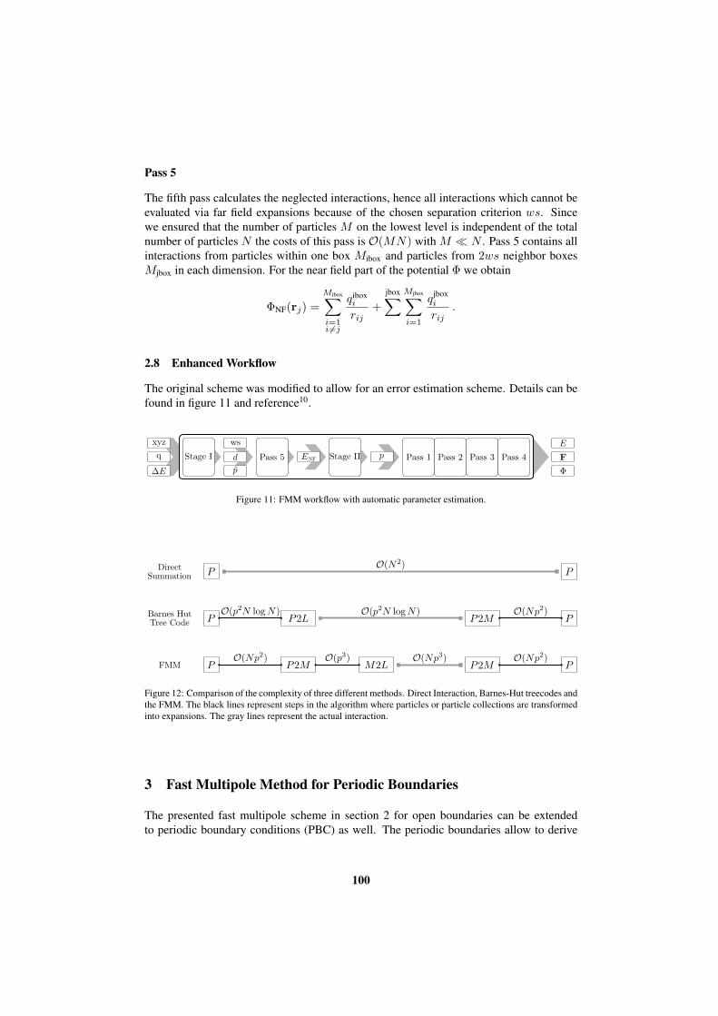
Pass 5
The fifth pass calculates the neglected interactions, hence all interactions which cannot beevaluated via far field expansions because of the chosen separation criterion ws. Sincewe ensured that the number of particles M on the lowest level is independent of the totalnumber of particles N the costs of this pass is O(MN) with M N . Pass 5 contains allinteractions from particles within one box Mibox and particles from 2ws neighbor boxesMjbox in each dimension. For the near field part of the potential Φ we obtain
ΦNF(rj) =
Mibox∑i=1i6=j
qiboxi
rij+
jbox∑Mjbox∑i=1
qjboxi
rij.
2.8 Enhanced Workflow
The original scheme was modified to allow for an error estimation scheme. Details can befound in figure 11 and reference10.
Figure 11: FMM workflow with automatic parameter estimation.
Figure 12: Comparison of the complexity of three different methods. Direct Interaction, Barnes-Hut treecodes andthe FMM. The black lines represent steps in the algorithm where particles or particle collections are transformedinto expansions. The gray lines represent the actual interaction.
3 Fast Multipole Method for Periodic Boundaries
The presented fast multipole scheme in section 2 for open boundaries can be extendedto periodic boundary conditions (PBC) as well. The periodic boundaries allow to derive
100

macroscopic bulk properties of the simulated particle system. A huge (even infinite) en-semble of particles is reduced to a smaller (finite) ensemble inside a finite-sized simulationbox. This simulation box then is replicated in all spatial directions. Hence, the influenceof the boundary on the particles enclosed in the finite simulation box vanishes and only theinfluence of the bulk properties remains. As a particle moves through a boundary into aneighboring image box, it will enter on the opposite site of the central simulation box, thusthe number density is conserved.
To fill the entire 3D space, several different shapes of the central simulation box maybe considered12. However, we only derive the algorithm for the most common shape, i.e.the cubic box. The presented scheme may also be applied together with other shapes likeparallelepipeds, hexagonal prisms, octahedrons or dodecahedrons.
Some simulations even demand a mixed boundary condition with periodic boundariesin only one or two dimensions, such as electrolyte solutions, membranes, nanopores ornanotubes13. The presented FMM scheme can also be applied to such mixed boundarysystems. However, the derivation of the algorithm in this section is performed for threedimensional periodicity if not stated otherwise.
3.1 Definition of the Boundary Condition
The definition of the boundary conditions can be performed in a general manner. We onlyassume that the simulation cell must be translationally symmetric in order to fill the entireRn space. No additional assumptions on the basis vectors forming the periodic lattice arenecessary.
3.2 Three Dimensional Periodicity
We define a simulation cell Γ(0) in three dimensions and the basis vectors a1,a2,a3 with
Γ(0) = r = x1a1 + x2a2 + x3a3 : −1/2 ≤ xi ≤ 1/2, for i = 1, 2, 3 .Additionally, we chose ai in such a way that the volume VΛ of the simulation cell is definedby VΛ = a1 · (a2×a3) > 0. Now, we set up a lattice Λ of translationally symmetric copiesΓ(n) with n = n1a1 + n2a2 + n3a3 and ni ∈ Z of the original central simulation cellΓ(0) by
Γ(n) = r : r− n ∈ Γ(0) .Each replica cell Γ(n) contains the exact same numbers of particles as the simulation cellΓ(0). A particle with position ri in the central simulation cell Γ(0) has a replica particleat ri + n in the lattice cell Γ(n).
For the periodicity in two dimensions and one dimension, we follow the derivation ofthe three dimensional case.
3.3 Convergence of Lattice Sums
Since the potential Φ(R) does not satisfy
|Φ(R)| ≤ A |r|−d−ε (5)
101

Figure 13: (left) The simulation box and its replicas fill the entire space. The space is divided in two regions, anear field region (light gray) and a lattice region (dark gray).
with d being the periodicity and A, ε > 0 for an arbitrary set of point particles with non-zero monopole, dipole- or quadrupole moments, we have to add additional constraints. Thefollowing interactions do not obey the inequality in (5):• Charge–Charge Interactions (1D, 2D, 3D) |r|−1
• Charge–Dipole Interactions (2D, 3D) |r|−2
• Dipole–Dipole Interactions (3D) |r|−3
• Charge–Quadrupole Interactions (3D) |r|−3
Therefore, we add the additional constraint for all particles in the simulation cell
Q =N∑i=1
qi = 0 .
Hence, with box net charge Q = 0 only the dipole terms do not converge absolutely. Weneglect the dipole-dipole contributions temporarily, but will get back to them later.
3.4 Parameter-Free Renormalization Approach
We follow the approach proposed by Kudin and Scuseria14 and incorporate the algorithmlater on into our error control scheme.
The idea for the evaluation of lattice sums with a renormalization approach was firstproposed by Berman and Greengard15. The scheme reduces the infinite summation oflattice sites to a rapidly converging finite summation yielding the lattice operator L. Thepotential Φ(0) at the center of the central box (0, 0, 0) can be computed by adding upcontributions from lattice supercells of size (2ws+ 1)j × (2ws+ 1)j × (2ws+ 1)j withj ∈ N going to infinity. Since we want to translate the multipoles from lattice cells intoTaylor-like (local) expansions around the common center (0, 0, 0) of the central box, wecan add up all contributions into a single translation operator L. We do not add up aninfinite number of lattice sites, however the fast convergence allows to precompute thelattice operator in machine precision. Since the available number of digits is fixed, wecan call a result below machine precision numerically exact and therefore no additionalruntime parameter is introduced.
102

3.4.1 Mathematical Operators
Since this approach is based on the original multipole scheme, we can reuse all introducedFMM translation and conversion operators from section 2. The FMM operators are valid onmultipole moments ωlm and Taylor-like expansions µlm and their chargeless counterpartsOlm and Mlm. For simplicity we only use the chargeless multipole moments Olm andchargeless Taylor-like coefficients Mlm in this section.
3.4.2 Translation of a Multipole Expansion
Let us recall the translation of a multipole expansion Ojk(a) at a to a multipole expansionaround a new center a + b with
Olm(a + b) =l∑
j=0
j∑k=−j
Almjk (b)Ojk(a) .
We are dropping the indices and abbreviate the operator for the following lattice sum algo-rithm via / into the form
O(a + b) = A(b) / O(a) .
3.4.3 Conversion of a Multipole Expansion into a Local Expansion
A multipole expansion at a transforms into a Taylor-like local expansion at b− a via
Mlm(b− a) =
∞∑j=0
j∑k=−j
Blmjk (b)Ojk(a) .
Again, we abbreviate the operator into the form
M(b− a) = B(b)⊗O(a) .
3.4.4 Rescaling of a Multipole Expansion
Since we need a hierarchy of boxes and do not want to recompute multipole moments foreach hierarchy level we introduce a scaling operator for a multipole expansion with
SO(Olm(a)) = 3l ·Olm(a) .
3.4.5 Rescaling of a Local Expansion
For similar reasons, the rescaling has to be performed for the local expansionMlm as well.Therefore, we introduce a scaling operator for a Taylor-like expansion by
SL(Mlm(b)) =Mlm(b)
3l+1.
We limit ourselves to the case where ws = 1. For a larger separation criterion ws, we haveto substitute 3l and 3l+1 with (2ws+ 1)l and (2ws+ 1)l+1 accordingly.
103

3.4.6 Operator Properties
The operators derived in section 2 and the additionally introduced operators SL and SO arelinear operators. Therefore, the following properties apply for infinite expansions
M ⊗ [O1 / O2] = [M ⊗O1]⊗O2
O1 / [O2 / O3] = [O1 / O2] / O3
SL(M)⊗ SO(O) = SL(M ⊗O) (6)
where M represents any Taylor-like local expansion and O represents a certain multipoleexpansion which still gives a convergent expansion when shifted or transformed. Thehierarchy of lattice boxes introduced in the next section guarantees that the speed of con-vergence and precision is not degraded by the use of the operator properties.
3.5 Lattice Sum Algorithm
Let us derive the local moment in the central cell Γ(0) at the center (0, 0, 0) due to anarbitrary lattice cell Γ(n) with n 6= 0 and n = ja1 + ka2 + la3, j, k, l ∈ Z. We define thecontribution with the help of the B operator as
L(j,k,l) = B(n)⊗ ωwith ω being the total multipole moment of the lattice cell. Since all boxes are imagesof the original simulation box at the center, the multipole expansion of each image box isgiven by
ω(n) ≡ ω(0) .
The contribution from all lattice cells for 1D-, 2D- and 3D-periodic systems reads
1D : L∞ =∑
|max(0,0,l)|>1
B((0, 0, l))⊗ ω(a)
2D : L∞ =∑
|max(j,k,0)|>1
B((j, k, 0))⊗ ω(a)
3D : L∞ =∑
|max(j,k,l)|>1
B((j, k, l))⊗ ω(a) .
All nearest neighbors for the central box, i.e. the first layer are excluded to guaranteeconvergence of the expansions. Since the B operator is a linear operator, it allows us toprecalculate B for the entire lattice before applying the unique multipole expansion ω.However, applying a direct space summation like in the last set of equations is difficult,because the convergence of the lattice sum is very slow. But, the evaluation of the latticesum can be rapidly achieved by introducing a hierarchy of supercells with variable size(2ws + 1)j × (2ws + 1)j × (2ws + 1)j . Since we are only interested in the case wherews = 1, we use a hierarchy of size 3j×3j×3j . We define an interaction set as follows. Forthe first interaction set Λ0 we include all lattice cells in the far field of the central (0,0,0)cell but ignore all cells in the near field of the supercell 31×31×31. This rule is equivalentto the partitioning rule in section 2.7 for open boundaries. We write
L∗ =∑Λ0
B((j, k, l)) .
104

The far field contribution from region Λ0 is then
L0 = L∗ ⊗ ω .
We proceed on the next supercell level for j = 1 with cell size 31×31×31. Again we onlyadd cells which are in the near field of the 32 × 32 × 32 supercell. The total contributionto the lattice operator L after this step reads
L1 = L∗ ⊗ ω + SL(L∗)⊗ [O∗ / ω] .
The second contribution demands scaled local moments L∗. At the same time we combinemultipole moments from a 30×30×30 supercell into multipoles of a 31×31×31 supercell.O∗ is defined for each periodic boundary condition by
1D : O∗ =∑
Ω1=−1≤l≤1
A((0, 0, l))
2D : O∗ =∑
Ω1=−1≤j,k≤1
A((j, k, 0))
3D : O∗ =∑
Ω1=−1≤j,k,l≤1
A((j, k, l)) .
Now, we move on to the next level of supercells given by
L2 =L∗ ⊗ ω+ SL(L∗)⊗ [O∗ / ω]
+ SL(SL(L∗))⊗ [SO(O∗) / [O∗ / ω]] .
Applying the operator properties from (6) yield expressions of the form Ln = Ln⊗ω. Weidentify the following partial sums
L0 = L∗
L1 = L∗ + SL(L∗)⊗O∗L2 = L∗ + SL(L∗)⊗O∗ + SL(SL(L∗))⊗ [SO(O∗) / O∗]
= L∗ + SL(L∗ + SL(L∗)⊗O∗)⊗O∗= L∗ + SL(L1)⊗O∗ .
Again, the operator properties allow us to establish an infinite recursion scheme to set upthe lattice sum Ln for increasing n with
L0 = L∗
Ln+1 = SL(Ln)⊗O∗ + L∗ .
The full infinite lattice is defined via the lattice operator
L = L∞ .
Since we want to use the result on a limited precision machine, we halt the recursion aftera certain precision ε has been reached. The convergence of the lattice sum L increaseswith increasing multipole order. Therefore, we have to perform the precision check for the
105

(a) Expand simulation box (gray) to infinity in all periodic dimensions.
(b) Define first interaction set (light gray) and drop near field
(c) Combine multipole expansions
(d) Define second interaction set (light gray)
(e) Size of interaction sets
Figure 14: 1D representation for the computation of the lattice sum. Figure (a) shows the expansion of the(grayed) central simulation box to infinity. Figure (b) shows the dropped nearest neighbors of the simulation boxand the first interaction set. The second interaction set (c)–(d) is generated by combining multipole expansions.Figure (e) shows the increasing size of the interaction sets used with increasing distance to the central simulationcell.
low-order elements. Since, by definition, the monopole element L00 does not converge anddue to symmetry not all elements Llm are non-zero, we halt the recursive scheme when
1D : |Ln+12,0 − Ln2,0| < ε
2D : |Ln+14,0 − Ln4,0| < ε
3D : |Ln+14,0 − Ln4,0| < ε .
The precision goal we used to obtain the unique lattice operator was set to ε = 10−64. Toobtain this precision only 64 iterations are necessary. The lattice constants are independentof the particle distribution and can therefore be precomputed. Since these constants onlydepend on the lattice structure, they have to be recomputed for additional lattice shapes.
106

3.6 Implementation Details
To establish an FMM with periodic boundary conditions we have to add and modify certainparts of the implementation in section 2.7. The error-controlled FMM for open boundariescan be described by the following flow chart:
The periodic FMM needs changes to the scheme. In addition to the original approach wehave to add contributions from the lattice and the first layer around the central box. Thechanges occur in the first stage of the error control, pass 5, the second stage of the errorcontrol and pass 2.
3.7 Additional FMM Pass for the Lattice Operator
Our current implementation uses precomputed values for the lattice operator L in pass2. Since the implementation is based on cubic boxes, currently no other cell shapes areavailable. The extension to different lattice cell shapes demands extra effort for the latticeoperator L. It is possible to precompute L for all required lattices or compute L directly inthe simulation. Therefore, an additional pass has to be added prior to the error control tocompute the missing L terms. The workload of the additional pass is independent of thenumber of particles. It has a complexity of O(p4) with respect to the order of poles p.
3.8 Modifications of FMM Pass 1–5
Pass 1: All multipole expansions have to be shifted to the highest level l = 1. The totalcharge Q of the simulation cell (ω00) has to be zero in order to guarantee convergence.
Pass 2: In addition to the interactions inside the simulation box, far field contributions fromimage boxes have to be taken into account. These interactions will occur on all tree levels.Furthermore, interactions from the lattice with the multipole expansion of the simulationbox have to be calculated.
Pass 3: The computed Taylor-like expansions in pass 2 have to be shifted into the lowestlevel boxes. Since these expansions were generated on all levels, pass 3 translates expan-sions starting at level l = 1.
Pass 4: No changes occur in pass 4. All computed and shifted local moments are combinedwith the multipole moments to yield the far field energy, forces and potentials of the system.
Pass 5: Similarly to pass 2, the near field computation has to take into account interactionsfrom replica particles in image boxes.
107

3.9 Dipole Correction
Until now we neglected the conditionally convergent dipole-dipole interactions. However,since we added the lattice in a spherical manner the element L20 vanishes. A slabwisesummation would yield a different result with L20 6= 0. Unfortunately, the results of sucha periodic FMM computation are still not comparable with a standard Ewald summationscheme at this stage. To compare results we have to transform the obtained extrinsic energyinto an intrinsic energy obtained by an Ewald summation via
Ein = Eex −2π
3d · d
with d =∑i qiai being the dipole moment of the simulation cell. The same correction
has to be applied for the potential
Φin(R) = Φex(R)− 4π
3(R−R0) · d +
2π
3Q
with Q =∑i qiai ·ai being the trace of the Cartesian quadrupole tensor and R0 being the
origin of the coordinate system.
4 Error Control
The implemented Fast Multipole method allows to tune the algorithm specific parameterset on the fly to obtain the optimal computation time for a user-given energy error bound.The corresponding error estimation scheme is very complex and therefore cannot be dis-cussed in the scope of this article. More details on the scheme for open boundaries can befound in reference10 and in an upcoming article for the periodic case.
5 Benchmark
In the following section, we present the scaling of the derived algorithm with respect tothe number of particles N . We use five homogeneously distributed simulation sets. Thesmallest set contains only 4096 particles. Since the computation time for this configurationis around 0.1 seconds, an even smaller test case will not give any additional informationconcerning the scaling. The largest configuration contains about 16 million particles. Allfive sets are used in a computation with mixed or full boundary conditions. The results areillustrated in figure 15. All results were determined on the IBM Power6 JUMP16 cluster atJSC if not stated otherwise.
5.1 Crossover Point with Direct Summation
The crossover point between an FMM and a direct summation can only be specified foropen boundaries, since a direct summation is not possible for the periodic case due tothe infinite number of particles in such systems. For open systems, the crossover point isdetermined at around 500 particles for low precision, i.e. ∆E = 10−3, and 4000 particlesfor high precision calculations, i.e. ∆E = 10−12. The computation time of the errorcontrol scheme is included therein.
108

0.101
0.672
5.38
44
327
103
104
105
106
107
108
Number of Particles
10-1
100
101
102
103
Runti
me
(s)
O (N) Scaling
1D Periodicity
2D Periodicity
3D Periodicity
Open System
(a) Open boundaries
0.101
0.908
8.4
70.9
593
103
104
105
106
107
108
Number of Particles
10-1
100
101
102
103
Runti
me
(s)
O (N) Scaling
2D Periodicity
3D Periodicity
Open System
1D Periodicity
(b) 1D periodic boundaries
0.101
1.14
9.41
75.3
608
103
104
105
106
107
108
Number of Particles
10-1
100
101
102
103
Runti
me
(s)
O (N) Scaling
1D Periodicity
3D Periodicity
Open System
2D Periodicity
(c) 2D periodic boundaries
0.202
1.34
10.4
79
624
103
104
105
106
107
108
Number of Particles
10-1
100
101
102
103
Runti
me
(s)
O (N) Scaling
1D Periodicity
2D Periodicity
Open System
3D Periodicity
(d) 3D periodic boundaries
Figure 15: Scaling of the FMM with open, 1D, 2D and 3D periodic boundary conditions. The solid black linesrepresent the actual periodicity. The remaining shaded lines show, that the impact of the periodic boundary islimited to a factor of two, independent of the number of particles. All results show the optimal O(N) scalingcompared to the reference scaling denoted by a dashed line. When increasing the number of particles for eachplotted point by a factor of eight, the computation time increases roughly by a factor of eight. The difference inthe runtime between open, 1D, 2D and 3D periodic systems originates from the increasing number of boxes atthe boundary of the central box.
5.2 Multi-Billion Particle Testcase
Especially simulations in the field of astrophysics demand huge particle numbers. There-fore, we performed a computation with more than 22 billion particles to check whether theimplementation is capable of dealing with such an amount of data. The test set containedmore than twice the number of particles used in the Millennium simulation17. The com-putation of the energy and forces took 2 days and 16 hours for one time step on a 1.6 GHzItanium CPU with 1 TB of main memory. The precision was set to ∆E = 10−2, whichis sufficient for most astrophysical calculations. This test example shows that this FMMimplementation is capable of computing even very large particle ensembles with limitedresources.
109

10-15
10-12
10-9
10-6
10-3
100
Requested Relative Error ∆E
10-15
10-12
10-9
10-6
10-3
100
FM
M R
elat
ive
Err
or ∆
E
10-12
10-6
100
10-12
10-6
100
Madelung 1D
Madelung 2D
Madelung 3D
Max. Error
Precision 2-52
(a) Energy error bound with double precision
10-30
10-24
10-18
10-12
10-6
100
Requested Relative Error ∆E
10-30
10-24
10-18
10-12
10-6
100
FM
M R
elat
ive
Err
or ∆
E
10-30
10-24
10-18
10-12
10-6
100
10-30
10-24
10-18
10-12
10-6
100
Madelung 1D
Madelung 2D
Madelung 3D
Max. Error
Precision 2-105
(b) Energy error bound with quadruple precision
Figure 16: Precision of FMM calculations with periodic boundary conditions. The requested energy error bounds,pictured as dashed lines in a double precision (a) and quadruple precision (b) computation are never exceeded.The tuning of the optimal parameter set is done automatically. Due to symmetry the achieved energy error boundfor 3D periodic systems is slightly higher compared to 2D or 1D systems.
5.3 Precision Verification
The precision of calculations with periodic boundaries can be verified directly against an-alytically known or rapidly converging solutions. That is, a Madelung particle system18
serves as reference system. The Madelung constant characterizes the potential Φ at theorigin due to the periodic lattice. The reference energy is determined by adding up allcontributions 1
2
∑Ni=1 qiΦ(ri) inside the simulation box. The size of the simulation box
for any periodicity can be increased by adding more and more particles from replica boxes.Thereby, it is possible to verify the precision of the algorithm even for millions of particles.All precision checks are performed for several simulation box sizes up to approximately16 million particles. The results do not show any additional errors with increasing systemsize, except for minor fluctuations at machine precision for 88 particles. The data plottedin figure 16 is taken from test runs with the smallest possible Madelung particle sets.
5.4 Precision Scaling
The FMM allows optimal computation time for low as well as high precision simulations.Depending on the user-requested energy error bound the computation time will increaseor decrease. As depicted in figure 17a the FMM computes a system with an error boundof 10−1 nine times faster compared to a high precision error bound of 10−15. Since theerror estimation scheme can be regarded as a FMM itself the computation time for lowprecision 10−1 includes a large amount of tuning time contributing 49.9%. Since thistuning overhead is almost constant for a given particle system, hence independent of therequested precision, the percentage will decrease with increasing precision. To obtain aneven faster computation for low precision simulations, the error estimation can be disabledfor several time steps.
110

10-1
10-3
10-5
10-7
10-9
10-11
10-13
10-15
Requested Relative Energy Error ∆E
20
60
100
140
180
Tim
e (s
)
∆0 = 0 ∆
1 = 5.48 ∆
2 = -1.97[log
10(∆E)]
0.97
(a) Computation time with decreasing error bound
10-1
10-3
10-5
10-7
10-9
10-11
10-13
10-15
Requested Relative Energy Error ∆E
0
10
20
30
40
50
Err
or
Est
imat
ion T
ime
[%]
10.2%
1.0%
(b) Error estimation time with decreasing error bound
Figure 17: The computation time for 2097152 particles (including the time to tune the FMM parameter) isdepicted in (a). The graph can be divided in three sections. A low precision section (10−1 . . . 10−4), where thecomputation time is constant (∆0). A section (10−4 . . . 10−9) where the computation time increases linearly(∆1). And a high precision section (∆2) where the computation time follows a power law. The percentage ofcomputation time of the error estimation scheme is shown in (b). The tuning can be disabled for several time stepsduring a simulation, since a (small) number of time steps most likely won’t change the optimal FMM parameterset.
Parallel Scaling And Efficiency
The FMM shows almost ideal scaling for homogeneously distributed particle systems. Fora system consisting of 2097152 particles and open boundary conditions a strong scalingtest (see figure 18a) was performed up to 64 processors. The computation time with 64processors was 0.24 seconds. The parallel efficiency at 64 processors achieved 95.6%. Asecond example with one billion particles is shown in figure 18b. The parallel efficiency at256 processors is 95.2% and the runtime 34.5 seconds. The improvement at 16 processorswas due to memory consumption. Using less than 16 processors resulted in non-localmemory access across a SMP node and therefore slowed down the computation.
6 Main Features
The main features of the current FMM implementation can be summarized as follows• allows the computation of energy, potential and forces,• comes with full energy error control,• includes a on-the-fly runtime minimization,• can handle open, 1D, 2D and 3D periodic boundary conditions,• computes 50k – 150k particles per second and core,• has a small memory footprint,• is available in single/double/quadruple precision,• allows exchangeable cusp potential in the near field,• can handle homogeneous and clustered particle systems,• is available on Intel/Linux, IBM Power6/AIX, BlueGeneP, HP/Linux machines.
111

1 2 4 8 16 32 64Number of Processors
1
2
4
8
16
32
64
Sca
lin
g
(a) Scaling with 2097152 particles
1 2 4 8 16 32 64 128 256Number of Processors
1
2
4
8
16
32
64
128
256
512
Sca
lin
g
(b) Scaling with 1073741824 particles
Figure 18: Strong scaling for two homogeneously distributed particles systems on JUMP16.
7 Summary
We described an O(N) implementation of the Fast Multipole Method for open and peri-odic boundary conditions in one, two and three dimensions. The attached error estimationscheme was verified for several precisions with one-, two- and three-dimensional period-icity and revealed tight error bounds never exceeding the requested threshold.
Finally, we can conclude that the presented FMM implementation provides an idealCoulomb solver for open and periodic boundary conditions. The scientific communitymay benefit from this implementation, since algorithmic details, like tuning the FMM pa-rameters are hidden from the user and will be adjusted automatically without affectingthe computation time. Even high precision calculations up to machine precision can beperformed without degrading the runtime. Furthermore, the developed FMM library isindependent of third-party libraries and has a small memory footprint.
The developed code provides a firm framework for simulations in the field of moleculardynamics and astrophysics. It is well tested with real world examples and is used in aproduction environment at Max Planck Institute for the Physics of Complex Systems inDresden19–22.
References
1. O. D. Kellogg, Foundations of Potential Theory, Springer, 1967.2. I. Gradshteyn and I. W. Ryzhik, Tables of Integrals, Series and Products , Academic
Press, 1965.3. C. A. White and M. Head-Gordon, Derivation and efficient implementation of the fast
multipole method, J. Chem. Phys., 101, 6593–6605, 1994.4. M. J. Caola, Solid harmonics and their addition theorems, J. Phys. A Math. Gen., 11,
2, L23-L25, 1978.5. J. Choi, Notes on formal manipulations of double series, Commun. Korean Math.
Soc., 18, 4, 781–789, 2003.
112

6. J. Barnes and P. Hut, A hierarchical O(N log N) force-calculation algorithm, Nature,324, 446–449, 1986.
7. C. A. White and M. Head-Gordon, Rotating around the quartic angular momentumbarrier in fast multipole method calculations, J. Chem. Phys., 105, 12, 5061–5067,1996.
8. L. Greengard and V. Rokhlin, A fast algorithm for particle simulations, J. Comput.Phys., 73, 2, 1987, 325–348.
9. L. Greengard and V. Rokhlin, A new version of the Fast Multipole Method for theLaplace equation in three dimensions, Acta Numer., 6, 229–269, 1997.
10. H. Dachsel, An error-controlled fast multipole method, J. Chem. Phys., 132, 11,119901, 2010.
11. H. Dachsel and M. Hofmann and G. Runger, Library Support for Parallel Sorting inScientific Computations, Euro-Par 2007 Parallel Processing, 695–704, 2007.
12. H. S. M. Coxeter, Regular Polytopes, Dover Publications, 1973.13. A. Leach, Molecular Modelling: Principles and Applications (2nd Edition), Prentice
Hall, 2001.14. K. N. Kudin and G. E. Scuseria, Revisiting infinite lattice sums with the periodic fast
multipole method, J. Chem. Phys., 121, 7, 2886–2890, 2004.15. C. L. Berman and L. Greengard, A renormalization method for the evaluation of lat-
tice sums, J. Math. Phys., 35, 11, 6036–6048, 1994.16. http://www2.fz-juelich.de/jsc/jump17. V. Springel et al., Simulating the joint evolution of quasars, galaxies and their large-
scale distribution, Nature, 435, 629, 2005.18. R. E. Crandall and J. F. Delord, The potential within a crystal lattice, J. Phys. A Math.
Gen., 20, 9, 2279, 1987.19. A. Mikaberidze and U. Saalmann, and J. M. Rost, Laser-Driven Nanoplasmas in
Doped Helium Droplets: Local Ignition and Anisotropic Growth, Phys. Rev. Lett.,102, 12, 128102, 2009.
20. U. Saalmann, Electron emission from laser-irradiated atomic clusters, Laser Phys.,19, 2, 202–207, 2009.
21. C. Gnodtke, and U. Saalmann, and J. M. Rost, Ionization and charge migrationthrough strong internal fields in clusters exposed to intense x-ray pulses, Phys. Rev.A, 79, 4, 041201, 2009.
22. G. Bannasch and T. Pohl, Formation of Atoms in Strongly Correlated, Ultracold Plas-mas, MPIPKS Technical Report, 2008.
113


Multigrid Methods for Long-Range Interactions
Matthias Bolten
Fachbereich Mathematik und NaturwissenschaftenBergische Universitat Wuppertal
42097 Wuppertal, GermanyE-mail: [email protected]
Multigrid methods are optimal methods for the solution of certain PDEs and therefore widelyused in different simulation codes in science and engineering. Starting from the formula forcalculating the electrostatic potential we derive a formulation of this and related problems thatallows for the application of multigrid methods in the calculation of these long-range interac-tions. The resulting methods are optimal, if the particles are almost evenly distributed and canbe parallelized in a very efficient way.
1 Introduction
Electrostatic and gravitational interactions are long-ranged interactions that are importantfor many applications in e.g. biophysics or astrophysics. Due to their close relation to thePoisson equation
−∆u(x) = f(x), for x ∈ Ω,
for a suitable domain Ω and appropriate boundary conditions, these interactions can beequivalently treated by the solution of this elliptic partial differential equation (PDE) witha certain right hand side. Under the assumption that the particles are evenly distributed orat least only mildly clustered, numerical methods can be designed that are optimal, if thesolution of the partial differential equation is available.
The numerical solution of the Poisson equation is well studied as it is the prototypeof an elliptic PDE, in fact it serves as a model problem in most textbooks on numericalsolution of PDEs, and it is needed in different fields. As a consequence fast numericalmethods have been developed, fast Poisson solvers include specialized direct methods likethe cyclic reduction method or FFT-based techniques, as well as iterative methods likeSOR, the CG method or multigrid methods. While the first are specifically tailored to thematrices arising while using a special discretization, the latter often suffer from the factthat the number of iterations necessary to solve the system up to a given accuracy growswith the system size. This is not the case for multigrid methods, which yield a solution upto discretization accuracy in optimal, i.e. O(N), complexity.
The combination of the approach using the solution of the Poisson equation outlinedabove combined with an efficient multigrid method yields an optimal method for the com-putation of energies and forces due to electrostatic and gravitational interactions.
In the following, we will first introduce multigrid methods in general in Section 2.In Section 3 the application of multigrid methods in methods involving electrostatic andgravitational interactions is discussed in detail. For that purpose the relation between 1/r-potentials and the Poisson equation is presented in Section 3.1, then the basic numericalmethod is derived in Section 3.2 and finally the relevant boundary conditions are treated
115

in Section 3.4 and Section 3.3. The parallelization of the method is described in Section 4and a conclusion is drawn in Section 5.
2 Multigrid Methods
The development of multigrid methods goes back at least to the works of Fedorenko1 andBakhvalov2. Later the work of Brandt3 unleashed the full potential of multigrid methods.The following introduction is very brief, so we omit proofs, and focussed onto the case ofthe Poisson equation. An introduction that goes beyond the following can be found in thework of Briggs et al.4, the book of Trottenberg et al.5 contains the theoretical foundationof multigrid methods as well as descriptions of advanced multigrid techniques.
2.1 Motivation
As motivation we consider the following Poisson equation
−∆u(x) = f(x), for x ∈ Ω andu(x) = 0 for x ∈ ∂Ω,
where Ω = [0, 1]2. This can be discretized on a rectangular grid withN = (n+1) ·(n+1)grid points using the standard 5-point scheme, yielding the linear system of equations ofthe form
1
h2(4ui,j − ui−1,j − ui+1,j − ui,j−1 − ui,j+1) = fi,j , for i, j = 1, . . . , nk,
where h = 1/n and ui,j = 0 for i ∈ 0, n + 1 or j ∈ 0, n + 1. For the sake ofsimplicity, in the following we write the vectors u, f etc. with two indices, where necessary,to emphasize that they represent quantities on the grid. An actual implementation also oftenuses a two-dimensional field for each of these vectors.
The resulting linear system is denoted by
Lu = f, (1)
where L ∈ RN×N and u, f ∈ RN . One easily verifies that the eigenvalues λl,m andeigenvectors ϕl,m of the system matrix L are given by
λl,m = 4− 2 cos(lπh)− 2 cos(mπh), (2)(ϕl,m)i,j = sin(lπih) sin(mπjh), (3)
for l,m = 1, . . . , n. The system can be solved using a simple iterative method, e.g. withthe Jacobi method.Definition 2.1 (Jacobi method). Let A ∈ RN×N , let b ∈ RN and let the solution x ∈ R ofthe linear system
Ax = b
be sought for. Let D ∈ RN×N be a diagonal matrix containing the main diagonal of A.Then the Jacobi method is defined as
φJacobi : RN × RN → RN
(x(k), b) 7→ φJacobi(x(k), b) = x(k+1),
116

where
x(k+1) = x(k) −D−1(Ax(k) + b), k = 1, 2, . . . ,
and x(0) is an initial guess. The iteration matrix is given by MJacobi = −D−1(D −A).The following theorem states a sufficient condition for the convergence Jacobi method:
Theorem 2.2. Let both A be symmetric positive definite and let the relation
2D > A > 0
hold. Then the Jacobi method converges and its convergence rate is given by
ρ(MJacobi) = ‖MJacobi‖A = ‖MJacobi‖D < 1.
With the help of this theorem and the observation that the smallest of the eigenvaluesof L given by (2) is
λmin = 4(1− cos(πh))
we obtain that
ρ(MJacobi) = cos(πh),
so the Jacobi method converges slowly for larger systems, i.e. smaller h. Examination ofthe error
e(k) = u∗ − u(k),
where u∗ = L−1. With the help of the iteration matrix MJacobi we obtain that the eigenvec-tor ϕl,m is damped by a factor of | 12 (cos(lπh) cos(mπh))|, so error components co-linearto eigenvectors with indices l,m in the middle of 1, . . . , n are damped efficiently, whilecomponents co-linear to eigenvectors with large or small indices are not damped efficiently.By introducing a relaxation parameter ω we obtain the JOR method given by the followingdefinition:Definition 2.3 (Jacobi method). Under the same assumptions as in Definition 2.1 the JORmethod is defined as
φJOR : RN × RN → RN
(x(k), b) 7→ φJOR(x(k), b) = x(k+1),
where
x(k+1) = x(k) − ωD−1(Ax(k) + b), k = 1, 2, . . . ,
and x(0) is an initial guess. The iteration matrix is given by MJOR,ω = −ωD−1(D −A).Similar to Theorem 2.2 one obtains:
Theorem 2.4. Let A ∈ RN×N be symmetric and and positive definite and let ω fulfill
0 < ω < 2/ρ(D−1A).
Then the JOR method converges, and its convergence rate is given by
ρ(MJOR,ω) = ‖MJOR,ω‖A = ‖MJOR,ω‖D < 1.
117

00.5
1
00.5
1
0.20.40.60.81
00.5
1
00.5
1
0.20.40.60.81
00.5
1
00.5
1
0.20.40.60.81
Figure 1: Error of an arbitrarily chosen initial approximation and right hand side of the Laplacian discretized onthe unit square using 152 grid points before and after application of one and three iterations of a damped Jacobimethod with ω = 4/5.
So we obtain that error components co-linear to the eigenvector ϕl,m are damped by afactor of |1− ω
2 (2− cos(lπhk)− cos(mπhk))|. Now, by choosing ω appropriately, errorcomponents that are co-linear to λl,m with l and m close to n can also be reduced, but thebehavior for components corresponding to l,m almost 0 is not changed. This behavior canbe observed in Figure 1: Obviously, the error components that belong to highly oscillatingparts of the error are reduced efficiently, while components that vary slowly are merelyaffected at all. This is one important observation for the derivation of multigrid methods.The other observation is that a slowly varying error can be represented on a coarser grid.
2.2 Two-grid methods
Guided by the ideas of the previous section, we will now derive two-grid methods. For thatpurpose, we assume that the system to solve is such that n = n` = 2` − 1 for some ` ∈ N.Consequently we denote the associated system matrix by L` and the grid spacing by h`.The right hand side, current approximation to the solution etc. also are added an ` to denotethat they belong to this level. Next, another, coarser level ` − 1 with n`−1 = 2`−1 − 1 isintroduced. To define a two-grid method we now need three ingredients:
1. smoother
2. grid-transfer operators
3. coarse-grid correction operator
2.2.1 Smoother
Due to the above observation, iterative methods like the Jacobi method are called smoothersin the multigrid setting. For the analysis of the smoother we first define low and highfrequencies:Definition 2.5. Let L be given by (1). The eigenvector ϕ`;l,m as given by (3) is called
low frequency, if max(l,m) < (n` + 1)/2,
high frequency, if (n` + 1)/2 ≤ max(l,m).
Now, the smoothing factor of the JOR method is defined as the worst factor by whicha high frequency is damped:
118

0 0.2 0.4 0.6 0.8 1!1
!0.5
0
0.5
1
low frequencies
high frequencies
frequency
dam
ping
! = 1! = 1/2! = 2/3
Figure 2: Damping factors χl,m for h → 0 of the JOR method for the 1D analogon to our model problem fordifferent relaxation parameters ω. The choice ω = 2/3 is optimal and all high frequency components are dampedby a factor of at least 1/3.
Definition 2.6. Let L be given by (1) and let
χ`,l,m(ω) := 1− ω
2(2− cos(lπh`)− cos(mπh`))
be the factor by which the eigenvector ϕ`;l,m is damped by the JOR method. Then thesmoothing factor µ(ω) of the JOR method is defined as
µ`(ω) := max|χ`;l,m(ω)| : (n` + 1)/2 ≤ max(l,m) ≤ n`,
Further:
µ(ω) = sup`∈N
µ`(ω).
Thus the relaxation parameter is optimal if ω as the minimizer of µ(ω). In the 2D caseω = 4/5 is optimal. For the 1D analogon of our problem the choice ω = 2/3 is optimal,as depicted in Figure 2.
2.2.2 Grid-transfer operators
For the transfer from the fine level ` to the coarse level `− 1 and vice versa restriction andprolongation operators are needed. An example for a restriction operator, that is widelyused and that is used in our examples is the full-weighting operator. This operator justdoes an averaging over neighboring components on the grid.Definition 2.7. The full-weighting operator I`−1
` transfers a quantity v` from level ` tolevel `− 1 by
(v` − 1)i,j = I`−1` v`
=1
16(4(v`)2i,2j + 2(v`)2i−1,2j + 2(v`)2i+1,2j + 2(v`)2i,2j−1 + 2(v`)2i,2j+1+
(v`)2i−1,2j−1 + (v`)2i−1,2j+1 + (v`)2i+1,2j−1(v`)2i+1,2j+1),
119

for i, j = 1, . . . , n`−1. An alternative description is the stencil
1
16
1 2 12 4 21 2 1
`−1
`
As we deal with zero Dirichlet boundary conditions in our model problem, the valueson the boundaries of the grid are always defined to vanish. For prolongation, bilinearinterpolation is widely used.Definition 2.8. The bilinear interpolation operator transfers a quantity v`−1 from level`− 1 to level ` by
(v`)i,j = I``−1v`−1
=1
4
4(v`−1)i/2,j/2, for i even and j even,2((v`−1)(i−1)/2,j/2 + (v`−1)(i+1)/2,j/2), for i odd and j even,2((v`−1)i/2,(j−1)/2 + (v`−1)(i/2,(j+1)/2), for i even and j odd,(v`−1)(i−1)/2,(j−1)/2 + (v`−1)((i+1)/2,(j+1)/2+
(v`−1)(i−1)/2,(j−1)/2 + (v`−1)((i+1)/2,(j+1)/2, for i odd and j odd,
for i, j = 1, . . . , n`. Alternatively, it is described by the stencil
1
4
1 2 12 4 21 2 1
``−1
.
Note that the brackets around the stencil of prolongation operator are interchanged torepresent that using this stencil means giving values to another quantity. The extension ofthese operators to 3D is straightforward.
2.2.3 Coarse grid correction operator
Using the restriction and prolongation operators, as well as a discretization of the problemon level ` − 1, the coarse grid operator can be defined. For that purpose, we examine theresidual
r(k)` = f` − L`u(k)
`
for some approximative solution x(k)` . The residual is the solution of the system
L`rk` = ek` ,
where e(k)` = L−1
` f`−x(k)` is the error. If the error consists is dominated by low-frequency
modes, it is well approximated on the coarser grid, i.e. by e(k)` ≈ I``−1e
(k)`−1. Similarly, for
the residual we have r(k)`−1 ≈ I`−1
` r(k)` , combining this with the operator on the coarser
level yields
e(k)` ≈ I``−1L
−1I`−1` r
(k)` ,
120
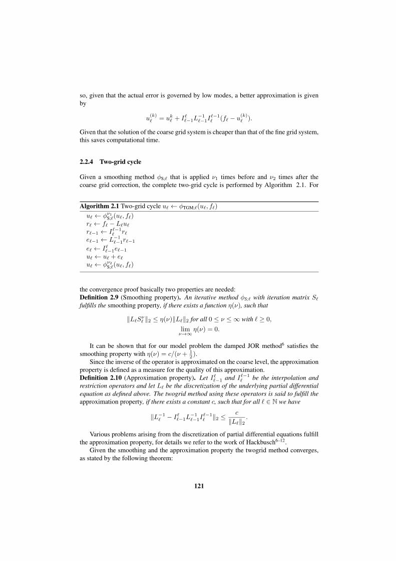
so, given that the actual error is governed by low modes, a better approximation is givenby
u(k)` = uk` + I``−1L
−1`−1I
`−1` (f` − u(k)
` ).
Given that the solution of the coarse grid system is cheaper than that of the fine grid system,this saves computational time.
2.2.4 Two-grid cycle
Given a smoothing method φS;` that is applied ν1 times before and ν2 times after thecoarse grid correction, the complete two-grid cycle is performed by Algorithm 2.1. For
Algorithm 2.1 Two-grid cycle u` ← φTGM;`(u`, f`)
u` ← φν1S;`(u`, f`)r` ← f` − L`u`r`−1 ← I`−1
` r`e`−1 ← L−1
`−1r`−1
e` ← I``−1e`−1
u` ← u` + e`u` ← φν2S;`(u`, f`)
the convergence proof basically two properties are needed:Definition 2.9 (Smoothing property). An iterative method φS;` with iteration matrix S`fulfills the smoothing property, if there exists a function η(ν), such that
‖L`Sν` ‖2 ≤ η(ν)‖L`‖2 for all 0 ≤ ν ≤ ∞ with ` ≥ 0,
limν→∞
η(ν) = 0.
It can be shown that for our model problem the damped JOR method6 satisfies thesmoothing property with η(ν) = c/(ν + 1
2 ).Since the inverse of the operator is approximated on the coarse level, the approximation
property is defined as a measure for the quality of this approximation.Definition 2.10 (Approximation property). Let I``−1 and I`−1
` be the interpolation andrestriction operators and let L` be the discretization of the underlying partial differentialequation as defined above. The twogrid method using these operators is said to fulfill theapproximation property, if there exists a constant c, such that for all ` ∈ N we have
‖L−1` − I``−1L
−1`−1I
`−1` ‖2 ≤
c
‖L`‖2.
Various problems arising from the discretization of partial differential equations fulfillthe approximation property, for details we refer to the work of Hackbusch6–12.
Given the smoothing and the approximation property the twogrid method converges,as stated by the following theorem:
121
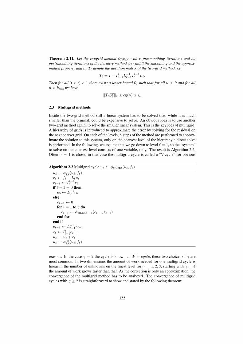
Theorem 2.11. Let the twogrid method φTGM;` with ν presmoothing iterations and nopostsmoothing iterations of the iterative method φS;` fulfill the smoothing and the approxi-mation property and by T` denote the iteration matrix of the two-grid method, i.e.
T` = I − I``−1L−1`−1I
`−1` L`.
Then for all 0 < ζ < 1 there exists a lower bound ν, such that for all ν > ν and for allh < hmax we have
‖T`Sν` ‖2 ≤ cη(ν) ≤ ζ.
2.3 Multigrid methods
Inside the two-grid method still a linear system has to be solved that, while it is muchsmaller than the original, could be expensive to solve. An obvious idea is to use anothertwo-grid method again, to solve the smaller linear system. This is the key idea of multigrid:A hierarchy of grids is introduced to approximate the error by solving for the residual onthe next coarser grid. On each of the levels, γ steps of the method are performed to approx-imate the solution to this system, only on the coarsest level of the hierarchy a direct solveis performed. In the following, we assume that we go down to level ` = 1, so the “system”to solve on the coarsest level consists of one variable, only. The result is Algorithm 2.2.Often γ = 1 is chose, in that case the multigrid cycle is called a “V-cycle” for obvious
Algorithm 2.2 Multigrid cycle u` ← φMGM;`(u`, f`)
u` ← φν1S;`(u`, f`)r` ← f` − L`u`r`−1 ← I`−1
` r`if `− 1 = 0 thene0 ← L−1
0 r0
elsee`−1 ← 0for i = 1 to γ doe`−1 ← φMGM;`− 1(e`−1, r`−1)
end forend ife`−1 ← L−1
`−1r`−1
e` ← I``−1e`−1
u` ← u` + e`u` ← φν2S;`(u`, f`)
reasons. In the case γ = 2 the cycle is known as W − cycle, these two choices of γ aremost common. In two dimensions the amount of work needed for one multigrid cycle islinear in the number of unknowns on the finest level for γ = 1, 2, 3, starting with γ = 4the amount of work grows faster than that. As the correction is only an approximation, theconvergence of the multigrid method has to be analyzed. The convergence of multigridcycles with γ ≥ 2 is straightforward to show and stated by the following theorem:
122

Theorem 2.12. With the same notation as above let
‖Sν2` T`Sν1` ‖∗ ≤ σ, ‖Sν2` I``−1‖∗‖L−1`−1I
`−1` L`S
ν1k ‖∗ ≤ c
hold uniformly for all levels ` for some norm ‖ ·‖∗. Then the ∗-norm of the iteration matrixMk is bounded by η`, where η` is defined recursively as
η0 = σ, ηk = σ + cηγk−1 (k = 1, 2, . . . ),
where c, σ > 0. For γ = 2 and
4cσ ≤ 1
the ∗-norm of the iteration matrix M` is bounded from above by
‖M`‖∗ ≤ η =1
2c(1−
√1− 4cσ) ≤ 2σ,
so for σ < 12 the method converges with a uniformly bounded convergence rate.
As a consequence, multigrid methods are optimal methods in the sense that the conver-gence rate is bounded independently of the level and that one iteration of the method haslinear computational cost.
2.4 Advanced multigrid techniques
While this brief introduction is relatively easily extendible to other elliptic PDEs, other do-mains, including more complex ones, and other boundary conditions, e.g. periodic bound-ary conditions, the development of multigrid methods goes much further than that. Multi-grid methods have been developed for non-elliptic problems and for non-linear problems.Further on algebraic multigrid methods (AMG) allow the use of this idea without the ex-plicit generation of the grid hierarchy, this is important e.g. when multigrid has to be usedas a black box solver in a mature code. These developments go far beyond the scope ofour introduction, a good overview and introduction into more advanced multigrid methodsis given in the book of Trottenberg et al.5.
3 Multigrid Methods for Long-Range Interactions
As just shown multigrid methods are optimal solvers for the Poisson equation. In the intro-duction we noted that the use of an optimal Poisson solver leads to an optimal method for1/r-potentials. In the following, we will derive the numerical method. The idea is relatedto that of the P3M method that is described e.g. in the book of Hockney and Eastwood13.In contrast to the P3M we start deriving the method for the open space problem.
3.1 Electrostatic interactions and the Poisson equation
Assume that the electrostatic energy of a system ofN particlesa with charges qi at positionsxi, i = 1, . . . , N has to be calculated, i.e. the sum
E =1
2
N∑i=1
qi
N∑j=1,j 6=i
1
4πε0
qj‖xi − xj‖2
.
aNote that this N is different from the one in the previous chapter.
123

Obviously, the electrostatic potential Ui of particle i is given by the part inside of the outersum, so
Ui = qi
N∑j=1,j 6=i
1
4πε0
qj‖xi − xj‖2
.
As the Green function of the 3D Laplace operator isG(x) = 1/(4π‖x‖2) this is equivalentto the solution Φ of the Poisson equation
−∆Φi(x) =1
ε0
N∑j=1,j 6=i
qjδ(‖x− xj‖2)
evaluated at the position xi. As the right hand side consists of a superposition of δ-distributions, this equation cannot be solved numerically. To make it accessible by nu-merical methods, we replace the δ-distributions on the right hand side by a functionρg = g(‖x‖2). We choose the function g : R+
0 → R+0 such that g is sufficiently smooth,
such that ∫R3
ρg(x)dx = 1
and such that the solution Φg of the Poisson equation
−∆Φg(x) =1
ε0ρg(x)
is known analytically. This is similar to the introduction of the error function in the Ewaldsummation, in contrast to this additionally we demand that g has limited support R > 0.So the potential of particle i is given as
Ui = qi
Φi(xi)−∑
j∈Mi\i
qjΦg(xi − xj)−1
4πε0
qj‖xi − xj‖2
, (4)
where Φi is the solution of the Poisson equation
−∆Φi(x) =1
ε0
N∑j=1,j 6=i
qjρg(‖x− xj‖2)
and where Mi = j : ‖xj − xi‖2 < R denotes the set of all indices j ∈ 1, . . . , Nthat closer to particle i than the support of g, including i. This sum is a simple near-fieldcorrection.
Now, by subtracting the self-energy correction term qiΦg(0) from (4), we obtain
Ui = qi
Φi(xi)−∑j∈Mi
qjΦg(xi − xj)−1
4πε0
1j‖xi − xj‖2
and we can replace the Φi, i = 1, . . . , N by Φ, the solution of the single Poisson equation
−∆Φ(x) =1
ε0
N∑j=1
qjρg(‖x− xj‖2) (5)
124

and the energy is given by
E =1
2
N∑i=1
Ui.
We like to note that no additional errors have been introduced by this transformation. Inmolecular dynamics simulations not the energy, but the forces are of interest. Obviouslythe force acting on particle i is given by
Fi = qi∇Φ(xi) + near-field correction.
A self-energy correction is not necessary, here.
3.2 Basic numerical method
With the previous chapter, a numerical method can be derived easily. For finding the neigh-bors that are necessary in the near-field correction, the linked-cell algorithm is used, as itis described in the book of Hockney and Eastwood13. Here we assume that a cell spacingh is used. The initialization of the necessary data structures is given by Algorithm 3.1. Tokeep the algorithm simpler by bold indices we denote multi-indices.
Algorithm 3.1 Linked-list initializationfor i ∈ G do
HOC(i)← 0end forfor i = 1 to N do
j← round(x/h)LL(i)← HOC(j)HOC(j)← i
end for
The data structure initialized by this algorithm is used in the basic numerical method.Further on the method uses the solution of the Poisson equation (5) on a mesh, for easeof implementation that mesh can coincide with the mesh introduced due to the linked-listdata structure. Finally, the basic method is given by Algorithm 3.2.
At this point, given that the numerical solution of is exactly available on the grid, theonly error in the method is due to the interpolation of the potential surface.
3.3 Open boundary conditions
In the open boundary case the Poisson equation (5) has to be solved with boundary condi-tions
Φ(x)→ 0, as ‖x‖2 →∞.Multigrid methods are well-suited for the numerical solution of this problem. The basicidea is to extend and coarsen the grid successively and impose Dirichlet boundary condi-tions with the help of the Green function on the coarsest level. This scheme is depicted in
125

Algorithm 3.2 Basic numerical methodfor i ∈ G do
for j ∈ j : ‖i− j‖∞ ≤ R/h dok = HOC(j)while k 6= 0 dof(xi) = qkρga(xi − xk)k = LL(k)
end whileend for
end forSolve ∆Φga,P = f numerically using Poisson solverE = 0for k = 1, . . . , N do
Approximate Φga,P(xk) by interpolating the potential surfaceE = E + qk(Φga,P(xk)− Φga(0))for j ∈ j : ‖round(xk/h)− j‖∞ ≤ R/h dok = HOC(j)while k 6= 0 doE = E − qkΦ(xi − xk) + 1
4πε0
qiqk‖xi−xk‖2
k = LL(k)end while
end forend for
Figure 3: Coarsened grid in 2D.
2D in Figure 3. It can be shown that the error of the numerical method is of the requiredorder and that the numerical complexity stays linear. The details are beyond the scope of
126

Pi,jPi-1,j Pi+1,j
Pi,j-1
Pi,j+1
Figure 4: Domain splitting in the 2D case. Highlighted is the part of the domain for which processor Pi,j isresponsible, the part that is highlighted lighter is the ghost area.
this introduction, for details we refer to the work of the author14, 15.
3.4 Periodic boundary conditions
For periodic boundary conditions (5) has to be solved on the torus R3/Z3, so the settingof explicit boundary conditions is not necessary. The basic numerical method given byAlgorithm 3.2 needs only slight modifications, namely in the linked list data structure ithas to be taken into account that the periodic images exist.
In contrast to the simple multigrid method described above, to simplify implementationthe grid sizes should be chosen such that on level ` the grid has n` = 2` grid points. Thefull-weighting operator given by Definition 2.7 and the linear operation operator given byDefinition 2.8 are then easily adopted to take into account the grid points in the periodicimages. Not that the linear system is singular with the constant vector, i.e. the vectorconsisting of ones, only, in the kernel.
4 Parallelization
The resulting method can be parallelized efficiently with the help of a standard domainsplitting schemeb, i.e. the physical domain is distributed onto the available processors.This situation is depicted for the 2D case in Figure 4. The physical domain Ω is mappedonto a threedimensional processor grid, such that processor Pi,j,k contains subdomainΩi,j,k, where⋃
i,jk
Ωi,j,k = Ω, Ωi,j,k ∩ Ωi′,j′,k′ = ∅ for i 6= i′, j 6= j′, k 6= k′.
On each processor the domain is enlarged by a ghost area, such that the necessary data isavailable during computation. The ghost area for the multigrid method contains the grid
bThe term domain splitting is used here to distinguish this data distribution scheme from the numerical methodthat is called domain decomposition.
127

1e-05
1e-04
0.001
0.01
0.1
1
10
100 1000 10000
t [s]
# processors
init linked list and copy ghostsassign charges
init solver variablessolve
interpolatecorrect near-field
total
Figure 5: Timings for 2097152 particles on a 128 × 128 × 128 grid on the Blue Gene/P system JUGENE inJulich.
points needed to calculate the local matrix-vector product and to interpolate and restrict thedata. The ghost area for the particle part of the method has to contain the particles locatedin the ghost area, the necessary data structures, i.e. the linked list entries, and the meshedsolution of the PDE. These ghost areas do not have to be the same and they are updatedwhenever it is needed, i.e. the particles in the ghost area have to be exchanged at the be-ginning of the computation and the solution of the PDE has to be updated after it has beencomputed in the particle part of the method, in the multigrid method an update is neces-sary after each smoothing step and after applying restriction and interpolation. Using thisparallelization scheme, parallelization of the basic numerical method is straightforward.
The parallelization of multigrid methods needs more attention. As the problem size isreduced on the coarser grids, at some point there are fewer variables, than processors todistribute the work to. There are basically two options to deal with this situation. First,it is possible to let the processors that are not assigned a variable stay idle during thecomputation on these coarser levels. The second option is to stop coarsening on this leveland to solve the system directly on this level. The second option needs a parallel directsolver, while the first introduces a load-imbalance. As in practice the problems on theselevels are relatively small compared to the finer levels, the first option is in many cases adecent choice. An overview over parallelization approaches for multigrid methods can befound in the survey paper of Chow et al.16.
Our implementation of a multigrid-based method for the calculation of electrostaticinteractions is based on the described 3D-domain splitting approach with idle processorson the coarser grids of the multigrid hierarchy. The timings of the different steps can befound in Figure 5. The method has been implemented using C99 and FORTRAN and thetiming results are obtained for 2097152 particles on a 128 × 128 × 128 grid on the BlueGene/P system JUGENE in Julich. The speedup and efficiency plots for this test can be
128

100
1000
10000
100 1000 10000
spee
dup
# processors
0.65
0.7
0.75
0.8
0.85
0.9
0.95
1
100 1000 10000
effic
ienc
y
# processors
Figure 6: Speedup and efficiency for 2097152 particles on a 128 × 128 × 128 grid on the Blue Gene/P systemJUGENE in Julich.
found in Figure 6. We like to note that on two racks of Blue Gene/P, i.e. 8192 processors,each processor is responsible for 256 grid points on the finest grid, only.
5 Conclusion and Outlook
The use of multigrid methods for the calculation of long-ranged interactions due to theelectrostatic or gravitational potential is possible by reformulating the original problem asa PDE in a consistent way. Using this formulation the actual implementation of such amethod is straightforward. One big advantage of the approach is that it can be parallelizedefficiently. Further on, multigrid easily allows the treatment of more complicated geome-tries and problems with varying dielectric constants or the implicit simulation of solutes(see e.g. the article of Holst and Saied17).
Because the error of the method depends solely on the used discretization of the PDEand on the interpolation within the basic numerical method, the numerical precision neededcan be enhanced by using e.g. more higher order discretization schemes, e.g. the onesproposed by Sutmann and Steffen18.
References
1. R. P. Fedorenko, The speed of convergence of one iterative process, USSR Comp.Math. Math. Phys., 4, no. 3, 227–235, 1964.
2. N. S. Bakhvalov, On the convergence of a relaxation method with natural constraintson the elliptic operator, USSR Comp. Math. Math. Phys., 6, 101–135, 1966.
3. A. Brandt, Multi-Level Adaptive Solutions to Boundary-Value Problems, Math.Comp., 31, no. 138, 333–390, April 1977.
4. W. L. Briggs, V. E. Henson, and S. F. McCormick, A Multigrid Tutorial, SIAM,Philadelphia, 2000.
5. U. Trottenberg, C. Oosterlee, and A. Schuller, Multigrid, Academic Press, San Diego,2001.
6. W. Hackbusch, Multi-grid convergence theory, in: Multigrid methods, W. Hackbuschand U. Trottenberg, (Eds.), vol. 960 of Lecture Notes in Mathematics, pp. 177–219,Springer-Verlag, Berlin, 1982.
129

7. W. Hackbusch, Ein iteratives Verfahren zur schnellen Auflosung elliptischer Rand-wertprobleme, Rep. 76-12, Institute for Applied Mathematics, University of Cologne,West Germany, Cologne, 1976.
8. W. Hackbusch, On the convergence of a multi-grid iteration applied to finite elementequations, Rep. 77-8, Institute for Applied Mathematics, University of Cologne, WestGermany, Cologne, 1977.
9. W. Hackbusch, Convergence of multi-grid iterations applied to difference equations,Math. Comp., 34, 425–440, 1980.
10. W. Hackbusch, On the convergence of multi-grid iterations, Beitrage Numer. Math.,9, 213–239, 1981.
11. W. Hackbusch, Multi-Grid Methods and Applications, Springer-Verlag, Berlin, 1985.12. W. Hackbusch, Iterative solution of large sparse systems of equations, Number 95 in
Applied Mathematical Sciences. Springer-Verlag, New York, 1994.13. R. W. Hockney and J. W. Eastwood, Computer simulation using particles, Institute of
Physics, Bristol, 1988.14. M. Bolten, Hierarchical grid coarsening for the solution of the Poisson equation in
free space, Electron. Trans. Numer. Anal., 29, 70–80, 2008.15. M. Bolten, Multigrid methods for structured grids and their application in particle
simulation, PhD thesis, Bergische Universitat Wuppertal, Wuppertal, 2008.16. E. Chow, R. D. Falgout, J. J. Hu, R. S. Tuminaro, and U. M. Yang, “A survey of
parallelization techniques for multigrid solvers”, in: Parallel Processing for ScientificComputing, M. A. Heroux, P. Raghavan, and H. D. Simon, (Eds.), SIAM Series onSoftware, Environments, and Tools, chapter 10. SIAM, Philadelphia, 2006.
17. M. Holst and F. Saied, Multigrid Solution of the Poisson-Boltzmann Equation,J. Comp. Chem., 14, no. 1, 105–113, 1993.
18. G. Sutmann and B. Steffen, High-Order Compact Solvers for the Three DimensionalPoisson Equation, J. Comp. Appl. Math., 187, 142–170, 2006.
130

Particle Simulation Based onNonequispaced Fast Fourier Transforms
Michael Pippig and Daniel Potts
Chemnitz University of TechnologyDepartment of Mathematics09107 Chemnitz, Germany
E-mail: michael.pippig, [email protected]
The fast calculation of long-range interactions is a demanding problem in particle simulation.The main focus of our approach is the decomposition of the problem in building blocks andpresent efficient numerical realizations for these blocks. For that reason we recapitulate thefast Fourier transform at nonequispaced nodes and the fast summation method. We describethe application of these algorithms to the evaluation of long-range potentials and compare ourmethods with the existing fast multipole method.
Keywords and Phrases. fast discrete summation, fast Fourier transform at nonequispacednodes, NFFT, fast multipole method, FMM, Ewald method, FFT-accelerated Ewald sum,particle-particle particle-mesh (P3M), particle-mesh Ewald (PME), smooth particle-meshEwald (SPME).
1 Introduction
An important concern of applied mathematics is the development of efficient algorithmsfor frequently recurring problems. On the other hand one should decompose the practi-cal problems such that one can use the efficient algorithms and consequently incorporateadvanced implementations.
The aim of this tutorial is to decompose problems from particle simulation into buildingblocks. These blocks are the fast Fourier transform (FFT), the fast Fourier transform atnonequispaced nodes (NFFT) and the fast summation method.
In Section 2 we summarize the main ideas of the NFFT. A severe shortcoming of tradi-tional Fourier schemes in recent applications is the need for equispaced sampling. Duringthe last two decades that problem has attracted much attention. The nonequispaced fastFourier transform19 overcomes these disadvantages while keeping the number of floatingpoint operations at N logN . The concept of NFFT is the trade of exactness for efficiency.Instead of precise computations (up to machine precision for actual implementations), theproposed methods guarantee a user specified target accuracy. An early review of severalalgorithms for nonuniform Fourier transforms3, 6 has been given by A. Ware32. A unifiedapproach to fast algorithms for the NFFT has been obtained by G. Steidl in30. The mainidea is the use of a window function which is well localized in space as well as in frequencydomain. Then one is able to use an approximation by translates of the scaled window func-tion and estimate the approximation error, see the tutorial paper29. It became clear, thatthis approach is related to the gridding algorithm, which was known in image processingcontext and astrophysics years ago. Similar methods where used in particle simulation. Awidely used implementation is available as part of the NFFT package19 and is based on theFFTW13.
131

In Section 3 we summarize the main ideas of the fast summation method based onNFFT. This method can be interpreted as nonequispaced convolution. For equispacednodes the discrete convolution and its fast computation is typically realized by FFT ex-ploiting the basic property e2πi(y−x) = e2πiye−2πix. Following these lines, we proposeto compute the “convolution at nonequispaced nodes” by Fourier methods as well, moreprecisely by the NFFT. This new method includes convolutions, e.g., with kernels of theform 1/‖x‖2.
In Section 4 we describe how to use the building blocks from Section 2 and Section3 for particle simulation. Here we focus on the Coulomb potential for open and periodicsystems. We remark that some FFT-accelerated Ewald17, 15 methods contain similar stepsas the fast summation based on NFFT.
Finally Section 5 contains various different numerical examples, where we compareour methods with the fast multipole method.
2 Nonequispaced Fourier Transforms
This section summarizes the mathematical theory and ideas behind the NFFT basedon29, 19–21. Let the dimension d ∈ N, the torus Td := Rd/Zd ∼ [− 1
2 ,12 )d and the sam-
pling set X := xj ∈ Td : j = 1, . . . ,M with M ∈ N be given. Furthermore, let themulti degree N = (N0, N1, . . . , Nd−1)
> ∈ 2Nd and the index set for possible frequenciesIN := −N0
2 , . . . ,N0
2 −1× . . .×−Nd−1
2 , . . . , Nd−1
2 −1 be given. We define the spaceof d-variate trigonometric polynomials TN of multi degree N by
TN := span
e−2πik· : k ∈ IN.
The dimension of this space and hence the total number of Fourier coefficients is Nπ =N0 · . . . · Nd−1. Note, that we abbreviate the inner product between the frequency k andthe time/spatial node x by kx = k>x = k0x0 + k1x1 + . . . + kd−1xd−1. For clarity ofpresentation the multi index k addresses elements of vectors and matrices as well.
2.1 Nonequispaced discrete Fourier transform (NDFT)
For a finite number Nπ of given Fourier coefficients fk ∈ C, k ∈ IN, one wants toevaluate the trigonometric polynomial
f (x) :=∑k∈IN
fke−2πikx ∈ TN (1)
at given nonequispaced nodes xj ∈ Td, j = 1, . . . ,M . Thus, our concern is the computa-tion of the matrix vector product
f = Af (2)
where
f := (f (xj))j=1,...,M , A :=(e−2πikxj
)j=1,...,M ; k∈IN
, f :=(fk
)k∈IN
.
132
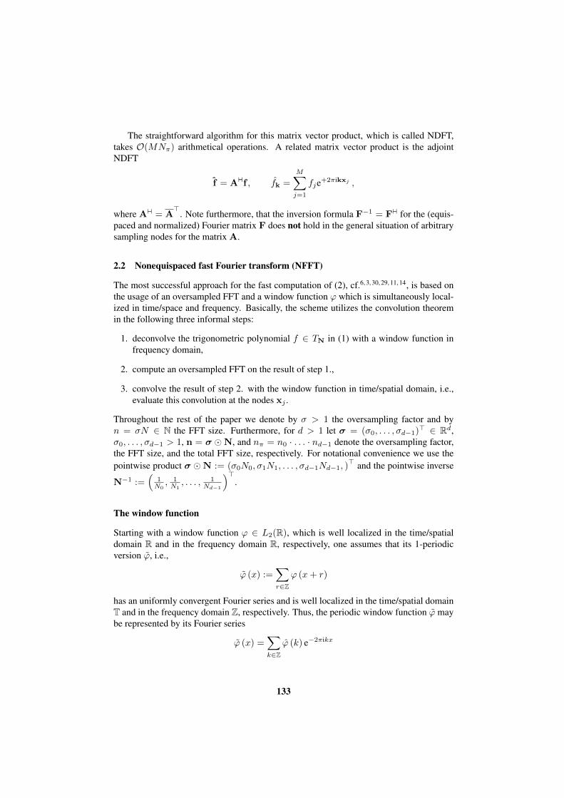
The straightforward algorithm for this matrix vector product, which is called NDFT,takes O(MNπ) arithmetical operations. A related matrix vector product is the adjointNDFT
f = Aaf , fk =
M∑j=1
fje+2πikxj ,
where Aa = A>
. Note furthermore, that the inversion formula F−1 = Fa for the (equis-paced and normalized) Fourier matrix F does not hold in the general situation of arbitrarysampling nodes for the matrix A.
2.2 Nonequispaced fast Fourier transform (NFFT)
The most successful approach for the fast computation of (2), cf.6, 3, 30, 29, 11, 14, is based onthe usage of an oversampled FFT and a window function ϕ which is simultaneously local-ized in time/space and frequency. Basically, the scheme utilizes the convolution theoremin the following three informal steps:
1. deconvolve the trigonometric polynomial f ∈ TN in (1) with a window function infrequency domain,
2. compute an oversampled FFT on the result of step 1.,
3. convolve the result of step 2. with the window function in time/spatial domain, i.e.,evaluate this convolution at the nodes xj .
Throughout the rest of the paper we denote by σ > 1 the oversampling factor and byn = σN ∈ N the FFT size. Furthermore, for d > 1 let σ = (σ0, . . . , σd−1)> ∈ Rd,σ0, . . . , σd−1 > 1, n = σ N, and nπ = n0 · . . . · nd−1 denote the oversampling factor,the FFT size, and the total FFT size, respectively. For notational convenience we use thepointwise product σ N := (σ0N0, σ1N1, . . . , σd−1Nd−1, )
> and the pointwise inverse
N−1 :=(
1N0, 1N1, . . . , 1
Nd−1
)>.
The window function
Starting with a window function ϕ ∈ L2(R), which is well localized in the time/spatialdomain R and in the frequency domain R, respectively, one assumes that its 1-periodicversion ϕ, i.e.,
ϕ (x) :=∑r∈Z
ϕ (x+ r)
has an uniformly convergent Fourier series and is well localized in the time/spatial domainT and in the frequency domain Z, respectively. Thus, the periodic window function ϕ maybe represented by its Fourier series
ϕ (x) =∑k∈Z
ϕ (k) e−2πikx
133

with the Fourier coefficients
ϕ (k) :=
∫T
ϕ (x) e+2πikx dx =
∫R
ϕ (x) e+2πikx dx , k ∈ Z.
We truncate this series at the FFT length n, which causes an aliasing error.If ϕ is furthermore well localized in time/spatial domain R, it can be truncated with
truncation parameterm ∈ N, m n and approximated by the function ϕ·χ[−mn ,mn ] which
has compact support within the interval [−mn , mn ]. Furthermore, the periodic window func-tion can be approximated by the periodic version of the truncated window function. Ford > 1, univariate window functions ϕ0, . . . , ϕd−1, and a node x = (x0, . . . , xd−1)> themultivariate window function is simply given by
ϕ (x) := ϕ0 (x0)ϕ1 (x1) . . . ϕd−1 (xd−1)
and ϕ(x) =∑
r∈Zd ϕ(x + r) again denotes the 1-periodic version; an immediate observa-tion is
ϕ (k) :=
∫Rd
ϕ (x) e+2πikx dx = ϕ0 (k0) ϕ1 (k1) . . . ϕd−1 (kd−1) .
For a single truncation parameter m ∈ N the window function is truncated to the cuben−1 [−m,m]d.
We follow the general approach of30, 29 and approximate the complex exponentials inthe trigonometric polynomial (1) by
e−2πikx ≈ 1
nπϕ (k)
∑l∈In,m(x)
ϕ(x− n−1 l
)e−2πi(n−1l)k (3)
where the set
In,m (x) := l ∈ In : n x−m1 ≤ l ≤ n x +m1collects these indices where the window function is mostly concentrated (the inequalitieshave to be fulfilled modulo n and for each component). After changing the order of sum-mation in (1) we obtain for xj ∈ Td, j = 1, . . . ,M, the approximation
f (xj) ≈∑
l∈In,m(xj)
(∑k∈IN
fknπϕ (k)
e−2πi(n−1l)k
)ϕ(xj − n−1 l
).
This causes a truncation and an aliasing error, see29, 26 for details. As can be readily seen,after an initial deconvolution step, the expression in brackets can be computed via a d-variate FFT of total size nπ . The final step consists of the evaluation of sums having atmost (2m+ 1)d terms where the window function is sampled only in the neighborhood ofthe node xj .
The algorithm and its matrix notation
The proposed scheme reads in matrix vector notation as
Af ≈ BFDf ,
134

where B denotes the real M × nπ sparse matrix
B :=(ϕ(xj − n−1 l
)· χIn,m(xj) (l)
)j=1,...,M ; l∈In
, (4)
where F is the d-variate Fourier matrix of size nπ × nπ ,
F :=(
e−2πi(n−1l)k)l∈In;k∈In
, (5)
and where D is the real nπ ×Nπ ’diagonal’ matrix
D :=
d−1⊗t=0
(Ot | diag
(1
ntϕt (kt)
)kt∈INt
|Ot
)>(6)
with zero matrices Ot of size Nt × nt−Nt2 . Obviously, the approximate matrix splitting
can be applied to the adjoint matrix as Aa ≈ D>FaB>, where the multiplication withthe sparse matrix B> is implemented in a ’transposed’ way, summation as outer loop andonly using the index sets In,m (xj).
Algorithm 2.1 NFFTInput: d ∈ N dimension,
M ∈ N number of nodes, nodes xj ∈ [− 12 ,
12 )d, j = 1, . . . ,M ,
N ∈ 2Nd multi degree, Fourier coefficients fk ∈ C, k ∈ IN,σ ∈ Rd oversampling factor with σt > 1, t = 0, . . . , d− 1,m ∈ N window size of ϕ.
1. For k ∈ IN compute
gk :=fk
nπϕ(k).
2. For l ∈ In with n = σ N compute by d-variate (forward) FFT
gl :=∑k∈IN
gk e−2πik(n−1l).
3. For j = 1, . . . ,M compute
sj :=∑
l∈In,m(xj)
gl ϕ(xj − n−1 l
).
Output: approximate values sj ≈ f(xj) , j = 1, . . . ,M .
Evaluation techniques for window functions
To keep the aliasing error and the truncation error small, several univariate functions ϕwith good localization in time and frequency domain were proposed. For an oversamplingfactor σ > 1, a degree N ∈ 2N, the FFT length n = σN , and a cut-off parameter m ∈ N,the following window functions are considered:
135

Algorithm 2.2 NFFTa
Input: d ∈ N dimension,M ∈ N number of nodes,nodes xj ∈ [− 1
2 ,12 )d, coefficients fj ∈ C, j = 1, . . . ,M ,
N ∈ 2Nd multi degree,σ ∈ Rd oversampling factor with σt > 1, t = 0, . . . , d− 1,m ∈ N window size of ϕ.
1. For l ∈ In with n = σ N compute
gl :=
M∑j=1
l∈In,m(xj)
fj ϕ(xj − n−1 l
).
2. For k ∈ In compute by d-variate (backward) FFT
gk :=∑l∈In
gl e+2πik(n−1l).
3. For k ∈ IN compute
sk :=gk
nπϕ(k).
Output: approximate values sk ≈ fk, k ∈ IN.
1. for a shape parameter b = 2σ2σ−1
mπ the dilated Gaussian window6, 30, 5
ϕ(x) = (πb)−1/2 e−(nx)2/b, (7)
ϕ(k) =1
ne−(πkn )2b,
2. for M2m denoting the centered cardinal B-Spline of order 2m the dilated B-Splinewindow3, 30
ϕ(x) = M2m(nx), (8)
ϕ(k) =1
n
1 for k = 0,
sinc2m
(kπ
n
)otherwise,
3. the dilated Sinc window26
ϕ(x) =N (2σ − 1)
2msinc2m
(πNx (2σ − 1)
2m
), (9)
ϕ(k) = M2m
(2mk
(2σ − 1)N
),
with sinc(x) := sin(x) / x for x 6= 0 and sinc(0) := 1
136

4. and for a shape parameter b = π(2− 1σ ) the dilated Kaiser-Bessel window27
ϕ(x) =1
π
sinh(b
√m2 − n2x2)√
m2 − n2x2for |x| ≤ m
n ,
sin(b√n2x2 −m2)√
n2x2 −m2otherwise,
(10)
ϕ(k) =
1n I0
(m√b2 − (2πk/n)2
)for k = −n
(1− 1
2σ
), . . . , n
(1− 1
2σ
),
0 otherwise,
where I0 denotes the modified zero-order Bessel function.
Note, that the latter two have compact support in frequency domain while the second onehas compact support in time domain. Further references on the usage of (generalized)Kaiser-Bessel window functions include18, 23, where some authors prefer to interchangethe role of time and frequency domain. For these univariate window functions ϕ, theapproximation error of Algorithm 2.1 obeys
|f (xj)− sj | ≤ Cσ,m‖f‖1 ,
where
Cσ,m :=
4 e−mπ(1−1/(2σ−1)) for (7), cf.30,
4(
12σ−1
)2m
for (8), cf.30,
1m−1
(2
σ2m +(
σ2σ−1
)2m)
for (9), cf.26,
4π (√m+m) 4
√1− 1
σ e−2πm√
1−1/σ for (10), cf.26.
Thus, for fixed σ > 1, the approximation error introduced by the NFFT decays exponen-tially with the number m of terms in sum (3). Using the tensor product approach, the errorestimates above have been generalized for the multivariate setting in7, 5.
In summary, the whole algorithm for the fast approximate computation of (1) consistsof the computation of Nπ multiplications, the computation of a d-variate FFT of total sizenπ and the sparse summations. Therefore it requiresO(nπ +nπ log nπ +(2m+1)dM) =O(nπ log nπ +mdM) arithmetic operations.
In21 we suggest different methods for the compressed storage and application of ma-trix B, which are all available within our NFFT library19 by choosing particular flags ina simple way during the initialization phase. These methods include fully precomputedwindow function, tensor product based precomputation, linear interpolation from a lookuptable, fast Gaussian gridding (see also14) and no precomputation of the window function.The choice of precomputation does not yield a different asymptotic performance but ratheryields a lower constant in the amount of computation.
Finally we remark, that similar approximations of the exponentials as in (3) are used invarious particle methods, see [4, Formula (24)], [8, Formula (3.5)] or [15, Formula (7.57)].However, mainly splines are used as window functions. We note that, e.g., Kaiser-Besselfunctions lead to better results, while using the same window size m, see Figure 1 and20,
137

0 5 10 1510
−15
10−10
10−5
100
(a) d = 1, N = 212.0 5 10 15
10−15
10−10
10−5
100
(b) d = 2, N = 26.0 5 10 15
10−15
10−10
10−5
100
(c) d = 3, N = 24.
Figure 1: Error E∞ for increasing cut-off parameter m = 0, . . . , 14 and d = 1, 2, 3. In each case, the degreeN was chosen to be equal along each dimension such that |IN| = 212. We fixed the oversampling factor σ = 2and M = 10000. Shown are results for the Kaiser-Bessel (), the Sinc (×), the B-spline (+), and the Gaussianwindow function (4).
where the accuracy is measured by
E∞ := max1≤j≤M
|fj − sj |/∑k∈IN
|fk| .
For further NFFT approaches see [20, Appendix D].
3 Fast Summation Algorithms
We are interested in the fast evaluation of sums
h(y) :=
L∑l=1
αlK(y − xl) =
L∑l=1
αlK(‖y − xl‖2), (11)
at M different target nodes yj , j = 1, . . . ,M , where ‖x‖2 := (x20 + . . . + x2
d−1)1/2
denotes the Euclidean norm. This approach was suggested in27, 28, 9. The original idea forour algorithm came from the consideration of (11) for equispaced source nodes xl andtarget nodes yj . In this case we have simply to compute the multiplication of a vector witha Toeplitz matrix or a block–Toeplitz–Toeplitz–block matrix in the multivariate setting.The standard algorithm to do this uses the FFT, see [27, Section2]. Here we propose thesummation algorithm based on NFFT for arbitrary distributed source and target nodes.
The kernel function K is in general a non-periodic function, while the use of Fouriermethods requires to replace K by a periodic version. Without loss of generality we mayassume that the source and target nodes are scaled, such that ‖xl‖2, ‖yj‖2 < 1
4 − εB2 and
consequently ‖yj − xl‖2 < 12 − εB. The parameter εB > 0, which we specify later,
guarantees that K has to be evaluated only at nodes in the ball with radius 12 − εB. This
simplifies the later consideration of a 1-periodic version of K.We deal with kernels K which are C∞ except for the origin, where K or its derivatives
may have singularities. Examples of such kernels are
‖x‖22 log ‖x‖2, log ‖x‖2 and1
‖x‖β2(β ∈ N).
138

For the sake of simplicity we define K(0) = 0 whenever a singularity appears at theorigin. This enables us to evaluate (11) at source nodes which coincide with a targetnode. Of course, our algorithm can be modified for other kernels frequently used in the ap-proximation by radial basis functions, e.g., the Gaussian22 or the (inverse) multiquadric10
(x2 + c2)±1/2. Our algorithm, in particular our regularization procedure, is simply struc-tured, can easily be adapted to different kernels K and requires O(L log d
√L + M) or
O(M log d√M + L) arithmetic operations for uniformly distributed source nodes xl or
target nodes yj , respectively.Beyond a special treatment of K near the boundary, we have to be concerned about the
singularity of K at the origin. We regularize K near 0 and near the boundary x ∈ Td :‖x‖2 = 1
2 as follows
KR(x) :=
TI(‖x‖2) if ‖x‖2 ≤ εI,
TB(‖x‖2) if 12 − εB < ‖x‖2 < 1
2 ,
TB( 12 ) if 1
2 ≤ ‖x‖2,K(‖x‖2) otherwise,
(12)
where 0 < εI <12 − εB < 1
2 . The functions TI and TB will be chosen such that KR is inthe Sobolev space Hp(Td) for an appropriate parameter p ∈ N. Several regularizations ofK are possible, e.g., by algebraic polynomials, splines or trigonometric polynomials, see10.
Here we focus our attention on two point Taylor interpolation, i.e., we are interested inthe unique polynomial of degree 2p− 1 which satisfies the interpolation conditions
P (j)(m− r) = aj , P (j)(m+ r) = bj , j = 0, . . . , p− 1 (13)
at the endpoints of an interval [m− r,m+ r], r > 0.Lemma 3.1. (see [9, Proposition 2.2]) For given aj , bj (j = 0, . . . , p − 1) there exists aunique polynomial P of degree 2p−1 which satisfies (13). With y := z−m
r this polynomialcan be written as
P (z) =1
2p
p−1∑j=0
p−1−j∑k=0
(p− 1 + k
k
)rj
j!2k((1 + y)j+k(1− y)paj + (1− y)j+k(1 + y)p(−1)jbj
).
(14)
Lemma 3.2. The derivative of the polynomial P from (14) is given by
P ′(z) =1
2p
p−1∑j=0
p−1−j∑k=0j+k 6=0
(p− 1 + k
k
)rj−1
j!2k
((1 + y)j+k−1(1− y)p−1
[(j + k)(1− y)− p(1 + y)
]aj
+ (1− y)j+k−1(1 + y)p−1[(j + k)(1 + y)− p(1− y)
](−1)j−1bj
).
(15)
We exploit (14) with aj = K(j)(εI), bj = (−1)jaj , j = 0, . . . , p− 1,m = 0, r = 2εI
to obtain TI and with aj = K(j)( 12−εB), bj = δ0,jK( 1
2 ), j = 0, . . . , p−1,m = 1−εB2 , r =
εB to obtain TB.
139

Next we approximate the smooth function KR by the Fourier series
KR ≈ KRF(x) :=∑k∈IN
bke−2πikx, (16)
where
bk :=1
Nπ
∑l∈IN
KR(N−1 l)e+2πi(N−1l)k, k ∈ IN . (17)
Then our original kernel splits as
K = (K −KR) + (KR −KRF) + KRF = KNE + KER + KRF, (18)
where KNE := K −KR and KER := KR −KRF. Since KR is smooth, the approximationerror KER of its Fourier approximation KRF should be small. We neglect this error andapproximate h in (11) by
h(y) ≈ h(y) := hNE(y) + hRF(y),
where
hNE(y) :=
L∑l=1
αlKNE(y − xl) , (19)
hRF(y) :=
L∑l=1
αlKRF(y − xl) . (20)
Instead of h we evaluate h at the target nodes yj . If either the source nodes xk or the targetnodes yj are “sufficiently uniformly distributed” this can indeed be done in a fast way,namely:
Near field computation (19)
By definition (12), the function KNE has a small support contained in the ball of radiusεI around 0 and in the neighborhood of the boundary. The boundary is not interesting forus since ‖yj − xl‖2 ≤ 1/2 − εB. To achieve the desired complexity of our algorithmwe suppose that either the L source nodes xl or the M target nodes yj are “sufficientlyuniformly distributed”, i.e., we suppose that there exists a small constant ν ∈ N such thatevery ball of radius εI contains at most ν of the nodes xl or of the nodes yj , respectively.This implies that εI depends linearly on 1/ d
√L, respectively 1/ d
√M . In the following, we
restrict our attention to the case
εI ∼ d
√ν
L.
Then for fixed yj the sum (19) contains not more than ν terms so that its evaluation at Mtarget nodes yj requires only O(νM) arithmetic operations.
We remark that also O(log d√M), respectively O(log d
√L) nodes instead of O(1)
nodes per ball will keep a complexity of O(M log d√M + L log d
√L) of our whole al-
gorithm.
140

Far field summation (20) by NFFTa/NFFT
Substituting (16) for KRF we obtain
hRF(yj) =
L∑l=1
αl∑k∈IN
bke−2πik(yj−xl) =∑k∈IN
bk
(L∑l=1
αle+2πikxl
)e−2πikyj .
The expression in the inner brackets can be computed by a d-variate NFFTa of total sizeNπ . This is followed by Nπ multiplications with bk and completed by a d-variate NFFT oftotal size Nπ to compute the outer sum with the complex exponentials. If m is the cut-offparameter and σ = (2)t=0,...,d−1 the oversampling factor of the NFFTa/NFFT, then theproposed evaluation of hRF at the nodes yj , j = 1, . . . ,M requires O(md(L + M) +σπNπ log(σπNπ)) arithmetic operations. The relation between M,L and N is determinedby the approximation error of the algorithm and is discussed in detail in27, 28, 10.
Note, we can avoid the error ofKER in the near field in (18) by splitting kernel functionK as
K = (K −KRF) + KRF = KNE + KER + KRF, (21)
and setting KNE := (K −KRF)χ‖·‖≤εI, KER := K − KRF − KNE. The first splitting(18) is preferable, if we are able to evaluate the near field regularization TI in a fast way. IfTI can not be computed in a fast way but the Fourier coefficients bk are given, the splitting(21) should be used.
The algorithm and its matrix notation
The proposed scheme reads in matrix vector notation as
Kα ≈ ByFDDbD>FHB>x α+ KNEα , (22)
where Bx denotes the real L × nπ sparse matrix depending on the source nodes xl, l =1, . . . , L as given in (4)
Bx :=(ϕ(xl − n−1 l
)· χIn,m(xl) (l)
)l=1,...,L; l∈In
,
By denotes the realM×nπ sparse matrix depending on the target nodes yj , j = 1, . . . ,Mas given in (4)
By :=(ϕ(yj − n−1 l
)· χIn,m(yj) (l)
)j=1,...,M ; l∈In
,
F is the d-variate Fourier matrix of size nπ ×nπ given in (5), D is the real nπ ×Nπ ’diag-onal’ matrix given in (6), which contains the Fourier coefficients of the window function,Db = diag(bk)k∈IN contains the Fourier coefficients of the regularized kernel KR givenin (17). Furthermore, KNE contains the near field correction (19). From the representation(22) we see, that FDFH with a diagonal matrix D is well known as fast realization of aconvolution on a mesh. The matrix B> is used to smear the charge density onto a grid,then one can use a convolution on a mesh and finally a back-interpolation via B.
In summary we obtain Algorithm 3.1 for the fast evaluation of (11).
141

Algorithm 3.1 Fast sumInput: d ∈ N dimension,
p ∈ N smoothness of regularized kernel KR,N ∈ 2Nd multi degree,εI > 0 nearfield size,εB > 0 boundary size,L ∈ N number of source nodes,M ∈ N number of target nodes,source nodes xl ∈ [− 1
4 + εB2 ,
14 − εB
2 )d, l = 1, . . . , L,target nodes yj ∈ [− 1
4 + εB2 ,
14 − εB
2 )d, j = 1, . . . ,M ,coefficients αl ∈ C, l = 1, . . . , L.
Precomputation:
i) Computation of (bk)k∈IN by (17) and (12).
ii) Computation of KNE(yj − xl) for all j = 1, . . . ,M and l ∈ INEεI (j),
where INEεI (j) := l ∈ 1, . . . , L : ‖yj − xl‖2 < εI.
1. For k ∈ IN compute by Algorithm 2.2 the d-variate NFFTa
ak :=
L∑l=1
αle+2πikxl .
2. For k ∈ IN compute the products
dk := akbk.
3. For j = 1, . . . ,M compute by Algorithm 2.1 the d-variate NFFT
hRF(yj) :=∑k∈IN
dke−2πikyj .
4. For j = 1, . . . ,M compute the near field sums
hNE(yj) =∑
l∈INEεI
(j)
αlKNE(yj − xl).
5. For j = 1, . . . ,M compute the near field corrections
h(yj) = hNE(yj) + hRF(yj).
Output: approximate values h(yj) ≈ h(yj), j = 1, . . . ,M .
Generalization to cuboidal domains
Whenever the restrictions ‖xl‖2, ‖yj‖2 < 14 − εB
2 are not fulfilled we must scale thenodes. We now explain the resulting changes to Algorithm 3.1. In order to handle nodedistributions with unequal dimensional extend we introduce s = (s0, s1, . . . , sd−1)> ∈ Nd
142

as a component wise scaling such that ‖s−1 xl‖2, ‖s−1 yj‖2 < 14 −
εB
2 and therefore‖s−1 (yj − xl)‖ < 1
2 − εB for all l = 1, . . . , L and j = 1, . . . ,M . By the substitutionz := s−1 x we obtain x = s z and therefore Ks(z) := K(s z) = K(x).
Since Ks is not radial symmetric anymore, we define the regularized kernel functionKs
R in a slightly different way
KsR(z) :=
TI(‖s z‖2) if ‖s z‖2 ≤ εI,
T zB(‖z‖2) if 1
2 − εB < ‖z‖ < 12 ,
T zB( 1
2 ) if 12 ≤ ‖z‖,
K(‖s z‖2) otherwise.
While the definition of TI remains the same as in the non-scaled case, we again ex-ploit (14) to obtain T z
B with the altered parameters aj = K(j)(( 12 − εB)‖sz‖2‖z‖2 ), bj =
δ0,jK( 12smax), j = 0, . . . , p − 1,m = 1
2 − εB2 , r = εB, where smax := maxst : t =
0, . . . , d−1. Note that the interpolation polynomial T zB may change for every node, since
the coefficients aj now depend on z. We only need to evaluate T zB during a precompu-
tation step to obtain the Fourier coefficients bk of the regularized kernel function KRF,therefore the dependency of the interpolation polynomial on z has no impact on the com-plexity of our fastsum algorithm. In order to assure differentiability of KRF at the borderx ∈ Td : ‖x‖2 ≥ 1
2, we set T zB( 1
2 ) = b0 constant for all z.Let sπ := s0 · . . . ·sd−1. We approximate the smooth functionKs
R by the Fourier series
KsRF(x) :=
∑k∈IsN
bke−2πikx,
where the Fourier coefficients bk are given by the d-variate discrete Fourier transform
bk =1
sπNπ
∑l∈IsN
KsR(s−1 N−1 l)e+2πi(s−1N−1l)k, k ∈ IsN.
The remaining part of the fast summation algorithm can be done analogously to the non-scaled case with the scaled NFFT size sN instead of N.
4 Application to Particle Simulation for the Coulomb Potential
In this part we apply our fast summation algorithm to the long-range potential 1/r. Thefundamental idea is to split the long-range part of the potential into a smooth long-rangepart and a singular short range part. We will use our splitting (19) and (20). There ex-ists a variety of methods which use similar splittings such as the P 3M method17. In thefollowing we will discuss open and periodic systems.
4.1 Open systems
In this part we apply our fast summation algorithm to a system of M charged particleslocated at source nodes xl ∈ R3 with charge ql ∈ R. We are interested in the evaluation ofthe electrostatic potential φ at target node y ∈ R3,
φ(y) :=
M∑l=1
qlK(y − xl), (23)
143

and the force F acting at particle y ∈ R3 with charge q(y) ∈ R,
F(y) := −q(y)∇φ(y) = −q(y)
M∑l=1
qlK′(y − xl), (24)
where the kernel functions K and K′ corresponding to the Coulomb potential are given by
K(x) =
0 if ‖x‖2 = 0,1/‖x‖2 otherwise, and K′(x) =
0 if ‖x‖2 = 0,x/‖x‖32 otherwise. (25)
For equal sets of source and target nodes the sum (23) turns into
φ(xj) =
M∑l=1l 6=j
ql‖xj − xl‖2
, j = 1, . . . ,M,
and (24) becomes
F(xj) = −qjM∑l=1l 6=j
qlxj − xl‖xj − xl‖32
, j = 1, . . . ,M.
Furthermore we are interested in the computation of the total electrostatic potential energy
U :=1
2
M∑j=1
qjφ(xj),
which can be evaluated straightforward after the computation of the potentials φ(xj), j =1, . . . ,M . To get the potentials φ(xj) we apply Algorithm 3.1 on (23) by choosing equalsets of source and target nodes and αl = ql, l = 1, . . . ,M . For the near field correctionsof this algorithm we require repeated evaluations of the near field interpolation polynomialTI. Instead of using (14) it is more efficient to calculate the coefficients once explicitly forsmoothness p = 2, . . . , 12 and evaluate the polynomial with a Horner scheme. E.g., forsmoothness p = 5 we get the following explicit representation
TI(‖x‖2) =315
128εI+
(−105
32ε3I
+
(189
64ε5I
+
(−45
32ε7I
+35
128ε9I
‖x‖22)‖x‖22
)‖x‖22
)‖x‖22.
For the fast calculation of the forces F(y) we follow the main steps of Algorithm 3.1. Firstwe observe that Algorithm 3.1 decomposes potential φ(y) into
φ(y) ≈ φNE(y) + φRF(y), (26)
where the near field part φNE is given by
φNE(y) =
M∑l=1
‖y−xl‖2<εI
ql (K(y − xl)− TI(‖y − xl‖2))
and the far field part φRF reads as
φRF(y) =∑k∈IN
bk
(M∑l=1
qle+2πikxl
)e−2πiky.
144

Combination of (24) and (26) yields
F(y) = −q(y)∇φ(y) ≈ −q(y)(∇φNE(y) +∇φRF(y)).
Taking into account that
∇φRF(y) = −2πi∑k∈IN
bkk
(M∑l=1
qle+2πikxl
)e−2πiky,
we are able to compute the inner sum of the far field part∇φRF with only one NFFTa andthe outer vector sum with three NFFTs, one for each component. This is a remarkable im-provement to the algorithm proposed in25 where four NFFTas and four NFFTs are neededto calculate the far field part of the forces. The gradient of the near field part reads as
∇φNE(y) =
M∑l=1
‖y−xl‖2<εI
ql (K′(y − xl)−∇TI(‖y − xl‖2)) .
This vector sum can be evaluated straightforward. One way to obtain the gradient of TI isto use (15) and the chain rule with z = ‖x‖2. We obtain for ‖x‖ 6= 0
∇TI(‖x‖2) =1
2px
‖x‖2
p−1∑j=0
p−1−j∑k=0j+k 6=0
(p− 1 + k
k
)rj−1
j!2k
((1 + y)j+k−1(1− y)p−1
[(j + k)(1− y)− p(1 + y)
]aj
+ (1− y)j+k−1(1 + y)p−1[(j + k)(1 + y)− p(1− y)
](−1)j−1bj
),
where y = ‖x‖2−mr and ∇TI(0) = 0. Alternatively we represent the gradient of TI, e.g.,
for smoothness p = 5, by
∇TI(‖x‖2) =
(−105
16ε3I
+
(189
16ε5I
+
(−1080
128ε7I
+35
16ε9I
‖x‖22)‖x‖22
)‖x‖22
)x.
In summary we can apply Algorithm 3.1 with the matrix representation given in (22).
4.2 Periodic systems
In this section we present a straightforward method, that accelerates the traditional Ewaldsummation technique by NFFT. This combination was first presented in16 and is very simi-lar to the FFT-accelerated Ewald sum, namely, the so-called particle-particle particle-mesh(P3M), particle-mesh Ewald (PME) and smooth particle-mesh Ewald (SPME), see4. Ad-ditionally we will see, that the accelerated Ewald summation can be reinterpreted into amethod very similar to our fastsum Algorithm 3.1.
We consider a system of charged particles coupled via the Coulomb potential, a cubicsimulation box with edge length B, containing M charged particles, each with a chargeql ∈ R, located at xl ∈ BT3. Periodic boundary conditions in a system without cut-off is
145
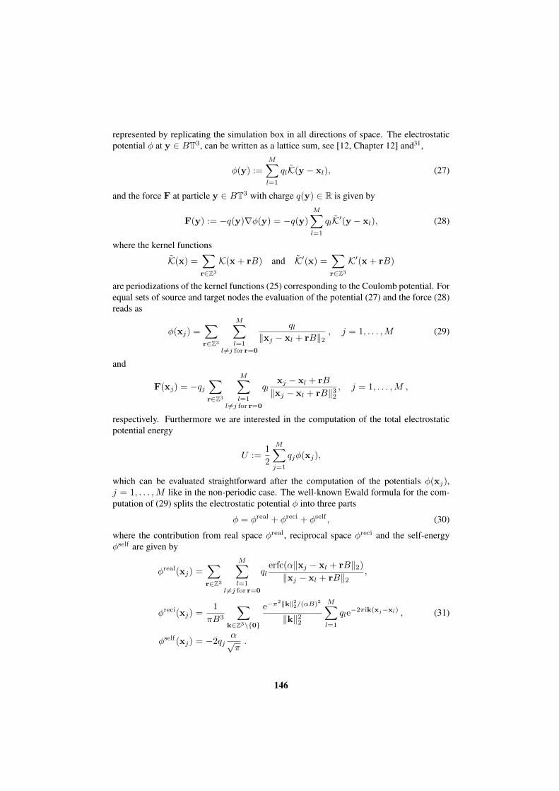
represented by replicating the simulation box in all directions of space. The electrostaticpotential φ at y ∈ BT3, can be written as a lattice sum, see [12, Chapter 12] and31,
φ(y) :=
M∑l=1
qlK(y − xl), (27)
and the force F at particle y ∈ BT3 with charge q(y) ∈ R is given by
F(y) := −q(y)∇φ(y) = −q(y)
M∑l=1
qlK′(y − xl), (28)
where the kernel functions
K(x) =∑r∈Z3
K(x + rB) and K′(x) =∑r∈Z3
K′(x + rB)
are periodizations of the kernel functions (25) corresponding to the Coulomb potential. Forequal sets of source and target nodes the evaluation of the potential (27) and the force (28)reads as
φ(xj) =∑r∈Z3
M∑l=1
l 6=j for r=0
ql‖xj − xl + rB‖2
, j = 1, . . . ,M (29)
and
F(xj) = −qj∑r∈Z3
M∑l=1
l 6=j for r=0
qlxj − xl + rB
‖xj − xl + rB‖32, j = 1, . . . ,M ,
respectively. Furthermore we are interested in the computation of the total electrostaticpotential energy
U :=1
2
M∑j=1
qjφ(xj),
which can be evaluated straightforward after the computation of the potentials φ(xj),j = 1, . . . ,M like in the non-periodic case. The well-known Ewald formula for the com-putation of (29) splits the electrostatic potential φ into three parts
φ = φreal + φreci + φself , (30)
where the contribution from real space φreal, reciprocal space φreci and the self-energyφself are given by
φreal(xj) =∑r∈Z3
M∑l=1
l 6=j for r=0
qlerfc(α‖xj − xl + rB‖2)
‖xj − xl + rB‖2,
φreci(xj) =1
πB3
∑k∈Z3\0
e−π2‖k‖22/(αB)2
‖k‖22
M∑l=1
qle−2πik(xj−xl) , (31)
φself(xj) = −2qjα√π.
146

Thereby, the complementary error function is defined by erfc(z) = 2√π
∫∞z
e−t2
dt. Choos-
ing optimal parameters, Ewald summation scales as O(M3/2). In order to overcome thisincrease in time we apply the NFFT for the calculation of the reciprocal-space potentialφreci and we obtain a method similar as our fast summation method. To this end, wecompute the Fourier transformed charge density
S(k) =
M∑l=1
qle+2πikxl
by NFFTa and after truncation of the sum (31) we obtain by NFFT
φreci(xj) ≈1
πB3
∑k∈IN\0
e−π2‖k‖22/(αB)2
‖k‖22S(k)e−2πikxj .
We now reinterpret the approximation steps of Ewald summation in order to use thesteps of our Algorithm 3.1. Following (12) we define the slightly different regularizationKR of the kernel function K by
KR(x) := TI(‖x‖2) ≈TI(‖x‖2) if ‖x‖2 ≤ εI,
K(‖x‖2) otherwise,
where the near field regularization TI is given by
TI(z) =
2α/√π if z = 0,
erf(αz)/z otherwise.
Here the error function is defined by erf(z) = 2√π
∫ z0
e−t2
dt and the parameter α mustbe chosen large enough to ensure TI(x) ≈ K(x) for all ‖x‖2 ≥ εI. Since the periodicregularization KR(x) :=
∑r∈Z3 KR(x + r) is smooth at the domain border, we do not
need a regularization TB. Instead of (30) we use (18) to split the electrostatic potential φfrom (27) into the two parts
φ(y) ≈ φNE(y) + φRF(y),
where the near field part φNE is given by
φNE(y) =
M∑l=1
‖y−xl‖2<εI
ql
(K(y − xl)− TI(‖y − xl‖2)
)
and the far field part φRF reads as
φRF(y) =∑k∈IN
bk
(M∑l=1
qle+2πikxl
)e−2πiky.
Since the Fourier coefficients bk of KR can be calculated analytically,
bk =
0 if ‖k‖2 = 0,e−π
2‖k‖22/(αB)2
‖k‖22otherwise,
147

we do not need to compute an inverse discrete Fourier transformation of KR in the pre-computation step as in (17). Analogously to Algorithm 3.1 the far field part φRF can beevaluated by one NFFTa and one NFFT, while the near field part only includes nearestneighbors of every target node. Therefore we get an algorithm with the same complexityas our fastsum algorithm for non-periodic systems. For equal sets of source and targetnodes the resulting algorithm coincides with the NFFT-accelerated Ewald summation.
As in the non-periodic case we get
F(y) = −q(y)∇φ(y) ≈ −q(y)(∇φNE(y) +∇φRF(y)),
where the far field part ∇φRF(y) can be computed by one NFFTa and three NFFTs. Thenear field part ∇φNE(y) reads as
∇φNE(y) =
M∑l=1
‖y−xl‖2<εI
ql (K′(y − xl)−∇TI(‖y − xl‖2)) .
This vector sum can be evaluated straightforward. Since
d
dz
erf(αz)
z=
1
z
(2α√π
e−α2z2 − erf(αz)
z
)the gradient of TI is given by
∇TI(‖x‖2) =
0 if ‖x‖2 = 0,
x‖x‖22
(2α√π
e−α2‖x‖22 − erf(α‖x‖2)
‖x‖2
)otherwise.
For equal sets of source and target nodes we get
F(xj) ≈ FNE(xj) + FRF(xj),
whereFNE(xj) =− qj∇φNE(xj)
=− qjM∑l=1l 6=j
qlxj − xl‖xj − xl‖22
(erfc(α‖xj − xl‖2)
‖xj − xl‖2+
2α√π
e−α2‖xj−xl‖22
),
FRF(xj) =− qj∇φRF(xj)
=2iqjB3
∑k∈IN\0
e−π2‖k‖22/(αB)2
‖k‖22kS(k)e−2πikxj .
This splitting coincides with the well known results of Ewald summation.In summary we can apply Algorithm 3.1 with the matrix representation given in (22).
5 Numerical Results
5.1 Generation of pseudo random sampling sets
To guarantee a minimum distance between all nodes we used Hammersley and Haltonpseudo random node distributions33. Let p ∈ N prime. Every non-negative integer j ∈
148

N ∪ 0 can be uniquely represented as
j = a0 + a1p+ a2p2 + . . .+ arp
r, ai ∈ 0, . . . , p− 1 , i = 0, . . . , r, r ∈ N.
We define
Φp(j) :=a0
p+a1
p2+a2
p3+ . . .+
arpr+1
.
For d given primes p1 < p2 < . . . < pd the d-variate Hammersley distribution is given bythe following M nodes(
j
M,Φp1(j),Φp2(j), . . . ,Φpd−1
(j)
)>, j = 0, . . . ,M − 1
and the d-variate Halton distribution consists of the M nodes
(Φp1(j),Φp2(j), . . . ,Φpd(j))>, j = 0, . . . ,M − 1.
Note that it is possible to increase a given set of Halton distributed nodes, while the numberof Hammersley distributed nodes must be fixed because of the dependency of the firstcomponent of every node on M . Both distributions were implemented in2. The softwarepackage called HAMMERSLEY contains algorithms to generate Hammersley and Haltondistributions on the square [0, 1]
2 and the cube [0, 1]3. Furthermore it includes routines
for mapping the square [0, 1]2 to the sphere x ∈ R3 : ‖x‖2 = 1 and mapping the cube
[0, 1]3 to the ball x ∈ R3 : ‖x‖2 ≤ 1.
5.2 Error definitions
We performed the computations of the total energy U , the potentials φ(xj) and the forcesF(xj) for different node distributions with the direct algorithm, the fast multipole methodfrom FCS software library1 and the NFFT based algorithms. In this section we use thenames of the applied methods to label numerical results, e.g., Udirect, UFMM and UNFFT
holds the results of the energy computations based on the three algorithms, respectively.We used the following error measurements to compare the results produced by the threemethods.
The relative errors of the total potential energy with respect to the applied method readas
EFMMU :=
UFMM
Udirect, ENFFT
U :=UNFFT
Udirect.
Let φ = (φ(x1), . . . , φ(xM ))>. The relative errors of the potential with respect to theapplied method are given by
EFMMφ :=
‖φdirect − φFMM‖2‖φdirect‖2
, ENFFTφ :=
‖φdirect − φNFFT‖2‖φdirect‖2
.
For F(x) = (F0(x), F1(x), F2(x))>, and Ft := (Ft(x0), . . . , Ft(xM ))>, t = 0, 1, 2, wedefine the average relative errors of the forces with respect to the applied method via
EFMMF :=
1
3
2∑t=0
‖Fdirectt − FFMM
t ‖1‖Fdirect
t ‖1, ENFFT
F :=1
3
2∑t=0
‖Fdirectt − FNFFT
t ‖1‖Fdirect
t ‖1.
149

5.3 Test casesWe computed all test cases on the nowadays retired JUMP cluster at Research CenterJulich. Each of its 41 nodes got 32 Power4+ processors at 1.7 GHz and 128 GB memory.Our test runs were performed on one processor of one completely allocated node. The FCSsoftware library1 (timestamp 16.08.2007) and the NFFT library were compiled with IBM’sxlf and xlc compilers at optimization level -O5 and with the flag -q64 to support the 64 bitarchitecture of JUMP.
We performed the NFFT based fastsum algorithm with equal oversampling factorsσt = 2, t = 0, 1, 2, the truncation parameter m = 2, choose the Kaiser-Bessel windowfunction, the regularization parameter p = 5 and set the initialization flags PRE PHI HUT,PRE LIN PSI, FFT OUT OF PLACE, FFTW MEASURE and FFTW DESTROY INPUTto obtain the following results.
The upper bound of the relative error of the total energy UFMM was set to 0.001 forthe FMM based calculations. For the NFFT based computations we tried to adjust theparameters to obtain the same upper bound on UNFFT. All measured times include thecomputation of the energy, the potentials and the forces.
Hammersley distribution within a cubeFor this test caseM nodes satisfy a Hammersley distribution with parameters p1 = 2, p2 =3 on [0, 1]
3. The randomly chosen charges ql ∈ −1, 1 fulfillM∑l=1
ql ∈ −1, 0, 1 .
0
0.2
0.4
0.6
0.8
1 0 0.2
0.4 0.6
0.8 1
0
0.2
0.4
0.6
0.8
1
Figure 2: Hammersley distribution within a cube for 500 nodes.
Hammersley distribution within a ballFor this test case a Hammersley distribution with parameters p1 = 2, p2 = 3 on [0, 1]
3 ismapped to the ball
(x− 0.5)2 + (y − 0.5)2 + (z − 0.5)2 ≤ (0.5)2.
150

M N εI = εB tdirect tFMM tNFFT
500 (32,32,32)> 3/32 0.01 0.01 0.115 000 (32,32,32)> 3/32 0.86 0.25 0.38
50 000 (64,64,64)> 3/64 87.09* 3.00 4.63
Table 1: Runtimes t in seconds of direct, FMM and NFFT based computations, respectively. The nodes satisfy aHammersley distribution in a cube. Times with ∗ are estimated.
M EFMMU ENFFT
U EFMMφ ENFFT
φ EFMMF ENFFT
F
500 1.544e-15 3.094e-04 1.603e-15 8.086e-04 1.689e-15 1.917e-035 000 1.668e-07 9.205e-05 2.571e-06 5.626e-04 7.270e-06 9.513e-04
50 000 2.388e-08 3.006e-04 3.222e-07 5.454e-04 8.060e-07 1.240e-03
Table 2: Errors EU of total potential energy, Eφ of the potential and EF of the forces for FMM and NFFT,respectively. The nodes satisfy a Hammersley distribution in a cube.
The randomly chosen charges ql ∈ −1, 1 fulfill
M∑l=1
ql ∈ −1, 0, 1 .
0
0.2
0.4
0.6
0.8
1 0
0.2
0.4
0.6
0.8
1
0
0.2
0.4
0.6
0.8
1
Figure 3: Hammersley distribution within a ball for 500 nodes.
Cylindrical Halton distribution
For this test case a Halton distribution with parameters p1 = 2, p2 = 3, p3 = 5 on thecylinder
0 ≤ x0 ≤ 10, (x1 − 0.5)2 + (x2 − 0.5)2 ≤ 1
151

M N εI = εB tdirect tFMM tNFFT
500 (32,32,32)> 3.5/32 0.01 0.01 0.115 000 (32,32,32)> 3.5/32 0.86 0.24 0.34
50 000 (64,64,64)> 3.5/64 87.06 3.47 4.20500 000 (128,128,128)> 3.5/128 8903.23 46.77 59.48
Table 3: Runtimes t in seconds of direct, FMM and NFFT based computations, respectively. The nodes satisfy aHammersley distribution in a ball.
M EFMMU ENFFT
U EFMMφ ENFFT
φ EFMMF ENFFT
F
500 9.677e-16 5.584e-05 1.751e-15 4.189e-04 2.328e-15 1.092e-035 000 1.339e-06 4.903e-05 5.471e-06 3.190e-04 1.454e-05 6.404e-04
50 000 1.113e-07 4.087e-04 2.579e-07 2.507e-04 7.650e-07 7.416e-04500 000 1.075e-09 3.726e-04 7.366e-08 2.962e-04 2.195e-07 7.613e-04
Table 4: Errors EU of total potential energy, Eφ of the potential and EF of the forces for FMM and NFFT,respectively. The nodes satisfy a Hammersley distribution in a ball.
is scaled into the cube [0, 1]3. The randomly chosen charges ql ∈ −1, 1 fulfill
M∑l=1
ql ∈ −1, 0, 1 .
0
0.2
0.4
0.6
0.8
1 0
0.2
0.4
0.6
0.8
1
0
0.2
0.4
0.6
0.8
1
Figure 4: Cylindrical Halton distribution for 500 nodes.
152
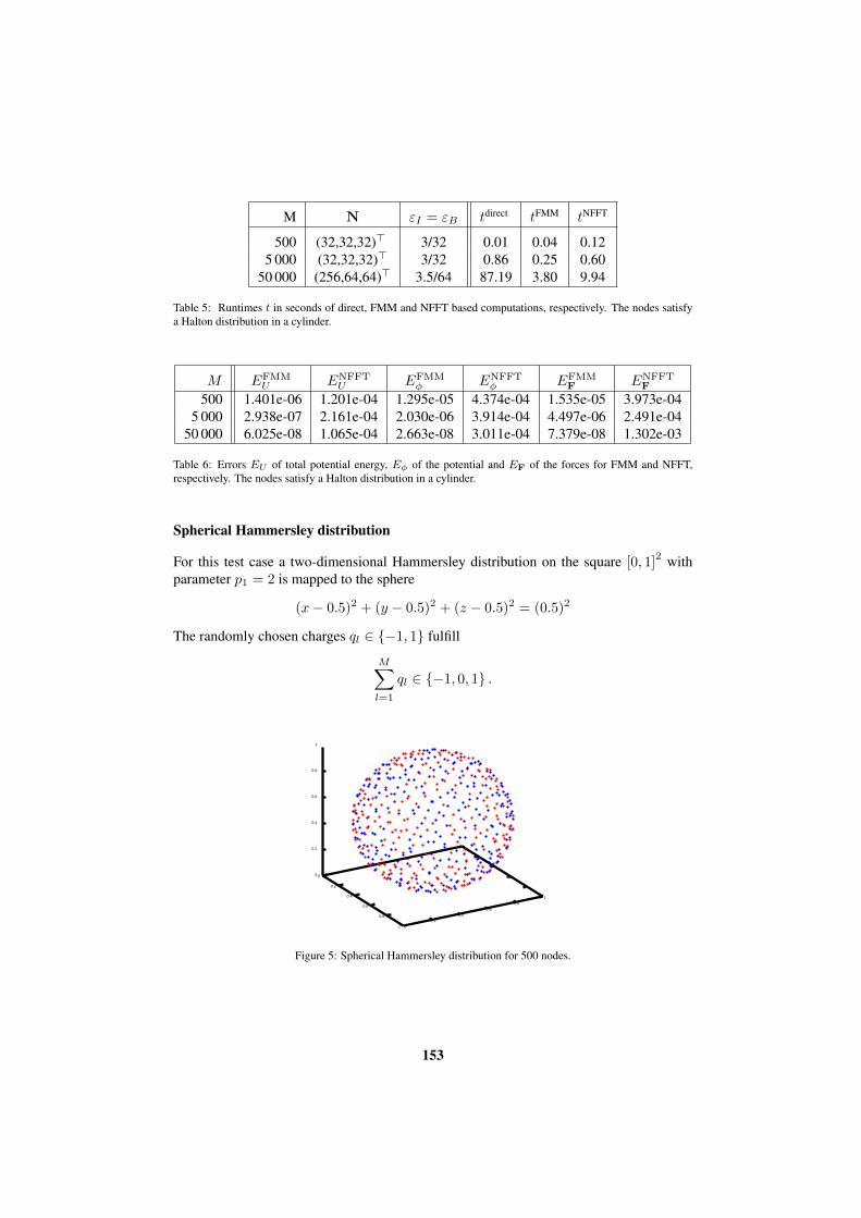
M N εI = εB tdirect tFMM tNFFT
500 (32,32,32)> 3/32 0.01 0.04 0.125 000 (32,32,32)> 3/32 0.86 0.25 0.60
50 000 (256,64,64)> 3.5/64 87.19 3.80 9.94
Table 5: Runtimes t in seconds of direct, FMM and NFFT based computations, respectively. The nodes satisfya Halton distribution in a cylinder.
M EFMMU ENFFT
U EFMMφ ENFFT
φ EFMMF ENFFT
F
500 1.401e-06 1.201e-04 1.295e-05 4.374e-04 1.535e-05 3.973e-045 000 2.938e-07 2.161e-04 2.030e-06 3.914e-04 4.497e-06 2.491e-04
50 000 6.025e-08 1.065e-04 2.663e-08 3.011e-04 7.379e-08 1.302e-03
Table 6: Errors EU of total potential energy, Eφ of the potential and EF of the forces for FMM and NFFT,respectively. The nodes satisfy a Halton distribution in a cylinder.
Spherical Hammersley distribution
For this test case a two-dimensional Hammersley distribution on the square [0, 1]2 with
parameter p1 = 2 is mapped to the sphere
(x− 0.5)2 + (y − 0.5)2 + (z − 0.5)2 = (0.5)2
The randomly chosen charges ql ∈ −1, 1 fulfill
M∑l=1
ql ∈ −1, 0, 1 .
0
0.2
0.4
0.6
0.8
1 0
0.2
0.4
0.6
0.8
1
0
0.2
0.4
0.6
0.8
1
Figure 5: Spherical Hammersley distribution for 500 nodes.
153

M N εI = εB tdirect tFMM tNFFT
500 (32,32,32)> 3/32 0.01 0.01 0.115 000 (32,32,32)> 3/32 0.86 0.17 0.23
50 000 (64,64,64)> 3/64 87.13 2.58 3.41
Table 7: Runtimes t in seconds of direct, FMM and NFFT based computations, respectively. The nodes satisfy aHammersley distribution on a sphere.
M EFMMU ENFFT
U EFMMφ ENFFT
φ EFMMF ENFFT
F
500 0.000e+00 1.338e-04 1.740e-15 6.655e-04 2.983e-15 1.697e-035 000 9.167e-08 1.957e-04 1.202e-06 4.101e-04 1.478e-06 3.644e-04
50 000 2.460e-08 4.866e-04 5.522e-08 2.422e-04 5.200e-08 1.545e-04
Table 8: Errors EU of total potential energy, Eφ of the potential and EF of the forces for FMM and NFFT,respectively. The nodes satisfy a Hammersley distribution on a sphere.
Two Hammersley distributed balls
For this test case 6364M Hammersley distributed nodes on the cube [0, 1]
3 with parametersp1 = 2, p2 = 3 are mapped to the ball (x − 0.5)2 + (y − 0.5)2 + (z − 0.5)2 ≤ (0.5)2.A second set of 1
64M Hammersley distributed nodes on the cube [0, 1]3 with parameters
p1 = 2, p2 = 3 is mapped to a smaller ball such that the density of nodes is equal to thefirst. We set the distance between the balls to 10. Finally the whole set of nodes is scaledinto the cube [0, 1]
3. The random charges ql ∈ −1, 1 fulfill
M∑l=1
ql ∈ −1, 0, 1 .
0
0.2
0.4
0.6
0.8
1 0
0.2
0.4
0.6
0.8
1
0
0.2
0.4
0.6
0.8
1
Figure 6: Hammersley distribution hammersley two balls with 500 nodes.
154

M N εI = εB tdirect tFMM tNFFT
500 (32,32,32)> 2/32 0.01 0.01 0.125 000 (32,32,32)> 2/32 0.86 0.26 1.15
50 000 (384,48,48)> 3.2/48 87.21 22.44 17.01
Table 9: Runtimes t in seconds of direct, FMM and NFFT based computations, respectively. The nodes satisfya Hammersley distribution in two balls.
M EFMMU ENFFT
U EFMMφ ENFFT
φ EFMMF ENFFT
F
500 6.111e-15 2.410e-04 9.988e-15 4.439e-04 1.794e-14 2.286e-045 000 1.188e-07 5.444e-04 8.945e-07 6.288e-04 8.189e-08 2.322e-04
50 000 5.916e-08 7.673e-04 1.115e-07 6.624e-04 7.228e-09 1.033e-03
Table 10: Errors EU of total potential energy, Eφ of the potential and EF of the forces for FMM and NFFT,respectively. The nodes satisfy a Hammersley distribution in two balls.
NaCl grid structure
Let M ∈ N \ 1 be a cubic number of nodes. For u, v, w ∈ 0, . . . , 3√M − 1 we set
l =(
3√Mu+ v
)3√M + w + 1
and the nodes xl and charges ql are given by
xl =1
3√M − 1
(u, v, w)>, ql = (−1)
u+v+w+1.
0
0.2
0.4
0.6
0.8
1 0 0.2
0.4 0.6
0.8 1
0
0.2
0.4
0.6
0.8
1
Figure 7: NaCl grid structure for 512 nodes.
155

M N εI = εB tdirect tFMM tNFFT
512 (32,32,32)> 4/32 0.01 0.01 0.125 832 (32,32,32)> 2.5/32 1.17 0.13 0.33
50 653 (64,64,64)> 2.5/64 106.73* 2.41 3.21
Table 11: Runtimes t in seconds of direct, FMM and NFFT based computations, respectively. The nodes arelocated like a NaCl grid. Times with ∗ are estimated.
M EFMMU ENFFT
U EFMMφ ENFFT
φ EFMMF ENFFT
F
512 1.648e-15 2.316e-05 1.454e-15 2.892e-05 8.933e-15 2.799e-035 832 3.132e-07 4.491e-05 1.406e-05 5.430e-05 5.102e-04 9.325e-04
50 653 3.094e-07 5.422e-05 1.054e-05 7.071e-05 9.372e-04 1.451e-03
Table 12: Errors EU of total potential energy, Eφ of the potential and EF of the forces for FMM and NFFT,respectively. The nodes are located like a NaCl grid.
5.4 Conclusions
We computed the total energy, the potentials and the forces for several charged particle dis-tributions with open boundary conditions. The runtimes of our NFFT based fast summationshowed that it is able to compete with the highly optimized, kernel dependent FMM. Wewant to emphasize that the NFFT based algorithm is not restricted to the Coulomb po-tential since it can be easily adapted to various kernel functions. Testcases with equallydistributed systems are the cubic Hammersley distribution, the Hammersley distributionwithin a ball and the NaCl grid structure. Especially for the last one we see in Table 12that the errors of both algorithms are comparable. As examples for unequally distributedsystems we chose the Halton distribution within a cylinder, the Hammersley distributionon a sphere and two Hammersley distributed balls. Although we did not optimize our algo-rithm for such inhomogeneous systems, the runtimes show an remarkable improvement incomparison to the direct algorithm. The generalization to cuboidal domains of the NFFTbased fast summation was successfully tested for the cylindrical Halton distribution andthe two Hammersley distributed balls, as one can see in Table 5 and Table 9.
6 Summary
We suggested fast summation algorithms of the form
Kα ≈ ByFDDbD>FHB>x α+ KNEα
and applied this method to particle simulation for the Coulomb potential. This decompo-sition into separate building blocks simplifies the implementation. Note that particle-meshmethods are based on similar steps, see [15, Chapter 7]• smear the charge density onto a grid, i.e., multiplication with B>x , see step 1 of
Algorithm 2.2• Fourier transform the density, see step 2 of Algorithm 2.2 with FFT• convolution in Fourier space, or solution of a differential equation in Fourier space• Fourier transform back, see step 2 of Algorithm 2.1 with FFT
156

• Back-interpolation, or approximation, i.e., multiplication with By, see step 3 ofAlgorithm 2.1• Near field computation, i.e., multiplication with KNE
A parallelization can be done step by step for the modules FFT, NFFT and finally the fastsummation algorithm. A promising highly scalable FFT implementation has been testedup to 262144 cores of a BlueGene/P at Research Center Julich24.
Acknowledgments
The work was partly supported by the BMBF grant 01IH08001B. We are grateful to ToniVolkmer who produced the numerical results. Therefore we also thank the Julich Super-computing Center for providing the computational resources on JUMP. Furthermore, wethank Dr. Holger Dachsel and Dr. Ivo Kabadshow for their advise on the FCS softwarelibrary. We remark that a new version of FCS is available for download.
References
1. FCS software library. http://www2.fz-juelich.de/jsc/fcs.2. HAMMERSLEY. The Hammersley Quasirandom Sequence. http://people.
scs.fsu.edu/˜burkardt/cpp_src/hammersley/hammersley.html.3. G. Beylkin: On the fast Fourier transform of functions with singularities. Appl.
Comput. Harmon. Anal., 2:363 – 381, 1995.4. M. Deserno and C. Holm: How to mesh up Ewald sums. I. A theoretical and numerical
comparison of various particle mesh routines. J. Chem. Phys., 109:7678 – 7693,1998.
5. A.J.W. Duijndam and M.A. Schonewille: Nonuniform fast Fourier transform. Geo-physics, 64:539 – 551, 1999.
6. A. Dutt and V. Rokhlin: Fast Fourier transforms for nonequispaced data. SIAM J.Sci. Stat. Comput., 14:1368 – 1393, 1993.
7. B. Elbel and G. Steidl: Fast Fourier transform for nonequispaced data. In C.K. Chuiand L.L. Schumaker (eds.): Approximation Theory IX, pp. 39 – 46, Nashville, 1998.Vanderbilt University Press.
8. U. Essmann, L. Perera, M.L. Berkowitz, T. Darden, H. Lee, and L.G. Pedersen: Asmooth particle mesh Ewald method. J. Chem. Phys., 103:8577 – 8593, 1995.
9. M. Fenn: Fast Fourier transform at nonequispaced nodes and applications. Disser-tation, Universitat Mannheim, 2006.
10. M. Fenn and G. Steidl: Fast NFFT based summation of radial functions. Sampl.Theory Signal Image Process., 3:1 – 28, 2004.
11. J.A. Fessler and B.P. Sutton: Nonuniform fast Fourier transforms using min-max in-terpolation. IEEE Trans. Signal Process., 51:560 – 574, 2003.
12. D. Frenkel and B. Smit: Understanding molecular simulation: From algorithms toapplications. Academic Press, 2002.
13. M. Frigo and S.G. Johnson: FFTW, C subroutine library.http://www.fftw.org.
14. L. Greengard and J.Y. Lee: Accelerating the nonuniform fast Fourier transform.SIAM Rev., 46:443 – 454, 2004.
15. M. Griebel, S. Knapek, and G. Zumbusch: Numerical simulation in molecular dy-namics, vol. 5 of Texts in Computational Science and Engineering. Springer, Berlin,2007.
157

16. F. Hedman and A. Laaksonen: Ewald summation based on nonuniform fast Fouriertransform. Chem. Phys.Lett., 425:142 – 147, 2006.
17. R.W. Hockney and J.W. Eastwood: Computer simulation using particles. Taylor &Francis, Inc., Bristol, PA, USA, 1988.
18. J.I. Jackson, C.H. Meyer, D.G. Nishimura, and A. Macovski: Selection of a convolu-tion function for Fourier inversion using gridding. IEEE Trans. Med. Imag., 10:473– 478, 1991.
19. J. Keiner, S. Kunis, and D. Potts: NFFT 3.0, C subroutine library.http://www.tu-chemnitz.de/˜potts/nfft.
20. J. Keiner, S. Kunis, and D. Potts: Using NFFT3 - a software library for various noneq-uispaced fast Fourier transforms. ACM Trans. Math. Software, 36:Article 19, 1 –30, 2009.
21. S. Kunis and D. Potts: Time and memory requirements of the nonequispaced FFT.Sampl. Theory Signal Image Process., 7:77 – 100, 2008.
22. S. Kunis, D. Potts, and G. Steidl: Fast Gauss transform with complex parametersusing NFFTs. J. Numer. Math., 14:295 – 303, 2006.
23. S. Matej, J.A. Fessler, and I.G. Kazantsev: Iterative tomographic image reconstruc-tion using Fourier-based forward and back-projectors. IEEE Trans. Med. Imag.,23:401 – 412, 2004.
24. M. Pippig: Scaling parallel fast fourier transform on bluegene/p. In B. Mohr andW. Frings (eds.): Julich BlueGene/P Scaling Workshop 2010, pp. 27 – 30, Julich,May 2010. Forschungszentrum Julich. Technical Report.
25. G. Poplau, D. Potts, and U. van Rienen: Calculation of 3D space-charge fields ofbunches of charged particles by fast summation. In A. Anile, G. Alı, and G. Mas-caly (eds.): Scientific Computing in Electrical Engineering, pp. 241 – 246, BerlinHeidelberg, Germany, 2006. Springer.
26. D. Potts: Schnelle Fourier-Transformationen fur nichtaquidistanteDaten und Anwendungen. Habilitation, Universitat zu Lubeck,http://www.tu-chemnitz.de/˜potts, 2003.
27. D. Potts and G. Steidl: Fast summation at nonequispaced knots by NFFTs. SIAM J.Sci. Comput., 24:2013 – 2037, 2003.
28. D. Potts, G. Steidl, and A. Nieslony: Fast convolution with radial kernels at nonequi-spaced knots. Numer. Math., 98:329 – 351, 2004.
29. D. Potts, G. Steidl, and M. Tasche: Fast Fourier transforms for nonequispaced data:A tutorial. In J.J. Benedetto and P.J.S.G. Ferreira (eds.): Modern Sampling Theory:Mathematics and Applications, pp. 247 – 270, Boston, MA, USA, 2001. Birkhauser.
30. G. Steidl: A note on fast Fourier transforms for nonequispaced grids. Adv. Comput.Math., 9:337 – 353, 1998.
31. G. Sutmann: Molecular dynamics - vision and reality. In J. Grotendorst, S. Blugel,and D. Marx (eds.): Computational Nanoscience: Do It Yourself!, vol. 31 of NIC Se-ries, pp. 159 – 194, Julich, Feb. 2006. Forschungszentrum Julich, John von NeumannInstitute for Computing, ISBN 3-00-017350-1. Lecture Notes.
32. A.F. Ware: Fast approximate Fourier transforms for irregularly spaced data. SIAMRev., 40:838 – 856, 1998.
33. T.T. Wong, W.S. Luk, and P.A. Heng: Sampling with Hammersley and Halton Points.Journal of graphics tools, 2:9 – 24, 1997.
158

Simulating Charged Systems with ESPResSo
Axel Arnold, Olaf Lenz, and Christian Holm
Institute for Computational Physics, Universitat StuttgartPfaffenwaldring 27, 70569 Stuttgart, Germany
We give an introduction to working with the MD simulation package ESPResSo , that al-lows to perform many-particle simulations of charged systems. The package provides differentmethods for the computation of long-range interactions, namely P3M, MMM2D, MMM1D,ELC and Maggs method for Coulomb interactions, as well as the dipolar P3M algorithm for theinteraction between point-like dipoles.
1 Introduction
Nowadays computer simulations are a well established tool in theoretical physics. Here,we want to give an introduction to our simulation package ESPResSo 1–3; ESPResSo isan acronym for Extensible Simulation Package for Research on Soft matter systems.
The term soft matter, or complex fluids, as they are called in the American literature,describes a large class of materials, such as polymers, colloids, liquid crystals, glasses,hydrogels and dipolar fluids; familiar examples of such materials are glues, paints, soapsor baby diapers. Also most biological materials are soft matter – DNA, membranes, fila-ments and other proteins belong to this class. The research in soft matter science has beenincreased in the last decade due to its high potential usefulness in technology, biophysics,and nanoscience.
Many properties of soft matter emerge on the molecular rather than the atomistic level:the elasticity of rubber is the result of entropy of the long polymers molecules, and the hy-groscopic materials used in modern diapers store water inside a polyelectrolyte network.To reproduce these physical effects in a computer simulation on the atomistic level, onewould have to incorporate many millions of atoms, which is only possible on very smalltime scales even with the most powerful modern computers. However, often a much sim-pler description of the material is sufficient. Polymers such as polyelectrolytes or rubberoften can be modeled by bead-spring models, i.e. (charged) spheres connected by springs,where each of the spheres represents several atoms, often a complete monomer or evenlarger compounds. Although these models hide most of the chemical properties, they arequite successful in the description of polymers and other soft-matter systems. The processof removing atomistic details from a system to obtain a simpler model is called coarse-graining.
Computer simulations of coarse-grained models still incorporate several thousands ofspheres and springs and require an efficient simulation software. Furthermore, the modelsoften need non-standard algorithms for the simulation that in some cases have been espe-cially developed for a specific model. Therefore it is necessary that the simulation softwareis much more flexible than standard atomistic simulation packages (as for example GRO-MACS or NAMD).
159

ESPResSo was designed and implemented to address the requirements of suchcoarse-grained models, and it has a few unique features that distinguish it from any othersimulation package that we know of.
2 Features of ESPResSo
Free and open source ESPResSo is an open-source program that is published underthe GNU public license, and is available through our web page1.
Extensible Users can read and modify the code to meet their own needs. Throughout thesource code of ESPResSo , readability is preferred over code optimizations. Thisallows users to extend the code. Furthermore, ESPResSo has defined a numberof interfaces that allow users to implement extensions to the ESPResSo core code(e.g. new potentials, new thermostats or new analysis routines)
Controlled by Tcl ESPResSo uses the scripting language Tcl4 to control the simula-tions. The simulation control script determines all simulation parameters such as thenumber and type of particles, the type of interactions between these particles, andhow the system is propagated; most of the parameters can be changed even during thesimulation.
This flexibility makes it possible to perform highly complex simulation procedures,such as adapting the interaction parameters to the current configuration during thesimulation, cooling down the system in a simulated annealing process, applying or re-moving constraints, or even complex schemes like parallel tempering. The flexibilityprovided by controlling the simulation via Tcl is unmatched by any other simulationpackages that we know of.
Parallelized ESPResSo is parallelized code, allowing for simulations of millions ofparticles on hundreds of CPUs. ESPResSo scales well, it can achieve an efficiencyof about 70% on 512 Power4+ processors. Since ESPResSo contains some of thefastest currently available simulation algorithms, it also scales well with the numberof particles, allowing for the simulation of large systems.
Portable The code kernel is written in simple ANSI C, therefore it can be compiled ona wide variety of hardware platforms like desktop workstations, convenience clus-ters and high performance supercomputers based on POSIX operating systems (forexample all Unices including GNU/Linux).
Nevertheless, one should be aware that the flexibility of ESPResSo also costs someperformance: compared to fast MD programs such as GROMACS, ESPResSo is slowerby a factor of about 2. However, most of the problems that we use ESPResSo for cannotbe treated with these fast codes at all without massive changes to the simulation engine.
ESPResSo is not self-contained, but relies on other open source packages. Mostprominent is the use of the Tcl4 script language interpreter for the simulation control.For the parallelization, standard MPI5 routines are used. P3M relies on the FFTW pack-age6. Besides these libraries, which are required to be able to have a running version ofESPResSo , the development process is supported heavily by the use of the CVS version
160

control system7, which allows several developers to work simultaneously on the code, thedocumentation generation tool Doxygen8, LATEXand the GNU Autotools for compilation.
Of course it is also important to have a look at the actual algorithms and methods thatESPResSo provides.
Integrators and thermostats ESPResSo can perform MD simulations using aVelocity-Verlet integration scheme. Besides the microcanonical (NVE) ensemble,it is possible to obtain the canonical (NVT) ensemble via the Langevin thermostat,one can employ DPD for the NVT ensemble with hydrodynamic interactions, theNPT (constant pressure) ensemble can be obtained using an algorithm by Dunweget al9. Furthermore, a quaternion integrator can be used for non-spherical particles(e.g. Gay-Berne ellipsoids) or particles that have a dipole moment.
Nonbonded potentials For nonbonded interactions between different particle species,a number of different potentials are implemented in ESPResSo , for example theLennard-Jones, Gay-Berne, Morse and Buckingham potentials. In addition, it is pos-sible to use tabulated potentials. To avoid overlap problems during equilibration,ESPResSo allows to cap the nonbonded potentials.
Bonded potentials ESPResSo contains a number of interactions between two or morespecific particles, including the FENE and harmonic bond potentials, bond angle anddihedral interactions. Again, potentials can also be included as tables.
Long-range interactions ESPResSo has a number of algorithms for long-ranged inter-actions: for electrostatics, the P3M , MMM2D, MMM1D, ELC and Maggs’ methodare implemented, for magnetostatic dipolar interactions, a dipolar P3M version is con-tained.
Constraints ESPResSo has the ability to fix some or all coordinates of a particle, or toapply an arbitrary external force on each particle. In addition, spatial constraints suchas spherical or cubic compartments, can be used. These constraints interact by anynonbonded interaction with the particles.
Analysis All ESPResSo analysis routines are available in the simulation engine, al-lowing for both online analysis (during the simulation) as well as offline analysis.ESPResSo can of course calculate the energy and (isotropic) pressure, and the forcesacting on particles or spatial constraints can be obtained from the simulation engine.There are routines to determine particle distributions and structure factors, and somepolymer-specific measures such as the end-to-end distance or the radius of gyration.For visualization ESPResSo can output files that can be read by visualization soft-ware such as VMD10.
Lattice-Boltzmann fluid ESPResSo contains an implementation of the Lattice-Boltzmann fluid that can be coupled to particle-based models. This allows modelsto involve hydrodynamic interactions.
AdResS ESPResSo contains an implementation of the AdResS Adaptive ResolutionScheme that allows to simulate a single simulation that contains two levels of resolu-tion.11
161

3 Using ESPResSo
In this section we want to construct a simulation script for a simple salt melt, e.g. NaClat about 1400 K. The system is to consist out of 100 (+1) ions and 100 (-1) counterions.Besides the electrostatic interaction, the ions interact via the purely repulsive soft core ofa Lennard-Jones interaction (the so-called Weeks-Chandler-Anderson or WCA potential).This potential also defines the length scale of the system: the length unit is the Lennard-Jones parameter σ (which roughly corresponds to 0.6nm). We simulate at a density of0.7σ−3. The Bjerrum length is set to 10σ.
We cannot give a full Tcl tutorial here; however, most of the constructs should beself-explanatory. We also assume that the reader is familiar with the concepts of an MDsimulation. The code snippets can be copied into a file, which then can be run usingEspresso <file> from the ESPResSo source directory.
Our script starts with setting up the initial configuration. Most conveniently, one wouldlike to specify the density and the number of particles of the system as parameters:
set n_part 200; set density 0.7set box_l [expr pow($n_part/$density,1./3.)]
These variables do not change anything in the simulation engine, but are just standard Tcl-variables; they are used to increase the readability and flexibility of the script. The boxlength is not a parameter of this simulation; it is calculated from the number of particlesand the system density. This allows to change the parameters later easily, e.g. to simulatea bigger system.
The parameters of the simulation engine are modified by the setmd command. Forexample
setmd box_l $box_l $box_l $box_lsetmd periodic 1 1 1
defines a cubic simulation box of size box_l, and periodic boundary conditions in allspatial dimensions. We now fill this simulation box with particles
set q 1; set type 0for set i 0 $i < $n_part incr i
set posx [expr $box_l*[t_random]]set posy [expr $box_l*[t_random]]set posz [expr $box_l*[t_random]]set q [expr -$q]; set type [expr 1-$type]part $i pos $posx $posy $posz q $q type $type
This loop adds n_part particles at random positions, one by one. In this construct, onlytwo commands are not standard Tcl-commands: the random number generator t_randomand the part command, which is used to specify particle properties, here the position, thecharge q and the type. In ESPResSo the particle type is just an integer number whichallows to group particles; it does not imply any physical parameters. Here we use it to tagthe charges: positive charges have type 0, negative charges have type 1.
162
Now we define the ensemble that we will be simulating. We want to do a canoni-cal NVT simulation, so we need to use a thermostat, which can be activated using thethermostat command. We also set some integration parameters:
setmd time_step 0.01; setmd skin 0.4set temp 1; set gamma 1thermostat langevin $temp $gamma
This switches on the Langevin thermostat for the NVT ensemble, with temperature tempand friction gamma. The skin depth skin is a parameter for the that tunes ESPResSo ’sperformance (i.e. it will not influence the results), but cannot be discussed here.
Before we can really start the simulation, we have to specify the interactions betweenour particles. We use a simple, purely repulsive Lennard-Jones interaction to model thehard core repulsion12, and the charges interact via the Coulomb potential:
set sig 1.0; set cut [expr 1.12246*$sig]set eps 1.0; set shift [expr 0.25*$eps]set bjerrum 10.0inter 0 0 lennard-jones $eps $sig $cut $shift 0inter 1 0 lennard-jones $eps $sig $cut $shift 0inter 1 1 lennard-jones $eps $sig $cut $shift 0inter coulomb $bjerrum p3m tunev2 accuracy 1e-3 mesh 32
The first three inter commands instruct ESPResSo to use the same purely repulsiveLennard-Jones potential for the interaction between all combinations of the two particletypes 0 and 1; by using different parameters for different combinations, one could simulatedifferently sized particles. The last line sets the Bjerrum length to the value 10, and theninstructs ESPResSo to use P3M for the Coulombic interaction and to try to find suitableparameters for an rms force error below 10−4, with a fixed mesh size of 32. The mesh isfixed here to speed up the tuning; for a real simulation, one will also tune this parameter.
Now we would be ready for integration. However, if we would start integating now,the simulation would crash: ESPResSo would complain about particle coordinates beingout of range. The reason for this is simple: Due to the random setup, some of the particlesare overlapping strongly, which would generate extremely high forces and catapult the par-ticles out of the system if we would start the integration. To get rid of these extreme forces,ESPResSo allows to cap the generated forces to a reasonable level during a warming upphase until all particles in the system have gained a reasonable distance from each other.
set current_dist [analyze mindist]for set cap 20 $current_dist < 0.85 incr cap 20
inter ljforcecap $capintegrate 200set current_dist [analyze mindist]
inter ljforcecap 0
This loop integrates the system with an increasing force cap until the minimal distancebetween any pair of particles is larger than 0.85, where the forces become reasonable. Thelast command switches the force capping off again.
163

After warming up, we can start integrating the system. The main integration loop couldlook like this:
for set i 0 $i < 100 incr i integrate 200
set t [setmd time]set e_tot [analyze energy total]set e_kin [analyze energy kinetic]set e_ele [analyze energy coulomb]puts "\tstep=$i,time=$t,e_tot=$e_tot,e_kin=$e_kin,e_ele=$e_ele"
This code block is the primary simulation loop and runs 20000 MD steps. Everyinteg_steps time steps, the different energy components are computed using the com-mand analyze and printed out.
Of course, it would be nice if the observables would not only be printed to the screen,but also saved to a file, so that we can plot it later. Also, one would like to store someof the configurations for later analysis. Finally, it would also be nice to write out theconfigurations to a file to be able to visualize the system. Therefore, an expanded versionof the main integration loop might look like this:
set ene_file [open "salt.ene" "w"]puts $ene_file "\#t\tE_tot\tE_kin\tE_ele"
set vtf_file [open "salt.vtf" "w"]writevsf $vtf_filewritevcf $vtf_file
for set i 0 $i < 100 incr i integrate 200
set t [setmd time]set e_tot [analyze energy total]set e_kin [analyze energy kinetic]set e_ele [analyze energy coulomb]puts "\tstep=$i,time=$t,e_tot=$e_tot,e_kin=$e_kin,e_ele=$e_ele"puts $ene_file "[setmd time]\t$e_tot\t$e_kin\t$e_ele"
writevcf $vtf_file
analyze push 20
close $ene_fileclose $vtf_file
The first few lines will open two files for output. salt.ene stores values of the total,kinetic and coulomb energies in a tabular fashion to be plotted by Gnuplot, XMGrace orany other plotting tool. Plotting the energies can be useful to check whether a system isequilibrated.
164

salt.vtf is a file in the VTF (VMD Trajectory Format) format. ESPResSo canwrite these files via the commands writevsf and writevcf, which will output the struc-ture of the system (i.e. the number and type of atoms, their bonds, etc.) and the currentcoordinates of all particles respectively. The file can be easily visualized using VMD10
(see figure 1).
Figure 1: VMD Snapshot of the salt system
The command analyze push 20 will store up to 20 configurations in memory, sothat they can be analyzed afterwards. With these configurations, we can now investigatethe system. As an example, we will calculate the averaged radial distribution functiong+−(r), using the analyze command:
set rdf_file [open "salt.rdf" "w"]puts $rdf_file "#r\tg+-"
set rdf01 [lindex [analyze <rdf> 0 1]foreach v01 $rdf01
set x [lindex $v01 0]set g01 [lindex $v01 1]
puts $rdf_file "$x\t$g01"close $rdf_file
165

The shown analyze <rdf> command returns the radial distribution function of particlesof type 1 around particles of type 0 (i.e. of opposite charges). Changing the first twoparameters to either “0 0” or “1 1” allows to determine the distribution for equal charges.Fig. 2 shows the resulting radial distribution functions, averaged over 100 configurations.In addition, the distribution for a neutral system is given, which can be obtained from oursimulation script by simply not turning on P3M .
1 1.5 2 2.5 30
1
2
3
4
g++(r)g+-(r)g00(r)
Figure 2: Radial distribution functions g++(r) between equal charges, g+−(r) for opposite charges, and g00(r)for an uncharged system.
The code example given before is still quite simple, and the reader is encouraged to tryto extend the example, e.g. by using differently sized particle, or changing the interactions.If something does not work, ESPResSo will give comprehensive error messages, whichshould make it easy to identify mistakes. For real simulations, the simulation scripts canextend over thousands of lines of code and contain automated adaption of parameters oronline analysis, up to automatic generation of data plots. Parameters can be changed arbi-trarily during the simulation process, as needed for e.g. simulated annealing. The possibil-ity to perform non-standard simulations without the need of modifications to the simulationcore was one of the main reasons why we decided to use a script language for controllingthe simulation core.
4 Concluding Remarks
We have given a short introduction into the simulation package ESPResSo . Of course,our hope is that the some of the readers consider ESPResSo as the simulation codebase for their next projects. Informations regarding the latest version, or informa-tions on how to participate in the further development of this package can be found onhttp://www.espresso.mpg.de/.
166

References
1. ESPResSo, “Homepage”, 2004, http://www.espresso.mpg.de.2. A. Arnold, B. A. Mann, H. Limbach, C. Holm, “ESPResSo – An Extensible Sim-
ulation Package for Research on Soft Matter Systems”, in: Forschung und wis-senschaftliches Rechnen 2003, Kurt Kremer, Volker Macho, (Ed.), vol. 63 of GWDG-Bericht, pp. 43–59. Gesellschaft fur wissenschaftliche Datenverarbeitung mbh,Gottingen, Germany, 2004.
3. H. J. Limbach, A. Arnold, B. A. Mann, and C. Holm, ESPResSo – An ExtensibleSimulation Package for Research on Soft Matter Systems, Comp. Phys. Comm., 174,no. 9, 704–727, 2006.
4. Tcl/Tk, “Tool Command Language / ToolKit – Homepage”, 2003,http://tcl.activestate.com/.
5. MPI Consortium, “The message passing interface (mpi) standard”, 2004,http://www.mcs.anl.gov/research/projects/mpi/Homepage.
6. FFTW, “Fastest Fourier Transform in the West – Homepage”, 2003,http://www.fftw.org/.
7. CVS, “Concurrent Versions System – Homepage”, 2003,http://www.cvshome.org/.
8. Doxygen, “Doxygen – A documentation generation system”, 2005,http://www.doxygen.org/.
9. A. Kolb, B. Duenweg, Optimized constant pressure stochastic dynamics, J. Chem.Phys., 111, no. 10, 4453–59, 1999.
10. W. Humphrey, A. Dalke, K. Schulten, VMD: Visual Molecular Dynamics, Journal ofMolecular Graphics, 14, 33–38, 1996.
11. Christoph Junghans and Simn Poblete, A reference implementation of the adaptiveresolution scheme in ESPResSo, Computer Physics Communications, 181, no. 8,1449 – 1454, 2010.
12. Gary S. Grest, Kurt Kremer, Molecular dynamics simulation for polymers in the pres-ence of a heat bath, Phys. Rev. A, 33, no. 5, 3628–31, 1986.
167


Schriften des Forschungszentrums Jülich IAS Series
1. Three-dimensional modelling of soil-plant interactions: Consistent coupling of soil and plant root systems by T. Schröder (2009), VIII, 72 pages ISBN: 978-3-89336-576-0 URN: urn:nbn:de:0001-00505
2. Large-Scale Simulations of Error-Prone Quantum Computation Devices by D. B. Trieu (2009), VI, 173 pages ISBN: 978-3-89336-601-9 URN: urn:nbn:de:0001-00552
3. NIC Symposium 2010 Proceedings, 24 – 25 February 2010 | Jülich, Germany edited by G. Münster, D. Wolf, M. Kremer (2010), V, 395 pages ISBN: 978-3-89336-606-4 URN: urn:nbn:de:0001-2010020108
4. Timestamp Synchronization of Concurrent Events by D. Becker (2010), XVIII, 116 pages ISBN: 978-3-89336-625-5 URN: urn:nbn:de:0001-2010051916
5. UNICORE Summit 2010 – Proceedings edited by A. Streit, M. Romberg, D. Mallmann (2010), iv, 123 pages ISBN: 978-3-89336-661-3 URN: urn:nbn:de:0001-2010082304
6. Fast Methods for Long-Range Interactions in Complex Systems Lecture Notes edited by G. Sutmann, P. Gibbon, T. Lippert (2011), ii, 167 pages ISBN: 978-3-89336-714-6 URN: urn:nbn:de:0001-2011051907
IAS Series Volume 6ISBN 978-3-89336-714-6
Mitg
lied
der
Hel
mho
ltz-G
emei
nsch
aft
Fast Methods for Long-Range Interactions in Complex Systems
edited by Godehard Sutmann, Paul Gibbon, Thomas Lippert
IAS
Seri
es
6
God
ehar
d Su
tman
n,
Paul
Gib
bon,
Tho
mas
Lip
pert
Fast
Met
hods
for
Long
-Ran
ge In
tera
ctio
ns
Parallel computing and computer simulations of complex particle systems including charges have an ever increasing impact in a broad range of fields in the physical sciences, e.g. in astrophysics, statistical physics, plasma physics, material sciences, physical chemis-try, and biophysics. The present summer school, funded by the German Heraeus-Founda-tion, took place at the Jülich Supercomputing Centre from 6 – 10 September 2010. The focus was on providing an introduction and overview over different methods, algorithms and new trends for the computational treatment of long-range interactions in particle systems.
The Lecture Notes contain an introduction into particle simulation, as well as five different fast methods, i.e. the Fast Multipole Method, Barnes-Hut Tree Method, Multi-grid, FFT based methods, and Fast Summation using the non-equidistant FFT. In addition to introducing the methods, efficient parallelization of the methods is presented in detail.
This publication was edited at the Jülich Supercomputing Centre (JSC) which is an integral part of the Institute for Advanced Simulation (IAS). The IAS combines the Jülich simula-tion sciences and the supercomputer facility in one organizational unit. It includes those parts of the scientific institutes at Forschungszentrum Jülich which use simulation on supercomputers as their main research methodology.