fast numerical methods for bernoulli free … · fast numerical methods for bernoulli free boundary...

HAL Id: hal-00021249https://hal.archives-ouvertes.fr/hal-00021249

Submitted on 1 Aug 2006

HAL is a multi-disciplinary open accessarchive for the deposit and dissemination of sci-entific research documents, whether they are pub-lished or not. The documents may come fromteaching and research institutions in France orabroad, or from public or private research centers.

L’archive ouverte pluridisciplinaire HAL, estdestinée au dépôt et à la diffusion de documentsscientifiques de niveau recherche, publiés ou non,émanant des établissements d’enseignement et derecherche français ou étrangers, des laboratoirespublics ou privés.

Fast Numerical Methods for Bernoulli Free BoundaryProblems

Christopher M. Kuster, Pierre A. Gremaud, Rachid Touzani

To cite this version:Christopher M. Kuster, Pierre A. Gremaud, Rachid Touzani. Fast Numerical Methods for BernoulliFree Boundary Problems. SIAM Journal on Scientific Computing, Society for Industrial and AppliedMathematics, 2007, 29 (2), pp.622-634. <hal-00021249>

https://hal.archives-ouvertes.fr/hal-00021249

https://hal.archives-ouvertes.fr

FAST NUMERICAL METHODS FOR BERNOULLI FREEBOUNDARY PROBLEMS

CHRISTOPHER M. KUSTER∗, PIERRE A. GREMAUD† , AND RACHID TOUZANI‡

Abstract. The numerical solution of the free boundary Bernoulli problem is addressed. Aniterative method based on a level-set formulation and boundary element method is proposed. Issuesrelated to the implementation, the accuracy and the generality of the method are discussed. Theefficiency of the approach is illustrated by numerical results.

Key words. Bernoulli, free boundary, level-set, boundary elements

1. Introduction. Bernoulli free boundary problems find their origin in the de-scription of free surfaces for ideal fluids [9]. There are, however, numerous otherapplications leading to similar formulations, see for instance [8]. For concreteness, wefocus on the exterior Bernoulli problem. Let Ω be a bounded domain in R2. The ex-terior Bernoulli problem consists in seeking a bounded domain A ⊃ Ω and a functionu defined on A \ Ω such that :

∆u = 0 in A \ Ω, (1.1)u = 1 on ∂Ω (1.2)u = 0 on ∂A, (1.3)∂u

∂n= µ on ∂A, (1.4)

where µ is given. In the previous example, one can think of u as a streamfunctionand of Ω as an obstacle. Taking into account (1.3), condition (1.4) can be written as|∇u | = |µ | and corresponds, for fluid applications, to Bernoulli’s principle, see forinstance [6].

The above problem has been extensively studied, see [8] for general remarks.For a convex simply connected bounded domain Ω, it is known that for any negativeconstant µ < 0, the above problem admits a unique classical solution. Further, the freeboundary ∂A has regularity C2,α, see [18], Theorem 1.11. The convexity assumptionis necessary for uniqueness as counterexamples show (see [8], Example 13). The studyof the interior Bernoulli problem is more delicate and not even convexity can ensureuniqueness.

There are roughly two ways of tackling such problems numerically. First, a varia-tional formulation may be considered and the corresponding cost function minimized[16, 20, 23]; this requires the calculations of shape gradients. Second, a fixed pointtype approach can be set up where a sequence of elliptic problems are solved in a se-quence of converging domains, those domains being obtained through some updating

∗Department of Mathematics and Center for Research in Scientific Computation, North CarolinaState University, Raleigh, NC 27695-8205, USA ([email protected]). Partially supported by theNational Science Foundation (NSF) through grant DMS-0244488.

†Department of Mathematics and Center for Research in Scientific Computation, North CarolinaState University, Raleigh, NC 27695-8205, USA ([email protected]). Partially supported by theNational Science Foundation (NSF) through grants DMS-0204578, DMS-0244488 and DMS-0410561.

‡Laboratoire de Mathematiques, CNRS UMR 6620, Universite Blaise Pascal (Clermont-Ferrand)63177 Aubiere cedex, France ([email protected]).

1The result is in fact established in the more general case of the p-Laplacian in [18] and isgeneralized to non-constant µ in [19].

1

2 CHRISTOPHER M. KUSTER, PIERRE A. GREMAUD AND RACHID TOUZANI

rule at each iteration [5, 8, 21]. The method studied in this paper falls in the lattercategory.

More specifically, the strategy consists in solving the potential problem with oneof the conditions on the free boundary omitted and then using the omitted conditionto update the location of the free boundary. Given an initial domain A0 ⊃ Ω, thesimplest variant of this type consists in solving the sequence of problems

∆uk = 0 in Ak \ Ω, k = 0, 1, 2, . . . (1.5)uk = 1 on ∂Ω, (1.6)

∂nuk = µ on ∂Ak. (1.7)

For a given domain Ak, it is well known that problem (1.5–1.7) admits a uniquesolution, see for instance [12], Theorem 5.1. The new domain Ak+1 is found bymoving ∂Ak in its normal direction so that uk vanishes there. Let Pk ∈ ∂Ak; to firstorder, we have

uk(Pk+1) ≈ uk(Pk) + µdk,

where Pk+1 = Pk +nkdk, nk being the outer unit normal to ∂Ak at Pk. The new pointPk+1, or similarly the distance dk, is determined by the requirement uk(Pk+1) = 0,i.e., dk = −uk(Pk)

µ . The free boundary is thus updated according to2

∂Ak+1 = ∂Ak −uk

µnk. (1.8)

The implementation of the above algorithm relies on two important numericaltools: first, the interface is represented through a level-set formulation, second, theelliptic problem (1.5–1.7) is solved through a boundary element method. Thereforethe method requires, in principle, only the calculations of quantities being definedon the interface or close to it. Both level-set and boundary element methods areintroduced and discussed in the present context in Section 2 and 3, respectively. Thefeasibility of the method is then tested in Section 4. Brief conclusions are offered inSection 5.

2. Level-set representation of the interface. In the above iterative process,the interface ∂Ak has to be updated as long as the residual uk|∂Ak

is not (numerically)zero. Relation (1.8) indicates that the boundary should be moved in the normaldirection by an amount proportional to the residual.

If the residual is considered as a normal speed, a time dependent problem can beset up for the “evolution” (or correction) of the domain Ak. We denote the domainso generated Ak(t) with Ak(0) = Ak. Let F : R2 → R be an extension of the residualaway from Ak (see subsection 2.3 below). We want the interface Γ(t) = ∂Ak(t) to becharacterized by

Γ(0) = ∂Ak, Γ(t) = (x(t), t);x(0) = x0, x0 ∈ ∂Ak for t > 0,

wheredx

dt= Fn, x(0) = x0,

2The present iterative process can be modified by imposing the Neumann condition (1.7) on the“next” boundary ∂Ak+1 instead of ∂Ak [8, 10]. However, in the formulation adopted here, thosemodifications are of little use as they require information such as curvature which complicates thecalculation of the “evolution” of the interface.

NUMERICAL METHODS FOR BERNOULLI PROBLEMS 3

n being the unit outer normal to ∂Ak(t). A level-set approach, as pioneered in [25](see also [24, 28]), consists in representing the interface Γ(t)t≥0 as the zero level-setof family of level set functions φ(·, t)t≥0 with the property

Ak(t) = x ∈ R2;φ(x, t) < 0, Γ(t) = ∂Ak(t) = x ∈ R2;φ(x, t) = 0,

where Ak(t) denotes the domain stemming from the evolution of Ak through theabove process. By taking the time derivative of the relation φ(x(t), t) = 0, the level-set equation is obtained

∂tφ + F |∇φ| = 0, (2.1)φ(·, 0) = φ0, (2.2)

where φ0 is a level-set function corresponding to ∂Ak.Several points related to the implementation of the above method have now to

be considered. The fixed boundary ∂Ω is approximated by a piecewise linear curve∂Ωh with N elements. The size of the smallest element of ∂Ωh is denoted ∆x. LetB ⊂ R2 be a square domain of size M∆x×M∆x where M is chosen large enough sothat B contains A. We associate to B, in a natural way, a uniform Cartesian meshBh of size ∆x. In the following, the level-set functions are characterized by theirnodal values on the mesh Bh. Two kinds of interpolation operators are considered onBh. In the Contouring step (subsection 2.1), a classical P1 interpolation is used: eachsquare cell is divided into two triangular elements3 and on each of those triangles,the unique polynomial of degree 1 agreeing with the values of the level-set function atthe vertices is constructed. For a given level-set function φ on Bh, the P1 interpolantof φ is denoted IPφ. In the Projection step (subsection 2.2), a classical local Q2

interpolation is considered: to each node xi, we associate its eight closest neighborsand construct on this set of nine nodes the unique polynomial of degree 2 in eachvariable agreeing with the values of φ there. This local Q2 interpolant is denotedIQ,xiφ.

2.1. Contouring. In many applications of the level-set method, the actual re-construction of the interfaces is not needed. This is not the case here as the ellipticproblem (1.5–1.7) has to be solved in a family of successive domains defined by thoseinterfaces. Let φ be a given level-set function and IPφ its P1-interpolant on Bh.By contouring, we mean the operation that associates to the nodal values of φ thezero level-set of IPφ. This construction yields an outward normal to Ak(t) since thegradient of IPφ is piecewise constant.

If IPφ is uniformly equal to zero on a given triangle, then the problem is under-resolved (∆x is too large) and the algorithm fails.

2.2. Projection. As mentioned above, some quantities such as the normal speedneed to be extended away from the interface. The first step in this process consistsagain in an accurate reconstruction of the boundary. A loop through the mesh is doneto determine which nodes are “close to” the interface. Here, a node is close to theinterface if it has a primary neighbor where φ has opposite sign.

For each node xi close to the interface, the closest point x? to xi on the zerolevel-set of IQ,xi

φ is computed. The square of the Cartesian distance, i.e., |x− xi|2 isminimized subject to the constraint IQ,xiφ = 0. The Lagrangian for this problem is

L(x, λ) = |x− xi|2 + λ IQ,xiφ(x). (2.3)

3Any such decomposition is acceptable.


To find the point x?, the system

∇x,λL(x, λ) = 0, (2.4)

is solved by Newton’s method with Armijo line search [22]. This projection methodwas introduced and discussed in [14]. This projection step could potentially be used toreconstruct the interface, i.e., as another Contouring step. However, while it is locallymore accurate than the above contouring algorithm (and is thus ideal when used inconjunction with the Extension step described below), it has several disadvantages asa contouring tool (local character, non constant element-wise gradient).

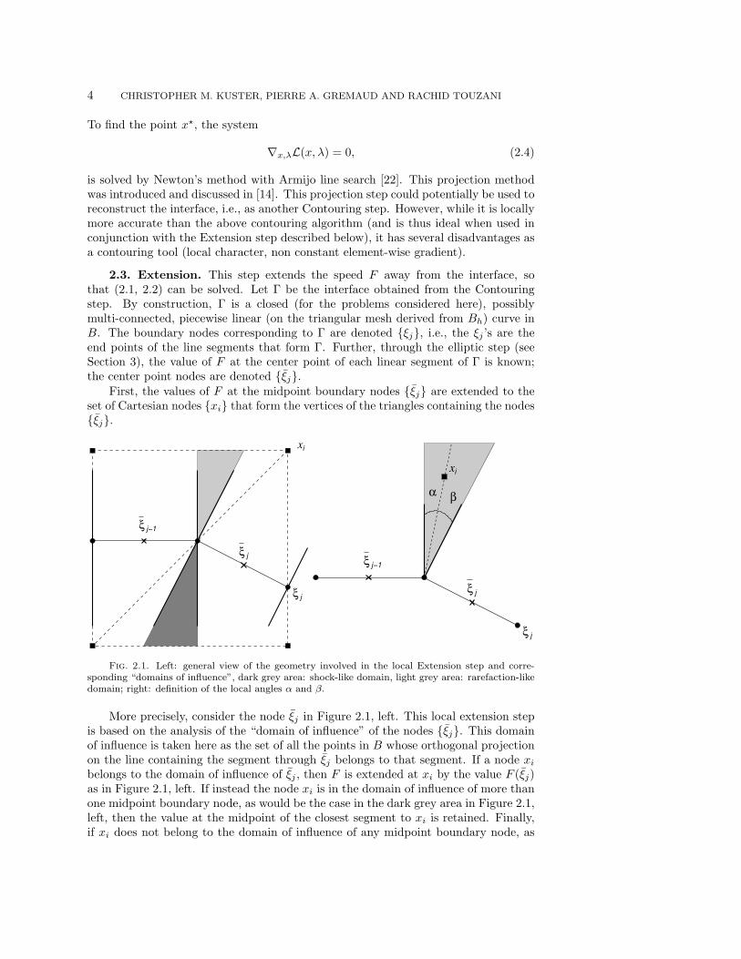
2.3. Extension. This step extends the speed F away from the interface, sothat (2.1, 2.2) can be solved. Let Γ be the interface obtained from the Contouringstep. By construction, Γ is a closed (for the problems considered here), possiblymulti-connected, piecewise linear (on the triangular mesh derived from Bh) curve inB. The boundary nodes corresponding to Γ are denoted ξj, i.e., the ξj ’s are theend points of the line segments that form Γ. Further, through the elliptic step (seeSection 3), the value of F at the center point of each linear segment of Γ is known;the center point nodes are denoted ξj.

First, the values of F at the midpoint boundary nodes ξj are extended to theset of Cartesian nodes xi that form the vertices of the triangles containing the nodesξj.

ξ

ξ

i

j

j

x

ξ j−1

ξ

ξ

j

j

ξ j−1

xi

α β

Fig. 2.1. Left: general view of the geometry involved in the local Extension step and corre-sponding “domains of influence”, dark grey area: shock-like domain, light grey area: rarefaction-likedomain; right: definition of the local angles α and β.

More precisely, consider the node ξj in Figure 2.1, left. This local extension stepis based on the analysis of the “domain of influence” of the nodes ξj. This domainof influence is taken here as the set of all the points in B whose orthogonal projectionon the line containing the segment through ξj belongs to that segment. If a node xi

belongs to the domain of influence of ξj , then F is extended at xi by the value F (ξj)as in Figure 2.1, left. If instead the node xi is in the domain of influence of more thanone midpoint boundary node, as would be the case in the dark grey area in Figure 2.1,left, then the value at the midpoint of the closest segment to xi is retained. Finally,if xi does not belong to the domain of influence of any midpoint boundary node, as


in the light grey area in Figure 2.1, right, then the value of F at xi is taken as

F (xj) =β

α + βFj−1 +

α

α + βFj ,

where Fj−1 and Fj are the values of F at the midpoint boundary nodes ξj−1 and ξj

respectively and where the angles α and β are defined as in Figure 2.1, right. Thisway of defining the local extension of F is compatible with the global extension (2.7).

Second, a renormalized function φ is initialized as a signed distance function atthe same Cartesian nodes at which F has just been extended. The Projection step isused to do this.

We emphasize that both of those local extension steps for F and φ only take placeon the nodes adjacent to the interface; the corresponding values are then used as start-ing points for the extension to the rest of the Cartesian nodes. This is accomplishedusing the Fast Marching method [2] to solve

|∇φ | = 1 in B, (2.5)φ = 0 on Γ, (2.6)

∇F · ∇φ = 0 in B, (2.7)F = F on Γ. (2.8)

A fully upwind mixed first/second order discretization of the above equations is ap-plied on the mesh Bh, see [15, 29, 30] for more details.

2.4. Updating the interface. The interface is moved by updating the corre-sponding level-set function through (2.1, 2.2). More precisely, after the Extensionstep, the level-set function φ corresponding to the current interface Γ is a signeddistance function and in particular, |∇φ| = 1. Therefore, (2.1, 2.2) reads here

∂tφ + F = 0,φ(·, 0) = φ.

The update is then trivially computed by taking one forward Euler step

φnew = φ−∆t F , (2.9)

where ∆t = − 12µ . Note that this corresponds to half the optimal time step given by

(1.8); taking the “optimal” value from (1.8) may lead to overshoots in the positionof the interface and may in fact result in slowing down the convergence of the globaliterative process.

2.5. Initial interface. An initial guess of the interface’s position, ∂A0, needsto be provided. This can be done in an ad hoc way. In Section 4, ∂A0 is taken as acurve of constant distance to Ω.

3. Boundary element method. Consider again the problem (1.5-1.7). For thesake of simplicity, the subscript k is dropped in this section. We assume both ∂A and∂Ω to be simple closed curves and let Γ = ∂A ∪ ∂Ω. The region of interest A \ Ωbeing interior to ∂A and exterior to ∂Ω, ∂A is oriented counterclockwise while ∂Ω isclockwise.

Multiplying (1.5) by the fundamental solution G(x, y) := − 12π log |x − y| and

integrating twice by parts leads to

u(x) =∫

Γ

G(x, y)∂u

∂ny(y) ds(y)−

∫Γ

∂G

∂ny(x, y)u(y) ds(y), (3.1)


where n is the unit outer normal to A \ Ω at y. The above integral representationis valid for x ∈ A \ Ω. To treat the case x ∈ Γ, we define the linear operatorL : L2(Γ) → L2(Γ) by

Lv(x) =

v(x)

2 +∫

∂A∂G∂ny

(x, y) v(y) ds(y)−∫

∂ΩG(x, y) v(y) ds(y) for x ∈ ∂A,∫

∂A∂G∂ny

(x, y) v(y) ds(y)−∫

∂ΩG(x, y) v(y) ds(y) for x ∈ ∂Ω,

and the function F ∈ L2(Γ)

F(x) =

µ

∫∂A

G(x, y) ds(y)−∫

∂Ω∂G∂ny

(x, y) ds(y) for x ∈ ∂A,

µ∫

∂AG(x, y) ds(y)−

∫∂Ω

∂G∂ny

(x, y) ds(y)− 12 for x ∈ ∂Ω.

Taking into account the boundary conditions (1.6) and (1.7), it is then standard tocheck that if

w(x) =

u(x) for x ∈ ∂A,∂u∂n (x) for x ∈ ∂Ω,

where u is the solution to (1.5-1.7) then

Lw(x) = F(x), ∀x ∈ Γ. (3.2)

Problem (3.2) is discretized as follows. The interface ∂A = ∂Ah is obtainedthrough contouring of a given level-set function, see Section 2 and piecewise constantelements are considered. The function w solution to (3.2) is approximated by wh suchthat

wh(x) = we ∀x ∈ e,

where e is an edge of either ∂Ah or ∂Ωh. Equation (3.2) is then collocated at themidpoints of the edges. In other words, for a generic piecewise constant function vh,we define

Lhvh(ξe) =

ve

2 +∫

∂Ah

∂G∂ny

(ξe, y) vh(y) ds(y)−∫

∂ΩhG(ξe, y) vh(y) ds(y) for ξe ∈ ∂Ah,∫

∂Ah

∂G∂ny

(ξe, y) vh(y) ds(y)−∫

∂ΩhG(ξe, y) vh(y) ds(y) for ξe ∈ ∂Ωh,

where ξe is the midpoint of the edge e. Similarly, we also have

Fh(ξe) =

µ

∫∂Ah

G(ξe, y) ds(y)−∫

∂Ωh

∂G∂ny

(ξe, y) ds(y) for ξe ∈ ∂Ah,

µ∫

∂AhG(ξe, y) ds(y)−

∫∂Ωh

∂G∂ny

(ξe, y) ds(y)− 12 for ξe ∈ ∂Ωh.

The approximate solution wh is the solution to

Lhwh(ξe) = Fh(ξe), ∀ξe ∈ ∂Ah ∪ ∂Ωh. (3.3)

The above integrals are computed exactly in the present implementation.Both the integral equation (3.2) and the linear problem (3.3) are well conditioned.

It can be verified that Lh admits eigenvalues and singular values that are boundedindependent of the mesh, see e.g. [17] or [26] for explicit expressions of the eigenvaluesin some specific cases. Further, in spite of the fact that the elements of ∂Ah are allowed


to be arbitrarily small, the condition number of Lh has been numerically verified tobe of order N which would correspond to the uniform mesh case [3]. The conditionnumber of the matrices corresponding to the numerical tests of Section 4 are on theorder of 100. The resulting linear system is solved by GMRES [22, 27] which isconsequently expected to perform well here even without preconditioning. GMRESis restarted after 20 steps (i.e., the solver is GMRES(20)) and is stopped on smallrelative residuals, more precisely the stopping criterion is

‖Fh − Lhw‖2 ≤ 10−10‖Fh‖2,

where w denotes the current iterate. With the above parameters, GMRES has beenobserved to perform slightly better than other CG-like methods such as QMR andBi-CGSTAB [22] on the test problems of Section 4.

4. Numerical results.

4.1. Algorithm. To solve the External Bernoulli problem, we use the followingalgorithm:

Input: a discretization of the boundary ∂Ω, ∂Ωh, µCreate the underlying Cartesian grid Bh

Create a level set function φ on Bh corresponding to ∂A0

k = 0R−1 = 1010 (initial residual)loop

Contour φ (subsection 2.1) to find ∂Ak

Solve (3.3) to get uRk = max of |u| on ∂Ak

if (Rk−1−Rk)/Rk < 10−3 (small residual decrease) thenSTOP

end ifSet F = u on ∂Ak

Extend φ and F (subsections 2.2 and 2.3)Move boundary (subsection 2.4)k = k + 1

end loop

Several remarks are in order.• Progressive mesh refinement can be considered, i.e., a coarse mesh solution

can be used as starting point. A strategy of this type is for instance used in[20] for a similar type of problems but for a different numerical approach.

• In solving (3.3), the “missing” condition (1.3) can be used when choosing theinitial iterate for GMRES. This results in faster convergence (less GMRESiterates) as the algorithm progresses.

• The extension step through Fast Marching (Subsection 2.3) is done in thewhole computational domain B. The corresponding complexity isO(M2 log M)where M2 is the total number of nodes in the Cartesian grid Bh. A narrowband implementation [2, 31] could be considered to speed up the algorithm.However, the global complexity of the problem would not change since, if thewidth of the band is a constant multiple of ∆x, say n∆x, then by (2.9), ∆tshould be reduced from −1

2µ to a value less than n∆x|F | since the band has to con-


tain the boundary. Fast summation techniques can also be implemented [13]to bring down the cost of solving the linear system (3.3), which accounts formost of the computational cost, from O(N2) with the present implementationto O(N), where N is the number of elements of ∂Ωh. A quasi-optimal globalcomplexity of O(M2) = O(N2) is computationally observed in Section 4.

• Higher order boundary element methods can be used [4]. Second order con-vergence is observed in Section 4 (partially as a result of the solution beingconstant on the outer free boundary). To the authors’ knowledge, the presentwork is one of very few published results regarding the accuracy of a combinedlevel-set boundary element method, see for instance [11].

4.2. Example 1. Following [8], a quick look at the radial case is instructive. LetΩ be the unit ball. We consider the problem (1.1-1.4) with Ω as above and µ = −2.The solution to (1.1-1.3) with A being the ball of radius R centered at the origin is

u(r) = −2 R log r + 1,

expressed in polar coordinates. An iterative process similar to the one above can thenbe considered. Taking (1.8) into account, the k-th step of the algorithm reads

Rk+1 = Rk −Rk log Rk +12, k = 1, 2, . . .

Therefore in the fully radial case, the problem amounts to finding a fixed point to thefunction f(R) = R−R log R + 1

2 . The function f has a unique fixed point R where

R =1

2 W ( 12 )

,

the function W being the Lambert W function4 [7].

0 5 10 1510!5

10!4

10!3

10!2

10!1

k

max

|u| o

n !

A

0 5 10 15 20 25

10!5

10!4

10!3

10!2

10!1

100

k

max

|u| o

n !

A

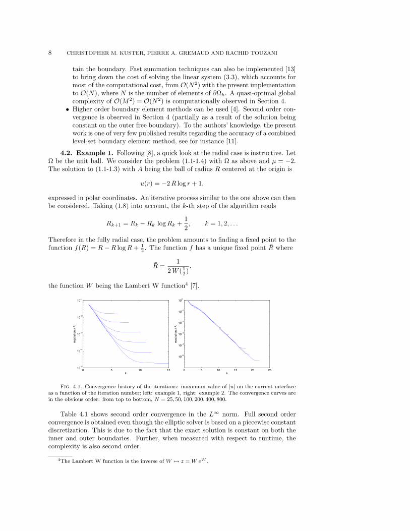
Fig. 4.1. Convergence history of the iterations: maximum value of |u| on the current interfaceas a function of the iteration number; left: example 1, right: example 2. The convergence curves arein the obvious order: from top to bottom, N = 25, 50, 100, 200, 400, 800.

Table 4.1 shows second order convergence in the L∞ norm. Full second orderconvergence is obtained even though the elliptic solver is based on a piecewise constantdiscretization. This is due to the fact that the exact solution is constant on both theinner and outer boundaries. Further, when measured with respect to runtime, thecomplexity is also second order.

4The Lambert W function is the inverse of W 7→ z = W eW .


N max |u| on Γ Rate L∞ Error Rate k Time Rate25 1.64(-2) – 1.53(-2) – 6 0.71 –50 5.07(-3) 1.7 4.40(-3) 1.8 8 4.1 2.5100 1.30(-3) 2.0 1.12(-3) 2.0 10 19 2.2200 3.34(-4) 2.0 2.85(-4) 2.0 11 76 2.0400 8.18(-5) 2.0 7.10(-5) 2.0 12 372 2.1800 1.92(-5) 2.1 1.74(-5) 2.0 14 1465 2.0

Table 4.1Convergence and complexity rates for Example 1 (radial case); N : number of elements on ∂Ωh,

L∞ Error refers to the Hausdorff distance between exact and computed boundaries, k is the numberof nonlinear iterations (see Section 4.1), Time is the runtime in seconds.

The convergence history is instructive. Figure 4.1, left, displays the error (max-imum of |u| on the free boundary) through the iterations. The behavior of the firstiterates is governed by the geometry, see (2.9), and is only weakly dependent on themesh size ∆x. The later iterations during which the fine structure of the boundary isdetermined do depend on ∆x. This explains the mesh dependency of the number ofiterations observed in Table 4.1.

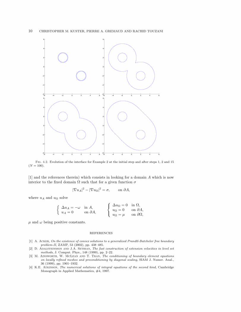
4.3. Example 2. We consider here the problem (1.1-1.4) with Ω consisting oftwo disks of radius 1, one centered at (-2,2), the one at (2,-2); further, µ = −1/4. Theinitial boundary is taken as two circles of radius 1.1, one around each of the innerdisks. Note that for this choice of µ, the exact boundary is simply connected. Acouple of iterates are displayed in Figure 4.2. One can note that after the first stepalready the correct topology of the interface has been achieved.

No exact solution is available for the present example. In Table 4.2, the maximumof u on the boundary is reported. By construction, this maximum should vanish for theconverged solution. The complexity, as measured from the runtimes, is also reported.In both cases, the rates are about two.

N max |u| on Γ Rate k Time Rate26 3.43(-3) – 11 4.4 –50 9.16(-4) 2.0 13 19 2.2100 1.64(-4) 2.5 15 85 2.2200 5.31(-5) 1.6 18 573 2.8400 1.71(-5) 1.6 19 1678 1.6800 4.25(-6) 2.0 21 7613 2.2

Table 4.2Convergence and complexity rates for Example 2; N : number of elements on ∂Ωh, k is the

number of nonlinear iterations (see Section 4.1), Time is the runtime in seconds.

Convergence history is displayed in Figure 4.1, right; a behavior similar as thatof Example 1 is observed.

5. Conclusion. Solutions of the Bernoulli free boundary problem can be effi-ciently computed by the method presented here. Providing a Green’s function is avail-able, the method can be used to solve other free boundary problems. For instance, itcan be applied with only minor modifications to the Prandtl-Batchelor problem (see


!6 !4 !2 0 2 4 6!6

!4

!2

0

2

4

6

!6 !4 !2 0 2 4 6!6

!4

!2

0

2

4

6

!6 !4 !2 0 2 4 6!6

!4

!2

0

2

4

6

!6 !4 !2 0 2 4 6!6

!4

!2

0

2

4

6

Fig. 4.2. Evolution of the interface for Example 2 at the initial step and after steps 1, 2 and 15(N = 100).

[1] and the references therein) which consists in looking for a domain A which is nowinterior to the fixed domain Ω such that for a given function σ

|∇uA|2 − |∇uΩ|2 = σ, on ∂A,

where uA and uΩ solve∆uA = −ω in A,uA = 0 on ∂A,

∆uΩ = 0 in Ω,uΩ = 0 on ∂A,uΩ = µ on ∂Ω,

µ and ω being positive constants.

REFERENCES

[1] A. Acker, On the existence of convex solutions to a generalized Prandtl-Batchelor free boundaryproblem-II, ZAMP, 53 (2002), pp. 438–485.

[2] D. Adalsteinsson and J.A. Sethian, The fast construction of extension velocities in level setmethods, J. Comput. Phys., 148 (1999), pp. 2–22.

[3] M. Ainsworth, W. McLean and T. Tran, The conditioning of boundary element equationson locally refined meshes and preconditioning by diagonal scaling, SIAM J. Numer. Anal.,36 (1999), pp. 1901–1932.

[4] K.E. Atkinson, The numerical solutions of integral equations of the second kind, CambridgeMonograph in Applied Mathematics, #4, 1997.


[5] F. Bouchon, S. Clain and R. Touzani, Numerical solution of the free boundary Bernoulliproblem using a level set formulation, Comp. Meth. Appl. Mech. and Eng., 194 (2005),pp. 3934-3948.

[6] A.J. Chorin and J.E. Marsden, A mathematical introduction to fluid mechanics, Springer,1992.

[7] R.M. Corless, G.H. Gonnet, D.E.G. Hare, D.J. Jeffrey and D.E. Knuth, On the LambertW function, Adv. Comput. Math., 5 (1996), pp. 329–359.

[8] M. Flucher and M. Rumpf, Bernoulli’s free-boundary problem, Qualitative theory and numer-ical approximation, J. Reine Angew. Math., 486 (1997), pp. 165–204.

[9] K.O. Friedrichs, Uber ein Minimumproblem fur Potentialstromungen mit freiem Rand, Math.Ann., 109 (1934), pp. 60–82.

[10] P.R. Garabedian, Calculation of axially symmetric cavities and jets, Pacific J. Math., 6 (1956),pp 611-684.

[11] M. Garzon, D. Adalsteinsson, L. Gray and J.A. Sethian, A coupled level set-boundaryintegral method for moving boundary simulations, Interfaces Free Bound., 7 (2005), pp. 277–302.

[12] R. Gonzalez and R. Kress, On the treatment of a Dirichlet-Neumann mixed boundary valueproblem for harmonic functions by an integral equation method, SIAM J. Math. Anal., 8(1977), pp 504–517.

[13] A. Greenbaum, L. Greengard and G.B. McFadden, Laplace’s equation and the Dirichlet-Neumann map in multiply connected domains, J. Comput. Phys, 105 (1993), pp. 267–278.

[14] P.A. Gremaud, C.M. Kuster and Zhilin Li, A Study of Numerical Methods for the Level SetApproach, NCSU-CRSC Tech Report CRSC-TR05-39, submitted to Appl. Num. Math.

[15] P.A. Gremaud and C.M. Kuster, Computational study of fast methods for the Eikonal equa-tion, SIAM J. Sci. Comput, 27 (2006), pp. 1803-1816.

[16] J. Haslinger, T. Kozubek, K. Kunisch and G. Peichl, Shape optimization and ficticiousdomain approach for solving free-boundary problems of Bernoulli type, Comput. Optim.Appl., 26 (2003), pp. 231–251.

[17] J. Hayes and R. Kellner, The eigenvalue problem for a pair of coupled integral equationsarising in the numerical solution of Laplace’s equation, SIAM J. Appl. Math., 22 (1972),pp. 503–513.

[18] A. Henrot and H. Shahgholian, Existence of classical solutions to a free boundary problemfor the p-Laplace operator: (I) the exterior convex case, J. reine angew. Math., 521 (2000),pp. 85–97.

[19] A. Henrot and H. Shahgholian, The one phase free boundary problem for the p-laplacian withnon-constant Bernoulli boundary condition, Trans. Amer. Math. Soc., 354 (2002), pp. 2399–2416.

[20] K. Ito, K. Kunisch and G.H. Peichl, Variational approach to shape derivatives for a class ofBernoulli problems, J. Math. Anal. Appl. 314 (2006), pp. 126–149.

[21] K.T. Karkkainen and T. Tiihonen, Free surfaces: shape sensitivity analysis and numericalmethods, Int. J. Numer. Engng., 44 (1999), pp. 1079–1098.

[22] C.T. Kelley, Iterative methods for linear and nonlinear problems, Frontiers in Applied Math-ematics #16, SIAM, 1995.

[23] G. Mejak, Numerical solution of Bernoulli-type free boundary value problems by variable do-main method, Int. J. Numer. Meth. Engng., 37 (1994), pp. 4219–4245.

[24] S.J. Osher and R.P. Fedkiw, Level set methods and dynamic implicit surfaces, Applied Math-ematical Sciences #153, Springer, 2002.

[25] S. Osher and J. Sethian, Fronts propagating with curvature dependent speed: algorithms basedon Hamilton-Jacobi formulations, J. Comput. Phys., 56 (1988), pp. 12–49.

[26] G.J. Rodin and O. Steinbach, Boundary element preconditoners for problems defined in slen-der domains, SIAM J. Sci. Comput., 24 (2003), pp. 1450–1464.

[27] Y. Saad and M. Schultz, GMRES a generalized minimal residual algorithm for solving non-symmetric linear systems, SIAM J. Sci. Statist. Comput., 7 (1986), pp. 856–869.

[28] J.A. Sethian, Level Set Methods and Fast Marching Methods, Cambridge University Press(1999).

[29] J.A. Sethian and A. Vladimirsky, Fast methods for the Eikonal and related Hamilton-Jacobiequations on unstructured meshes, Proc. Natl. Acad. Sci. USA, 97 (2000), pp. 5699–5703.

[30] J.A. Sethian and A. Vladimirsky, Ordered upwind methods for static Hamilton-Jacobi equa-tions: theory and algorithms, SIAM J. Numer. Anal., 41 (2003), pp. 325–363.

[31] L. Yatziv, A. Bartesaghi and G. Sapiro, O(N) implementation of the fast marching algo-rithm, J. Comput. Phys., 212 (2006), pp. 393-399.

fast numerical methods for bernoulli free … · fast numerical methods for bernoulli free boundary...

Documents