Fast Track Authorityand International Trade Negotiations∗

Paola Conconi†

Universite Libre de Bruxelles (ECARES) and CEPR

Giovanni FacchiniUniversity of Essex, Universita di Milano, LdA, CEPR and CES-Ifo

Maurizio ZanardiUniversite Libre de Bruxelles (ECARES) and Tilburg University

December 2007

Abstract

Fast Track Authority (FTA) is the institutional procedure in the Unites States wherebyCongress grants to the President the power to negotiate international trade agreements.Under FTA, Congress can only approve or reject negotiated trade deals, with no possibilityof amending them. In this paper, we examine the determinants of FTA voting decisions andthe implications of this institutional procedure for international trade negotiations. We de-scribe a simple two-country trade model, in which industries are unevenly distributed acrossconstituencies. In the foreign country, trade negotiating authority is delegated to the execu-tive, while in the home country Congress can retain the power to amend trade agreements.We show that representatives of constituencies with higher stakes in import-competingindustries tend to vote against FTA, while representatives of more export-oriented con-stituencies might vote in favor or against, depending on the degree of protectionism of themajority of Congress. Empirical analysis of the determinants of all FTA voting decisionstaken by Congress provides strong support for the predictions of our model. We also showthat lack of FTA tends to skew the outcomes of trade negotiations in favor of the homecountry. This might help to explain why other countries are reluctant to negotiate tradeagreements with the United States in the absence of FTA.

JEL classifications: D72, F13Keywords: Fast Track Authority, Trade Negotiations, Strategic Delegation.

∗Research funding from the FNRS is gratefully acknowledged by Paola Conconi. We wish to thank theparticipants at the 2007 ETSG annual conference in Athens, the 2007 CEPR ERWIT meeting in Kiel, the 2007Fall MWIEG meeting at the University of Michigan, and seminar participants at the Universite Libre de Bruxelles(ECARES), Carleton University, and McGill University for their helpful comments. We are also grateful to EstelleCantillon, Peter Egger, Georg Kirchsteiger, Patrick Legros, Michael Moore, Emanuel Ornelas, Diego Puga, AndreSapir, Cecilia Testa, and Thierry Verdier, for their valuable suggestions and to Christopher Magee and JamesSnyder for their help with the collection of congressional district data.

†Correspondence should be addressed to Paola Conconi, European Center for Advanced Research in Economicsand Statistics (ECARES), Universite Libre de Bruxelles, Avenue F. D. Roosevelt 50, CP 114, 1050 Brussels,Belgium; E-mail: pconconi@ulb.ac.be.

1 Introduction

Fast Track Authority (FTA) is the trade negotiating authority granted by the Congress of the

United States to the President. The crucial feature of this institutional procedure is that, when

the President negotiates trade agreements under FTA, Congress can only approve or reject them,

but cannot amend their content. While congressional and private sector leaders are consulted

throughout the negotiations, the fact that the final agreement is presented to Congress as a

package assures trading partners that any solution they reach with U.S. executive will not be

renegotiated.

Fast track procedures played a crucial role during the Tokyo Round and the Uruguay Round

of multilateral trade negotiations, as well as in the negotiations of all major free trade agreements

involving the Unites States.1 The recent expiration of FTA on July 1, 2007 is likely to endanger

the already troubled Doha Round of multilateral trade negotiations,2 as well as ongoing bilateral

negotiations between the Unites States and various other countries. The objective of this paper

is to examine the determinants of congressmen’s decision to grant or not fast track authority

to the President and to understand the impact of this decision on the outcome of international

trade negotiations.

For this purpose, we develop a simple model of trade relations between two large countries,

home (representing the Unites States) and foreign, which are characterized by similar economic

features, but different trade policy institutions. In the foreign country, the authority to negotiate

trade agreements is delegated to the executive, while in the home country, Congress can retain

the possibility to amend trade deals. Each legislator in the home Congress will vote for or

against FTA so as to maximize his expected utility, anticipating the impact that FTA (or lack

thereof) will have on the outcome of the negotiations with the foreign country. We argue that

this decision is effectively equivalent to choosing between two different country representatives:

the President (in the case of FTA) and the majority of Congress (in case of no FTA). Hence the

choice of fast track procedures will only have an impact on trade negotiations if the preferences

of the President do not coincide with those of the majority of Congress.

In our setup, the executive represents the interests of all electoral constituencies in the coun-

try, while congressmen represent only their own electoral constituencies. For fast track to matter,

legislators must have different trade policy preferences, implying that the majority of Congress

and the President have different interest in trade negotiations. We assume that legislators’ trade

1The only free trade agreement which the Unites States did not negotiate under fast track authority wasthe U.S.-Jordan free trade agreement. As stated by Jagdish Bhagwati in a recent interview with the Council ofForeign Relations, “every time there’s been something big and complicated—certainly the big multilateral ones,and even the big bilateral ones like NAFTA—they had to go through fast track” (see www.cfr.org).

2The director-general of the World Trade Organization, Pascal Lamy, warned that the Doha Round “will failunless we get some sort of extension to the fast track” (Sunday Telegraph, December 3, 2006).

1

preferences differ as a result of the uneven distribution of production activities across constituen-

cies. This implies that electoral districts which are relatively more specialized in the production

of import-competing (export) goods will be less (more) willing to trade off reductions in domestic

import tariffs with reductions in foreign import taxes compared to the country as a whole.

Our theoretical model predicts that representatives of constituencies with higher stakes in

import-competing industries will tend to vote against FTA, while representatives of more export-

oriented constituencies may vote in favor or against, depending on the degree of protectionism

of the majority of Congress. The intuition behind this result is that more export-oriented

constituencies, which are eager to reach an agreement with the foreign country, may gain from

being represented by more protectionist constituencies, which are able to achieve a more favorable

deal in the negotiations. This is in line with results obtained in the literature on strategic

delegation, which shows how principals may gain by delegating decision-making power to status

quo-biased agents, to increase their “bargaining power” in negotiations with other parties (e.g.

Schelling, 1956; Jones, 1989; Segendorf, 1998).

We also show that lack of FTA tends to impede trade liberalization and to skew trade policy

outcomes in favor of the home country. This result can explain why foreign countries are reluctant

to negotiate trade agreements with the United States in the absence of FTA.

To test the predictions of our theoretical model concerning FTA voting decisions, we examine

the determinants of all FTA votes which have taken place in the U.S. Congress between 1974

(when fast track was first introduced) and 2002 (when it was last granted). Our results provide

strong empirical support for the voting predictions of our model. In particular, we show that a

congressman is significantly less likely to vote in favor of granting or extending FTA the more

his constituency is specialized in import-competing production compared to the entire country.

Moreover, in line with the predictions of our theoretical model, the FTA voting decisions of less

protectionist district representatives depend crucially on the characteristics of Congress majority.

Our analysis builds on the broad literature on the political economy of trade policy, and in

particular on the various contributions which have examined the interaction between domestic

politics and trade negotiations (e.g. Mayer, 1981; Grossman and Helpman, 1995; Broda et

al., 2007). While these papers have considered several important aspects of the process of

endogenous formation of trade policies, somewhat surprisingly, very little attention has been

paid by the literature to the workings of FTA and and its impact on trade negotiations. The

idea that negotiators may use various strategies to try to shift the terms of the agreements closer

to their own preferred outcome was informally discussed by Putnam (1988), who was the first

to describe international relations as “two-level games”, in which domestic and international

politics are fundamentally intertwined.

Our paper is also related to the vast literature in political science that has examined the

2

evolution of U.S. trade policy institutions (e.g. Lohmann and O’Halloran, 1994; Bailey et al.,

1997; Hiscox, 1999).3 To the best of our knowledge, this is the first paper to focus on FTA, pro-

viding a fully microfounded theoretical model to understand the determinants of this institution

and its impact on U.S. trade relations. Finally, our paper contributes to the empirical literature

which has examined the determinants of congressional trade policy decisions (e.g. Kahane, 1996;

Box-Steffenmeier et al., 1997; Baldwin and Magee, 2000a,b).4

The remainder of the paper is organized as follows. In Section 2, we present a brief history of

fast track authority. In Section 3, we develop a simple model of trade negotiations between two

large countries (home and foreign). Section 4 introduces the trade policy preferences of Congress

representatives in the home country, examines the determinants of FTA voting behavior and the

implications for trade negotiations. Sections 5 describes the data used in our empirical analysis,

while Section 6 presents our methodology and our results. Section 7 reports the results of various

robustness checks. Finally, Section 8 concludes, discussing the implications of our analysis for

institution design.

2 A Brief History of Fast Track Authority

The U.S. Constitution explicitly assigns authority over foreign trade to Congress. Article I,

section 8, gives Congress the power to “regulate commerce with foreign nations ...” and to

“...lay and collect taxes, duties, imposts, and excises...”. Under Article II, however, the President

is granted exclusive authority to negotiate treaties and international agreements and exercises

broad authority over the conduct of the nation’s foreign affairs. Hence, both legislative and

executive authorities have a role to play in the development and execution of U.S. trade policy.

For roughly the first 150 years of the United States, Congress exercised its authority over

3Most of these studies have focused on the impact of the Reciprocal Trade Agreements Act (RTAA) of 1934.As discussed in Section 2, this was the first bill in which Congress delegated trade policy to the President.Lohmann and O’Halloran (1994) present a theoretical model of distributive politics in which legislators delegatepolicymaking to the President to avoid being trapped in inefficient logrolling. Their analysis cannot be appliedto understand the implications of fast track authority on trade negotiations, since it focuses only on one country.Bailey et al. (1997) use a spatial model to show how reciprocity in trade agreements can help to solve the collectiveaction problems of exporters. Notice that in their analytical framework, the preferences of the legislators aresimply assumed rather than being derived from a fully microfounded trade model. Similarly to our analysis,Hiscox (1999) models trade policy decisions in Congress as being shaped by differences in the endowments ofspecific factors across constituencies; however, his analysis is focused only on one country, and thus cannot beapplied to examine how trade policy delegation affects strategic interaction between countries.

4In this literature, the paper which is closest to ours is Baldwin and Magee (2000a), who examine the de-terminants of three votes taken by Congress in 1993-1994 (on NAFTA, the Uruguay Round Agreement, andthe most-favored nation status to China). Similarly to our analysis, they find legislators’ voting behavior to beaffected by the extent to which their constituencies depend on jobs in export sectors relative to jobs in import-competing sectors, as well as by other factors (e.g. the ideology of the legislators, their party affiliation, and thelobbying contributions they receive).

3

foreign trade by setting tariff rates on all imported products. Tariffs were the main trade

policy instrument and a primary source of federal revenues. During this period, the President’s

primary role in setting trade policy was in negotiating and implementing bilateral trade treaties

with the advice and consent of Congress. In the 1930’s, two legislative events radically changed

the shape and conduct of U.S. trade policy. The first was the infamous Smoot-Hawley Act,

which raised import duties to record levels and was widely blamed at the time for sharply

reducing trade, triggering retaliatory moves by many other countries, and exacerbating the

Great Depression (see Irwin, 1997). The second important piece of legislation was the Reciprocal

Trade Agreements Act (RTAA) of 1934, which gave the President the authority to undertake

tariff-reduction agreements with foreign countries. The crucial feature of the RTAA was that the

President could implement trade agreements by proclamation, i.e., with no need for congressional

approval, although the RTAA itself required periodic renewal. The idea behind the RTAA was

to undo the damage created by Smoot-Hawley, unwinding beggar-thy-neighbor trade policies

through negotiated tariff reductions. Under the authority of the RTAA, the executive reached

numerous bilateral trade agreements in the late 1930s and negotiated the General Agreement on

Tariffs and Trade (GATT) in 1947.

Under the Trade Expansion Act of 1962, Congress granted again RTAA authority for five

years. This allowed the President to negotiate the Kennedy Round (1963-1967), in which GATT

members reached an agreement on a number of tariff reductions. However, since this agree-

ment also involved interventions in two areas related to non-tariff barriers (customs valuation

and antidumping practices), some congressmen argued that the President had overstepped his

authority. The outcome of the Kennedy Round made evident that non-tariff barriers would

increasingly dominate the agenda of future trade negotiations. As a result, when Congress con-

sidered a new grant of authority for the Tokyo Round of GATT negotiations, it decided to

maintain final control over non-tariff agreements.

The process ultimately agreed upon in the Trade Act of 1974 is what is known as “fast

track”. Three key features characterize this institutional procedure. First, the act stipulates that

agreements involving non-tariff barriers cannot enter into force by presidential proclamation, but

need to be approved by Congress. Second, under fast track authority, Congress cannot amend

a trade agreement once it has been submitted for approval.5 Finally, the Trade Act of 1974

requires Congress to consider trade agreement implementing bills within mandatory deadlines

5During the drafting of the Trade Act of 1974, it was recognized that trading partners would be unwilling tonegotiate agreements that would be subject to unlimited congressional debate and amendments. As stated inthe Senate Finance Committee report accompanying the legislation: “The Committee recognizes ... that suchagreements negotiated by the Executive should be given an up-or-down vote by the Congress. Our negotiatorscannot be expected to accomplish the negotiating goals ... if there are no reasonable assurances that the negotiatedagreements would be voted up-or-down on their merits. Our trading partners have expressed an unwillingness tonegotiate without some assurances that the Congress will consider the agreements within a definite time-frame.”

4

-

1974 1979 1988 1991 1993 1998 2002

Fta granted

︷ ︸︸ ︷Ford

︷ ︸︸ ︷Carter

︷ ︸︸ ︷Reagan

︷ ︸︸ ︷︷ ︸︸ ︷ ︷ ︸︸ ︷G.Bush Clinton G.W.Bush

Fta granted

2007

Figure 1: Conferrals of FTA

and with a limitation on debate.6

Additional provisions of the Trade Act of 1974 involve restrictions on the President’s powers

under FTA. In particular, in his request for trade negotiating authority the executive must

specify what types of agreements it will be used for and what his negotiating objectives will

be. Furthermore, he has to consult with Congress during the course of the negotiations and

during the drafting of the implementing legislation. Finally, Congress sets a deadline by which

the negotiations have to be completed if fast-track procedures are to apply.7

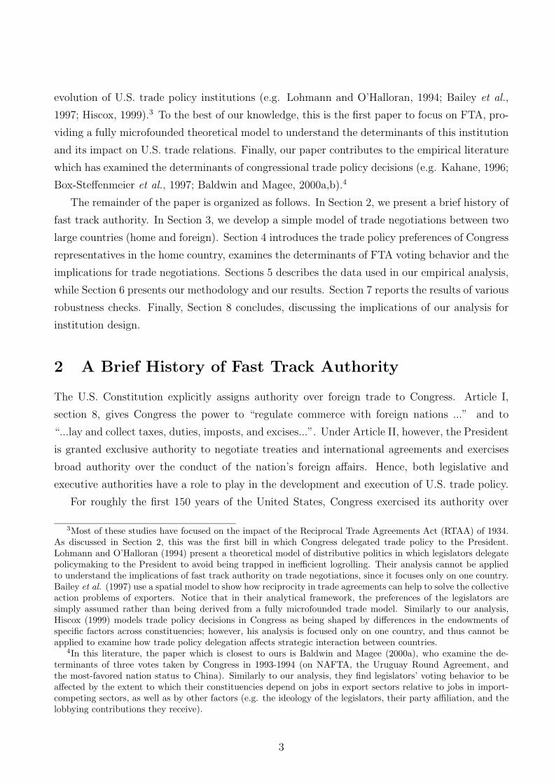
Table 1 reports the outcome of all the votes in which Congress decided to authorize or

extend fast track authority. Notice that some of the listed bills focus solely on fast track trade

negotiating authority, while others include other trade provisions. The only episode of denial of a

FTA request is represented by H.R. 2621 of September 25, 1998, when the Clinton administration

was defeated by a 243 to 180 majority.

Figure 1 above illustrates the periods in which FTA has been granted since the Trade Act of

1974. As it can be seen, every President has enjoyed FTA, with the exception of Bill Clinton,

who failed to obtain it between 1994 and 2001. Notice also that FTA has been granted for

periods of different length and has often spanned more than one presidency.

¿From Table 2 below, we can see that all the most important multilateral and preferential

trade agreements signed by the United States have been negotiated under fast track procedures.

Presidential fast track trade negotiating authority, renamed “trade promotion authority” by the

George W. Bush administration, was last renewed with the Trade Act of 2002. This allowed the

United Stated to implement several free trade agreements with countries such as Australia and

Chile and to negotiate four additional bilateral trade deals with Peru, Panama, South Korea

6Each house can debate the bill for no more than 20 hours. The entire Congressional consideration can takeno longer than 90 legislative days.

7See Destler (1997), Brainard and Shapiro (2001), and Smith (2007) for a more detailed description on fasttrack procedures.

5

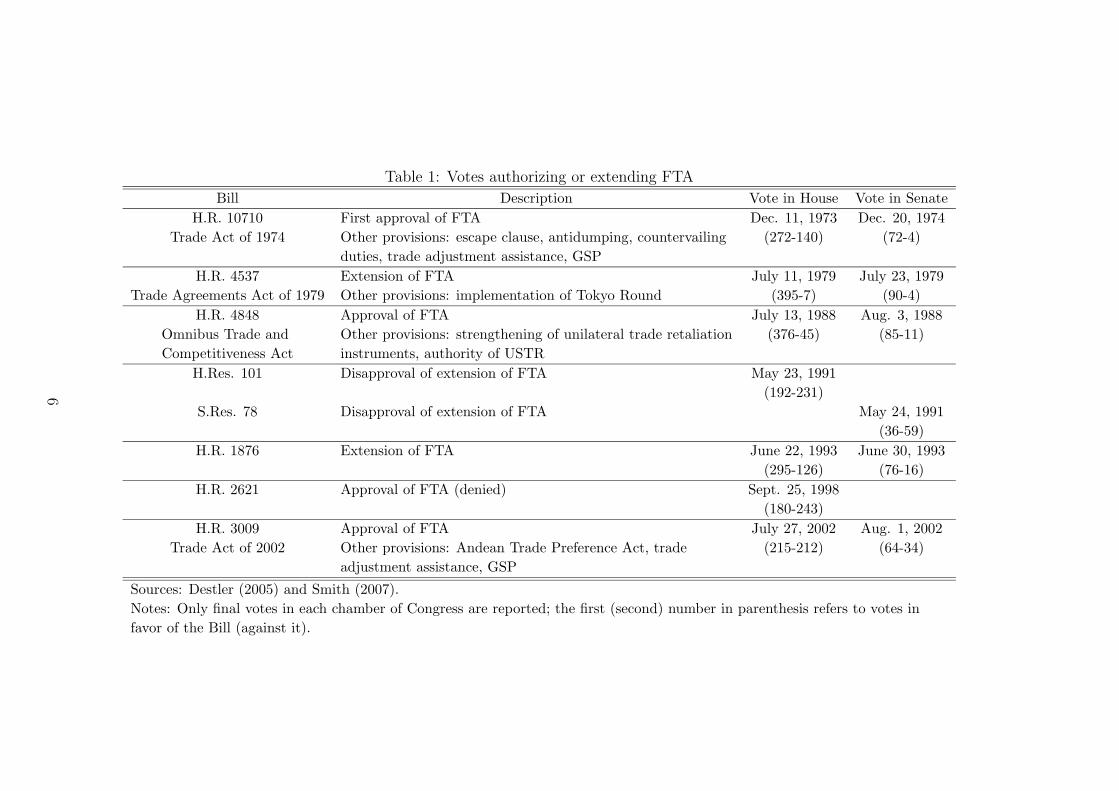
Table 1: Votes authorizing or extending FTA

Bill Description Vote in House Vote in Senate

H.R. 10710 First approval of FTA Dec. 11, 1973 Dec. 20, 1974

Trade Act of 1974 Other provisions: escape clause, antidumping, countervailing (272-140) (72-4)

duties, trade adjustment assistance, GSP

H.R. 4537 Extension of FTA July 11, 1979 July 23, 1979

Trade Agreements Act of 1979 Other provisions: implementation of Tokyo Round (395-7) (90-4)

H.R. 4848 Approval of FTA July 13, 1988 Aug. 3, 1988

Omnibus Trade and Other provisions: strengthening of unilateral trade retaliation (376-45) (85-11)

Competitiveness Act instruments, authority of USTR

H.Res. 101 Disapproval of extension of FTA May 23, 1991

(192-231)

S.Res. 78 Disapproval of extension of FTA May 24, 1991

(36-59)

H.R. 1876 Extension of FTA June 22, 1993 June 30, 1993

(295-126) (76-16)

H.R. 2621 Approval of FTA (denied) Sept. 25, 1998

(180-243)

H.R. 3009 Approval of FTA July 27, 2002 Aug. 1, 2002

Trade Act of 2002 Other provisions: Andean Trade Preference Act, trade (215-212) (64-34)

adjustment assistance, GSP

Sources: Destler (2005) and Smith (2007).

Notes: Only final votes in each chamber of Congress are reported; the first (second) number in parenthesis refers to votes in

favor of the Bill (against it).

6

Table 2: Bills negotiated under FTA

Bill Status Votes/Signature Date

Trade Agreement Act of 1979 Approved Tokyo Round Agreements July 1979

U.S.-Israel Free Trade Area Approved free trade area May 1985

U.S.-Canada Free Trade Area Approved free trade area Aug./Sept. 1988

NAFTA Approved free trade area between Nov. 1993

United States, Canada and Mexico

Uruguay Round Approved Uruguay Round Agreements Nov./Dec. 1994

U.S.-Chile Free Trade Area Approved free trade area July 2003

U.S.-Singapore Free Trade Area Approved free trade area July 2003

U.S.-Australia Free Trade Area Approved free trade area July 2004

U.S.-Morocco Free Trade Area Approved free trade area July 2004

U.S.-Dominican Republic-Central Approved free trade area between July 2005

America Free Trade Area United States, Dominican Republic,

Costa Rica, El Salvador, Honduras,

Guatemala, and Nicaragua

U.S.-Bahrain Free Trade Area Approved free trade area Dec. 2005

U.S.-Oman Free Trade Area Approved free trade area July/Sept. 2006

U.S.-Peru Free Trade Area Approved free trade area Nov./Dec. 2007

U.S.-Colombia Free Trade Area Awaiting congressional approval November 2006

U.S.-Panama Free Trade Area Awaiting congressional approval June 2007

U.S.-South Korea Free Trade Area Awaiting congressional approval June 2007

and Colombia.

FTA expired on July 1, 2007 and has yet to be renewed. Without renewal of fast track, it

has been argued that the current administration has “diminished leverage to pursue additional

trade deals, and the prospects for completion of the Doha Round of global trade talks, as well as

several proposed bilateral U.S. trade deals, remain bleak” (Wall Street Journal, June 29, 2007).8

3 A Simple Model of Trade Negotiations

To analyze the working of FTA, we introduce a standard model of trade relations between two

large countries, “home” and “foreign” (represented by a “*”). We focus on countries char-

acterized by similar economic structures, in which trade is the result of differences in factor

endowments. Each country is made up of several electoral constituencies, which differ with

respect to their stakes in import-competing and export industries.

In this section, we examine international negotiations between the executives of the two

8It is still not clear how the expiration of fast track will affect the outstanding bilateral trade pacts with Peru,Panama, South Korea and Colombia. Some claim that, since these agreements have been negotiated before theexpiration deadline, they should be considered by Congress under fast track procedures. Others argue insteadthat a renewal of FTA is necessary (see Smith, 2007).

7

countries, who are assumed to represent the interests of all constituencies and to have full

control over trade policy. The core of our analysis is presented in the following section, in which

we allow legislators in the home country to choose whether or not to delegate trade negotiating

authority to the President.

Each economy is characterized by three sectors, i = 0, 1, 2, where 0 denotes a numeraire

good. The numeraire good is traded freely across countries and is produced using labor alone.

We choose units so that the international and domestic price of good 0 are both equal to one. We

assume that aggregate labor supply, L = L∗, is large enough to sustain production of a positive

amount of good 0. This implies that in a competitive equilibrium the wage rate equals unity in

each country.

Goods 1 and 2 are manufactured using labor and a sector-specific input, which is available

in fixed supply. Home is abundant in sector-specific input 2, while foreign is abundant in sector-

specific input 1. As a result, home imports good 1, while foreign imports good 2. We will assume

perfect symmetry in the factor endowments between the two countries.

The domestic and international price of a nonnumeraire good i are denoted by pi and πi,

respectively. With a wage rate equal to unity, the total rent Ri accruing to the specific factor in

sector i depends only on the producer price of the good, and can thus be expressed as Ri(pi).

Industry supply is given by Qi(pi) = ∂Ri/∂pi.

Trade policies in the two countries consist of ad valorem import tariffs or subsidies, denoted

by τ and τ ∗, which drive a wedge between domestic and international prices. In the home

country, the domestic price of good 1 is thus equal to p1 = (1 + τ)π1, with τ > 0 (τ < 0)

representing an import tariff (subsidy); the domestic price of the export good is instead equal

to p2 = π2. In the foreign country, domestic prices are given by p∗1

= π1 and p∗2

= (1 + τ ∗)π2.9

The economy is populated by a continuum of agents, and the population size is normalized

to one. Each agent in [0, 1] is indexed by h and shares the same, quasi-linear and additively

separable preferences, which can be written as

uh(c0, c1, c2) ≡ c0 +2∑

i=1

ui(ci), (1)

where c0 represents the consumption of the numeraire good, and c1 and c2 represent the con-

sumption of nonnumeraire goods. The utility functions are assumed to be twice differentiable,

increasing, and strictly concave.

9Following Johnson (1953-4) and Mayer (1981), we restrict the set of policy tools available to import tariffsand subsidies. This allows us to describe the preferences of the two countries in the tariff space (τ , τ∗) and toeasily characterize trade negotiations between them. Levy (1999), in his model of lobbying and internationalcooperation, has convincingly argued that export subsidies and taxes are rarely used, the only exception beingprobably agriculture (see also Hoeckman and Kostecki, 2001).

8

Provided that income always exceeds the expenditure on the numeraire good, the domestic

demand for good i ∈ 1, 2 can be expressed as a function of price alone, Di(pi). Net imports of

good 1 by the home country can then be written as M1(p1) = D1(p1)−Q1(p1) > 0, while foreign

net imports are given by M∗

1(p∗

1) = D∗

1(p∗

1)−Q∗

1(p∗

1) < 0. World product markets of goods 1 and

2 clear when

M1

(

(1 + τ)π1

)

+ M∗

1(π1) = 0, (2)

M2(π2) + M∗

2

(

(1 + τ ∗)π2

)

= 0. (3)

¿From (2) and (3)we can derive an expression for world equilibrium prices as a function of the

policies in the two countries, i.e., π1(τ), π2(τ∗). Tariff revenues in home are given by

T (t) = τπ1(τ)M1(τ) (4)

and are assumed to be redistributed uniformly to all individuals. The same is true for foreign.

Individuals derive income from various sources: they all own a unit of labor and earn wages

as workers; they also receive the same lump sum transfer (possibly negative) of trade policy

revenues from the government; in addition, some individuals own a share of the specific inputs

used in the production of goods 1 and 2. Aggregate welfare is defined as the sum of the income of

all citizens (total labor income, industry rents and government revenues), plus consumer surplus,

and for the case of home it can then be written as

W (τ , τ ∗) = 1 + R1(τ) + R2(τ∗) + T (τ) + Ω(τ , τ ∗), (5)

where Ω(τ , τ ∗) ≡ u(

D1(τ))

− p1D1(τ) + u(

D2(τ∗)

)

− p2D2(τ∗) denotes total consumer surplus.

The welfare of the foreign country can be defined symmetrically.

Dropping the sectoral subscript for notational simplification, the first-order condition for the

maximization of (5) can be written as10

−Mdπ

dτ+ τπ

dM

dτ= 0. (6)

Substituting the expression for (dπ/dτ) into (6) yields the standard formula for the home coun-

10This is found by substituting −D(dp/dτ) and Q(dp/dτ) for the derivatives of consumer surplus and industryrents, respectively, and by substituting (dp/dτ) = (1 + τ)(dπ/dτ) + π.

9

6

-

W3

W2

W1

τ ∗

τ

Figure 2: Home’s indifference map

try’s optimal import tariff:11

τ =1

ε∗, (7)

where ε∗ ≡ (dM∗/dp∗)(p∗/M∗) is the elasticity of foreign export supply.

Figure 2 illustrates the home country’s indifference map in the tariff plane (τ , τ ∗). Each

indifference curve represents the combinations of domestic (τ) and foreign (τ ∗) tariffs among

which the home country is indifferent. These tariff indifference curves are denoted by WU ,

with welfare increasing as subscript U rises in value. An expression for the slope of the tariff

indifference curves is derived in the Appendix (see equation (21)). There we show analytically

that, for non-negative values of τ , the slope of the home country’s indifference curves is positive,

zero or negative depending on the home country’s actual tariff rate being less than, equal to, or

larger than its optimal tariff.

Similarly, we can characterize the indifference curves of the foreign country (see Appendix for

the derivation). Combining information on the preferences of the two countries, we can examine

the scope for trade agreements between them. In this section, we will focus on the case in which

the authority to negotiate trade agreements in both home and foreign is fully delegated to the

President, who represents the interests of all the constituencies in his country.

In Figure 3 below, we illustrate the scope for trade agreements between the two executives,

11The expression for (dπ/dτ) is derived applying the implicit function theorem to the market-clearing condition(2):

dπ

dτ= −

π dMdp

dMdp

(1 + τ) + dM∗

dp∗

.

10

6

-

τ ∗

τ

WN

W ∗

N

NC

A

B

O

C

Figure 3: Trade negotiations between the two Presidents

taking the noncooperative Nash tariff equilibrium point N , as the status quo point for the

negotiations. Graphically, the tariff war outcome lies at the intersection point between two

indifference curves of the home and foreign executives, such that both indifference curves reach

a maximum at that point.12

We make the following standard assumptions about trade agreements:

Assumption 1 The negotiating parties can only agree to tariff combinations, that make each

of them at least as well off as they would be in a tariff war.

Graphically, this assumption implies that trade agreements must be in the lens comprised be-

tween the two indifference curves going through the Nash equilibrium, WN and W ∗

N . We also

require trade deals to be efficient:

Assumption 2 The negotiating parties can only agree to tariff combinations such that no fur-

ther welfare gains can be achieved by one party without the other one losing.

This assumption implies that agreed tariff combinations must lie on the contract curve (CC in

Figure 3), the locus of all tangency points between the indifference curves of the two countries.

12The diagram shows a unique Nash equilibrium, which is given by the tariff pair (τN , τ∗N ) such that τN is a

best response to τ∗N , and vice versa. In general, multiple equilibria cannot be excluded. See Johnson (1953-4)

for a full characterization of Nash equilibria in tariff games.

11

6

-

O

N

E

W ∗

W

A

B

Figure 4: Bargaining between the two Presidents

In the Appendix, we show that efficient trade deals between the home and foreign country are

characterized by the following condition:

(1 − τǫ∗)(1 − τ ∗ǫ) − 1 = 0. (8)

Equation 8 states that there exists an infinite number of tariff-subsidy combinations for the

two countries, which satisfy Assumption 2. If one country imposes a tariff, the other country must

offer a subsidy. Tariffs in both countries cannot be the outcome of efficient trade negotiations

between the two countries. Free trade is the symmetric efficient outcome.13

Together, the two assumptions above imply that the two parties agree to combinations of

import tariffs (subsidies) which lie on the segment A-B of the contract curve in Figure 3. This

segment identifies all possible trade agreements which satisfy the above two assumptions, i.e.,

they are in the set of Pareto-improving deals compared to the status quo and are efficient.

We can summarize the information in Figure 3 and derive trade negotiation outcomes by

drawing the utility possibility frontier. This is done in Figure 4, where the origin is point N ,

which corresponds to the utility levels in a tariff war, WN and W ∗

N in Figure 3. The curve AB in

Figure 4 represents the utility possibility frontier, which traces the utilities of the two countries

as we move along the corresponding curve AB in Figure 3.

In order to derive the equilibrium outcome of the trade negotiations, we employ the general-

13See Mayer (1981) for a similar result.

12

ized Nash bargaining solution. This implies that the domestic and foreign tariffs τ and τ ∗ must

be chosen so as to solve the following maximization problem:

maxW,W ∗

(W − WN)γ(W ∗ − W ∗

N)1−γ , (9)

where γ ∈ (0, 1) captures the relative bargaining strength of the home government.14 If we

consider the case of two symmetric countries, for which γ = 1

2, the outcome of the negotiations

will be point O in Figure 4, which corresponds to the free trade point O in Figure 3.15 If instead

we increase the bargaining power of the home country, the solution will be a point like E where,

as expected, the stronger bargainer does relatively better than its trading partner. In the limit,

when γ = 1 (γ = 0), the equilibrium utility levels are given by point B (A), where the home

(foreign) country gets the maximum level of utility and the foreign (home) country achieves the

same level of utility as in the Nash equilibrium.

4 FTA and Trade Negotiations

In the analysis developed in the previous section, we have assumed that trade negotiations

between home and foreign were carried out by the two executives, who represent the interests

of the nation at large, i.e., one large district made up by all the electoral constituencies. In this

section, we introduce a crucial asymmetry between the negotiating countries: for foreign, we

retain the assumption that trade policy is set by the President; for home, we assume instead that

the legislators in Congress must decide whether or not to delegate trade negotiating authority to

the President by granting FTA. This allows us to focus on the impact of FTA on the outcomes

of trade negotiations. Later, in Section 8, we discuss the implications of allowing Congress in

both countries to retain amendment power.

The starting point of the political economy model described below is the uneven geographical

distribution of industries across constituencies. This implies that the trade policy preferences

of the members of Congress will be heterogenous, as they reflect the interests of their electoral

districts, which depend on the specific industries located there.16

It should be stressed that the our analysis does not rely on the specific preferences we have

14Notice that the parameter γ does not reflect the countries’ market power or their costs in case of tradenegotiation failure, which are already captured by the utility possibility frontier; as argued by Binmore et al.

(1986), γ could be interpreted instead as reflecting differences in discount rates.15It should be stressed that free trade would arise as the outcome of the negotiations between two symmetric

countries even if we used alternative bargaining solutions (e.g. under utilitarian or egalitarian bargaining).16There is substantial evidence on the importance of geographical industry concentration in trade policy is

pervasive. See, for example, Hansen (1990) and Busch and Reinhardt (1999). Grossman and Helpman (2005)and Willmann (2005) show in a small-country trade model how asymmetries in the distribution of industriesacross constituencies may lead to a protectionist bias in national legislators.

13

assumed for the President and the legislators, but rather on the fact that the executive’s prefer-

ences do not coincide with those of the majority of Congress.

4.1 Congressional Preferences in the Home Country

In the home country, there are D districts, each populated by h = H/D individuals and rep-

resented in Congress by one legislator. Note that, since we have normalized the country’s

population size H to unity, h captures the share of the total population residing in each dis-

trict/constituency. All districts have identical preferences (equation (1) above) and receive the

same transfer from the government. Importantly, districts differ with respect to their stakes in

the production of import-competing and export goods, implying different trade policy prefer-

ences. In particular, we distinguish three types of districts/congressmen:

• Import districts (M): a fraction βM of the D districts is relatively specialized in the

production of the import-competing good. Each of these districts is characterized by a

share αM1

(αM2

) of rents in the production of import (export) goods, with αM1

> αM2

. The

utility function of a representative of one of these districts is thus given by

WM(τ , τ ∗) = h + αM1

R1(τ) + αM2

R2(τ∗

k) + h [T (τ) + Ω(τ , τ ∗)] . (10)

• Export districts(S): a fraction βS of districts is relatively specialized in the production

of export goods. Each of these districts is characterized by a share αS1

(αS2) of the rents

associated with import (export) production, with αS1

< αS2. The utility function of a

representative of one of these districts is given by

W S(τ , τ ∗) = h + αS1R1(τ) + αS

2R2(τ

∗

k) + h [T (τ) + Ω(τ , τ ∗)] . (11)

• Neutral districts (C): the remaining fraction βC = 1−βM −βS of districts has equal stakes

in the production of all goods, i.e., αC1

= αC2

= h. The utility function of a representative

of one of these districts can thus be written as

WC(τ , τ ∗) = h + hR1(τ) + hR2(τ∗

k) + h [T (τ) + Ω(τ , τ ∗)] , (12)

implying that a C district is just a scaled-down representation of the country’s economy.

Equations (10)-(12) above imply that congressional districts have different preferences only due

to the asymmetric distribution of industry rents across them.17 Notice that our formulation

17Notice that this implies an interaction between the size of a group of districts in Congress and the policypreferences of this group. For example, if we increase the share of M districts in Congress by increasing βM ,

14

assumes homogeneous trade preferences within each type of districts (M , S or C), implying

no coordination failure in voting and no role for logrolling. It can be shown, however, that

the results of our analysis would still hold if we allowed for asymmetries within each type of

districts.18

More importantly, asymmetries with respect to the geographic location of production activ-

ities across various districts imply different preferences over trade policy: M , S and C districts

will have different indifference curves, reflecting different trade offs between domestic and foreign

protection.19

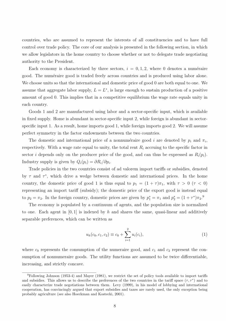
In Figure 5 above we plot the indifference curves of the three types of districts going through

a generic point Z in the tariff space (τ , τ ∗). Notice that the indifference curves of the neutral C

districts have the same shape as those of the benevolent home executive (represented in Figure 2

above). Furthermore, the indifference curves of the representative of an import (export) district

M (S) are steeper (flatter) than the indifference curves of the President (and the C districts).

This reflects the fact that districts that are relatively specialized in the production of import-

competing (export) goods are less (more) willing to trade off a reduction in domestic import

tariffs with a reduction in foreign import taxes. See Appendix for a formal derivation.

4.2 Timing

The main ingredient of the political economy model described above is the uneven geographical

distribution of the endowments of the specific factors used in the production of import-competing

and export goods, implying asymmetries in the trade policy stances of the legislators. In the

home country, Congress will decide whether or not to delegate trade negotiating authority to the

President (granting FTA) or to retain amendment power (not granting FTA). Each legislator

will vote to maximize his expected utility, anticipating the impact that FTA (or lack thereof)

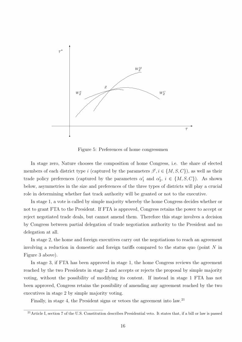
will have on the outcome of the negotiations with the foreign country.20 The game involves five

stages and is illustrated in Figure 6 below.

we must have that each of these districts enjoys a smaller proportion of the rents from the production of theimport-competing good 1. To see this, notice that we must have αM

1βM + αS

1βS + h(1 − βM − βS) = 1/D,

implying∂αM

1

∂βM < 0.18We could extend our trade model to a setting with N nonnumeraire goods, in which each M (S) district is

relatively specialized in the production of one import-competing (export) good. In this setting, different M (S)districts would have different trade policy preferences across sectors, but would gain by coordinating their votesthrough logrolling.

19It could be argued that differences in trade policy stances across legislators would be attenuated in thepresence of compensation mechanisms like the Trade Adjustment Assistance program. The analysis of the role oftransfers is beyond the scope of this paper (see Magee (2001) and Drazen and Limao (fortcoming) on this point).

20Notice that asymmetries across foreign constituencies will play no role in the negotiations, since we assumethat in the foreign country trade negotiation authority is always fully delegated to the President, who representsthe interests of all constituencies.

15

6

6

-

τ ∗

τ

W S

Z

W M

Z

W C

Z

Z

Figure 5: Preferences of home congressmen

In stage zero, Nature chooses the composition of home Congress, i.e. the share of elected

members of each district type i (captured by the parameters βi, i ∈ M,S,C), as well as their

trade policy preferences (captured by the parameters αi1

and αi2, i ∈ M,S,C). As shown

below, asymmetries in the size and preferences of the three types of districts will play a crucial

role in determining whether fast track authority will be granted or not to the executive.

In stage 1, a vote is called by simple majority whereby the home Congress decides whether or

not to grant FTA to the President. If FTA is approved, Congress retains the power to accept or

reject negotiated trade deals, but cannot amend them. Therefore this stage involves a decision

by Congress between partial delegation of trade negotiation authority to the President and no

delegation at all.

In stage 2, the home and foreign executives carry out the negotiations to reach an agreement

involving a reduction in domestic and foreign tariffs compared to the status quo (point N in

Figure 3 above).

In stage 3, if FTA has been approved in stage 1, the home Congress reviews the agreement

reached by the two Presidents in stage 2 and accepts or rejects the proposal by simple majority

voting, without the possibility of modifying its content. If instead in stage 1 FTA has not

been approved, Congress retains the possibility of amending any agreement reached by the two

executives in stage 2 by simple majority voting.

Finally, in stage 4, the President signs or vetoes the agreement into law.21

21Article I, section 7 of the U.S. Constitution describes Presidential veto. It states that, if a bill or law is passed

16

-

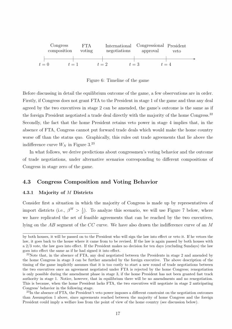
t = 0

Congresscomposition

t = 1 t = 2 t = 3 t = 4

FTAvoting

Internationalnegotiations

Congressionalapproval

Presidentveto

Figure 6: Timeline of the game

Before discussing in detail the equilibrium outcome of the game, a few observations are in order.

Firstly, if Congress does not grant FTA to the President in stage 1 of the game and thus any deal

agreed by the two executives in stage 2 can be amended, the game’s outcome is the same as if

the foreign President negotiated a trade deal directly with the majority of the home Congress.22

Secondly, the fact that the home President retains veto power in stage 4 implies that, in the

absence of FTA, Congress cannot put forward trade deals which would make the home country

worse off than the status quo. Graphically, this rules out trade agreements that lie above the

indifference curve WN in Figure 3.23

In what follows, we derive predictions about congressmen’s voting behavior and the outcome

of trade negotiations, under alternative scenarios corresponding to different compositions of

Congress in stage zero of the game.

4.3 Congress Composition and Voting Behavior

4.3.1 Majority of M Districts

Consider first a situation in which the majority of Congress is made up by representatives of

import districts (i.e., βM > 1

2). To analyze this scenario, we will use Figure 7 below, where

we have replicated the set of feasible agreements that can be reached by the two executives,

lying on the AB segment of the CC curve. We have also drawn the indifference curve of an M

by both houses, it will be passed on to the President who will sign the law into effect or veto it. If he vetoes thelaw, it goes back to the house where it came from to be revised. If the law is again passed by both houses witha 2/3 vote, the law goes into effect. If the President makes no decision for ten days (excluding Sundays) the lawgoes into effect the same as if he had signed it into effect.

22Note that, in the absence of FTA, any deal negotiated between the Presidents in stage 2 and amended bythe home Congress in stage 3 can be further amended by the foreign executive. The above description of thetiming of the game implicitly assumes that it is too costly to start a new round of trade negotiations betweenthe two executives once an agreement negotiated under FTA is rejected by the home Congress; renegotiationis only possible during the amendment phase in stage 3, if the home President has not been granted fast trackauthority in stage 1. Notice, however, that in equilibrium there will be no amendments and no renegotiation.This is because, when the home President lacks FTA, the two executives will negotiate in stage 2 anticipatingCongress’ behavior in the following stage.

23In the absence of FTA, the President’t veto power imposes a different constraint on the negotiation outcomesthan Assumption 1 above, since agreements reached between the majority of home Congress and the foreignPresident could imply a welfare loss from the point of view of the home country (see discussion below).

17

6

-

τ ∗

τ

WN

W ∗

N

N

C

A

B

O

C

C′

C′A′

B′

W M

N

Figure 7: Trade negotiation between foreign President and M majority

district representative going through the status quo point, WMN . This allows us to construct the

set of feasible agreements—satisfying assumptions 1 and 2 above—that can be reached in the

absence of FTA, when Congress majority negotiates directly with the foreign executive. This

set is identified by the segment A′B′ of the C ′C ′ curve.

Notice that the set of feasible agreements between the Congress majority and the foreign

executive is smaller that the corresponding set for the two executives. Moreover, the C ′C ′ curve

lies above the CC curve. This implies that, in the absence of FTA, free trade cannot be a

negotiation outcome. Also, unlike in the case of trade negotiations between the two benevolent

executives, outcomes in which both countries set positive import tariffs are now possible.

We can show that the M district representatives will never vote in favor of FTA. To this end,

we need to compare the welfare of these agents when they negotiate directly with the foreign

President and when they instead delegate trade negotiation authority to the executive. Using

the generalized Nash bargaining solution described by equation (9) above, we can establish the

following: first, if the foreign enjoys all the bargaining power (i.e., γ = 0) the outcome A′ always

yields a higher utility to the M district than the outcome A; analogously, if home enjoys all

the bargaining power (i.e., γ = 1) the M districts are always better off at B′ than at B; the

same applies for any given γ ∈ (0, 1). The intuition behind this result is as follows: from the

point of view of the M districts, granting FTA implies delegating the trade negotiation authority

to an agent, the President, who does not share their trade preferences; moreover, this agent is

18

6

-

W ∗

Nτ ∗

τ

WN

W S

O

N

A

B

O

A′

B′

E

WO

W S

A

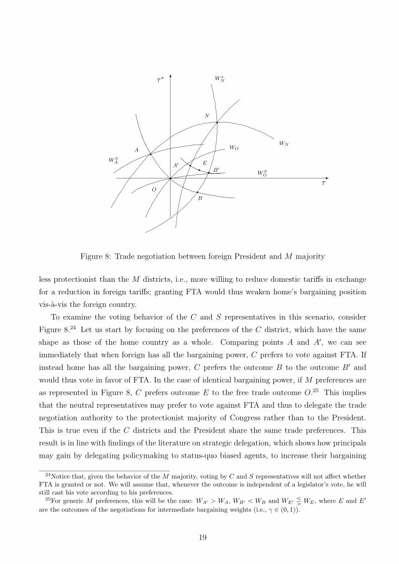
Figure 8: Trade negotiation between foreign President and M majority

less protectionist than the M districts, i.e., more willing to reduce domestic tariffs in exchange

for a reduction in foreign tariffs; granting FTA would thus weaken home’s bargaining position

vis-a-vis the foreign country.

To examine the voting behavior of the C and S representatives in this scenario, consider

Figure 8.24 Let us start by focusing on the preferences of the C district, which have the same

shape as those of the home country as a whole. Comparing points A and A′, we can see

immediately that when foreign has all the bargaining power, C prefers to vote against FTA. If

instead home has all the bargaining power, C prefers the outcome B to the outcome B′ and

would thus vote in favor of FTA. In the case of identical bargaining power, if M preferences are

as represented in Figure 8, C prefers outcome E to the free trade outcome O.25 This implies

that the neutral representatives may prefer to vote against FTA and thus to delegate the trade

negotiation authority to the protectionist majority of Congress rather than to the President.

This is true even if the C districts and the President share the same trade preferences. This

result is in line with findings of the literature on strategic delegation, which shows how principals

may gain by delegating policymaking to status-quo biased agents, to increase their bargaining

24Notice that, given the behavior of the M majority, voting by C and S representatives will not affect whetherFTA is granted or not. We will assume that, whenever the outcome is independent of a legislator’s vote, he willstill cast his vote according to his preferences.

25For generic M preferences, this will be the case: WA′ > WA, WB′ < WB and WE′ ⋚ WE , where E and E′

are the outcomes of the negotiations for intermediate bargaining weights (i.e., γ ∈ (0, 1)).

19

power in negotiations with other parties (e.g. Schelling, 1956; Jones, 1989; Segendorf, 1998).

Turning now to the S representatives, in the case illustrated in Figure 8, they will also prefer

A′ to A and B to B′. Hence, the more export-oriented S districts may also in some cases prefer to

vote against FTA, strategically delegating trade negotiation authority to a protectionist majority

in Congress. However, the likelihood of this happening is lower than for the C districts, since

the trade preferences of the S export districts differ more from those of the M import districts,

thus making delegation more costly. For example, in the case of identical bargaining power, if

M preferences are as represented in Figure 8, S representatives prefer outcome O to outcome

E.26

4.3.2 Majority of S Districts

Next, consider a scenario in which the representatives of the S export districts are the majority

in Congress (i.e., βS > 1

2). To analyze this case, we will use Figure 9 above. Again, the set of

feasible agreements that can be reached under FTA is represented by the AB segment of the CC

curve. Feasible agreements that can be reached in the absence of FTA, when Congress majority

negotiates directly with the foreign executive, are instead identified by the segment A′B′ of the

C ′C ′ curve. Point V represents the trade agreement that is efficient from the point of view of

the S majority and the foreign executive and gives the same level of utility to the home country

than the status quo. Notice that the President’s veto power in the last stage of the game rules

out agreements lying between V and A′.

In contrast to the case of a majority of M districts discussed above, in this scenario, the set

of feasible agreements between the Congress majority and the foreign executive is larger than

the corresponding set for the two executives. Moreover, the C ′C ′ curve now lies below the CC

curve. Notice that, like in the M majority case, in the absence of FTA, free trade is not a

possible negotiation outcome.

We can show that in this scenario M and C representatives will always vote in favor of FTA.

This is because, when negotiating with foreign, they will always prefer to be represented by the

President than by the S majority, since the executive is less eager to reach an agreement and

is thus able to achieve a more favorable deal. It can be easily shown that, for any given γ, an

outcome on the AB curve is always preferred to the corresponding outcome on the A′B′ curve.27

This establishes that it cannot be beneficial for a home legislator to delegate trade negotiation

authority to an agent who is keener than himself to reach an agreement with the foreign country.

26For generic M preferences, the following holds: WSA′ ⋚ WS

A , WB′ < WB and WSE′ ⋚ WS

E , where E and E′

are the outcomes of the negotiations for γ ∈ (0, 1).27Only in the limit case in which γ = 0, C districts would be indifferent between granting FTA or not. In this

case, because of the President’s veto power, both negotiation procedures would yield a level of utility WN for theC districts.

20

6

-

τ ∗

τ

WN

W ∗

N

NC

A

B

O

C

C′

C′

A′

B′

V

Figure 9: Trade negotiation between foreign President and S majority

Next, we turn to the voting behavior of S representatives. In line with our previous discussion

about strategic delegation, we can show that, although these representatives have a majority in

Congress, they might still prefer to vote in favor of FTA and delegate trade negotiation authority

to the executive.28

4.3.3 Majority of C Districts

Consider now the scenario in which the majority of Congress is made up of representatives of

the neutral C districts (i.e., βC > 1

2). Since the preferences of these districts coincide with

those of the entire country and thus of the President, negotiations between the majority of home

Congress and the foreign executive can be described using Figure 3 above. This implies that

fast track procedures will not affect the outcome of the negotiations.

In this case, there would be no reason to grant fast track authority to prevent amendments of

trade agreements by the majority of Congress. However, if legislators are impatient, they might

still prefer to vote in favor of FTA, so as to speed up the implementation of trade agreements (see

our discussion in Section 2 concerning the mandatory deadlines and limitations on congressional

28This is the case when the two countries have similar bargaining strength. Note that in the extreme case inwhich foreign has all the bargaining power (γ = 0), S representatives would be in favor of FTA if the Presidenthad no veto power (WS

A′ < WSA ) but are against FTA when the President has veto power (WS

V > WSA ). In the

opposite extreme (γ = 1), S representatives always oppose FTA (WSB′ > WS

B). For intermediate values of γ, wehave WS

E ⋚ WSE′ , where E and E′ are the negotiation outcomes achieved with or without FTA.

21

debate imposed by fast track procedures). We should thus expect C and S representatives to

always vote in favor of FTA, while M representatives may vote in favor or against it. To verify

this, notice from Figure 3 that any outcome on the AB segment of the CC contract curve is

always weakly (strongly) preferred by the C (S) district representatives to the status quo N .29

Representatives of the M districts, on the other hand, may or may not be better off in a trade

agreement compared to the status quo of Nash tariffs.

4.3.4 No Majority

Finally, let us examine the scenario in which none of the district types enjoys a majority in

Congress, i.e., βi < 1

2for all i ∈ M,S,C. This implies that in the absence of FTA, amendments

in stage 3 of the game can only be passed by a coalition of district representatives.

We assume that if a coalition is formed between two groups in Congress, its preferences are

given by a weighted sum of the preferences of their members, where the weights are given by the

districts’ share in Congress.

In line with our analysis of the previous scenario, we can show that it will never be in the

interest of the C or M congressmen to form a coalition with the S representatives. The intuition

behind this result is that, relative to a scenario in which trade negotiation authority is delegated

to the President, forming this coalition would always weaken home’s bargaining position vis-a-vis

the foreign country. Given this, the only possible coalition in the amendment phase is between

the C and M districts. While for the M representatives being in such coalition will always

be preferable than supporting FTA, the same is not always true for C. Below we show that

the voting behavior of the C representative depends crucially on how protectionist the resulting

coalition would be.

The trade preferences of the coalition of C and M districts are captured by

WC,M = βCWC + βMWM . (13)

Negotiations between the coalition and the foreign executive in case of no FTA can be captured

by Figure 7 above, where now WMN should be interpreted as representing WC,M

N . Notice that, the

steeper is WC,MN , the more likely it is that the C districts will vote for FTA rather than joining

the coalition. The intuition is that when the coalition becomes too protectionist, delegation to

a more status-quo biased agent becomes too costly.

Notice that the degree of protectionism of the coalition of C and M districts is captured by

29As discussed above, these congressmen may actually prefer to be represented in the negotiations by a moreprotectionist majority. However, this is not an option when βC > 1

2.

22

the slope of WC,M , which is given by

(dτ ∗

dτ

)C,M

= −

[(βMαM

1+ βCh)∂R1

∂τ+ (βM + βC)h

(∂T∂τ

+ ∂Ω

∂τ

)]

[(βMαM

2+ βCh)∂R2

∂τ∗+ (βM + βC)h ∂Ω

∂τ∗

] . (14)

Comparing (14) with equations (20) and (25) in the Appendix, we can easily show that the

coalition’s indifference curves are flatter than the indifference curves of the M representatives,

but steeper than those of the C representatives. It is also straightforward to verify that an

increase in βC will make the indifference curves of the coalition flatter; in turn, this will make

C representatives more likely to vote against FTA.

As far as S representatives are concerned, they will tend to vote in favor of FTA, preferring

the negotiation outcomes that would emerge when home is represented by the President to those

that would arise when home is represented by the coalition of C and M districts. However,

if this coalition is not too protectionist, the opposite might be true, particularly if the foreign

country enjoys a larger bargaining power (i.e., γ → 1). This is in line with our discussion of the

voting behavior of S representatives in the case of M majority.

4.4 FTA Voting Decisions and International Trade Agreements

In what follows, we summarize our discussion in Section ?? in five main results. The first two

propositions concern the impact of fast track procedures on the outcome of trade negotiations

between home and foreign.

Proposition 1 Unless βC > 1

2, free trade can only be achieved under FTA.

To verify this, notice that under fast track authority, when negotiations take place between

the home and foreign executives, the set of efficient trade agreements is identified by the CC

contract curve in Figure 3 above, which goes through the free trade point 0. In the absence of

FTA, the contract curve will be either above the CC curve (C ′C ′ in Figure 7) or below (C ′C ′ in

Figure 9), depending on the type of Congress composition, and will thus not pass through point

0.30

Proposition 2 Unless βS > 1

2, foreign prefers to negotiate with home under FTA.

In the absence of FTA, it is as if the foreign executive negotiates directly with the majority

in the home Congress. Except for the case in which the export-oriented S representatives hold

30As discussed above, in the absence of FTA, free trade can only be achieved if C representatives hold amajority of seats in Congress. In this case, the contract curve identifying efficient agreements between the foreignexecutive and the majority of home Congress would coincide with the CC curve in Figure 3.

23

a majority of seats in Congress (βS > 1

2), this leads to worse negotiation outcomes from the

point of view of the foreign country than those that could be achieved under FTA. The intuition

behind this result is that lack of FTA strengthens home’s bargaining positions in the negotiations

with foreign.31 This result can explain why foreign countries are often reluctant to negotiate

trade agreements with the United States in the absence of FTA.32

The remaining three results relate to the FTA voting behavior of home’s congressmen.

Proposition 3 Home legislators will never delegate trade negotiating authority to the agent that

is keener to reach an agreement with the foreign country.

When voting for or against fast track procedures, home legislators must implicitly decide

who should represent the country in the negotiations with foreign. The choice is either between

oneself and the President (in the case of legislators who control the majority in Congress); or

between a majority in Congress and the President (in the case of legislators who do not hold a

majority). Our analysis above shows that, when taking this decision, legislators will never choose

the agent who has the weaker bargaining position vis-a-vis the foreign country. For example,

the M representatives will vote against FTA if they hold a majority in Congress—since in this

case the President is the weaker country representative—but will vote in favor of FTA if the S

districts hold a majority—since in this case the President is the tougher bargainer. Similarly, C

representatives might decide to vote against FTA if the majority of Congress is more protectionist

than the President, but would always vote in favor of FTA otherwise.

In our discussion of the four possible scenarios of Congress composition, we established that,

except for the case in which S districts are a majority in Congress, M representatives will never

vote in favor of FTA, S representatives will be unlikely to vote against, while C representatives

might vote in favor or against. The likelihood that legislator i will vote in favor of FTA should

thus increase in the extent to which his constituency is relatively specialized in the production

of the export good, as captured by the ratioαi

2

αi1

. This implies the following:

Proposition 4 Unless βS > 1

2, the likelihood that a home legislator votes in favor of FTA

increases with the degree to which his district is export-oriented compared to the country as a

whole.

31Notice that this is true for scenarios in which M districts hold a majority of seats in Congress and for scenariosin which none of the district types enjoys a majority in Congress. For the case of C majority, FTA should notaffect negotiation outcomes; however, foreign should still prefer to negotiate under FTA on the ground that itallows a faster implementation of trade agreements.

32For example, during the negotiations of the Uruguay Round, U.S. trade officials were subject to strongpressures from other GATT members to come to the negotiating table with fast track authority. Similarly,Proposition 2 can explain why Chile only negotiated a free trade agreement with the U.S. in 2003, after the latestrenewal of FTA, rather than during the period between 1994 and 2002, when fast track authority lapsed.

24

Our analysis in Section 4.3.4 also suggests that, if none of the district types has the majority

in Congress, the neutral C districts will only vote against FTA in stage 2 of the game if they can

reach more favorable negotiation outcomes by forming a coalition with the M representatives

in stage 4 of the game; in turn, this can only happen if such coalition is not too protectionist,

which is more likely to be the case the larger is βC (or the smaller is βM). We can thus state

the following result:

Proposition 5 If βi < 1

2for all i ∈ M,S,C, the likelihood of C representatives voting in

favor of FTA decreases with βC.

4.5 Empirical Predictions

In the empirical analysis that follows we will test the last two theoretical results concerning

FTA voting behavior (Propositions 4 and 5 above), which we can restate in terms of empirical

predictions:

• The likelihood of a U.S. congressman voting in favor of FTA should increase with the

degree to which his district is relatively export-oriented compared to the U.S. as a whole;

• When no group of district representatives has the majority in Congress, M representatives

will vote against FTA, while S representatives will tend to vote in favor; furthermore, the

likelihood of C representatives voting in favor of FTA should decrease with their relative

share in Congress.

Before describing the details of our empirical investigation, a few remarks are in order concerning

the link between our theoretical analysis and its empirical counterpart. In Sections 4.3 and 4.4,

we have examined legislators’ voting behavior in all possible scenarios in terms of Congress

composition: 1) majority of M districts; 2) majority of S districts; 3) majority of C districts;

and 4) no majority. As shown in the next section, our dataset does not include situations in

which M or S districts have a majority in the U.S. Congress; therefore only scenarios 3) and 4)

are empirically relevant. However, this does not pose a problem for our empirical analysis, since

the predictions of our two main propositions are valid in the scenarios that we do observe.

Consider first Proposition 4, which characterizes voting behavior in scenarios 1), 3) and 4) and

predicts that the likelihood that a U.S. legislator votes in favor of FTA should increase with the

degree to which his constituency is export-oriented compared to the country as a whole. Since

scenario 2) is not empirically relevant, we can directly assess the validity of this proposition.

Consider next Proposition 5, which predicts that in the case of no majority C legislators should

be more likely to vote in favor of fast track authority the larger is their share in Congress. Notice

25

that in the remaining scenarios the voting behavior of C representatives should not be affected

by their share. Evidence of a negative relationship between C’s share and their likelihood to

vote in favor of FTA would thus provide empirical support for this proposition.

Notice that we are unlikely to observe votes on fast track when the majority of Congress is

against granting it. Indeed, as it can be seen from Table 1, with the exception of House Resolution

2621 of September 25, 1998 all votes ended up with Congress granting FTA.33 Interestingly, this

might explain why scenario 1 is not included in our dataset, since it would always result in fast

track not being granted. However, this issue does not pose a problem for our empirical analysis,

which concerns FTA voting behavior of individual U.S. congressmen, rather than the outcomes

of FTA decisions.

5 Data

In the empirical analysis presented below, we will examine the determinants of FTA voting

decisions by U.S. congressmen. The objective of our analysis is to verify whether the legislators’

voting behavior reflects the trade policy interests of their constituencies, as predicted by our

theoretical model. To do so, we will try to isolate congressmen’s trade policy interests from

other factors which might affect their FTA voting decisions, such as their ideological preferences

or which chamber of Congress they belong to.

Table 1 in Section 2 above provides details of all the votes granting or extending FTA that

occurred in Congress, from the first one in 1973 till the last one in 2002.34

Differently from the theoretical analysis where we used the words constituency and district

interchangeably, empirically we have to distinguish the 435 congressional districts that elect one

member each for the House of Representatives and the 50 states that elect two representatives

each for the Senate. As it can be seen from Table 1 though, for each decision in the House and

Senate less than 435 and 100 votes, are respectively reported. This is because some congressmen

may not be present or may decide to abstain. Moreover, a seat in Congress may be vacant at

any point in time because of special circumstances (e.g. resignation, death).

Overall, thirteen votes on FTA have been held in Congress including the House and Senate

resolutions of disapproval that were rejected in 1991.35 Seven of them took place in the House,

33In some situations, the President may decide not to request a vote on FTA, anticipating that the outcomewill be negative. For example, this is what happened in November 1997, when President Clinton agreed to holdoff on the floor vote in the House, after House Speaker Gingrich had reportedly said that the vote was 5-25 votesshort of passage (see Shoch, 2002).

34When multiple votes occurred for each decision, only the final vote (i.e., Conference Report) is reported.35As a result of these resolutions, FTA was extended for trade agreements signed between May 31, 1991 and

May 31, 1993. Compared to the other votes, the results in 1991 have the opposite interpretation (i.e., a vote infavor of disapproval is a vote against FTA).

26

Table 3: Definition of variables and sourcesVariable Definition Source

V oteit Vote cast by congressman i in year t Up to 1996: ICPSR Study number 4

Dummy variable equal to 1 if ‘yea’ and 0 if ‘nay’ From 1997: http://www.voteview.com

λit Employees in year t of district i in export industries divided by County Business Patterns

employees of district i in import industries

λUSt U.S. employees in year t in export industries divided by As for λi

t

U.S. employees in import industries

Λit Ratio λi

t/λUSt As for λi

t

Democrat Dummy variable equal to 1 if a congressman is a Democrat As for Vote

Conservative rating Rating (0–100) of Congressmen by American Conservative Union As for Vote

Senate Dummy equal to 1 for Senators http://www.acuratings.org/

Party as President Dummy equal 1 if Congressman and president belong to same party As for vote

S, M , C districts Dummy equal to 1 if district is of type S, M , or C As for λit

Congressional Districts Aggregate of counties included in each district 1973-1982: ICSPR dataset 8258;

1983-2012: provided by Christopher Magee

Import/export industries Industries in which the U.S. is a net importer/exporter Feenstra (1996, 1997), Feenstra et al. (2002),

(annual basis) and U.S. ITC, IMF BoP Statistics

27

and six in the Senate36

For each vote, the identity of congressmen, their party affiliation, their state or district and

their vote (in favor or against FTA) has been collected from roll call voting records. Table 3

provides details on the definitions and sources for all the variables used in our regressions (or

used in the construction of the regressors).

Following our theoretical model, the main determinant of a congressman’s vote refers to

his constituency’s trade position with respect to the United States at large. This requires the

construction of district-specific and time-varying variables. Such variables are relatively easy to

construct for the Senate, since each State always elects two Senators in state-wide elections. The

case of House representatives is more complicated, since ready-made series are not available for

the variables of interest. In particular, we encountered two main problems to obtain our proxy

for a district’s trade preferences.

The first problem is that district-specific information for the House must be obtained by

aggregating county-level data, for which industry level information can be obtained from the

County Business Patterns (CBP) series. To complicate matters further, a county may be split

and various bits assigned to different districts.37 Second, the geographic definition of Con-

gressional Districts changes every ten years following the Decennial Census (as a result of the

so-called “redistricting”). The 435 districts are assigned across the United States depending on

population, with each State having at least one district. Given that our sample spans thirty

years (i.e., 1973-2002), we need to track changes over three censuses.38

To deal with the first issue, county and state level data have been extracted from the CBP.

This is an annual series of reports by the Bureau of the Census providing detailed information on

U.S. business and industries. The CBP report annual data on employment by SIC manufacturing

industries up to 1997 and by NAICS manufacturing industries from 1998.39

Notice that employment data in the CBP are withheld when their disclosure would allow

researchers to identify firms. In such cases, a flag gives the interval where the actual data

36The Senate did not vote on the extension in 1998 since the House had already rejected it.37For example, in the 1990’s, Los Angeles county (California) was split among 17 congressional districts and

Cook county (Illinois) was split among 12 congressional districts.38For example, Alaska has always had only one Congressional District; between the first FTA vote in 1974 and

the last one in 2002, California went from 43 to 52 districts, while New York went from 39 to 31. Minor changesmay occur between two consecutive censuses because of court actions; the regression results reported in Section6 ignore these changes.

39The CBP series mostly contains data on employment in manufacturing industries, with very little detailedinformation for the agricultural sector. However, manufacturing industries represent the lion’s share of totalimports and exports of the United States (i.e., at least 70 percent in each year from 1970 until today). Moreover,many agriculture-related activities are classified as manufacturing and are thus included in our dataset (e.g.,dairy products, grain mill products, and sugar are included in SIC 20 and NAICS 311). In Section 7, where wereport the results of various robustness checks, we will include information on agriculture employment, as wellas on employment in the service sector.

28

belongs to.40 These flags have been used to input values (i.e., the mid point of each interval)

for the missing observations. In order to minimize the problem of undisclosed data, we use CBP

employment data at the 2-digit SIC and 3-digit NAICS levels rather than at more disaggregated

levels. Unfortunately, the CBP do not provide any flag for the data withheld in 1973. Treating

these observations as missing results in a substantial underestimate of the employment in each

county and, consequently, congressional district, which is why we have decided to omit the House

vote of 1973 from our main estimations. Thus, we are left with 3, 068 observations (i.e., all the

votes from 1974 until 2002 as reported in Table 1).

Tables 9 and 10 in the Appendix report the list of manufacturing industries included in our

analysis. For each year, each industry has been classified as being import-competing (export),

if the U.S. as a whole was a net importer (exporter) for that industry in that year. For each

county, we computed the number of employees in import (export) oriented sectors. Then, we

constructed the corresponding figures for each Congressional district, by aggregating data for

the counties included in that district. For those counties split across more than one district, we

followed Baldwin and Magee (2000a,b), among others, imputing employees proportionally to the

share of population of a county assigned to that district.41 Similar procedures to define import

and export-oriented industries have been applied to state data to obtain analogous series for the

Senate.

Having constructed the series of employees in import and export industries in each con-

stituency (congressional district or state), we can then construct the main regressors of interest

for our analysis. For each constituency i at time t, we define the ratio of employees in export

industries (indexed by x) to import-competing industries (indexed by m), as well as this ratio

relative to the United States as a whole (indexed by US):

λit =

∑

x

Lix,t

∑

m

Lim,t

, (15)

λUSt =

∑

x

LUSx,t

∑

m

LUSm,t

, (16)

40For example, between 0 and 19 employees, between 20 and 99 employees and so on.41We are grateful to Christopher Magee who provided us with the files for mapping counties into districts

from 1983 until 2002, and to James Snyder who pointed out where to find a similar information for the period1973-1982.

29

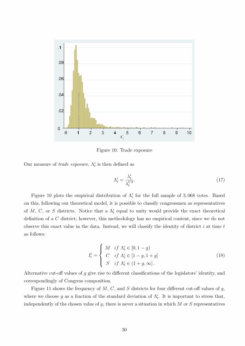
Figure 10: Trade exposure

Our measure of trade exposure, Λit is then defined as

Λit =

λit

λUSt

. (17)

Figure 10 plots the empirical distribution of Λti for the full sample of 3, 068 votes. Based

on this, following our theoretical model, it is possible to classify congressmen as representatives

of M , C, or S districts. Notice that a Λit equal to unity would provide the exact theoretical

definition of a C district; however, this methodology has no empirical content, since we do not

observe this exact value in the data. Instead, we will classify the identity of district i at time t

as follows:

I it =

M if Λit ∈ [0, 1 − g)

C if Λit ∈ [1 − g, 1 + g]

S if Λit ∈ (1 + g,∞] .

(18)

Alternative cut-off values of g give rise to different classifications of the legislators’ identity, and

correspondingly of Congress composition.

Figure 11 shows the frequency of M , C, and S districts for four different cut-off values of g,

where we choose g as a fraction of the standard deviation of Λit. It is important to stress that,

independently of the chosen value of g, there is never a situation in which M or S representatives

30

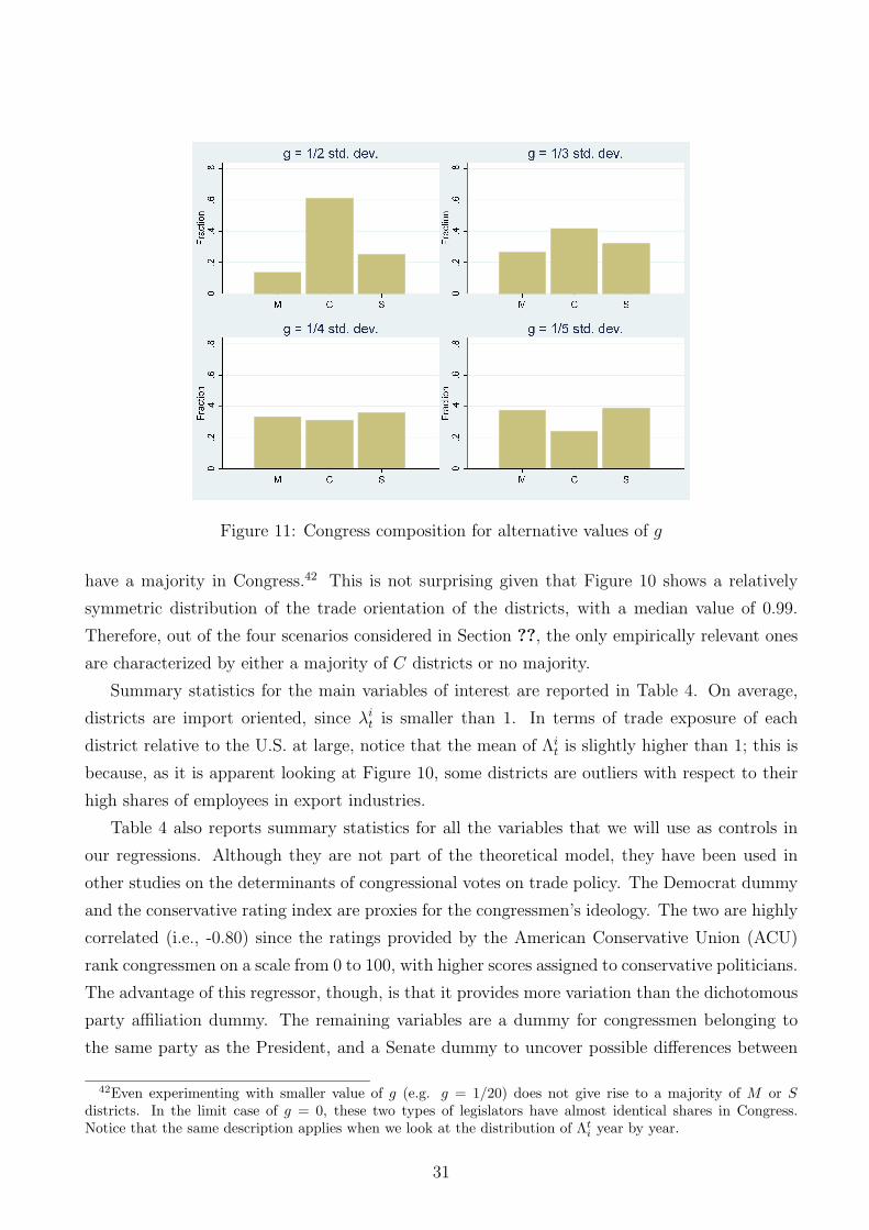
Figure 11: Congress composition for alternative values of g

have a majority in Congress.42 This is not surprising given that Figure 10 shows a relatively

symmetric distribution of the trade orientation of the districts, with a median value of 0.99.

Therefore, out of the four scenarios considered in Section ??, the only empirically relevant ones

are characterized by either a majority of C districts or no majority.

Summary statistics for the main variables of interest are reported in Table 4. On average,

districts are import oriented, since λit is smaller than 1. In terms of trade exposure of each

district relative to the U.S. at large, notice that the mean of Λit is slightly higher than 1; this is

because, as it is apparent looking at Figure 10, some districts are outliers with respect to their

high shares of employees in export industries.

Table 4 also reports summary statistics for all the variables that we will use as controls in

our regressions. Although they are not part of the theoretical model, they have been used in

other studies on the determinants of congressional votes on trade policy. The Democrat dummy

and the conservative rating index are proxies for the congressmen’s ideology. The two are highly

correlated (i.e., -0.80) since the ratings provided by the American Conservative Union (ACU)

rank congressmen on a scale from 0 to 100, with higher scores assigned to conservative politicians.

The advantage of this regressor, though, is that it provides more variation than the dichotomous

party affiliation dummy. The remaining variables are a dummy for congressmen belonging to

the same party as the President, and a Senate dummy to uncover possible differences between

42Even experimenting with smaller value of g (e.g. g = 1/20) does not give rise to a majority of M or Sdistricts. In the limit case of g = 0, these two types of legislators have almost identical shares in Congress.Notice that the same description applies when we look at the distribution of Λt

i year by year.

31

Table 4: Summary statistics

Variable Observations Mean Std. dev.

V oteit 3,068 0.697 0.460

λit 3,068 0.693 0.684

Trade exposure 3,068 1.194 0.829

Democrat 3,068 0.559 0.497

Conservative rating 3,065 46.704 37.447

Senate 3,068 0.207 0.405

Party as President 3,068 0.495 0.500

the two chambers of Congress.

6 Empirical Methodology and Results

The dependent variable in our empirical analysis, V oteit is dichotomous and equals one if the

congressman has voted in favor of granting or extending FTA and zero otherwise. Our baseline

specification is thus given by

Prob(voteit = 1) = Φ

(α + β1X

it + β2Z

)(19)

where Φ (·) is the cumulative normal distribution (i.e., probit model). Xit is a matrix of district-

specific variables (i.e., all the variables listed in Table 4), Z is a matrix of additional controls,

which may or may not be time-invariant and district specific (e.g., time or state fixed effects) and

α, β1, and β2 are the vectors of parameters to be estimated. Depending on the specification, the

main variable of interest (i.e., the district’s trade exposure) may be continuous (Λit) or captured

by the dummy variables defined in (18), with possibly different cut-off values for g. In order to

facilitate the interpretation of the estimated coefficients, in the tables we report marginal effects

(calculated at the mean of each regressor).

Moving to the results, we first want to assess the validity of the voting prediction contained

in Proposition 4, according to which the likelihood that a legislator will vote in favor of FTA

should increase with the degree to which his constituency is relatively export-oriented compared

to the U.S. as a whole. To capture the trade policy preferences of the legislators’ constituencies

we employ the continuous variable Λit. The results for this specification are presented in Table

5 below.

In column (1), the simplest possible specification is reported, where the only explanatory

variables are Λit and a set of year effects.43 The prediction of the theoretical model is clearly

43The estimates of various fixed effects are not reported to save on space. All the results and tests not reportedin the text are available upon requests.

32

confirmed in the data, as the estimated coefficient of Λit is positive and significant at 1 percent

level. In other words, a congressman is more likely to vote in favor of granting or extending

FTA the more export oriented his district is compared to the whole of the U.S. The set of year

dummies is jointly significant and their coefficients indicate a decreasing likelihood over time of

voting in favor of FTA.44 This suggests an erosion of the American consensus in favor of trade

liberalization.

The remaining columns of Table 5 provide variations on the first regression. In the second

specification, state effects are included (and they are jointly significant), without any qualitative

change in the results. Clearly, this set of dummies controls for state-wide time-invariant deter-

minants and it results in an increased fit of the model.45 Still, the qualitative result on Λit is

unchanged although the point estimate of its marginal effect is higher. Keeping the state effects

and adding a Senate dummy variable in column (3) has no effect on the main variable of interest.

However, Senators are in general more likely to vote in favor of FTA (6 percent on average).

As an additional control, in column (4) we include a dummy variable that takes a value of one

if the congressman belongs to the Democratic party, and zero otherwise. Also in this case, the

added regressor is significant and negative but the other coefficients are left unchanged. As an

alternative, in column (5) we use the conservative rating from the ACU.46 It is highly significant

and positive, indicating that more conservative congressmen are more likely to vote in favor of

FTA.47 Both results suggest that the Republicans are more liberal on trade, a claim that may

seem odd since Democrats have long been perceived as the traditional champions of free trade.

However, their position has changed over time (see Hiscox, 1999). Indeed, around 1970 the

parties realigned their trade policy stances as a result of more protectionist unions supporting

the Democrats, while Republicans gained ground among export-oriented businesses (see Destler,

1980). For example, in Karol (2000)’s analysis of various trade votes in the 1950s and 1990s,

the Democrat dummy variable is consistently positive and significant in the 1950s, but becomes

negative and significant for the votes in the 1990s.

The results are also very similar if we check for whether the congressman and the President

are aligned, i.e. they belong to the same party. As it turns out, the probability of a congressman

voting in favor of FTA increases if the congressman belongs to the same party as the President.

44Such trend may be due to various factors, including a strong increase in trade volumes, which might havelead to larger adjustment costs associated with trade liberalization, and the concerns over non-trade issues suchas labor and environmental standards (see Elliot, 2000). Notice that Λi

t would also be significant at 1 percentand with an almost identical marginal effect if the year dummies were not included, although the Pseudo R2

would be lower.45The inclusion of state effects forces us to drop the 17 observations for congressmen from Wyoming since they

all and always voted in favor of FTA.46These two variables can not be included simultaneously since they are highly correlated, i.e., -0.80.47Since such ratings are not available for three congressmen and the fit of the model is slightly lower, in the

following, we will use the Democrat dummy.

33

Table 5: Empirical results with continuous variable: marginal effects

Regressor (1) (2) (3) (4) (5) (6) (7) (8)

Trade exposure 0.032*** 0.059*** 0.059*** 0.053*** 0.057*** 0.053*** 0.055*** 0.075***

(0.011) (0.013) (0.013) (0.013) (0.013) (0.013) (0.016) (0.026)

Senate 0.063*** 0.073*** 0.073*** 0.073***

(0.023) (0.024) (0.024) (0.024)

Democrat -0.286*** -0.288*** -0.328*** -0.148***

(0.015) (0.015) (0.017) (0.039)

Conservative rating 0.004***

(0.0002)

Party as President -0.013

(0.019)

Year effects included included included included included included included included

State effects included included included included included included included

Observations 3,068 3,051 3,051 3,051 3,048 3,051 2,506 476

Log likelihood -1,550.18 -1,442.63 -1,419.35 -1,269.48 -1,294.37 -1,269.24 -1,049.34 -174.50

Pseudo R2 0.18 0.24 0.24 0.32 0.31 0.32 0.34 0.31

χ2 478.35*** 570.05*** 566.90*** 546.11*** 541.67*** 540.46*** 454.25*** 147.63***

Predicted Prob. 0.75 0.77 0.77 0.78 0.78 0.78 0.76 0.86

Notes: Dependent variable: voteit = 1 if a Congressman votes in favor of FTA, votei

t = 0 otherwise. Robust standard

errors in parenthesis; *** denotes significance at 1% level; ** 5% level; * 10% level. Marginal effects for dummy

variables calculated as discrete changes from 0 to 1.

34

This is consistent with the fact that Republicans are more likely to vote in favor of FTA and

most FTA votes occurred under a Republican President.48 However, only the Democrat dummy

is significant (and still negative) if both dummy variables are included at the same time (column

6). In other words, the alignment between the President and Congress does not seem to matter

once we control for the congressmen’s party affiliation.49

Finally, in the last two columns of Table 5 we separately consider the behavior of members of

the House and the Senate. These specifications are more flexible than simply including a Senate

dummy, since all the coefficients, and not only the constant, are allowed to take different values

between the two chambers.50 The marginal effects of trade exposure and the Democrat dummy

for the Senate show different magnitudes, and are always significant. In particular, senators

are more sensitive to the trade exposure of their constituency and Democrat senators are more

liberal than House Democrats.

We then turn to evaluate the predictions of Proposition 5, according to which, when no group

of district representatives has the majority in Congress, M representatives should vote against

FTA, while S representatives will tend to vote in favor; furthermore, the likelihood of C repre-

sentatives voting in favor of FTA should decrease with their relative share in Congress. Instead

of using a continuous variable, the specifications reported in Table 6 use the classifications of

constituencies into M , C or S types as defined in equation (18). Taking the C constituencies

as the base (omitted) category, the two specifications with different cut-off values of g show

that congressmen from S and M constituencies always exhibit a statistically different voting

behavior on FTA bills. In line with our theoretical model, representatives from S constituencies

are always more likely to vote in favor of granting or extending FTA than representatives from

M constituencies. This result holds across the different cut-off values chosen for g. However,

consistently with Proposition 5, the choice of g bears an effect on the voting behavior of con-

gressmen from C constituencies: if g = 1/4, C district representatives represent a smaller share

of Congress and are thus more likely to favor FTA. As a result, their voting behavior is not

statistically different from that of S representatives. When instead g = 1/3, C representatives

are a larger share of Congress and are thus less likely to support FTA, and their voting behavior

is significantly different from that of M and S legislators. As for the estimates for the Senate

48Only three rounds of the votes listed in Table 1 occurred under a Democrat President (i.e., the TradeAgreement of Act of 1979 under President Carter; the extension of FTA in 1993 for completing the UruguayRound and the failed extension in 1998 under President Clinton).

49We have also considered including a dummy variable for votes that occurred during the second term of aPresident. Unfortunately, this dummy is collinear with the set of year fixed effects, since it does not present anywithin-year variation: the only votes which took place during a second presidential mandate were the Senate andHouse votes in 1988 (Reagan administration) and the House vote in 1998 (Clinton administration).

50Some more observations are lost because of no variation in the dependent variable within the House and/orthe Senate for some States.

35

and Democrat dummies, they are identical to their counterpart in Table 5.

Table 6: Using dummy variables: marginal effects

g = 1

3std. dev. g = 1

4std. dev.

Regressor (1) (2)

S constituency 0.046** 0.025

(0.020) (0.021)

M constituency -0.047** -0.046**

(0.022) (0.022)

Senate 0.070*** 0.068***

(0.024) (0.024)

Democrat -0.288*** -0.287***

(0.015) (0.015)

Year effects included included

State effects included included

Observations 3,051 3,051

Log likelihood -1,270.38 -1,272.53

Pseudo R2 0.32 0.32

χ2 551.83*** 552.49***

Predicted Prob. 0.78 0.78

Notes: Dependent variable: voteit = 1 if a Congressman

votes in favor of FTA, voteit = 0otherwise. Robust stan-

dard errors in parenthesis; *** denotes significance at 1%

level; ** 5% level; * 10% level. Marginal effects for dummy

variables calculated as discrete changes from 0 to 1.

Finally, we focus on the behavior of congressmen from C constituencies to assess more directly

the empirical validity of Proposition 5. Since Proposition 5 refers to scenarios in which no group

of constituencies has a majority in Congress, we focus on the cut-off values of g = 1

4in Figure

11, for which C constituencies never have a majority.51 Notice that year fixed effects are not

included in these specifications, since they are perfectly collinear with the two main regressors

of interest. The results reported in Tables 5 and 6 above show that, when the year fixed effects

are included, voting in favor of FTA becomes less likely over time (i.e., the year fixed effects

are significant, negative and with bigger absolute values for recent years). To make sure that

51Notice that, although Figure 11 shows that for g = 1

3on average C constituencies do not hold a majority,

their share is higher than 0.50 in some years. For this reason, we focus here on the case of g = 1

4.

36

our regressors βC and βC/(βC + βM) do not simply pick up some of these time effects, we have

included a linear trend in the regressions. Consistently with a decreasing likelihood of FTA over

time, the estimated coefficient for this trend is significant at 1% and negative.

Table 7 contains six different specifications where only the votes of representatives from C

constituencies are included as the dependent variable. In the first three columns, the main

regressor of interest is the share of C constituencies, i.e., βC . In the remaining three columns,

instead, the share of C constituencies in the coalition of C and M constituencies is included,

i.e., βC/(βC + βM). Focusing on the first two rows of Table 9, we see that the empirical results

are consistent with Proposition 5, since C congressmen are more likely to vote against FTA

the higher their share in Congress or in their coalition with the M representatives. The point

estimates in the last three columns are lower since βC/(βC + βM) is always higher than βC and

the two variables are highly correlated (i.e., 0.90).52

As for the effect of the additional controls, their impact is comparable with the previous

specifications. Senators are more likely to vote in favor of FTA, while Democrat congressmen

are less favorable, also when ideology is measured with the continuous conservative rating. The

only noticeable difference with respect to Table 7 is that the dummy variable for the alignment

between congressmen and the President is now significant and positive when included along with

the Democrat dummy.53

As mentioned above, the results presented in Table 7 were based on a classification of legisla-

tors using g = 1/4 as a fraction of the standard deviation of our trade exposure measure, which

corresponds to a scenario in which there is no majority.

The fact that these results provide strong evidence for the specific voting behavior of C

representatives predicted by Proposition 5 for the case of no majority—a type of voting behavior

that would only arise in such a scenario—suggest that this was indeed the empirically relevant

one. This implies that if we were to use larger values of g we would artificially give rise to

scenarios in which C constituencies have a majority in Congress, hence misclassifying some of

the M and S legislators; in turn, this should lead to weaker evidence of a negative relationship

between the voting behavior of C constituencies and their share in Congress. Indeed, when we

tried running our regressions for higher values of g (e.g., 1/2 and 2/3), we found that this leads

to lower estimates of the coefficients in Table 9 (column 1), and that these estimates become

insignificant for large enough g.

52Notice that, if we exclude the variable Trend from the set of controls, the shares βC and βC/(βC + βM )remained negative and significant at 1%, although with much higher (in absolute values) point estimates.

53The inclusion of the state fixed effects results in the exclusion of 90 observations because of the lack ofvariations within some states over time. The results are similar if the state effects are not included.

37

Table 7: Empirical results for C constituencies: marginal effects

Regressor (1) (2) (3) (4) (5) (6)

βC -0.023*** -0.025*** -0.022***

(0.007) (0.007) (0.007)

βC/(βC+βM) -0.012*** -0.013*** -0.012***

(0.004) (0.004) (0.004)

Senate 0.126** 0.126** 0.124** 0.122*** 0.120*** 0.119**

(0.045) (0.045) (0.046) (0.045) (0.045) (0.046)

Democrat -0.352*** -0.343*** -0.347*** -0.339***

(0.031) (0.031) (0.030) (0.030)

Conservative rating 0.005*** 0.005***

(0.001) (0.000)

Party as President 0.075** 0.077**

(0.034) (0.033)

Trend -0.021*** -0.020*** -0.022*** -0.027*** -0.026*** -0.028***

(0.004) (0.004) (0.004) (0.003) (0.003) 0.003

State effects included included included included included included

Observations 849 848 849 849 848 849

Log likelihood -371.37 -374.11 -369.18 -371.78 -374.52 -369.44

Pseudo R2 0.31 0.31 0.32 0.32 0.31 0.32

χ2 213.04*** 209.10*** 209.83*** 205.21*** 199.22*** 201.70***

Predicted Prob. 0.73 0.73 0.73 0.74 0.73 0.74

Notes: Dependent variable: voteit = 1 if a Congressman votes in favor of FTA, votei

t = 0

otherwise. Only congressmen from C constituencies (defined with g = 1

4) are included.

Robust standard errors in parenthesis; *** denotes significance at 1% level; ** 5% level; *

10% level. Marginal effects for dummy variables calculated as discrete changes from 0 to 1.

7 Robustness Checks

In this section, we discuss the results of a series of estimations that we have performed to check

the robustness of our empirical results. All the specifications not explicitly reported are available

upon request.

The first three robustness checks are related to our measure of trade orientation. As men-

tioned above, the CBP series that we employ to construct our Λti variable mostly contains data

on employment in manufacturing industries, with very little detailed information about employ-

38

ment in agriculture. Although Λti includes employment in agriculture-related sectors such as

dairy products, to separately assess the role of agriculture in shaping individual congressman

behavior, we have tried to include as an additional control in all our regressions the share of

population employed in agriculture in each congressional district, which can be obtained from

the Census of Agriculture. In all cases, in line with previous results reported by Baldwin and

Magee (2000a,b), the estimated coefficient was negative but not significant, and there was no

qualitative or quantitative change for the other explanatory variables.

The definition of Λti that was used in our baseline regressions also excluded employment

in services, even if the CBP does include information on employment in some service sectors.

We have excluded services because there is no available data on trade in services by the same

SIC or NAICS codes used by the CBP, which prevents us from directly classifying the various

activities within services as being import or export oriented. Data on services can be derived

though from balance of payments statistics (BoP statistics) and are available in large groupings

(e.g., transportation, travel, construction). Moreover, a known problem with these data is its

reliability, since they are more difficult to collect than those on traded goods.

Bearing in mind these caveats, we have manually matched SIC and NAICS codes to the

categories of services available from the International Monetary Fund BoP statistics. Notice

though, that detailed service data by major categories are only available from 1986 (e.g., the

categories ‘Construction’ and ‘Computer and information services’ were not reported in earlier

years). Thus, when using service data we had to restrict our sample to the votes that occurred

from 1988 onward. Table 11 in the Appendix reports the correspondences that we created in

order to use CBP data on employment for service-related sectors. Unfortunately, we could not

match some service sectors to specific SIC or NAICS code.54 The included sectors account on

average for more than 70 percent of the value of services exports and imports for the years

included in our empirical analysis. Constructing our Λti including service data, we obtain a

distribution of this variable which is characterized by fewer extreme values (i.e., the maximum

value is 6.3 compared to 9.5 in Figure 10) and a smaller standard deviation (i.e., 0.74 versus

0.83). This may be the result of the fact that employment in services is less geographically

concentrated than in manufacturing.

54The excluded sectors are ‘Postal and courier services’, ‘Royalties and license fees’, ‘Insurance services’, ‘Finan-cial services’, ‘Personal, cultural, and recreational services’, and ‘Government services’. Insurance and financialservices had to be excluded since we cannot match them separately to SIC and NAICS categories and theirnet balances exhibit different signs (i.e., the United States is a net importer (exporter) of insurance (financial)services).

39

Table 8: Robustness check using services: marginal effects

Including Including

services services

Regressor (1) (2) (3) (4)

Trade exposure 0.086*** 0.071***

(0.019) (0.022)

βC -0.028*** -0.015**

(0.008) (0.006)

Senate 0.110*** 0.110*** 0.152** 0.152***

(0.031) (0.031) (0.055) (0.051)

Democrat -0.367*** -0.374*** -0.422*** -0.435***

(0.019) (0.019) (0.035) (0.036)

Trend -0.020*** -0.021***

(0.005) (0.005)

Year effects included included

State effects included included included included

Observations 2,484 2,484 724 757

Log likelihood -1,550.18 -1,193.51 -347.83 -367.03

Pseudo R2 0.27 0.27 0.28 0.27

χ2 493.67*** 488.05*** 566.90*** 183.92***

Predicted Prob. 0.68 0.68 0.65 0.67

Notes: Dependent variable: voteit = 1 if a Congressman votes in favor of FTA,

voteit = 0 otherwise. Data are from the period 1988-2002. Only congressmen

from C constituencies are included in columns (3) and (4) (defined with g = 1

4

and g = 1

3, respectively). Robust standard errors in parenthesis; *** denotes

significance at 1% level; ** 5% level; * 10% level. Marginal effects for dummy

variables calculated as discrete changes from 0 to 1.

The results of two of our main specifications when constructing our Λti variable with em-

ployment in service sectors are reported in Table 8. Columns (1) and (3) replicate the earlier

results with data only on manufacturing on the shorter sample period for which service data are

available (i.e., votes from 1988) in order to allow a direct comparison of the effect of including

employment on services. The reported marginal effects show that the qualitative results are un-

changed although the point estimates are somewhat larger than in the benchmark specifications

in Tables 5 and 7. When we also include service data, all the results continue to hold. In column

(2), the coefficient on trade exposure is positive and significant at 1 percent. The point estimate

40

for βC in specification (4) is also very similar to column (3) although the observations included

in the last two columns are not the same since the identity of C constituencies is influenced by

the inclusion of employment in service sectors. Thus, our results are robust to the inclusion of

services, even if there are various problems related to their use, not least that the sample period

is reduced.55

A final check concerning how we constructed our Λti variable concerns the issue of within-

county heterogeneity. Recall that we constructed employment variables for congressional districts

by aggregating county-level data. For those counties which are split across more than one district,

we imputed employees proportionally to the share of population of a county assigned to that

district. This procedure may lead to imprecise values of Λti for those counties which are split

in many districts, if they are very diverse in terms of the geographic distribution of production

activities. To deal with this issue, we have performed our estimations leaving out those counties

which are split in more than ten districts, i.e., Los Angeles county (California) and Cook county

(Illinois). The results are not affected.

A second set of robustness checks concerns our methodology. Instead of using robust standard

errors, we can cluster the errors by constituency, thus allowing for intra-group correlation over

time. This approach seems a priori the most appropriate in our case, and when we follow it the

significance levels of our main variables of interest in all the specifications presented earlier are

unchanged.56 Notice though that this procedure ignores the fact that the definitions of districts

change over time due to redistricting, which is why we only discuss these results in the robustness

section.57

As an additional robustness check, we have estimated our main specifications by decades

in order to put more emphasis on cross-sectional variation instead of the time dimension. To

this end, we have defined three subsamples following each decennial Census starting with the

first year for which the new districts were defined, thus distinguishing the periods 1973-1982,

1983-1992, and 1993-2002. The results for the two more recent decades are qualitatively similar

to the ones reported earlier for the full sample, while this is not the true for the first subsample.

However, analyzing the first decade in isolation is not very meaningful since the data do not

exhibit much variation as the votes in 1974 and 1979 passed with an overwhelming majority (see

55It should be stressed that in the last two columns, the results presented for manufacturing only (column 3)are computed for of a value of g = 1/4, which corresponds to a scenario in which none of the legislators’ typeshas a majority in Congress. When we also include services (column 4), we use a value of g = 1/3 which impliesthe same no-majority scenario and identifies a similar number of C legislators while using g = 1/4 would resultin only 551 C constituencies and little variation in their share over time.

56The only relevant change is that the Senate dummy is significant at 5 percent, instead of 1 percent, in somespecifications.

57The theory underlying the use of clusters is valid asymptotically in the number of clusters and the numberof clusters should be larger than the number of parameters to be estimated. For these reasons, we do not clusterby state.

41

Table 1) and the vote of 1973 is not included because of data problems.58

We have also experimented with a series of minor variations of our main specifications. For

example, we tried substituting the year fixed effects with U.S. wide macroeconomic variables,

such as GDP growth and unemployment rates. While the coefficients of these regressors were

mostly significant and positive, the qualitative results of our analysis remained unchanged. We

have also performed estimations using only the sample of congressional votes on FTA, excluding

votes which also included other trade provisions.59 The results showed no substantial qualitative

change when restricting the sample in this way.

In general, our empirical analysis provides strong support for the theoretical predictions of

our model concerning legislators’ FTA voting behavior (Propositions 4 and 5 above). Other

control variables, even when significant, do not change this conclusion.

8 Conclusions

In the theoretical analysis presented above, we have focused on trade negotiations between two

countries, in the presence of a crucial asymmetry between them: in the home country, Congress

could decide whether or not to delegate trade negotiating authority to the President (granting

FTA) or to retain amendment power (not granting FTA). This modeling choice was motivated

by real institutional arrangements, since the United States is the only country in which Congress

can decide whether or not to retain the power to amend trade agreements. We showed that this

institutional asymmetry could generate an advantage for the home country, skewing negotiated

tariff outcomes in its favor. This is because, by being represented by a protectionist Congress

majority, the home country can be a “tougher bargainer” in trade negotiations, thus obtaining

larger concessions from the foreign country.60

More generally, there exist three possible ways in which a country can negotiate international

trade deals. Based on the extent to which Congress is involved in the negotiations, we can

distinguish between three institutional arrangements:

Full delegation: a scenario in which the President retains complete decision-making power

over trade policy and trade agreements are not subject to congressional approval;

Partial delegation: a scenario in which Congress retains the power to reject trade agree-

ments negotiated by the executive;

58See discussion in section 2.59This subset includes only the votes which took place in 1991, 1993 and 1998 (see Table 1 above).60In line with this view, during the period in which President Clinton lacked FTA, it was argued that U.S.

“trading partners are negotiating with the US Congress through the administration ( . . .) In effect, the adminis-tration appears to be intent on taking advantage of the anxiety of other trading partners, by asking them to paya price now before going to the Congress” (see www.sunsonline.org).

42

No delegation: a scenario in which Congress retains the power to shape trade deals through

amendments.

The current U.S. institutional setting rules out the first possibility,61 and involves the recur-

rent choice between the last two arrangements, i.e., partial delegation (FTA) and no delegation.

While our analysis has focused on the determinants of fast track voting decisions in the United

States and their implications for trade negotiations, our model can help to shed light on broader

institutional design questions that can arise in the context of international negotiations. For ex-

ample, our theoretical framework could be used to examine the implications of the three possible

institutional arrangements from the point of view of world welfare.

Our model can be easily extended in two directions, which would both tend to make dele-

gating trade negotiation authority to the executive more desirable. The first extension involves

making the model symmetric, i.e., allowing the foreign Congress to have a similar institutional

arrangement as in the home country. This would be the case, for example, if the EU Council of

Ministers was allowed to retain the power to amend negotiated trade agreements. In this sce-

nario, both countries might be tempted to leave trade negotiations in the hands of protectionist

legislators, so as to attempt to skew trade agreements in their favor. However, if they both did

so, they would end up being worse off than if they could commit to delegate trade negotiations

to their executives.62

We could also extend our model to a multi-country setting. Our two-country setup shows

that home (the U.S.) can gain by not granting FTA to the President. This conclusion may

be reversed if there are more negotiating partners. This is because, in the absence of FTA,

U.S. trading partners may decide to negotiate with other countries instead. As pointed out

by Bhagwati, “if we don’t have fast track, we are going to lose out in the race for bilaterals.

When the Europeans try for bilaterals, we’ve sort of stopped them in their tracks by joining in

and pushing for these things ourselves. Now, we could get handicapped, because we’re the only

country in the world that requires fast track. But I’m optimistic, for a perverse reason, which

is that in our own self interest we will have to pass some form of fast track. Otherwise we’ll be

big sore losers in the world trade system.”63

61Even under the previous RTAA regime, even though the executive did not need congressional approval forthe implementation of a negotiated tariff agreement, it still needed to receive Congress authorization to starttrade negotiations.

62See Jones (1999) for a similar prisoners’ dilemma type of scenario in two-player delegation games.63See recent interview of Bagwati with the Council of Foreign relations (www.cfr.org).

43

References

Bailey, M. and D. W. Brady (1998). “Heterogeneity and Representation: The Senate and Free

Trade,” American Journal of Political Science 42, 524-544.

Baldwin, R. and C. Magee (2000a). “Is Trade Policy for Sale? Congressional Voting on Recent

Trade Bills,” Public Choice 105, 79-101.

Baldwin, R. and C. Magee (2000b). Congressional Trade Votes: From NAFTA Approval to

Fast-Track Defeat, Institute for International Economics: Washington D.C.

Binmore, K., A. Rubinstein, and A. Wolinski (1986). “The Nash Bargaining Solution in Eco-

nomic Modeling,” Rand Journal of Economics 17, 176-88.

Brainard, L., and H. Shapiro (2001). “Fast Track Trade Promotion Authority,” Brookings Policy

Brief No. 91.

Broda, C., N. Limao and D. Weinstein (2007). “Optimal Tariffs: The Evidence,” American

Economic Review, forthcoming.

Box-Steffenmeier, J., Arnold, L. and Zorn, J. (1997). “The Strategic Timing of Position Taking

in Congress: A study of the North American Free Trade Agreement,” American Political

Science Review 91, 324-338.

Busch, M. L., and E. Reinhardt (1999). “Industrial Location and Protection: The Political and

Economy Geography of U.S. Nontariff Barriers,” American Journal of Political Science 43,

1028-50.

Destler, I. M. (1980). Making Foreign Economic Policy, Brookings Institution: Washington

D.C.

Destler, I. M. (1997). “Renewing Fast-Track Legislation,” Institute for International Economics,

Washington, D.C.

Destler, I. M. (2005). American Trade Politics, 4th edition, Institute for International Economics:

Washington D.C.

Drazen, A., and N. Limao (forthcoming). “A Bargaining Theory of Inefficient Redistribution

Policies,” International Economic Review.

Elliot, K., A. (2000). “(Mis)Managing Diversity: Worker Rights and US Trade Policy,” Inter-

national Negotiation 5, 97-127.

Feenstra, R. C. (1996). “U.S. Imports, 1972-1994: Data and Concordances,” NBER working

paper 5515.

Feenstra, R. C. (1997). “U.S. Exports, 1972-1994, with State Exports and Other U.S. Data,”

NBER working paper 5990.

44

Feenstra, R. C., J. Romalis, and P.K. Schott (2002). “U.S. Imports, Exports, and Tariff Data,

1989-2001,” NBER working paper 9387.

Grossman, G., and E. Helpman (2005). “A Protectionist Bias in Majoritarian Politics,” Quar-

terly Journal of Economy 120, 1239-1282.

Grossman, G., and E. Helpman (1995). “Trade Wars and Trade Talks,” Journal of Political

Economy 103, 675-708.

Hansen, W. L. (1990). “The International Trade Commmission and the Politics of Protection-

ism,” American Political Science Review 84, 21-46.

Hiscox, M. J. (1999). “The Magic Bullet? The RTAA, Institutional Reform, and Trade Liber-

alization,” International Organization 53, 669-698.

Hoeckman, B. and M. Kostecki (2001). The Political Economy of the World Trading System:

the WTO and Beyond Oxford University Press, Oxford and New York.

Irwin, D.A. (1997). “From Smoot-Hawley to Reciprocal Trade Agreements: Changing the

Course of U.S. Trade Policy in the 1930s,” NBER Working Paper 5895.

Jones, S. R. G. (1999). “Have Your Lawyer Call my Lawyer: Bilateral Delegation in Bargaining

Situations,” Journal of Economic Behavior & Organization 11, 159-174.

Johnson, H. G., (1953-4). “Optimum Tariffs and Retaliation,” Review of Economic Studies 21,

142-153.

Kahane, L. (1996). “Congressional Voting Patterns on NAFTA: An Empirical Analysis,” Amer-

ican Journal of Economics and Sociology 55, 395-409.

Karol, D. (2000). “Divided Government and U.S. Trade Policy: Much Ado About Nothing?,”

International Organization 54, 825-844.

Levy, P. (1999). “Lobbying and international cooperation in tariff setting,” Journal of Interna-

tional Economics 47, 345-370.

Lohmann, S., and S. O’Halloran. (1994). “Divided Government and U.S. Trade Policy: Theory

and Evidence,” International Organization 48, 595-632.

Magee. C. (2001). “Administered Protection for Workers: an Analysis of the Trade Adjustment

Assistance Program,” Journal of International Economics 53, 105125.

Mayer, W. (1981). “Theoretical Considerations on Negotiated Tariff Adjustments,” Oxford

Economic Papers 33, 135-153.

Nash, J. (1953). “Two-Person Cooperative Games,” Econometrica 21, 128-140.

45

Putnam, R. (1988). “Diplomacy and Domestic Politics: The Logic of Two Level Games,”

International Organization 42, 427-460.

Segendorff, B. (1998). “Delegation and Threat in Bargaining,” Games and Economic Behavior

23, 266-283.

Schelling, T. C. (1956). “An Essay on Bargaining,” American Economic Review 46, 281-306.

Shoch, J. (2002). “(Barely) Back on Fast Track: the Battle over Trade Promotion Authority,”

paper presented at the 2002 Annual Meeting of the American Polical Science Association.

Smith, C. C. (2007). “Trade Promotion Authority and Fast-Track Negotiating Authority for

Trade Agreements: Major Votes,” CRS Report for Congress No. RS21004.

Willmann, G. (2005). “Why Legislators are Protectionists: the Role of Majoritarian Voting in

Setting Tariffs,” mimeo.

Appendix

Indifference Curves for the Home Country

In this section, we characterize the shape of the indifference curves of the various agents in our

home economy. We start by considering the preferences of the President and then turn to the

preferences of the representatives of the M , S and C constituencies.

As in Mayer (1981), we draw the indifference curves in the (τ , τ ∗) space. Totally differenti-

ating equation (5) and setting dW = 0 the slope of the executive’s indifference curve is given

bydτ ∗

dτ= −

[∂R1

∂τ+ ∂T

∂τ+ ∂Ω

∂τ

]

[∂R2

∂τ∗+ ∂Ω

∂τ∗

] (20)

and substituting we obtaindτ ∗

dτ=

M1dπ1

dτ(1 − τǫ∗)

M2dπ2

dτ∗

, (21)

where ǫ∗ =dM∗

1

dp∗1

p∗1

M∗

1

> 0.

Notice that, since the home country imports good 1 and exports good 2, we must have M1 > 0

and M1 < 0. Also, as long as goods 1 and 2 are normal, an increase in their price will decrease

overall consumption, implying

dπ1

dτ= −

π1dM1

dp1

dM1

dp1

(1 + τ) + dM∗

dp∗1

< 0, (22)

46

dπ2

dτ ∗= −

π2dM2

dp∗2

dM∗

2

dp∗2

(1 + τ ∗) + dMdp2

< 0. (23)

This implies that the denominator of the term on the right hand side of equation (21) is positive.

Turning now to the numerator, its sign depends on the the sign of (1−τǫ∗). It follows immediately

thatdτ ∗

dt≥ (<)0 ⇔ τ ≤ (>),

1

ǫ∗(24)

where τ = 1

ǫ∗is the home country’s optimal tariff as derived in (7). Therefore, for non-negative

values of τ , the slope of the home country’s indifference curves is positive, zero or negative

depending on the home country’s actual tariff rate being less than, equal to, or larger than its

optimal tariff.

We turn now to the indifference curves of the representatives of the various constituencies, which

determine FTA voting decisions in Congress. From equation (12) we know that the shape of

the indifference curves of the representative of constituency C is identical to the one of the

president. Consider instead the representative of the import competing M constituency. Totally

differentiating equation (10), and setting dWM = 0, we obtain that

(dτ ∗

dτ

)M

= −

[αM

1

∂R1

∂τ+ h

(∂T∂τ

+ ∂Ω

∂τ

)]

[αM

2

∂R2

∂τ∗+ h ∂Ω

∂τ∗

] . (25)

Notice that, compared to the right hand side of equation (20), the numerator is bigger and the

denominator is smaller in absolute value, since αM1

> h > αM2

. Thus, as shown in Figure 5, the

indifference curves of the representatives of M import constituencies are steeper than those of

the C representative and/or of the home country as a whole. From this, it immediately follows

that M representative’s most preferred domestic tariff tM is larger than the tariff most preferred

by the executive, i.e.,

τM > τ = τC . (26)

Consider now the representative of the S constituency. Totally differentiating equation 11 and

setting dW S = 0, we obtain

(dτ ∗

dτ

)S

= −

[αS

1

∂R1

∂τ+ h

(∂T∂τ

+ ∂Ω

∂τ

)]

[αS

2

∂R2

∂τ∗+ h ∂Ω

∂τ∗

] (27)

Notice that, compared to the right hand side of equation 20, the numerator is smaller and the

denominator is bigger in absolute value as αS2

> h > αS1. Thus, for each τ , the indifference curve

of the representative of the S constituency is flatter than the indifference curve of the president

and/or representative C. As a result, representative S most preferred tariff τS is smaller than

the tariff most preferred by the executive. Thus, we have established the following ranking of

47

optimal domestic tariffs for the legislators in the home country:

τM > τ = τC =1

ǫ∗> τS. (28)

Characterization of the Contract Curve (CC locus)

We can now proceed to characterize the set of efficient agreements between the home and the

foreign country. We start by considering the set of efficient agreements that could be signed by

the presidents of the two trading partners. This set is represented by the combinations of tariff

levels (τ , τ ∗) for the two countries such that the indifference curves of the two executives are

tangent to each other. The slope of foreign’s executive indifference curve is given by

(dτ ∗

dτ

)∗

=M1

dπ1

dτ

M∗

2

dπ2

dτ∗(1 − τ ∗ǫ)

. (29)

To characterize the contract curve between the two welfare-maximizing executives, we simply

impose tangency of their indifference curve by setting

(dτ ∗

dτ

)∗

=dτ ∗

dτ(30)

and recalling that M1 = −M∗

1and that M∗

2= −M2, the set of efficient agreements between the

two presidents must then satisfy the condition

(1 − τǫ∗)(1 − τ ∗ǫ) − 1 = 0 (31)

This condition implies that the set of efficient agreements goes through the origin, i.e., through

the free trade point.

48

Table 9: List of SIC industriesSIC Description

20 Food and Kindred Products

21 Tobacco Products

22 Textile Mill Products

23 Apparel and Other Finished Products Made From Fabrics and Similar Materials

24 Lumber and Wood Products, Except Furniture

25 Furniture and Fixtures

26 Paper and Allied Products

27 Printing, Publishing, and Allied Industries

28 Chemicals and Allied Products

29 Petroleum Refining and Related Industries

30 Rubber and Miscellaneous Plastics Products

31 Leather and Leather Products

32 Stone, Clay, Glass, and Concrete Products

33 Primary Metal Industries

34 Fabricated Metal Products, Except Machinery and Transportation Equipment

35 Industrial and Commercial Machinery And Computer Equipment

36 Electronic and Other Electrical Equipment and Components, Except Computer

Equipment

37 Transportation Equipment

38 Measuring, Analyzing, And Controlling Instruments; Photographic, Medical and

Optical Goods; Watches And Clocks

39 Miscellaneous Manufacturing Industries

49

Table 10: List of NAICS industriesNAICS Description

311 Food Manufacturing

312 Beverage and Tobacco Product Manufacturing

313 Textile Mills

314 Textile Product Mills

315 Apparel Manufacturing

316 Leather and Allied Product Manufacturing

321 Wood Product Manufacturing

322 Paper Manufacturing

323 Printing and Related Support Activities

324 Petroleum and Coal Products Manufacturing

325 Chemical Manufacturing

326 Plastics and Rubber Products Manufacturing

327 Nonmetallic Mineral Product Manufacturing

331 Primary Metal Manufacturing

332 Fabricated Metal Product Manufacturing

333 Machinery Manufacturing

334 Computer and Electronic Product Manufacturing

335 Electrical Equipment, Appliance, and Component Manufacturing

336 Transportation Equipment Manufacturing

337 Furniture and Related Product Manufacturing

339 Miscellaneous Manufacturing

50

Table 11: Correspondences used for service data

BoP definition SIC categories NAICS categories

Transportation 44: Water transportation 481: Air Transportation

+ Travel 45: Transportation by air 483: Water transportation

46: Pipelines, except natural gas 484: Truck transportation

485: Transit and ground passenger transportation

486: Pipeline transportation

487: Scenic and sightseeing transportation

488: Support activities for transportation

Telecommunications 48: Communications 513: Broadcasting and telecommunications

services

Construction 15: Building construction general contractors and operative builders 233: Building, developing, and general contracting

services 16: Heavy construction other than building construction contractors 234: Heavy construction

17: Construction special trade contractors 235: Special trade contractors

Computer and 73: Business services 514: Information services and data processing services

information services + 81: Legal services 541: Professional, scientific, and technical services

Other business services 87: Engineering, accounting, research, management, and related services 551: Management of companies and enterprises

561: Administrative and support services

51