Fast Track Concrete For Construction Repair

FINAL REPORT March 1997

Submitted by

NJDOT Research Project Manager Mr. Nicholas Vitillo

FHWA NJ 2001-015

Mr. Steven Kurtz* Graduate Research Assistant Dr. P. Balaguru* Professor

Dr. Gary Consolazio* Assistant Professor Dr. Ali Maher* Professor and Chairman

In cooperation with

New Jersey Department of Transportation

Division of Research and Technology and

U.S. Department of Transportation Federal Highway Administration

* Center for Advanced Infrastructure & Transportation (CAIT) Civil & Environmental Engineering

Rutgers, The State University Piscataway, NJ 08854-8014

Disclaimer Statement

"The contents of this report reflect the views of the author(s) who is (are) responsible for the facts and the

accuracy of the data presented herein. The contents do not necessarily reflect the official views or policies of the New Jersey Department of Transportation or the Federal Highway Administration. This report does not constitute

a standard, specification, or regulation."

The contents of this report reflect the views of the authors, who are responsible for the facts and the accuracy of the

information presented herein. This document is disseminated under the sponsorship of the Department of Transportation, University Transportation Centers Program, in the interest of information exchange. The U.S. Government assumes no

liability for the contents or use thereof.

1. Report No. 2 . Gove rnmen t Access ion No .

TECHNICAL REPORT STANDARD TITLE PAGE

3. Rec ip ien t ’ s Ca ta log No .

5 . R e p o r t D a t e

8 . Per forming Organ izat ion Repor t No.

6. Per fo rm ing Organ iza t ion Code

4 . T i t le and Subt i t le

7 . Au thor (s )

9. Performing Organizat ion Name and Address 10 . Work Un i t No .

1 1 . C on t rac t o r Gran t No .

13 . Type o f Repor t and Pe r iod Cove red

14 . Sponsor ing Agency Code

12 . Sponsor ing Agency Name and Address

15 . Supp lemen ta ry No tes

16. Abs t r ac t

17. Key Words

19. S e c u r i t y C l a s s i f ( o f t h i s r e p o r t )

Form DOT F 1700.7 (8-69)

20. Secu r i t y C lass i f . ( o f t h i s page )

18. D i s t r ibu t ion S ta tement

21 . No o f Pages22. P r i c e

March 1997

CAIT/Rutgers

Final Report 12/01/1995 - 8/31/1998

FHWA 2001 - 015

New Jersey Department of Transportation CN 600 Trenton, NJ 08625

Federal Highway Administration U.S. Department of Transportation Washington, D.C.

Under the sponsorship of the New Jersey Department of Transportation a unique concrete mix was developed. This concrete mix attains a significant strength in a period of six to nine hours for use on pavement repair in high-traffic areas. It is not a “rapid setting” formulation, but is Portland cement based, relying on chemical admixtures and insulated coverings to attain very high temperature levels, very quickly. The mix, which is designated as “fast track mix”, has been shown to be effective in reaching its target compressive and flexural strengths of 3000 and 350 psi, respectively in as little as six hours. Several full-scale demonstration slabs have been completed both in the laboratory and in the field with satisfactory results. The strength gain is primarily dependent on its temperature history, over time. All other factors being equal, higher curing temperatures result in concrete of greater maturity, at any point in time. One application of this is the maturity method. The maturity method is a means of estimating the in-place strength of concrete, based on its temperature history. Two different types of maturity functions are in current use: the equivalent age and the temperature-time factor. A correlation between either strength and equivalent age or between strength and temperature-time factor must be established experimentally. Once the correlation has been established thermoprobes are embedded in freshly placed concrete and connected to specially designed field computers for continual maturity determination. Knowing the maturity; in terms of either the equivalent age r the temperature-time factor, the strength of in-place concrete is estimated.

fast track, concrete, admixtures, maturity, temperature-time factor, strength, correlation

Unclassified Unclassified

75

FHWA 2001 - 015

Mr. Steven Kurtz, Dr. P. Balaguru, Dr. Gary Consolazio, and Dr. Ali Maher

Fast Track Concrete for Construction Repair

Rutaers DePt. of Civil & Environmental Enuineerina Fast-Track Concrete

Table of Contents

Acknowledgment

List of Figures

List of Tables

Terminology

1. Introduction

2. Fast-Track Concrete and Strength Correlation

A. MixDesign

B. Datum Temperature Determination

C. Strength - Maturity Correlation

D. Factored Maturity

3.

4.

5. Using the Computer Simulation

Determination of the Heat-Rate Function for the Fast-Track Concrete Mix

Development of a Computer Simulation to Predict the Temperature History

Example Simulation and Output

Parametric Study 6. Conclusions

7. References

2

2

6

14

22

26

42

47

47

48

63

67

Page ii

Rutaers DeDt- of Civil & Environmental Enaineerina Fast-Track Concrete

Acknowledgment

This study was made possible by the financial support provided by the New Jersey Department of Transportation. Their support of this research effort and the contribution and cooperation of Mr. Nicholas Vitillo are gratefully acknowledged.

The contribution of Mr. Jon Rudolph during the experimental phase and the support of Charlie Stockhausen of Weldon Materials are also gratefully acknowledged.

~ i * - - _ - .--

Rutclers Dept. of Civil & Environmental Enuineerinu Fast-Track Concrete

List of Figures

Figure 1.1 - Size Distribution of Concrete Sand Figure 1.2 - Example of ASTM C 1074 Procedure for Determining K-Values Figure 1.3 - Example of ASTM C 1074 Procedure for Determining Datum Temperature Figure 1.4 - Reciprocal of Strength Versus Reciprocal of Age for the Fast-Track Concrete Figure 1.5 - Determining the “Long-Term” K-Values for the Fast-Track Mix Figure 1.6 - Determining the “Long-Term” Datum Temperature for the Fast-Track Mix Figure 1.7 - Datum Temperature Versus R-Squared Figure 1.8 - Compressive Strength Versus Temperature-Time Factor for Fast-Track Mix Figure 1.9 - Compressive Strength Versus Temperature-Time Factor: Early Age Figure 1.10 - Reciprocal of Compressive Strength Versus Reciprocal of Temperature-Time Factor Figure 1.1 1 - Flexural Strength Versus Temperature-Time Factor for Fast-Track Mix Figure 1.12 - Flexural Strength Versus Temperature-Time Factor: Early Age Figure 1.13 - Reciprocal of Flexural Strength Versus Reciprocal of Temperature-Time Factor Figure 1.14 - Reciprocal of Compressive Strength Versus Reciprocal of Factored Maturity Figure 2.1 - Detail of the Concrete Calorimeter Figure 2.2 - Concrete Calorimeter Calibration Curve Figure 2.3 - Concrete Temperature Histories for Calorimeter Samples Figure 2.4 - Example of Temperature Rate Calculations From Typical Temperature-Time Plots Figure 2.5 - Mix I11 Temperature Rate - With and Without Calorimeter Adjustment Figure 2.6 - Mix I11 Adjusted Temperature Rate Versus Factored Maturity Figure 2.7 - Mix N Adjusted Temperature Rate Versus Factored Maturity Figure 2.8 - Mix V Adjusted Temperature Rate Versus Factored Maturity Figure.2.9 - Mix VI Adjusted Temperature Rate Versus Factored Maturity Figure 2.10 - Mix VII Adjusted Temperature Rate Versus Factored Maturity Figure 2.1 1 - Comparison of Predictive Equations with Experimental Temperature Rate: Mix I11 Figure 2.12 - Comparison of Predictive Equations with Experimental Temperature Rate: Mix IV Figure 2.13 - Comparison of Predictive Equations with Experimental Temperature Rate: Mix V Figure 2.14 - Comparison of Predictive Equations with Experimental Temperature Rate: Mix VI Figure 2.15 - Comparison of Predictive Equations with Experimental Temperature Rate: Mix W Figure 3.1 - Heat Transfer Model by Finite Difference Approximation Figure 3.2 - Computer Simulation’s Initial Ground Temperature Profile Figure 4.1 - Computer Simulation of Tempe- Rate Versus Factored Maturity Figure 4.2 - Computer Simulation of Temperature History Figure 4.3 - Computer Simulation of Temperature-Time Factor Versus Time Figure 4.4 - Computer Simulation of Temperatwe Cross-Section at Two Hours Figure 4.5 - Computer Simulation of Temperature Cross-Section at Six Hours Figure 4.6 - Computer Simulation of Temperature Cross-Section at Six Hours, Heavily Insulated Figure 4.7 - The Effect of Slab Thickness on the Time Required to Reach Target Strength Figure 4.8 - The Effect of Concrete Temperature on the Time Required to Reach Target Strength Figure 4.9 - The Effect of Ambient Temperature on the Time Required to Reach Target Strength Figure 4.10 - The Effect of Insulation R-Value on the Time Required to Reach Target Strength Figure 4.1 1 - The Effect of Insulation R-Value on the Time Required: Worst Case Conditions

3 7 8 9

10 11 13 16 17 18 19 20 21 25 27 28 29 30 32 33 34 35 36 37 38 39 39 40 40 44 45 50 51 52 53 54 55 56 57 58 59 60

Page iv

~

. . . . , . . .. . . . .. ... ___ .

Rutaers Deot. of Civil & Environmental Enaineerina Fast- Track Concrete

List of Tables

Table 1.1 - Mix Proportions of Mix I Table I .2 - Mix Proportions of Mix I1 Table 1.3 - Mix Proportions of Mix 111, IV, V, VI, VII Table 1.4 - Fresh Concrete Properties Table 1.5 - Datum Temperature Versus R-Squared Table 4.1 - Maximum Attainable Concrete Temperatures, for Ambient Temperatures Table 4.2 - Maximum Attainable Concrete Temperatures, for Ambient Temperatures Table 5.1 - Temperature Recommendations

2 4 4 5

12 59 60 63

Page v

. - .. . . . . . .. . . . . .. . - . - . .*c.“__ -I -.

Rutaers Derot. of Civil & Environmental Enuineerina Fast-Track Concrete

Terminology

Datum TemDerature - the temperature, below which, cement hydration is determined to cease. It is the temperature that is subtracted from the measured temperature, when calculating the temperature-time factor.

Eouivalent Age - One of two conventional measures of concrete maturity. It reflects “the number of days or hours at a specified (constant) temperature (typically, 20’ C) required to produce a maturity value equal to the value achieved by a curing period at temperatures different from the specified temperature” [ 11.

Maturitv - “The extent of cement hydration in a concrete mixture. Provided there is sufficient moisture, maturity at a given age is primarily a function of temperature history.” [ I ] Two conventional measures of concrete maturity are the equivalent age and the temperature-time factor. A third measure of concrete maturity, termed.factored maturity, is introduced in this report and it is used because it provides better correlation with strength then the conventional methods.

Maturitv Function - “The mathematical expression for evaluating maturity from the recorded temperature history of the concrete” [I]. There are two conventional maturity functions - equivalent age and the temperature-time factor. A third maturity function is used in this report, termed factored maturity.

Temuerature-Time Factor - One of two conventional measures of concrete maturity. It is equal to the product of temperature and time, where temperature is the number of degrees above the datum temperature.

Factored Maturity - An alternate maturity function that is introduced in this report. It combines the concepts of equivalent age and the temperature-time factor and generally provides better fit with strength data. Its form is specific to the fast-track mix with constants determined by a multiple regression model.

Temuerature Rate - The rate at which the temperature of a concrete mass increases due to hydration. This rate was determined experimentally, accounting for heat losses by conduction. The variation of the temperature rate with time or maturity was determined using a calibrated calorimeter.

Temuerature Rate Function - The temperature rate varies with time and with maturity. For use in the computer simulation, this variation was expressed as functions of the factored maturity.

Heat Rate - The rate at which a concrete mass generates heat by hydration. Given the specific heat and density of concrete, this term is equivalent to the temperature rate, which was determined experimentally.

Rutaers Dept. of Civil & Environmental Enaineerina Fast-Track Concrete

1. Introduction

Under the sponsorship of the New Jersey Department of Transportation a unique concrete mix was developed. This concrete mix attains a significant strength in a period of six to nine hours for use on pavement repair in high-traffic areas. It is not a “rapid-setting” formulation, but is Portland cement based, relying on chemical admixtures and insulated coverings to attain very high temperature levels, very quickly.

The mix, which is designated as “fast-track mix“, has been shown to be effective in reaching its target compressive and flexural strengths of 3,000 and 350 psi, respectively in as little as six hours. Several full-scale demonstration slabs have been completed both in the laboratory and in the field with satisfactory results.

The strength gain is primarily dependent on its temperature history, over time. All other factors being equal, higher curing temperatures result in concrete of greater maturity, at any point in time. One application of this is the maturity method. The maturity method is a means of estimating the in-place strength of concrete, based on its temperature history. Two different types of maturity functions are in current use: the equivalent age and the temperature-time factor. A correlation between either strength and equivalent age or between strength and the temperature-time factor must be established experimentally. Once the correlation has been established thermoprobes are embedded in freshly placed concrete and connected to specially designed field computers for continual maturity determination. Knowing the maturity,’in terms of either the equivalent age or the temperature-time factor, the strength of in-place concrete is estimated

The maturity functions have been useful in estimating the strength of concrete after it has been placed, on many fast-track projects. However, no effort has yet been made to predict the strength of concrete before it has been placed. Using the same principles, it is possible to estimate the strength-gain of concrete, prior to commencing with the pour, provided that its thermal properties of heat transfer and heat generation are known. The heat transfer properties of concrete are its thermal conductance and specific heat; these properties are readily obtainable from handbooks [3]. The heat generation properties, however, are characteristics that are unique to this mix design and must be determined experimentally. It is necessary to obtain an experimental description of the variation of heat rate, either as a function of time or as a function of maturity.

The primary purpose of the research carried out at Rutgers was to develop a computer simulation of the heat generation and transfer within a fast-track concrete slab. This computer simulation enables the determination of the temperature history of a hypothetical slab, based on its geometry, insulation, initial temperature and air temperature. By predicting the time-temperature profile of the slab in advance, it is possible to predict the time required to reach a target strength, prior to commencing with the pour. The simulation may be used to study the sensitivity of important variables. Based on the simulation results, it is possible to examine the effect of various initial mix temperatures, air temperatures, insulation thickness’, and slab thickness’ on time required to reach the target strength.

Page 1

Rutcrers DeDt. of Civil & Environmental Enclineerincr fast- Track Concrete

Mix I

Hercules Type I cement

314" Crushed Trap Rock

Natural Sand (FM = 2.92)

Water 292 lbIyd.3

799 lblydj

1800 Iblydj

1200 lblydj

2. Fast-Track Concrete and Strength Correlation

AER Air Entraining Admixture

Sikament86 Superplasticizer 16 fl. odcwt.

Rapid- 1 Accelerator 32 fl. ozlcwt.

1.25 fl. ozJcwt.

water-cement ratio: 0.365

A. MixDesign Materials Used

Cement: Hercules Type I Aggregates:

Chemical Admixtures:

%" No. 57 Crushed Stone (Trap Rock) from Weldon Materials Natural Sand - Fineness Modulus = 2.92 from Weldon Materials

AER Air Entraining Admixture Sikament86 High-Range Water-Reducing admixture Rapid- 1 Accelerating admixture

all admixtures were products of Sika Chemical Corporation

A sieve analysis was performed on the sand. Its size distribution is shown in Figure 1.1. Seven batches of concrete were made for evaluating at various temperatures. The differences between mixes are significant. The .water reducing and air entraining admixtures were adjusted to attain the desired slump.

f I Table 1.2 Mix Proportions of Mix 11

Rutgers Department of Civil and Environmental Engineering Fast- Track Concrete Page 3

Size Distribution of Concrete Sand Concrete Sand Used at Rutgers Civil Engineering Laboratory

100%

90%

80%

70%

om 60% 4 E 9 50%

3 2 & 40%

30%

20%

10%

0%

0.1

Size of Opening in Inches

1

Rutaers Dept. of Civil & Environmental Enaineerina Fast-Track Concrete

Hercules Type I cement

Table 1.2 Mix Proportions of MiII

799 Iblydj

314" Crushed Trap Rock 1800 Iblyd3

Natural Sand (FM = 2.92)

Water

AER Air Entraining Admixture

Sikament86 Superplasticizer

1200 IbIyd3

308 Iblydj

1.25 fl. ozlcwt.

20 fl. OZJCwt.

Beginning with Mix 111, the proportions remained fixed. The only variable for these mixes was the initial temperature. The final five mixes, having the same proportions, were designated 111, IV, V, VI, VII, respectively. The proportions of these mixes are shown in Table 1.3

Rapid- 1 Accelerator 32 fl. ozJcwt.

Mixes III, IV, V, VI, VII

Hercules Type I cement 1799 Iblydj ~

314" Crushed Trap Rock

I

Water - 1308 IWydJ I

1800 Wydj

hatural Sand (FM = 2.92)

I

water-cement ratio: 0.385

1200 Iblydj

I I

AER Air Entraining Admixture

Sikament86 Superplasticizer

Rapid- 1 Accelerator

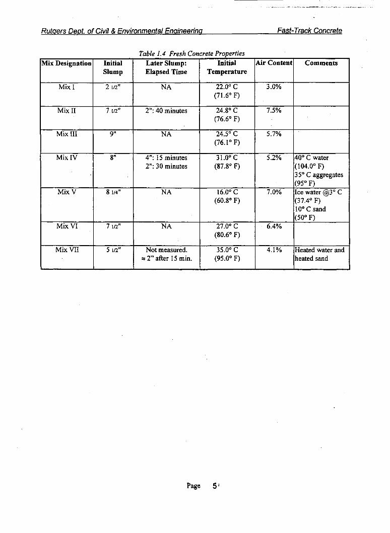
For each mix slump, air content (via pressure method), and initial temperature were taken. When possible, later slumps were taken, after some elapsed time. Details of the fiesh concrete properties are found in Table 1.4.

1 fl. oz/cwt.

18 fl. ozl cwt.

32 fl. ozJcwt.

Page 4

Rutqers Dept. of Civil & Environmental Enaineerina Fast-Track Concrete

Table 1.4 Fresh Concrete Properties Mix Designation Initial Later Slump: Initial Air Content Comments

Slump Elapsed Time Temperature

Mix I 2 In" NA 22.0" c 3.0% (71.6" F)

Mix I1 7 IR" 2": 40 minutes 24.8" C 7.5% (76.6" F)

Mix I11 9ll NA 24.5" C 5.7% (76.1 " F)

Mix IV 8" 4": 15 minutes 31.0" C 5.2% 40" C water 2": 30 minutes (87.8' F) (104.0" F)

35" C aggregates (95" F)

Mix V 8 114'' NA 16.0" C 7.0% Ice water @3" C (60.8' F) (37.4" F)

10" C sand (50' F)

Mix VI 7 1R" NA 27.0" C 6.4% (80.6" F)

Mix VII 5 1R" Not measured. 35.0" C 4.1% Heated water and = 2" after 15 min. (95.0' F) heated sand

Page 51

Rutaers Dept. of Civil & Environmental Enqineerino Fast- Track Concrete

B. Determination of Datum Temperature Datum temperature is most simply described as the temperature below which the rate of cement hydration may be considered negligible. It is necessary to experimentaIly determine the datum temperature for a concrete mix when establishing a correlation between maturity and strength. Incorrect specification of the datum temperature can introduce bias; the strength-maturity relationship may not be universal for all temperatures. Incorrect datum specification, for example, may overestimate the strength of a particular pour if it is substantially colder or warmer than average.

In general, ASTM C 1074 guidelines were followed for the purpose of determining the datum temperature for the fast-track concrete. The ASTM procedure consists of maintaining sets of concrete (or mortar) samples at different (constant) temperatures, then comparing the strength-gain rates of different temperatures graphically to extrapolate the temperature at which the strength-gain rate is zero (or, hydration ceases). The ASTM standard suggests the use of 2" mortar cubes submersed in a temperature-controlled bath. A temperature-controlled bath is employed, rather than air, because the conductive medium is much more effective at maintaining the concrete temperature. The justification for mortar cube samples is that they are sufficiently small so that there is negligible temperature gradient across the sample.

The ASTM procedure was followed, with the exception of the samples used. Rather than mortar cubes, 3" x 6" concrete cylinders were used. It was felt that the use of mortar samples is somewhat "artificial" and is an unnecessary compromise; the final product of this research is concrete, not mortar. Though 2" cubes were not used, the 3" x 6" cylinders are still sufficiently small so that negligible gradient was found across the samples, as measured by embedded temperature probes. The temperature differential between the center of a cylinder and the bath temperature never exceeded 1 " C.

The concrete cylinders were maintained at a constant temperature in a 55 gallon drum of water. The drum was wrapped with a 20' length of electrical heating tape, providing up to 2000 watts of uniform heating to the drum. The heating tape was controlled by a temperature switch. Tkfe temperature was maintained within about 0.5" C of a constant temperature. To assure uniform temperature throughout the drum, compressed air was forced through a filter at the bottom of the drum, aerating and circulating the water.

Five different temperature-controlled baths were used: 22.5" C (72.5' F), 24.4" C (75.9" F), 24.1" C (75.4' F), 32.5' C (90S"F), 10.9"C (51.6"F).

The exDerimenta1 Drocedure was as follows: 1 . After molding the cylinders, the tops were tightly covered with plastic. A temperature probe

was inserted into one cylinder. 2. The cylinders were placed into the bath. The temperature of the bath and one of the

cylinders was continually monitored and the data recorded for a period of 24 hours. 3. Beginning soon after concrete setting, cylinders were removed fiom the bath, usually in

groups of three, for testing. The cylinders were capped with molten s u l k and were tested in compression. Cylinders were typically tested at increasing time intervals. Example: 8 hours, 12 hours, 24 hours, 48 hours, 96 hours, 384 hours.

4. After 24 hours, the bath temperature continued to be controlled for up to 28 days. However, temperature data collection stopped at 24 hours

.

The analytical D I D C ~ ~ U I Z for determining the datum temDerature by the ASTM standard is as follows:

Page 6

Rutuers Dept. of Civil & Environmental Enaineerina Fast-Track Concrete

K-Valua Versus Curing Tempemturn Example of ASTM C1074 Analytical Pmedure For Oetenmining Datum Temperature

0

0 5 10 IS 20 25 30

Curing Tcmprnknm (dcgrea C) . 35 I

I ~

Comrnedts: In this figure, the K-Values, determined in Figure 1.2, are graphed versus the curing temperature. The x-intercept represents a K-value of zero (a rcaction rate of zero). This x-intercept gives a datum tempuahue, for this example, of 1.1 degrees C.

F i w e I .3 Examvle of ASTM CI 074 Procedure for Determining Datum Temwrature

Aoulication of ASTM C1074 Procedure to Fast-Track Concrete As stated previously, the ASTh4 procedure for determining the datum temperature is applicable when the relevant time period is reached in several days. However, for the fast-track concrete, the relevant time period is not reached in several days. It is reached in several hours. Consequently, datum temperature calculations are goJ typical. A graph of the reciprocal of strength versus the reciprocal of age is shown in Figure 1.4. Note that the experimental curves are not straight lines, as they were in Figure 1.2, the example case.

~ _ _ _ _

. . .__- - ..- . . -

Rutuers Dept. of Civil & Environmental Enuineerinu Fast-Track Concrete

K-Values Venus Curing Temperatuns Example of ASTM C1074 Analytical Procedure For Deterimining Datum Temperature

0 6

0

0.5

0.4

- c 3 0.3

z - -

0.2

0.1

0

0 5 10 I5 20

Curing Tcmpcnmre ( d q m u C) .

25 30 35

mments: In this figure, the K-Values, determined in Figure 1.2, are graphed versus the curing temperature. The x-intercept presents a K-value of zero (a reaction rate of zero). This x-intercept gives a datum temperature, for this example, of 1.1 :grees C.

Fiaure I . 3 Examule of ASTM CI 0 74 Procedure for Determining Datum Temverature

ADDlication of ASTM C1074 Procedure to Fast-Track Concrete As stated previously, the ASTM procedure for determining the datum temperature is applicable when the relevant time period is reached in several days. However, for the fast-track concrete, the relevant time period is not reached in several days. It is reached in several hours. Consequently, datum temperature calculations are I& typical. A graph of the reciprocal of strength versus the reciprocal of age is shown in Figure 1.4. Note that the experimental curves are not straight lines, as they were in Figure 1.2, the example case.

Page 8

Rutaers Dept. of Civil & Environmental Enuineerinu Fast-Track Concrete

1 00035

I

0 003

i

I

0 0025

I

I - .

1 ;

a 0002 1 : d

5 00015

- 1 -

0.001

0 0005

0

Reciprocal of Strength Venus Reciprocal of Age: Determining the K-Values forthe Fast-Track Concrete

-%-Mix IV - 32.46 C

0 0.02 0.04 0.06 0.08 0.1 0.12 0.14 0.16 0.18

UAEe (lbomn)

For clarity, mixes I1 and In are not shown

Comments: It is evident that the relationship between the reciprocal of strcngth and the reciprocal of age is non-linear, indicating that the K-values are not constant.

Fiaure 1.4 Reciurocal of Strength Versus Recinroca/ ofAae for the Fast-Track Concrete

From Figure 1.4, it is evident that the K-values are not constant for the f&-track concrete, over time; i.e., the curves are not straight lines. The curves only approach linearity for times exceeding 12 hours at high temperatures, and 48 hours at very lower temperatures.

The implication of K-values that are not constant is that the datum temperature is not constant over time. In fact, the datum temperature decreases over time. At a very early age it may be found that hpiktion only proceeds if the temperasure is quite high. Over time, however, hydration will begin, at an ever decreasing temperature. Eventually, the decrease in the datum temperature becomes insignificant and a constant datum temperature is reached. This time coincides with the portions of Figure 1.4 that are straight lines.

Efforts were made to estimate the manner in which the datum temperature decreases over time, through use of the experimental data. Various functional forms were chosen for the K-values, including exponential and piece-wise linear functions of time. The results were maturity functions where the datum temperature was expressed as afunction of time. However, these maturity functions were

Rutqers Ded. of Civil & Environmental Encrineerinq Fast-Track Concrete

unnecessarily complex and could not be incorporated in standard maturity meters in any way. Consequently, the study of time-dependent datum temperatures was not considered further.

It was concluded that a single datum temperature for the first twelve hours could not be obtained using the ASTM standard.

I 1

Reciprocal of Strength Versus Reciprocal of Age: Determination of K-Values Ibr Fast-Track Mix, Excluding Very Early Ages

0.0006 ,

0 0005

0 0004

- .- a 5, 00003 t

% - - =

I 4 0 0002

I

, 00001

.Mix U - 24.37 C O M i 111 - 24.13 C

x Mi IV - 32.46 c

0 0.01 0.02 0.03 0.04 0.0s 0.06 0.07 0.08 0.09

1/A- ( I h u n ) L

Mix I - 22.48 C Average Cwing Temperature Mix I1 - 24.37OC Average Curing Temperature Slope = 0.006495 Slope = 0.0018516

:ntercept = O.OOO1669 Interupt = 0.000184 C = 0.090131 K = 0.028357 X2 = 0.9414 R2=0.7221

Mix III - 24. I3 O C Average Cauing Temperature Mix N - 32.46 O C Average Curing Tempratwe Slope = 0.0014667 3lope = 0.002264

[ntcrcept = 0.000200 In~t=0.0001821 K = 0.088557 K = 0.124135

R2 = 0.9124 32 = 0.9439 Mix V - 10.91 O C Average Curing Temprazure

Slope = 0.0056927 Intercept = 0.0001945

K = 0.034161 R2 = 0.8546

F i w e 1.5 Determmina the “Long-Term ” K-Valws for the Fast-Track Mi

Rutaers Deot. of Civil & Environmental Enaineerina Fast-Track Concrete

Although the datum temperature cannot be determined for very early age, some estimation of the datum temperature may still be made. Examining Figure 1.4, the data approaches linearity when the reciprocal of age is low (later ages). Therefore, a “long-term” datum temperature could be obtained by considering only the linear portion of the curves found in Figure 1.4. This is done in Figure 1.5. From the K-values determined in Figure 1.5, the “long-term” datum temperature of 3.4” C (38.1’ F) was determined from Figure 1.6.

The datum temperature is relatively high. Datum temperatures that are below 0” C (32.0”F) are more typical (-10” C is a typical assumed datum temperature). In addition, the use of admixtures generally lower the d a m temperature, further. However, a concrete mixture that proceeds at a high rate with excessive temperatures can be expected to lose efficiency, in terms of reaction and crystallization, raising the activation energy, and the corresponding datum temperature. Considering this, a high datum temperature appears to be reasonable.

A high datum temperature implies that the initial concrete temperature must be high, for hydration to begin quickly. Maintaining high concrete temperatures, particularly in cold weather, is likely to be more important with the fast-track mix than with conventional mixes.

K-Values Versus Curing Tempcnture: Datum Temperature of Fast-Track Mi, Exduding Very Earfv Ages

0 14

t 0 I2 0

0

By excluding the v a y early age data points, the computed datum tuqaatm rrflects tbc datum at lata ages, approaching infinity. This datum is only applicabk after about 12 hours elapsed With tbe K-values &tamhd, the long-term datum temperature can be estimated . A best-fit line is made for the five K-values, pmiously computed. From the best-fit lie, the datum tcmperaturr is 3.4’ C (38.1O F)

Fiaure 1.6 Determining the “Long-Term ” Datum Temperatwe Ibr the Fast-Track Concrete

Page 4 4

Rutqers Dept. of Civil & Environmental Enqineenncr Fast-Track Concrete

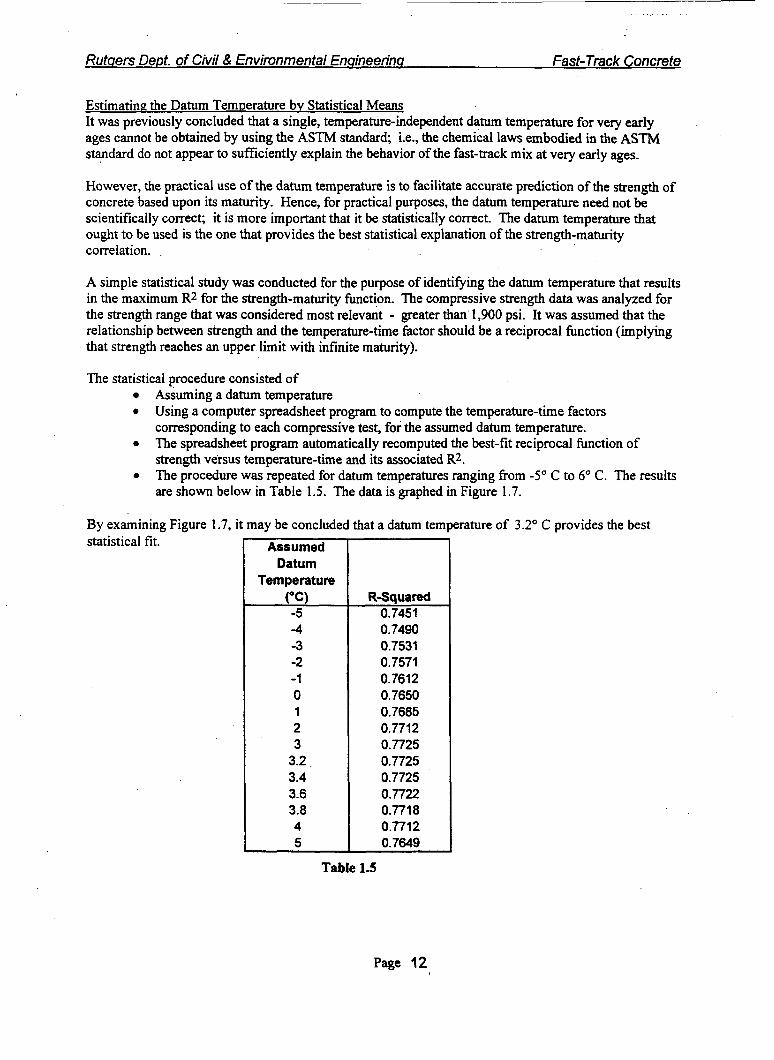
Estimating the Datum Temperature bv Statistical Means It was previously concluded that a single, temperature-independent datum temperature for very early ages cannot be obtained by using the ASTM standard; i.e., the chemical laws embodied in the ASTM standard do not appear to sufficiently explain the behavior of the fast-track mix at very early ages.

However, the practical use of the datum temperature is to facilitate accurate prediction of the strength of concrete based upon its maturity. Hence, for practical purposes, the datum temperature need not be scientifically correct; it is more important that it be statistically correct. The datum temperature that ought to be used is the one that provides the best statistical explanation of the strength-maturity correlation.

A simple statistical study was conducted for the purpose of identifying the datum temperature that results in the maximum R2 for the strength-maturity function. The compressive strength data was analyzed for the strength range that was considered most relevant - greater than 1,900 psi. It was assumed that the relationship between strength and the temperature-time factor should be a reciprocal function (implying that strength reaches an upper limit with infinite maturity).

The statistical procedure consisted of Assuming a datum temperature

0

0

0

Using a computer spreadsheet program to compute the temperature-time factors corresponding to each compressive test, for the assumed datum temperature. The spreadsheet program automatically recomputed the best-fit reciprocal function of strength versus temperature-time and its associated R2. The procedure was repeated for datum temperatures ranging from -5" C to 6" C. The results are shown below in Table 1.5. The data is graphed in Figure 1.7.

By examining Figure 1.7, it may be concluded that a datum temperature of 3.2" C provides the best statistical fit. Assumed

Datum Temperature

("C) -5 -4 -3 -2 -1 0 1 2 3

3.2 3.4 3.6 3.8 4 5

R-Squamd 0.7451 0.7490 0.7531 0.7571 0.7612 0.7650 0.7685 0.7712 0.7725 0.7725 0.7725 0.7722 0.7718 0.7712 0.7649

Table 1.5

Page 12

Rutgers Dept. of Civil and Environmental Engineering Fast-Track Concrete Page 1 13

0.7750

0.7700

0.7650

0.7600

0.7550

0.7500

0.7450

Datum Temperature Versus R' The Statisical R 2 was Computed for Various Assumed Datum Temperatures for the Purpose of

Evaluating the Datum Temperature That Best Fits the Experimental Data

/

- f-urs for 6 equal to 3.2 d e g r e a

/ /

I

-5 -4 -3 -2 -1 0 1 2 3 4 5

Assumed Datum Temperature (degrees C)

Figure 1.7

Rutqers Dept. of Civil & Environmental Ensineennu Fast- Track Concrete

C. Strength - Maturity Correlation

The maturity knction that was chosen was the temperature-timefactor. From ASTM C 1074, the

temperature-time factor is:

M(t) = C (Ta - To) At

Where:

M(t) = the temperature-time factor at age t, in degree C - hours

Ta = average concrete temperature during the time interval At , degrees C

To = datum temperature, degrees C

At = a time interval, in decimal hours

The datum temperature To was taken as 3.2" C (37.8" F), as determined on a statistical basis in Chapter

1B.

Compressive Strength - Temoerature-Time Factor Correlation

A total of 161 compressive strength cylinders from seven mixes were available for strength-maturity

correlation. These cylinders represent curing temperatures ranging from 10.9' C (5 1.6" F) to 68.0' C

(1 54.4' F).

.

Using a datum temperature of 3.2' C (37.8"F), the maturity-compressive strength correlation is as shown

in Figures 1.8 and 1.9. Although the spread of data is quite large for maturities above about 300, the data

showed no correlation with temperature; i.e., manual inspection of the data showed that the residuals

were randomly distributed, independent of temperature. This is particularly encouraging because, as

previously stated, the curing conditions that were included represented all possible temperatures. It may

be concluded that the maturity relationship is valid for all anticipated temperatures.

The compressive strength - temperature-time factor data was best-fit using least-squares regression.

Linear functions were used for temperature-time factors less than 240 and or greater than 7,000 becat&

the data in these ranges most closely resembled a linear function. For the 240 to 7,000 range, a

reciprocal function was used because it is a realistic functional form for a chemical process (see Figure

1.10).

Rutcrers DeDt. of Civil & Environmental Enclineerina Fast-Track Concrete

The best-fit equations for compressive strength versus the temperature-time factor are:

For M < 240: fc = 13.68007M -987.374

For 240 < M < 7,000: (Ufc ) = 0.057066 (1M) + 0.0001 862

for M > 7,000: fc = 0.09636M + 4488.6

Based on the best-fit curve, the target compressive strength of 3,000 psi is reached at a

temperature-time of 388' C-hours, on average (datum of 3.2' C).

Flexural Strength - Temuerature-Time Correlation

A total of (35) 4" x 4" x 14" flexural specimens from six mixes were used. The specimens were tested in

four-point flexure (loads at one-third points) using a universal test machine. Figures 1.1 1 and 1.12 show

the flexural strength versus temperature-time relationship. The flexural strength -maturity data was best-

fit using least-squares regression. A linear function was used for temperature-time factors less than 200

because the data most closely resembled a linear function. A reciprocal function was used for

temperature-time factors greater than 200 because it is a realistic functional form for a chemical process

(Figure 1.13).

The best-fit equations for flexural strength versus maturity are:

For M < 200: fr = 4.8522M-581.8

For M >200: (l&) = 0.305378(1/M) + 0.00161

Based on the best-fit curve, the target flexural strength of 350 psi is reached at a temperature-time

of 245' C-hours, on average (datum of 3.2' C).

Page 15

Rutgers Dept. of Civil and Environmental Engineering Fast-Track Concrete Page 16

8000

7000

6000

5000

4000

3000

2000

I000

0

Compressive Strength Versus Temperature-Time For the Fast-Track Mix Datum Temperature of 3.2" C (37.8' F)

* *

* *

*- _-

lepresents data from compression tests, from seven different mixes -I\--- _-

L 0 5000 10000 15000 20000 25000 30000

Figure 1.8

Rutgers Dept. of 'Civil and Environmental Engineering Fast-Track Concrete Page 17

4500

4000

3 500

3000

2500

2000

1500

1000

500

0 0

Compressive Strength Versus Temperature-Time For Fast-Track Mix: Early Age Datum Temperature of 3.2" C (37.8"F)

100

* * 4

--$ __ f --•

__

200 300 400

Temperature-Time (OC-hours)

500 600

Figure 1.9

Rutgers Dept. of Civil and Environmental Engineering Fast-Track Concrete

.a

k 0.0003

.1

I! a &! 0.0002 .I.1

0.000 I

0

Reciprocal of Compressive Strength Versus Reciprocal of Temperature-Time Factor Datum Temperature of 3.2" C (37.8" F)

. . .-

k

:

I------ __-__

/ I

R Z = 0.77252

0.0005 0.001 0.0015 0.002 0.0025 0.003 0.0035 0.004 0.0045 0.005 0.0055 0.006

lflemperature-Time Factor (1PC-hours) .____

Figure 1.10

Rutgers Dept. of Civil Enviromental Engineering Fast-Track Concrete Page 19

Flexural Strength Versus Temperature-Time For Fast-Track Mix Datum Temperature of 3.2" C (37.8" F)

800

700

600

13 500 B %

3 f 400 iz a

g 300

200

100

0

+

0 2000 4000 6000 8000 10000 I2000 14000 16000 I8000

Temperature-Time ("C - hours)

Figure 1.11

Rutgers Dept. of Civil Enviromental Engineering Fast-Track Concrete Page 20

Flexural Strength Versus Temperature-Time For Fast-Track Mix: Early Age Datum Temperature of 3.2" C (37.8" F)

450

400

350

300

250

l x 2 200 :: 2

I50

I00

50

0

I I

I

I

0 50 100 150 200 250 300 350 400 450

Temperature-Time ("C - hours) -

Figure 1.12

~

~

i I i ! I

1

I 1

I

1

i !

t

I i

I

4 +

b

+

I 4i + +

I I

i

' I I I j i

YI 0 0

0

cy - 0 0 - 2 0 0

VI rn Y) 0 CI

0 0 9 z 8 8 9 s 9

8 0

B 8

v) 0

0 9

10 0

8

s 8

m 0

8

(u 0 z

- 0

8

0

Rutuers DeRt. of Civil & Environmental Enuineerinu Fast-Track Concrete

D. Factored Maturity There are currently two maturity functions in use: equivalent age and temperature-time. The temperature-time factor was the functional form that was used in Chapter 1 .C for correlation with compressive and flexural strength.

In an effort to provide closer fit with the strength data, a new maturity function was used. This maturity function, termed factored maturity, combines aspects of both equivalent age and the temperature-time factor.

0 Temperature-Time, as previously discussed. M(t) = C'(Ta - To) At

Where: M(t) = the temperature-time factor at age t, in degree C - hours Ta = average concrete temperature during the time interval At, degrees C To = datum temperature, degrees C At = a time interval, in decimal hours

Equivalent age, dekned as:

Where: & = equivalent age at a specified temperature Ts (typically 20" C), days or hours. Q = activation energy divided by the gas constant, OK (determined experimentally by the same procedure as for datum temperature). Ta = average temperature of concrete during time interval At, OK. Ts = a specified temperature, OK (typically 20" C) At = time interval, hours e = base of the natural logarithm

Temperature-Time and equivalent age are related concepts. However, there are several key differences: The temperature-time factor, is the simple product of temperature and time. All temperatures are

"the same". A temperature rise of one degree at 50" C results in the same temperature-time factor increase as a one degree rise at 20" C. All temperatures are not "the same" for the equivalent age number. A temperature rise of one degree at 50" C has a stronger impact on equivalent age than a one degree rise at 20" C (due to the

exponential term). Whereas for maturity, hydration ceases at the datum temperature, for equivalent age, hydration never stops. The equivalent age exponential form supposes that hydration occurs at all tempemtures, but the rate decreases exponentially as the temperature drops.

Page 22

Rutaers DeDt. of Civil & Environmental Ensheerins F asf-Track Concrete

0 Due to the difference in functional form, maturity and equivalent age are more likely to provide similar results if the prevalent temperatures are within a narrow range than if the temperatures are widely varying.

Factored Maturity combines aspects of temperature-time and equivalent age. The functional form was developed on the following basis:

The exponentially increasing term used in computing equivalent age, is more realistic for a chemical process where temperatures vary widely, such as in the fast-track mix. The datum temperature concept that is used in the temperature-time factor realistically describes that the concrete will stop reacting if a minimum temperature is not maintained. Equivalent age does not make use of this concept. The hydration process at early ages may be characterized by:

0

0

1. Initially, hydration proceeds very slowly, with a datum temperature, to ', that is very high. Below this high datum temperature, very little activity occm.

2. After some temperature-time factor, Mt is reached, datum temperature drops to its "long- term" level, to. Hydration rate rapidly increases and factored maturity rapidly accrues.

3. High temperatures are more influential than low temperatures. This effect is reflected in an influence factor p.

The basic form of the factored maturity function is as follows:

M' = C (T, - TO)^ At Where:

M' = factored maturity, "C-hours T, = average concrete temperature during time interval At. p = influence facror, increases the relative influence of high temperatures, decreases the relative influence of low temperatures. The factor is scaled to equal unity at 20" C (similar to equivalent age).

To = step-function datwn temperafure. At low maturity7 it is equal to a high datum temperature Once a critical maturity Mt is reached, the datum temperature drops to the long-term datum tempera-

to. To = to ' for M<Mt To=@ forM>Mt M = time-temperature factor with datum temperature of 0" C.

'.

Page 23

Rutqers DeDt. of Civil & Environmental Ensineennu Fast-Track Concrete

Mt = a critical level of maturity. At this level of maturity, the datum temperature drops to its long-term level.

to = later period or long term datum temperature ' = early period datum temperature

The factored maturity function consists of four constants that are determined by a multiple regression technique: the constants are a. Mp tn_', t ~ . The object of the multiple regression was to select the maturity function that results in the best correlation with strength. A reciprocal function was chosen as a logical expression of the relationship between strength and maturity. Plotting the reciprocal of strength versus the reciprocal of factored maturity, the best fit line is the one that minimizes the sum of the squared residuals (this is equivalent to maximizing R2). Iterations were performed with a computer until the values of the four constants were selected that maximized R2. The result was the set of values for the constants:

a = 0.0065 Mt = 9 "C-hoUrs

' = 26" C (78.8" F) to = 3.43" C (38.2" F)

The resulting function describes the hydration process as being very slow, with a datum temperature of 26" C until a temperature-time of 9 "C-hours is reached (this typically occurs after about 20 minutes). Then, the datum drops to 3.43" C and hydration rate rapidly increases.

Figure 1.14 represents the same set of compression samples as Figure 1.10. Note that R2 only increased slightly. It may be concluded that factored maturity offers a correlation with strength that is only marginally better than temperature-time. However, to obtain the best possible correlation, factored maturity was used in the subsequent development of the computer model.

Page 24

Rutgers Dept. of Civil and Environmental Engineering Fast- Track Concrete

Reciprocal of Compressive Strength Versus Reciprocal of Factored Maturity Comparing Wth Figure 7.9, Factored Maturity Exhibits Closer Fit with Strength

--L I . _ _

actored Maturity Function: g= 9 a = 0.0065 f0 = 26' c'

. P

.

I

a

E ?J

P

I O.Ooo3 e 8 u 2 0.0002

0.000 1

0

0.00 1 0.00 15 0.002 0.0025 0.003 0.0035 0.004 0.0045 0.005 0 0.0005

1 I Factored Maturity (degree C-hours)

y = 0.05367~ + 0.0001 8 - R2 = 0.82232

I I

1 Figure I. 14

Rufuers DeDf. of Civil 8, Environmental Enuineerina f asf-Track Concrete

3. Determination of the Heat-Rate Function of the Fast-Track Concrete Mix

Five experiments were carried out for the purpose of obtaining a heat-rate function for the concrete. Heat-rate is the rate at which the internal heat of a concrete mass is increased due to cement hydration. It is well known that the heat-rate of concrete is not constant, but varies over time, typically with peaks associated with rheological changes such as at the time of setting [2]. The heat rate may be functionally related to either time or some measure of maturity. The factored maturity, as previously defined, provided the most consistent relationship over the tested temperature ranges.

Two test apparatus were specifically designed for the purpose of obtaining the heat-rate function.

High-Precision Thermistor Ordinary thennoprobes such as thermocouples provide a resolution and accuracy of about 1°C. For determining the heat-rate it was necessary to have higher resolution temperature measurement. Thermistors were chosen for this purpose. Using a digital ohm-meter, thermistors were individually calibrated. At room temperature, the thermistors used have a resolution of O.OIoC. Six thermistors were connected to a switching unit, wired to a digital ohm-meter. Temperature measurement was carried out manually by recording electrical resistance at time intervals of typically 3 to 10 minutes,

Concrete Calorimeter A large calorimeter wai built, a detail of which is found in Figure 2.1 A plastic drum was filled with 4" to 8" of foam insulation, surrounding a 1 .O ft.3 core. In operation, the 1 .O ft.3 core was filled with concrete, capped with its insulated lid, and sealed shut with silicone. The calorimeter was penetrated with a thermistor probe, embedded in the center of the concrete. The thermistor penetration was also sealed with silicone. This well-insulated vessel simulates the center of a large concrete mass. More importantly, the calorimeter's heat loss is easily calibrated, so that the heat generation caused by the concrete may be precisely known at any point in time.

The calorimeter was calibrated over a period of six days. It was calibrated using water because water is non-reactive, and its thermal properties may easily be related to the thermal properties of concrete, given only its mix proportions [2]. Hot water was placed in the calorimeter. The lid and thermistor penetration were sealed with silicone. Periodically, the temperature inside it was measured, along with the ambient temperature.

A calibration graph is found in Figure 2.2. A least-squares exponential function is fit to the data. To apply this calibration curve to concrete, the specific heat of the mix is assumed to be 028 times the specific heat of water (based on the mix proportions, and assuming the specific heat of aggregate and cement to be 22% of water). Heat loss is assumed to be the same for concrete and water (by conduction, only) so that the temperature loss rate constant for concrete is 3.2 times the rate constant determined for water; i.e., the temperature loss of concrete is about 3.2 times faster than for water.

Test Program Five sets of calorimeter tests were performed. The only variable was initial temperature, varying fkom 16 to 35" C (60.8" F to 95" F). These mixes were designated III, IV, V, VI, W and are the same mixes previously discussed. Temperatures were taken as pviously d e s c r i i for a period of 24 hours following casting.

Page 26

. . _. . . .. .

. . . .

L aJ +-' aJ E

L 0

Q, d

0 U v)

0 z

P, c 4 4

U - a E 3a4 .. 0 U-

5 '.a4

I a -

h

A s I

x v)

L c

r c

/

Rutgers Dept. of Civil and Environmental Engineering Fast- Track Concrete Page 20

45.00

40.00

35.00

G 8 30.00

s 8 25.00

b

r" d a 20.00.

a G

t! e e! 8, 15.00

10.00

5.00

0.00

0

Concrete Calorimeter Calibration Curve

b

- ___ ____ _ _ _ ___.__

figcalorimeter was filled with hot water. For six-days, periodic readings were taken. By computing the derivative of the best-fit exponential function, the temperature-loss rate may be determined, for a given temperature difference. Assuming the specific heat of water to be 3.2 times greater than that of concrete, the temperature loss of concrete is determined to be 3.2 times greater than the corresponding loss for water.

A

20 40 60 80

Time (hours)

I00 * . 120 140

Figure 2.2

RUtg8rS Dept. of Civil and Environmental Engineering Fast-Track Concrete Page 29

___ _ _ _ _ __ - -. - ___ Mix 111 - Initial Temperature 24.5 C - Mix IV - Initial Temperature 31 .O C

. _ _ . __ - -Mix V - Initial Temperature 16.0 C Mix VI - Initial Temperature 27.0 C - - - Mix VII - initial Temperature 35.0 C .

Concrete Temperature Histories For Calorimeter Samples

- - -

70

60

50

G I 40

5 t! E

30

I b

20

10

0

1 I

r---

- ...

\ . --_ -- .-

.. .. .. .

Figure 2.3

Rutaers Dept. of Civil & Environmental Enuineennu Fast-Track Concrete

9.1

9.4

Temperature Rate Data Reduction The temperature-time history for each calorimeter test was obtained. A plot of these temperature-time histories is found in Figure 2.3. At any point on these curves, the slope represents the temperature rate for that instant of time. The slopes of these curves were computed numerically for each data points as the average of the forward and backward tangents. A graphical example of these calculations are given below in Figure 2.4

- -

-

9.8

9.5

Fimre 2.4 Examule of Temoerature Rate Calculations From Twical Temoeratwe-Time PIots

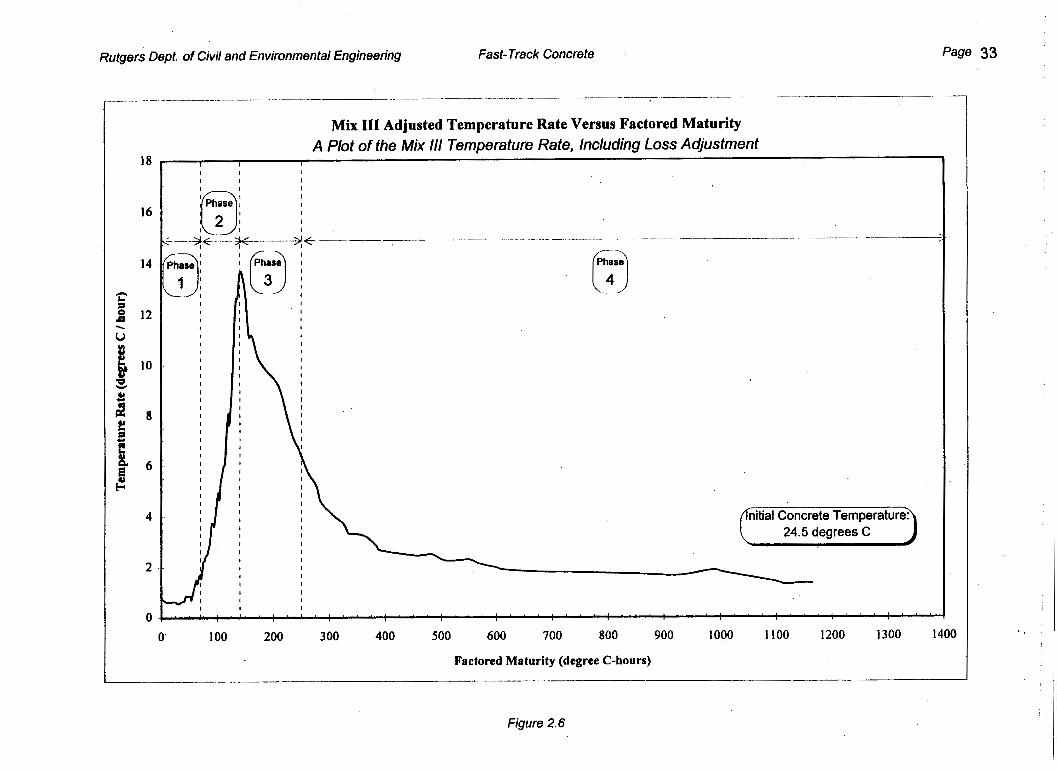
The temperature rates were computed numerically as described in Figure 2.4 and plotted versus the factored maturity (refer to section 1D for the discussion of factored maturity). A temperature rate plot for Mix I11 is given in Figure 2.5.

The temperature rate plot in Figure 2.5 shows two curves: an adjusted curve and an unadjusted curve. The unadjusted curve does not reflect the temperature losses of the calorimeter (note that the temperature rate drops below zero, for this curve). The adjusted curve reflects the calorimeter losses and includes the addition of a loss term. The temperature loss term, as pkviously described, is based on the temperature diference between the outside air and the calorimeter. Knowing the average temperature difference

Rutqers DeRt. of Civil & Environmental Enaineerina Fast-Track Concrete

between the calorimeter and the outside air, along with the corresponding time duration, the temperature change due to losses are easiIy computed. Generally, the adjustment for temperature losses is reflected by an increased temperature rate (a decrease occurs if the concrete is below room temperature). After making the temperature loss adjustments for all time intervals, the adjusted temperature rate versus factored maturity plots are obtained and presented in Figures 2.6,2.7,2.8,2.9,2.10.

Best-Fit Eauations for the Heat Function The computer model requires the temperature rate in the form of continuous functions. While fitting curves to the temperature rate versus factored maturity data, the following items were considered: For a single chemical reaction, the reaction rate is expected to take the following form:

where: rate oc [concentration level] x [e aT]

The exponential term reflects a simplified expression of the Arrhenius Law

And,

a = some constant, dependent on the specific chemical reaction T = the temperature

0

0

The inverse of the factored maturity (1/M ’) is a rough estimate of the concentration level; e.g., the concentration level is zero at an infinite maturity. Although cement hydration is not a single reaction, the functional relationship for reaction rate may be expected to contain the product of (1/M ’) and (e aT), for at least part of its history. Because cement hydration is not a single reaction, the rate may be expected to undergo several distinct phases.

Upon examining the curves of Figures 2.6 through 2.10, it was determined that four distinctphases are present:

1. Factored Maturitv M ’ less than 70” C-hours - hydration rate dips into a “well”. In the factored maturity domain, the data takes the approximate shape of a second-order parabola. Using multiple regression, it was also found that temperature explained a significant portion of the data. The multiple regression functional form that was chosen for this region was:

rate = (AM’* + BM’K) (e aT) From least-squares regression the constants A, B, C, and a were found to be: A = 0.000342734

C = 0.626669857 a = 0.0217301 19 R2 = 0.63027

B=-0.017511043

2. Factored Maturitv M’ between 70’ C-hours and Deak - hydration rate reaches its peak. The multiple regression functional form that was chosen for this region was:

rate = A + ( BM’) (e aT) From least-squares regression the constants A, B, and a were found to be:

B = 0.051846421 a = 0.023953257 R2 = 0.88701

A = -5.534535632

Rutgers Dept. of Civil and Environmental Engineering Fast-Track Concrete

~ Unadjusted Temperature Rate -Adjusted Temperature Rate

__ __ - - - - .- . - __ __ _- -

Page 32

negative, an apparent impossibility. However, that is because the calorimeter loss adjustment is not

_. --________- _ - . - - __ __ _ _ _ _ _ _ ~

Mix 111 Temperature Rate Versus Factored Maturity, With and Without Loss Adjustment Illustrates the Effect of the Adjustment for Calorimeter Loss

\ I

Factored Maturity (degree C-hours) - ~ _ _ _ _ _ ~ _ - _ _ _

Figure 2.5

Rutgers Dept. of Civil and Environmental Engineering Fast- Track Concrete

18

16

14

12

10

8

6

4

2

0

0

3; I I 0

1

I I I I I I I I I I I I I I I I I I I I I I I

Mix 111 Adjusted Temperature Rate Versus Factored Maturity A Plot of the Mix 111 Temperature Rate, Including Loss Adjustment

I I I I I I I I I

0: I I I I I I I

I I I

____ J+-.----- __ - -- - . - __ - _ _ _ _ _

I I 1 I

I I I I I I I I I I I I I I I I

C I

I I I

I I I I I I I I 1 I I I I I I I I I

I I I

nitial Concrete Temperature: c 24.5 degrees C

I I I I I

100 200 300 400 500 600 700 800 900 1000 1100 1200 1300 1400

Factored Maturity (degree C-hours) - ___

Figure 2.6

Rutgers Dept. of Civil and Environmental Engineering Fast- Track Concrete Page 34

18

16

14

12

10

8

6

4

2

0

31 I I

I I I I I I I

Mix IV Adjusted Temperature Rate Versus Factored Maturity A Plot of the Mix /V Temperature Rate, including Loss Adjustment

I I 1

< I I I

I' I

I 31.0 degrees C I I I I I I I I

0 100 200 300 400 500 600 700 800 900 1000 1100 1200 1300 1400

Factored Maturity (degree C-hours) ____ _ _ ~

Figure 2.7

0 - 0 9

0 _ _ 0 m I

0 _ _ 0 2

0 - - 2 - 0 _ _ 0. 2

0 - - 0 OI

0 - - 0 00

0 - - P

P) cn I

i ! z

x 0

Rutgers Dept, of Civil and Environmental Engineering Fast-Track Concrete Page 37

. .

18

16

14

12

10

8

6

4

2

0

9

Mix VII Adjusted Temperature Rate Versus Factored Maturity A Plot of the Mix VII Temperature Rate, Including Loss Adjustment

3; I

I I I I

I I I I I I I I I I I I I I I I I I I I I I I I

I I

I I I I I I I I 1 I I , I I

I

I I nitial Concrete Temperature: I 35.0 degrees C I I I c I

100 200 300 400 500 600 700 800 900 1000 1100 1200 1300 1400

Factored Maturity (degree C-hours)

Figure 2.10

Rutqers Deot. of Civil & Environmental Enuineerins f ast-Track Concrete

3. Factored Maturitv M' between peak and 250" C-hours - In this phase, the rate appears nearly linear in the factored maturity domain. Multiple regression analysis revealed that the data was more influenced by the temperatures of previous periods then current temperature. The resulting expression was:

rate = AM' + (BTI + C) TI = initial concrete temperature

B = 0.2 C = 17.66

A = -0.065 1

4. Factored Maturitv M' greater than 250' C-hours - The multiple regression model is: rate = AM'B

From least-squares regression the constants A, B, and a were found to be: A = 375.79

R* = 0.8065 B = -0.790 1

The actual temperature and factored maturity data was inserted into the predictive equations so that they may be compared with the actual temperature rate data. Figures 2.1 1 to 2.15 show that the predictive equations provide a satisfactory estimation of the temperature rate curves.

I Comparison of Predictive Equatiotu with Experimental Temperature Rate: Mix I11

~

~

I 18000

I 16000

14 ooo

f 12000 . V

f 10000

t

e B :

5:

Y

3 SO00

6000

4.000

2000

0000 0 I00 200 300 400 500 600 100 UIO 900 LOO0 1100 1200 1300 1100

~=-=dMurilr(fke-CI.a)

Figure 2.1 1 ComDarison of Predictive Equations with Exmrimental Temmrature Rate: Mix III

Rutqers Dept. of Civil & Environmental Enqineerina Fast-Track Concrete

Comparison of Predictive Equations with Experimental Temperature Rate: Mix IV

18 000

16.000

I4 000

12.000

10.000

8.000

6 000

4 000

2.000

0.000

0 100 200 300 400 500 600 700 800 900 1000 I100 I200 1300 1400

Fnctored M m t m r i t y (decree C-Lours)

Figure 2.12 Comparison of Predictive Equations with Exuerimental Temuerature Rate: Mix IV

Figure 2.13 Cornoarison of Predictive EQuahons with ExDerirnental TernDerature Rate: Mix V

Page 39

Rutsers Dept. of Civil & Environmental Enuineerinu Fast-Track Concrete

A 'Plot of the Mix VI Actual Temperature Rate and the Predictive Equations

j

- Pred&e Equabons -Aduol Experhnsntsl Data

L

I -- \ j i I

I - !

I

r I Cornoarison of Predictive Epaations with Experimental Tcmper8tore Rate: MU VI

!

I

I I I

I

Figure 2.14 Comuarison of Predictive Eauations with ExDerimental Temuerature Rate: Mix VI

I

Comparison of Predictive Eqnatioar with Experimental Tempemtore Rate: MU VII A Plot of the Mix VIl Actual Temperatun, Rate and the Predictive Equabons

1

i -Pf8fliCUWEqU8tblU -ACUlEXpWhWWO.1.

I

I

I

0 100 200 300 400 SO0 600 700 SW 900 loo0 1100 It00 1300 1400

Factored MaluUy ( & p s C-bur)

Figure 2.15 Cornoarison of Predictive Euuations with Exuerimental TemDerature Rate: Mix W

Page 40

Rutaers DeDf. of Civil & Environmental Enuineerins Fast-Track Concrete

Hvdration Heat Rate The predictive equations satisfactorily estimate the temperature rate of the fast-track mix. To convert this information to the heat of hydration rate, all that is needed is the thermal properties of concrete. Given the mass density of the concrete and an assumed specific heat, c = 880 J k g -“C [3], the heat of hydration is computed by:

q = m c A t Where q = heat of hydration rate (W) m = mass of concrete (kg) c = specific heat (Jkg - “C) At = temperature rate (“Us)

Page 41

Rutuers Dept. of Civil & Environmental Enuineerinu Fast-Track Concrete

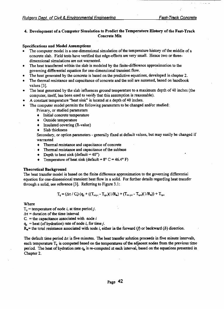
4. Development of a Computer Simulation to Predict the Temperature History of the Fast-Track Concrete Mix

Specifications and Model Assumptions The computer model is a one-dimensional simulation of the temperature history of the middle of a concrete slab. Field tests have verified that edge-effects are very small. Hence two or three- dimensional simulations are not warranted. The heat transferred within the slab is modeled by the finite-difference approximation to the governing differential equation for one-dimensional transient flow. The heat generated by the concrete is based on the predictive equations, developed in chapter 2. The thermal resistance and capacitance of concrete and the soil are assumed, based on handbook values [3]. The heat generated by the slab influences ground temperature to a maximum depth of 40 inches (the computer, itself, has been used to verify that this assumption is reasonable). A constant temperature “heat sink” is located at a depth of 40 inches. The computer model permits the following parameters to be changed andor studied:

Primary, or studied parameters + Initial concrete temperature + Outside temperature + Insulated covering (R-value) + Slab thickness Secondary, or option parameters - generally fvred at default values, but may easily be changed if warranted + Thermal resistance and capacitance of concrete + Thermal resistance and capacitance of the subbase + Depth to heat sink (default = 40”) + Temperature of heat sink (default = 8 O C = 46.4’ F)

Theoretical Background The heat transfer model is based on the finite difference approximation to the governing differential equation for one-dimensional transient heat flow in a solid. For further details regarding heat transfer through a solid, see reference [3]. Refemng to Figure 3.1 :

Where T, = temperature of node i, at time period j. AT = duration of the time interval C, = the capacitance associated with node i q,, = heat (of hydration) rate of node i, for time j. %= the total resistance associated with node i, either in the forward u> or backward (b) direction.

The default time period AT is five minutes. The heat transfer solution proceeds in five minute intervds, each temperature T,, is computed based on the temperatures of the adjacent nodes fiom the previous time period. The heat of hydration rate q,, is re-computed at each interval, based on the equations presented in Chapter 2.

Page 42

Rutqers Dept. of Civil & Environmental Enqineerinq Fast-Track Concrete

Characteristics of Ground Temperatures The initial ground temperature is modeled as a parabolic temperature distribution bounded by a constant temperature heat sink (default setting of 8" C) and the specified surface temperature. Figure 3.2 illustrates this feature. The advantages of this method are:

0

0

The exact temperature distribution of the ground need not be known. A reasonable approximation of the initial ground temperature distribution is made by knowing the ambient (air) temperature. Ground temperature need not be considered as a separate variable Once the simulation begins, heat transfer laws take over, determining the actual temperature distribution through the soil (see Figures 4.4 through 4.6). Therefore, initial errors made in assuming the ground temperature profile are short lived. Field experiments at Rutgers have verified that the temperature at a (default) depth of 40" is very stable and may be reasonably assumed to be about 8" C (46.4O E), during the spring months.

Overview of theoperation of the Computer Simulation The simulation consists of seven blocks, or modules: 1. InDut - This allows the user to change the studied parameters, or opt to change default settings. 2. Element ProDerties - Based on the user input, this module computes the thermal (resistance and

capacitance) and geometric properties of each element - concrete, soil, or insulation. 3 . Initial Ground Temoerature Profile - Based on the input ambient temperature, a heat sink

temperature (default setting = 8" C), a depth to the heat sink (default setting = 40"), and assuming a parabolic temperature distribution, this module computes the starting temperature of each soil element (subsequently, the soil temperature is determined by heat transfer).

4. Heat Generation 8z Factored Maturity - This module continually computes the heat rate of the concrete, based on its factored maturity and temperature. These are typically re-computed at five minute intervals of simulation time. All of this information is stored, for easy recovery, graphical output, etc.

5 . Temperature - Time - This is the core of the simulation. Based on the finite difference approximation to the differential equation for onedimensional transient heat flow, the temperature of each of twelve nodes, representing either concrete or soil, are updated at time intervals (typically five minutes). All of this information is stored.

6. Summary Statistics - This is a database search. It searches the stored information in the Temperature - Time and Heat Generation & Factored Maturity modules, identifying the time at which the target temperature-time product is reached (default = 245' C-hours). This also identifies the peak temperature, and the time at which the peak was reached.

7. Grauhical OutDut - Graphs of the temperature-time history, maturity versus time, and temperature cross-sections of the slab-soil system are automatically generated every time the simulation is run.

Page 43

Rutgers Dept. of Civil and Environmental Engineering Fast- Track Concrete Page 44

-~ ~ .. - _ - ._ -~ _ _ _

Finite Difference Heat Transfer Model for Soil-Slab

. _ _ - ~ @herma/ ropert ties 1 nsulatiofl

k = 0.0288 (W/m - C) c = 700

k = 1.37 (W/m -C) Concrete

c = 880 (Jhg - C) - Soil

k = 1.00 (W/m - C) c = 800 (Jkg - C)

Heat Sink k = infinite c = infinite

Air

Node Numbers Concrete 2

Concrete 3

- - - . - --

_ - -

Concrete 6 -0

Soil 7

Soil 8 ,

.. -0

Soil 9 -0

-_

Soil i i

Heat Sink ___- -_ -0-

equal to the average of adjacent elements.

! Figure 3.1

Rutqers Dept. of Civil & Environmental Enqineerinq fast-Track Concrete

0 -

- -10 -5 - -

0 5 " -15 - =

2 m 2 -20 -

: V 6 : -25 -

f *

-30 .. i!

-35 -

-40

I I I

I I 1 // /! / -Lpp__

~

I

I I I I I

I I

I I

I

I I ~

Page 45

I 0 ~

I

i I I Q -10.

f

z = -15 . 8

z -20. m

a

I: B

14 e -25 -

-30 -

-35

I I I

I I 1 I I

i I

I I I I I

I I

i

-5'\ i I I

I\, I \ I

1 I

l l

I

!

I

, I

I

. . ..

Rutqec; Dept. of Civil & Environmental Encrineerina Fast- Track Concrete

Input alptions Priniary, or Studied Parameters

+ Initial concrete temperature - studied for temperatures ranging from 5 to 35" C (41 to 95" F). + Outside temperature - studied for temperatures ranging from 0 to 35" C (32 to 95" F) + Insulated covering (R-value) - studied for R-values ranging from 0.1 to 20. + Slab thickness - studied for thickness' ranging from 4 to 18 inches

+ Thermal properties of materials may be changed, if justified. Handbook properties were used as default settings: Concrete k (W/m - OC): 1.37

p (kglm3): 2350 Soil (properties of compacted trap rock were approximated) k (W/m - OC): 1.00

p (kglm3): 1900 Insulation k (W/m - OC): 0.0288

p (kg/m3): 15 6 Depth to heat sink may be changed. However, the default setting of 40" is a reasonable

value because field tests and the heat transfer simulation, itself, verifL that negligible influence results at this depth.

6 Temperature of heat sink may be changed. However, the default setting of 8" C is quite reasonable for the spring months.

6 The time increment, AT, may also be changed.

Secondary, or option parameters - generally fixed at default values, but may easily be changed

c (Jikg - OC): 880

c (Jkg - OC): 800

c (Jkg - OC): 700

Page 46

.. . . . ... .~

Rutcrers DePt. of Civil & Environmental Enuineerinu Fast-Track Concrete

5. Use of the Computer Simulation

By changing the input parameters, studies of slab performance may be conducted. Four types of output may be generated: 1.

2.

3.

4.

- Temperature Rate Histories - The computer simulation automatically plots the temperature rate function that was used to simulate the heat of hydration. This plot is an important method of verifying that the simulation is realistic; i.e., for all conditions, the temperature rate function should stil I closely resemble the temperature rate functions determined experimentally. The simulation has been run for over 200 different sets of initial conditions and in all cases, the temperature rate functions have closely resembled the experimental results. - Ternperature Historv and Temperature-Time vs. Time - The computer simulation automatically plots the temperature history of the slab and a plot of Temperature-Time vs. Time. - Ter nr>erature'Cross-Sections - The temperature distribution of the soil-slab system is automatically plo Ted as a function of depth for several points in time. Typically, the temperature cross-sections are generated for two hours elapsed and six hours elapsed. Parametric Study - The performance of the slab is most simply evaluated in terms of the time required to reach some target temperature-time. A parametric study was conducted with a target of 245" C-hours. This target was chosen because it reflects the average temperature-time that corresponds with 350 psi flexural strength. The sensitivity of slab performance was evaluated with respect to changes in four parameters:

Slab Thickness Initial Concrete Temperature Ambient (air) Temperature Insulation R-value

Example Simulation This example illustrates the performance of a slab for a case where ambient conditions are relatively cold. Consequently, the mixing water is heated to produce the highest possible initial concrete temperature. Input: Slab Thickness: 12 inches Initial Concrete Temperature: 25" C (77" F') Ambient Temperature: 10" C (SO" F) Insulation: R = 3.2 (standard insulating blanket for concrete) [4]

Page 47

Rufuers Depf. of Civil & Environmental Endneetinu Fasf-Track Concrete

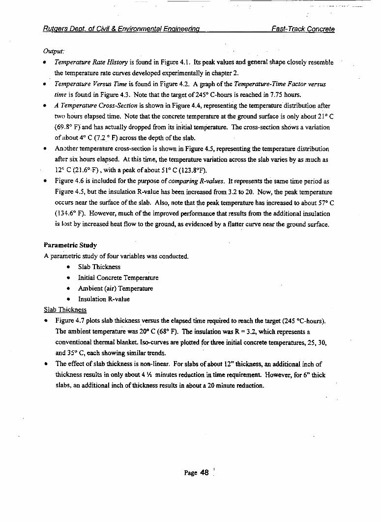
output:

Temperature Rate History is found in Figure 4.1. Its peak values and general shape closely resemble the temperature rate curves developed experimentally in chapter 2. Temperature Versus Time is found in Figure 4.2. A graph of the Temperature-Time Factor versus time is found in Figure 4.3. Note that the target of 245" C-hours is reached in 7.75 hours. A i'kmperahtre Cross-Section is shown in Figure 4.4, representing the temperature distribution after two hours elapsed time. Note that the concrete temperature at the ground surface is only about 2 1 " C (69.8' F) and has actually dropped from its initial temperature. The cross-section shows a variation of about 4" C (7.2 " F) across the depth of the slab. An3ther temperature cross-section is shown in Figure 4.5, representing the temperature distribution aftcr six hours elapsed. At this time, the temperature variation across the slab varies by as much as 12' C (21.6".F), with a peak ofabout 51' C (123.8"F). Figure 4.6 is included for the purpose of comparing R-vahes. It represents the same time period as Figure 4.5, but the insulation R-value has been increased from 3.2 to 20. Now, the peak temperature occurs near the surface of the slab. Also, note that the peak temperature has increased to about 57" C (134.6" F). However, much of the improved performance that results flom the additional insulation is lost by increased heat flow to the ground, as evidenced by a flatter c w e near the ground surface.

Parametric Study A parametric study of four variables was conducted.

Slab Thickness Initial Concrete Temperature Ambient (air) Temperature Insulation R-value

Slab Thickness Figure 4.7 plots slab thickness versus the elapsed time required to reach the target (245 "C-hours). The ambient temperature was 20" C (68" F). The insulation was R = 3.2, which represents a conventional thermal blanket. Iso-curves are plotted for three initial concrete temperatures, 25,30, and 35" C, each showing similar trends. The effect of slab thickness is non-linear. For slabs of about 12" thickness, an additional inch of thickness results in only about 4 'A minutes reduction in time requirement. However, for 6" thick slabs, an additional inch of thickness results in about a 20 minute reduction.

I Page 48

Rutuers Deot. of Civil & Environmental Enaineerina Fast-Track Concrete

Initial Concrete Temperature Figure 4.8 plots the initial concrete temperature versus the time required to reach the target. For this parameter study, the slab thickness was fixed at 12”. The insulation was a conventional thermal blanket. Iso-curves are plotted for seven different ambient temperatures: The initial concrete temperature is extremely influential. For average conditions, a one degree increase in concrete temperature results in about 7 !4 minutes reduction in time requirement. For lower temperatures, the effect is even more pronounced. The increase from 10 to 11 degrees impacts the time requirement by nearly 25 minutes.

Figure 4.9 plots the ambient temperature versus the time required to reach the target, showing five iso-curves for different concrete temperatures. The slab thickness is 12” and the insulation is a conventiona1,thermal blanket. Ambient temperature directly effects the outcome far less than concrete temperature. Figure 4.9 illustrates that, at average temperatures, an increase in ambient temperature reduces the time required by about 5 minutes. However, as discussed earlier and shown in Tables 4.1 and 4.2, ambient temperature has significant indirect effects by lowering the maximum attainable concrete temperature.. Therefore, when combining direct and indirect effects, ambient temperature has the greatest impact of any parameter.

0

Ambient Temuerature

Insulation R-Value Figure 4.10 shows the effect of insulation R-Value on the time required. For ambient temperature of 20’ C, and a 12” thick slab, insulation has a very significant effect for R-values below about 3. Higher R s have negligible impact, for this case. Whereas Figure 4.10 shows the effect of R-Value for a somewhat average case, Figure 4.1 1 shows the effect for an exceptional case. In Figure 4.11, the slab is thinner (8 inches), the ambient temperature is colder (5” C), and the concrete is heated as much as possible. Figure 4.1 1 illustrates that an increase in insulation above that of a conventional thermal blanket may be warranted when slabs are thinner, temperatures are colder, or concrete is significantly warmer than the outside air. An increase in R from 3.2 to 10 can reduce the time required by as much as 40 minutes.

Maximum Attainable Initial Concrete Temperatures The ambient temperature limits the maximum attainable concrete temperature because aggregates and cement cannot normally be heated. Consequently, ambient temperature has both indirect and direct effects on the performance of the concrete: low air temperatures lower the initial concrete temperature and results in higher heat loss to the ground and to the air. Both effects reduce the performance of the concrete. The maximum attainable concrete temperature may be estimated [2] based on the mix proportions, assuming the specific heat of aggregates and cement to be 22% of the specific heat of water. Based on these assumptions, Tables 4.1 and 4.2 provide the maximum attainable concrete temperatures.

Page 49 ‘

Rutgers Dept. of 'Civil and Environmental Engineering Fast- Track Concrete Page'50 ,

18

16

14

12

10

8

6

4

2

0

Computer Simulation of Temperature Rate Versus Factored Maturity

Slab Thickness: 12 inches Insulation R-value: 3.2 (conventional blanket)

0 100 200 300 400 500 600 700 800 900 1000 1100 1200 1300 1400

Factored Maturity (degree C - hours)

Figure 4. I

Fast-Track Concrete Page 51 , Rutgers Dept. of'Civil and Environmental Engineering

80

70

60

50

i 5? 40 e e ii

30 c1

20

10

0

Computer Simulation of Temperature History

-____ I

(ftnitial Concrete Temperature: 25" C (77" F) Air Temperature: lo' C (50" F) Slab Thickness: 12 inches

ulation R-value: 3.2 (conventional blanke

-------

2 4 6 8 10 12 14 16 18 20 22 24 0

Elapsed Time (hours)

- --

Figure 4.2

Page 52 Rutgers Dept. of Civil and Environmental Engineering Fast-Track Concrete

Computer Simulation of Temperature-Time Factor Versus Time

Aitial Concrete Teinperature:' 25" C &" F ) 7 I

400

300 P I 0 a I u c

k

200 z %.

i!

2 k

k 100

0

Elapsed Time (hours)

/

I I I I I I I I I I I I I

I I I I

__t

/A I

I I I I I I I I I I I I I I I I I I I I I

I I I I I

1

A

L

I

/of 245 C-hours reached in 7.75 hours

Figure 4.3

Rutgers Dept. of Civil and Environmental Engineering Fast- Track Concrete Page 53

3 2 c 9 6

12 10 8 6 4 2 0

-2 -4 -6 -8

-10 -12 -14 -16 -18 -20 -22 -24 -26 -28 -30 -32 -34 -36 -3 8 -40

Computer Simulation of Temperature Cross-Section Two Hours Elapsed Time

TOP of Slab

5

(subgrade Temperat-eh

Slab Thickness: 12 inches

Temperature (degrees C) - .-.I__

Figure 4.4

Rutgers Dept. of ,Civil and Environmental Engineering Fast-Track Concrete Page 54

12 10 8 6 4 2 0

-2 -4 -6 -8

-10 -12 -14 -16 -18 -20 -22 -24 -26 -28 -30 -32 -34 -36 -38 -40

Computer Simulation of Temperature Cross-Section Six Hours Elapsed Time

Top of Slab \

Top of Subgrade (bottom of slab) A_, I -1 I I - L , 1 I 1 L . 2 - L - t _ L 1 1 I

5

Slab Thickness: 12 inches

I

Temperature (degrees C)

Figure 4.5

Rutgers Dept. of Civil and Environmental Engineering fast- Track Concrete Page 55

12 10 8 6 4 2 0

-2 -4 -6 -8

-10 -12 -14 -16 -18 -20 -22 -24 -26 -2 8 -30 -32 -34 -36 -38 -40

Computer Simulation of Temperature Cross-Section Six Hours Elapsed Time, Heavily Insulated

Top of Slab

'4- '

Slab Thickness: 12 inches Insulation R-velue: 20

Temperature (degrees C)

Figure 4.6

Rutgers Dept. of Civil and Environmental Engineering Fast-Track Concrete

-_ ~ . . . . . . . . . . . . . . . . . . . . . . . . .. ..... ~~ ..... . .~ _ _

20

18

16

14

12 4 8 10

3

9 F 9 .Y

8 v)

6

4

2

0

.... \ - ...

The Effect of Slab Thickness on the Time Required to Reach Target Strength Computer Simulation Parametric Results

L ----A 1 -~ 1 1. I parget: temperature-time = 245 "C-hours (3.2" C datum$)

\

- ...................

L

__ Initial Concrete Temperature 25 C

- Initial Concrete Temperature 30 C

-Initial Concrete Temperature 35 C

5.5 6 6.5 7 7.5 8 8.5 9 9.5 10 5

Elapsed Time lo Target Strength (hours) _-______ - - - ___

Figure 4.7

Rutgets Dept. of Civil and Environmental Engineering Fast-Track Concrete Page 57

The Effect of Initial Concrete Temperature on the Time Required to Reach Target Strength Computer Simulation Parametric Results

t ' "

Slab Thickness: 12 inches Insulation R-value: 3.2 (conventional blanket) -. I-

I

8 9 10 I I 12 13 14 15 5 6 7

Elapsed Time to Target Strength (hours)

Figure 4.8

Rutgers Dept. of Civil and Environmental Engineering Fast- Track Concrete Page 58

The Effect of Ambient Temperature on the Time Required to Reach Target Strength Computer Simulation Parametric Results

35

30

25

20

15

10

5

0

5 6

- . . . - _ _ -

\, 7

- .

= 245" C-hours (3.2" C datumh

lnsulation R-value: 3.2 (conventional blanket)

';x 8 9 10 1 1 12

Elapsed Time to Target Strength (hours) . . - _ _

13

\ 14

Figure 4.9

Rutgers Dept. of Civil and Environmental Engineering Fast-Track Concrete Page 59

20

18

16

14 n

i; E 12 e 3 10 ai

4J e3 - U

p 8

6

4

2

0

The Effect of Insulation R-Value on the Time Required to Reach Target Strength Computer Simulation Parametric Results

i-

____ -__. - femperature-time = 245 "C-hours (3.2" C datum)

Slab Thickness: 12 20" inches C (68" F)

'---'I-

- Initial Concrete Temperature 25 C

- Initial Concrete Temperature 30 C - Initial Concrete Temperature 35 C

5 5.5 6 6.5 7 7.5 8 8.5 9 9.5 10

Elapsed Time to Target Strength (hours)

Figure 4. I0

Fast-Track Concrete Page 60 Rutgers Dept. of Civil and Environmental Engineering

20

18

16

14

n 8 .g 12

a !J 10 u

E a 8 a Fi

6

4

2

0-1

The Effect of Insulation R-Value on the Time Required: Worst Case Conditions Computer Simulation Parametric Results

I I I I I

f l h p e t h r e - t i t n e = L45' &hours - (3.2" C datum) - -- - - Air Temperature: 5" C (41" F)

[Slab Thickness: 8 inches I--- -

I t--- t---

I

Initial Concrete Temperature 15 C

- Initial Concrete Temperature 20 C - Initial Concrete

J 13 I5 17 19 21 23 25 5 7 9 1 1

Elapsed Time to Target Strength (hours) . ~ _ _ .- - - - . -

Figure 4.11

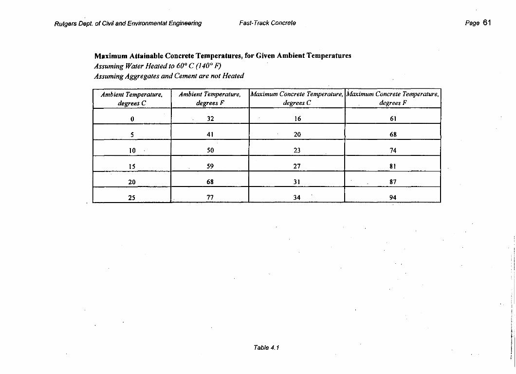
Rutgers Dept. of Civil and Environmental Engineering

Ambient Temperature, Ambient Temperature, Marinium Concrete Temperature, degrees C degrees F degrees C

Fast- Track Concrete

harimurn Concrete Temperature, degrees F

Maximum Attainable Concrete Temperatures, for Given Ambient Temperatures Assuming Water Heated to 60" C (I 40" F) Assuming Aggregates and Cement are not Heated

~

10 ' 50 23 74

15 59 27 81

20 68 31 87

25 77 34 ' 94 1

32 I 16 61

41 20 I 68

Page 61

Table 4.1

Rutgers Dept. of .Civil and Environmental Engineering

Ambient Temperature, Ambieni Temperature, degrees C degrees F

Fast-Track Concrete

Marimum Concreie Temperaiure, degrees C

Maximum Attainable Concrete Temp-ratures, for Given Ambient Temper-tur Assuming Water Heated to 80" C (1 76" F) Assuming Aggregates and Cement are not Heated

0 32 22

10 I 5 41 25

50 29

20

15

68 36 97

59 33

Page 62

S

Maximum Concrete Temperature, I degrees F

84

91

25 77 40 104

Table 4.2

Rutuers Deot. of Civil & Environmental Enuineerinu Fast-Track Concrete

6. Conclusions

Mix Design and Strength Correlation The mix described in this report was based on the mixes researched at NJIT and its design varies very little from those mixes. Several minor modifications were made to the basic NJIT design, none of which are likely to result in significant difference in performance. However, the mixes at the two universities did perform differently and it is believed this is best explained by the differences in cements used. While generally using Essroc cement, NJIT mixes were observed to reach the target strengths at a temperature- time of between 150 and 250 OC-hours. While using Hercules Type I cement, this report finds that the target strengths are reached between 245 (for 350 psi in flexure) and 388 "C-hours (for 3,000 psi in compression) for a datum temperature of 3.2" C (37.8" F). It may be concluded that the Hercules cement requires higher temperatures to reach comparable strengths (whether or not Hercules cement results in higher temperatures has not been addressed).

Despite the different performance of the mixes using Hercules cement, it was found that they still meet the uerformance goals of the Droiect. Using a computer simulation, it was found that the fast-track mix using Hercules cement achieves the target temperature-time of 245 OC-hours (datum of 3.2" C) for a wide range of temperatures and conditions.

.

Some other results: A single datum temperature could not be determined using the ASTM method. The datum temperature was selected as 3.2" C, on a statistical basis; i.e., a datum temperature of 3.2" C provides the best strength-maturity correlation. The correlation of strength with the temperature-time product is valid for all temperatures, exhibiting no apparent bias related to initial or curing temperatures. In an effort to improve the strength correlation, a new functional form for maturity was defined and given the term factored maturity. This functional form showed only marginally better correlation then the temperature-time factor. However, it was used in the development of the computer simulation because the best possible correlation was required.

Determining the Heat Function The variation of the heat of hydration with the factored maturity was determined experimentally. It was found that the rate of temperature increase is closely related to the factored maturity. This temperature rate exhibits four phases, characterized by distinct functional shapes. The temperature-rate curves were analyzed statistically to obtain four equations that describe the heat of hydration of the f&-track mix. By knowing the rate of heat generated, it became possible to develop a heat transfer computer simulation capable of predicting the temperature history of the slab. -

Page 63

. . . . .

Rutclers Deot. of Civil & Environmental Enuineerino Fast-Track Concrete

DeveloDment of a Computer Simulation A computer simulation was developed based on heat transfer principles. The simulation used the experimentally-obtained heat functions and the thermal properties of the soil, slab, and insulation, to calculate the change in temperature of a model slab, over time.

The computer simulation was used for the study of model slabs, varying the thickness, the initial concrete temperature, the air temperature, and the insulation R-value. The results of the parametric study enable recommendations to be made regarding the use of the fast-track mix.

Recommendations The computer simulation enables rational recommendations to made regarding the effects of different slab thickness', the useful temperature ranges of the mix, and the required insulated covering(s).

Slab Thickness Most of the recommendations are intended for 12 inch thick slabs. For slabs that are about 12" thick, a change in thickness of 1" results in only about 4 % minutes change in required time (to reach the target strength). However, for slabs as thin as 6", the effect of a 1" change is about 30 minutes. Slab thickness is critical at low temperatures. In some cases additional insulation may be warranted (see Figure 4.7)

Temperature Table 5.1 summarizes recommendations for initial concrete temperature, given the ambient temperature. Some additional comments:

For average conditions, an increase in concrete temperature of 1" C results in a reduction in required time of 7 % minutes. An increase of 1" F results in a reduction in required time of 4.2 minutes(see Figure 4.8). For average conditions, increase in air temperature of 1" C directly results in a reduction in required time of about 5 minutes (1" F reduces time requirement by 2.8 minutes). Increased air temperature has the additional indirect impact of raking the maximum attainable concrete temperature. Between direct and indirect effects, air temperature is the most influential variable. (see Figure 4.9) Rapid cooling of the slab may occur during finishing and must be considered in cold weather. It is not sufficient that the concrete be poured at a high temperature; it must be at the required temperature at the time the insulation is placed. It has been shown that insulation (up to about R = lo), above a conventional tfiermd blanket, maybe beneficial for colder temperatures or for thin slabs. This may be obtained with foam insulation board or with additional blankets. Concrete temperatures above about 32" C (89.6" F) lose slump very quickly and should be used with caution (see Table 1.4)

Page 64

Rutcrers Dent, of Civil 8, Environmental Enuineerina Fast-Track Concrete

Insulation An insulated covering is a necessity in all temperature conditions. For average conditions, the use of conventional thermal blankets provides sufficient insulation; additional insulation is not required and has negligible impact. However, additional insulation is a beneficial option for the following cases:

Thin slabs, thickness less than about 6" Cold temperatures (about 10 to 15" C, or 50" F to 59" F), all thickness'

Quality Control It has been shown that the size of the concrete pour strongly influences the time requirement; thin slabs require significantly more time to reach the target, than thicker slabs. Size effect has a similar effect on test samples such as cylinders and prisms. Consequently, cylinders and prisms will tend to gain maturity much slower than the slab. For this reason evaluation of in-place strength should follow these procedures:

Decisions regarding in-place strength, such as the re-opening of a roadway, should be based on the target temperature-time factor of 24S0 C-hours in the slab (at 3.2" C datum). Waiting until the target strength is reachedin the test samples is overly conservative. Cylinders and prisms should be tested at or near the target temperatke-time factor of 245" C-hours, to verify its correlation with the target strength. This will necessarily occur afer the slab has reached its target. For subsequent pours, the target temperature-time factor may be modified (if justified) based on the performance of previous jobs.

Rutgers Dept. of Civil and Environmental Engineering

. Minimum Concrete Temperature to Attain Strength in 9 hours

-

Fast-Track Concrete

Comments

Pour not recommended

Table 5.1: Temperature Recommendations Assuming Slab Thickness of 12 inches Assuming Conventional Insulating Blanket (R = 3.2) Target Strength: 35Opsi in Flexure (245" C-hours for 3.2' C datum)

21

' 19

18

Ambient Temperature, degrees C

Heat as warm as possible. Additional insulation optional.

Heating required

Heating required

4 0

-

-

33

10 24

23

22

15

30

20

18

25

30

35 29

17 Heating optional . .

I

Table 5.1 i

Rutcrers Dept. of Civil & Environmental Enuineerinu Fast-Track Concrete

7. References

1. American Society for Testing and Materials, 1991 Annual Book of ASTM Standards. Construction,

2. Mehta, P. Kumar. Concrete: Structure. Prouerties. and Materials, Prentice-Hall, First Edition, 1986. 3. Holman, J.P., Heat Transfer, McGraw-Hill, seventh edition, 1990. 4. American Concrete Institute, ACI Manual of Concrete Practice Part I. 1978, Committee 306, pp. 1-

19.

. Vol. 4.02, 1991,C1074, pp. 544-540.

Page 67 i