Faster Math FunctionsRobin Green – Sony Computer Entertainment Americarobin_green@playstation.sony.com

The art and science of writing mathematical libraries has not been stationary in the past ten years. ManyComputer Science reference books that were written in the 1970’s and 1980’s are still in common use and, asmathematics is universally true, are usually seen as the last word on the subject. In the meantime hardware hasevolved, instruction pipelines have grown in length, memory accesses are slower than ever, multiplies and squareroot units are cheaper than ever before and more specialized hardware is using single precision floats. It is time togo back to basics and review implementations of the mathematical functions that we rely on every day. With a bitof training and insight we can optimize them for our specific game related purposes, sometimes evenoutperforming general purpose hardware implementations.

Measuring Error

Before we look at implementing functions we need a standard set of tools for measuring how good ourimplementation is. The obvious way to measure error is to subtract our approximation from a high accuracyversion of the same function (usually implemented as a slow and cumbersome infinite series calculation). This iscalled the absolute error metric:

approxactualabs fferror −= (1)

This is a good measure of accuracy, but it tells us nothing about the importance of any error. An error of 3 isacceptable if the function should return 38,000 but would be catastrophic if the function should return 0.008. Wewill also need to graph the relative error:

0when1 ≠−= actualactual

approxrel f

ff

error (2)

When reading relative error graphs, an error of zero means there is no error, the approximation is exact. Withfunctions like sin() and cos() where the range is ±1.0 the relative error is not that interesting, but functionslike tan() have a wider range and relative error will be an important metric of success.

Sine and Cosine

For most of the examples I shall be considering implementations of the sine and cosine functions but many of thepolynomial techniques, with a little tweaking, are applicable to other functions such as exponent, logarithm,arctangent, etc.

Resonant Filter

When someone asks you what is the fastest way to calculate the sine and cosine of an angle, tell them you can doit in two instructions. The method, called a resonant filter, relies on having previous results of an anglecalculation and assumes that you are taking regular steps through the series.

int N = 64;float PI = 3.14159265;float a = 2.0f*sin(PI*N);

float c = 1.0f;float s = 0.0f;

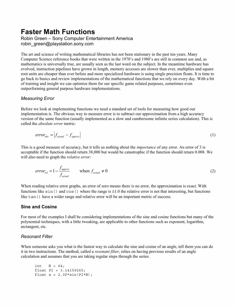
for(i=0; i<N; ++i) { output_sine = s; output_cosine = c; c = c – s*a; s = s + c*a; ...}

Note how the value of c used to calculate s is the newly updated version from the previous line. This formula isalso readily converted into a fixed-point version where the multiplication by a can be modeled as a shift (e.g.multiply by 1/8 converts to a shift right by three places).

–1

–0.5

0

0.5

1

1 2 3 4 5 6 7 8

Figure 1. Resonant filter sine and cosine - 8 iterations over 3π/2

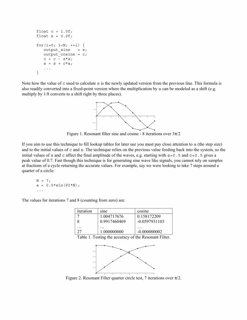
If you aim to use this technique to fill lookup tables for later use you must pay close attention to a (the step size)and to the initial values of c and s. The technique relies on the previous value feeding back into the system, so theinitial values of s and c affect the final amplitude of the waves, e.g. starting with s=0.5 and c=0.5 gives apeak value of 0.7. Fast though this technique is for generating sine wave like signals, you cannot rely on samplesat fractions of a cycle returning the accurate values. For example, say we were looking to take 7 steps around aquarter of a circle:

N = 7;a = 0.5*sin(PI*N);...

The values for iterations 7 and 8 (counting from zero) are:

iteration sine cosine7 1.004717676 0.1581722098 0.9917460469 -0.0597931103… … …27 1.000000000 -0.000000002Table 1. Testing the accuracy of the Resonant Filter.

0

0.2

0.4

0.6

0.8

1

1 2 3 4 5 6 7

Figure 2. Resonant Filter quarter circle test, 7 iterations over π/2.

The end points of this function miss the correct values of 1.0 and 0.0 by quite large amounts (see Figure 2). If,however, we extend the table to generate the whole cycle using 27 samples we find that the final values for s andc are correct to 9 decimal places. Adding more iterations will reduce this error but won’t make it disappear.Clearly this approximation is useful for generating long sequences of sine-like waves, especially over entirecycles, but is not well suited to accurate, small angle work.

Goertzels Algorithm

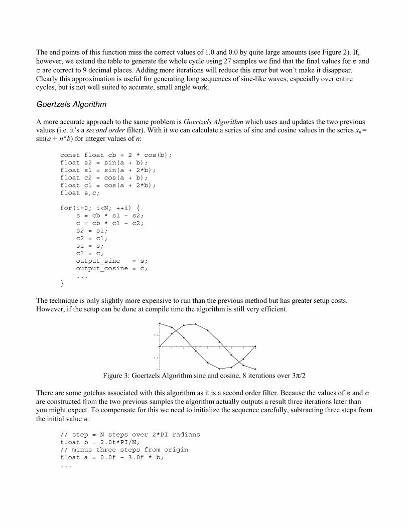
A more accurate approach to the same problem is Goertzels Algorithm which uses and updates the two previousvalues (i.e. it’s a second order filter). With it we can calculate a series of sine and cosine values in the series xn =sin(a + n*b) for integer values of n:

const float cb = 2 * cos(b);float s2 = sin(a + b);float s1 = sin(a + 2*b);float c2 = cos(a + b);float c1 = cos(a + 2*b);float s,c;

for(i=0; i<N; ++i) { s = cb * s1 – s2; c = cb * c1 – c2; s2 = s1; c2 = c1; s1 = s; c1 = c; output_sine = s; output_cosine = c; ...}

The technique is only slightly more expensive to run than the previous method but has greater setup costs.However, if the setup can be done at compile time the algorithm is still very efficient.

–1

–0.5

0

0.5

1

1 2 3 4 5 6 7 8

Figure 3: Goertzels Algorithm sine and cosine, 8 iterations over 3π/2

There are some gotchas associated with this algorithm as it is a second order filter. Because the values of s and care constructed from the two previous samples the algorithm actually outputs a result three iterations later thanyou might expect. To compensate for this we need to initialize the sequence carefully, subtracting three steps fromthe initial value a:

// step = N steps over 2*PI radiansfloat b = 2.0f*PI/N;// minus three steps from originfloat a = 0.0f – 3.0f * b;...

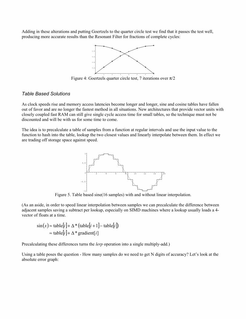
Adding in these alterations and putting Goertzels to the quarter circle test we find that it passes the test well,producing more accurate results than the Resonant Filter for fractions of complete cycles:

0

0.2

0.4

0.6

0.8

1

1 2 3 4 5 6 7

Figure 4: Goertzels quarter circle test, 7 iterations over π/2

Table Based Solutions

As clock speeds rise and memory access latencies become longer and longer, sine and cosine tables have fallenout of favor and are no longer the fastest method in all situations. New architectures that provide vector units withclosely coupled fast RAM can still give single cycle access time for small tables, so the technique must not bediscounted and will be with us for some time to come.

The idea is to precalculate a table of samples from a function at regular intervals and use the input value to thefunction to hash into the table, lookup the two closest values and linearly interpolate between them. In effect weare trading off storage space against speed.

–1

–0.5

0

0.5

1

2 4 6 8 10 12 14 16

Figure 5. Table based sine(16 samples) with and without linear interpolation.

(As an aside, in order to speed linear interpolation between samples we can precalculate the difference betweenadjacent samples saving a subtract per lookup, especially on SIMD machines where a lookup usually loads a 4-vector of floats at a time.

( ) [ ] [ ] [ ]( )[ ] ]gradient[*table

table1table*tablesinii

iiix∆+≈

−+∆+≈

Precalculating these differences turns the lerp operation into a single multiply-add.)

Using a table poses the question - How many samples do we need to get N digits of accuracy? Let’s look at theabsolute error graph:

–0.015

–0.01

–0.005

0

0.005

0.01

0.015

2 4 6 8 10 12 14 16

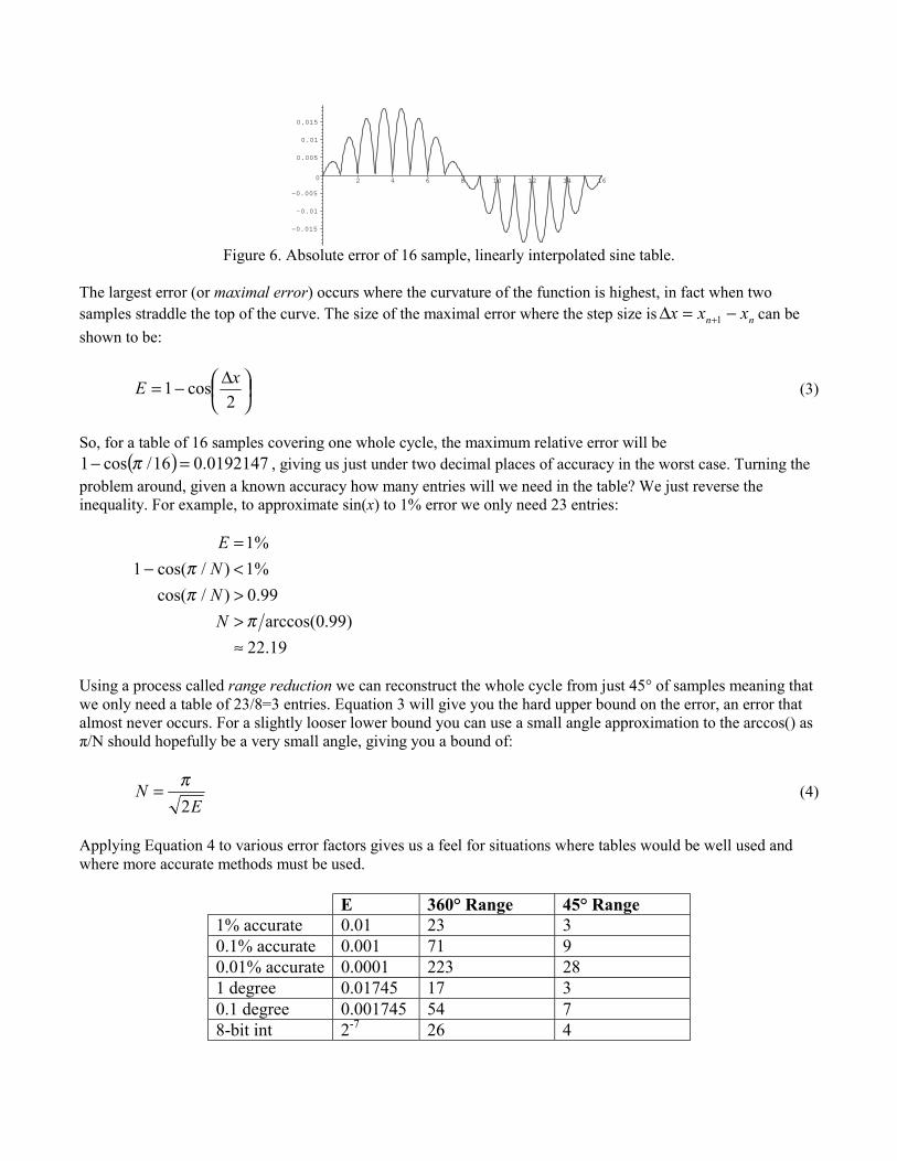
Figure 6. Absolute error of 16 sample, linearly interpolated sine table.

The largest error (or maximal error) occurs where the curvature of the function is highest, in fact when twosamples straddle the top of the curve. The size of the maximal error where the step size is nn xxx −=∆ +1 can beshown to be:

∆−=

2cos1 xE (3)

So, for a table of 16 samples covering one whole cycle, the maximum relative error will be( ) 0192147.016/cos1 =− π , giving us just under two decimal places of accuracy in the worst case. Turning the

problem around, given a known accuracy how many entries will we need in the table? We just reverse theinequality. For example, to approximate sin(x) to 1% error we only need 23 entries:

19.22)99.0arccos(

99.0)/cos(%1)/cos(1%1

≈>><−=

πππ

NNNE

Using a process called range reduction we can reconstruct the whole cycle from just 45° of samples meaning thatwe only need a table of 23/8=3 entries. Equation 3 will give you the hard upper bound on the error, an error thatalmost never occurs. For a slightly looser lower bound you can use a small angle approximation to the arccos() asπ/N should hopefully be a very small angle, giving you a bound of:

EN

2π= (4)

Applying Equation 4 to various error factors gives us a feel for situations where tables would be well used andwhere more accurate methods must be used.

E 360° Range 45° Range1% accurate 0.01 23 30.1% accurate 0.001 71 90.01% accurate 0.0001 223 281 degree 0.01745 17 30.1 degree 0.001745 54 78-bit int 2-7 26 4

16-bit int 2-15 403 5124-bit float 10-5 703 8832-bit float 10-7 7025 88064-bit float 10-17 ~infinite 8.7e+8

Table 2: Size of table needed to approximate sin(x) to a given level of accuracy

Range Reduction and Reconstruction

The sine and cosine functions have an infinite domain. Every input value has a corresponding output value in therange [0…1] and the pattern repeats every 2π units. To properly implement the sine function we need to take anyinput angle and find out where inside the [0..2π] range it maps to. This process, for sine and cosine at least, iscalled additive range reduction.

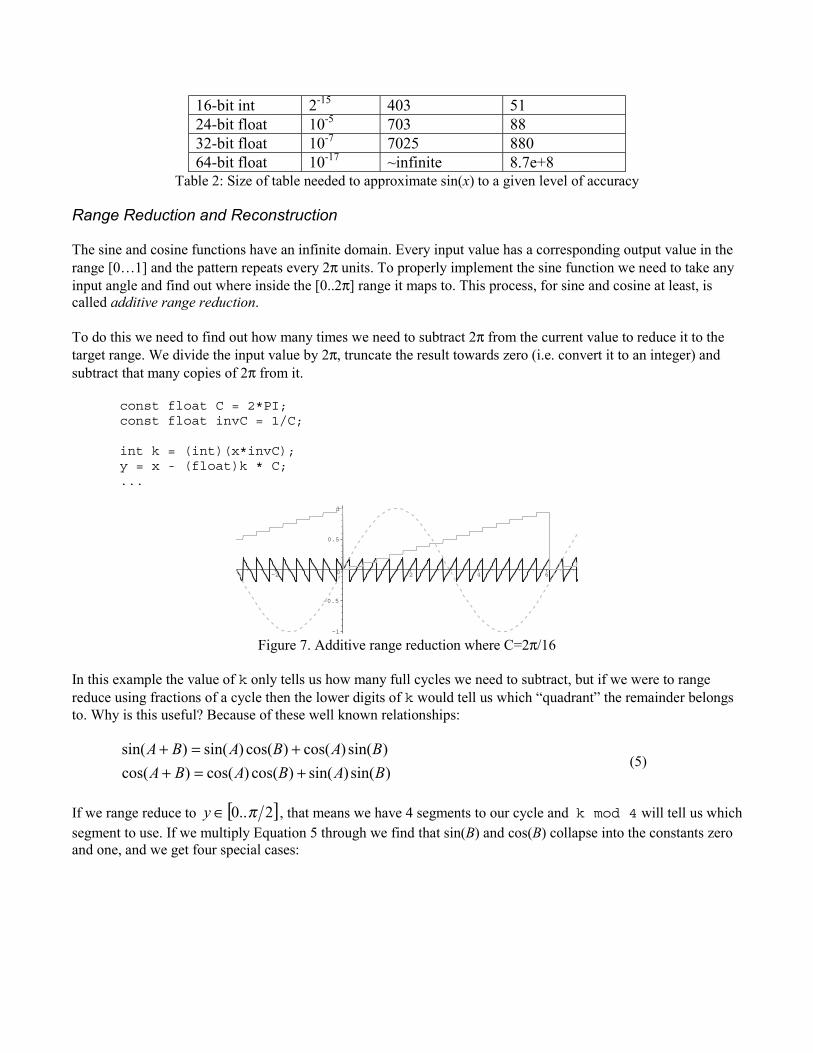
To do this we need to find out how many times we need to subtract 2π from the current value to reduce it to thetarget range. We divide the input value by 2π, truncate the result towards zero (i.e. convert it to an integer) andsubtract that many copies of 2π from it.

const float C = 2*PI;const float invC = 1/C;

int k = (int)(x*invC);y = x - (float)k * C;...

–1

–0.5

0

0.5

1

–2 2 4 6

Figure 7. Additive range reduction where C=2π/16

In this example the value of k only tells us how many full cycles we need to subtract, but if we were to rangereduce using fractions of a cycle then the lower digits of k would tell us which “quadrant” the remainder belongsto. Why is this useful? Because of these well known relationships:

)sin()sin()cos()cos()cos()sin()cos()cos()sin()sin(

BABABABABABA

+=++=+

(5)

If we range reduce to [ ]2..0 π∈y , that means we have 4 segments to our cycle and k mod 4 will tell us whichsegment to use. If we multiply Equation 5 through we find that sin(B) and cos(B) collapse into the constants zeroand one, and we get four special cases:

( )( )( )( ) )sin(2/*3sin

)cos(2/*2sin)cos(2/*1sin)sin(2/*0sin

yyyy

yyyy

−=+−=+

=+=+

ππππ

Leading to code like:

float table_sin(float x) { const float CONVERT = (2.0f * TABLE_SIZE) / PI; const float PI_OVER_TWO = PI/2.0f; const float TWO_OVER_PI = 2.0f/PI;

int k = int(x * TWO_OVER_PI); float y = x – float(k)*PI_OVER_TWO; float index = y * CONVERT; switch(k&3) { case 0: return sin_table(index); case 1: return sin_table(TABLE_SIZE-index); case 2: return -sin_table(TABLE_SIZE-index); default: return -sin_table(index); } return(0); }

Why stop at just four quadrants? To add more quadrants we need reconstruct the final result by to evaluatingEquation 5 more carefully using either inlined constants or a table of values:

...s := sin_table(y);c := cos_table(y);switch(k&15) { case 0: return s; case 1: return s * 0.923880f + c * 0.382685f; case 2: return s * 0.707105f + c * 0.707105f; case 3: return s * 0.382685f + c * 0.923880f; case 4: return c; case 5: return s * -0.382685f + c * 0.923880f; ...}

Note how we have had to approximate both the sine AND cosine in order to produce just the sine as a result. Forvery little extra effort we can easily reconstruct the cosine at the same time and the function that returns them bothfor an input angle, traditionally present in FORTRAN mathematical libraries, is usually called sincos().

You will find that most libraries use the range reduction, approximation and reconstruction phases in the designof their mathematical functions and that this programming pattern turns up over and over again. In the nextsection we will generate an optimized polynomial that replaces the table lookup and lerp.

Polynomial Approximations

People’s first introduction to approximating functions usually comes from learning about Taylor Series at highschool. Using a series of differentials we can show that the transcendental functions break down into an infiniteseries of expressions – e.g.

...!9!7!5!3

)sin(9753

−+−+−= xxxxxx

If we had an infinite amount of time and infinite storage then this would be the last word on the subject. As wehave a very finite amount of time and even less storage, let’s start by truncating the series at the 9th power andmultiplying through (to 5 sig. digits):

975

9753

0000027557.000019841.00083333.016667.0362880

15040

1120

161)sin(

xxxxx

xxxxxx

+−+−=

+−+−≈

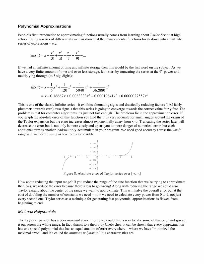
This is one of the classic infinite series - it exhibits alternating signs and drastically reducing factors (1/x! fairlyplummets towards zero), two signals that this series is going to converge towards the correct value fairly fast. Theproblem is that for computer algorithms it’s just not fast enough. The problems lie in the approximation error. Ifyou graph the absolute error of this function you find that it is very accurate for small angles around the origin ofthe Taylor expansion but the error increases almost exponentially away from x=0. Truncating the series later willdecrease the error but is not only is more costly and opens you to more danger of numerical error, but eachadditional term is another load/multiply-accumulate in your program. We need good accuracy across the wholerange and we need it using as few terms as possible.

-0.006

-0.004

-0.002

0

0.002

0.004

0.006

-3 -2 -1 1 2 3

Figure 8. Absolute error of Taylor series over [-π..π]

How about reducing the input range? If you reduce the range of the sine function that we’re trying to approximatethen, yes, we reduce the error because there’s less to go wrong! Along with reducing the range we could alsoTaylor expand about the center of the range we want to approximate. This will halve the overall error but at thecost of doubling the number of constants we need – now we need to calculate every power from 0 to 9, not justevery second one. Taylor series as a technique for generating fast polynomial approximations is flawed frombeginning to end.

Minimax Polynomials

The Taylor expansion has a poor maximal error. If only we could find a way to take some of this error and spreadit out across the whole range. In fact, thanks to a theory by Chebychev, it can be shown that every approximationhas one special polynomial that has an equal amount of error everywhere – where we have “minimized themaximal error”, and it’s called the minimax polynomial. It’s characteristics are:

• For a power N approximation, the error curve will change sign N+1 times.• The error curve will approach the maximal error N+2 times.

The method used to find these polynomial approximations is called the Remez Exchange Algorithm and it worksby generating a set of linear equations, for example:

0)sin( 2 =++− nn cxbxax for a set of values [ ]nmxn ..∈

These are solved to find the required coefficients a,b and c, the maximal error is found and fed back into nx . Thishighly technical optimization problem is sensitive to floating-point accuracy and is difficult to program, so we callon the professionals to do it for us. Numerical math packages like Mathematica and Maple have the necessaryenvironments with the huge number representations and numerical tools needed to give accurate answers.

The arguments needed to calculate a minimax polynomial are:

• the function to be approximated• the range over which the approximation is to be done• the required order of our approximation, and• a weighting function to bias the approximation into minimizing absolute (weight=1.0) or the relative

error.

Let’s find a 7th order polynomial approximation to sin(x) over the range [0..π/4], optimized to minimize relativeerror. We start by looking at the Taylor expansion of sin(x) about x=0, just to get a feel for what the polynomialshould look like. The result shows us that the series has a leading coefficient of 1.0 and uses only the odd powers:

753 980001984126.03008333333301666666670)sin( xx.+x.xx −−≈

A raw call to minimax will, by default, use all coefficients of all available powers to minimize the error leading tosome very small, odd looking coefficients and many more terms than necessary. We will transform the probleminto one of finding the polynomial +++= 2)( cxbxaxP in the expression:

)()sin( 23 xPxxx +≈ (6)

First, we form the minimax inequality expressing our desire to minimize the relative error of our polynomial P:

errorx

xPxxx ≤−−)sin(

)()sin( 23

Divide through by 3x :

error

xx

xPxx

x

≤−−

3

223

)sin(

)(1)sin(

We want the result in terms of every second power, so we substitute 2xy = :

error

yy

yPyy

y

≤−−

2/3

2/3

)sin(

)(1)sin(

And so we have reduced our problem to finding a minimax polynomial approximation to:

( )yy

y 1sin23 − with the weight function ( )y

ysin

23

In order to evaluate the function correctly in the arbitrary precision environments of Mathematica or Maple it isnecessary (ironically) to expand the first expression into a Taylor series of sufficient order to exceed our desiredaccuracy, in order to prevent the specially written arbitrary accuracy sine function from being evaluated:

−+−+−+−62270208003991680036288050401206

1 5432 yyyyy

Our last task is to transform the range we wish to try and approximate. As we have substituted 2xy = , so ourrange [0..π/4] is transformed to [0..π2/16]. Running these through the minimax function looking for a secondorder result gives us:

232000195152806008332160701666665460 y.y.. P(y) −+−=

Resubstituting this result back into Equation 6 gives us the final result:

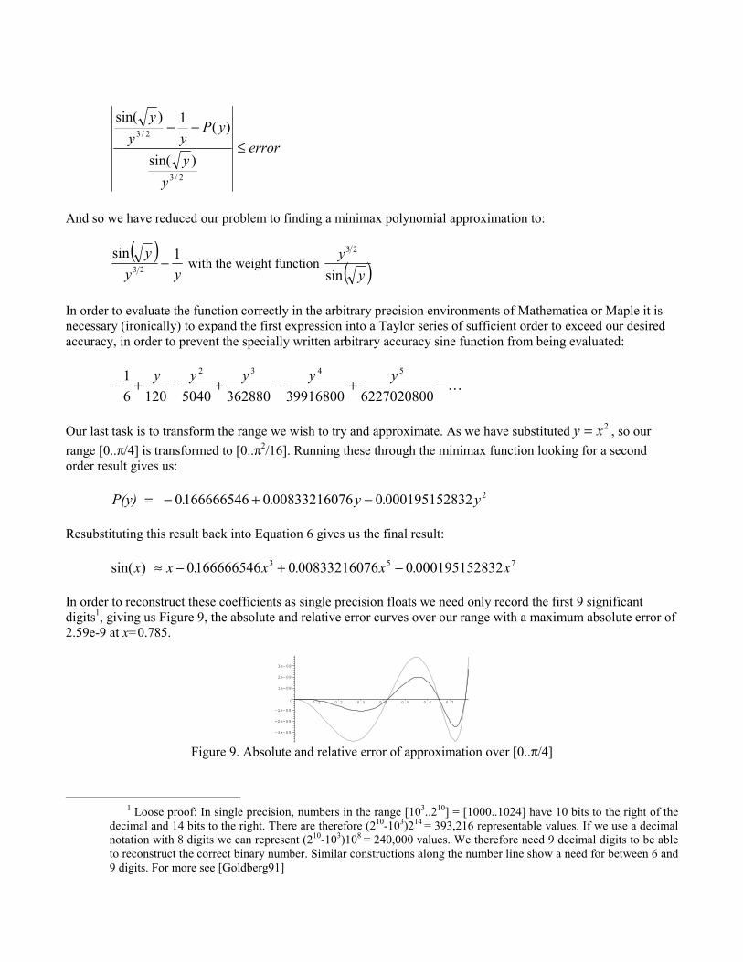
753 32000195152806008332160701666665460)sin( x.x.x.x x −+−≈

In order to reconstruct these coefficients as single precision floats we need only record the first 9 significantdigits1, giving us Figure 9, the absolute and relative error curves over our range with a maximum absolute error of2.59e-9 at x=0.785.

–3e–09

–2e–09

–1e–09

0

1e–09

2e–09

3e–09

0.1 0.2 0.3 0.4 0.5 0.6 0.7

Figure 9. Absolute and relative error of approximation over [0..π/4]

1 Loose proof: In single precision, numbers in the range [103..210] = [1000..1024] have 10 bits to the right of the

decimal and 14 bits to the right. There are therefore (210-103)214 = 393,216 representable values. If we use a decimalnotation with 8 digits we can represent (210-103)108 = 240,000 values. We therefore need 9 decimal digits to be ableto reconstruct the correct binary number. Similar constructions along the number line show a need for between 6 and9 digits. For more see [Goldberg91]

Optimizing for Floating Point

The same technique we used to remove a coefficient can be used to force values to machine representable values.Remember that values like 1/10 are not precisely representable using a finite number of binary digits. We canadapt the technique above to force coefficients to be our choice of machine-representable floats. Rememberingthat all floating point values are rational numbers, we can take the second coefficient and force it to fit in a singleprecision floating point number:

0015625000073255920410.166666562

279620124 −=−=k

Now we have our constant value, let’s optimize our polynomial to incorporate it. Start by defining the form ofpolynomial we want to end up with:

)()sin( 253 xPxkxxx ++=

Now we form the minimax inequality:

errorx

xPkkxxx ≤−−−)sin(

)()sin( 253

Which, after dividing by x5, substituting y=x2 and solving for P(y) shows us that we have to calculate the minimaxof:

( )yk

yyy

+− 22/51sin

with weight function ( )yy

sin

2/5

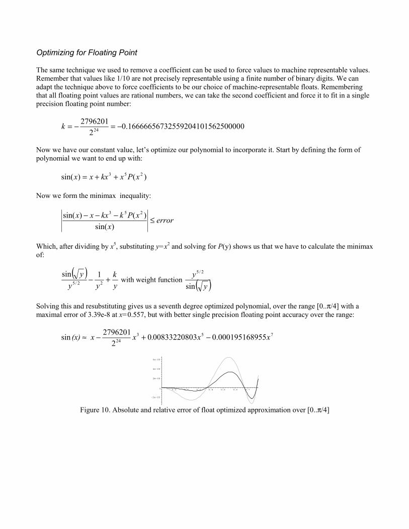
Solving this and resubstituting gives us a seventh degree optimized polynomial, over the range [0..π/4] with amaximal error of 3.39e-8 at x=0.557, but with better single precision floating point accuracy over the range:

75324 550001951689.0300833220800

22796201sin xx.x x(x) −+−≈

–2e–09

0

2e–09

4e–09

6e–09

0.1 0.2 0.3 0.4 0.5 0.6 0.7

Figure 10. Absolute and relative error of float optimized approximation over [0..π/4]

Evaluating Polynomials

The fast evaluation of polynomials using SIMD hardware is a lecture in itself, but there are three main methods ofgenerating fast sequences of operations – Horner form, Estrins Algorithm and brute force searching.

When presented with a short polynomial of the form:

y = ax2 + bx + c

Most programmers will write code that looks like this:

y = a*x*x + b*x + c; // 3 mults, 2 adds

For the case of a small polynomial this isn’t too inefficient, but as polynomials get bigger the inefficiency of thistechnique becomes painfully obvious. Take for example a 9th order approximation to sine:

y = x + // 24 mults, 4 adds a*x*x*x + b*x*x*x*x*x + c*x*x*x*x*x*x*x + d*x*x*x*x*x*x*x*x*x ;

Clearly there has to be a better way. The answer is to convert your polynomial to Horner Form. A Horner Formequation turns a polynomial expression into a nested set of multiplies, perfect for machine evaluation usingmultiply-add instuctions:

z = x*x; y = ((((z*d+c)*z+b)*z+a)*z+1)*x; // 6 mults, 4 adds

Or alternatively using four-operand MADD instructions:

z = x*x; // 2 mults, 4 madds y = d; y = y*z + c; y = y*z + b; y = y*z + a; y = y*z + 1; y = y*x;

Horner form is the default way of evaluating polynomials in many libraries, so much so that most polynomials areusually stored as an array of coefficients and sent of a Horner Form evaluation function whenever they need to beevaluated at a particular input value. Problem is that many computers don’t provide 4-operand MADDinstructions, they accumulate into a register instead. Also the process is very serial with later results relying on theoutput of all previous instructions. We need to parallelise the evaluation of polynomials.

Estrin’s Algorithm

Estrin’s Algorithm works by dividing the polynomial into a tree of multiply-adds and evaluating each expressionat level of the tree in parallel. The best way is to illustrate it is to build up a high power polynomial from firstprinciples. First, let’s break down a cubic expression into sub-expressions of the form Ax+B (NOTE: to make thiseasier to extend I shall be lettering the coefficients backwards, so a is the constant term):

( )( ) )(2

233

abxxcdxabxcxdxxp+++=

+++=

Building a table of higher and higher order polynomials shows regular patterns:

p0(x) = a p1(x) = (bx+a) p2(x) = (c)x2+(bx+a) p3(x) = (dx+c)x2+(bx+a) p4(x) = (e)x4+((dx+c)x2+(bx+a)) p5(x) = (fx+e)x4+((dx+c)x2+(bx+a)) p6(x) = ((g)x2+(fx+e))x4+((dx+c)x2+(bx+a)) p7(x) = ((hx+g)x2+(fx+e))x4+((dx+c)x2+(bx+a)) p8(x) = (i)x8+(((hx+g)x2+(fx+e))x4+((dx+c)x2+(bx+a))) p9(x) = (jx+i)x8+(((hx+g)x2+(fx+e))x4+((dx+c)x2+(bx+a))) p10(x)= ((k)x2+(jx+i))x8+(((hx+g)x2+(fx+e))x4+((dx+c)x2+(bx+a))) p11(x)= ((lx+p)x2+(jx+i))x8+(((hx+g)x2+(fx+e))x4+((dx+c)x2+(bx+a)))

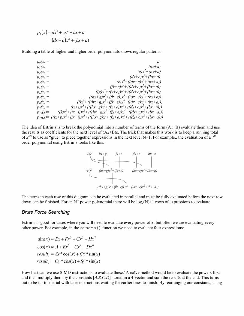
The idea of Estrin’s is to break the polynomial into a number of terms of the form (Ax+B) evaluate them and usethe results as coefficients for the next level of (Ax+B)s. The trick that makes this work is to keep a running totalof x2N to use as “glue” to piece together expressions in the next level N+1. For example,. the evaluation of a 7th

order polynomial using Estrin’s looks like this:

hx+g fx+e dx+c bx+a(x)2

(x2)2 (hx+g)x2+(fx+e)

x4((hx+g)x2+(fx+e)) +((dx+c)x2+(bx+a))

(dx+c)x2+(bx+b)

The terms in each row of this diagram can be evaluated in parallel and must be fully evaluated before the next rowdown can be finished. For an Nth power polynomial there will be log2(N)+1 rows of expressions to evaluate.

Brute Force Searching

Estrin’s is good for cases where you will need to evaluate every power of x, but often we are evaluating everyother power. For example, in the sincos() function we need to evaluate four expressions:

)sin(*)cos(*)sin(*)cos(*

)cos()sin(

2

1

642

753

xSyxCyresultxCxxSxresult

DxCxBxAxHxGxFxExx

+=+=

+++≈+++≈

How best can we use SIMD instructions to evaluate these? A naïve method would be to evaluate the powers firstand then multiply them by the constants [A,B,C,D] stored in a 4-vector and sum the results at the end. This turnsout to be far too serial with later instructions waiting for earlier ones to finish. By rearranging our constants, using

more registers and timing the pipeline intelligently, we can parallelise much of the evaluation as demonstrated bythis fragment of PS2 VU code:

coeff1 = [A, A, E, E]coeff2 = [B, B, F, F]coeff3 = [C, C, G, G]coeff4 = [D, D, H, H]in0 = [x, ?, ?, ?]in2 = [?, ?, ?, ?]in4 = [?, ?, ?, ?]in6 = [?, ?, ?, ?]out = [0, 0, 0, 0]

adda.xy, ACC, coeff1, vf0mulax.zw, ACC, coeff1, in0mulx.zw, coeff2, coeff2, in0mulx.zw, coeff3, coeff3, in0mulx.zw, coeff4, coeff4, in0mulx.x, in2, in0, in0mulx.x, in4, in2, in2mulx.x, in6, in2, in4maddax.xyzw, ACC, coeff2, in2maddax.xyzw, ACC, coeff3, in4maddx.xyzw, out, coeff4, in6

One way to generate rearrangements like this is to evaluate the polynomials using a program made to generate asmany trees of options as possible. For large polynomials (e.g. 22nd order polynomials needed for full doubleprecision arctangents) the number of possibilities is enormous but the calculation only needs a “good answer” andcan be left to cook overnight or even distribute the work across an entire office worth of computers. Thistechnique has been used with good results by Intel in designing their IA64 math libraries [Story00].

A Note On Convergence

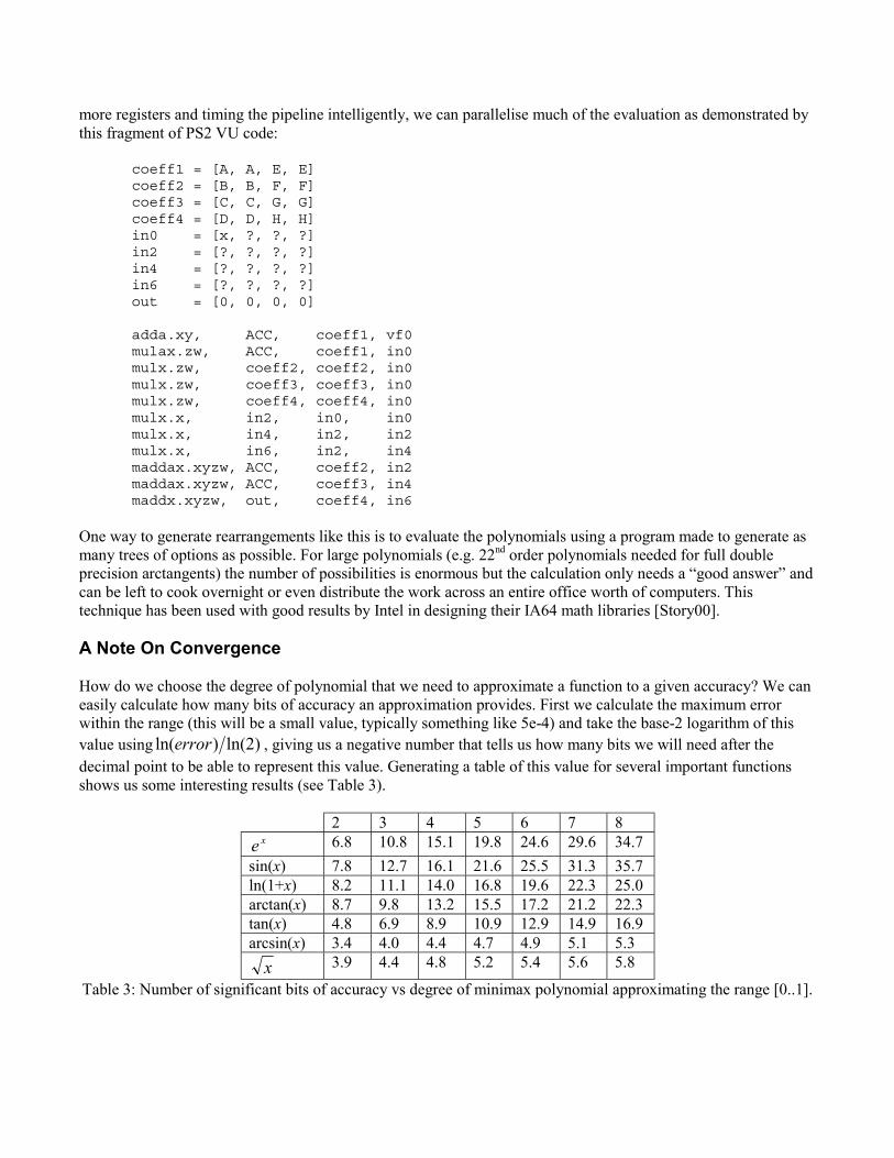
How do we choose the degree of polynomial that we need to approximate a function to a given accuracy? We caneasily calculate how many bits of accuracy an approximation provides. First we calculate the maximum errorwithin the range (this will be a small value, typically something like 5e-4) and take the base-2 logarithm of thisvalue using )2ln()ln(error , giving us a negative number that tells us how many bits we will need after thedecimal point to be able to represent this value. Generating a table of this value for several important functionsshows us some interesting results (see Table 3).

2 3 4 5 6 7 8xe 6.8 10.8 15.1 19.8 24.6 29.6 34.7

sin(x) 7.8 12.7 16.1 21.6 25.5 31.3 35.7ln(1+x) 8.2 11.1 14.0 16.8 19.6 22.3 25.0arctan(x) 8.7 9.8 13.2 15.5 17.2 21.2 22.3tan(x) 4.8 6.9 8.9 10.9 12.9 14.9 16.9arcsin(x) 3.4 4.0 4.4 4.7 4.9 5.1 5.3

x 3.9 4.4 4.8 5.2 5.4 5.6 5.8

Table 3: Number of significant bits of accuracy vs degree of minimax polynomial approximating the range [0..1].

Firstly it shows how well we can use polynomials to approximate exp(x) and sin(x) as each additional power givesus pretty much four bits of accuracy. For a 24-bit single precision floating point value we will only need a sixth orseventh power approximation. The table also shows how badly sqrt(x) is approximated by polynomials as eachadditional power only adds half a bit of accuracy - this is why there are no quick and easy approximations to thesquare root and we must use range reduction with Newtons algorithm and good initial guesses to calculate it.Another surprise is tan(x), after all it’s only )cos()sin( xx isn’t it? Rational functions like this are not wellapproximated by ordinary polynomials and require a different toolkit of techniques.

Tangent

The tangent of an angle is mathematically defined as the ratio of sine to cosine:

)cos()sin()tan(

xxx =

which, when wrapped with a test for 0)cos( =x returning BIGNUM, is a good enough method for infrequent uselike setting up a camera FOV. It is however expensive as range reduction on x happens twice plus a large amountof polynomial evaluation, even if we use sincos() to get both values we still have a division to deal with. Let’slook into coding up a specific function for the tangent using minimax polynomials. Looking at the speed-of-convergence table (Table 3) shows that we are going to have to use more terms than for sine or cosine, so the tanfunction will be more expensive for the same level of accuracy. The question is how many more terms will weneed? That depends on how far we can reduce the input range.

Range Reduction

Thinking back to high school trigonometry, you may recall learning a set of less than enthralling trig identities.Now we can finally see what they are for:

( )θθ tan)tan( −=−

So we can make all input values positive and restore the sign at the end. We have halved our input range. Thenext identity

( ) ( )θπθπ

θ −=−

= 2cot2tan

1tan

Tells us two things – the range –π/2.. π/2 is repeated over and over again. More subtly it also tells us that there isa sweet spot at π/4. As the tangent increases from 0 to π/4, the cotangent decreases from π/2 down to π/4 – so weonly need to approximate the range [0.. π/4] and can flip the functions as we go. Given that the range reduction isalready subtracting multiples of π/4 all we need do is, if the quadrant is odd, subtract one more π/4 from the inputrange:

( )( )( )( )

<≤−<≤<≤−<≤

=

πθπθθθθπθθθ

θ

π

ππ

ππ

π

43

43

2

24

4

iff 2taniff cot

iff 2cot0 iff tan

tan

There is another school of thought that maintains that evaluating either the tangent or cotangent as a largerpolynomial over the [0.. π/2] range, allowing more parallelism in evaluating the polynomial but saving on theserialized range reduction. There are problems with generating minimax polynomials of that size but it has beenused with success.

Polynomial Approximation

In order to form the minimax polynomial approximation to tan in the range [0.. π/2] first let’s look at the TaylorExpansion:

( ) +x+x+x+xx+ x283562

31517

152

3tan

9753

≈

It seems that the polynomial rises in powers of two and starts with x, leading us to use the familiar minimax form:

)()tan( 23 xPxxx +≈

Following the steps for approximating sine replacing sin() for tan() we end up with the minimax inequality:

( )yy

y 1tan23 − with weight ( )y

ytan

23

over [0.. π2/16]

which produces polynomials like:

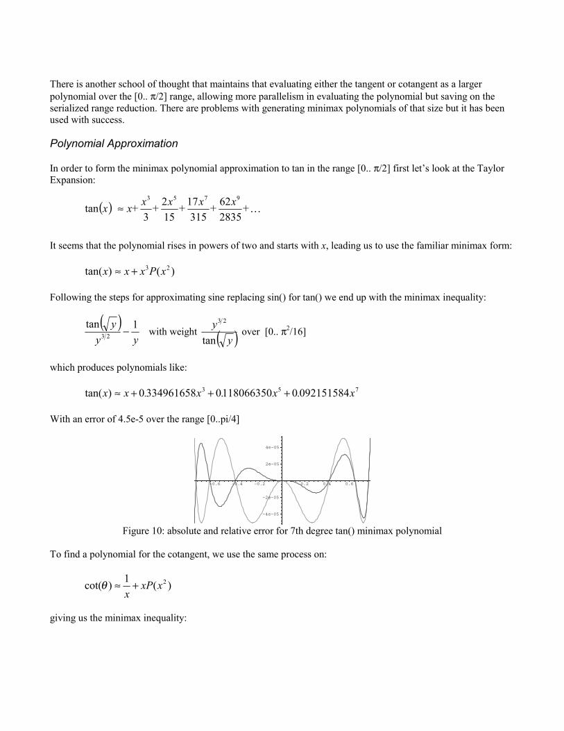
753 092151584011806635003349616580)tan( x.x.x.xx +++≈

With an error of 4.5e-5 over the range [0..pi/4]

–4e–05

–2e–05

2e–05

4e–05

–0.6 –0.4 –0.2 0.2 0.4 0.6

Figure 10: absolute and relative error for 7th degree tan() minimax polynomial

To find a polynomial for the cotangent, we use the same process on:

)(1)cot( 2xxPx+≈θ

giving us the minimax inequality:

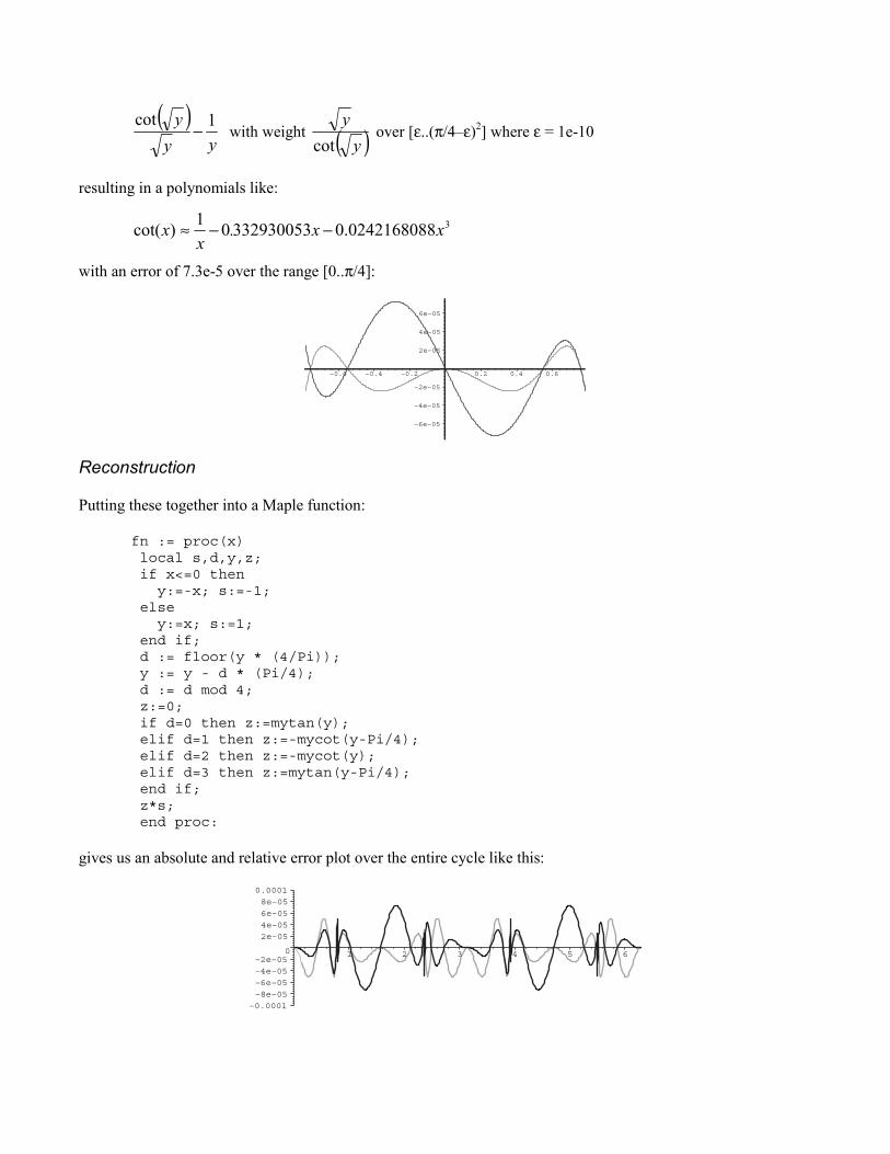
( )yy

y 1cot− with weight ( )y

ycot

over [ε..(π/4–ε)2] where ε = 1e-10

resulting in a polynomials like:

30242168088.033293005301)cot( xx.x

x −−≈

with an error of 7.3e-5 over the range [0..π/4]:

–6e–05

–4e–05

–2e–05

2e–05

4e–05

6e–05

–0.6 –0.4 –0.2 0.2 0.4 0.6

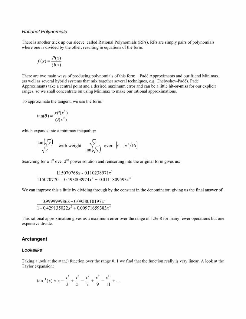
Reconstruction

Putting these together into a Maple function:

fn := proc(x) local s,d,y,z; if x<=0 then y:=-x; s:=-1; else y:=x; s:=1; end if; d := floor(y * (4/Pi)); y := y - d * (Pi/4); d := d mod 4; z:=0; if d=0 then z:=mytan(y); elif d=1 then z:=-mycot(y-Pi/4); elif d=2 then z:=-mycot(y); elif d=3 then z:=mytan(y-Pi/4); end if; z*s; end proc:

gives us an absolute and relative error plot over the entire cycle like this:

–0.0001–8e–05–6e–05–4e–05–2e–05

0

2e–054e–056e–058e–05

0.0001

1 2 3 4 5 6

Rational Polynomials

There is another trick up our sleeve, called Rational Polynomials (RPs). RPs are simply pairs of polynomialswhere one is divided by the other, resulting in equations of the form:

)()()(

xQxPxf =

There are two main ways of producing polynomials of this form – Padé Approximants and our friend Minimax,(as well as several hybrid systems that mix together several techniques, e.g. Chebyshev-Padé). PadéApproximants take a central point and a desired maximum error and can be a little hit-or-miss for our explicitranges, so we shall concentrate on using Minimax to make our rational approximations.

To approximate the tangent, we use the form:

)()()tan( 2

2

xQxxP≈θ

which expands into a minimax inequality:

( )( ) [ ]16over

ytany

weight with tan 2πε

yy

Searching for a 1st over 2nd power solution and reinserting into the original form gives us:

x. + x. .x.x - .

42

3

0111809593049380897401507077011102389710150707681

−

We can improve this a little by dividing through by the constant in the denominator, giving us the final answer of:

42

3

30097165938042913502201095801019709999999860

x.x.x.x.

+−−

This rational approximation gives us a maximum error over the range of 1.3e-8 for many fewer operations but oneexpensive divide.

Arctangent

Lookalike

Taking a look at the atan() function over the range 0..1 we find that the function really is very linear. A look at theTaylor expansion:

+−+−+−≈−

119753)(tan

1197531 xxxxxxx

shows us that as x tends towards zero then atan(x) tends to x, so a reasonable first approximation would be:

xx ≈− )(tan 1

The error on the linear approximation is not so good but, by altering the slope we can improve the result quitedramatically:

baxx +≈− )(tan 1

Solving this equation with minimax over the range [0..1] gives us:

x.+.(x) 78539816400355508730tan 1 ≈−

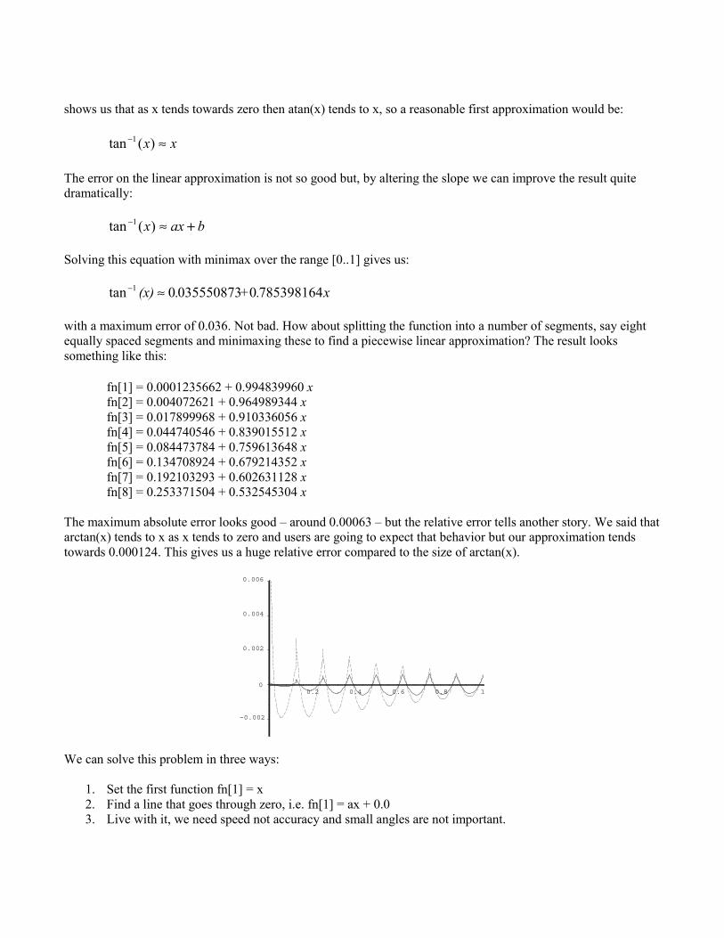
with a maximum error of 0.036. Not bad. How about splitting the function into a number of segments, say eightequally spaced segments and minimaxing these to find a piecewise linear approximation? The result lookssomething like this:

fn[1] = 0.0001235662 + 0.994839960 xfn[2] = 0.004072621 + 0.964989344 xfn[3] = 0.017899968 + 0.910336056 xfn[4] = 0.044740546 + 0.839015512 xfn[5] = 0.084473784 + 0.759613648 xfn[6] = 0.134708924 + 0.679214352 xfn[7] = 0.192103293 + 0.602631128 xfn[8] = 0.253371504 + 0.532545304 x

The maximum absolute error looks good – around 0.00063 – but the relative error tells another story. We said thatarctan(x) tends to x as x tends to zero and users are going to expect that behavior but our approximation tendstowards 0.000124. This gives us a huge relative error compared to the size of arctan(x).

–0.002

0

0.002

0.004

0.006

0.2 0.4 0.6 0.8 1

We can solve this problem in three ways:

1. Set the first function fn[1] = x2. Find a line that goes through zero, i.e. fn[1] = ax + 0.03. Live with it, we need speed not accuracy and small angles are not important.

To calculate option 2 we need generate the minimax inequality:

)()arctan( xxPn +≈θ

Which gives us:

( )( )

810over

arctaneight with warctan

xn

xn-

xx

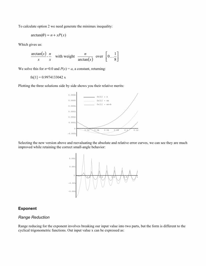
We solve this for n=0.0 and P(x) = a, a constant, returning:

fn[1] = 0.9974133042 x

Plotting the three solutions side by side shows you their relative merits:

–0.0001

0

0.0001

0.0002

0.0003

0.0004

0.0005

0.0006

0.02 0.04 0.06 0.08 0.1 0.12

fn[1] = x

fn[1] = ax

fn[1] = ax+b

Selecting the new version above and reevaluating the absolute and relative error curves, we can see they are muchimproved while retaining the correct small-angle behavior:

–0.002

–0.001

0

0.001

0.002

0.2 0.4 0.6 0.8 1

Exponent

Range Reduction

Range reducing for the exponent involves breaking our input value into two parts, but the form is different to thecyclical trigonometric functions. Out input value x can be expressed as:

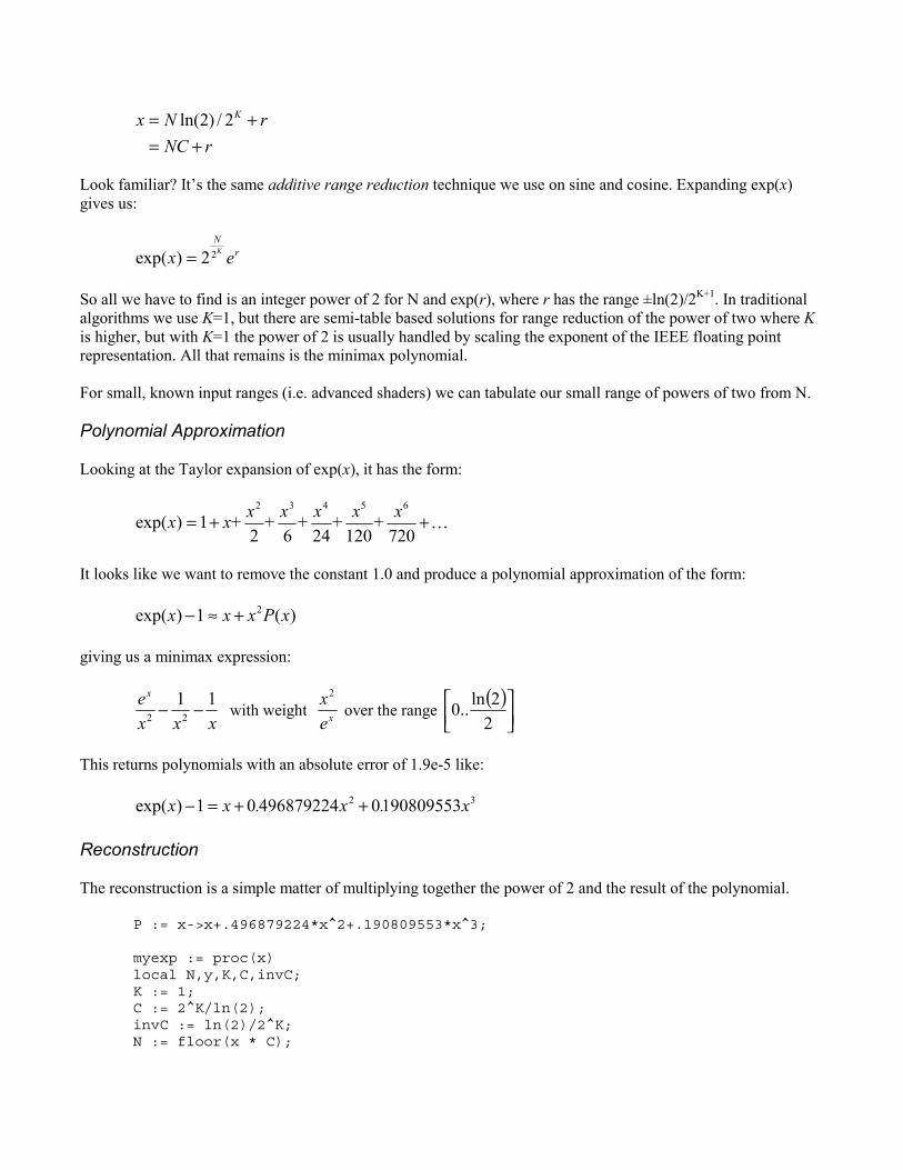
rNCrNx K

+=+= 2/)2ln(

Look familiar? It’s the same additive range reduction technique we use on sine and cosine. Expanding exp(x)gives us:

rN

ex K22)exp( =

So all we have to find is an integer power of 2 for N and exp(r), where r has the range ±ln(2)/2K+1. In traditionalalgorithms we use K=1, but there are semi-table based solutions for range reduction of the power of two where Kis higher, but with K=1 the power of 2 is usually handled by scaling the exponent of the IEEE floating pointrepresentation. All that remains is the minimax polynomial.

For small, known input ranges (i.e. advanced shaders) we can tabulate our small range of powers of two from N.

Polynomial Approximation

Looking at the Taylor expansion of exp(x), it has the form:

++=7201202462

1)exp(65432 x+x+x+x+xx+x

It looks like we want to remove the constant 1.0 and produce a polynomial approximation of the form:

)(1)exp( 2 xPxxx +≈−

giving us a minimax expression:

xxxex 11

22 −− with weight xex2

over the range ( )

22ln..0

This returns polynomials with an absolute error of 1.9e-5 like:

32 190809553049687922401)exp( x.x.xx ++=−

Reconstruction

The reconstruction is a simple matter of multiplying together the power of 2 and the result of the polynomial.

P := x->x+.496879224*x^2+.190809553*x^3;

myexp := proc(x)local N,y,K,C,invC;K := 1;C := 2^K/ln(2);invC := ln(2)/2^K;N := floor(x * C);

y := x-N*invC;2^(N/2^K) * (P(y)+1);end proc:

This algorithm gives a very uninteresting relative error plot, so we’ll skip it…

Conclusion

The task of writing low accuracy mathematical functions using high accuracy techniques has not been covered inany depth in the literature, but with the widespread use of programmable DSPs, vector units, high speed yetlimited hardware and more esoteric shading models, the need to write your own mathematical functions isincreasingly important.

Introductions to polynomial approximation always start by saying how accurate they can be, and this obsessionwith accuracy continues through to extracting the very last bit of accuracy out of every floating point number. Butwhy? Because if you can build high accuracy polynomials with less coefficients, you can also build tiny, lowaccuracy approximations using the same techniques. The levels of accuracy you can obtain with just twoconstants and range reduction can be amazing. Hopefully this article has given you the confidence to grab a mathpackage and generate some of your own high speed functions.

References

[Cody80] Cody & Waite, Software Manual for the Elementary Functions, Prentice Hall, 1980[Crenshaw00] Crenshaw, Jack W, Math Toolkit for Real-Time Programming, CMP Books, 2000[DSP] The Music DSP Source Code Archive online at http://www.smartelectronix.com/musicdsp/main.php[Goldberg91] Goldberg, Steve, What Every Computer Scientist Should Know About Floating Point Arithmetic,

ACM Computing Surveys, Vol.23, No.1, March, 1991 available online fromhttp://grouper.ieee.org/groups/754/

[Hart68] Hart, J.F., Computer Approximations, John Wiley & Sons, 1968[Moshier89] Moshier, Stephen L., Methods and Programs for Mathematical Functions, Prentice-Hall, 1989[Muller97] Muller, J.M., Elementary Functions: Algorithms and Implementations, Birkhaüser, 1997[Ng92] Ng, K.C., Argument Reduction for Huge Arguments: Good to the Last Bit, SunPro Report, July 1992[Story00] Story, S and Tang, P.T.P, New Algorithms for Improved Transcendental Functions on IA-64, Intel

Report, 2000[Tang89] Tang, Ping Tak Peter, Table Driven Implementation of the Exponential Function in IEEE Floating Point

Arithmetic, ACM Transactions on Mathematical Software, Vol.15, No.2, June, 1989[Tang90] Tang, Ping Tak Peter, Table Driven Implementation of the Logarithm Function in IEEE Floating Point

Arithmetic, ACM Transactions on Mathematical Software, Vol.16, No.2, December, 1990[Tang91] Tang, Ping Tak Peter, Table Lookup Algorithms for Elementary Functions and Their Error Analysis,

Proceedings of 10th Symposium on Computer Arithmetic, 1991[Upstill90] Upstill, S., The Renderman Companion, Addison Wesley, 1990