Faster Quantum Chemistry Simulation on Fault-Tolerant Quantum Computers

CitationJones, N. Cody, James D. Whitfield, Peter L. McMahon, Man-Hong Yung, Rodney Van Meter, Alán Aspuru-Guzik, and Yoshihisa Yamamoto. 2012. Faster quantum chemistry simulation on fault-tolerant quantum computers. New Journal of Physics 14(11): 115023.

Published Versionhttp://dx.doi.org/10.1088/1367-2630/14/11/115023

Permanent linkhttp://nrs.harvard.edu/urn-3:HUL.InstRepos:10384783

Terms of UseThis article was downloaded from Harvard University’s DASH repository, and is made available under the terms and conditions applicable to Other Posted Material, as set forth at http://nrs.harvard.edu/urn-3:HUL.InstRepos:dash.current.terms-of-use#LAA

Share Your StoryThe Harvard community has made this article openly available.Please share how this access benefits you. Submit a story .

Accessibility

Faster quantum chemistry simulation on fault-tolerant quantum computers

This article has been downloaded from IOPscience. Please scroll down to see the full text article.

2012 New J. Phys. 14 115023

(http://iopscience.iop.org/1367-2630/14/11/115023)

Download details:

IP Address: 140.247.48.44

The article was downloaded on 28/01/2013 at 16:56

Please note that terms and conditions apply.

View the table of contents for this issue, or go to the journal homepage for more

Home Search Collections Journals About Contact us My IOPscience

Faster quantum chemistry simulation onfault-tolerant quantum computers

N Cody Jones1,7, James D Whitfield2,3,4, Peter L McMahon1,Man-Hong Yung2, Rodney Van Meter5, Alan Aspuru-Guzik2

and Yoshihisa Yamamoto1,6

1 Edward L Ginzton Laboratory, Stanford University, Stanford, CA 94305-4088,USA2 Department of Chemistry and Chemical Biology, Harvard University,12 Oxford Street, Cambridge, MA 02138, USA3 NEC Laboratories, America, 4 Independence Way, NJ 08540, USA4 Physics Department, Columbia University, 538 W 120th Street, New York,NY 10027, USA5 Faculty of Environment and Information Studies, Keio University, Japan6 National Institute of Informatics, 2-1-2 Hitotsubashi, Chiyoda-ku,Tokyo 101-8430, JapanE-mail: ncodyjones@gmail.com

New Journal of Physics 14 (2012) 115023 (35pp)Received 9 April 2012Published 27 November 2012Online at http://www.njp.org/doi:10.1088/1367-2630/14/11/115023

Abstract. Quantum computers can in principle simulate quantum physicsexponentially faster than their classical counterparts, but some technical hurdlesremain. We propose methods which substantially improve the performanceof a particular form of simulation, ab initio quantum chemistry, on fault-tolerant quantum computers; these methods generalize readily to otherquantum simulation problems. Quantum teleportation plays a key role inthese improvements and is used extensively as a computing resource. Toimprove execution time, we examine techniques for constructing arbitrary gateswhich perform substantially faster than circuits based on the conventionalSolovay–Kitaev algorithm (Dawson and Nielsen 2006 Quantum Inform. Comput.6 81). For a given approximation error ε, arbitrary single-qubit gates can be

7 Author to whom any correspondence should be addressed.

Content from this work may be used under the terms of the Creative Commons Attribution-NonCommercial-ShareAlike 3.0 licence. Any further distribution of this work must maintain attribution to the author(s) and the title

of the work, journal citation and DOI.

New Journal of Physics 14 (2012) 1150231367-2630/12/115023+35$33.00 © IOP Publishing Ltd and Deutsche Physikalische Gesellschaft

2

produced fault-tolerantly and using a restricted set of gates in time which isO(log ε) or O(log log ε); with sufficient parallel preparation of ancillas, constantaverage depth is possible using a method we call programmable ancilla rotations.Moreover, we construct and analyze efficient implementations of first- andsecond-quantized simulation algorithms using the fault-tolerant arbitrary gatesand other techniques, such as implementing various subroutines in constant time.A specific example we analyze is the ground-state energy calculation for lithiumhydride.

Contents

1. Introduction 22. Fault-tolerant phase rotations 5

2.1. Phase kickback . . . . . . . . . . . . . . . . . . . . . . . . . . . . . . . . . . 52.2. Gate approximation sequences . . . . . . . . . . . . . . . . . . . . . . . . . . 72.3. Programmable ancilla rotation . . . . . . . . . . . . . . . . . . . . . . . . . . 82.4. Analysis of a single-qubit phase rotation . . . . . . . . . . . . . . . . . . . . . 9

3. Simulating chemistry in second-quantized representation 103.1. Controlled phase rotations . . . . . . . . . . . . . . . . . . . . . . . . . . . . 133.2. Finite precision in pre-calculated integrals . . . . . . . . . . . . . . . . . . . . 133.3. Jordan–Wigner transform using teleportation . . . . . . . . . . . . . . . . . . 153.4. Resource analysis for ground-state energy simulation of lithium hydride . . . . 17

4. Simulating chemical structure and dynamics in first-quantized representation 194.1. Quantum variable rotation . . . . . . . . . . . . . . . . . . . . . . . . . . . . 214.2. Improved parallelism in potential energy operator . . . . . . . . . . . . . . . . 244.3. Resource analysis for first-quantized molecular simulations . . . . . . . . . . . 25

5. Comparing simulation methods 276. Conclusions 29Acknowledgments 30Appendix A. Methods for calculating resources 30Appendix B. Transforming the phase kickback register 31Appendix C. Quantum circuits for potential and kinetic energy operators in first-

quantized molecular Hamiltonians 31References 32

1. Introduction

Simulating quantum physics from first principles is arguably one of the most importantapplications of a quantum computer—a problem intractable to solve in many cases, yet valuableto science [1]. The objective of quantum simulation is to model natural physical systems withHamiltonians that permit a compact representation [2, 3]. Several different applications of aquantum physics simulator have been proposed, including: spin glasses [4] and lattices [5, 6];Bardeen–Cooper–Schrieffer Hamiltonians [7, 8]; and quantum chemistry [9, 10]. More recently,Jordan et al [11] proposed a variant of this approach for simulating relativistic quantum fieldtheories. In this investigation, we narrow our focus to quantum chemistry problems such as

New Journal of Physics 14 (2012) 115023 (http://www.njp.org/)

3

calculating the eigenvalues of a molecular Hamiltonian [9, 12–14]. We aim to demonstrateconstructively how quantum computers can simulate chemistry with an efficient use of resourcesby representing the molecular system with a first-principles Hamiltonian consisting of kineticenergy and Coulomb potential operators between electrons and nuclei. In doing so, we indicatehow close the field of quantum information processing is to solving novel problems for lesscomputational cost than a classical computer.

The motivation behind our study is that in order for computational physics on quantumcomputers to be useful as a scientific tool, it must have an efficient implementation. Oftengeneral algorithmic complexity such as ‘polynomial time’ is taken as a by-word for efficient, butwe go deeper to show the substantial performance disparities between different polynomial-timealgorithms, revealing which ones are significantly less costly in space and time resources thantheir peers. By introducing algorithmic improvements and making quantitative analysis of theresource costs, we show that simulating quantum chemistry is feasible in a practical executiontime. An example problem we analyze is calculating the ground-state energy of lithium hydride(LiH) in 5.6 h on a hypothetical fault-tolerant quantum computer with an execution timeper error-corrected gate of 1 ms. This stands in contrast to previous results based on slowermethods [6], which would require 3.8 years to complete the same task on the same machine.

Quantum chemistry and band structure calculations account for up to 30% of the compu-tation time used at supercomputer centers [15], and ab initio chemistry is one of the twophysics-simulation applications which dominate the use of supercomputing resources (theother being fusion-energy research). The most-employed techniques include density functionaltheory and polynomially tractable approximate quantum chemistry methods [16]. Despite thesuccess of these methods, for example, in simulating the dynamics of a small protein fromfirst principles [17] or in predicting novel materials [18], they are still approximate, and muchwork is carried out in developing more accurate methods. Quantum simulators offer a freshapproach to quantum chemistry [19] as they are predicted to allow for the exact simulation(within a selected basis) of a chemical system in polynomial time. A quantum computer of asufficient size, say 128 logical quantum bits [9, 20], would already outperform the best classicalcomputers for exact chemical simulation. This would open the door to high-quality ab initio datafor parameterizing force fields for molecular dynamics [21] or understanding complex chemicalmechanisms such as soot formation [22], where a number of different chemical species must becompared. This tends to suggest that computational chemistry would be one of the first novelapplications of universal quantum computers.

Several possible simulators have been proposed and studied [19, 23–26], but we focus onfault-tolerant circuit-model quantum simulation in this investigation [2, 6, 9, 10, 14, 20, 27,28]. The reasons for these constraints are straightforward: quantum computers will probablybe sensitive to noise and other hardware errors, thus requiring fault tolerance [29], and fault-tolerant quantum computing has been most successfully applied in the circuit model. Faulttolerance requires an additional overhead for the quantum computer; error correcting codesand the mechanisms they use to correct errors have been studied previously [29–31]. We focushere on another matter critical to simulation algorithms, which is making arbitrary fault-tolerantgates. Arbitrary quantum operations, such as a single-qubit rotation of arbitrary angle aroundthe σ z axis on the Bloch sphere, are typically constructed using a sequence of primitive error-corrected gates [30, 32, 33]. Quantum simulation depends sensitively on the execution time ofarbitrary gates of this form, so one of the core contributions of this paper is to demonstrateefficient constructions for such gates, which would allow simulation of more complex systems

New Journal of Physics 14 (2012) 115023 (http://www.njp.org/)

4

U(τ)U(2 τ)k-2U(2 τ)k-1

. . .

. . .

t (k-1)

0 {t (k-2)

t (0)

. . .

Initialize

State Preparation:

0 {Initialize

State Preparation:

QFT

. . .QFT

. . .

Readout

Figure 1. Schematic of a digital quantum simulation algorithm for energyeigenvalue estimation [2, 9]. The three main steps are state preparation, simulatedevolution, and readout; this investigation focuses on the middle process. Afterpreparing an initial state |ψ0〉, the system is evolved in simulated time by solvingthe time-dependent Schrodinger equation. Note the system propagators U(2xδt)are controlled by qubits in a register representing simulated time. A quantumFourier transform (QFT) on the time register provides an estimate of an energyeigenvalue. The accuracy of the simulation depends on suppressing errors in bothstate preparation and simulated-time evolution, which is why fault tolerance isan important consideration for quantum simulation algorithms.

under a fixed-resource constraint. Many of the fast circuits we use can be understood as a formof quantum teleportation, and prior efforts have established the importance of teleportation andentanglement as information-processing resources [34–36].

A digital quantum simulation algorithm consists of three primary steps (figure 1): statepreparation, simulated time evolution, and measurement readout. This paper focuses on thesecond step, evolving the system in simulated time, because this represents the core of thealgorithm. Simulation of time evolution on a quantum computer is a sequence of quantum gateswhich closely approximates the evolution propagator U(t; t + δt)= T exp(− i

h

∫ t+δtt H(τ )dτ)

of a desired Hamiltonian H, where T is the usual time-ordering operator. In the case of atime-independent Hamiltonian, we have U(δt)= exp(− i

hHδt), as in figure 1. The incrementδt is a single time step of simulation, and a simulation algorithm often requires manytime steps, depending on the desired result (e.g. energy eigenvalue). State preparation andmeasurement readout are necessary steps which are not discussed here, but details can be foundin references [3, 30, 37–40].

The quantum simulation problem we analyze is the ground-state energy calculation ofLiH from first principles. This was called the ‘chemist’s workbench’ and is an appropriatecontinuation of quantum computational applications of chemistry going beyond molecularhydrogen [10, 14, 41, 42]. For some of the selected methods, the quantum circuit is compactenough to be tractable for classical computation. Still, this example is useful for two reasons.Firstly, the LiH simulation preserves the features of more complicated chemical simulationswhile permitting a simple analysis that illustrates the improved methods we propose. Secondly,with quantum computers still in early stages of development, a compact problem such as LiHwould be a convenient choice for experimental demonstrations of quantum simulation in the

New Journal of Physics 14 (2012) 115023 (http://www.njp.org/)

5

near term. A larger, more complex simulation problem was studied in [43] using the methodsanalyzed here.

This paper provides constructive methods for simulating quantum chemistry efficientlyusing fault-tolerant quantum circuits. Section 2 describes how to construct quantum circuits forarbitrary phase rotations, which are essential to simulation. Section 3 develops a fault-tolerantsimulation algorithm in second-quantized representation using phase rotations from the priorsection; analysis of the computing resources required follows. Section 4 demonstrates how toconstruct an efficient chemistry simulation in first-quantized form, and total quantum resourcesare analyzed. Section 5 outlines how to determine the optimal simulation parameters for a givenset of engineering constraints and performance objectives. The paper concludes by discussingthe prospects for fault-tolerant quantum computers to solve novel simulation problems.

2. Fault-tolerant phase rotations

The algorithms which simulate chemistry on a circuit-model quantum computer require manyphase rotations, accurate to high-precision. A single-qubit rotation gate in general form is

RZ(φ)= ei φ2 e−i φ2 σz=

[1 00 eiφ

], (1)

where φ is arbitrary and σ z is the Pauli spin operator. Additionally, any arbitrary single-qubit gate can be produced using three distinct phase rotations and two Hadamard gates [30].Quantum error correction constrains the available operations to a finite set of fundamental gates,so the arbitrary rotations needed to simulate Hamiltonian evolution must be constructed with acircuit consisting of these fundamental gates. Phase rotations are needed at every time stepof simulation, so the performance of the simulation algorithm depends on the computationalcomplexity of these arbitrary-gate circuits. In this section, we discuss three different approachesfor implementing arbitrary phase gates efficiently: phase kickback [44–46], which uses multi-qubit gates acting on an ancilla register; gate approximation sequences, such as those generatedby the Solovay–Kitaev algorithm [30, 32] or by Fowler’s algorithm [33], which are sequencesof single-qubit gates; and programmable ancilla rotations (PARs), which compute ancillas inadvance using one of the above methods to achieve very low circuit depth in the algorithm.

2.1. Phase kickback

Phase kickback [44, 45], also known as the Kitaev–Shen–Vyalyi algorithm [46], is an ancilla-based scheme that uses an addition circuit to impart a phase to a quantum register. Phasekickback relies on a resource state |γ (k)〉 which can be defined by the inverse quantum Fouriertransform (QFT) [30, 47, 48]:

|γ (k)〉 = U †QFT |k〉 =

1√

N

N−1∑y=0

e−2π iky/N|y〉 . (2)

The register |k〉 contains n qubits prepared in the binary representation of k, an odd integer.The state |γ (k)〉 is a uniform-weighted superposition state containing the ring of integers from0 to N − 1, where N = 2n, and each computational basis state has a relative phase proportionalto the equivalent binary value of that basis state. This ancilla register must be produced fault-tolerantly. Kitaev et al [46] provide a method to prepare |γ (k)〉 using phase estimation such

New Journal of Physics 14 (2012) 115023 (http://www.njp.org/)

6

u

( )ZR

{(k) {(k)

Figure 2. Controlled addition of the quantity u determined by equation (4) isapproximately equivalent to an arbitrary phase rotation RZ(φ), but the formeruses only fault-tolerant gate primitives and ancillas. The operation ⊕ denotesunitary addition modulo 2n, where n is the number of qubits in the |γ (k)〉 register;for illustration, n = 3 in the circuits above.

that k is a random odd integer; hence our analysis does not assume a value for k. If necessary,appendix B provides a technique to convert any |γ (k)〉 into |γ (1)〉. The circuit complexity forcreating |γ (k)〉 is small, requiring perhaps a few thousand gates, so the cost of this initializationstep is negligible compared to quantum algorithms we analyze later.

One could also view the |γ (k)〉 state as a discretely sampled plane wave with wavenumberk. Consider then that |γ (k)〉 is an eigenstate of the unitary operation U⊕u|m〉 = |m + u (mod N )〉for modular addition, so that

U⊕u|γ(k)

〉 =1

√N

N−1∑y=0

e2π ik(u−y)/N|y〉 = e2π iku/N

|γ (k)〉, (3)

where ⊕ denotes addition modulo N and u is an integer. Moreover, the eigenvalue of modularaddition on |γ (k)〉 is a phase factor proportional to the number u added. Note that theaddition operation U⊕u is readily implemented with a fault-tolerant quantum circuit [49–53].To determine the value of u in the addition circuit which approximates a phase rotation RZ(φ),one solves the modular equation

ku ≡

⌊Nφ

2π

⌉(mod N ), (4)

which always has a solution since k is odd and N is a power of 2 (k and N have no commonfactors). The operation bxe denotes rounding any real x to the nearest integer; any arbitrary rulefor half-integer values suffices here. By proper selection of u, one can approximate any phaserotation to within a precision of |1φ|6 2π

2n+1 radians, where |1φ| =[|φ−

2πN ku| (mod 2π)

]. We

can now understand how the method received its name: since |γ (k)〉 is an eigenstate of addition,when an integer u is added (using an addition circuit) to this register, a phase is ‘kicked back.’This method is quite versatile, as several different types of phase gates are developed usingphase kickback in this work.

Single-qubit phase rotations using phase kickback are constructed with a controlledaddition circuit, as shown in figure 2. Intuitively, a phase is kicked back to the control qubitif it is in the |1〉 state, which is equivalent to the phase rotation in equation (1). The accuracyof the phase gate and the quantum resources required depend on the number of bits in theancilla state |γ (k)〉. After solving equation (4), the integer u is added to |γ (k)〉 using a quantumadder controlled by the qubit which is the target of the phase rotation. There are variousimplementations of quantum adder circuits which have tradeoffs in performance between circuit

New Journal of Physics 14 (2012) 115023 (http://www.njp.org/)

7

Table 1. Universal set of fault-tolerant gates in this investigation.

Symbol Name Matrix representation

X, Y, Z Pauli gates

[0 11 0

],

[0 −ii 0

],

[1 00 −1

]

H Hadamard 1√

2

[1 11 −1

]

S π/4 phase gate

[1 00 i

]

T π/8 phase gate

[1 00 eiπ/4

]

CNOT Controlled-NOT (two-qubit gate)

1 0 0 00 1 0 00 0 0 10 0 1 0

depth, circuit size, and difficulty of implementation [49–53]. Since |γ (k)〉 is not altered byphase kickback, the number of such registers required for a quantum algorithm is equal tothe maximum number of phase rotations which are computed in parallel at any point in thealgorithm.

2.2. Gate approximation sequences

A gate approximation sequence uses a stream of fault-tolerant single-qubit gates to approximatean arbitrary phase rotation, such as that in equation (1). For context, a common set of fault-tolerant gates is listed in table 1. Such sequences must be calculated using a classical algorithm,and at least two options exist. The Solovay–Kitaev algorithm [30, 32] is perhaps the bestknown method for generating arbitrary quantum operations, so it will serve as a benchmarkin our analysis. A subsequently derived alternative, Fowler’s algorithm [33], offers shortergate sequences for a given approximation accuracy, with some notable drawbacks in classicalalgorithmic complexity.

The efficiency of a gate approximation sequence is determined by the accuracy ofapproximation (i.e. how close the composite sequence is to the desired gate) as a function ofresource costs. Both the Solovay–Kitaev and Fowler algorithms produce better approximationsif one can afford more quantum gates; however, quantum resources are expensive, so we mustimplement finite-length sequences which produce a sufficiently good approximation. We adoptthe distance measure in [33] to determine approximation accuracy:

distd(U, V )=

√d −

∣∣tr(U †V )∣∣

d, (5)

New Journal of Physics 14 (2012) 115023 (http://www.njp.org/)

8

X12 0( )1+ ei ((-1) )Z

MZR

Figure 3. Probabilistic rotation using an ancilla qubit. The state of the top qubitis teleported to the bottom qubit with a phase rotation applied. The measurementis in the computational (Z) basis. The circuit enacts either RZ(φ) or RZ(−φ)

with equal probability. The X gate is classically conditioned on the measurementresult.

where d is the dimensionality of U and V (e.g. d = 2 for a single-qubit rotation). At the endof this section, we provide a quantitative analysis of resource costs to produce phase rotations.What is sufficient for the moment is to know that, if we denote the approximation error asε = dist2(U,Uapprox), the corresponding approximating sequence Uapprox has asymptotic lengthO(poly(log ε)), a result known as the Solovay–Kitaev theorem [30].

2.3. Programmable ancilla rotation

We introduce a third method for producing phase rotations, the PAR, which pre-computesancillas before they are needed. Shifting the computing effort to a different point in the quantumcircuit (assuming parallel computation) allows this method to achieve constant average depth inthe algorithm for any desired accuracy of rotation, which can be as small as four quantum gates.The pre-calculated ancillas still require quantum circuits of similar complexity to the previouslydiscussed methods, so this approach is best-suited to a quantum computer with many excesslogical qubits available for parallel computing.

The PAR is based on a simple circuit which uses a single-qubit ancilla to make aphase rotation, which is a ‘teleportation gate’ [34, 35], as shown in figure 3. This circuit isprobabilistic, so there is a 50% probability of enacting RZ(−φ) instead of RZ(φ); in such anevent, we attempt the circuit again with angle 2φ, then 4φ if necessary, etc. This proceedsuntil the first observation of a positive angle rotation, in which case we have enacted a rotationφtotal = 2mφ−

∑m−1x=1 2xφ = φ.

The circuit for the PAR is shown in figure 4. The programmed ancillas |ω(1)〉 =1

√2(|0〉 +

eiφ|1〉), |ω(2)〉 =

1√

2(|0〉 + ei(2φ)

|1〉), etc are pre-computed using one of the methods above for aphase rotation. A very similar method was shown in [54], but we generalize here from φ =

π

2k toarbitrary rotation angles. In practice, phase kickback may be preferable for producing the pre-computed ancillas since reusing the same |γ (k)〉 ancilla does not introduce additional errors intothe circuit. The cascading series of probabilistic rotations continues until the desired rotationis produced or the programmed ancillas are exhausted. For practical reasons, one may onlycalculate a finite number of the PAR ancillas, and if all such rotations fail, then a deterministicrotation using phase kickback or a gate approximation sequence is applied. The probability ofhaving to resort to this backstop is suppressed exponentially with the number of PAR ancillaspre-computed.

The average number of rounds of the circuit in figure 4 before a successful rotationis simply given by

∑∞

m=1m2m = 2. The X gate in each round can be performed with a Pauli

frame [43, 55, 56], so counting measurement as a gate, the number of gates per round is 2, andthe average number of gates per PAR is 4. With a finite number of pre-computed ancillas M ,

New Journal of Physics 14 (2012) 115023 (http://www.njp.org/)

9

? X

? X

? X (2 )Z3R

(1)

(2)

(3)

0 H

0 H

0 H

Precomputed Ancillas

( )ZR

(2 )ZR

(2 )ZR 2

Figure 4. PAR circuit. The bulk of the computing effort is shifted to an earlierpart of the circuit, when the ancillas are produced. The programmed ancillas areused in multiple rounds of the circuit in figure 3, each of which succeeds with50% probability. The cascading circuit above terminates after the first success,as denoted by the ‘?’ decision gates. The average number of rounds required is2, so by pre-computing the ancillas, this method contributes very few additionalgates to an algorithm’s circuit depth.

there is a probability 2−M of having to implement the considerably more expensive (in circuitdepth) deterministic rotation. Nevertheless, if the computer supports the ability to calculatethe programmed ancillas in advance, the PAR produces phase rotations that are orders ofmagnitude faster than other available methods, which also leads to faster execution of simulationalgorithms.

2.4. Analysis of a single-qubit phase rotation

We begin our quantitative analysis by examining fault-tolerant single-qubit phase rotations. Weconstruct rotations using phase kickback, the Solovay–Kitaev algorithm, Fowler’s algorithm,and PARs. In each case, we determine the depth of the quantum circuit and the types of fault-tolerant gates required. The techniques developed here will be used in the more complicatedphase rotations for the simulation algorithms in sections 3 and 4.

To assess the performance of quantum circuits, let us assume the following simplifiedquantum computing model. The hypothetical system uses fault-tolerant quantum errorcorrection, so we presume the quantum gates are ideal. The quantum computer only has accessto a limited set of ‘fundamental’ gates, which are summarized in table 1; this set of gates istypical for a fault-tolerant quantum computer [30, 43, 54, 57]. The available set of quantumgates is restricted by error-correction codes [30]. In essence, errors cannot be corrected for thecontinuous set of arbitrary quantum gates, just as in classical analogue computing. We allow fullparallelism so that gates can be applied to all qubits simultaneously, as long as the two-qubit(CNOT) gates do not overlap. Because the fundamental gate set has a finite number of members,phase kickback or gate approximation sequences are required to produce approximations toarbitrary gates. We should note that each logical gate with error correction will require manymore physical operations to be implemented [29, 43, 54], but we purposefully avoid thesedetails so that our present analysis is independent of hardware and error correction models.To make a connection to future quantum hardware, separate investigations find that one error-corrected qubit requires about 1000 faulty physical qubits coupled into an encoded state [43, 54].

New Journal of Physics 14 (2012) 115023 (http://www.njp.org/)

10

Therefore, when we state that 100 encoded qubits are required, this implies the quantumprocessor will contain 105 physical qubits.

When benchmarking the performance of a phase rotation, the important figures of meritare the quantum resources consumed to achieve a given accuracy of approximation. Using thedistance measure in equation (5), the approximation error is quantified as

ε = dist2

(RZ(φ),Uapprox

), (6)

where Uapprox is the circuit approximating RZ(φ). Figure 5 reports two quantum resources fora single-qubit rotation: circuit depth, which is the minimum execution time in gates, and thetotal number of T gates required (see table 1). These calculations are explained in more detailin appendix A. T gates are significantly more expensive to prepare fault-tolerantly than otherfundamental gates in many prominent error-correcting codes [30, 57], so they represent animportant consideration for large-scale quantum computing [6, 43, 54]. It is apparent fromfigure 5 that Solovay–Kitaev sequences are substantially more expensive than their counterpartsin both circuit depth and T gates. Fowler sequences are very compact and, in fact, optimal foran approximation sequence, but the classical algorithm to find them requires a calculation timethat appears to grow exponentially faster than the other methods: ε 6 10−2 requires minutes,ε 6 10−3 requires about an hour, and ε 6 10−4 requires about a day, for each rotation, on amodern workstation. For these reasons, phase kickback may be the method of choice whenhigh-precision (ε 6 10−6) rotations are required. Phase kickback requires quantum resourcescomparable to Fowler sequences, but the quantum circuit depends on adders, which are trivial tocompile. The methods we analyze for producing fault-tolerant phase rotations are summarizedin table 2.

3. Simulating chemistry in second-quantized representation

Simulation in the second-quantized form expresses the electronic Hamiltonian H in terms of thecreation operators a†

p and the wavefunction in terms of fermionic (or bosonic) modes |p〉 ≡

a†p |0〉 (i.e., occupation number representation). In chemistry, the single-electron molecular

orbital picture has provided a practical method for approximating an N -electron wavefunction.Using second-quantized algorithms, basis sets in computational chemistry can be importeddirectly into quantum computational algorithms. For this reason, both theoretical [9, 12, 14]and experimental [10, 42] investigations in second-quantization have been performed.

Following the standard construction (see e.g. [19]), an arbitrary molecular Hamiltonian insecond-quantized form can be expressed as

H=

∑p,q

h pqa†paq +

1

2

∑p,q,r,s

h pqrsa†pa†

qar as, (7)

where h pq = 〈p|(T + VN )|q〉 are one-electron integrals (T is the kinetic energy operator, and VN

is the nuclear potential) and h pqrs = 〈pq|Ve|rs〉 represent the Coulomb potential interactionsbetween electrons. All of the terms h pq’s and h pqrs’s are pre-computed numerically withclassical computers, and the values are then used in the quantum computer to simulate theHamiltonian evolution through the operators

Upq = e−ih pq (a†paq +a†

q ap)δt (8)

New Journal of Physics 14 (2012) 115023 (http://www.njp.org/)

11

10-1

10-2

10-3

10-4

10-5

T g

ates

Approximation error (ε)

Cir

cuit

dept

h (g

ates

)

100

101

102

103

104

105

106

Solovay-Kitaev SequencesPhase KickbackFowler SequencesPARs

100

101

102

103

104

105

Figure 5. Quantum computing resources required to produce a fault-tolerantsingle-qubit phase rotation to accuracy ε = dist2

(RZ(φ),Uapprox

)using various

methods. (Top) Circuit depth for single-qubit rotations. (Bottom) Number ofT gates required for each rotation. There is variation in the resources requiredfor Solovay–Kitaev sequences, Fowler sequences, and PARs; each point is themean number of gates required, and where applicable, the bars show plus/minusone standard deviation. The Solovay–Kitaev data is averaged over 9534 randomangles (φ), and the Fowler data is averaged over 98 random angles per point.Fowler sequences are numerically intensive to calculate, so curves fit to thedata are shown for ε 6 10−3: depth = −24.9 log10 ε− 7.64 and T gates =

−9.75 log10 ε− 2.81. Phase kickback is implemented here with a ripple-carryadder [52]. PARs use six pre-computed ancillas. Solovay–Kitaev sequences werecalculated using code written by Dawson and Nielsen [32]; Fowler sequenceswere calculated using code written by Fowler.

New Journal of Physics 14 (2012) 115023 (http://www.njp.org/)

12

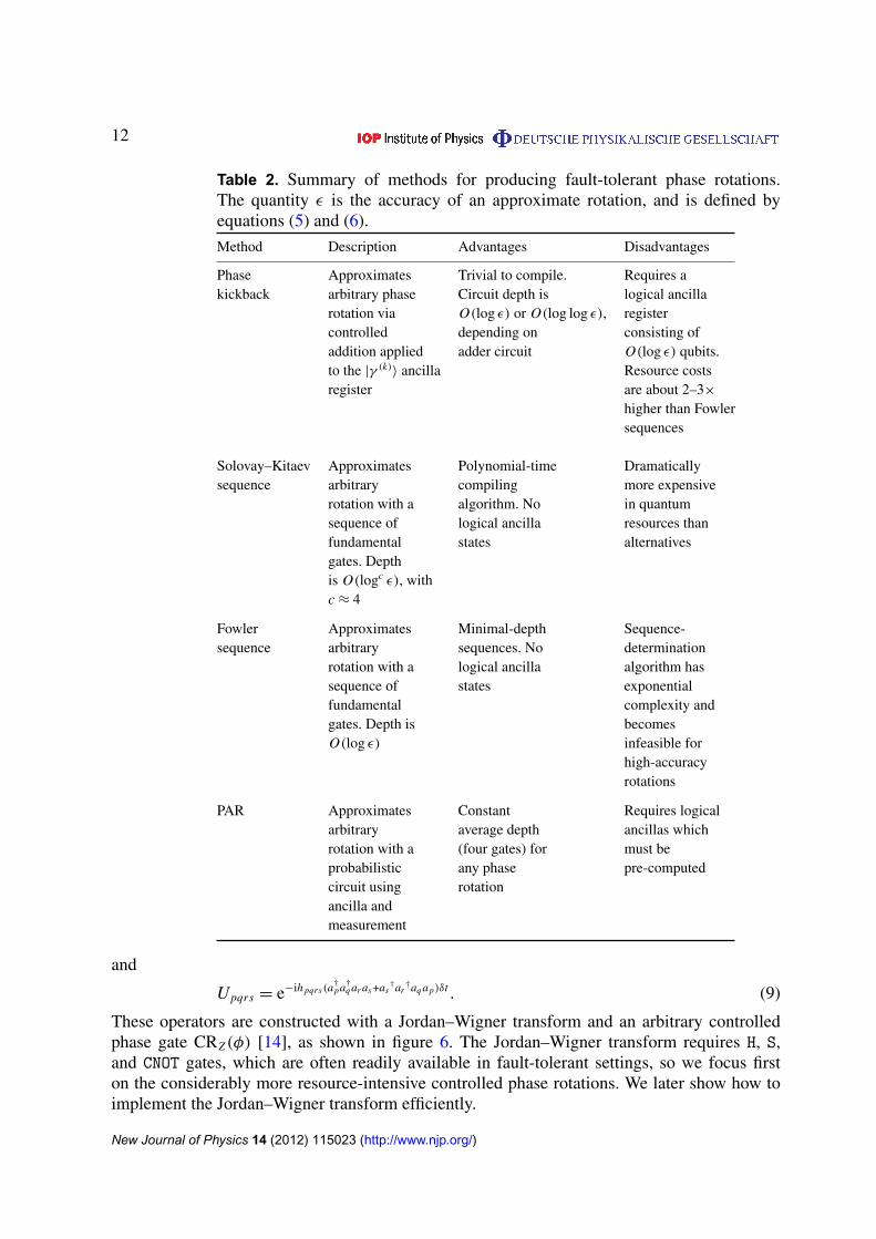
Table 2. Summary of methods for producing fault-tolerant phase rotations.The quantity ε is the accuracy of an approximate rotation, and is defined byequations (5) and (6).

Method Description Advantages Disadvantages

Phase Approximates Trivial to compile. Requires akickback arbitrary phase Circuit depth is logical ancilla

rotation via O(log ε) or O(log log ε), registercontrolled depending on consisting ofaddition applied adder circuit O(log ε) qubits.to the |γ (k)〉 ancilla Resource costsregister are about 2–3×

higher than Fowlersequences

Solovay–Kitaev Approximates Polynomial-time Dramaticallysequence arbitrary compiling more expensive

rotation with a algorithm. No in quantumsequence of logical ancilla resources thanfundamental states alternativesgates. Depthis O(logc ε), withc ≈ 4

Fowler Approximates Minimal-depth Sequence-sequence arbitrary sequences. No determination

rotation with a logical ancilla algorithm hassequence of states exponentialfundamental complexity andgates. Depth is becomesO(log ε) infeasible for

high-accuracyrotations

PAR Approximates Constant Requires logicalarbitrary average depth ancillas whichrotation with a (four gates) for must beprobabilistic any phase pre-computedcircuit using rotationancilla andmeasurement

and

Upqrs = e−ih pqrs(a†pa†

q ar as+as†ar

†aq ap)δt . (9)

These operators are constructed with a Jordan–Wigner transform and an arbitrary controlledphase gate CRZ(φ) [14], as shown in figure 6. The Jordan–Wigner transform requires H, S,and CNOT gates, which are often readily available in fault-tolerant settings, so we focus firston the considerably more resource-intensive controlled phase rotations. We later show how toimplement the Jordan–Wigner transform efficiently.

New Journal of Physics 14 (2012) 115023 (http://www.njp.org/)

13

H

H

( )ZR

H

H (- /2)XR

t

1

2 ( )ZR

(- /2)XR

( /2)XR

( /2)XR

Figure 6. Excitation operator e−ih12(a†1a2+a†

2a1)δt encoded into a quantumcircuit [14]. Above, θ = h12δt . The gate RX(−π/2)= H · S†

· H is available fromthe set in table 1. In this example, the control qubit |t〉 is used for phaseestimation, and the qubits |χ1〉 and |χ2〉 are basis functions (e.g. molecularorbitals). The controlled phase rotations CRZ(θ) must be approximated usingcircuits of available fault-tolerant gates.

3.1. Controlled phase rotations

As can be seen in figure 6, when Upq or Upqrs is implemented in a controlled operation (suchas in energy eigenvalue estimation, see also figure 1), the core component of the circuit is acontrolled phase rotation

CRZ(φ)=

1 0 0 00 1 0 00 0 1 00 0 0 eiφ

. (10)

One way to implement the controlled rotation in equation (10) is to deconstruct the operationinto CNOTs and single-qubit rotations [58], as shown in figure 7. Another method requires justone single-qubit rotation, as well as an ancilla |0〉, as shown in figure 8. Nielsen and Chuang[30] (p 182) provide a circuit decomposition for the Toffoli gate into gates in table 1. Weuse the circuit in figure 8 (requiring just one phase rotation) for the remainder of this paper,because the cost of one ancilla qubit is typically modest compared to a phase rotation. One canimplement phase kickback, gate approximation sequences, or PARs to produce the single-qubitrotations, as in section 2.4. Additionally, the PAR construction can be modified to producecontrolled rotations more directly. If the control qubit only controls other circuits betweenancilla production and the time a controlled-PAR is needed, as is the case for phase estimationalgorithms, one can create the ancillas (see figure 4) using controlled rotations with one of theabove methods and produce a controlled-PAR with the same cascading circuit.

The different methods of producing a controlled phase rotation are analyzed in figure 9. Wehave excluded Solovay–Kitaev sequences, which permits a linearly scaled vertical axis, showingthat each of these methods has execution time linear in log ε or constant. As before, the valuesfor Fowler sequences are extrapolated. We can see that Fowler sequences and phase kickbackare separated by approximately a factor of 3 in execution time, and the choice between the twowould be motivated by whether compiling the Fowler sequence is feasible or not. The PARcircuit requires one of the above methods to pre-compute ancillas.

3.2. Finite precision in pre-calculated integrals

The execution time of a second-quantized simulation algorithm is proportional to the number ofintegral terms h pq and h pqrs , as indicated by equations (7)–(9). We now consider how to speed up

New Journal of Physics 14 (2012) 115023 (http://www.njp.org/)

14

=(φ)ZR (φ/2)ZR

(φ/2)ZR

(-φ/2)ZR

Figure 7. Decomposition of a controlled phase rotation into CNOTs and fault-tolerant single-qubit rotations. If the control qubit only controls other circuits,as in phase estimation algorithms, the third phase rotation commutes with theCNOTs. In such an event, the third single-qubit rotations from all decompositionsof controlled rotations commute, and they can be combined into just onerotation prior to a non-commuting operation on this qubit (such as the QFTand measurement readout in figure 1). As a result, controlled rotations in phaseestimation algorithms are effectively decomposed into two CNOTs and twosingle-qubit rotations with this circuit.

=(φ)ZR

(φ)ZR

x

y

0

x

y

0

Figure 8. Controlled rotation CRZ(φ) (see equation (10)) between qubits |x〉 and|y〉 using two Toffoli gates, just one single-qubit rotation gate, and an ancilla |0〉.The ancilla qubit is conditionally set to |1〉 using a Toffoli gate, and a phase isimparted to this state with the rotation RZ(φ). A final Toffoli gate returns theancilla qubit to state |0〉.

the algorithm by omitting the integral terms that are negligibly small in magnitude. For a basisset consisting of M single-particle orbitals, the maximum number of integral terms is O(M4).In practice, however, the effort for evaluating these integrals often scales somewhere betweenO(M2) and O(M3) with modern implementations [59], because typically many integral termsmay be neglected for being smaller in magnitude than a cutoff threshold. Consequently, theexecution time of second-quantized simulation is determined by the number of pre-computedintegrals of the form h pq and h pqrs of sufficiently large magnitude, as well as the efficiencyof producing the corresponding arbitrary phase rotations in the quantum computer, such asCRZ(h pqδt) in the gate sequence for e−ih pq (a

†p(a)q +a†

q ap)δt [14].To illustrate how many integral terms are present in a typical chemical problem, we have

calculated the integrals for a second-quantized simulation of LiH. We performed calculationsin the minimal basis and in a triple-zeta basis, using the GAMESS quantum chemistry package[60, 61], at a bond distance of 1.63 Å, with an integral term cutoff of 10−10 in atomic units.We computed the number of integrals above cutoff using the STO-3G basis [62] containing12 spin orbitals (6 spatial orbitals) and the TZVP basis [63] containing 40 spin orbitals (20spatial orbitals). The cumulative number of integral terms as a function of cutoff in TZVP basisis plotted in figure 10. With the STO-3G basis, there were 231 non-zero molecular integrals,but only 99 of them were greater than 10−10 atomic units in magnitude. This is an order ofmagnitude below what is expected from O(M4) scaling. Considering the larger, more accuratebasis set (TZVP), there were 22 155 non-zero integrals, but only 10 315 were greater than the

New Journal of Physics 14 (2012) 115023 (http://www.njp.org/)

15

0.50

50

100

150

200

250

300

350

400

10-1

10-2

10-3

10-4

10-5

Circ

uit d

epth

(ga

tes)

Approximation error (ε)

Phase KickbackFowler SequencesPARs

Figure 9. Circuit depth for controlled phase rotations using various methods.A desired controlled rotation CRZ(φ) is approximated with a fault-tolerantcircuit Uapprox with accuracy ε = dist4(Uapprox,CRZ(φ)) using the method infigure 8. Solovay–Kitaev sequences are omitted here to permit comparison ofthe more efficient schemes on a linear scale. The bars on Fowler sequencedata indicate the standard deviation taken over 98 random-angle rotations. Thecontrolled-PARs have a depth of four gates, on average, regardless of rotationaccuracy. Phase kickback uses a ripple-carry adder since the addends have lessthan 16 bits [52]. If very high precision were desired, a carry-lookahead addercan achieve depth O(log log ε) at the expense of additional qubits and parallelcircuits (more T gates) [53].

cutoff. Figure 10 shows that a higher cutoff, such as 10−4, can further reduce the number ofintegrals in the TZVP basis implemented in the simulation. As a result, the effective number ofintegral terms the quantum computer must implement as phase rotations is nearly two ordersof magnitude less than the asymptotic analysis would suggest. This is an example of the over-estimation of the resource costs that can occur when using asymptotic estimates. This techniquebecomes particularly relevant in large molecules since distant particles interact weakly, and insuch an event, many of the associated integral terms may be negligibly small. Raising the cutoffthreshold impacts the accuracy of the simulation, so one must attempt to balance the resourcecosts of simulation with the usefulness of the result.

3.3. Jordan–Wigner transform using teleportation

The second-quantized algorithm uses Jordan–Wigner transforms to implement operators suchas e−ih pq (a

†paq +a†

q ap)δt , and this section shows how to perform such transforms in constant time. Aselaborated in [14], the circuits for Jordan–Wigner transforms often consist of ladders of CNOT

New Journal of Physics 14 (2012) 115023 (http://www.njp.org/)

16

10-7

10-6

10-5

10-4

10-3

10-2

10-1

100

101

0

2000

4000

6000

8000

10000

12000

Cutoff value (atomic units)

Num

ber

of in

tegr

als

Figure 10. The number of integral terms implemented in a second-quantizedsimulation of LiH using a TZVP basis, as a function of cutoff threshold. Onlyintegral terms with absolute value above the threshold are implemented incircuits, and the rest are neglected. As shown in the figure, a cutoff of 10−4

would require the algorithm to implement just over 9000 integral terms.

BSM

BSM

BSM

(a) (b) (c)

Figure 11. Rearrangement of the CNOT ladder common in Jordan–Wignertransforms using teleportation. (a) The original CNOT ladder requires anexecution time that grows with the extent of the simulation in qubits.(b) A conceptual diagram of what teleportation accomplishes. The qubits ‘move’backwards in time. (c) A valid quantum circuit that uses teleportation to movequbits in a manner which allows parallel computation of the CNOTs. The BSMis the Bell state measurement which teleports the qubits; the result of thismeasurement indicates the Pauli errors which are tracked by the Pauli frame [43].The Bell state |8+

〉 =1

√2(|00〉 + |11〉) can be prepared from |0〉 ancillas using

one H gate and one CNOT gate. Similarly, the BSM can be implemented using oneH, one CNOT, and measurement of the two qubits in the computational basis.

gates, such as the one in figure 11(a). In a simulation with M basis states, these ladders canextend across the entire register of qubits corresponding to these basis states, which leads to theO(M5) asymptotic runtime quoted in [19] when there are at most O(M4) integral terms.

New Journal of Physics 14 (2012) 115023 (http://www.njp.org/)

17

The CNOT ladder is a sparse network of Clifford gates, so we show how it may beimplemented in constant time using teleportation [34, 35]. Figure 11(b) gives an intuitive picturefor what will be accomplished. If the path of the qubits could be rearranged to somehowpropagate backwards in time, the CNOT gates could be implemented simultaneously. Qubitscannot move backwards in time per se, but they can be moved arbitrarily using teleportation;notice how the conceptual (but unphysical) circuit in figure 11(b) is realized by a physical circuitin figure 11(c). Ancilla Bell states |8+

〉 =1

√2(|00〉 + |11〉) are used to teleport qubits in this

rearranged CNOT ladder. Teleportation introduces a random Pauli error on the teleported qubit,but it is possible to track these errors and their propagation through CNOT gates using Pauliframes [43, 55, 56]. With this modification, it is possible to implement the Jordan–Wignertransform in constant time, which removes one of the bottlenecks to high-speed second-quantized simulation. This method could be adapted to implement other Clifford-group circuitsin constant time, at the expense of requiring enough ancilla Bell states.

3.4. Resource analysis for ground-state energy simulation of lithium hydride

Using the hypothetical quantum computer from section 2.4, we examine the resources requiredto perform simulation in second-quantized form. Estimates of the number of qubits requiredfor various instances of second-quantized chemical simulation have been reported previously[9, 19], so we focus instead on the execution time and effort to prepare fault-tolerant gates (herewe consider the number of T gates). Figure 12 shows both the circuit depth and the numberof T gates required to simulate LiH in the STO-3G basis as a function of rotation accuracythreshold εmax, for 1023 simulated time steps. The precision in the readout is proportional thenumber of time steps simulated. The energy estimate in this simulation has 10 bits of precision,and in general, 2n

− 1 steps are required for n bits of precision. If we assume that the durationof a single quantum gate is 1 ms (cf [43]), then the total execution time of the simulation rangesfrom ∼5.6 h using PARs to ∼3.8 years using Solovay–Kitaev rotations.

The number of T gates in figure 12 serves as an indication of the complexity demanded ofthe quantum computer. Although we do not delve into this matter, Jones et al [43] and Isailovicet al [54] discuss the importance (and difficulty) of producing these gates. What becomesapparent is that using PARs, while very fast, is also more expensive in the consumption ofT gates than directly implementing Fowler sequences or phase kickback. Choosing betweensuch approaches depends on the capabilities of the quantum computer, and we discuss thismatter in more detail in section 5.

To provide an indication of how much execution time in second-quantized simulationis devoted to phase rotations, figure 13 shows the relative ratio of circuit depth devotedto implementing rotations versus all other gates for each of the methods considered whensimulating LiH with rotation accuracy ε 6 10−4. It is clear here that Solovay–Kitaev has suchhigh circuit depth that it cannot be drawn to scale. We see also that Fowler and phase kickbacksequences require execution times that are comparable, whereas PARs actually do not representthe majority of the circuit depth, unlike all of the prior methods. This is an encouragingresult, because it shows that previous examinations that depended on Solovay–Kitaev sequencescan be improved by orders of magnitude with more efficient phase rotations [6]. We do notconsider Solovay–Kitaev sequences further in this investigation. The techniques for improving

New Journal of Physics 14 (2012) 115023 (http://www.njp.org/)

18

T g

ates

Approximation error (ε )max

10-1

10-2

10-3

10-4

10-5

Solovay−Kitaev SequencesPhase KickbackFowler SequencesPARs

107

108

109

1010

1011

107

108

109

1010

1011

1012

Cir

cuit

dept

h (g

ates

)

Figure 12. Total circuit depth and T gates for a second-quantized simulation ofLiH using the STO-3G basis, calculated for different constructions of controlledrotations as a function of accuracy εmax. For a given εmax, every controlledrotation CRZ(φ) in the algorithm is approximated with a fault-tolerant circuitUapprox with accuracy distance ε = dist4(Uapprox,CRZ(φ)) such that ε 6 εmax.An accuracy threshold εmax 6 10−4 is used in later analysis. This simulationimplements all integral terms in the Hamiltonian (see equation (7)). (Top) Circuitdepth using the gate set in table 1. In this plot, only the mean number ofgates for PAR circuits is shown. (Bottom) T gates required for each method.The controlled-PAR ancillas are produced using controlled rotations constructedusing Fowler sequences; six controlled-PAR ancillas are pre-computed for eachrotation, and only mean values are plotted. The sudden jump in Solovay–Kitaevresource costs is because many controlled rotations in this algorithm have a smallangle φ ≈ 0 that is approximated with identity gate at low precision, whereas theother methods are using a typical sequence length for arbitrary φ.

New Journal of Physics 14 (2012) 115023 (http://www.njp.org/)

19

1

1

1

1

7460

7.0

(0.24)

Clifford Gates Approximate Phase Rotations

Solovay-Kitaev:

Fowler Sequences:

PAR (in-place):

1 20.0Phase Kickback:

Figure 13. The relative amount of time (circuit depth) of a fault-tolerant,second-quantized simulation of LiH devoted to Clifford gates {X,Y,Z,H,S,CNOT}versus phase rotations that must be approximated. In this example, rotationsare computed to an accuracy ε 6 10−4. The relative circuit depth of rotationscalculated by the Solovay–Kitaev algorithm is too large to be drawn to scalehere. In the case of PAR, the ancillas must be pre-computed with a method suchas Fowler sequences, but this can be carried out in parallel with other algorithmoperations.

Table 3. Summary of methods for efficient second-quantized chemicalsimulation. The quantity M is the number of basis functions used in therepresentation of the chemical problem; larger basis sets produce more accurateresults at the expense of greater circuit complexity.

Method Description Advantages Disadvantages

Finite-precision Neglect to implement Second-quantized None if the cutoffcutoff in integral terms circuit complexity is threshold issecond-quantized below a chosen reduced in both below gateintegrals cutoff in the depth and approximation

algorithm execution the number of T gates accuracy

Jordan–Wigner Use a Second-quantized Teleportationtransform using teleportation circuit depth circuit requiresteleportation circuit to reduces to at at most 3M − 4

implement most O(M4) qubits instead ofJordan–Wigner from O(M5) M (only duringtransform in Jordan–Wignerconstant time transform)

second-quantized simulation are summarized in table 3. The methods for determining resourcecosts are summarized in appendix A.

4. Simulating chemical structure and dynamics in first-quantized representation

The first-quantized simulation algorithm is in some ways more complex than the second-quantized algorithm, but for problems in chemistry larger than a handful of particles, it iscomputationally faster. A first-quantized simulation is essentially a finite-difference method forsolving the Schrodinger equation. Configuration space is discretized into a Cartesian grid, andeach particle (e.g. electron) has a wavefunction expressed in a quantum register that encodes a

New Journal of Physics 14 (2012) 115023 (http://www.njp.org/)

20

probability amplitude at each coordinate on the grid. For example, let us imagine that we forma position-basis representation for a single electron on a 2p

× 2p× 2p grid, which requires only

3p qubits. Explicitly, the electronic wavefunction is represented as

|ψe〉 =

2p−1∑

x,y,z=0

c(x, y, z) |x〉 |y〉 |z〉 =

∑r

c(r) |r〉 , (11)

where c(x, y, z) is the complex probability amplitude for the electron to occupy the volumeelement centered at the position r ≡ (x, y, z). The rightmost part of equation (11) is shorthandthat will be used throughout this section. The spin degree of freedom can easily be incorporatedby including an extra qubit, and to describe a many-electron state, the wavefunction has to beproperly anti-symmetrized [37, 64].

To simulate the evolution of a time-independent molecular Hamiltonian H for problemsin quantum chemistry, we adopt the method given in [3, 20]. The complete Hamiltonian infirst-quantized form can be expressed as the sum of the kinetic (T ) and potential (V ) operators

H= T + V = −

∑i

h2∇

2i

2mi+

1

2

∑i 6= j

qiq j

4πε0ri j, (12)

where the indices i and j run over all particles (electrons and nuclei) of any given molecule.Here ri j ≡

∣∣ri − r j

∣∣ is the distance between particles i and j , which carry charges qi and q j

respectively.Let us outline how first-quantized simulation works before delving into details. The core

of the algorithm is evolving the Hamiltonian in simulated time, achieved by applying thepropagator U(t)= exp(−iHt) (setting h = 1 and assuming H is time-independent), which solvesthe time-dependent Schrodinger equation [2]. This process is readily achieved using the splitoperator approximation, a form of Trotter–Suzuki decomposition [19, 27, 65, 66], where thekinetic and potential energy operators are simulated in alternating steps as

U(t)= e−iHt≈

[e−iT δt/2e−iV δte−iT δt/2

] tδt. (13)

The exponent tδt is the number of times the circuit corresponding to the expression in brackets

is implemented, so it is always an integer. The operators e−iV δt and e−iT δt are diagonal inthe position and momentum bases, respectively. One can switch the encoded configurationspace representation between these two bases by applying the QFT to each spatial dimensionof the wavefunction (cf equation (11)), which can be efficiently implemented in a quantumcomputer [48]. Kassal et al [20] show how to construct quantum circuits for operators e−iV δt

and e−iT δt , and in this section, we complement that work with analysis of fault-tolerant versionsof these operators.

To make an algorithm fault-tolerant, its constituent operations must be decomposed intocircuits of fault-tolerant primitive gates such as those in table 1. Consider the potential energypropagator e−iV δt as an example. Given a b-particle wavefunction in the position basis as∣∣ψ1,2,...,b

⟩=

∑r1,r2,...,rb

c(r1, r2, . . . , rb) |r1r2 . . . rb〉 , (14)

where c(·) is the complex amplitude as a function of position in configuration space andsubscripts correspond to particles in the system, one calculates the phase evolution of the

New Journal of Physics 14 (2012) 115023 (http://www.njp.org/)

21

potential operator e−iV δt in three steps, as follows:∑r1,...,rb

c(r1, . . . , rb) |r1 . . . rb〉 |000 . . .〉

−→

∑r1,...,rb

c(r1, . . . , rb) |r1 . . . rb〉 |V (r1, . . . , rb)〉 (15)

−→

∑r1,...,rb

e−iV (r1,...,rb)δtc(r1, . . . , rb) |r1 . . . rb〉 |V (r1, . . . , rb)〉 (16)

−→

∑r1,...,rb

e−iV (r1,...,rb)δtc(r1, . . . , rb) |r1 . . . rb〉 |000 . . .〉 . (17)

Firstly, equation (15) calculates the potential energy as a function of position coordinates [20](note that V is diagonal in this basis) and stores the result in a quantum register|V (r1, r2, . . . , rb)〉 to some finite precision. Appendix C describes how to implementthis quantum circuit for molecular Hamiltonians. Secondly, equation (16) uses the|V (r1, r2, . . . , rb)〉 register in a ‘quantum variable’ phase rotation that imparts a phase toeach grid point of the wavefunction in position basis proportional to the potential energy atthose coordinates. This section discusses how to implement the quantum variable rotation(QVR) using fault-tolerant quantum circuits. Finally, the quantum circuit from the first stepis reversed in equation (17) to reset the |V (r1, r2, . . . , rb)〉 register to |000 . . .〉, also known as‘uncomputation’ [30]. The sequence of these three steps is equivalent to the operation e−iV δt |ψ〉.

The kinetic energy propagator e−iT δt is calculated similarly in three steps, with thesecond also being a QVR. This operator is diagonal in momentum basis, so we transform therepresentation of the system wavefunction from position basis {x, y, z} to momentum basis{kx , ky, kz} by applying a QFT along each spatial dimension of the encoding in equation (11).This form permits efficient calculation of the kinetic energy operator [20], which is described inappendix C.

4.1. Quantum variable rotation

The phase rotation subroutine in the first-quantized simulation algorithm imparts a quantumphase to each binary-encoded phase state in a superposition |θ〉 =

∑j c j

∣∣φ j

⟩stored in a

quantum register (c j ’s are arbitrary complex amplitudes). Formally, it is the transformation∑j

c j |φ j〉 −→

∑j

e2π iξφ j c j |φ j〉, (18)

which generalizes the operation in equation (16) using ξ , which is a scaling factor that varieswith implementation, as explained below and in appendix C. Each 06 φ j < 1 is a finitebinary representation of a rotation on the unit circle encoded in a quantum register (the angle,in radians, divided by 2π ). Equation (18) is the QVR, which is essential to first-quantizedsimulation. We show how to implement this phase rotation subroutine using phase rotationsfrom previous sections, as well as a new construction based on phase kickback. At the end ofthe section, we analyze the resource costs of these methods.

To produce a QVR, various circuit manipulations are possible. The first is to simply applya single-qubit rotation to each qubit in register |θ〉, as shown in figure 14. Each individualrotation could be created using the techniques in section 2. Since a t-bit QVR requires t

New Journal of Physics 14 (2012) 115023 (http://www.njp.org/)

22

q-1

q-2

q-3

q-4

(2 /2)ZR

(2 /4)ZR

(2 /8)ZR

(2 /16)ZR

. . .

Figure 14. QVR decomposed into single-qubit rotations applied to each qubitin the |θ〉 register consisting of q qubits (see equation (18)). |θq−1〉 refers to themost significant bit in the register |θ〉, etc.

separate bitwise rotations, we require that each rotation has accuracy ε/t to achieve accuracyε in the QVR, where we have used the fact that the distance measure in equation (5) obeysthe triangle inequality [33]. If the QVR is controlled by another qubit (e.g. if the propagator iscontrolled by a ‘simulated time’ qubit as in figure 1), then the gates in figure 14 are replaced withcontrolled rotations from section 3.1. In either case, one must know the quantity ξ in advance tocompile these gates; typically, ξ is a product of physical constants and simulation parameters,as explained in appendix C.

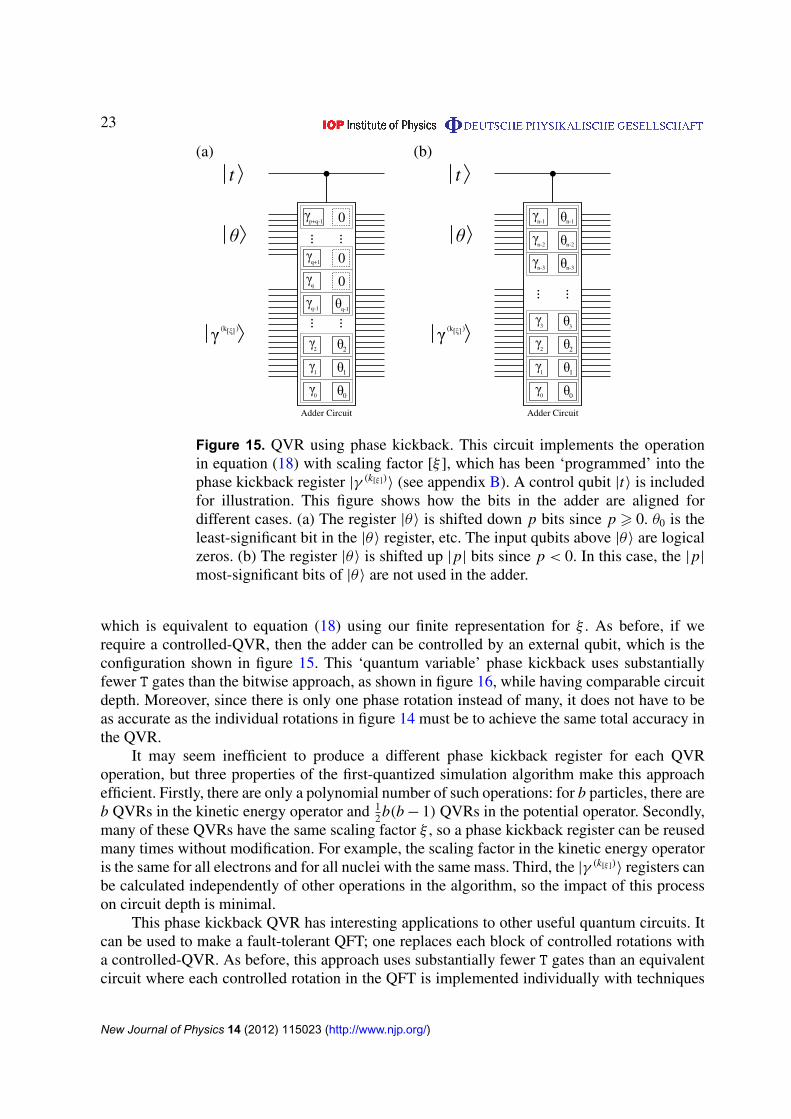
The QVR can also be produced in a more elegant manner using phase kickback. Rather thanapplying bitwise gates to the |θ〉 register, we instead use the entire register in a modified versionof the phase kickback procedure. Firstly, we require a binary approximation to ξ , denoted[ξ ]. Secondly, we define some quantities that describe this quantum circuit. Let m denote thenumber of significant bits in [ξ ], minus the number of trailing zeros. Define w = blog2[ξ ]c,or in other words, w is the largest integer such that 2w 6 [ξ ]. Denote p = (m − 1)−w, whichis how many bits we must shift [ξ ] up to produce an odd integer (if p < 0, we shift down).Following equation (18) and the preceding text, let q be the number of qubits in |θ〉. Defineintegers k[ξ ] = (2p)[ξ ] and uφ = (2q)φ for some arbitrary φ ∈ [0, 1) represented using q bits.Thirdly, we construct a phase kickback ancilla register |γ (k[ξ ])〉 of size n = p + q qubits, usingtechniques in appendix B. Finally, we perform phase kickback with an addition circuit betweenregisters |θ〉 and |γ (k[ξ ])〉 (in-place addition applied to |γ (k[ξ ])〉), except this time the |θ〉 registeris shifted in one of two ways, as shown in figure 15. If p > 0, then the |θ〉 register is shifteddown by p qubits, and the |θ〉 register is padded with p logical zeros at the most-significant sideof the adder input (figure 15(a)). If p < 0, then |θ〉 is shifted up by |p| qubits, so that the |p|

most-significant bits of |θ〉 are not used in the adder (figure 15(b)). If n 6 0, then all rotationsare identity and no QVR circuit is constructed.

We now confirm that this procedure produces the intended QVR. Using equation (3), wesee that the above procedure will implement a phase rotation of∑

j

c j

∣∣φ j

⟩−→

∑j

e2π ik[ξ ]uφ j /2p+q

c j

∣∣φ j

⟩. (19)

Since k[ξ ] = (2p)[ξ ] and uφ = (2q)φ, this is the same as∑j

c j

∣∣φ j

⟩−→

∑j

e2π i[ξ ]φ j c j

∣∣φ j

⟩, (20)

New Journal of Physics 14 (2012) 115023 (http://www.njp.org/)

23

p+q-1

q+1

q

q-1

2

0

q-1

1

0

2

1

0

0

0

Adder Circuit

[ ](k )

t t

n-1

n-2

n-3

3

2

3

1

0

2

1

0

Adder Circuit

[ ](k )

n-3

n-2

n-1

(a) (b)

Figure 15. QVR using phase kickback. This circuit implements the operationin equation (18) with scaling factor [ξ ], which has been ‘programmed’ into thephase kickback register |γ (k[ξ ])〉 (see appendix B). A control qubit |t〉 is includedfor illustration. This figure shows how the bits in the adder are aligned fordifferent cases. (a) The register |θ〉 is shifted down p bits since p > 0. θ0 is theleast-significant bit in the |θ〉 register, etc. The input qubits above |θ〉 are logicalzeros. (b) The register |θ〉 is shifted up |p| bits since p < 0. In this case, the |p|

most-significant bits of |θ〉 are not used in the adder.

which is equivalent to equation (18) using our finite representation for ξ . As before, if werequire a controlled-QVR, then the adder can be controlled by an external qubit, which is theconfiguration shown in figure 15. This ‘quantum variable’ phase kickback uses substantiallyfewer T gates than the bitwise approach, as shown in figure 16, while having comparable circuitdepth. Moreover, since there is only one phase rotation instead of many, it does not have to beas accurate as the individual rotations in figure 14 must be to achieve the same total accuracy inthe QVR.

It may seem inefficient to produce a different phase kickback register for each QVRoperation, but three properties of the first-quantized simulation algorithm make this approachefficient. Firstly, there are only a polynomial number of such operations: for b particles, there areb QVRs in the kinetic energy operator and 1

2b(b − 1) QVRs in the potential operator. Secondly,many of these QVRs have the same scaling factor ξ , so a phase kickback register can be reusedmany times without modification. For example, the scaling factor in the kinetic energy operatoris the same for all electrons and for all nuclei with the same mass. Third, the |γ (k[ξ ])〉 registers canbe calculated independently of other operations in the algorithm, so the impact of this processon circuit depth is minimal.

This phase kickback QVR has interesting applications to other useful quantum circuits. Itcan be used to make a fault-tolerant QFT; one replaces each block of controlled rotations witha controlled-QVR. As before, this approach uses substantially fewer T gates than an equivalentcircuit where each controlled rotation in the QFT is implemented individually with techniques

New Journal of Physics 14 (2012) 115023 (http://www.njp.org/)

24

102

103

104

T g

ates

10−6

10−5

10−4

10−3

10−2

10−1

Approximation error (ε)

PAR (Single−Qubit Bitwise)Phase Kickback (Single−Qubit Bitwise)Fowler (Single−Qubit Bitwise)Phase Kickback (Quantum Variable)

Figure 16. Number of T gates required to produce a QVR with various methods,assuming ξ = 1 and number of significant figures is chosen to satisfy theapproximation error ε. The special-purpose ‘quantum variable’ phase kickbackclearly requires the least circuit effort, and the asymptotic scaling of T gates islinear in log ε for this approach and super-quadratic for the others. The circuitdepth for Fowler or phase kickback approaches is equivalent to the comparablesingle-qubit rotation; however, the PAR must succeed across all individualrotations for this circuit to succeed, so the mean circuit depth increases slightly.In the above, ten rounds of PAR ancilla are pre-computed for each single-qubitrotation in the QVR.

in section 3.1, and the same methods can be applied to an approximate QFT [67] by simplytruncating the size of the |γ (1)〉 register. The phase kickback QVR can also be used to efficientlyproduce ancillas for PAR if the particular rotation RZ(φ) is required frequently, which can haveapplications to second-quantized simulation. If we denote the state |+〉 =

1√

2(|0〉 + |1〉), then an

input state of |+〉 |+〉 |+〉 . . . will be transformed using QVR (with appropriate ξ ) into the set ofancillas for PAR, but requiring only one addition circuit for the entire set instead of a phasekickback addition or Fowler sequence for each ancilla qubit, which can be seen by comparingfigure 14 with the ancilla preparation in figure 4. Creating the necessary |γ (k[ξ ])〉 for this processis costly, so there is a net gain only if a certain rotation angle φ is required often.

4.2. Improved parallelism in potential energy operator

The majority of the circuit effort in first-quantized simulation is devoted to calculating thepotential energy [20]. We introduce here a technique to substantially speed up the calculationof the potential energy operator V , which is simply the sum of the Coulomb interactionsVi j =

qi q j

4πε0ri jbetween all pairwise combinations of the electrons and nuclei. Note that this

operator is a function of the positions ri of the system particles only, so it is diagonal in the

New Journal of Physics 14 (2012) 115023 (http://www.njp.org/)

25

position basis |r1r2 . . . rb〉. This fact means that all terms Vi j commute with each other, so theymay be calculated in any order. Moreover, there are many sets of the Vi j operators that aredisjoint, which means that each particle in the system is acted on by just one operator in the set.Using this observation, for example, we may calculate the Coulomb interaction V12 betweenparticles 1 and 2 at the same time as V34 between particles 3 and 4, and so on. In general, for asystem of b particles, there are 1

2b(b − 1) pairwise interactions, and we can perform bb2c pairs

in parallel, which means that a potential energy operator with O(b2) terms can be calculated inO(b) time. This parallelism can increase the speed of simulation significantly since evaluationof the potential energy dominates resource costs [43].

The potential operator calculation can be further parallelized to achieve O(log b) or O(1)(constant) circuit depth. Exploiting the fact that all Vi j are diagonal in position basis (andhence commute), we use transversal CNOT gates to copy the data in the position-basis particlewavefunction onto multiple empty quantum registers. For a single particle, this process is 2p

−1∑x,y,z=0

c(x, y, z) |x〉 |y〉 |z〉

|000 . . .〉 |000 . . .〉 . . .

→

2p−1∑

x,y,z=0

c(x, y, z) (|x〉 |y〉 |z〉) (|x〉 |y〉 |z〉) (|x〉 |y〉 |z〉) . . . . (21)

For b particles, the copy operation is performed b − 2 times (for b − 1 total copies), which canbe fanned out using a binary tree with depth dlog2(b − 1)e; constant depth can be achieved insome quantum computer architectures which support one-control/many-target CNOTs [43, 57]or in general architectures using a teleportation circuit similar to those described in section 3.3.This approach is similar to that employed in [47] to produce a parallel circuit for the QFT. Thesystem wavefunction is now expanded to the state∣∣ψexpand

⟩=

∑r1,...,rb

c(r1, . . . , rb) (|r1〉)⊗(b−1) . . . (|rb〉)

⊗(b−1) , (22)

which requires O(b2) memory space. Note that this process is not cloning—the position-basis particle registers are still entangled to one another. With multiple accessible copies ofeach particle’s position-basis information, the particles are matched in all b(b − 1) possiblepairings, and the potential energy operator applied to each pairing in parallel, which can beaccomplished in constant time, but still requires O(b2) circuit effort. After each of the potentialenergy operators Vi j kicks back a phase, the excess copies of each particle wavefunction areuncomputed by reversing the tree of CNOTs above. The preceding example demonstrates that itis possible to calculate V in time which is sub-linear in the number of particles, even if eachVi j is treated as a black box operator. In practice, more efficient circuits can be produced bygenerating the internal ‘workspace’ registers of V in parallel, rather than making copies of theinput registers

∑r1,...,rb

c(r1, . . . , rb) |r1 . . . rb〉 (see appendix C).

4.3. Resource analysis for first-quantized molecular simulations

The advantage of using the first-quantized approach is that the approximation errors of thesimulation are systematically improvable by increasing the spatial precision of the wavefunction

New Journal of Physics 14 (2012) 115023 (http://www.njp.org/)

26

2 4 6 8 10 12 14 16 18 200

0.2

0.4

0.6

0.8

1

1.2

1.4

1.6

1.8

2x 10

9

Number of particles

Cir

cuit

dept

h (g

ates

)

In-place potential calculationsFully-parallel potential calculations

Figure 17. Circuit depth for two instances of first-quantized simulation. Thein-place calculation of potential energy computes each pairwise Coulombinteraction in sets of non-overlapping particle pairs, and both the depth andnumber of qubits required increase linearly with the number of particles. Thefully parallel calculation creates many copies of the wavefunction to permit thepotential energy to be determined in constant time, at the expense of requiringsubstantially more application qubits (quadratic in the number of particles). Inboth cases, the wavefunction precision along any spatial dimension is ten qubits,and the simulation uses 1023 time steps for 10 bits of precision, or ∼3 significantfigures.

and the temporal precision of the time steps. However, calculating kinetic and potential energyinteractions requires quantum arithmetic circuits and phase rotations, which together requiresubstantial resources in terms of fault-tolerant gates and qubits. Figure 17 shows two versionsof first-quantized simulation using the techniques for parallel calculation of potential energyfrom the previous section. Although constant-depth evaluation of the Hamiltonian is possible,it requires a significantly larger quantum computer to achieve the parallel calculations, so thisimplementation is probably best suited to large-scale quantum computers.

Examining figure 17, note that the circuit depth at six particles (e.g. LiH) is comparableto that of the equivalent PAR-based second-quantized simulation in figure 12 while requiringmany more qubits, indicating that first-quantized simulation is more appropriate for largermolecules than LiH, since the circuit depth for first-quantized simulation is asymptotically lessthan second-quantized as particle number is increased [19]. Moreover, these calculations haveassumed that the spatial precision is ten qubits for any molecules with 2–20 particles. As the sizeof the molecule increases, the number of qubits for each dimension of the encoded wavefunctionwill have to increase as the molecule itself is spatially larger. One may also choose to increasespatial resolution to achieve a higher-precision simulation. Each of the methods we propose forimproving first-quantized simulation are summarized in table 4. Appendix A explains how theresources were calculated.

New Journal of Physics 14 (2012) 115023 (http://www.njp.org/)

27

Table 4. Summary of methods for efficient first-quantized chemical simulation.The quantity b is the number of particles in the chemical problem, whichinfluences algorithm resource costs.

Method Description Advantages Disadvantages

QVR Use phase Reduces Not the minimalkickback to apply a complexity of depth achievable,fault-tolerant first-quantized such as with PARsphase rotation simulation.to each element Circuit depth isin a superposition, essentially theproportional same as single-qubitto the binary-encoded phase kickback,value of that element but the QVR

requires substantiallyfewer T gatesthan the methodin figure 14

Parallel Reduce potential Shorter circuit Concurrentevaluation operator circuit depth than computationof potential depth using calculating all requires more T gatesenergy terms parallel computation 1

2 b(b − 1) terms simultaneouslyindividually

Teleportation Use a Potential Circuit size incircuit expansion teleportation operator can be qubits increasesfor potential operator circuit to evaluated in a to O(b2) from O(b)

‘control-copy’ time which isposition-basis independent ofwavefunction in problem sizeconstant time

5. Comparing simulation methods

The prior sections illustrate that there exist numerous ways to simulate a molecular Hamiltonian,including choices between encoded representation in a quantum computer and the way fault-tolerant rotations are prepared. The final result one desires to know is, which method is best?Determining an optimal approach is subjective to the quantum computing resources available,so in this section we describe how to make such a decision.

To visually compare different implementations of a simulation algorithm, we plot theefficient frontier for each method in a plane defined by machine size (qubits) on the x-axisand execution time (circuit depth) on the y-axis. The efficient frontier is the set of all points(size, depth) such that for each achievable machine size, the (achievable) depth is minimized,and vice versa. As an example, figure 18 shows the efficient frontiers of various implementationsof a LiH simulation.

New Journal of Physics 14 (2012) 115023 (http://www.njp.org/)

28

101

102

103

107

108

109

1010

1011

1012

Second-Quantized(Solovay-Kitaev)

Second-Quantized(Phase-Kickback)

Second-Quantized(Fowler)

Second-Quantized(PAR)

First-Quantized(Phase-Kickback QVR)

Quantum computer size (application qubits)

Alg

orith

m r

untim

e (c

ircu

it de

pth

in g

ates

)

Figure 18. The efficient frontiers for various implementations of simulating LiHground state energy on a quantum computer. Each star data point corresponds tothe equivalent method in figure 12, at rotation accuracy εmax 6 10−4; similarly,first-quantized simulations use QVRs with the same accuracy. The PAR frontier(purple) and first-quantized frontier (brown) have adjustable parameters thatreduce circuit depth through parallel computation at the expense of increasedsystem size (application qubits). For example, the PAR-based algorithm onlyachieves the circuit depth shown in figure 12 when the system has 68 qubits,which is the yellow star here.

To determine the optimal implementation, one specifies a cost function g(x, y), whichassociates with any point (x, y) a ‘cost’ to implement simulation using these parameters. Forexample, cost could be the estimated engineering challenge to produce a quantum computer ofsize x qubits combined with a penalty for the execution time of y gates, which is a measure ofperformance. Minimizing the cost function along each efficient frontier gives the optimal set ofparameters for that particular method, and minimizing over all efficient frontiers gives the bestimplementation that is known to be achievable.

For the various implementations for a LiH simulation in figure 18, it seems likely that onewould choose between the compact algorithm with Fowler gate sequences or the faster versionwith PAR sequences, which requires additional qubits to compute the necessary ancillas. First-quantized can potentially deliver the fastest execution time here, but for this problem the numberof qubits required is substantially greater. Still, first-quantized gains an appreciable performanceadvantage if the number of particles is increased or if one moves to simulating time-varyingdynamics [19].

Naturally, future algorithm advancements could produce new frontiers that are moredesirable for a given cost function. In general, one would like to make such comparisons,which can inform design decisions for quantum hardware, with full consideration of the costto implement error correction, produce non-Clifford group gates (e.g. T gates), and so forth.Future work building on this investigation and prior efforts, such as [6, 43, 54, 68], shouldinclude such comprehensive system analysis.

New Journal of Physics 14 (2012) 115023 (http://www.njp.org/)

29

6. Conclusions

This paper examines the methods required to simulate chemistry on a fault-tolerant quantumcomputer. A crucial operation in these algorithms is the production of phase rotations, andseveral approaches—phase kickback, gate approximation sequences, PARs, and QVRs—areanalyzed. First, it should be clear that sequences generated by the Solovay–Kitaev algorithmare not nearly as efficient as the alternatives, phase kickback and Fowler sequences. Fowlersequences are the shortest for a fault-tolerant single-qubit rotation, but the classical computingeffort required to determine such sequences becomes intractable for high-precision (e.g.ε < 10−6) rotations. Recently, Bocharov and Svore have presented an alternative algorithmfor finding depth-optimal gate sequences which might feasibly provide high-precisionrotations [69]. Phase kickback is a versatile technique that produces rotations comparableto Fowler’s algorithm in resource usage, with the former having circuit depth O(log ε) orO(log log ε) gates and requiring O(log ε) T gates. Furthermore, the underlying circuit forphase kickback is an adder, which can be determined using efficient classical algorithms(unlike Fowler’s algorithm), and phase kickback can be extended more readily to QVRs. ThePAR allows the quantum algorithm to achieve exceptionally low-circuit-depth rotations, at theexpense of computing ancillas in advance (which is less efficient in terms of T gates). Finally,the QVR is particularly useful for first-quantized simulation. The relative merits of the methodsfor producing phase rotations are compared in table 2.

This investigation also examined two variants of the simulation algorithm, second-quantized and first-quantized, whose primary difference is the way wavefunctions are encodedand operated upon. Generally speaking, second-quantized is a more compact representation,requiring fewer qubits, but it requires asymptotically longer execution times than first-quantized, measured in circuit depth, as the problem size increases in terms of independentparticles to simulate. Our results provide a more nuanced way to compare these methodsby explicitly considering the possible ways to make the algorithms compatible with fault-tolerant quantum computing and the resulting resource costs incurred. We have also introducedseveral improvements to the simulation algorithms. In the second-quantized approach, one canneglect some of the integral terms smaller in magnitude than a cutoff threshold, implementthe Jordan–Wigner transform in constant time, and use PARs to substantially reduce circuitdepth, at the expense of requiring parallel production of the pre-computed PAR ancillas. Infirst-quantized, we demonstrated how to produce QVRs with arbitrary scaling factor, as well ashow to parallelize the calculation of the potential energy to time linear in system size (withoutincrease in qubits) or to constant time (requiring a number of qubits that grows quadraticallyinstead of linearly with the number of particles simulated). The methods we present for efficientchemical simulation on quantum computers are summarized in tables 3 and 4.

Although we have focused on simulating quantum chemistry, these methods can beextended to simulating other Hamiltonians on quantum computers, such as spin latticemodels [4], lattice gas automata [70] and lattice gauge theories [71], or quantum chaostheories [72]. Moreover, the fault-tolerant rotations could find application in other quantumalgorithms, including any which require a Fourier transform. This investigation provides aflexible set of methods for making simulation algorithms practically realizable on fault-tolerantquantum computers.

New Journal of Physics 14 (2012) 115023 (http://www.njp.org/)

30

Acknowledgments

The authors would like to thank Kevin Obenland for suggesting improvements to quantumcircuits; Paul Pham for providing assistance with Solovay–Kitaev code; Aram Harrow andIsaac Chuang for helpful discussions on Solovay–Kitaev; and Austin Fowler for providingcode for minimum-length approximation sequences. This work was supported by the NationalScience Foundation CCF-0829694, the University of Tokyo Special Coordination Funds forPromoting Science and Technology, NICT, and the Japan Society for the Promotion ofScience (JSPS) through its ‘Funding Program for World-Leading Innovative R&D on Scienceand Technology (FIRST Program).’ NCJ was supported by the National Science FoundationGraduate Fellowship. JDW acknowledges support from National Science Foundation awardnumber 1017244. MHY and AAG acknowledge support from the Air Force Office of ScientificResearch, award number FA8721-05-C-0002. AAG acknowledges support from the Alfred PSloan Foundation, and the Camille and Henry Dreyfus Foundation.

Appendix A. Methods for calculating resources

We briefly describe how the resources for quantum circuits were calculated. Beginning withsingle-qubit phase rotations, the Solovay–Kitaev algorithm is described in [32], while theFowler algorithm is described in [33]. Gate sequences for rotations were generated using thesealgorithms, and the total circuit depth and number of T gates were recorded. Phase kickbackimplements an adder circuit, and we select the CDKM adder (named for the authors of [52]).For reference, an n-qubit addition for phase kickback requires the n-qubit ancilla state |γ (k)〉

and n ancilla qubits. The latter ancilla qubits (representing an input to the adder) are initializedto the binary representation of the rotation angle, conditioned on the qubit to which the rotationis applied, which is accomplished using 2n CNOT gates that can be implemented in constanttime using the methods in section 3.3. The depth of the adder is 2n − 3 Toffoli gates and 5CNOT gates. Our implementation of the Toffoli gate uses 11 time steps, but recent work showsmany variations are possible [69]. The depth of our n-bit adder-based phase-kickback rotationis 22n − 26, which includes the parallel CNOT gates for setting the ancilla addend. Each Toffoligate requires 7 T gates, so the CDKM adder has 14n − 21 T gates in total.

Controlled phase rotations are built using single-qubit rotations. The Fowler and Solovay–Kitaev sequences require effectively two single-qubit rotations (see section 3.1); the rotationsare inverses of each other, so the circuits for the two rotations are mirror images, and thetotal resources (depth and T gates) are doubled. Phase kickback requires only the slightestmodification to become a controlled rotation. The n ancilla states are initialized to rotation angleconditioned on both the control and target qubit for this rotation. This requires two Toffolis (oneat the start and one at the end) and 2n − 2 additional CNOT gates (which can be implemented in aparallel fashion). The second-quantized algorithm is implemented using the methods describedin [14] and each of these types for controlled rotations. The depth and T gates are given by thenumber of integral terms times the controlled phase rotation resource requirements, plus circuitsfor each of the necessary Jordan–Wigner transforms.

The first-quantized simulation algorithm is implemented using arithmetic circuits andQFTs. Resource analysis for exact and approximate QFTs is given in [30, 47, 48]. Detailedexplanation of the arithmetic operations for this algorithm is given in [20] and appendix C.Each arithmetic circuit is decomposed into CDKM adders. The phase rotations in the kinetic

New Journal of Physics 14 (2012) 115023 (http://www.njp.org/)

31

operators, potential operators, and QFT are implemented using phase-kickback QVRs, each ofwhich requires a single CDKM adder.

Appendix B. Transforming the phase kickback register

In some situations it is useful to change the k-value in |γ (k)〉, the phase kickback ancilla register(see equation (2)). Without control over k, the QVR in section 4.1 would require solvingequation (4) in a quantum circuit; this step would in turn require a multiplication operation,which can be expensive in terms of quantum gates. We deviate here from [46] and proposea simple way to avoid the expensive operations associated with modular multiplication. Thespecific ancilla state |γ (1)〉 does not require an additional circuit to solve equation (4), so wecreate this state explicitly using a simple transform |γ (k)〉 → |γ (1)〉. We begin by factoring the|γ (k)〉 register into individual qubits (note that all such states are separable, i.e. not entangled):

|γ (k)〉 =1

√N

N−1∑y=0

e−2π iky/N|y〉

=1

√N

(|0〉 + e−2π ik/2

|1〉)⊗

(|0〉 + e−2π ik/4

|1〉)⊗ · · ·

⊗(|0〉 + e−2π ik/2n

|1〉). (B.1)

We convert this state into |γ (1)〉 with a series of single-qubit phase rotations using the controlledaddition circuit from figure 2. Since k is odd, the first bit of our ancilla register is always

1√

2(|0〉 − |1〉). The next bit must be rotated by the phase gate RZ(π(k − 1)), which is either

identity or Z, depending on k. In general, the corrective gate applied to the mth bit is the phaserotation RZ(2π k−1

2m−1 ), which may be produced using the preceding m − 1 bits of the ancillaregister and phase kickback. By iterating through all qubits in the register, we complete thetransformation with circuit depth O(n2) gates or less, depending on the type of adder used inphase kickback. This procedure can be generalized to any transformation |γ (k)〉 → |γ (l)〉 for oddintegers 16 k, l < 2n, where n is the number of bits in the phase kickback register.

Appendix C. Quantum circuits for potential and kinetic energy operators infirst-quantized molecular Hamiltonians

First-quantized molecular simulation represents the simulated system wavefunction on aCartesian grid, and the Hamiltonian is calculated with digital arithmetic acting on this coordinatespace. Similar methods were discussed in the supplementary material of [20], but we updatethis analysis for the QVR introduced in this work. The potential energy operator is diagonalin position basis, and is the sum of Coulomb interactions between electrons and nuclei in thesystem V =

12

∑i 6= j Vi j , where

Vi j =qiq j

4πε0

(1

|ri − rj|

)(C.1)

and q j is the charge of particle j . The prefactor on the rhs of equation (C.1) is a constant forany given pair of particles, and we can later encode this scaling factor into the QVR. Whatremains is to calculate 1

|ri−rj|over the position-encoded wavefunction. Each position register

New Journal of Physics 14 (2012) 115023 (http://www.njp.org/)

32

can be decomposed in Cartesian components |r〉 = |x〉 |y〉 |z〉, so for a pair of particles wecalculate ∣∣ri j

2⟩=

∣∣∣(xi − x j

)2+

(yi − y j

)2+

(zi − z j

)2⟩. (C.2)

The required multiplication operations can be implemented using quantum adder circuits. Next,the quantity |

1ri j

〉 is calculated using the Newton–Raphson method with the iterative equation

an+1 =12an

(3 − an

2ri j2). (C.3)

With a suitably chosen initial value a0, equation (C.3) converges within five iterations at 32-bitarithmetic, and typically less precision is required for simulation. The register |

1ri j

〉 is used in

a QVR with scaling factor ξ =qi q j δt8π2ε0h from above, where δt is the time step of this simulated

evolution and an additional factor 1/2π comes from equation (18). Note that each componentof |

1ri j

〉 is entangled to a position-basis component of the system wavefunction, so the QVReffectively kicks back a phase to the wavefunction. Each of the steps prior to the QVR isuncomputed, and the net effect of this sequence of operations is to implement the potentialenergy propagator e−ih−1Vi j δt , as in equations (15)–(17).

The kinetic energy operator is calculated using a similar approach as the potential energy.The kinetic energy is the sum of individual kinetic energy operators on each particle: T =∑

j T j , where

T j =p j

2

2m j=

h2|k j |

2

2m j. (C.4)

The quantity m j is the mass and k j = p j/h is the non-relativistic wavevector corresponding toparticle j . By performing a QFT along each spatial dimension of the wavefunction, the systemrepresentation is transformed from position basis to momentum basis: {x, y, z} → {kx , ky, kz}.This form permits immediate calculation of magnitude squared of the wavevector:∣∣|k|

2⟩=

∣∣kx2 + ky

2 + kz2⟩. (C.5)

The∣∣|k|

2⟩

register is used in a QVR with scaling factor ξ =hδt

4πm j. Afterwards, the intermediate

registers used in the calculation of ||k|2〉 are uncomputed, and the end result is the operator

e−ih−1 T j δt .

References

[1] Feynman R 1982 Simulating physics with computers Int. J. Theor. Phys. 21 467[2] Lloyd S 1996 Universal quantum simulators Science 273 1073–8[3] Zalka C 1998 Simulating quantum systems on a quantum computer Proc. R. Soc. Lond. A 454 313–22[4] Lidar D A and Biham O 1997 Simulating Ising spin glasses on a quantum computer Phys. Rev. E 56 3661–81[5] Master C P, Yamaguchi F and Yamamoto Y 2003 Efficiency of free-energy calculations of spin lattices by

spectral quantum algorithms Phys. Rev. A 67 032311[6] Clark C R, Metodi T S, Gasster S D and Brown K R 2009 Resource requirements for fault-tolerant quantum

simulation: the ground state of the transverse Ising model Phys. Rev. A 79 062314[7] Wu L-A, Byrd M S and Lidar D A 2002 Polynomial-time simulation of pairing models on a quantum

computer Phys. Rev. Lett. 89 057904[8] Brown K R, Clark R J and Chuang I L 2006 Limitations of quantum simulation examined by simulating a

pairing hamiltonian using nuclear magnetic resonance Phys. Rev. Lett. 97 050504

New Journal of Physics 14 (2012) 115023 (http://www.njp.org/)

33

[9] Aspuru-Guzik A, Dutoi A D, Love P J and Head-Gordon M 2005 Simulated quantum computation ofmolecular energies Science 309 1704–7

[10] Lanyon B P et al 2010 Towards quantum chemistry on a quantum computer Nature Chem. 2 106–11[11] Jordan S P, Lee K S M and Preskill J 2012 Quantum algorithms for quantum field theories Science 336 1130–3[12] Wang H, Kais S, Aspuru-Guzik A and Hoffmann M R 2008 Quantum algorithm for obtaining the energy

spectrum of molecular systems Phys. Chem. Chem. Phys. 10 5388–93[13] Veis L and Pittner J 2010 Quantum computing applied to calculations of molecular energies: CH2 benchmark

J. Chem. Phys. 133 194106[14] Whitfield J D, Biamonte J and Aspuru-Guzik A 2011 Simulation of electronic structure Hamiltonians using

quantum computers Mol. Phys. 109 735–50[15] US Department of Energy 2010 National Energy Research Scientific Computing Center: 2010 Annual Report,

Technical Report, Ernest Orlando Lawrence Berkeley National Laboratory, Berkeley, CA[16] Head-Gordon M and Artacho E 2008 Chemistry on the computer Phys. Today 61 58–63[17] Ufimtsev I S, Luehr N and Martinez T J 2011 Charge transfer and polarization in solvated proteins from ab

initio molecular dynamics J. Phys. Chem. Lett. 2 1789–93[18] Sokolov A N et al 2011 From computational discovery to experimental characterization of a high hole

mobility organic crystal Nature Commun. 2 437[19] Kassal I, Whitfield J D, Perdomo-Ortiz A, Yung M-H and Aspuru-Guzik A 2011 Simulating chemistry using

quantum computers Annu. Rev. Phys. Chem. 62 185–207[20] Kassal I, Jordan S P, Love P J, Mohseni M and Aspuru-Guzik A 2008 Polynomial-time quantum algorithm

for the simulation of chemical dynamics Proc. Natl Acad. Sci. USA 105 18681–6[21] Huang X, Schwenke D W, Tashkun S A and Lee T J 2012 An isotopic-independent highly accurate potential

energy surface for CO2 isotopologues and an initial 12C16O2 infrared line list J. Chem. Phys. 136 124311[22] Wheeler S E, Robertson K A, Allen W D, Schaefer H F III, Bomble Y J and Stanton J F 2007

Thermochemistry of key soot formation intermediates: C3H3 isomers J. Phys. Chem. A 111 3819[23] Buluta I and Nori F 2009 Quantum simulators Science 326 108–11[24] Barreiro J T, Muller M, Schindler P, Nigg D, Monz T, Chwalla M, Hennrich M, Roos C F, Zoller P and

Blatt R 2011 An open-system quantum simulator with trapped ions Nature 470 486–91[25] Simon J, Bakr W S, Ma R, Tai M E, Preiss P M and Greiner M 2011 Quantum simulation of antiferromagnetic

spin chains in an optical lattice Nature 472 307–12[26] Ma X-s, Dakic B, Naylor W, Zeilinger A and Walther P 2011 Quantum simulation of the wavefunction to

probe frustrated Heisenberg spin systems Nature Phys. 7 399–405[27] Brown K L, Munro W J and Kendon V M 2010 Using quantum computers for quantum simulation Entropy

12 2268–307[28] Lanyon B P 2011 Universal digital quantum simulation with trapped ions Science 334 57–61[29] Preskill J 1997 Fault-tolerant quantum computation arXiv:quant-ph/9712048[30] Nielsen M A and Chuang I L 2000 Quantum Computation and Quantum Information 1st edn (Cambridge:

Cambridge University Press)[31] Devitt S J, Nemoto K and Munro W J 2009 Quantum error correction for beginners arXiv:0905.2794[32] Dawson C M and Nielsen M A 2006 The Solovay–Kitaev algorithm Quantum Inform. Comput. 6 81[33] Fowler A G 2011 Constructing arbitrary Steane code single logical qubit fault-tolerant gates Quantum Inform.

Comput. 11 867–73[34] Gottesman D and Chuang I L 1999 Demonstrating the viability of universal quantum computation using

teleportation and single-qubit operations Nature 402 390–3[35] Zhou X, Leung D W and Chuang I L 2000 Methodology for quantum logic gate construction Phys. Rev. A

62 052316[36] Høyer P and Spalek R 2005 Quantum fan-out is powerful Theory Comput. 1 81[37] Abrams D S and Lloyd S 1997 Simulation of many-body fermi systems on a universal quantum computer

Phys. Rev. Lett. 79 2586–9

New Journal of Physics 14 (2012) 115023 (http://www.njp.org/)

34

[38] Abrams D S and Lloyd S 1999 Quantum algorithm providing exponential speed increase for findingeigenvalues and eigenvectors Phys. Rev. Lett. 83 5162–5

[39] Grover L and Rudolph T 2002 Creating superpositions that correspond to efficiently integrable probabilitydistributions arXiv:quant-ph/0208112

[40] Mohseni M and Lidar D A 2006 Direct characterization of quantum dynamics Phys. Rev. Lett. 97 170501[41] Ben-Shlomo S and Kaldor U 1988 The open-shell coupled-cluster method in general model space: five states

of LiH J. Chem. Phys. 89 956[42] Du J, Xu N, Peng X, Wang P, Wu S and Lu D 2010 NMR implementation of a molecular hydrogen quantum

simulation with adiabatic state preparation Phys. Rev. Lett. 104 030502[43] Jones N C, Van Meter R, Fowler A G, McMahon P L, Kim J, Ladd T D and Yamamoto Y 2012 Layered

architecture for quantum computing Phys. Rev. X 2 031007[44] Kitaev A Yu 1995 Quantum measurements and the Abelian stabilizer problem arXiv:quant-ph/9511026v1[45] Cleve R, Ekert A, Macchiavello C and Mosca M 1998 Quantum algorithms revisited Proc. R. Soc. Lond. A

454 339–54[46] Kitaev A Yu, Shen A H and Vyalyi M N 2002 Classical and Quantum Computation 1st edn (Providence, RI:

American Mathematical Society)[47] Cleve R and Watrous J 2000 Fast parallel circuits for the quantum Fourier transform Proc. 41st Annu. Symp.

on Foundations of Computer Science (Redondo Beach, CA, 2000) pp 526–36[48] Weinstein Y S, Pravia M A, Fortunato E M, Lloyd S and Cory D G 2001 Implementation of the quantum

Fourier transform Phys. Rev. Lett. 86 1889–91[49] Vedral V, Barenco A and Ekert A 1996 Quantum networks for elementary arithmetic operations Phys. Rev. A

54 147–53[50] Draper T G 2000 Addition on a quantum computer arXiv:quant-ph/0008033[51] Van Meter R and Itoh K M 2005 Fast quantum modular exponentiation Phys. Rev. A 71 052320[52] Cuccaro S A, Draper T G, Kutin S A and Moulton D P 2004 A new quantum ripple-carry addition circuit

arXiv:quant-ph/0410184[53] Draper T G, Kutin S A, Rains E M and Svore K M 2006 A logarithmic-depth quantum carry-lookahead adder

Quantum Inform. Comput. 6 351–69[54] Isailovic N, Whitney M, Patel Y and Kubiatowicz J 2008 Running a quantum circuit at the speed of data

ISCA’08: 35th Int. Symp. on Computer Architecture (Beijing, 2008)[55] Knill E 2005 Quantum computing with realistically noisy devices Nature 434 39–44[56] DiVincenzo D P and Aliferis P 2007 Effective fault-tolerant quantum computation with slow measurements

Phys. Rev. Lett. 98 020501[57] Fowler A G, Stephens A M and Groszkowski P 2009 High-threshold universal quantum computation on the

surface code Phys. Rev. A 80 052312[58] Fowler A G and Hollenberg L C L 2004 Scalability of Shor’s algorithm with a limited set of rotation gates

Phys. Rev. A 70 032329Fowler A G and Hollenberg L C L 2007 Scalability of Shor’s algorithm with a limited set of rotation gates

Phys. Rev. A 75 029905 (erratum)[59] Helgaker T, Jorgensen P and Olsen J 2000 Molecular Electronic-Structure Theory (New York: Wiley)[60] Schmidt M W et al 1993 General atomic and molecular electronic structure system J. Comput. Chem.

14 1347–63[61] Gordon M S and Schmidt M W 2005 Advances in electronic structure theory: GAMESS a decade later Theory

and Applications of Computational Chemistry: The First Forty Years ed C E Dykstra, G Frenking, K S Kimand G E Scuseria (Amsterdam: Elsevier) pp 1167–89

[62] Hehre W J, Stewart R F and Pople J A 1969 Self-consistent molecular-orbital methods. I. Use of Gaussianexpansions of Slater-type atomic orbitals J. Chem. Phys. 51 2657

[63] Dunning T H 1971 Gaussian basis functions for use in molecular calculations. III. Contraction of (10s6p)atomic basis sets for the first-row atoms J. Chem. Phys. 55 716

New Journal of Physics 14 (2012) 115023 (http://www.njp.org/)

35

[64] Ward N J, Kassal I and Aspuru-Guzik A 2009 Preparation of many-body states for quantum simulationJ. Chem. Phys. 130 194105

[65] Suzuki M 1992 General theory of higher-order decomposition of exponential operators and symplecticintegrators Phys. Lett. A 165 387–95

[66] Wiebe N, Berry D, Høyer P and Sanders B C 2010 Higher order decompositions of ordered operatorexponentials J. Phys. A: Math. Theor. 43 065203

[67] Barenco A, Ekert A, Suominen K-A and Torma P 1996 Approximate quantum Fourier transform anddecoherence Phys. Rev. A 54 139–46

[68] Van Meter R, Ladd T D, Fowler A G and Yamamoto Y 2010 Distributed quantum computation architectureusing semiconductor nanophotonics Int. J. Quantum Inform. 8 295–323

[69] Bocharov A and Svore K M 2012 Resource-optimal single-qubit quantum circuits Phys. Rev. Lett. 109 190501[70] Boghosian B M and Taylor W 1998 Simulating quantum mechanics on a quantum computer Physica D

120 30–42[71] Byrnes T and Yamamoto Y 2006 Simulating lattice gauge theories on a quantum computer Phys. Rev. A

73 022328[72] Levi B, Georgeot B and Shepelyansky D L 2003 Quantum computing of quantum chaos in the kicked rotator

model Phys. Rev. E 67 046220

New Journal of Physics 14 (2012) 115023 (http://www.njp.org/)