www.dewesoft.com - Copyright © 2000 - 2020 Dewesoft d.o.o., all rights reserved.

Fatigue analysis

What is Fatigue Analysis and Why We Need ItBefore going into the fatigue analysis details, let us consider the following example. Say we wanted to break a metal rod that isnot too thick. How would we tackle the task? In a brute-force way like the guy in the picture below or some other way? Well, ifwe asked a fatigue analysis expert he would probably suggest us to repeatedly bend both ends of the rod slightly upwards anddownwards. And he would be right. The rod would break. Maybe not immediately, maybe not after one hundred repetitions,maybe not after one thousand repetitions, but eventually it would break.

How to explain this phenomena? Let us rst describe the physics behind bending the rod. As depicted in the gure below,bending induces the stress (σ) in the cross section of the rod. Bending the rod upwards induces the positive stress, i.e.,compression at the top and tension at the bottom of the cross section (a), whereas bending the rod downwards causes thenegative stress, i.e., tension at the top and compression at the bottom of the cross section (b). When the rod is in theequilibrium position no stress is induced (c).

(a) (b) (c)

When bending is repeatedly applied for a su cient period of time microscopic cracks are initiated in the cross-section of therod. As the bending continues these tiny cracks are propagated until they grow to a point where the rod breaks. Thisphenomena is called crack propagation.

As depicted in the figure below, cracks can propagate in three modes depending on the relative orientation of the load.

Tension Shear Torsion

You probably don't care much about the broken rod from the example above, right? Well, what if the same rod was a part of amore complex and bigger structure, such as bridge, an airplane or a train, and its fracture could cause a severe accident withpeople involved? Clearly, crack propagation poses serious problems of both design and analysis in many elds of engineering,especially in civil engineering where safety is of paramount importance. What makes crack propagation even more

1

problematic is that is is very hard to be explicitly detected and measured. Therefore, fatigue analysis engineers typically useimplicit statistical and predictive tools described in the following chapters.

2

Fatigue Analysis BasicsIn this chapter we introduce some basic terms used in fatigue analysis and briefly describe the basics.

LoadLoad is defined as any physical quantity that reflects the excitation or the behavior of a system orcomponent over time. The most typical loads are:

forces,torques,stresses,strains,displacements,velocities,accelerations etc.

An example of a load signal is depicted in the gure below, showing vertical load measured on a truck transporting gravel. Thechanges in the mean originate from a loaded and unloaded truck, whereas the changes in the standard deviation derive fromdifferent road qualities.

CycleA half-cycle is a pair of two consecutive extrema in the load signal, going from a minimum to a maximum or vice versa, asdepicted in the gure (a) below. A full-cycle is a cycle consisting of two consecutive half-cycles, as depicted in the gure (b)below.

3

(a)

(b)

The most important cycle characteristics are Range, Amplitude and Mean, defined as follows:

Amplitude = (Maximum - Minimum) / 2,Range = Maximum - Minimum,Mean = (Maximum + Minimum) / 2.

Cycle Counting MethodsCycle counting methods are used to calculate the load spectrum of a load signal, i.e., number of cycles corresponding to eachrange in a load signal. An example of a load spectrum is depicted in the gure below. Typical cycle counting methods arerainflow counting and Markov counting described in the following chapters.

FatigueFatigue is the failure mechanism that is caused by repeated load cycles with amplitudes well below the ultimate staticmaterial strength. Formally, fatigue process is divided into three stages:

4

1. crack initiation,2. crack propagation,3. unstable rupture and final fracture.

Repeated load applied to a particular object under observation will sooner or later initiate microscopic cracks in the material (1)that will propagate over time (2) and eventually lead to a failure (3). Fatigue damage is typically cumulative and, therefore,unrecoverable.

Fatigue behavior depends on many factors such as:

load type,object sizestress/strain concentration and distribution,mean stress/strain,environmental effects,metallurgical factors and material properties,load rate and frequency effects.

Fatigue Life PredictionFatigue life prediction is the process of predicting fatigue life of a particular object under observation. According to ASTMfatigue life is de ned as number of stress cycles that a specimen sustains before failure. Fatigue life prediction is of vitalimportance in order to assure product quality and safety.

DurabilityDurability is the capacity of an item to survive its intended use for a suitable long period of time. Good durability leads to goodquality, company profitability and customer satisfaction.

5

S-N CurvesGenerally speaking, S-N curves (also known as Wöhler curves) represent statistical models that characterize materialperformance. S-N curve is de ned as a graph of the cyclic stress against the logarithmic scale of cycles to failure. The gurebelow depicts two S-N curves, a red one and a blue one, corresponding to aluminium and steel, respectively. Let us take a

closer look at the latter. If the cyclic stress of approximately 45 ksi* is applied to the steel the failure will occur after 10 4 cycles,

whereas applying lower cyclic stress of approximately 40 ksi will result in a failure after 105 cycles. Furthermore, at 30 ksi theS-N curve reaches the so called endurance limit. Endurance limit is the amplitude of the cyclic stress that can be applied tothe material without causing the fatigue failure. Thus, if the cyclic stress of 30 ksi or less is applied to the steel failure will neveroccur. On the other hand, at 45 ksi the S-N curve reaches the so called ultimate stress, de ned as the maximum stress amaterial can withstand.

*ksi - kilopounds per square inch

The general S-N curve equation is defined as:

where α and β are material dependent parameters, the fatigue strength of the material and the damage exponent,respectively, and Sf is the endurance limit.

S-N curves are derived from tests on material samples to be characterized (called coupons) where a regular sinusoidal stressis applied by a testing machine which also counts the number of cycles to failure as depicted in gures (a), (b) and (c) below.This process is known as coupon testing. Each coupon test generates a point on the plot though in some cases there is a run-out where the time to failure exceeds that available test period. Analysis of fatigue data requires techniques from statistics,especially survival analysis and linear regression.

6

(a) (b) (c)

When designing the components engineers always try to keep the stress amplitudes below endurance limit, way below theultimate stress value. Since the material never fails below the endurance limit it is safe to be operated at such stressamplitudes.

7

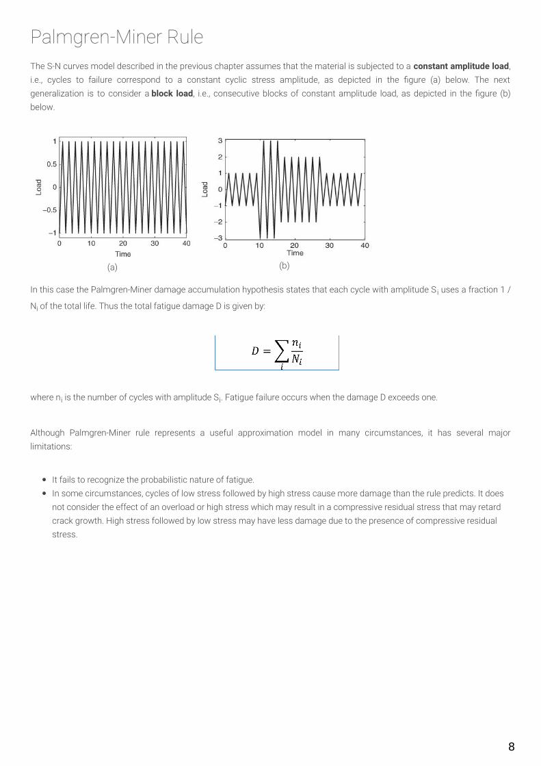
Palmgren-Miner RuleThe S-N curves model described in the previous chapter assumes that the material is subjected to a constant amplitude load,i.e., cycles to failure correspond to a constant cyclic stress amplitude, as depicted in the gure (a) below. The nextgeneralization is to consider a block load, i.e., consecutive blocks of constant amplitude load, as depicted in the gure (b)below.

(a) (b)

In this case the Palmgren-Miner damage accumulation hypothesis states that each cycle with amplitude S i uses a fraction 1 /

Ni of the total life. Thus the total fatigue damage D is given by:

where ni is the number of cycles with amplitude Si. Fatigue failure occurs when the damage D exceeds one.

Although Palmgren-Miner rule represents a useful approximation model in many circumstances, it has several majorlimitations:

It fails to recognize the probabilistic nature of fatigue.In some circumstances, cycles of low stress followed by high stress cause more damage than the rule predicts. It doesnot consider the effect of an overload or high stress which may result in a compressive residual stress that may retardcrack growth. High stress followed by low stress may have less damage due to the presence of compressive residualstress.

8

Typical Fatigue Analysis Use-CaseAlthough fatigue analysis covers a very broad range of areas, such as mechanics, physics and statistics, we can simply de neit as the process of analysing, modelling and predicting fatigue behavior. In order to summarize the fatigue analysis basics,let us consider the following example, illustrating a very simple fatigue analysis use-case in the car industry.

Suppose that a company, or some company division, is manufacturing drive shafts and a team of engineers is responsible forensuring they meet performance, quality and safety requirements. Assuming that preliminary drive shaft tests were alreadyperformed and the team is now interested in the long-term analysis, what would be the next steps?

Typically, an engineering team would rst gather as much statistical data as possible, such as target driver group (whethershafts will be used in family cars, trucks etc.), target driver behavior (average driving distance per year, average driving speedetc.), target driving conditions (road conditions, speed limits etc.) and so forth. Afterwards, statistical models describing thetarget environment would be derived. The models would, consequently, serve in a real-life testing, including real driving in thereal environment, with all the required data acquisition taking place, such as measuring load applied to the driver shaft. Finally,the cycle counting methods would be applied to the measured load signals and statistical methods, such as S-N curves orPalmgren-Miner rule, would be used to check whether load amplitudes exceed the endurance limits of the steel, how often andhow much do they exceed it, whether fatigue limit is exceeded, whether Palmgren-Miner damage is exceeded etc. If theresults would not comply with the recommended values, the shaft would probably have to undergo additional modi cationsand re-engineering.

9

Fatigue Analysis in Dewesoft XFatigue Analysis Module supports a wide range of fatigue analysis features and utils. Combined with Dewesoft X itrepresents a powerful all-in-one fatigue analysis solution allowing both acquisition and analysis of the fatigue data -everything in a single software package!

It is located under Modules → Strain, stress → Fatigue analysis, as depicted in the screenshot below.

The module is organized into three main sections: Preprocessing, Counting methods and Visualization. In fact, sectionorganization follows a typical fatigue analysis work ow that starts with the input signal preprocessing, proceeds with the cyclecounting and ends with the result visualization.

10

Remark:In acquisition mode, only the temporary fatigue analysis results (calculated only over the last block of samples) aredisplayed. In order to get the actual results (calculated over all the samples) you need to go to analyse mode and performrecalculation!

Each section represents a particular fatigue analysis stage and covers a subset of corresponding methods as follows:

1. PreprocessingTurning points filterRainflow filterDiscretization filter

2. Counting methodsRainflow counting (ASTM)Markov counting

3. VisualizationRange histogramsFrom/to matricesRange/mean matrices

11

PreprocessingThe preprocessing section includes turning points filter, rainflow filter and discretization filter.

Turning Points FilterTurning points lter detects local extrema, namely turning points, in the load signal. An example of turning point detection isdepicted in the gure (a) below. The lter is applied to the input signal by default and cannot be disabled since the FatigueAnalysis Module requires a sequence of turning points as its input (instead of a full load signal).

Rainflow FilterRain ow lter (also called the hysteresis lter) removes small oscillations from the signal, as depicted in the gure (b) below.All turning points that correspond to the cycles with the ranges below the given threshold are removed. Higher the threshold,more turning points are ltered out, and vice versa. The rain ow ltering can signi cantly reduce the number of turning points,which can be of importance for both testing and numerical simulation. Threshold parameter of value T corresponds to the T%of the absolute load signal range.

Discretization FilterDiscretization lter divides the range of a load signal into N equidistant bins and assigns each turning point to its closest bin.Figure (c) below depicts an example where signal ranging from -10 to 10 is discretized into 5 bins. Load signals are typicallyvery stochastic (please refer to the rst gure in the Fatigue Analysis Basics chapter), therefore, discretization is often appliedto make them flatter and less stochastic. The number of bins is adjusted with the Class count parameter.

Both the rain ow lter and the discretization lter are activated in the Preprocessing section by ticking the appropriate checkbox, as depicted below.

12

13

Counting Methods: Markov CountingMarkov counting is one of the most straightforward cycle counting methods. It operates on consecutive pairs of turningpoints and calculates absolute ranges between them. The method is activated by ticking the Markov counting check box inthe Algorithm settings section.

Figure below depicts an example of Markov counting in action. Clearly, the 6th turning point of the load signal is assigned avalue of |5 - 2| = 3, i.e., the absolute difference between the 6th and the 5th turning point. Similarly, the 7th turning point isassigned a value of |4 - 5| = 1, i.e., the absolute difference between the 7th and the 6th turning point.

When large amplitude cycles (such as the cycle between the 5th and the 8th turning point in the gure above) contain smalleramplitude cycles, Markov counting fails to detect them. Since large amplitude cycles play an important role in the fatigue life,this represents a major drawback of the method.

14

Counting Methods: Rainflow CountingRainflow counting is generally accepted as being the best cycle counting method up to date, and has become the industrial defacto standard. It is activated by ticking the Rainflow counting check box in the Algorithm settings section.

Remark:Currently, only ASTM compliant rain ow counting is supported. The DIN compliant is still in the testing stage but will bereleased soon.

The idea behind the method is to detect the hysteresis loops in the load signal, as depicted in the gure below. We'll refer tothe hysteresis loops as the closed cycles. Parts of the signal that do not correspond to the closed cycles are the so-calledopen cycles or residuals. Simply said, closed cycles and residuals could be visualised as full-cycles and half-cycles,respectively.

As opposed to the Markov counting, which fails to detect large amplitude cycles, the rain ow counting successfully detectsthem. As depicted in the figure below, it detects the large amplitude cycle (2,6) and the small amplitude cycle (4,5) within.

15

Different rainflow counting standards, such as ASTM, DIN and AFNOR, differ with respect to the treatment of the residuals. Inorder to be as general as possible the Fatigue Analysis Module supports both residual and non-residual mode. When Ignoreresiduals check box in the Additional algorithm settings section is checked, the residuals are omitted, otherwise they areincluded in the results.

16

VisualizationIn order to graphically represent the results the Fatigue Analysis Module uses the most common visualization techniques usedin fatigue analysis: range histograms, from/to matrices and range/mean matrices. When an input channel corresponding to aload signal of interest is selected, the following new channels are mounted:

PreprocessingPeak/valley channelRF filter channelDiscretization channel

Rainflow countingRange histogram channel (2-D)Range/mean matrix channel (3-D)From/to matrix channel (3-D)

Markov countingRange histogram channel (2-D)From/to matrix channel (3-D)

Remark:The channels marked with 2-D and 3-D correspond to 2-D and 3-D graphs, respectively. The channels corresponding to thePreprocessing section represent intermediate fatigue analysis results and serve for information purposes only.

All the channels are depicted in the screenshot below.

17

18

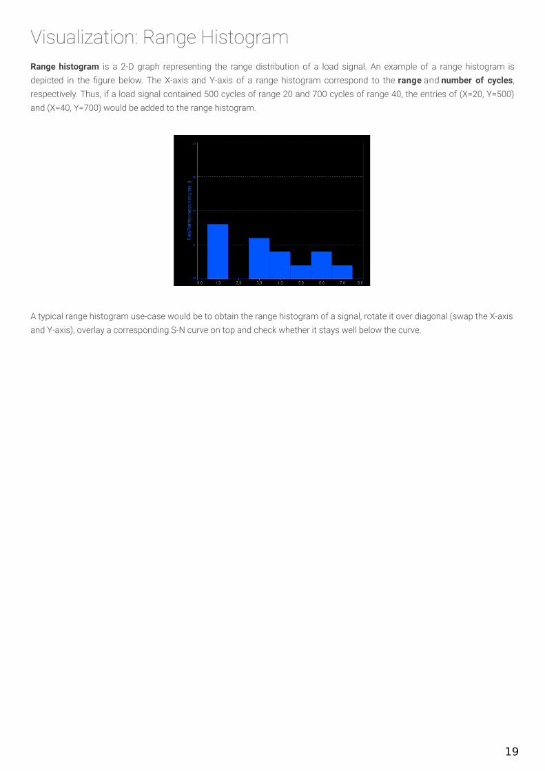
Visualization: Range HistogramRange histogram is a 2-D graph representing the range distribution of a load signal. An example of a range histogram isdepicted in the gure below. The X-axis and Y-axis of a range histogram correspond to the range and number of cycles,respectively. Thus, if a load signal contained 500 cycles of range 20 and 700 cycles of range 40, the entries of (X=20, Y=500)and (X=40, Y=700) would be added to the range histogram.

A typical range histogram use-case would be to obtain the range histogram of a signal, rotate it over diagonal (swap the X-axisand Y-axis), overlay a corresponding S-N curve on top and check whether it stays well below the curve.

19

Visualization: From/To MatrixFrom/to matrix is a 3-D graph representing the cycle distribution of a load signal. An example of a from/to matrix is depicted inthe gure below. The X-axis, Y-axis and Z-axis of a from/to matrix correspond to From (cycle minimum), To (cycle maximum)and number of cycles, respectively.

For example, the gure below depicts a cycle ranging from 5 to 10. In this case From and To are assigned the values of 5 and10, respectively. If a load signal contained 100 such cycles, an entry of (X=5, Y=10, Z=100) would be added to the from/tomatrix.

20

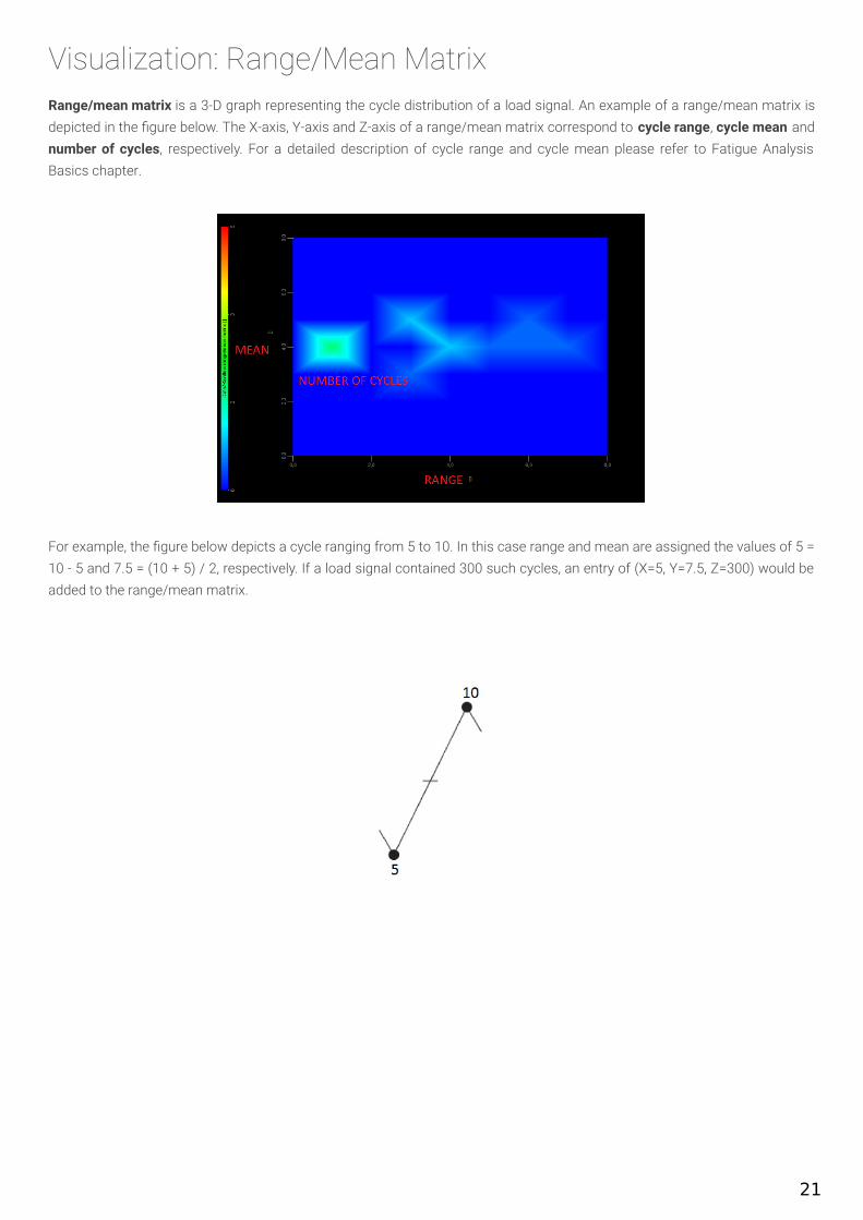
Visualization: Range/Mean MatrixRange/mean matrix is a 3-D graph representing the cycle distribution of a load signal. An example of a range/mean matrix isdepicted in the gure below. The X-axis, Y-axis and Z-axis of a range/mean matrix correspond to cycle range, cycle mean andnumber of cycles, respectively. For a detailed description of cycle range and cycle mean please refer to Fatigue AnalysisBasics chapter.

For example, the gure below depicts a cycle ranging from 5 to 10. In this case range and mean are assigned the values of 5 =10 - 5 and 7.5 = (10 + 5) / 2, respectively. If a load signal contained 300 such cycles, an entry of (X=5, Y=7.5, Z=300) would beadded to the range/mean matrix.

21

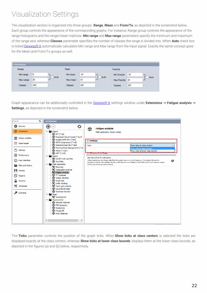
Visualization SettingsThe visualization section is organized into three groups: Range, Mean and From/To, as depicted in the screenshot below.Each group controls the appearance of the corresponding graphs. For instance, Range group controls the appearance of therange histograms and the range/mean matrices. Min range and Max range parameters specify the minimum and maximumof the range axis, whereas Classes parameter specifies the number of classes the range is divided into. When Auto check boxis ticked Dewesoft X automatically calculates Min range and Max range from the input signal. Exactly the same concept goesfor the Mean and From/To groups as well.

Graph appearance can be additionally controlled in the Dewesoft X settings window under Extensions → Fatigue analysis →Settings, as depicted in the screenshot below.

The Ticks parameter controls the position of the graph ticks. When Show ticks at class centers is selected the ticks aredisplayed exactly at the class centers, whereas Show ticks at lower class bounds displays them at the lower class bounds, asdepicted in the figures (a) and (b) below, respectively.

22

(a) (b)

23

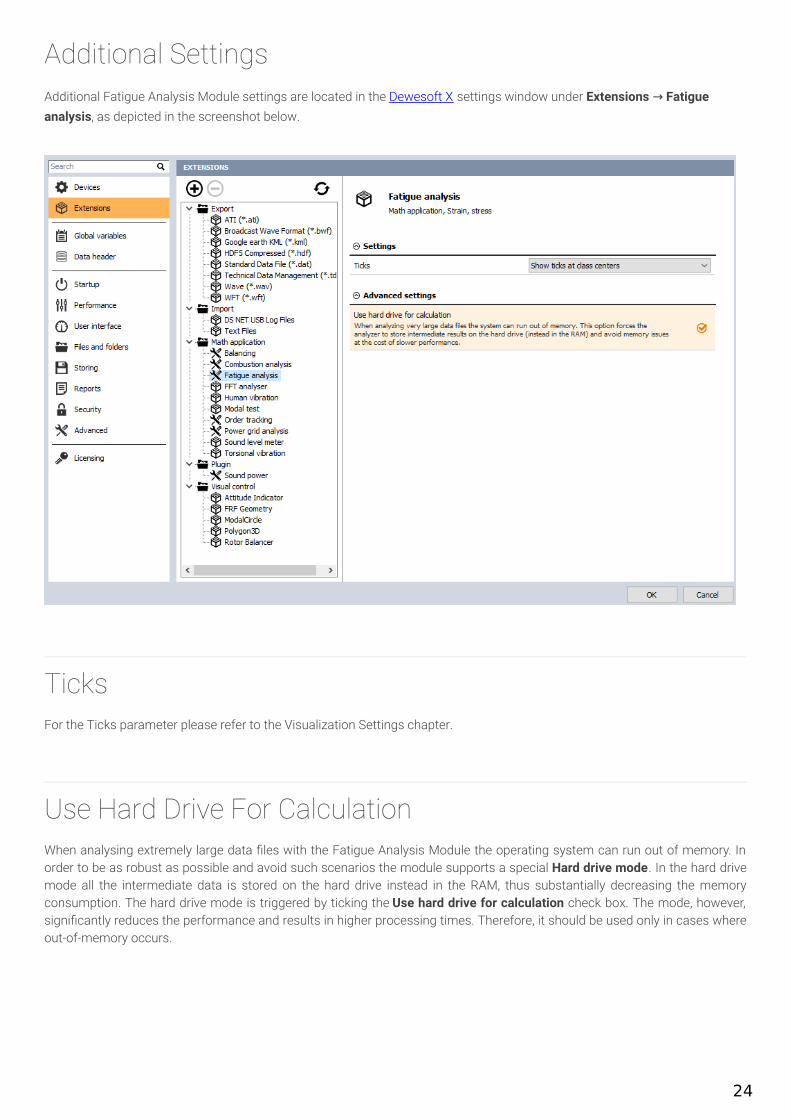
Additional SettingsAdditional Fatigue Analysis Module settings are located in the Dewesoft X settings window under Extensions → Fatigueanalysis, as depicted in the screenshot below.

TicksFor the Ticks parameter please refer to the Visualization Settings chapter.

Use Hard Drive For CalculationWhen analysing extremely large data les with the Fatigue Analysis Module the operating system can run out of memory. Inorder to be as robust as possible and avoid such scenarios the module supports a special Hard drive mode. In the hard drivemode all the intermediate data is stored on the hard drive instead in the RAM, thus substantially decreasing the memoryconsumption. The hard drive mode is triggered by ticking the Use hard drive for calculation check box. The mode, however,signi cantly reduces the performance and results in higher processing times. Therefore, it should be used only in cases whereout-of-memory occurs.

24

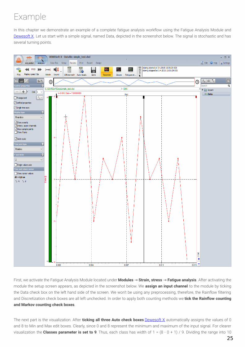
ExampleIn this chapter we demonstrate an example of a complete fatigue analysis work ow using the Fatigue Analysis Module andDewesoft X. Let us start with a simple signal, named Data, depicted in the screenshot below. The signal is stochastic and hasseveral turning points.

First, we activate the Fatigue Analysis Module located under Modules → Strain, stress → Fatigue analysis. After activating themodule the setup screen appears, as depicted in the screenshot below. We assign an input channel to the module by tickingthe Data check box on the left hand side of the screen. We won't be using any preprocessing, therefore, the Rain ow lteringand Discretization check boxes are all left unchecked. In order to apply both counting methods we tick the Rain ow countingand Markov counting check boxes.

The next part is the visualization. After ticking all three Auto check boxes Dewesoft X automatically assigns the values of 0and 8 to Min and Max edit boxes. Clearly, since 0 and 8 represent the minimum and maximum of the input signal. For clearervisualization the Classes parameter is set to 9. Thus, each class has width of 1 = (8 - 0 + 1) / 9. Dividing the range into 10

25

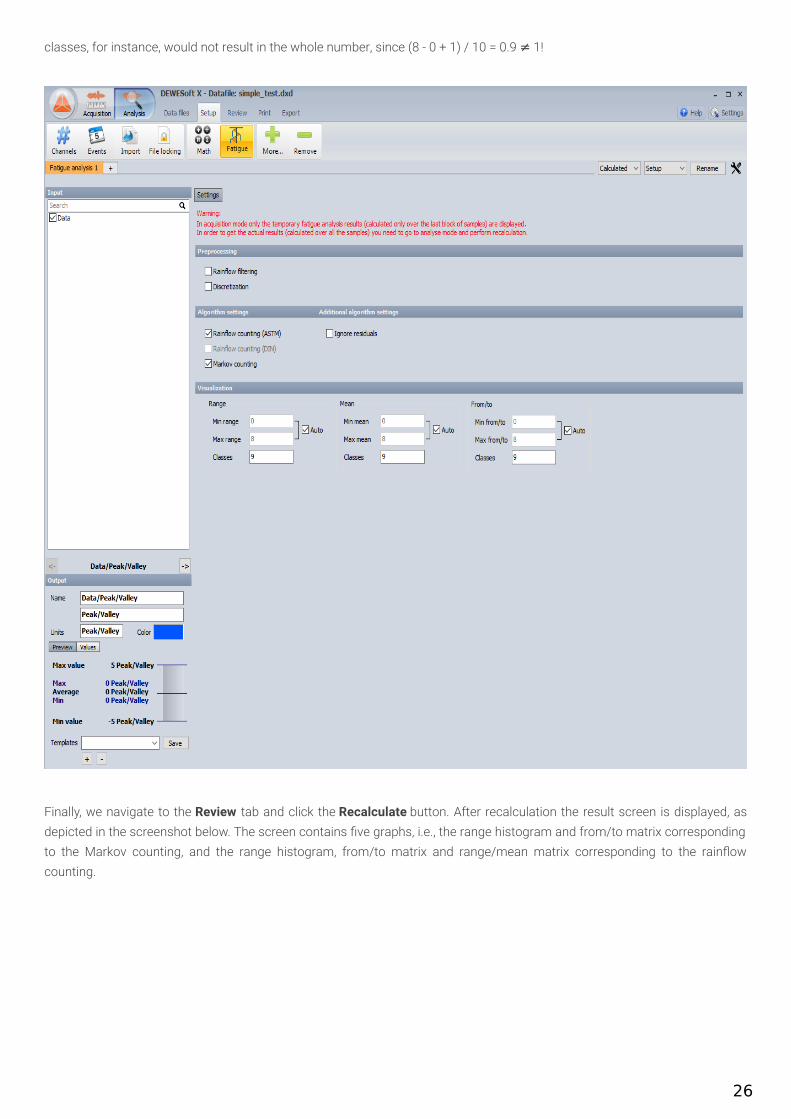
classes, for instance, would not result in the whole number, since (8 - 0 + 1) / 10 = 0.9 ≠ 1!

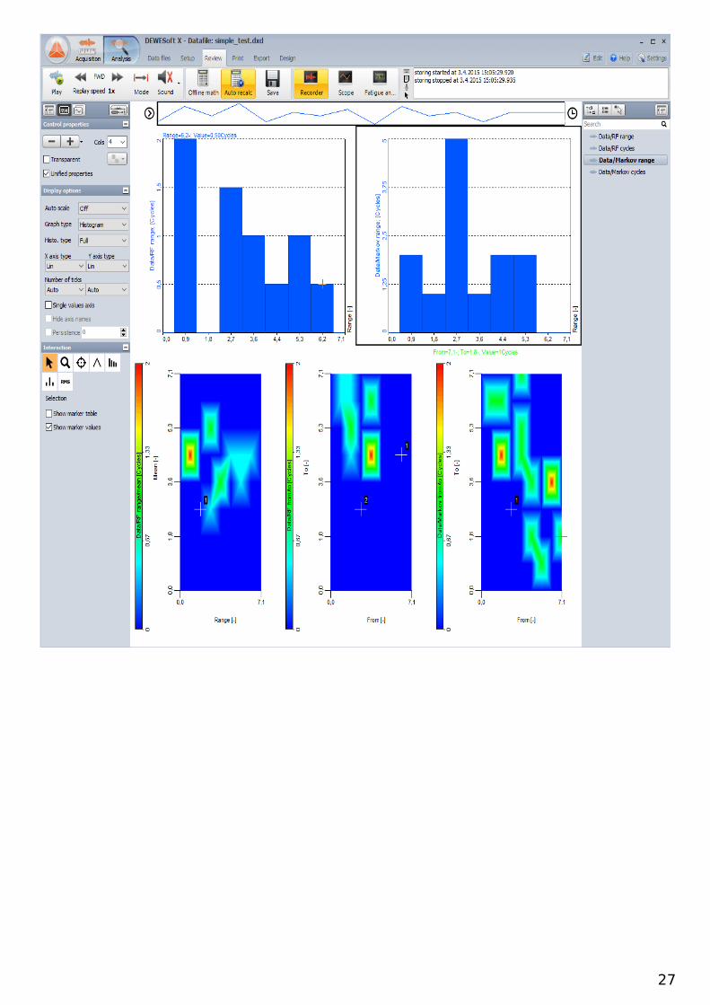
Finally, we navigate to the Review tab and click the Recalculate button. After recalculation the result screen is displayed, asdepicted in the screenshot below. The screen contains ve graphs, i.e., the range histogram and from/to matrix correspondingto the Markov counting, and the range histogram, from/to matrix and range/mean matrix corresponding to the rain owcounting.

26

27

Data ExportThe results obtained in the previous chapter can be optionally exported to a broad range of le formats. Let us, for example,export the data to a text le format. We navigate to the Export tab, as depicted in the screenshot below, and choose theText/CSV (*.text, *.csv) from the list of supported le types. After selecting the appropriate channels on the right side of thescreen, we click the Export button.

When the export has nished the exported text le appears in the Existing les list box. Double clicking the le opens it in anexternal text viewer (such as Notepad), as depicted in the screenshot below.

Remark:When a full-cycle is detected by rainflow counting it contributes a value of 1 to the total number of cycles, whereas aresidual contributes a value of 0.5. Therefore, range histograms and range/mean matrices often contain values such as0.5, 1.5, 2.5 etc. If we ticked the Ignore residuals check box the residuals would be ignored and 0.5 values would disappearfrom the results below.

28

29