fatigue in plain concretepublications.lib.chalmers.se/records/fulltext/19627.pdf · fatigue in...
TRANSCRIPT

Fatigue in Plain Concrete Phenomenon and Methods of Analysis
Master’s Thesis in the International Master’s Programme Structural Engineering
PAYMAN AMEEN & MIKAEL SZYMANSKI Department of Civil and Environmental Engineering Division of Structural Engineering Concrete Structures CHALMERS UNIVERSITY OF TECHNOLOGY Göteborg, Sweden 2006 Master’s Thesis 2006:5


MASTER’S THESIS 2006:5
Fatigue in Plain Concrete
Phenomenon and Methods of Analysis
Master’s Thesis in the International Master’s Programme Structural Engineering
PAYMAN AMEEN & MIKAEL SZYMANSKI
Department of Civil and Environmental Engineering Division of Structural Engineering
Concrete Structures CHALMERS UNIVERSITY OF TECHNOLOGY
Göteborg, Sweden 2006

Fatigue in Plain Concrete Phenomenon and Methods of Analysis Master’s Thesis in the International Master’s Programme Structural Engineering PAYMAN AMEEN & MIKAEL SZYMANSKI
© PAYMAN AMEEN & MIKAEL SZYMANSKI, 2006
Master’s Thesis 2006:5 Department of Civil and Environmental Engineering Division of Structural Engineering Concrete Structures Chalmers University of Technology SE-412 96 Göteborg Sweden Telephone: + 46 (0)31-772 1000 Cover: The figures show stress-strain diagrams obtained by using the modified Maekawa concrete model and the plasticity-damage bounding surface model. Chalmers Reproservice / Department of Civil and Environmental Engineering Göteborg, Sweden 2006

I
Fatigue in Plain Concrete Phenomenon and Methods of Analysis Master’s Thesis in the International Master’s Programme Structural Engineering PAYMAN AMEEN & MIKAEL SZYMANSKI Department of Civil and Environmental Engineering Division of Structural Engineering Concrete Structures Chalmers University of Technology
ABSTRACT
Modern concrete structures have become lighter and slender which leads to higher stress concentrations around existing initial microcracks. This fact emphasizes the importance of understanding the fracture due to cyclic loading. This type of fracture is called fatigue, which is caused by progressive, permanent internal structural changes in the material. The aim of this thesis is to give understanding and investigate the phenomenon of fatigue in plain concrete in compression. In the thesis an overview of different empirical methods is presented and two constitutive models are studied in detail on element level. In addition to the above, the thesis contains a brief review of a number of case histories, influencing factors and an introduction to constitutive modelling.
The constitutive models that were studied are the modified Maekawa concrete model and the plasticity-damage bounding surface model. In order to be tested, the models were implemented into Matlab.
The modified Maekawa concrete model is intended to be used for low-cycle fatigue while the plasticity-damage bounding surface model has the goal to be used for high-cycle fatigue. The modified Maekawa concrete model uses strain as input and is constructed in a simple way. This fact makes the implementation into FE-program easier. One disadvantage with the model is that it can not reflect deterioration due to small stress amplitudes and large number of load cycles in a proper way.
The plasticity-damage bounding surface model is more complicated. It requires a lot of computational power. The model uses stresses as input which makes it difficult to use it directly in a finite element program. The model works well for small stress amplitudes. It can describe both the loss of energy and stiffness degradation.
The models were compared with each other and the advantages and disadvantages are pointed out. The conclusion is that both models behave well only under special conditions.
Key words: Fatigue, plain concrete, cyclic loading, modified Maekawa concrete model, plasticity-damage bounding surface model, constitutive relations, constitutive modelling, concrete in compression

II
Utmattning i oarmerad betong – fenomen och analysmetoder Examensarbete inom det internationella mastersprogrammet Structural Engineering PAYMAN AMEEN & MIKAEL SZYMANSKI Institutionen för bygg- och miljöteknik Avdelningen för konstruktionsteknik Betongbyggnad Chalmers tekniska högskola
SAMMANFATTNING
Moderna betongkonstruktioner har blivit allt lättare och smäckrare. Detta medför stora spänningskoncentrationer vilket i sin tur leder till sprickor på grund av cykliska laster. Den typen av skada kallas utmattning och är orsakad av progressiva, permanenta ändringar i materialet. Målet med detta arbete är att ge en förklaring och undersöka utmattning i oarmerad betong i tryck. Olika empiriska modeller studerades, och dessutom undersöktes två konstitutiva modeller i detalj. Utöver detta innehåller rapporten en kort beskrivning av olika historiska fall då utmattning orsakade skada, några inverkande faktorer samt en introduktion till den konstitutiva modelleringen.
De konstitutiva modellerna som studerades är Maekawas modifierade betongmodell samt plasticitet och skademodell med gränsyteteori.
Meakawas modifierade betongmodell använder töjning som ingångsdata och är konstruerad på ett enkelt sätt. Detta medför att den är lätt att implementera i ett FE-program. Nackdelen med modellen är att den inte kan avspegla skada som uppstår vid högcyklisk last på ett korrekt sätt.
Plasticitet och skademodell med gränsyteteori är en komplicerad modell som kräver mycket beräkningskraft. Modellen använder spänningsökningar som ingångsdata vilket gör det svårt att implementera den i ett FE-program. Modellen fungerar bra för små spänningsamplituder.
Båda modellerna implementerades i Matlab. Modellernas för- och nackdelar beskrivs utförligt i rapporten. Slutsatsen är att modellerna fungerar korrekt endast under speciella villkor.
Nyckelord: Utmattning, oarmerad betong, cykliska laster, Maekawas modifierade betong modell, plasticitet och skademodell med gränsyteteori, konstitutiva samband, konstitutiv modellering, betong i tryck

CHALMERS Civil and Environmental Engineering, Master’s Thesis 2006:5 III
Contents ABSTRACT I
SAMMANFATTNING II
CONTENTS III
PREFACE V
NOTATIONS VI
1 INTRODUCTION 1
1.1 Background 1
1.2 Overview of the investigations about fatigue 2
1.3 Aim and Scope 2
1.4 Limitations 3
2 FATIGUE IN CONCRETE 4
2.1 Differences between concrete and steel 5
2.2 Influencing factors 6
2.3 Case histories 10
3 REVIEW OF EMPIRICAL METHODS 15
3.1 Fatigue life models 15 3.1.1 S-N curves 15 3.1.2 Goodman and Smith diagrams 16
3.2 Fatigue damage theories 17 3.2.1 Palmgren-Miner hypothesis 18 3.2.2 Modifications of PM-hypothesis 19
4 GENERAL COMMENTS ON CONSTITUTIVE MODELLING 21
4.1 The function of a constitutive model 21
4.2 Approaches for derivation and verification of a constitutive model 22 4.2.1 Fundamental approach 22 4.2.2 Phenomenological approach 24 4.2.3 Statistical approach 25
5 CONSTITUTIVE RELATIONS FOR CONCRETE IN COMPRESSION 26
5.1 Modified Maekawa concrete model 26 5.1.1 Constitutive equations 26 5.1.2 Analysis of parameters 30 5.1.3 Stresses development due to constant amplitude cyclic loading 34
5.2 Plasticity-damage bounding surface model 37 5.2.1 Constitutive equations 38

CHALMERS, Civil and Environmental Engineering, Master’s Thesis 2006:5 IV
5.2.2 Bounding surface concept 43 5.2.3 Continuum damage mechanics 45 5.2.4 Results 48
5.3 Discussion 56
6 CONCLUSIONS AND SUGGESTIONS FOR FURTHER STUDIES 57
6.1 Conclusions 57
6.2 Further studies 57
7 REFERENCES 59
APPENDIX A - Definitions
APPENDIX B - MATLAB code for the modified Maekawa concrete model
APPENDIX C - MATLAB code for the plasticity-damage bounding surface model

CHALMERS Civil and Environmental Engineering, Master’s Thesis 2006:5 V
Preface This thesis has been done at the Division of Structural Engineering at the Department of Civil and Environmental Engineering at Chalmers University of Technology. It was preceded from September 2005 to January 2006.
We wish to thank our examiner Associate Professor Karin Lundgren and our supervisor Ph.D. Candidate Rasmus Rempling for the support, supervision and advice throughout the thesis. We also wish to thank our opponents, Malin Persson and Veronica Sköld for continued assistance with the development of this thesis.
Finally, but certainly not least, we wish to thank our families who have persevered with us through our studies at Chalmers.
Göteborg, January 2006
Payman Ameen & Mikael Szymanski

CHALMERS, Civil and Environmental Engineering, Master’s Thesis 2006:5 VI
Notations Roman upper case letters A Cross-sectional area of damaged section
'A Cross-sectional area of undamaged section C Material constant
,I IIC C Compliance tensors corresponding to tensile and compressive stresses, respectively
iD Damage function
nD Damage variable
11 22 33, ,D D D The accumulated damage components in planes perpendicular to the principal axis
D Maximum value of damage accumulation
0D Accumulated damage at the beginning of each cycle
0E Coefficient = 2
0cE Young’s modulus G Shear modulus of elasticity
eH Generalize elastic shear modulus pH Generalize plastic shear modulus
1 2 3, ,I J J First, second and third stress invariant, respectively
1maxI The maximum value of the first invariant stress before current unloading K Shape factor
tK Tangent bulk modulus
0K Fracture parameter
0hK Hardening parameter N Number of cycles
iN Fatigue life at load level iL P Experimental constant PN Unloading parameter R Stress range
iS Stress level
mS Mean stress
ijS Deviatoric stress tensor
Roman lower case letters
c Intersection of the damage loading surface with the negative hydrostatic axis
d Normalized distance between current stress and the bounding surface = /δ δ
/da dN Crack growth per one loading cycle ,I IIdC dC Partial derivative with respect to the accumulated damage components
11 22 33, ,D D D
CHALMERS Civil and Environmental Engineering, Master’s Thesis 2006:5 VII
ijdD Damage growth rate
cf Uniaxial compressive strength h Damage modulus
0k The initial value of bulk tangent modulus m Material constant
in number cycles at load level iL
Greek upper case letters KΔ Stress intensity range
Greek lower case letters
β Shear compaction dilatancy factor
xβ Material constant 'β Strain rate factor = 1
δ Distance between the present stress point and the bounding surface ijδ Kronecker delta
δ Distance between the stress point on hydrostatic axis and the bounding surface
ε Total strain cε Uniaxial compressive strain
maxcε Maximum compressive strain
maxε Maximum value of principal compressive strain ever experienced
0ε Current strain ,D Ddε ε Damage strain and its increment ,e edε ε Elastic strain and its increment ,p pdε ε Plastic strain and its increment
γ Parameter describing crack geometry on the stress intensity v Poisson’s ratio θ Angle of similarity ρ Vector in plane with the deviatoric plane σ Compressive stress, effective stress
maxcσ Maximum compressive stress ,ij ijdσ σ Stress tensor and its increment
maxσ Maximum value of stress
minσ Minimum value of stress
0ccσ Current compressive stress ,σ σ+ − Positive (tensile) and negative (compressive) stresses
'σ Nominal stress 0τ Octahedral shear stress ω Strain reduction factor
ξ Hydrostatic axis


CHALMERS, Civil and Environmental Engineering, Master’s Thesis 2006:5 1
1 Introduction
1.1 Background
Concrete is a composite material consisting of three components: the cement matrix, the aggregate and the interface between the matrix and aggregate. The cement-matrix is the weakest zone of the composite. It contains voids and microcracks even before any load has been applied. Attenuation in a material or a component exposed to cyclic loading leads to increase of stress concentration around the microcracks and finally leads to fracture. Forces that are required to obtain the fracture are usually much less than forces that would have been required in case of monotonic loading. Phenomenon that deals with this type of fracture is called fatigue. It is caused by progressive, permanent internal structural changes in the material, which may result in microcracks propagation until governing macrocracks are formed. The macrocracks results in reduction of cross-section and in turn in even larger stress concentration which leads to fracture, CEB (1988).
Knowledge about fatigue is very important both from an economic point of view and from aspect of safety of the structures. Modern structures have become lighter and slender which leads to higher concentrations of stresses and to higher percentage of varying loads in comparison to the total loads. Examples of concrete structures that are exposed for cyclic loading, which causes fatigue, are roads, airfields and bridges. Another type of structures that are subjected to risk from fatigue is the modern energy-producing installations, e.g. wind power plants, offshore structures and different types of machinery foundations.
Damage due to fatigue may be divided into different categories dependent of the loading conditions as well as other e.g. environmental conditions. One defines different types of fatigue as follows:
• High-cycle fatigue: When the material requires more than 103 -104 cycles to failure then one says that the material undergoes the high-cyclic fatigue. The deterioration process is related to load frequencies.
• Low-cycle fatigue: Unlike the above, this type of fatigue is defined by a number to failure which is less than 103-104. The low-cycle fatigue is often connected to high loading amplitudes which results in loss of material stiffness.
• Thermal fatigue is a result of temperature gradient that varies with time in such a manner as to produce cyclic stresses in a material specimen. In other words the thermal fatigue is obtained when there exist rapid cycles of alternate heating and cooling. Due to expansions and extensions, crack propagation will start and the fatigue process will be accelerated significantly by increasing of temperature variation. As an example of structures where thermal fatigue occurs, power pipe lines can be mentioned.

CHALMERS, Civil and Environmental Engineering, Master’s Thesis 2006:5 2
• Corrosion fatigue: For the material specimen that is subjected to both cyclic loading and corrosive environment the failure can take place at even lower loads and after shorter time than in case of pure cyclic loading. This types of failure is denoted corrosion fatigue. The environment can have a big effect on acceleration of the fatigue process. The most usual case is spalling of concrete due to mechanical fatigue which leads to corrosion on the reinforcement.
Different combinations of the above fatigue types can also be actual. Example of such a combinations is thermomechanical fatigue i.e. combination of both varying temperature (or temperature gradient) and mechanical loading.
1.2 Overview of the investigations about fatigue
In the beginning of the industrialisation fatigue became a problem in machines and steel constructions that were subjected to cyclic loading. Failures were observed in parts where dimensions were changed. It has been founded that the parts were subjected to relatively small stresses.
The first person that started to discuss the phenomenon was German mining administrator Wilhelm Albert who in 1829 observed failure of iron mine-hoist chains. The term fatigue becomes current when French mathematician and engineer Jean-Victor Poncelet described metals as being tired during his lectures in 1839. In 1860 August Wöhler started the first systematic investigations of fatigue in railroad axles. The investigations led him to the idea of a fatigue limit and to propose the use of S-N curves in mechanical design. He found that the stress amplitude governs the fatigue strength. He discovered also that there is a fatigue limit under which no fatigue failure in steel can occur.
During the 20th century general knowledge about fatigue mechanism and behaviour in ductile material as steel, became much extended. Since about 1900 fatigue in concrete structures has been under investigation. The first article about tests on fatigue behaviour was written by Ornum (1903). The majority of the significant work has been carried out during the second half of the 20th century. However, understanding of fatigue mechanism and behaviour in brittle materials such as concrete is still lacking.
1.3 Aim and Scope
The aim of this thesis is to:
• Investigate and describe the causes of fatigue in plain concrete.
• Describe in which way different factors, e.g. different wave forms or rest periods, may influence fatigue behaviour in plain concrete.
• Describe different empirical methods that are used in order to predict life of a concrete component.

CHALMERS, Civil and Environmental Engineering, Master’s Thesis 2006:5 3
• Describe how a constitutive model, that relates stress to strain for cyclic loading, is developed.
• Evaluate and test two constitutive models describing cyclic loading in compression, in a numerical environment in order to compare the models and discuss their advantages and disadvantages.
1.4 Limitations
The master’s thesis is treating fatigue in general and constitutive models describing fatigue in plain concrete. This is due to the fact that more complex failure types in reinforced concrete structures can often be traced to the failure of plain concrete as it is in case of i.e. bending failure, shear failure of beams or bond failure of deformed bars, Gylltoft (1983). The purpose of this thesis is not to analyse the influence of structural behaviour of concrete on fatigue damage and fatigue life even though in many examples the structural behaviour is very important.
The authors describe plain concrete. However there is a short comparison between fatigue mechanisms in concrete and fatigue in steel. This is motivated by the fact that all empirical methods presented in the thesis are originally developed for analysing fatigue in steel.
The results of simulations that were made using constitutive models presented in the thesis are not compared with any experimental results. The evaluation of the models is based on deduction about how a model should work. The simulations as well as discussions about different constitutive models concern just the compressive stresses.
The models presented in this thesis are aimed for analyses of mechanical fatigue. Fatigue due to corrosion or temperature changes is not considered.

CHALMERS, Civil and Environmental Engineering, Master’s Thesis 2006:5 4
2 Fatigue in concrete Fatigue consists of progressive, internal and permanent structural changes in the material. There are different hypotheses concerning the crack initiation and propagation, e.g. according to Murdock & Kessler (1960) failure is caused by the deterioration of the bond between the coarse aggregate and the binding matrix. Another hypothesis was proposed Antrim (1967) and says that fatigue failure in plain concrete depends on small cracks that are formed in the cement paste and results in weakening of the section until it cannot sustain the applied load. However, one can conclude that fatigue in concrete is caused by microcracks, which come up due to shrinkage in hardening period. The microcracks are growing probably both at cement-matrix and aggregate interface as well as in the cement-matrix itself. Another conclusion which can be drawn is that the system of cracks is more widespread as it is in case of static loading, Holmen (1979).
Failure in concrete can be observed and modelled on three different levels as was suggested by Wittmann in 1980, according to RILEM Technical Committee 90 FMA & Elfgren (1989). This approach is called 3L-approach.
• The micro-level considers crystals of calcium silicate hydrate with primary and secondary bonds. This level is not interesting from fracture mechanics point of view, as stated by RILEM Technical Committee 90 FMA & Elfgren (1989). The behaviour at the micro-level is affected by mechanisms such as physical and chemical processes that can be active in a particular situation. The models on this level belong to material science models.
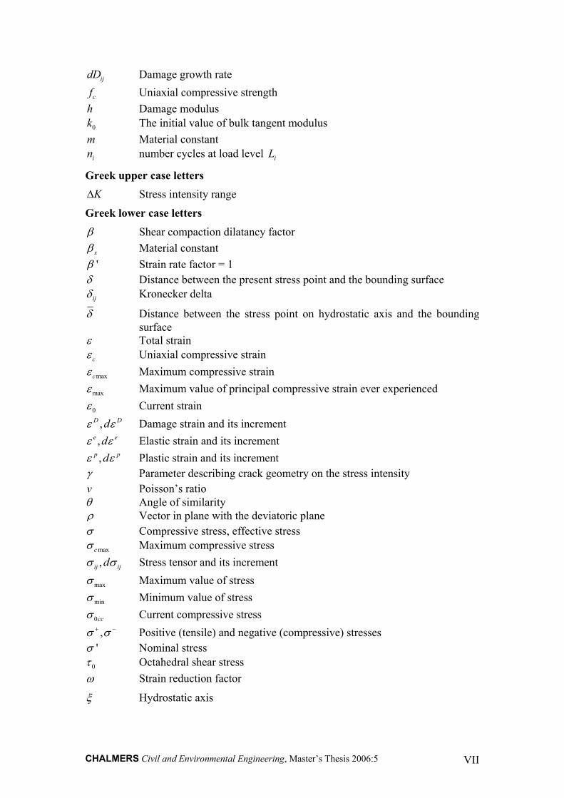
• On meso-level one considers the cement paste, aggregate and interaction between them. Reasons for failure are normally found in achieving strength of some of the following failure modes around an aggregate particle: failure of bond by tension, failure of bond by shear, failure of the matrix by tension or shear and failure of the aggregate particles, Petkovic (1991). Figure 2.1 shows typical stresses that are connected with each of the failures. The studies on this level are typically related to crack-deformation and fracture mechanism. It is observed that the average stress strain properties and non-linearity of mechanical properties will be largely influenced by acting on this level.
CHALMERS, Civil and Environmental Engineering, Master’s Thesis 2006:5 5
Figure 2.1 Local stresses around aggregate particle under tensile and compressive loading, Petkovic (1991).
• For practical applications one needs to consider also macro-level where concrete is modelled as a homogeneous isotropic material containing flaws. The properties which are interesting to study is the average strain stress properties and non-linearity of mechanical properties. The engineering models on this level should be presented in such form that can be used immediately in numerical analysis.
2.1 Differences between concrete and steel
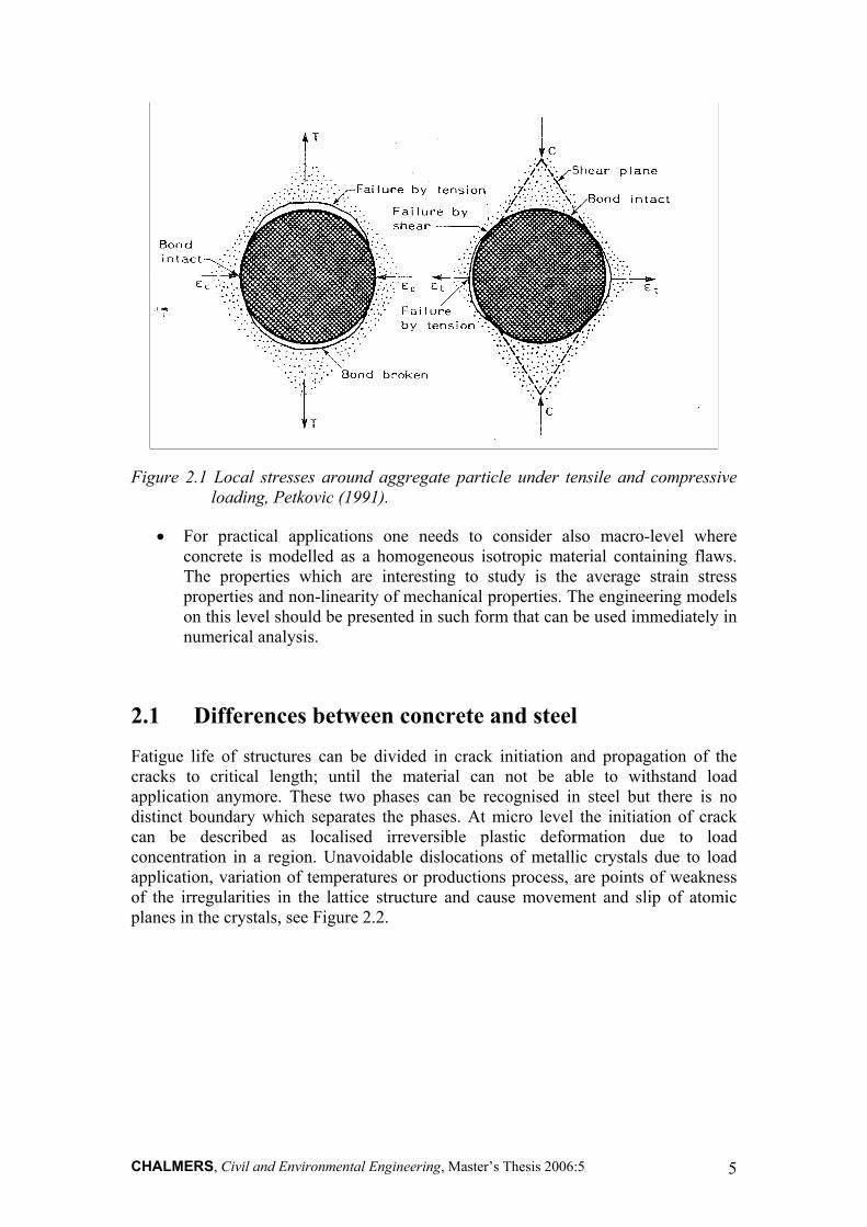
Fatigue life of structures can be divided in crack initiation and propagation of the cracks to critical length; until the material can not be able to withstand load application anymore. These two phases can be recognised in steel but there is no distinct boundary which separates the phases. At micro level the initiation of crack can be described as localised irreversible plastic deformation due to load concentration in a region. Unavoidable dislocations of metallic crystals due to load application, variation of temperatures or productions process, are points of weakness of the irregularities in the lattice structure and cause movement and slip of atomic planes in the crystals, see Figure 2.2.
CHALMERS, Civil and Environmental Engineering, Master’s Thesis 2006:5 6
Figure 2.2 Simplified modell of a cristall with an extra half atomic plane which causes a dislocation, Burström (2001).
The crack initiation in steel usually requires relatively high stress levels to develop local deformations. The crack propagation is related to the geometry of an element which is subjected to (cyclic) loading e.g. crack at weld region or crack due to local restraints has different behaviour and velocity of crack propagating.
At the first loading steel has elastic response as concrete and with increasing loading the yield surface is reached. This leads to creation of elastic (i.e. reversible) deformations and plastic (i.e. irreversible) deformations i.e. dislocation of steel crystals. Since steel material is hardening, the material endures more stress before failure. If the loading continuous until the static strength has been reached, the failure is a result.
In contrast to steel, concrete is less homogenous. This is due to voids and microcracks that come up during shrinkage caused by temperature variations during hardening period. The fatigue process starts with microcracks propagation. The cracks are growing very slowly at the beginning and rapidly at the end both in concrete and steel. In contrast steel has no any initial micro cracks of the same kind as concrete. Due to this fact as well as due to plasticity in steel, the crack growth process in steel is much slower than in concrete. While in steel it is required that cracks will be first initiated and then propagated, the failure in concrete does not require any initiation phase.
Many experiments showed that steel has a distinct fatigue limit. By fatigue limit one means the limit in the stress space below which no fatigue failure occurs. The concrete does not posses such a limiting value. The difference between steel and concrete in this case is that steel is strain hardening material and concrete is strain softening material, Gylltoft (1983). It means that the strength of steel is increasing together with large strains while the strength decreases with large strains for concrete.
2.2 Influencing factors
Fatigue strength is influenced by many different factors. Most of the experiments that were done on fatigue behavior, try to find a relation between the fatigue strength under influence of the various loading and environmental conditions. It is a common way to compare the fatigue strength obtained from the experiments with the static strength in such a way that the fatigue strength is defined as a part of static strength
CHALMERS, Civil and Environmental Engineering, Master’s Thesis 2006:5 7
for a given number of cycles. In this Chapter a number of interesting influencing factors will be presented.
Stress gradient
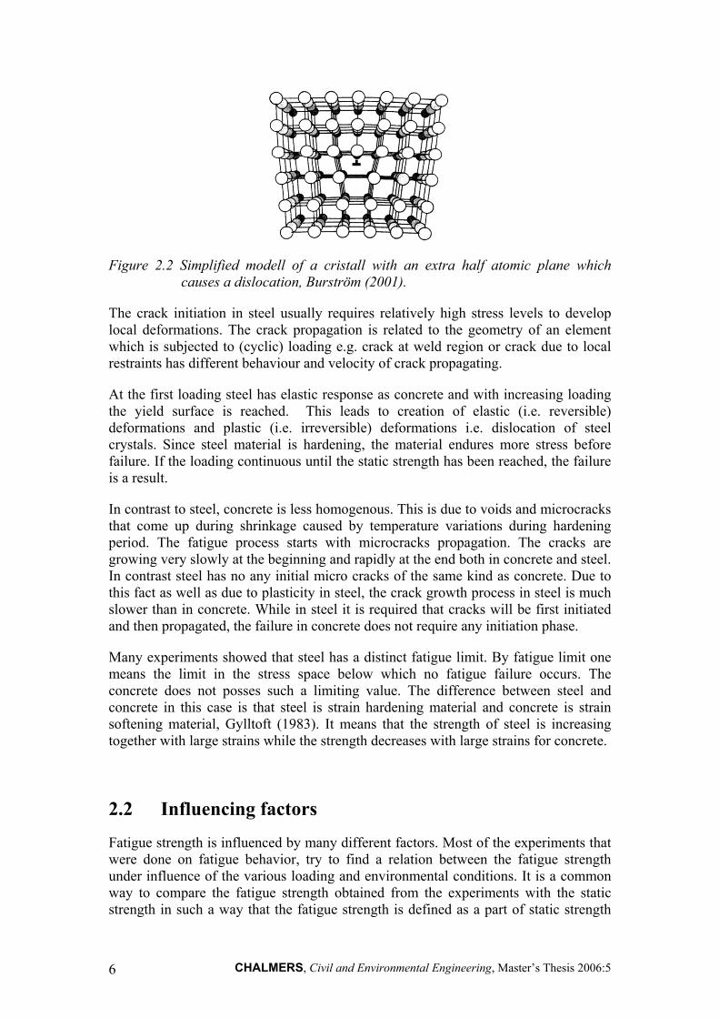
Experiments performed by Ople & Hulsbos (1966) show that static and fatigue strength are affected by eccentricity in the same degree. The experiments show that the fatigue strength in case of eccentric load increases if it is related to static strength in case of centric load. In contrast, if the eccentric cyclic load is related to static load with the same eccentricity no effect is observed, Ljungkrantz et al. (1994). Figure 2.3 shows the results of tests performed by Ople & Hulsbos (1966).
Figure 2.3 A principle drawing showing the results of tests performed by Ople & Hulsbos (1966).
Experimental tests for eccentricity presented by Cornelissen (1984) have showed that fatigue in bending gave longer fatigue life compared to fatigue in pure tension, Petkovic (1991).
Rest periods, effects of stress rate and loading frequencies
A common observation is that sequences of loading, periods without loading and periods of static loading at low stress levels increase the fatigue life of concrete. According to Hilsdorf & Kesler (1966) the rest periods up to 5 minutes can prolong the fatigue life while the longer rest periods than 5 minutes does not seem to prolong the fatigue life in additionally. Petkovic (1991) give evidence for the fact that a rest period of certain duration must be dependent on when in the loading history it occurs and which loading levels it is acting in combination with.
The maximum as well as the minimum stress (or average stress) has governing effect on fatigue life. High maximum stress will result in a shorter life length. An increase
of stress range R which is defined as min
max
R σσ
= , leads to a decrease in number of
cycles to failure. According to Abeles & American Concrete Institute; Committee 215 Fatigue of concrete (1974) this effect is especially pronounced for low stress rates.
specimen
specimen
specimen
specimen
Increased fatigue strength
No infuence
Cyclic load
Static load

CHALMERS, Civil and Environmental Engineering, Master’s Thesis 2006:5 8
Figure 2.4 shows how the number of cycles is influenced by different stress rates. The same figure shows also that the frequency of loading has little effect on the fatigue behaviour; however, a diminishing effect is manifested particularly for decreasing maximum stress level.
Petkovic (1991) has come to the conclusion that the frequency has significant effect on fatigue strength only at high stress levels. A high frequency increases the fatigue life. It follows that accelerated fatigue testing can overestimate the fatigue life.
Figure 2.4 Influence of stress rate and frequency of testing on the fatigue life of concrete, Abeles & American Concrete Institute; Committee 215 Fatigue of concrete (1974).
Different wave forms
Normally loads as wind loads or wave loads are applied in a way that the form is very similar to the sinusoidal wave, Petkovic (1991). Tepfers et al. (1973) performed an analysis of different wave shapes, e.g. sinusoidal, rectangular and triangular shapes. The result was that the rectangular wave is most damaging and triangular is least damaging. In case of rectangular wave the material is subjected to high loads during a longer time period than in case of sinusoidal or even triangular waves. Figure 2.5 shows concrete prisms that were subjected to different wave forms. The number of cycles to failure as well as waveform is shown for each prism. The time under load seems to be a factor that plays an important role. Another factor that influences the strength of the specimens subjected to different wave forms is strain velocity which is large in case of rectangular wave and small in case of triangular wave form. This emphasizes the importance of taking into account time dependent effects in concrete, when the fatigue life is calculated for different wave forms.

CHALMERS, Civil and Environmental Engineering, Master’s Thesis 2006:5 9
Figure 2.5 Tests prisms after fatigue failure, Tepfers (1980).
Lateral confining pressure
The pressure in lateral direction is considered as favorable effect on fatigue life at the lower stress levels. This is especially accentuated for lower stress levels. The relationship between mean stress Sm, stress range R and fatigue life N are shown in Figure 2.6. The influence of the positive effect of the lateral confining pressure on fatigue performance is usually lost after the specimen was loaded for more than ca. 50 times at any ratio of the lateral stress to the longitudinal in comparison to static biaxial strength, Petkovic (1991).
Figure 2.6 Fatigue life under biaxial loading, Petkovic (1991).
Effect of moisture condition
Increased moisture is a factor that influences the fatigue life of concrete in a negative way. Many experiments of various moisture conditions support this influence (e.g.
CHALMERS, Civil and Environmental Engineering, Master’s Thesis 2006:5 10
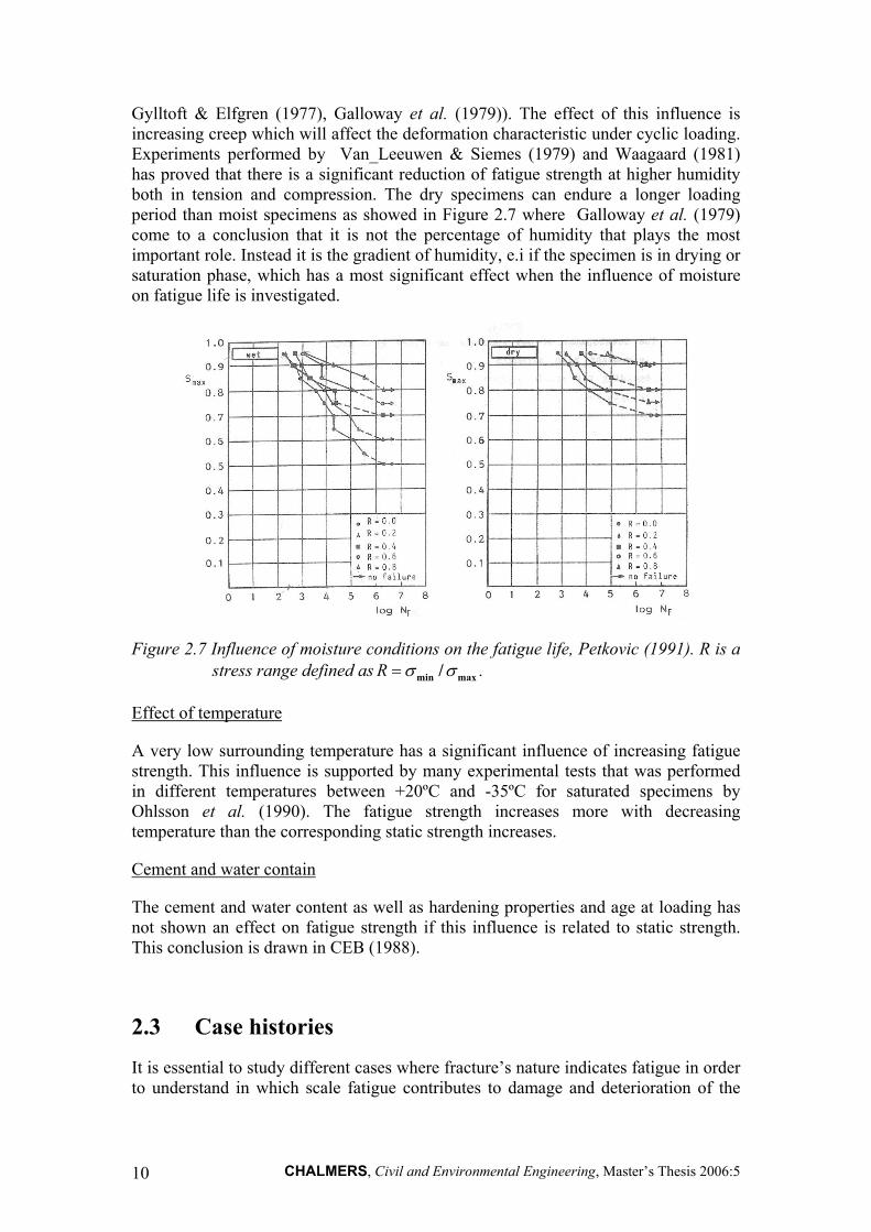
Gylltoft & Elfgren (1977), Galloway et al. (1979)). The effect of this influence is increasing creep which will affect the deformation characteristic under cyclic loading. Experiments performed by Van_Leeuwen & Siemes (1979) and Waagaard (1981) has proved that there is a significant reduction of fatigue strength at higher humidity both in tension and compression. The dry specimens can endure a longer loading period than moist specimens as showed in Figure 2.7 where Galloway et al. (1979) come to a conclusion that it is not the percentage of humidity that plays the most important role. Instead it is the gradient of humidity, e.i if the specimen is in drying or saturation phase, which has a most significant effect when the influence of moisture on fatigue life is investigated.
Figure 2.7 Influence of moisture conditions on the fatigue life, Petkovic (1991). R is a stress range defined as R σ σ= min max/ .
Effect of temperature
A very low surrounding temperature has a significant influence of increasing fatigue strength. This influence is supported by many experimental tests that was performed in different temperatures between +20ºC and -35ºC for saturated specimens by Ohlsson et al. (1990). The fatigue strength increases more with decreasing temperature than the corresponding static strength increases. Cement and water contain
The cement and water content as well as hardening properties and age at loading has not shown an effect on fatigue strength if this influence is related to static strength. This conclusion is drawn in CEB (1988).
2.3 Case histories
It is essential to study different cases where fracture’s nature indicates fatigue in order to understand in which scale fatigue contributes to damage and deterioration of the

CHALMERS, Civil and Environmental Engineering, Master’s Thesis 2006:5 11
infrastructure. In this chapter a brief description of different, interesting case histories is made. The cases are selected from CEB (1988).
All examples show clearly that the phenomenon of pure fatigue cannot be isolated as the only reason for deterioration. Most of examples are coupled with other events e.g. repeated deflections, increased loading, and increased frequencies or vibrations. Other events that can magnify the deterioration caused by fatigue are chemical attack as fretting, pitting or carbonation attack, particularly in prestressed concrete, CEB (1988).
Japanese bridge decks
Since 1965 there have been numerous instances of fatigue failures in reinforced concrete bridge decks. Several signs of fracture were observed: spalling of concrete below the bottom layer of reinforcement at the soffit or/and depressions of the running surface due to punching failure. No failure in steel has been noticed. The damage interfered with the serviceability just after a few years of usage. The main reason of damage was created from increasing and repeated passage of wheel loads. Many investigations have showed that the problem has arisen partly from design procedures. The engineers did not take into account the fatigue aspects and they did not consider possibility of increasing traffic load. This failure is classified today as a fatigue failure which origins from repeated shear and tensional effects on the structure that reduces the strength. Similar failure has also been observed in bridges in Sweden.
Bridge decks in Holland
Between 1935 and 1950 about thirty trussed-girder bridges were built in Holland. These bridges have reinforced concrete decks which are supported by longitudinal and transverse steel beam. Concrete was cast in situ on the steel beam but there was no structural connection to the beam. Since then all the concrete decks have been replaced because of very many small cracks that were leading to total disintegration of concrete. In early stage of service life longitudinal cracks on bridge decks under the wheel tracks have been observed. Again no damage to reinforcement has been noticed. Durability of the deck is clearly depending on intensity of the traffic. The bridge was designed according to the Dutch codes which had no rules for fatigue design at the time.
Bridge over Tärnaforsen, Sweden
The fatigue cracking problems started on one occasion during the 1950’s when a 2200 kN heavy transformer was taken over bridge. After that incident the permissible load was exceeded many times by timber trucks crossing the bridge but the investigators assumes that fatigue fructure have started since the first incident. After many researches it has been proved that the bridge contains insufficient shear reinforcement. Thus the shear resistance is uncomplete. The cracks were repaired but have returned. Before the 1960´s one believed that concrete had greater shear resistance. Figure 2.8 presents the recorded cracks in the bridge over Tarnaforsen. The upper part of the

CHALMERS, Civil and Environmental Engineering, Master’s Thesis 2006:5 12
figure shows the upstream side of the brigde while the lower part shows the downstream side. The most cracks arrised in the middle of each span.
Figure 2.8 Recorded cracks in main concrete beam with 4 spans. Road E79, Bridge Ume River at Tärnafors, Tärnaby-Storuman, CEB (1988).
Travelling crane track, Sweden
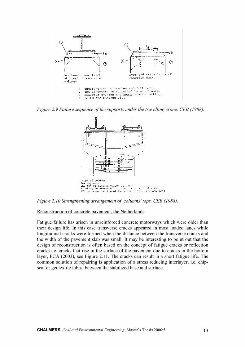
In structures that contains a permanent travelling crane the common solution is that the track structure rests on nuts that transfers the loads to concrete columns through hold down bolts and mortar under the steel members. Track that was built in 1976 in Sweden just after a few years of usage one could observe spalling of the concrete around the bolts and cracks in mortar. The cracks propagation led finally to shearing off the bolts. Figure 2.9 shows this event. It was concluded that the damage have been caused by repeated loads from the crane. The tops of the columns were repaired with reinforcement and since then the structure performed well. Figure 2.10 shows the strengthening arrangement of the repaired columns tops.
CHALMERS, Civil and Environmental Engineering, Master’s Thesis 2006:5 13
Figure 2.9 Failure sequence of the supports under the travelling crane, CEB (1988).
Figure 2.10 Strengthening arrangement of columns' tops, CEB (1988).
Reconstruction of concrete pavement, the Netherlands
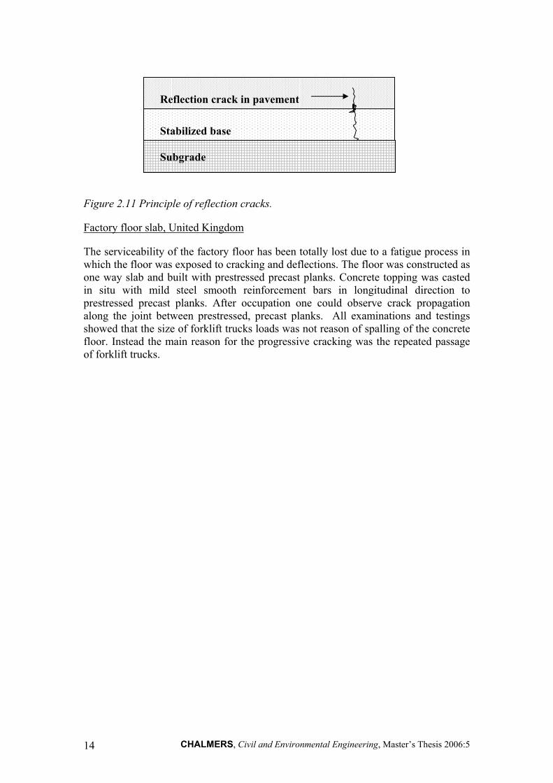
Fatigue failure has arisen in unreinforced concrete motorways which were older than their design life. In this case transverse cracks appeared in most loaded lanes while longitudinal cracks were formed when the distance between the transverse cracks and the width of the pavement slab was small. It may be interesting to point out that the design of reconstruction is often based on the concept of fatigue cracks or reflection cracks i.e. cracks that rise in the surface of the pavement due to cracks in the bottom layer, PCA (2003), see Figure 2.11. The cracks can result in a short fatigue life. The common solution of repairing is application of a stress reducing interlayer, i.e. chip-seal or geotextile fabric between the stabilized base and surface.
CHALMERS, Civil and Environmental Engineering, Master’s Thesis 2006:5 14
Figure 2.11 Principle of reflection cracks.
Factory floor slab, United Kingdom
The serviceability of the factory floor has been totally lost due to a fatigue process in which the floor was exposed to cracking and deflections. The floor was constructed as one way slab and built with prestressed precast planks. Concrete topping was casted in situ with mild steel smooth reinforcement bars in longitudinal direction to prestressed precast planks. After occupation one could observe crack propagation along the joint between prestressed, precast planks. All examinations and testings showed that the size of forklift trucks loads was not reason of spalling of the concrete floor. Instead the main reason for the progressive cracking was the repeated passage of forklift trucks.
Stabilized base
Reflection crack in pavement
Subgrade

CHALMERS, Civil and Environmental Engineering, Master’s Thesis 2006:5 15
3 Review of empirical methods The investigation methods of fatigue can generally be divided into life prediction methods based on probabilistic theories as well as stress and strain based methods, which comes into constitutive relations. In Chapter 3.1 a short summary of the fatigue life models based on empirical data will be presented. The summary is not a complete overview of the existing life prediction models; only the models that have been used and are suggested as a basis in the codes will be given, Johansson (2004). Chapter 3.2 presents fatigue damage theories that can be used when more complicated loading histories are studied.
It should be noted that also Paris’ law, which is not an empirical method, is often used in fatigue analyses. Paris’ law describes crack growth in the material. The following equation describes Paris’ law:
mKCdNda )(Δ=
(3.1)
In the above equation, da/dN is the crack growth per one load cycle, ΔK is the stress intensity range during the same load cycle while C is a constant and m is a slope on log-log plot, assuming of course that decades on both log scales are the same length. The constant m is a material constant. The modifications of Paris’ law are often concerning the materials constant C and m. These parameters can be chosen as functions, rather than constants.
3.1 Fatigue life models
As already stated, the fatigue strength is commonly defined as fraction of static strength that can be supported repeatedly for a given number of cycles. It can be represented by fatigue life curves, referred to as S-N curves. Another way to show fatigue life is by using Goodman or Smith diagrams. The diagrams represent the dependence of maximum and minimum stress on fatigue strength.
3.1.1 S-N curves
In high-cycle fatigue situations, materials performance is commonly characterized by an S-N curve, also known as the Wöhler curve. The S-N curves are showing the relation between constant stress amplitude applied to the material and the number of cycles that leads to failure.
In order to obtain the curve, each of the tested specimens is exposed to a cyclic loading with constant amplitude. Then the number of cycles until failure in the specimen is observed. The logarithm of the number of load cycles to failure, N, at a specific maximum stress level, σmax is plotted in a diagram. One such a curve is valid for a constant ratio between maximum and minimum stress. To obtain statistically reasonable information for each curve, it is necessary to test several specimens at each

CHALMERS, Civil and Environmental Engineering, Master’s Thesis 2006:5 16
stress level due to the fact that the fatigue tests usually give a large scatter in number of cycles to failure. By applying probabilistic procedures, required probability of failure at specific number of cycles to failure can be obtained, as described by Johansson (2004). The experimental procedure is sometimes known as coupon testing.
From S-N curves one can obtain information about the fatigue limit or its deficiency. Figure 3.1 shows a typical Wöhler curve for concrete in compression. As have been stated in Chapter 2.1, concrete lacks a fatigue limit. This can be observed in the fact that the S-N curves for concrete are straight lines which do not converge to any specific value on the vertical axis for large number of cycles.
Figure 3.1 Typical S-N line for constant R-values, according to Johansson (2004).
Often σmax is related to permanent and variable load while σmin is composed of just a permanent load. A relation between number of cycles to failure and maximum stress is possible to express by the following formula according to Gylltoft (1983):
max1log ( )(0.93 )0.043 c
Nf
σ= −
(3.2)
3.1.2 Goodman and Smith diagrams
A different way to predict life length is to use a Goodman diagram. The Goodman diagram is a diagram where the maximum stress level σmax is denoted on the vertical axis while the minimum stress σmin is on the horizontal axis. Different lines represent

CHALMERS, Civil and Environmental Engineering, Master’s Thesis 2006:5 17
different numbers of cycles to failure. A typical Goodman diagram is shown in Figure 3.2.
Figure 3.2 Goodman diagram given for different numbers of cycle N, according to Johansson (2004).
A similar way of representing number of cycles to failure is by using the Smith diagram. In this diagram both the maximum and minimum stresses are instead on vertical axis and the mean stress is on the horizontal axis.
If the ratio between minimum and maximum stresses, R, is included in the S-N-relationship, both the Wöhler and the Goodman/Smith diagrams can be expressed in one equation. As an example the equation presented in Johansson (2004) is presented below:
max 1 (1 ) logx R Nσ β= − − (3.3)
where βx is a material constant between 0.064 to 0.080, Johansson (2004).
3.2 Fatigue damage theories
Due to the fact that a usual loading history consists of varying amplitude and varying number of cycles, the influence of these changing loading characteristics is often considered by using the linear damage hypotheses, as in Palmgren-Miner hypothesis.
CHALMERS, Civil and Environmental Engineering, Master’s Thesis 2006:5 18
3.2.1 Palmgren-Miner hypothesis
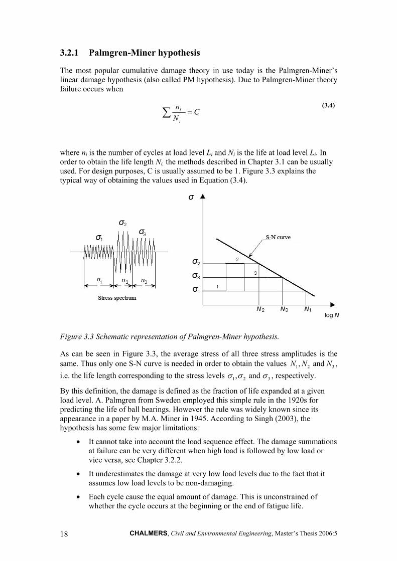
The most popular cumulative damage theory in use today is the Palmgren-Miner’s linear damage hypothesis (also called PM hypothesis). Due to Palmgren-Miner theory failure occurs when
CNn
i
i =∑ (3.4)
where ni is the number of cycles at load level Li and Ni is the life at load level Li. In order to obtain the life length Ni, the methods described in Chapter 3.1 can be usually used. For design purposes, C is usually assumed to be 1. Figure 3.3 explains the typical way of obtaining the values used in Equation (3.4).
Figure 3.3 Schematic representation of Palmgren-Miner hypothesis.
As can be seen in Figure 3.3, the average stress of all three stress amplitudes is the same. Thus only one S-N curve is needed in order to obtain the values 1 2 3, and N N N , i.e. the life length corresponding to the stress levels 1 2 3, and σ σ σ , respectively.
By this definition, the damage is defined as the fraction of life expanded at a given load level. A. Palmgren from Sweden employed this simple rule in the 1920s for predicting the life of ball bearings. However the rule was widely known since its appearance in a paper by M.A. Miner in 1945. According to Singh (2003), the hypothesis has some few major limitations:
• It cannot take into account the load sequence effect. The damage summations at failure can be very different when high load is followed by low load or vice versa, see Chapter 3.2.2.
• It underestimates the damage at very low load levels due to the fact that it assumes low load levels to be non-damaging.
• Each cycle cause the equal amount of damage. This is unconstrained of whether the cycle occurs at the beginning or the end of fatigue life.

CHALMERS, Civil and Environmental Engineering, Master’s Thesis 2006:5 19
3.2.2 Modifications of PM-hypothesis
One of the first attempts to obtain a damage function by use of PM-hypothesis was made by Marco & Starkey (1954). A modification of PM-hypothesis shows that the damage accumulation caused by constant amplitude loading is of a non-linear nature. According to Marco & Starkey (1954), the damage function Di at stress level Si can be expressed as
( ) ixii
i
nDN
= (3.5)
where x depend on the stress level as indicated in Figure 3.4.
Figure 3.4 Stress-dependent damage/cycle ratio relationship, Holmen (1979).
Hilsdorf & Kesler (1966) performed tests with PM-hypothesis on two stage constant amplitude loading. They have concluded that the sum of the cumulative damage is greater than one when the magnitude of the first stage is smaller than the second one and the damage cumulative is less one when the magnitude of the first sequence is larger than the second as shown below, e.g.:
1 2
1 2
1i
i
n n nN N N= + <∑ for the loading sequence shown in Figure 3.5
1 2
1 2
1i
i
n n nN N N= + >∑ for the loading sequence shown in Figure 3.6
1.0
1.0 Cycle ratio n/N
Dam
age
D
Palmgren-Miner
S1
S2
S3
CHALMERS, Civil and Environmental Engineering, Master’s Thesis 2006:5 20
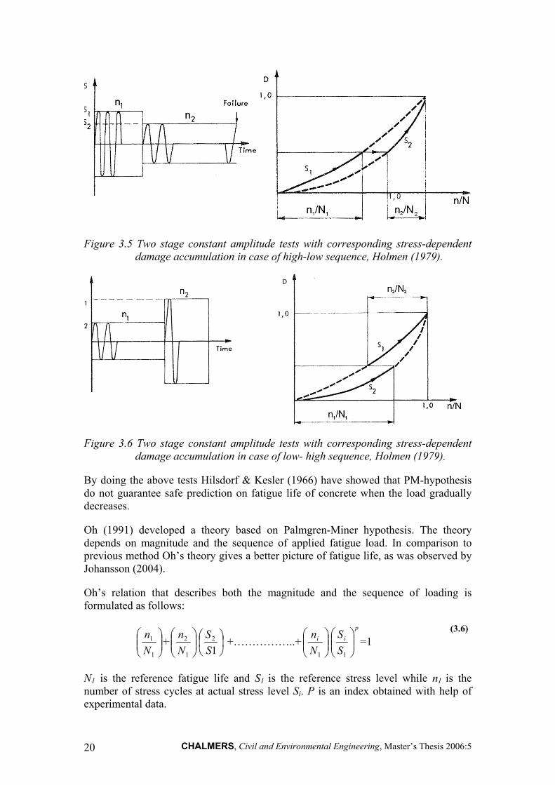
Figure 3.5 Two stage constant amplitude tests with corresponding stress-dependent damage accumulation in case of high-low sequence, Holmen (1979).
Figure 3.6 Two stage constant amplitude tests with corresponding stress-dependent damage accumulation in case of low- high sequence, Holmen (1979).
By doing the above tests Hilsdorf & Kesler (1966) have showed that PM-hypothesis do not guarantee safe prediction on fatigue life of concrete when the load gradually decreases.
Oh (1991) developed a theory based on Palmgren-Miner hypothesis. The theory depends on magnitude and the sequence of applied fatigue load. In comparison to previous method Oh’s theory gives a better picture of fatigue life, as was observed by Johansson (2004).
Oh’s relation that describes both the magnitude and the sequence of loading is formulated as follows:
⎟⎟⎠
⎞⎜⎜⎝
⎛
1
1
Nn + ⎟⎟
⎠
⎞⎜⎜⎝
⎛
1
2
Nn
⎟⎠⎞
⎜⎝⎛
12
SS +……………..+ ⎟⎟
⎠
⎞⎜⎜⎝
⎛
1Nni
p
i
SS⎟⎟⎠
⎞⎜⎜⎝
⎛
1
=1 (3.6)
N1 is the reference fatigue life and S1 is the reference stress level while n1 is the number of stress cycles at actual stress level Si. P is an index obtained with help of experimental data.

CHALMERS, Civil and Environmental Engineering, Master’s Thesis 2006:5 21
4 General comments on constitutive modelling In order to describe any problem in continuum or solid mechanics, one needs to consider three characteristics of the problem: the Newtonian equation of motion, the geometry of deformation and the stress-strain relation which is specific for the considered material.
The equation of motion casts light on the relation between the forces acting on a body and the motion of a body. The more general form of this relation expresses the conservation of linear and angular momentum as well as the related concept of stress. The conservation of linear momentum, which is a product of the mass of an object and its velocity, says that this quantity never changes in an isolated collection of objects. The conservation of angular momentum, which describes the rotational motion, is somewhat more complicated but basically it describes the issues connected with the rotational motion in the same way as linear momentum describes linear motion. Due to this more general form of Newtonian equations of motion, that was recognized by Euler and formalized by Cauchy, Britannica (2005), it is possible to apply the laws to finite bodies and not just to point particles.
The second characteristic which describes the geometry of deformations of a body is in a more general term called kinematics. It is a subdivision of classical mechanics that concerns the geometrically possible motion and deformations of a body. Through geometrical relations the expression of strains in terms of gradients in the displacement field can be described.
In order to connect the above two characteristics the third characteristic is needed. This is called the constitutive relation and can be regarded, from a mathematical point of view, as complementary equation to the balance and kinematics equations. Figure 4.1 shows an illustrative formulation of the relations between the above mentioned characteristics.
Figure 4.1 Flow scheme showing relations between different characteristics of a problem in continuum or solid mechanics.
4.1 The function of a constitutive model
In order to describe a material with help of a constitutive relation, a theory that is adequately in a given situation must be selected. Due to the fact that the different
P σ
ε p
Equilibrium relations
Kinematics Con
stitu
tive
rela
tions
P – forces
σ – stresses
ε – strains
p - deformations

CHALMERS, Civil and Environmental Engineering, Master’s Thesis 2006:5 22
models are just approximations of complicated physics that is lying behind the performance of materials, there exists no exact model that can describe everything. Different purposes requires different model. A few examples of different types of models that are relevant for different aims are reviewed below, according to Runesson (2005):
• Structural analysis under working load (before cracking): Linear elasticity.
• Analysis of damped vibrations: Viscoelasticity.
• Accurate calculation of permanent deformation after monotonic or cyclic loading: Hardening elasto-plasticity.
• Analysis of high-cycle fatigue: Damage coupled to elastic deformations.
• Analysis of low-cycle fatigue: Damage coupled to plastic deformations.
In structural analysis, when concrete cracks or gets close to failure, crack models based on fracture mechanics and plasticity models are usually used.
With the intention of making the analysis of structural component efficient, one must on forehand verify that the chosen model is sufficient to describe the physical phenomena, produce sufficiently accurate predictions for the given purpose and be capable to be implemented into a computer code designated for structural analysis, Runesson (2005). The verification of these three aspects is the most strenuous part of creation of a new model, but also the most arduous part of verification of an existing model.
4.2 Approaches for derivation and verification of a constitutive model
Runesson (2005) describes three conceptually different approaches to derive a constitutive model. These are fundamental approach, phenomenological approach, and statistical approach. In this subchapter the authors give an introduction to these three different approaches.
4.2.1 Fundamental approach
By reason of the declaration that this approach uses a microstructural behaviour as a basis to derive a constitutive relation, this approach demands a detailed knowledge about the deformation and failure characteristics. With the purpose of establishing a useful macroscopic model, different homogenization techniques (i.e. averaging the response of the material from micro to macro scale) can be used. A general, numerical line of attack in order to obtain a homogenization is carried out by usage of a Representative Volume Element (further called RVE or RV element). There are different descriptions of how the RV element should be defined. One objective which is common in all definitions is the statement that the RVE should be adequately large
CHALMERS, Civil and Environmental Engineering, Master’s Thesis 2006:5 23
to admit statistical representation of the material but still small enough to represent a dimensionless point. Three different definitions are discussed below.
According to Shan & Gokhale (2002), the first formal definition of RVE says that a RVE must be structurally entirely typical for the whole micro-structure on average as well as it must contain a sufficiently number of heterogeneities for an apparent overall modulus to be effectively independent of the surface values of traction an displacement, as long as these values are microscopically uniform.
Another definition says that a RV element should be chosen as the smallest volume element of a material for which the usual spatially constant overall modulus is sufficiently accurate to represent overall constitutive response.
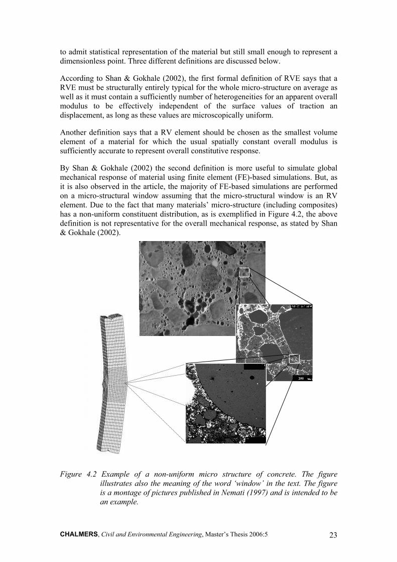
By Shan & Gokhale (2002) the second definition is more useful to simulate global mechanical response of material using finite element (FE)-based simulations. But, as it is also observed in the article, the majority of FE-based simulations are performed on a micro-structural window assuming that the micro-structural window is an RV element. Due to the fact that many materials’ micro-structure (including composites) has a non-uniform constituent distribution, as is exemplified in Figure 4.2, the above definition is not representative for the overall mechanical response, as stated by Shan & Gokhale (2002).
Figure 4.2 Example of a non-uniform micro structure of concrete. The figure illustrates also the meaning of the word ‘window’ in the text. The figure is a montage of pictures published in Nemati (1997) and is intended to be an example.
CHALMERS, Civil and Environmental Engineering, Master’s Thesis 2006:5 24
Instead Shan and Gokhale propose their own definition of an RV element. The following is the basic characteristic of their own definition:
(i) micromechanical responses of the window is statically similar to those of a macrosize specimen of the same material,
(ii) the properties as well as micro-stresses and –strains of the window do not vary with the location of the window,
(iii) different realization of the simulated micro-structure window have similar micro-structure and micro-mechanical response and
(iv) the micro-mechanical response of the window is unique for a given loading direction although different loading directions may yield different micro-mechanical response due to non-uniform nature of the micro-structure.
According to simulations performed in Shan & Gokhale (2002), this definition gives realistic results that can reflect the changes in the micro-structure.
A more powerful method of homogenization, by means of Runesson (2005), is a Computational Multiscale Modelling (CMM). Instead of simulating the response of the RVE itself, one chooses here to simulate the RVE’s response as an integrated part of the macroscopic analysis of a given component. This way of deriving or testing a constitutive model requires, though, the global balance equations of mechanics.
4.2.2 Phenomenological approach
The word phenomenalism describes a theory which states that all knowledge is of phenomena and that what is construed to be perception of material objects is simply perception of sense-data. With other words the propositions about material objects are reduced to propositions about actual and possible appearances only.
By means of material performance’s modelling the phenomenological approach supports the model on the observed characteristics from elementary tests. According to Runesson (2005) the calibration of a model is then carried out by comparison of experimental data and/or with micro mechanical predictions for well-defined boundary conditions on the relevant RV element.
In order to optimize a predictive capability of the model in question, the objective function has to be minimized with respect to the difference between the predicted response and the experimentally obtained data.
Experiments are needed for obtaining test results and statistics. There exists well-defined laboratory experiments with standardized results; these are e.g. uniaxial stress, normal stress combined with shear, cylindrical stress, and strain states or true triaxial stress and strain states. All these test have one common idea, namely that the specimen under consideration is subjected to homogeneous states of stresses, strain and temperature.

CHALMERS, Civil and Environmental Engineering, Master’s Thesis 2006:5 25
4.2.3 Statistical approach
In the statistical approach the models are based on the response of certain structures or specimens, specific loading conditions and given environmental conditions. Thus, these kinds of models are least suited to describe arbitrary appearances and to predict future responses of a material for random boundary conditions such as loads, geometry, etc. Most often used distribution that describes the scatter in strength data is Weibull’s statistical theory, Runesson (2005).
CHALMERS, Civil and Environmental Engineering, Master’s Thesis 2006:5 26
5 Constitutive relations for concrete in compression
In this Chapter two constitutive models are presented; the modified Maekawa concrete model and a plasticity-damage bounding surface model by Abu-Lebdeh (1993). The reason of the choice of these two models is that they work in quite different ways and have very different construction. Thus, it seems interesting to explore and compare them. The models are relatively new. The modified Maekawa concrete model was developed in the beginning of 21st century while the plasticity damage bounding surface model was developed in the last decade of 20th century. In order to test them numerically, the models were implemented in Matlab. The analysis of the models are followed by a discussion about the relevance and applicability.
5.1 Modified Maekawa concrete model
The modified Maekawa concrete model has been developed by the research group of professor Maekawa at Tokyo University. The proposed model is a part of the orthogonal two-way fixed crack model. The model uses different constitutive equations to describe the behavior of concrete before and after cracking of concrete, see Maekawa et al. (2003). The constitutive relations formulated in the model are addressed to the concrete model under a strain rate of approximately 10-4-10-3/sec, which makes it appropriate for dynamic analysis under earthquakes loads. The parameters used in Maekawa concrete model are proposed for concrete with normal aggregate and strength ranging from 15 MPa to 50 MPa. The model is used in DIANA 9 - software that is intended to finite element analysis of e.g. concrete structures - as a triaxial model. The implementation in DIANA of the effects of cyclic loading is called the ‘Modified Maekawa’ concrete model.
5.1.1 Constitutive equations
In this Chapter the equations of the uniaxial compression model parallel to the crack direction are studied. The modified Maekawa concrete model uses engineering parameters as compressive and tensile strength. Here the model is implemented and tested in Matlab. In the following analyses deformation control was used. Thus, the strain increment is used as an input in the Matlab program.
The model is an elasto-plastic fracture (EPF) model. The concept of the EPF model is shown in Figure 5.1.
CHALMERS, Civil and Environmental Engineering, Master’s Thesis 2006:5 27
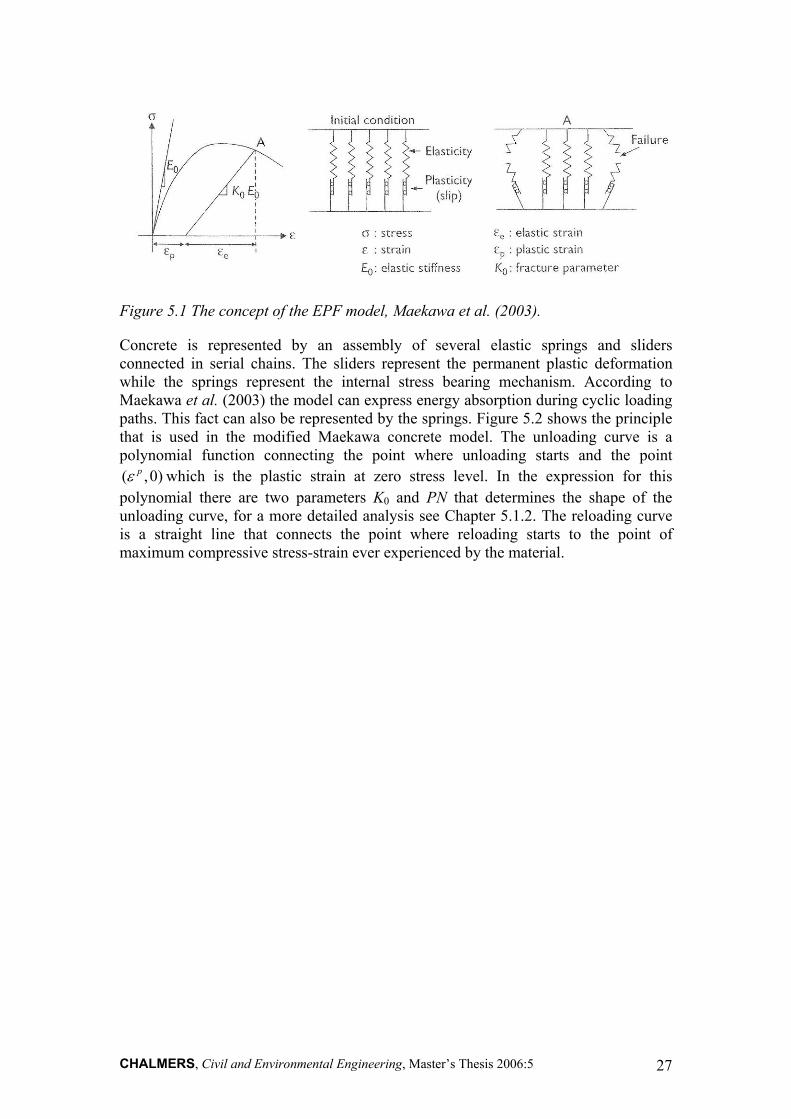
Figure 5.1 The concept of the EPF model, Maekawa et al. (2003).
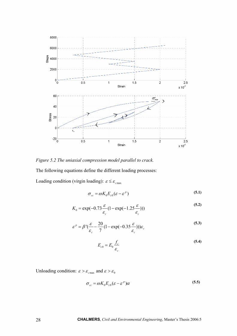
Concrete is represented by an assembly of several elastic springs and sliders connected in serial chains. The sliders represent the permanent plastic deformation while the springs represent the internal stress bearing mechanism. According to Maekawa et al. (2003) the model can express energy absorption during cyclic loading paths. This fact can also be represented by the springs. Figure 5.2 shows the principle that is used in the modified Maekawa concrete model. The unloading curve is a polynomial function connecting the point where unloading starts and the point ( ,0)pε which is the plastic strain at zero stress level. In the expression for this polynomial there are two parameters K0 and PN that determines the shape of the unloading curve, for a more detailed analysis see Chapter 5.1.2. The reloading curve is a straight line that connects the point where reloading starts to the point of maximum compressive stress-strain ever experienced by the material.
CHALMERS, Civil and Environmental Engineering, Master’s Thesis 2006:5 28
Figure 5.2 The uniaxial compression model parallel to crack.
The following equations define the different loading processes:
Loading condition (virgin loading): maxcε ε≤
0 0 ( )pcc cK Eσ ω ε ε= − (5.1)
0 exp( 0.73 (1 exp( 1.25 )))c c
K ε εε ε
= − − − (5.2)
20'( (1 exp( 0.35 )))7
pc
c c
ε εε β εε ε
= − − − (5.3)
0 0c
cc
fE Eε
= (5.4)
Unloading condition: max 0and cε ε ε ε> >
0 0 ( )pcc cK Eσ ω ε ε α= − (5.5)
CHALMERS, Civil and Environmental Engineering, Master’s Thesis 2006:5 29
0
0 0 0 0
( )( )( )
pPNcc
p pc
slop slopK E
σ ε εαε ε ε ε
−= + −
− −
(5.6)
Reloading condition: max 0and cε ε ε ε> ≤
maxmax max 0
max 0
( ( ) )ccc c c cc
c
ε εσ ω σ σ σε ε
−= − −
−
(5.7)
In the above equation the following parameters are used:
0
0
0
0
: concrete compressive stress: current strain
: strain: fracture parameter: initial stiffness
: coefficient = 2.0c
KEE
σεε
cmax
max
0
20
: maximum compressive stress: maximum compressive strain
: current compressive stress: strength reduction factor
due to orthogonal tensile strain : unloading parameter =
:
c
cc
slop KPN
σεσω
unloading parameter = 2: uniaxial compressive strength < 0: uniaxial strain at ' : strain-rate factor = 1
c
c c
ffε
β
The difference between strain ε and current strain 0ε in terms of numerical incremental analysis is that the current strain 0ε corresponds to the actual step for which the current stress 0ccσ is searched, while the strain ε is the strain that already exists in the previous incremental step. In the following analyses it is assumed that cε is equal 0.002 and cf is equal to 50 MPa, i.e. the analyses are made for data corresponding to concrete C50. The value of cε is chosen according to CEB (1993). It must be pointed out that this value can differ depending on concrete type.
CHALMERS, Civil and Environmental Engineering, Master’s Thesis 2006:5 30
5.1.2 Analysis of parameters
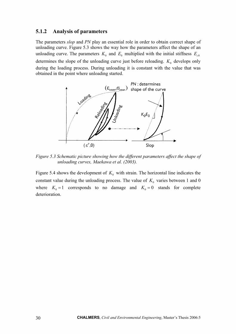
The parameters slop and PN play an essential role in order to obtain correct shape of unloading curve. Figure 5.3 shows the way how the parameters affect the shape of an unloading curve. The parameters 0K and 0E multiplied with the initial stiffness 0cE determines the slope of the unloading curve just before reloading. 0K develops only during the loading process. During unloading it is constant with the value that was obtained in the point where unloading started.
Figure 5.3 Schematic picture showing how the different parameters affect the shape of unloading curves, Maekawa et al. (2003).
Figure 5.4 shows the development of 0K with strain. The horizontal line indicates the constant value during the unloading process. The value of 0K varies between 1 and 0 where 0 1K = corresponds to no damage and 0 0K = stands for complete deterioration.

CHALMERS, Civil and Environmental Engineering, Master’s Thesis 2006:5 31
Figure 5.4 Development of the parameter K0. The upper part of the diagram shows the corresponding stress-strain relation.
In case of static loading a curve that is shown in Figure 5.5 was obtained. As can seen the shape of the static loading stress-strain curve resembles the theoretical curves that can be find in the literature, e.g. CEB (1993). Figure 5.6 shows how the K0 parameter develops from 1 to zero together with total strain. It is clear that the parameter obtains zero value when the stresses are zero. It follows also from Equation (5.1).
Figure 5.5 Stress strain relation in case of static loading.

CHALMERS, Civil and Environmental Engineering, Master’s Thesis 2006:5 32
Figure 5.6 Comparison between the development of stress-strain relation and the development of K0. The upper part of the figure shows the same stress-strain development as in Figure 5.5 for static loading. The lower part shows the simultaneous development of the fracture parameter K0.
As stated earlier the parameter PN decides about the curvature of the unloading curve. Figure 5.7 shows how different values of the parameter PN change the curvature. The parameter PN is originally proposed by Maekawa et al. (2003) to be equal to 2 but as shown in Figure 5.7, it is possible to modify the curvature if such a modification would be required. Independent of which PN value is chosen, the value of plastic strain, pε , corresponding to the maximum compressive stress maxcσ , will be the same.

CHALMERS, Civil and Environmental Engineering, Master’s Thesis 2006:5 33
Figure 5.7 Unloading curves for different values of the parameter PN.
In the same way as K0, the plastic strain pε develops only when the current strain exhibits the maximal strain value maxcε i.e. when the current point in the stress-strain space is lying on the virgin loading curve. Lower part of Figure 5.8 shows stress-strain relation for a strain input that is shown in the upper part of the figure.
Figure 5.8 Strain input and stress-strain diagram for the case with many unloading and reloading curves.
PN=1
PN=2
PN=3
PN=4

CHALMERS, Civil and Environmental Engineering, Master’s Thesis 2006:5 34
Figure 5.9 shows the development of plastic strain, pε , for corresponding stress-strain diagram. As in case with K0, the horizontal lines correspond to the unloading and reloading curves (cf. Figure 5.8) where pε is constant.
Figure 5.9 Plastic strain development as function of total strain.
As can be concluded from the analysis of both figures, different plastic strains will be obtained dependent on where the unloading to zero stress level occurs. These plastic strains can be found on the plastic strain versus total strain diagram in Figure 5.9.
5.1.3 Stresses development due to constant amplitude cyclic loading
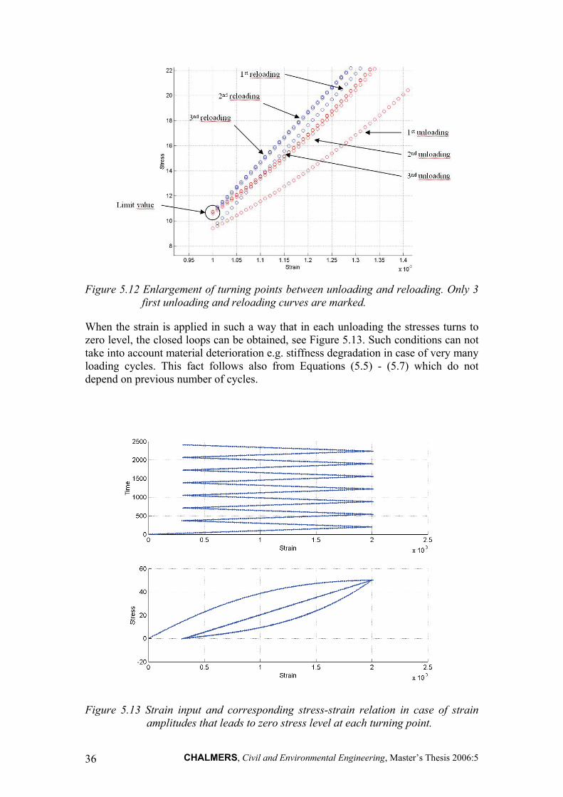
In order to check how constant amplitude cyclic loading influences the stress-strain relationship of the modified Maekawa concrete model, the strains were applied according to the upper part of Figure 5.10. The lower part of the Figure 5.10 shows the corresponding stress-strain relation ship. From the simulations one can see that if the unloading curves do not turn to zero stress level the stresses obtained for the following unloading curves will increase little at the turning point between the unloading and reloading curve. This increase has a limit value which is obtained already after one or two reloadings. Thus, the model represents cyclic hardening. This fact is presented in Figure 5.11 and Figure 5.12.

CHALMERS, Civil and Environmental Engineering, Master’s Thesis 2006:5 35
Figure 5.10 Strains versus time and stress-strain relationship in case of constant amplitude cyclic loading.
Figure 5.11 Stress-strain relation obtained for the strains presented in Figure 5.10.
CHALMERS, Civil and Environmental Engineering, Master’s Thesis 2006:5 36
Figure 5.12 Enlargement of turning points between unloading and reloading. Only 3 first unloading and reloading curves are marked.
When the strain is applied in such a way that in each unloading the stresses turns to zero level, the closed loops can be obtained, see Figure 5.13. Such conditions can not take into account material deterioration e.g. stiffness degradation in case of very many loading cycles. This fact follows also from Equations (5.5) - (5.7) which do not depend on previous number of cycles.
Figure 5.13 Strain input and corresponding stress-strain relation in case of strain amplitudes that leads to zero stress level at each turning point.
CHALMERS, Civil and Environmental Engineering, Master’s Thesis 2006:5 37
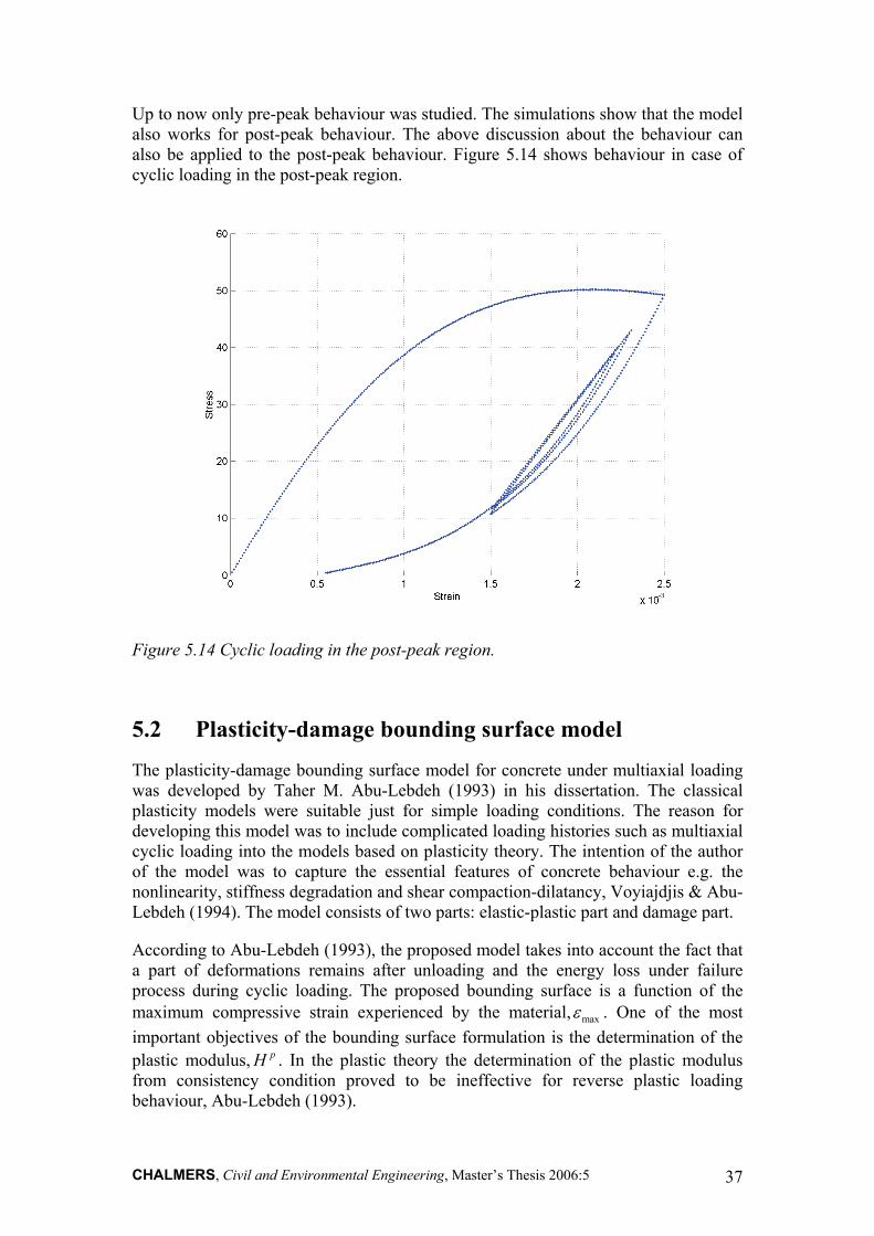
Up to now only pre-peak behaviour was studied. The simulations show that the model also works for post-peak behaviour. The above discussion about the behaviour can also be applied to the post-peak behaviour. Figure 5.14 shows behaviour in case of cyclic loading in the post-peak region.
Figure 5.14 Cyclic loading in the post-peak region.
5.2 Plasticity-damage bounding surface model
The plasticity-damage bounding surface model for concrete under multiaxial loading was developed by Taher M. Abu-Lebdeh (1993) in his dissertation. The classical plasticity models were suitable just for simple loading conditions. The reason for developing this model was to include complicated loading histories such as multiaxial cyclic loading into the models based on plasticity theory. The intention of the author of the model was to capture the essential features of concrete behaviour e.g. the nonlinearity, stiffness degradation and shear compaction-dilatancy, Voyiajdjis & Abu-Lebdeh (1994). The model consists of two parts: elastic-plastic part and damage part.
According to Abu-Lebdeh (1993), the proposed model takes into account the fact that a part of deformations remains after unloading and the energy loss under failure process during cyclic loading. The proposed bounding surface is a function of the maximum compressive strain experienced by the material, maxε . One of the most important objectives of the bounding surface formulation is the determination of the plastic modulus, pH . In the plastic theory the determination of the plastic modulus from consistency condition proved to be ineffective for reverse plastic loading behaviour, Abu-Lebdeh (1993).
CHALMERS, Civil and Environmental Engineering, Master’s Thesis 2006:5 38
5.2.1 Constitutive equations
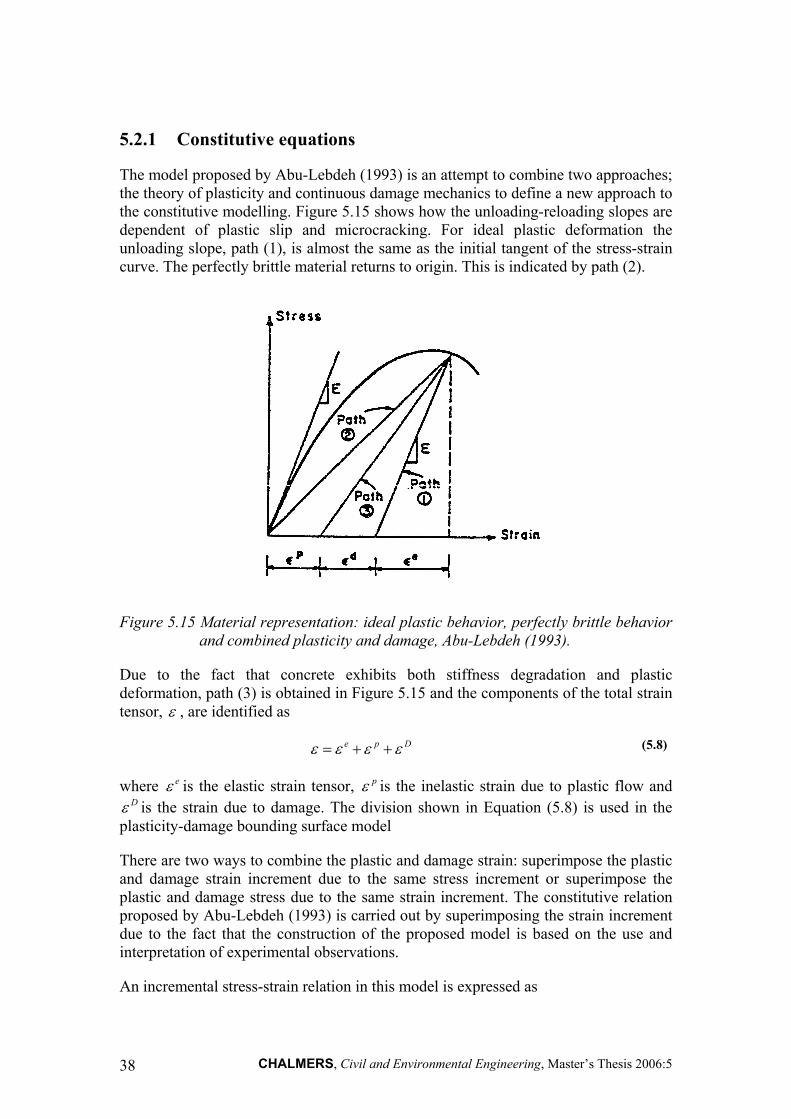
The model proposed by Abu-Lebdeh (1993) is an attempt to combine two approaches; the theory of plasticity and continuous damage mechanics to define a new approach to the constitutive modelling. Figure 5.15 shows how the unloading-reloading slopes are dependent of plastic slip and microcracking. For ideal plastic deformation the unloading slope, path (1), is almost the same as the initial tangent of the stress-strain curve. The perfectly brittle material returns to origin. This is indicated by path (2).
Figure 5.15 Material representation: ideal plastic behavior, perfectly brittle behavior and combined plasticity and damage, Abu-Lebdeh (1993).
Due to the fact that concrete exhibits both stiffness degradation and plastic deformation, path (3) is obtained in Figure 5.15 and the components of the total strain tensor, ε , are identified as
e p Dε ε ε ε= + + (5.8)
where eε is the elastic strain tensor, pε is the inelastic strain due to plastic flow and Dε is the strain due to damage. The division shown in Equation (5.8) is used in the
plasticity-damage bounding surface model
There are two ways to combine the plastic and damage strain: superimpose the plastic and damage strain increment due to the same stress increment or superimpose the plastic and damage stress due to the same strain increment. The constitutive relation proposed by Abu-Lebdeh (1993) is carried out by superimposing the strain increment due to the fact that the construction of the proposed model is based on the use and interpretation of experimental observations.
An incremental stress-strain relation in this model is expressed as

CHALMERS, Civil and Environmental Engineering, Master’s Thesis 2006:5 39
0 0
1 13 3 9 3
( )
ij ijmnij ij mn ij mme p e
t
I II I IIijkl ijkl kl ijkl kl ijkl kl
d SSd d dH H K H
C C d dC dC
σ βε δ σ δ στ τ
σ σ σ+ −
⎛ ⎞ ⎛ ⎞= + + + −⎜ ⎟ ⎜ ⎟
⎝ ⎠ ⎝ ⎠+ + + +
(5.9)
where
0
, : stress tensor and its increment
, : generalized elastic and plastic shear modulia : deviatoric stress tensor
: octahedral shear stress: shear compaction-dilatancy factor
: tangent bulk mo
ij ij
e p
ij
t
d
H HS
K
σ σ
τβ
+
dulus
, : compliance tensors corresponding to tensile and compressive stresses, : positive (tensile), and negative (compression) stresses
I IIC Cσ σ −
Elasto-plastic part of the model
In Equation (5.9) the first three terms corresponds to plastic and elastic strain, compare with Equation (5.8), i.e.:
0 0
1 13 3 9 3
ij ijp e mnij mn ij mme p e
t
d SSd d d dH H K Hσ βε ε δ σ δ σ
τ τ⎛ ⎞ ⎛ ⎞
+ = + + + −⎜ ⎟ ⎜ ⎟⎝ ⎠ ⎝ ⎠
(5.10)
From Equation (5.10), it is clear that the parameters of the proposed plasticity model are the elastic shear modulus, eH , the plastic shear modulus, pH , the bulk tangent modulus, tk , and the shear compaction-dilatancy factor, β .
Elastic shear modulus
The generalized elastic shear modulus, eH , is assumed as the initial slope of the shear stress-strain curve, and is determined for both deviatoric loading and unloading as shown below:
21
e EH Gv
= =+
(5.11)
Where, G , is the shear modulus of elasticity, E , is the Young’s modulus, and, v ,is the Poisson’s ratio.
Plastic shear modulus
The plastic shear modulus, pH , depends on the current stress, ijσ , the maximum principal compressive strain experienced by the material, maxε , and on the normalized distance, d, between the current stress point and the bounding surface. The bounding

CHALMERS, Civil and Environmental Engineering, Master’s Thesis 2006:5 40
surface as well as the normalized distance, d, is described in detail in Chapter 5.2.2. The following equations determine the plastic modulus:
1. For monotonic (virgin) loading:
121
121
20 for 3.0( 0.5)
3.0 for 3.0( 1.45)
p c
p c
H fH II
H fH II
= ≥ −−
−= < −
+
(5.12)
Where 0.52 0.2
max
( ) (1.1 cos3 )H dδ θε
⎛ ⎞= +⎜ ⎟⎜ ⎟⎝ ⎠
. Stresses are normalized with respect to the
compressive strength cf . The function 3/ 23 2cos3 3 3 / 2J Jθ = comes from the
definition of bounding surface proposed by Ottosen (1977) and δ is the value of the distance of current stress point from the bounding surface at beginning of current loading process. In the above equations 1 2 3, and I J J are the first, second and third stress invariant, respectively.
2. For unloading:
0.52
0.65 0.351 max
1.35( )( )
p cd fHH ε δ
= (5.13)
in which
21,max 1,max 1
1 10.4
11,max
1,max1 10.4
( 0.5) 1.176( 0.5)( 0.5)for 3.0
14(1.1 cos3 )0.5( 1.45)(1.16 1)
0.5for 3.0
1.77(1.1 cos3 )
I I IH I
III
H I
θ
θ
− − − −= ≥ −
+−
− −−
= < −+
where 1,maxI is the maximum value of 1I before the current unloading.
3. For reloading
max150
2
350 (10)pc
dH fH
εδ −= (5.14)
where

CHALMERS, Civil and Environmental Engineering, Master’s Thesis 2006:5 41
21
2 10.2
21
2 10.2
( 0.5) for 3.010(1.1 cos3 )
0.82( 1.45) for 3.0(1.1 cos3 )
IH I
IH I
θ
θ
−= ≥ −
+
− += < −
+
The above definitions of plastic shear modulus are determined by fitting the available monotonic and cyclic experimental data. Based on these data, it was observed that the tangent modulus decreases gradually to zero as the stress point approaches the bounding surface (for discussion on failure surface see Chapter 5.2.3). This fact follows also from examination of Equations (5.11), (5.12) and (5.13).
Bulk tangent modulus
The bulk tangent modulus, tk , is found as:
01.35
1
0
1.25 in case of hydrostatic loading1 0.4( )1.15 in case of hydrostatic unloading
t
t
kkI
k k
=+ −
=
(5.15)
where 0k is the initial value of tk which is equal to 500 cf . The bulk tangent modulus relates the hydrostatic stress with the corresponding volume strain.
Compaction-dilatancy factor
The coupling between volumetric and deviatoric component is generally defined as shear compaction-dilatancy effect. The effect originates in the fact that the volumetric strain is caused by both volumetric stress and deviatoric stress, i.e. octahedral shear. This effect is considered by the shear compaction-dilatancy factor β :
0.23max10.25( ) ( 0.2)dβ ε= − (5.16)
Damage part of the model
In Equation (5.9) the last three terms describe the increase of strain due to damage, e.i.
( )D I II I IIijkl ijkl kl ijkl kl ijkl kld C C d dC dCε σ σ σ+ −= + + + (5.17)
In the above equation I and II refer to mode I and II of cracking, respectively. The two modes describe two different cracking effects and are defined by Abu-Lebdeh (1993) as follows: mode I represents cleavage cracking and mode II represents sliding of two planes. These modes are presented in Figure 5.16.

CHALMERS, Civil and Environmental Engineering, Master’s Thesis 2006:5 42
Figure 5.16 Schematic representaion of modes I and II type of failure, Abu-Lebdeh (1993).
According to Abu-Lebdeh (1993) the first term in the Equation (5.17) represents the rate of elastic deformation for uncracked material, while the last two terms represent the rate of deformation due to the elastic damage. Equation (5.17) shows that cleavage cracking is due to the positive stress tensor, σ + , which is obtained by removing the stress tensor associated with negative eigenvalues from the total stress tensor, Abu-Lebdeh (1993). The compressive mode of cracking is produced by the negative cone of the stress tensor, σ − , which is obtained by removing the positive eigensystem from the total stress σ . The following matrices define the compliance tensors for tensile and compressive stresses, respectively:
11
0 22
33
1(1 )
1 1(1 )
1(1 )
I
v vD
C v vE D
v vD
γ
γ
γ
⎡ ⎤− −⎢ ⎥−⎢ ⎥
⎢ ⎥= − −⎢ ⎥−⎢ ⎥
⎢ ⎥− −⎢ ⎥
−⎣ ⎦
(5.18)
22 33 11 22 11 33
0 11 22 11 33 22 33
11 33 22 33 11 22
1(1 )(1 ) (1 )(1 ) (1 )(1 )
1 1(1 )(1 ) (1 )(1 ) (1 )(1 )
1(1 )(1 ) (1 )(1 ) (1 )(1 )
d d
II
d d
d d
v vD D D D D D
v vCE D D D D D D
v vD D D D D D
β β
β β
β β
⎡ ⎤− −⎢ ⎥− − − − − −⎢ ⎥⎢ ⎥− −
= ⎢ ⎥− − − − − −⎢ ⎥⎢ ⎥− −⎢ ⎥
− − − − − −⎣ ⎦
(5.19)
In the above definitions of the compliance matrices 0E and v is the modulus of elasticity and the Poisson’s ratio, respectively. 11 22 33, and D D D are the accumulated damage components in planes perpendicular to the principal axis. These damage

CHALMERS, Civil and Environmental Engineering, Master’s Thesis 2006:5 43
components are discussed more in detail in Chapter 5.2.3. The parameter γ accounts for the crack geometry on the stress intensity of concrete in tension and is chosen to be equal to 4, based on experimental data. In the same way the parameter dβ accounts for the crack growth in compression, and is selected to be equal to 0.1. The rate compliance matrices IdC and IIdC are derived by taking the partial derivative with respect to the accumulated damage components 11 22 33, and D D D , on the components of the compliance matrices defined in Equations (5.18) and (5.19).
5.2.2 Bounding surface concept The concept introduces a bounding surface which is identical to that of a yield surface in the classical theory of plasticity. The surface encloses all the subsequent loading surfaces in stress space. It may deform and translate in stress space if plastic loading takes place. Due to the fact that concrete is hydrostatic-pressure dependent material the bounding surface has curved meridians, Chen & Han (1988). This fact is supported by experimental works of Ottosen (1977) among others. The results of these experiments show clearly that the bounding surface is curved, smooth, convex and depends on the angle of similarity θ.
Failure of materials is usually defined in terms of its load-carrying capacity. In case of brittle materials, such as concrete, and in contrast to ductile materials, such as steel, the behaviour is characterized by its hydrostatic pressure dependence. It means that the stress invariants should not be omitted in the definition of a bounding surface. According to the above the general form describing a bounding surface can be formulated as follows:
0),,( 321 =JJIf or 0),,( =θρξf (5.20)
where I1, J2 and J3 are the first, second and third stress invariant respectively, ξ is a value on the hydrostatic axis, ρ is a vector in plane with the deviatoric plane and θ is the angle of similarity defined in Figure 5.18.
Figure 5.17 a) Concrete failure surface in 3D-stress state, Strauss et al. (2003). b) Failure surface on meridians and c) on deviatoric plane, Voyiajdjis & Abu-Lebdeh (1994).
a) b) c)

CHALMERS, Civil and Environmental Engineering, Master’s Thesis 2006:5 44
The explicit form of the equations above is defined from experimental data. The meridians start at a point of hydrostatic tensile strength and open in the direction of the negative hydrostatic pressure, as has been showed in Figure 5.17. The curvature of the meridians indicates that the shearing capacity (in Figure 5.17a defined by τ0) is increasing with increasing hydrostatic pressure.
It should be pointed that according to this description of a bounding surface a pure hydrostatic loading can not cause failure. A failure curve along the compressive meridian up to I1=-79fc has been determined experimentally by Chinn & Zimmerman (1965) without observing any tendency to approach the hydrostatic axis.
The cross-section of the bounding surface, when presented on deviatoric plane, has a threefold symmetry and 120º period. This fact is motivated by the isotropy of the material, Chen & Han (1988). Due to this fact the experiments with multiaxial loading needs to be performed on the interval θ=0º to θ=60º, where θ is often called the angle of similarity in the technical literature. States of stresses as well as strengths within other sectors will be known by symmetry. The meridian that corresponds to the angle of similarity, θ=60º, describes a hydrostatic state of stresses with a compressive stress superimposed in one direction. Thus, this state reminds highly about a typical compression test and the corresponding meridian is called consequently the compression meridian. In similar way the meridian which is determined by, θ=0º, is called the tension meridian due to the fact that it describes a situation that is comparable with a tension test where a tensile stress is superimposed in one direction. This is showed in Figure 5.18. The meridian determined by θ=30º is occasionally called the shear meridian.
Figure 5.18 Basic features of bounding surface a) meridians b) deviatoric plane.
The first attempt to generalize the conventional flow theory to include the hysteretic behaviour of metals is the model proposed by Dafalias & Popov (1975), Dafalias & Popov (1976), Dafalias & Popov (1977) and independently by Krieg (1975). The concept was first applied to concrete by Fardis et al. (1983).
With the purpose of study if failure occurs in the material it is usually needed to check whether the stress point lies inside or on the loading surface. This is the common way of many algorithms. The idea with introduction of the concept of the bounding surface is that it uses the distance δ between the present stress point which is within the bounding surface and the corresponding image point on the bounding surface, see Figure 5.17 b). In such a way it is possible to vary the plastic shear modulus with respect to the distance that is separating the stress point from the current failure. By current failure it is meant an image point on the bounding that corresponds to the failure if the loads would increase statically in the direction of this image point.
σ1
σ2 σ3
angle θ θ=60º
θ=0º
I1
ρ a) b)

CHALMERS, Civil and Environmental Engineering, Master’s Thesis 2006:5 45
The key of the plasticity bounding surface model suggested by Abu-Lebdeh (1993) is that it is a modification of the monotonic failure surface proposed by Ottosen (1977) so that it becomes a function of the strain history. The bounding surface function in the present model is given in the form:
max max 2 2 1( , ) [ 0.52 (2.53 ln )] 1 0ijF A B J J BIσ ε ε λ= + − − + + − = (5.21)
where maxε is the maximum principal compressive strain experience in the material, A and B are constants given by Ottosen (1977) and λ is a function of cos(3 )θ , that is also given by Ottosen (1977). In this model the author decided to define the distance δ to be measured on the deviatoric plane, according to Figure 5.17 c). It should be noted that the stress invariants appearing in the bounding surface criterion, Eq. (5.21), are normalized by the uniaxial compressive strength cf , e.g. 1I and 2J represent
1 / cI f and 22 / cJ f , respectively.
5.2.3 Continuum damage mechanics
Continuum damage mechanics assumes that the failure starts in an uncracked material due to a gradual deterioration of a continuously deforming material. This vision is suited best for material that behaves in a ductile fashion. Due to ductility stress drops rather spectacularly and deformations concentrate in a narrow zone. The idea behind the calculation of stresses in damage mechanics is to introduce a damage variable, nD , that, when multiplying with a fictitious undamaged stress called effective, obtains a nominal stress which is actually prevailing in a damaged material.
The damage variable is usually a mathematic function that varies between a value a and another value b (can be a scalar, vector or tensor), where a≠b. Then it is possible to state that there is no damage when nD a= and total damage when 0nD b− → . In order to exemplify the above discussion in terms of mathematical expressions, it is possible to use the definitions of the damage variable as originally proposed by Kachanov (1958) and reviewed by Kattan & Voyiadjis (2002):
'n
A ADA−
= (5.22)
Where, A’, is the cross-sectional area of the undamaged, original, material specimen and, A, is the (effective) area of the damaged, actual, material specimen. Thus, it is clear that 0 1nD< < characterizes the damage state. According to Kattan & Voyiadjis (2002) the nominal stress can be obtained by using the damage variable in the following way:
'1 nDσσ =−
(5.23)
Where, σ’, is the nominal stress and, σ, is the effective stress. In this case it can be observed that the current stress will turn to zero for the totally damaged material,

CHALMERS, Civil and Environmental Engineering, Master’s Thesis 2006:5 46
which is in accordance with the physical laws. The above discussion is also presented illustratively in Figure 5.19, on a cylindrical bar subjected to a uniaxial tension by a force T.
Figure 5.19 A cylindrical bar subjected to uniaxial tension, Kattan & Voyiadjis (2002).
Damage modelling in the proposed model
From the perspective of constitutive modelling the above way of defining the damage variable, i.e. with help of different areas, is not effective, as was already discussed in Chapter 4.2. This is due to the fact that the evolution of damage is essentially anisotropic. Thus, it is not possible to describe damage with one single damage parameter. As was already stated in Chapter 4.2 three damage variables are used in the present model. In order to describe the rate compliance matrices IdC and IIdC , it is needed to define the damage growth rate. This can be done by using the continuum damage mechanics. In the present model, a continuum damage theory for cyclic loading is formulated using a concept similar to the plasticity bounding surface. The damage growth rate is derived using the concept of damage bounding surface which introduces a bounding surface, a loading surface and an initial fracture surface.
The following equations describe these three surfaces:
Damage bounding surface
2 2 125.7( , ) 0
27ijF D aJ J bID
σ λ= + + − =+
(5.24)
where a and b are constants, λ is a function of cos3θ given by Ottosen (1977), and D is the maximum value of damage accumulation ever experienced by the material.
Loading surface
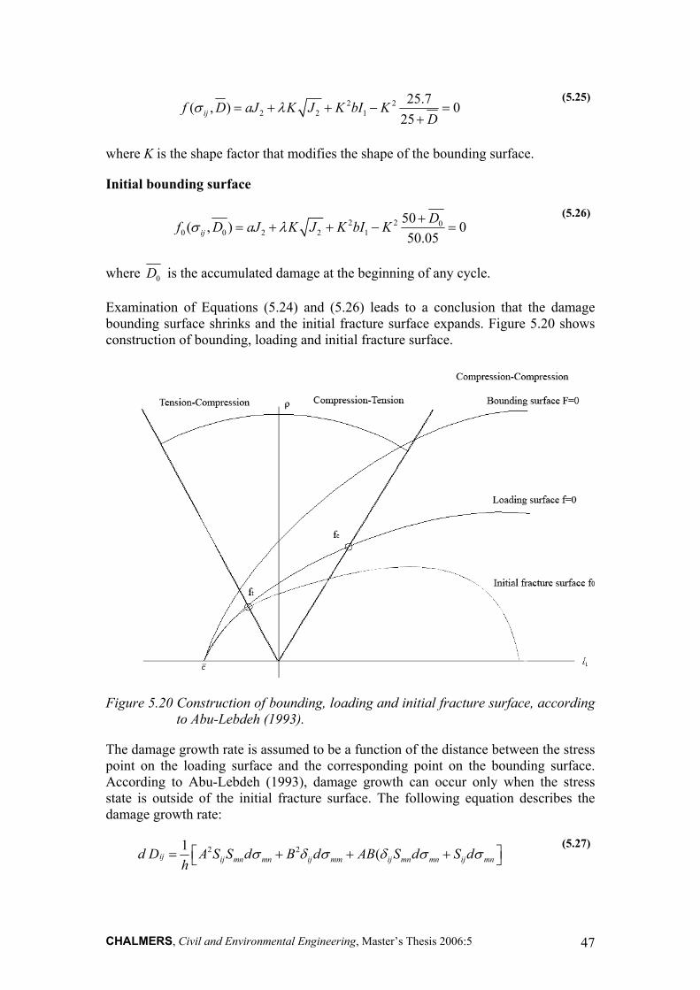
CHALMERS, Civil and Environmental Engineering, Master’s Thesis 2006:5 47
2 22 2 1
25.7( , ) 025ijf D aJ K J K bI K
Dσ λ= + + − =
+
(5.25)
where K is the shape factor that modifies the shape of the bounding surface.
Initial bounding surface
2 2 00 0 2 2 1
50( , ) 050.05ij
Df D aJ K J K bI Kσ λ += + + − =
(5.26)
where 0D is the accumulated damage at the beginning of any cycle.
Examination of Equations (5.24) and (5.26) leads to a conclusion that the damage bounding surface shrinks and the initial fracture surface expands. Figure 5.20 shows construction of bounding, loading and initial fracture surface.
Figure 5.20 Construction of bounding, loading and initial fracture surface, according to Abu-Lebdeh (1993).
The damage growth rate is assumed to be a function of the distance between the stress point on the loading surface and the corresponding point on the bounding surface. According to Abu-Lebdeh (1993), damage growth can occur only when the stress state is outside of the initial fracture surface. The following equation describes the damage growth rate:
2 21 (ij ij mn mn ij mm ij mn mn ij mnd D A S S d B d AB S d S dh
σ δ σ δ σ σ⎡ ⎤= + + +⎣ ⎦ (5.27)
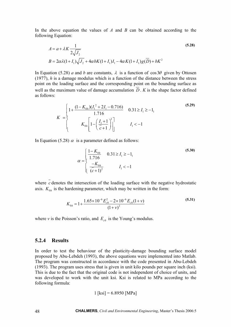
CHALMERS, Civil and Environmental Engineering, Master’s Thesis 2006:5 48
In the above equation the values of A and B can be obtained according to the following Equation:
2
21 2 1 1 1
12
2 (1 ) 4 (1 ) 4 (1 ) ( )
A a KJ
B I J bK I I K I g D bK
λ
αλ α α
= +
= + + + − + +
(5.28)
In Equation (5.28) a and b are constants, λ is a function of cos3θ given by Ottosen (1977), h is a damage modulus which is a function of the distance between the stress point on the loading surface and the corresponding point on the bounding surface as well as the maximum value of damage accumulation D . K is the shape factor defined as follows:
20 1 1
1 1
21
0 1
(1 )( 2 0.716)1 0.31 11.716
11 11
h
h
K I I I
KIK Ic
⎧ − + −+ ≥ ≥ −⎪
⎪= ⎨ ⎡ ⎤+⎛ ⎞⎪ − < −⎢ ⎥⎜ ⎟⎪ +⎝ ⎠⎢ ⎥⎣ ⎦⎩
(5.29)
In Equation (5.28) α is a parameter defined as follows:
01 1
012
1 0.31 11.716
1( 1)
h
h
K I
K Ic
α
−⎧ ≥ ≥ −⎪⎪= ⎨ −⎪ < −⎪ +⎩
(5.30)
where c denotes the intersection of the loading surface with the negative hydrostatic axis. 0hK is the hardening parameter, which may be written in the form:
6 2 6
0 00 2
1.65 10 2 10 (1 )1(1 )
c ch
E E vKv
− −× − × += +
+
(5.31)
where v is the Poisson’s ratio, and 0cE is the Young’s modulus.
5.2.4 Results
In order to test the behaviour of the plasticity-damage bounding surface model proposed by Abu-Lebdeh (1993), the above equations were implemented into Matlab. The program was constructed in accordance with the code presented in Abu-Lebdeh (1993). The program uses stress that is given in unit kilo pounds per square inch (ksi). This is due to the fact that the original code is not independent of choice of units, and was developed to work with the unit ksi. Ksi is related to MPa according to the following formula:
1 [ksi] = 6.8950 [MPa]

CHALMERS, Civil and Environmental Engineering, Master’s Thesis 2006:5 49
In the most simulations presented below, the data for concrete C50 was used. This corresponds to the following constants:
50 MPa = 7.2516 ksiE = 39 GPa = 5656.3 ksi
cf =
Figure 5.21 shows the stress-strain response of the model in case of cyclic loading; presented in Figure 5.22. Visual investigation of the cyclic behaviour presented in Figure 5.21 results in a conclusion that the model gives a reasonable picture of some of the typical details that follow the cyclic loading of concrete. These are energy loss due to repeated loadings and unloadings as well as the stiffness degradation, even if the degradation is small. Energy loss can be seen by examination of Figure 5.23, which shows the monotonic, uniaxial loading together with the cyclic loading curve. It can be seen that the envelope of the cyclic loading curve is less than the monotonic loading curve, especially after many loading cycles. It means that a larger strain is produced for the same stress level in case of cyclic loading. It follows that the material loses its energy in every reloading cycle.
Figure 5.21 Stress-strain curve in case of uniaxial, compressive cyclic loading.
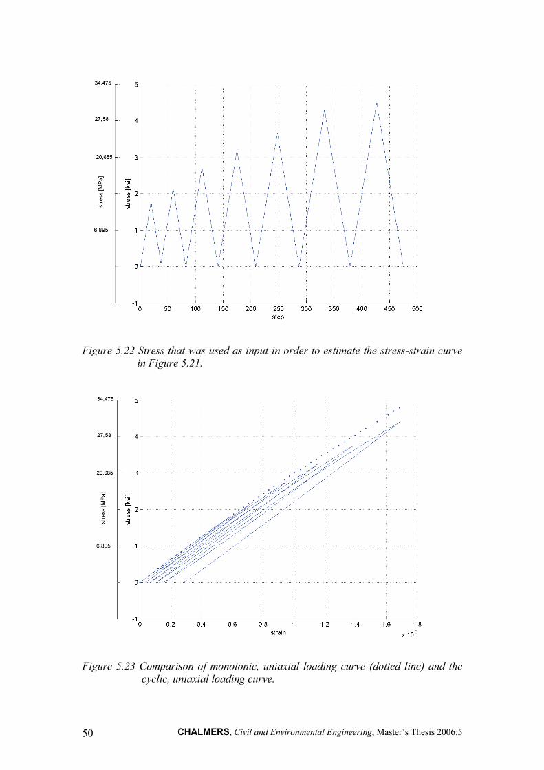
CHALMERS, Civil and Environmental Engineering, Master’s Thesis 2006:5 50
Figure 5.22 Stress that was used as input in order to estimate the stress-strain curve in Figure 5.21.
Figure 5.23 Comparison of monotonic, uniaxial loading curve (dotted line) and the cyclic, uniaxial loading curve.

CHALMERS, Civil and Environmental Engineering, Master’s Thesis 2006:5 51
Figure 5.24 shows the stress-strain curve developed for cyclic loading up to 30.4 10ε −= ⋅ followed by monotonic loading up to 110% of cf . As can be seen the
curve does not intend to straighten in order to become horizontal in the neighbourhood of the compression capacity cf . This is clearly a disadvantage of the model. In fact neither the cyclic loading curves nor the monotonic loading curves can obtain this behaviour, independently of uniaxial, biaxial or triaxial loading. The monotonically increasing performance of the stress-strain curve is valid even if the limit of the compression capacity is passed with a large amount of stress, i.e. the curve will never produce a derivative that is equal to zero. This fact is motivated by the construction of the algorithm. The algorithm can not distinguish if the stress vector describe the falling branch of the monotonic stress-strain curve or if the stress vector describes the unloading. This motivation is explained in Figure 5.25. As can be seen the stress vector is constructed exactly in the same way both in the case of loading-unloading and in the monotonic loading-to-failure case. A correctly working algorithm must then recognize which case is correct for the specific situation. The model is not able to do this and recognizes such behaviour only as unloading.
Figure 5.24 Cyclic loading followed by monotonicaly increasing loading up to 110% of the compression capacity.

CHALMERS, Civil and Environmental Engineering, Master’s Thesis 2006:5 52
Figure 5.25 The reason to the fact that the algorithm can not recognize if the loading-unloading or the monotonic loading-to-failure is current. The dashed arrow shows how the algorithm actually recognizes the monotonic loading-to-failure.
As mentioned before the total strain is composed of the strain due to elastic and plastic response as well as the strain due to damage, cf. Equation (5.8). Figure 5.26 shows the different strains. As can be concluded, the development of the strain due to damage is almost independent of number of cycles. This is indicated by a unique, linear behaviour of the damage strain. It means that the shape of the total strain curve rests on the elastic-plastic part of the total strain. Another interesting thing can be found when examining a region near origin in Figure 5.27. The region is shown in Figure 5.28. It can be concluded that the damage part of the total strain becomes negative with number of cycles.
σ
ε
Vector describing loading and then unloading
σ = [a b c d c b a] where a<b<c<d
Algorithm
Result
σ
ε
Vector describing monotonic loading-to-failure
σ = [a b c d c b a] where a<b<c<d
Algorithm
Result
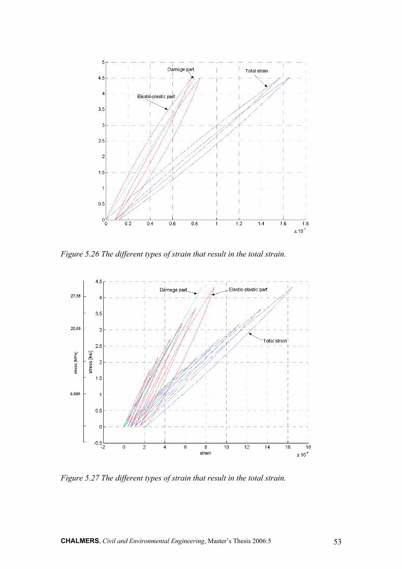
CHALMERS, Civil and Environmental Engineering, Master’s Thesis 2006:5 53
Figure 5.26 The different types of strain that result in the total strain.
Figure 5.27 The different types of strain that result in the total strain.

CHALMERS, Civil and Environmental Engineering, Master’s Thesis 2006:5 54
Figure 5.28 The region near origin of the stress-strain curve showed in the previous figure.
According to Abu-Lebdeh (1993), in particular case of a test that is called cyclic stress reversal test, a remaining stress can be obtained when strain is zero. The Matlab code, which is based on the code proposed by Abu-Lebdeh (1993) also gives a similar result. The result is obtained when the stress that is used as input in the code grow to a certain value and then unloading is initiated. Figure 5.29 shows a sequence of six pictures. In each picture the maximum stress ever experienced was increased with some small value relative to the previous one. It can be seen that the last unloading curve changes from smooth to piecewise smooth in Figure 5.29 d). The last unloading curve is the developing from being non-smooth to being discontinuous. This discontinuity is especially emphasized when the maximum stress is large enough. This is shown in Figure 5.30. If the part below the point of discontinuity would be cut the result similar to the one shown in Abu-Lebdeh (1993) would be obtained. This behaviour is not trustworthy, and thus it can be regarded as a disadvantage of the model.

CHALMERS, Civil and Environmental Engineering, Master’s Thesis 2006:5 55
Figure 5.29 Sequence showing the development of point of discontinuity.
Figure 5.30 Fully developed point of discontinuity.
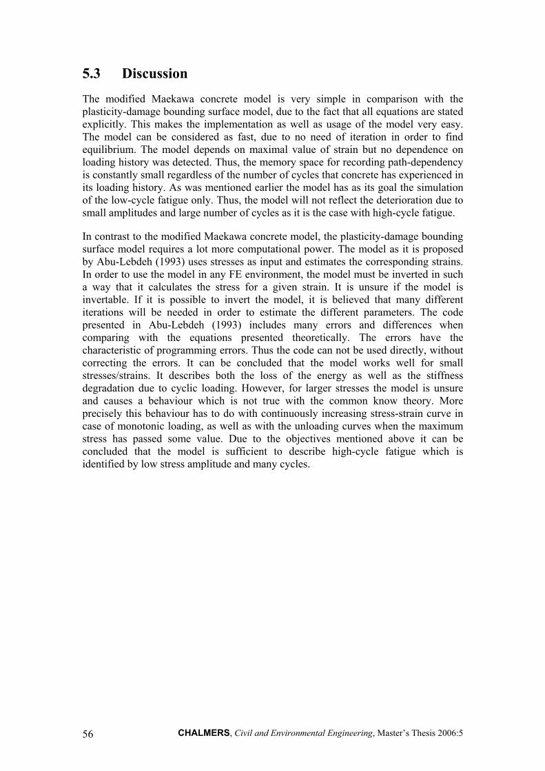
CHALMERS, Civil and Environmental Engineering, Master’s Thesis 2006:5 56
5.3 Discussion
The modified Maekawa concrete model is very simple in comparison with the plasticity-damage bounding surface model, due to the fact that all equations are stated explicitly. This makes the implementation as well as usage of the model very easy. The model can be considered as fast, due to no need of iteration in order to find equilibrium. The model depends on maximal value of strain but no dependence on loading history was detected. Thus, the memory space for recording path-dependency is constantly small regardless of the number of cycles that concrete has experienced in its loading history. As was mentioned earlier the model has as its goal the simulation of the low-cycle fatigue only. Thus, the model will not reflect the deterioration due to small amplitudes and large number of cycles as it is the case with high-cycle fatigue.
In contrast to the modified Maekawa concrete model, the plasticity-damage bounding surface model requires a lot more computational power. The model as it is proposed by Abu-Lebdeh (1993) uses stresses as input and estimates the corresponding strains. In order to use the model in any FE environment, the model must be inverted in such a way that it calculates the stress for a given strain. It is unsure if the model is invertable. If it is possible to invert the model, it is believed that many different iterations will be needed in order to estimate the different parameters. The code presented in Abu-Lebdeh (1993) includes many errors and differences when comparing with the equations presented theoretically. The errors have the characteristic of programming errors. Thus the code can not be used directly, without correcting the errors. It can be concluded that the model works well for small stresses/strains. It describes both the loss of the energy as well as the stiffness degradation due to cyclic loading. However, for larger stresses the model is unsure and causes a behaviour which is not true with the common know theory. More precisely this behaviour has to do with continuously increasing stress-strain curve in case of monotonic loading, as well as with the unloading curves when the maximum stress has passed some value. Due to the objectives mentioned above it can be concluded that the model is sufficient to describe high-cycle fatigue which is identified by low stress amplitude and many cycles.
CHALMERS, Civil and Environmental Engineering, Master’s Thesis 2006:5 57
6 Conclusions and suggestions for further studies This project has studied fatigue in plain concrete, different empirical methods that can be used in order to analyze fatigue life as well as constitutive models that are capable to model cyclic loading of concrete. The following are the conclusion of the work and suggestion for further studies.
6.1 Conclusions
• Fatigue consists of progressive, internal and permanent structural changes in the material.
• The fatigue process in concrete starts with propagation of already existing microcracks. The existence of microcracks in concrete is due to shrinkage caused by temperature variations during hardening period.
• Fracture of concrete due to cyclic loading causes problems and large economic costs. This may be connected with the fact that modern structures are slender which leads to stress concentrations. This is also connected with the fact that modern structures are often intended to cooperate with sources of cyclic loading during long time.
• The empirical methods used for analysing fatigue in concrete, origin in investigations on cyclic loading in steel.
• In order to analyse and design structures with respect to cyclic loading one needs a proper constitutive model that can be used in FE environment.
• A constitutive model should be easy to use and should not require a lot of computational power in order to be effective.
• Fatigue is a complex phenomenon that requires special constitutive models that can take into account stiffness degradation and loss of energy due to cyclic loading.
• The models described and analysed in this thesis have some important drawbacks. They work well only under specific conditions. Thus, they cannot be generalized in order to describe all different types of cyclic loading.
• A difficulty with implementation and testing of constitutive model is that they are not sufficiently detailed described in different scientific papers. Often important information is missing which makes the implementation strenuous and in some cases impossible.
6.2 Further studies
It would be very interesting to see how other constitutive models that are available work. In particular it would be interesting to search and investigate if there are models that are capable to describe both low-cycle and high-cycle fatigue as well as if the disadvantages that probably are connected with these models are of the same nature as

CHALMERS, Civil and Environmental Engineering, Master’s Thesis 2006:5 58
the disadvantages described in this work. If the disadvantages repeat in different models, then it is possible to concentrate the work on development or improvement of models so that they will be free from these disadvantages.
All such models need to be verified with experiments. Work on that kind of verification of existing models is also needed. This is especially important due to the fact that modern structures become slender and stress concentrations increase, which leads to a conclusion that the problem of fatigue will be even more important in the future.
CHALMERS, Civil and Environmental Engineering, Master’s Thesis 2006:5 59
7 References Abeles P. W., American Concrete Institute; Committee 215 Fatigue of Concrete (1974): Fatigue of concrete : comp. under the sponsorship of ACI committee 215, Fatigue of concrete. Detroit, Mich., 350 pp.
Abu-Lebdeh T. M. (1993): Plasticity-damage bounding surface model for concrete under cyclic-multiaxial loading. Doctoral thesis. The departement of civil engineering, Louisiana State University, Louisiana, 186 pp.
Antrim J. C. (1967): A study of the mechanism of fatigue in cement paste and plain concrete. Ph.D. Purdue University, Purdue, 149 pp.
Britannica (2005): Solid mechanics, Encyclopedia Britannica Online, 15 Oct. 2005 <http://search.eb.com/eb/article-9110310>
Burström P. G. (2001): Byggnadsmaterial : uppbyggnad, tillverkning och egenskaper. Studentlitteratur, Lund, 546 pp.
Ceb (1993): CEB-FIP model code 1990 : design code. Telford, London, 437p. pp.
Ceb (1988): Fatigue of concrete structures: state of the art report. CEB, London, 300 pp.
Chen W.-F., Han D. J. (1988): Plasticity for structural engineers. Springer, Berlin; New York, 606 pp.
Chinn J., Zimmerman R. M. (1965): Behavior of plain concrete under various high triaxial compression loading conditions. Air Force Weapons Laboratory, Technical Report WL TR 64-163, Kirtland Air Force Base, Albuquerque, New Mexico.
Cornelissen H. A. W. (1984): Fatigue failure of concrete in tension. Heron Vol. 29, No 4, pp. 68
Dafalias Y. F., Popov E. P. (1977): Cyclic loading for material with a vanishing elastic region. Nuclear Engineering and Design Vol. 44, No 1, pp. 293-302
Dafalias Y. F., Popov E. P. (1975): A model of nonlinearly hardening materials for complex loading. Acta Mechanica Vol. 21, No 1, pp. 173-192
Dafalias Y. F., Popov E. P. (1976): Platic nternal variables formalism of cyclic plasticity. Journal of applied mechanics, Transactions of american society of Mechanical Engineering Vol. unknown, No unknown, pp. 645-651
Fardis M. N., Alibe B., Tassoulas J. L. (1983): Monotonic and cyclic constitutive law for concrete. Journal of engineering mechanics Vol. 109, No EM2, Proc. Paper 17871, pp. 516-536
Galloway J. W., Harding H. M., Raithby K. D. (1979): Effects of moisture changes on flexural and fatigue strength of concrete. Crowthorne, 33 pp.
Gylltoft K. (1983): Fracture mechanics models for fatigue in concrete structures. Doctoral thesis / Tekniska högskolan i Luleå, 25D, Luleå, 210 pp.
Gylltoft K., Elfgren L. (1977): Utmattningshållfasthet för anläggningskonstruktioner : en inventering. Statens råd för byggnadsforskning : Sv. byggtjänst, Stockholm, 160 pp.
CHALMERS, Civil and Environmental Engineering, Master’s Thesis 2006:5 60
Hilsdorf H. K., Kesler C. E. (1966): Fatigue strength of concrete under varying flexural stresses. ACI Journal, Proceedings Vol. 63, No 10, pp. 1059-1076
Holmen J. O. (1979): Fatigue of concrete by constant and variable loading. Trondheim, 218 pp.
Johansson U. (2004): Fatigue tests and analysis of reinforced concrete bridge deck models. Institutionen för byggvetenskap, Kungl. Tekniska högskolan, Stockholm, 198 pp.
Kachanov L. M. (1958): On the creep fracture time. Izv Akad. Nauk USSR Otd Tekh. Vol. 8, No 1, pp. 26-31
Kattan P. I., Voyiadjis G. Z. (2002): Damage mechanics with finite elements : practical applications with computer tools. Springer, Berlin, 113 pp.
Krieg R. D. (1975): A practical two-surface plasticity theory. Journal of applied mechanics, Transactions of american society of Mechanical Engineering Vol. 42, No 3, pp. 641-646
Ljungkrantz C., Möller G., Petersons N., Svensk Byggtjänst (1994): Betonghandbok. Svensk byggtjänst, Solna, 1127 pp.
Maekawa K., Okamura H., Pimanmas A. (2003): Nonlinear mechanics of reinforced concrete. Spon, London, 721 pp.
Marco S. M., Starkey W. L. (1954): A Concept of fatigue damage. Trans. ASME Vol. 76, No 1, pp. 627
Murdock J., Kessler C. E. (1960): The mechanism of fatigue failure in concrete. T.&A.M. Report No. 587, University of Illinois, Illinois
Nemati K. M. (1997): Fracture analysis of concrete using scanning electron microscopy. Scanning, The Journal of Scanning Microscopies Vol. 19, No 6, pp. 426-430
Oh B. H. (1991): Fatigue-life distribution of concrete for various stress levels. ACI Materials Journal (American Concrete Institute) Vol. 88, No 2, pp. 122-128
Ohlsson U., Daerga P. A., Elfgren L. (1990): Fracture energy and fatigue strength of unreinforced concrete beams at normal and low temperatures. Engineering Fracture Mechanics Vol. 1990(35), No 1, 2, 3, pp. 195-203
Ople F. S., Hulsbos C. L. (1966): Propable fatigue life of plain concrete with stress gradient. ACI Journal Vol. Proceedings 1966(63), No 14, pp. 59-82
Ornum J. L. (1903): Fatigue of cement products. Trans. ASCE Vol. 51, No 1, pp. 443
Ottosen N. S. (1977): A failure criterion for concrete. Journal of the Engineering Mechanics Division, ASCE Vol. 103, No EM4, pp. 527-535
Pca (2003): Reflective cracking in cement stabilized pavements, Portland Cement Association, 10 Jan. 2006 <www.cement.org>
Petkovic G. (1991): Properties of concrete related to fatigue damage : with emphasis on high strength concrete. Division of Concrete Structures, Norwegian Institute of Technology, University of Trondheim, Trondheim, 217 pp.
Rilem Technical Committee 90 Fma, Elfgren L. (1989): Fracture mechanics of concrete structures. Chapman and Hall, London, 407 pp.

CHALMERS, Civil and Environmental Engineering, Master’s Thesis 2006:5 61
Runesson K. (2005): Constitutive modeling of engineering materials - theory and computation. Computational Mechanics, Chalmers University of Technology, Göteborg, 342 pp.
Shan Z., Gokhale A. M. (2002): Representative volume element for non-uniform micro-structure. Computational Materials Science Vol. 24, No 1, pp. 361-379
Singh A. (2003): Development and validation of an S-N based two phase bending fatigue life prediction model. Journal of Mechanical Design, Transactions of the ASME Vol. 125, No 3, pp. 540-544
Strauss A., Bergmeister K., Santa U., Pukl R., Cervenka V., Novák D. (2003): Non destructive reliability analysis of concrete structures numerical concepts and material models for existing concrete structures. Institute of Structural Engineering, Vienna, Prague and Brno
Tepfers R. (1980): Fatigue of plain concrete subjected between tension and compressing changing stresses. Göteborg, 14 pp.
Tepfers R., Gørling J., Samuelsson T. (1973): Concrete subjected to pulsating load and pulsating deformation of different pulse waveforms. Nordisk betong Vol. No 4, pp. 27-36
Waagaard K. (1981): Fatigue strength of offshore concrete structures. COSMAR Report, Cosmar Report,
Van_Leeuwen J., Siemes A. J. M. (1979): Miner's rule with respect to plain concrete. Heron Vol. 24, No 1, pp. 34
Voyiajdjis G. Z., Abu-Lebdeh T. M. (1994): Plasticity model for concrete using the bounding surface concept. International Journal of Plasticity Vol. 10, No 1, pp. 1-21

CHALMERS, Civil and Environmental Engineering, Master’s Thesis 2006:5 62

CHALMERS, Civil and Environmental Engineering, Master’s Thesis 2006:5 63
APPENDIX A – Definitions

CHALMERS, Civil and Environmental Engineering, Master’s Thesis 2006:5 64
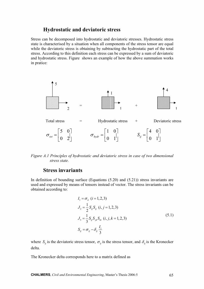
CHALMERS, Civil and Environmental Engineering, Master’s Thesis 2006:5 65
Hydrostatic and deviatoric stress
Stress can be decomposed into hydrostatic and deviatoric stresses. Hydrostatic stress state is characterised by a situation when all components of the stress tensor are equal while the deviatoric stress is obtaining by subtracting the hydrostatic part of the total stress. According to this definition each stress can be expressed by a sum of deviatoric and hydrostatic stress. Figure shows an example of how the above summation works in pratice:
Figure A.1 Principles of hydrostatic and deviatoric stress in case of two dimensional stress state.
Stress invariants
In definition of bounding surface (Equations (5.20) and (5.21)) stress invariants are used and expressed by means of tensors instead of vector. The stress invariants can be obtained according to:
1
2
3
1
( 1, 2,3)1 ( , 1, 2,3)21 ( , , 1, 2,3)3
3
ii
ij ij
ij jk ki
ij ij ij
I i
J S S i j
J S S S i j k
IS
σ
σ δ
= =
= =
= =
= −
(5.1)
where ijS is the deviatoric stress tensor, ijσ is the stress tensor, and ijδ is the Kronecker delta.
The Kronecker delta corresponds here to a matrix defined as
5
2
1
1 1
4
= +
Total stress Hydrostatic stress Deviatoric stress = +
5 0 1 0 4 00 2 0 1 0 1tot hydr ijSσ σ⎡ ⎤ ⎡ ⎤ ⎡ ⎤
= = =⎢ ⎥ ⎢ ⎥ ⎢ ⎥⎣ ⎦ ⎣ ⎦ ⎣ ⎦

CHALMERS, Civil and Environmental Engineering, Master’s Thesis 2006:5 66
1 0 00 1 00 0 1
ijδ⎡ ⎤⎢ ⎥= ⎢ ⎥⎢ ⎥⎣ ⎦
(5.2)
According to the definition of the invariants, the invariants do not change when changing from one orthonormal right-handed basis to another.
An index that occurs exactly twice in a term implies summation. An example can be found in the definition of the first stress invariant:
3
1 11 22 331
ii iii
I σ σ σ σ σ=
= = = + +∑ (5.3)
This implies that dubble summation is needed in order to obtain the second invariant:
3 3
21 1
1 12 2ij ij ij ij
i jJ S S S S
= =
= = ∑∑ (5.4)
In this way it is possible to obtain the values for the searched stress invariants.

CHALMERS, Civil and Environmental Engineering, Master’s Thesis 2006:5 67
APPENDIX B – MATLAB code for modified Maekawa concrete model

CHALMERS, Civil and Environmental Engineering, Master’s Thesis 2006:5 68

CHALMERS, Civil and Environmental Engineering, Master’s Thesis 2006:5 69
%Modified Maekawa Concrete Model.
%according to Diana Model Library
%Version 3.2
%Tests in order to improve model according to the book:
%"Nonlinear mechanics of reinforced concrete" (further called the book)
% of K. Maekawa, A. Pimanmas and H. Okamura.
%%%%%%%%%%%%%%%%%%%%%%%%%%%%%%%%%%%%%%%%%%%%%%%%%%%%%%%%%%%%%%%%%%
%Mikael Szymanski
%Payman Ameen
%%%%%%%%%%%%%%%%%%%%%%%%%%%%%%%%%%%%%%%%%%%%%%%%%%%%%%%%%%%%%%%%%%
%Last modified
%2005.10.25
clear all; close all; clc; format long
%%%%%%%%%%%%%%%%%%%%%%%%%%%%%%%%%%%%%%%%%%%%%%%%%%%%%%%%%%%%%%%%%%
figure(1);
subplot(5,1,1); xlabel('Strain'); ylabel('Time'); hold; grid on;
subplot(5,1,2);xlabel('Strain'); ylabel('Stress');hold; grid on;
subplot(5,1,3);xlabel('Strain'); ylabel('Alpha');hold; grid on;
subplot(5,1,4);xlabel('Strain'); ylabel('ep');hold; grid on;
subplot(5,1,5);xlabel('Strain'); ylabel('K0');hold; grid on;
figure(2);
xlabel('Strain'); ylabel('Stress');hold; grid on;
figure(3);
subplot(2,1,1); xlabel('Strain'); ylabel('Time'); hold; grid on;
subplot(2,1,2);xlabel('Strain'); ylabel('Stress');hold; grid on;
figure(4);
subplot(2,1,1); xlabel('Strain'); ylabel('Stress'); hold; grid on;
subplot(2,1,2);xlabel('Strain'); ylabel('K0');hold; grid on;
%%%%%%%%%%%%%%%%%%%%%%%%%%%%%%%%%%%%%%%%%%%%%%%%%%%%%%%%%%%%%%%%%%
fc=-50; %uniaxial compresive strain.
ec=-0.002; %uniaxial strain at fc.
CHALMERS, Civil and Environmental Engineering, Master’s Thesis 2006:5 70
Ec0=39e3; %2*fc/ec; %initial stiffness acc. to the book.
deps(1)=-10e-6; %total principal strain increment.
iii=1; %counter for unloading in order to estimate.
beta=1; %strain-rate factor acc. to the book.
sigma(iii)=fc; %stress at the beginning of unloading.
sigma0cc=sigma(iii); %current compressive stress acc. to the book.
PN=2; %unloading parameter.
firstloading=1; %if 1 then the loading starts at 1.
nextplasticity=0; %defining if one is continuing plastic deformations
%and thus development of ep. With other words nextplasticity
%defines if we are back on the nevelope curve.
%%%%%%%%%%%%%%%%%%%%%%%%%%%%%%%%%%%%%%%%%%%%%%%%%%%%%%%%%%%%%%%%%%
%strain history (-1)=unloading; (+1)=loading.
%It is possible to modify the lengths of loading and unloading by changing
%the length of aa-counter in reloading and unloading loops, respectively.
for aa=1:200
k(aa)=1;
end
for aa=201:300
k(aa)=-1;
end
for aa=301:350
k(aa)=1;
end
%%%%%%%%%%%%%%%%%%%%%%%%%%%%%%%%%%%%%%%%%%%%%%%%%%%%%%%%%%%%%%%%%%
for i=1:length(k);
epscalc=cumsum(k);
%epsvector(i)=ec+epscalc(i)*deps;
epsvector(i)=epscalc(i)*deps;
end
for i=1:length(k)

CHALMERS, Civil and Environmental Engineering, Master’s Thesis 2006:5 71
eps=epsvector(i);
if (i-1)==0
eps0=ec; %where eps0 is "current stress" according to the book.
else
eps0=epsvector(i-1);
end
if firstloading==1 %| nextplasticity=1;
K0=exp(-0.73*eps/ec*(1-exp(-1.25*eps/ec))); %Fracture parameter.
ep=beta*(eps/ec-20/7*(1-exp(-0.35*eps/ec)))*ec; %plastic strain - not constant!
E0=2; %coefficient acc. to the book
Ec0=E0*fc/ec; %initial stiffness acc. to the book
sigmacc(iii)=K0*Ec0*(eps-ep); %Stress
figure(1); subplot(5,1,1);plot(eps,i);
figure(1); subplot(5,1,2); plot(eps,sigmacc(iii));
%figure(1); subplot(5,1,3); plot(eps,alpha);
figure(1); subplot(5,1,4); plot(eps,ep);
figure(1); subplot(5,1,5); plot(eps,K0);
figure(2); plot(-eps,-sigmacc(iii),'.');
figure(3); subplot(2,1,1); plot(-eps,i,'.');
figure(3); subplot(2,1,2); plot(-eps,-sigmacc(iii),'.');
figure(4); subplot(2,1,1); plot(-eps,-sigmacc(iii));
figure(4); subplot(2,1,2); plot(-eps,K0);
% if (i+1)>length(epsvector)
% disp('end of loading sequence')
if epsvector(i+1)>=eps
firstloading=0; %turning off first loading
sigma0cc=sigmacc(iii); %defines current stress
sigmamax=sigmacc(iii); %defines the maximal value of sigma.

CHALMERS, Civil and Environmental Engineering, Master’s Thesis 2006:5 72
iii=iii+1;
else
iii=iii+1;
end
%disp('first')
elseif eps>ec & eps>eps0 & eps<=0 %compressive unloading.
%break
%K0=exp(-0.73*eps/ec*(1-exp(-1.25*eps/ec))); %Fracture parameter.
%K0=0.95; %0.59471184282946;
%ep=beta*(eps/ec-20/7*(1-exp(-0.35*eps/ec)))*ec; %plastic strain - not constant!
%ep=-2.42e-4; %plastic strain - constant!
alpha=K0^2 + (sigma0cc/(K0*Ec0*(eps0-ep))-K0^2)*((eps-ep)/(eps0-ep))^PN
sigmacc(iii)=K0*Ec0*(eps-ep)*alpha; %Stress.
sigma0cc=sigmacc(iii); %Re-definition of current stress.
% if iii==200
% break
% end
figure(1); subplot(5,1,1);plot(eps,i);
figure(1); subplot(5,1,2); plot(eps,sigmacc(iii));
figure(1); subplot(5,1,3); plot(eps,alpha);
figure(1); subplot(5,1,4); plot(eps,ep);
figure(1); subplot(5,1,5); plot(eps,K0);
figure(2); plot(-eps,-sigmacc(iii),'ro');
figure(3); subplot(2,1,1); plot(-eps,i,'.');
figure(3); subplot(2,1,2); plot(-eps,-sigmacc(iii),'.');
figure(4); subplot(2,1,1); plot(-eps,-sigmacc(iii));
figure(4); subplot(2,1,2); plot(-eps,K0);
iii=iii+1;
sigmacmax=min(sigmacc); %Maximum compressive stress ever experienced in the material.

CHALMERS, Civil and Environmental Engineering, Master’s Thesis 2006:5 73
epsvector2(iii)=eps;
ecmax=min(epsvector2);
%disp('unload')
elseif eps>ec & eps<=eps0 & eps<=0 %compressive reloading.
sigmacc(iii)=sigmacmax-(sigmacmax-sigma0cc)*((ecmax-eps)/(ecmax-eps0));
sigma0cc=sigmacc(iii);
if sigmacc(iii)<=sigmamax
firstloading=1;
else
firstloading=0;
end
figure(1); subplot(5,1,1);plot(eps,i);
figure(1); subplot(5,1,2); plot(eps,sigmacc(iii),'r');
figure(2); plot(-eps,-sigmacc(iii),'o');
figure(3); subplot(2,1,1); plot(-eps,i,'.');
figure(3); subplot(2,1,2); plot(-eps,-sigmacc(iii),'.');
figure(4); subplot(2,1,1); plot(-eps,-sigmacc(iii));
figure(4); subplot(2,1,2); plot(-eps,K0);
iii=iii+1;
%disp('reload');
else
disp('error');
end
if eps>0 & sigmacc(iii)>0
disp('the stress change sign! - tension!')
end
end
figure(6); xlabel('Strain'); ylabel('Stress'); hold; grid on;plot(-epsvector,-sigmacc,'-');

CHALMERS, Civil and Environmental Engineering, Master’s Thesis 2006:5 74

CHALMERS, Civil and Environmental Engineering, Master’s Thesis 2006:5 75
APPENDIX C – MATLAB code for plasticity damage bounding surface model

CHALMERS, Civil and Environmental Engineering, Master’s Thesis 2006:5 76

CHALMERS, Civil and Environmental Engineering, Master’s Thesis 2006:5 77
%Plasticity model for concrete using bounding surface concept.
%Model according to the dissertation of Mr. Taher Abu-Lebdeh
%"Plasticity-damage bounding surface model for concrete under
%cyclic-multiaxial loading", further in comments called "the diss.".
%Version 2.0
%Cyclic-multiaxial loading with damage
%
%%%%%%%%%%%%%%%%%%%%%%%%%%%%%%%%%%%%%%%%%%%%%%%%%%%%%%%%%%%%%%%%%%
%Mikael Szymanski
%Payman Ameen
%%%%%%%%%%%%%%%%%%%%%%%%%%%%%%%%%%%%%%%%%%%%%%%%%%%%%%%%%%%%%%%%%%
%Last modified
%2005.12.10
%%%%%%%%%%%%%%%%%%%%%%%%%%%%%%%%%%%%%%%%%%%%%%%%%%%%%%%%%%%%%%%%%%
clear all; clc; close all;
%%%%%%%%%%%%%%%%%%%%%%%%%%%%%%%%%%%%%%%%%%%%%%%%%%%%%%%%%%%%%%%%%%
%Input parameters
XEO=5656.47%5003.8 % 5656.47%5003.8 %5656.47 %ksi %39e3; %Modulus of elasticity. OBS annan variabel heter E?????????????
XNU=-0.2; %Poisson's ratio.
FC=7.25%5.8%4.918 %7.25; %ksi%compressive strength of plain concrete.
k0=500*FC; %initial value of bulk tangent modulus acc. to the diss.
mstr=0; %assumption about maximum strain ever experienced by the
%material at the beginning of loading (small number, ca. =0).
He=850*FC; %Elastic modulus He.
%%%%%%%%%%%%%%%%%%%%%%%%%%%%%%%%%%%%%%%%%%%%%%%%%%%%%%%%%%%%%%%%%%
%Reading load input.
[SIG1, SIG2, SIG3]=loadingcyclic2%loadingcyclic%loadingmonotonic;%loadingcyclic;
aaa=length(SIG3);

CHALMERS, Civil and Environmental Engineering, Master’s Thesis 2006:5 78
X4=0;
cruo=0;
%c
% i=2;
% sigma1(1)=-10
for I=2:length(SIG3)
%%%%%%%%%%%%%%%%%%%%%%%%%%%%%%%%%%%%%%%%%%%%%%%%%%%%%%%%%%%%%%%%%%
%Estimation of stress invariants and the deviatoric stress components
XI1(I)=SIG1(I)+SIG2(I)+SIG3(I);
XJ2(I)=((SIG1(I)-SIG2(I))^2+(SIG2(I)-SIG3(I))^2+(SIG3(I)-SIG1(I))^2)/6;
S1(I)=(2*SIG1(I)-SIG2(I)-SIG3(I))/3;
S2(I)=(2*SIG2(I)-SIG1(I)-SIG3(I))/3;
S3(I)=(2*SIG3(I)-SIG1(I)-SIG2(I))/3;
XJ3(I)=S1(I)*S2(I)*S3(I);
if XJ2(I)==0
XJ2(I)=SIG3(I)^2/3;
end
%%%%%%%%%%%%%%%%%%%%%%%%%%%%%%%%%%%%%%%%%%%%%%%%%%%%%%%%%%%%%%%%%%
%Determination of the normalized distance d
Z(I)=2.598*XJ3(I)/((XJ2(I))^1.5);
TU(I)=sqrt(2*XJ2(I)/3);
%%%%%%%%%%%%%%%%%%%%%%%%%%%%%%%%%%%%%%%%%%%%%%%%%%%%%%%%%%%%%%%%%%
%CHECKING LOADING CONDITIONS (UNLOADING OR RELAODING)
DELI1(I)=abs(XI1(I))-abs(XI1(I-1));
DELTU(I)=TU(I)-TU(I-1);
if DELI1(I)>=0
XKT(I)=625*FC/(1+0.4*(abs(XI1(I)))^1.35); %bulk tangent modulus for hydrostatic reloading
else
XKT(I)=575*FC; %bulk tangent modulus for hydrostatic unloading
end
if DELTU(I)>=0

CHALMERS, Civil and Environmental Engineering, Master’s Thesis 2006:5 79
X5(I)=DELTU(I-1)*DELTU(I);
if X5(I)>=0
ruc(I)=(-9.237+sqrt(85.328-23.504*(2.53-X4)*(3.1962*XI1(I)/FC-1)))*FC/(5.878*(2.53-X4));
ru(I)=sqrt(2*XJ2(I));
D(I)=(ruc(I)-ru(I))/(ruc(I)-cruo);
else
cruo=sqrt(2*XJ2(I));
ruc(I)=(-9.237+sqrt(85.328-23.504*(2.53-X4)*(3.1962*XI1(I)/FC-1)))*FC/(5.878*(2.53-X4));
ru(I)=sqrt(2*XJ2(I));
D(I)=(ruc(I)-ru(I))/(ruc(I)-cruo);
end
i=-3*FC;
if XI1(I)>=i
hpar(I)=(XI1(I)/FC-0.5)^2/(10*(1.1+Z(I))^0.2);
else
hpar(I)=(-0.82*(XI1(I)/FC+1.45))/(1.1+Z(I))^0.2;
end
y=-150*mstr;
hp(I)=350*FC*(ruc(I)-cruo)*sqrt(D(I))*(10^y)/hpar(I); %plastic modulus for deviaoric reloading
else
X3(I)=DELTU(I-1)*DELTU(I);
if X3(I)>=0
rut(I)=(-16.581+sqrt(274.27-23.504*(2.53-X4)*3.1982*XI1(I)/FC-1))*FC/(5.878*(2.53-X4));
ru(I)=sqrt(2*XJ2(I));
D(I)=(ru(I)+rut(I))/(truo+rut(I));
else
mstr=abs(STR3(I-1));
truo=sqrt(2*XJ2(I));
xmr1=XI1(I-1);
X4=sqrt(-1*log(mstr));

CHALMERS, Civil and Environmental Engineering, Master’s Thesis 2006:5 80
rut(I)=(-16.581+sqrt(274.27-23.504*(2.53-X4)*3.1982*XI1(I)/FC-1))*FC/(5.878*(2.53-X4));
ru(I)=sqrt(2*XJ2(I));
D(I)=(ru(I)+rut(I))/(truo+rut(I));
end
i=-3*FC;
if XI1(I)>=i
hpar(I)=((xmr1/FC-0.5)^2-1.176*(xmr1/FC-0.5)*(XI1(I)/FC-0.5))/(14*(1.1+Z(I))^0.4);
else
hpar(I)=(xmr1/FC-1.45)*((1.16*(XI1(I)/FC-0.5)/(xmr1/FC-0.5))-1)/(1.77*(1.1+Z(I))^0.4);
end
hp(I)=(1.35*D(I)^0.82*FC)/(hpar(I)*(mstr)^0.65*(truo+rut(I))^0.35); %plastic modulus for deviaoric unloading ????truo ruo
end
%%%%%%%%%%%%%%%%%%%%%%%%%%%%%%%%%%%%%%%%%%%%%%%%%%%%%%%%%%%%%%%%%%
%elastic modulus and compaction-dilatancy factor
he=850*FC;
beta(I)=10.25*(mstr^0.23)*(sqrt(D(I))-0.2);
%%%%%%%%%%%%%%%%%%%%%%%%%%%%%%%%%%%%%%%%%%%%%%%%%%%%%%%%%%%%%%%%%%
SIG1I(I)=SIG1(I)-SIG1(I-1);
SIG2I(I)=SIG2(I)-SIG2(I-1);
SIG3I(I)=SIG3(I)-SIG3(I-1);
X1(I)=(S1(I)*SIG1I(I)+S2(I)*SIG2I(I)+S3(I)*SIG3I(I))/(12*hp(I)*TU(I));
X2(I)=(1/(9*XKT(I))-1/(3*he))*(SIG1I(I)+SIG2I(I)+SIG3I(I));
%%%%%%%%%%%%%%%%%%%%%%%%%%%%%%%%%%%%%%%%%%%%%%%%%%%%%%%%%%%%%%%%%%
%determination of the elastic and plastic strain increment
PSTR1I(I)=SIG1I(I)/he+(S1(I)/TU(I)+beta(I)/3)*X1(I)+X2(I);
PSTR2I(I)=SIG2I(I)/he+(S2(I)/TU(I)+beta(I)/3)*X1(I)+X2(I);
PSTR3I(I)=SIG3I(I)/he+(S3(I)/TU(I)+beta(I)/3)*X1(I)+X2(I);
%%%%%%%%%%%%%%%%%%%%%%%%%%%%%%%%%%%%%%%%%%%%%%%%%%%%%%%%%%%%%%%%%%
%THE SECOND PART OF THE MODEL: Strain Increment due to damage

CHALMERS, Civil and Environmental Engineering, Master’s Thesis 2006:5 81
CD(1)=0.05;
TD(1)=0.05;
CD1(1)=0.0289;
CD2(1)=CD1(1);
CD3(1)=CD1(1);
TD1(1)=CD1(1);
TD2(1)=CD1(1);
TD3(1)=CD1(1);
if SIG3I(I)>=0
E(I)=SIG1I(I)/PSTR1I(I);
XNU=-PSTR3I(I)/PSTR1I(I);
else
E(I)=SIG3I(I)/PSTR3I(I);
XNU=-PSTR1I(I)/PSTR3I(I);
end
%%%%%%%%%%%%%%%%%%%%%%%%%%%%%%%%%%%%%%%%%%%%%%%%%%%%%%%%%%%%%%%%%%
%Determination of the hardening parameter ko and the shape factor K
XKO(I)=1+((1.65e-6*(E(I)/FC)^2-2e-3*(E(I)/FC)*(1+XNU))/(1+XNU)^2);
if XKO(I)>=1
CPAR(I)=4.5;
else
CPAR(I)=4.2/(XKO(I)-1);
end
if SIG1(I)<=0
TI1(I)=0;
CI1(I)=(SIG1(I)+SIG2(I)+SIG3(I))/FC;
TJ2(I)=0;
CJ2(I)=((SIG1(I)-SIG2(I))^2+(SIG2(I)-SIG3(I))^2+(SIG3(I)-SIG1(I))^2)/(6*(FC^2));
TS1(I)=0;
TS2(I)=0;

CHALMERS, Civil and Environmental Engineering, Master’s Thesis 2006:5 82
TS3(I)=0;
CS1(I)=(2*SIG1(I)-SIG2(I)-SIG3(I))/3;
CS2(I)=(2*SIG2(I)-SIG1(I)-SIG3(I))/3;
CS3(I)=(2*SIG3(I)-SIG2(I)-SIG1(I))/3;
elseif SIG3(I)>=0
CI1(I)=0;
TI1(I)=(SIG1(I)+SIG2(I)+SIG3(I))/FC;
CJ2(I)=0;
TJ2(I)=((SIG1(I)-SIG2(I))^2+(SIG2(I)-SIG3(I))^2+(SIG3(I)-SIG1(I))^2)/(6*(FC^2));
CS1(I)=0;
CS2(I)=0;
CS3(I)=0;
TS1(I)=(2*SIG1(I)-SIG2(I)-SIG3(I))/3;
TS2(I)=(2*SIG2(I)-SIG1(I)-SIG3(I))/3;
TS3(I)=(2*SIG3(I)-SIG2(I)-SIG1(I))/3;
elseif SIG2(I)>=0
CI1(I)=SIG3(I)/FC;
TI1(I)=(SIG1(I)+SIG2(I))/FC;
CJ2(I)=(SIG3(I)/FC)^2/3;
TJ2(I)=(SIG1(I)^2+SIG2(I)^2+(SIG1(I)-SIG2(I))^2)/(6*(FC^2));
CS1(I)=-SIG3(I)/3;
CS2(I)=CS1(I);
CS3(I)=2*SIG3(I)/3;
TS1(I)=(2*SIG1(I)-SIG2(I))/3;
TS2(I)=(2*SIG2(I)-SIG1(I))/3;
TS3(I)=-(SIG1(I)+SIG2(I))/3;
else
CI1(I)=(SIG2(I)+SIG3(I))/FC;
TI1(I)=SIG1(I)/FC;
CJ2(I)=(SIG2(I)^2+(SIG2(I)-SIG3(I))^2+SIG3(I)^2)/(6*(FC^2));
TJ2(I)=(SIG1(I)^2)/(3*(FC^2));

CHALMERS, Civil and Environmental Engineering, Master’s Thesis 2006:5 83
CS1(I)=-(SIG2(I)+SIG3(I))/3;
CS2(I)=(2*SIG2(I)-SIG3(I))/3;
CS3(I)=(2*SIG3(I)-SIG2(I))/3;
TS1(I)=2*SIG1(I)/3;
TS2(I)=-SIG1(I)/3;
TS3(I)=TS2(I);
end
if CI1(I)<=-1
CK(I)=XKO(I)*(1-((CI1(I)+1)/(CPAR(I)+1))^2);
CALPHA(I)=-XKO(I)/(CPAR(I)+1)^2;
else
CALPHA(I)=(1-XKO(I))/1.716;
CK(I)=1+((1-XKO(I))*(CI1(I)^2+2*CI1(I)-0.716))/1.716;
end
TALPHA(I)=(1-XKO(I))/1.716;
TK(I)=1+((1-XKO(I))*(TI1(I)^2+2*TI1(I)-0.716))/1.716;
GC(I)=25.7/(25+CD(I-1));
GT(I)=10.13/(10+TD(I-1));
%%%%%%%%%%%%%%%%%%%%%%%%%%%%%%%%%%%%%%%%%%%%%%%%%%%%%%%%%%%%%%%%%%
%Damage bounding surface
CRUF(I)=0.3919*FC*(-9.237+sqrt(85.321-10.209*(3.1982*CI1(I)-GC(I))));
TRUF(I)=0.3919*FC*(-16.581+sqrt(274.29-10.209*(3.1962*TI1(I)-GT(I))));
if DELTU(I)>=0
%%%%%%%%%%%%%%%%%%%%%%%%%%%%%%%%%%%%%%%%%%%%%%%%%%%%%%%%%%%%%%%%%%
%the separation distance between a point on the loading surface
%and the corresponding image point on the bounding surface
CDEL(I)=CRUF(I)*abs((1-CK(I)));
TDEL(I)=TRUF(I)*abs((1-TK(I)));
cy=-0.33*sqrt(abs(CD(I-1)));
ty=-0.53*abs(TD(I-1));
%%%%%%%%%%%%%%%%%%%%%%%%%%%%%%%%%%%%%%%%%%%%%%%%%%%%%%%%%%%%%%%%%%
%Estimation of the damage hardenng modulus

CHALMERS, Civil and Environmental Engineering, Master’s Thesis 2006:5 84
HC(I)=(3000*FC*sqrt(CRUF(I)*CDEL(I))*(10^cy))/(CI1(I)-0.5)^2;
HT(I)=(980*FC*sqrt(TRUF(I)*TDEL(I))*(10^ty))/(TI1(I)+0.3)^2;
if CJ2(I)==0
CA(I)=0;
CB(I)=0;
else
CA(I)=((1.2759/(FC^2))+((6.5315/(FC^2))*CK(I))/(2*sqrt(CJ2(I))));
CB(I)=13.038*(CALPHA(I)/FC)*(1+CI1(I))*sqrt(CJ2(I))+12.785*(CALPHA(I)/FC)*CK(I)*CI1(I)*(1+CI1(I))-4*(CALPHA(I)/FC)*CK(I)*(1+CI1(I))*GC(I)+(3.1962/FC)*CK(I)^2;
end
if TJ2(I)==0
TA(I)=0;
TB(I)=0;
else
TA(I)=(1.2759/(FC^2))+((11.7109/(FC^2))*TK(I))/(2*sqrt(TJ2(I))); TB(I)=23.422*(TALPHA(I)/FC)*(1+TI1(I))*sqrt(TJ2(I))+12.785*(TALPHA(I)/FC)*TK(I)*TI1(I)*(1+TI1(I))-4*(TALPHA(I)/FC)*TK(I)*(1+TI1(I))*GT(I)+(3.1982/FC)*TK(I)^2;
end
if CK(I)>=0.4
if CK(I)<1
if TK(I)<1
if SIG3>=0
CD1I(I)=0;
CD2I(I)=0;
CD3I(I)=0;
if SIG1(I)<=0
TD1I(I)=0;
TD2I(I)=0;
TD3I(I)=0;

CHALMERS, Civil and Environmental Engineering, Master’s Thesis 2006:5 85
else
TD1I(I)=2.82e7*(((TA(I)^2*TS1(I)+TA(I)*TB(I))*TS1(I)+(TB(I)^2+TA(I)*TB(I)*TS1(I)))*SIG1I(I)/HT(I));
TD2I(I)=2.82e7*(((TA(I)^2*TS2(I)+TA(I)*TB(I))*TS1(I)+(TB(I)^2+TA(I)*TB(I)*TS2(I)))*SIG1I(I)/HT(I));
TD3I(I)=2.82e7*(((TA(I)^2*TS3(I)+TA(I)*TB(I))*TS1(I)+(TB(I)^2+TA(I)*TB(I)*TS3(I)))*SIG1I(I)/HT(I));
end
if TD1I(I)<0
TD1I(I)=0;
end
if TD2I(I)<0
TD2I(I)=0;
end
if TD3I(I)<0
TD3I(I)=0;
end
else
if HC(I)==0
HC(I)=1e-3;
end
CD1I(I)=520*(((CA(I)^2*CS1(I)+CA(I)*CB(I))*(CS2(I)*SIG2I(I)+CS3(I)*SIG3I(I))+(CB(I)^2+CA(I)*CB(I)*CS1(I))*(SIG2I(I)+SIG3I(I)))/HC(I));
CD2I(I)=520*(((CA(I)^2*CS2(I)+CA(I)*CB(I))*(CS2(I)*SIG2I(I)+CS3(I)*SIG3I(I))+(CB(I)^2+CA(I)*CB(I)*CS2(I))*(SIG2I(I)+SIG3I(I)))/HC(I));
CD3I(I)=520*(((CA(I)^2*CS3(I)+CA(I)*CB(I))*(CS2(I)*SIG2I(I)+CS3(I)*SIG3I(I))+(CB(I)^2+CA(I)*CB(I)*CS3(I))*(SIG2I(I)+SIG3I(I)))/HC(I));
if CD1I(I)<0
CD1I(I)=0;
end
if CD2I(I)<0

CHALMERS, Civil and Environmental Engineering, Master’s Thesis 2006:5 86
CD2I(I)=0;
end
if CD3I(I)<0
CD3I(I)=0;
end
if SIG1(I)<=0
TD1I(I)=0;
TD2I(I)=0;
TD3I(I)=0;
else
TD1I(I)=2.82e7*(((TA(I)^2*TS1(I)+TA(I)*TB(I))*TS1(I)+(TB(I)^2+TA(I)*TB(I)*TS1(I)))*SIG1I(I)/HT(I));
TD2I(I)=2.82e7*(((TA(I)^2*TS2(I)+TA(I)*TB(I))*TS1(I)+(TB(I)^2+TA(I)*TB(I)*TS2(I)))*SIG1I(I)/HT(I));
TD3I(I)=2.82e7*(((TA(I)^2*TS3(I)+TA(I)*TB(I))*TS1(I)+(TB(I)^2+TA(I)*TB(I)*TS3(I)))*SIG1I(I)/HT(I));
end
if TD1I(I)<0
TD1I(I)=0;
end
if TD2I(I)<0
TD2I(I)=0;
end
if TD3I(I)<0
TD3I(I)=0;
end
end
else
HT(I)=(-10.13/(TD(I-1)*(10+TD(I-1))^2))*(TD1(I-1)*(TA(I)*TS1(I)+TB(I))+TD2(I-1)*(TA(I)*TS2(I)+TB(I))+TD3(I-1)*(TA(I)*TS3(I)+TB(I)));
if SIG3>=0

CHALMERS, Civil and Environmental Engineering, Master’s Thesis 2006:5 87
CD1I(I)=0;
CD2I(I)=0;
CD3I(I)=0;
if SIG1(I)<=0
TD1I(I)=0;
TD2I(I)=0;
TD3I(I)=0;
else
TD1I(I)=2.82e7*(((TA(I)^2*TS1(I)+TA(I)*TB(I))*TS1(I)+(TB(I)^2+TA(I)*TB(I)*TS1(I)))*SIG1I(I)/HT(I));
TD2I(I)=2.82e7*(((TA(I)^2*TS2(I)+TA(I)*TB(I))*TS1(I)+(TB(I)^2+TA(I)*TB(I)*TS2(I)))*SIG1I(I)/HT(I));
TD3I(I)=2.82e7*(((TA(I)^2*TS3(I)+TA(I)*TB(I))*TS1(I)+(TB(I)^2+TA(I)*TB(I)*TS3(I)))*SIG1I(I)/HT(I));
end
if TD1I(I)<0
TD1I(I)=0;
end
if TD2I(I)<0
TD2I(I)=0;
end
if TD3I(I)<0
TD3I(I)=0;
end
else
if HC(I)==0
HC(I)=1e-3;
end CD1I(I)=520*(((CA(I)^2*CS1(I)+CA(I)*CB(I))*(CS2(I)*SIG2I(I)+CS3(I)*SIG3I(I))+(CB(I)^2+CA(I)*CB(I)*CS1(I))*(SIG2I(I)+SIG3I(I)))/HC(I));
CD2I(I)=520*(((CA(I)^2*CS2(I)+CA(I)*CB(I))*(CS2(I)*SIG2I(I)+CS3(I)*SIG3I(I))+(CB(I)^2+CA(I)*CB(I)*CS2(I))*(SIG2I(I)+SIG3I(I)))/HC(I));

CHALMERS, Civil and Environmental Engineering, Master’s Thesis 2006:5 88
CD3I(I)=520*(((CA(I)^2*CS3(I)+CA(I)*CB(I))*(CS2(I)*SIG2I(I)+CS3(I)*SIG3I(I))+(CB(I)^2+CA(I)*CB(I)*CS3(I))*(SIG2I(I)+SIG3I(I)))/HC(I));
if CD1I(I)<0
CD1I(I)=0;
end
if CD2I(I)<0
CD2I(I)=0;
end
if CD3I(I)<0
CD3I(I)=0;
end
if SIG1(I)<=0
TD1I(I)=0;
TD2I(I)=0;
TD3I(I)=0;
else
TD1I(I)=2.82e7*(((TA(I)^2*TS1(I)+TA(I)*TB(I))*TS1(I)+(TB(I)^2+TA(I)*TB(I)*TS1(I)))*SIG1I(I)/HT(I));
TD2I(I)=2.82e7*(((TA(I)^2*TS2(I)+TA(I)*TB(I))*TS1(I)+(TB(I)^2+TA(I)*TB(I)*TS2(I)))*SIG1I(I)/HT(I));
TD3I(I)=2.82e7*(((TA(I)^2*TS3(I)+TA(I)*TB(I))*TS1(I)+(TB(I)^2+TA(I)*TB(I)*TS3(I)))*SIG1I(I)/HT(I));
end
if TD1I(I)<0
TD1I(I)=0;
end
if TD2I(I)<0
TD2I(I)=0;
end
if TD3I(I)<0
TD3I(I)=0;
end

CHALMERS, Civil and Environmental Engineering, Master’s Thesis 2006:5 89
end
end
else
HC(I)=(-25.7/(CD(I-1)*(25+CD(I-1))^2))*(CD1(I-1)*(CA(I)*CS1(I)+CB(I))+CD2(I-1)*(CA(I)*CS2(I)+CB(I))+CD3(I-1)*(CA(I)*CS3(I)+CB(I)));
if TK(I)<1
if SIG3>=0
CD1I(I)=0;
CD2I(I)=0;
CD3I(I)=0;
if SIG1(I)<=0
TD1I(I)=0;
TD2I(I)=0;
TD3I(I)=0;
else
TD1I(I)=2.82e7*(((TA(I)^2*TS1(I)+TA(I)*TB(I))*TS1(I)+(TB(I)^2+TA(I)*TB(I)*TS1(I)))*SIG1I(I)/HT(I));
TD2I(I)=2.82e7*(((TA(I)^2*TS2(I)+TA(I)*TB(I))*TS1(I)+(TB(I)^2+TA(I)*TB(I)*TS2(I)))*SIG1I(I)/HT(I));
TD3I(I)=2.82e7*(((TA(I)^2*TS3(I)+TA(I)*TB(I))*TS1(I)+(TB(I)^2+TA(I)*TB(I)*TS3(I)))*SIG1I(I)/HT(I));
end
if TD1I(I)<0
TD1I(I)=0;
end
if TD2I(I)<0
TD2I(I)=0;
end
if TD3I(I)<0
TD3I(I)=0;
end
else
CHALMERS, Civil and Environmental Engineering, Master’s Thesis 2006:5 90
if HC(I)==0
HC(I)=1e-3;
end
CD1I(I)=520*(((CA(I)^2*CS1(I)+CA(I)*CB(I))*(CS2(I)*SIG2I(I)+CS3(I)*SIG3I(I))+(CB(I)^2+CA(I)*CB(I)*CS1(I))*(SIG2I(I)+SIG3I(I)))/HC(I));
CD2I(I)=520*(((CA(I)^2*CS2(I)+CA(I)*CB(I))*(CS2(I)*SIG2I(I)+CS3(I)*SIG3I(I))+(CB(I)^2+CA(I)*CB(I)*CS2(I))*(SIG2I(I)+SIG3I(I)))/HC(I));
CD3I(I)=520*(((CA(I)^2*CS3(I)+CA(I)*CB(I))*(CS2(I)*SIG2I(I)+CS3(I)*SIG3I(I))+(CB(I)^2+CA(I)*CB(I)*CS3(I))*(SIG2I(I)+SIG3I(I)))/HC(I));
if CD1I(I)<0
CD1I(I)=0;
end
if CD2I(I)<0
CD2I(I)=0;
end
if CD3I(I)<0
CD3I(I)=0;
end
if SIG1(I)<=0
TD1I(I)=0;
TD2I(I)=0;
TD3I(I)=0;
else
TD1I(I)=2.82e7*(((TA(I)^2*TS1(I)+TA(I)*TB(I))*TS1(I)+(TB(I)^2+TA(I)*TB(I)*TS1(I)))*SIG1I(I)/HT(I));
TD2I(I)=2.82e7*(((TA(I)^2*TS2(I)+TA(I)*TB(I))*TS1(I)+(TB(I)^2+TA(I)*TB(I)*TS2(I)))*SIG1I(I)/HT(I));
TD3I(I)=2.82e7*(((TA(I)^2*TS3(I)+TA(I)*TB(I))*TS1(I)+(TB(I)^2+TA(I)*TB(I)*TS3(I)))*SIG1I(I)/HT(I));
end

CHALMERS, Civil and Environmental Engineering, Master’s Thesis 2006:5 91
if TD1I(I)<0
TD1I(I)=0;
end
if TD2I(I)<0
TD2I(I)=0;
end
if TD3I(I)<0
TD3I(I)=0;
end
end
else
HT(I)=(-10.13/(TD(I-1)*(10+TD(I-1))^2))*(TD1(I-1)*(TA(I)*TS1(I)+TB(I))+TD2(I-1)*(TA(I)*TS2(I)+TB(I))+TD3(I-1)*(TA(I)*TS3(I)+TB(I)));
if SIG3>=0
CD1I(I)=0;
CD2I(I)=0;
CD3I(I)=0;
if SIG1(I)<=0
TD1I(I)=0;
TD2I(I)=0;
TD3I(I)=0;
else
TD1I(I)=2.82e7*(((TA(I)^2*TS1(I)+TA(I)*TB(I))*TS1(I)+(TB(I)^2+TA(I)*TB(I)*TS1(I)))*SIG1I(I)/HT(I));
TD2I(I)=2.82e7*(((TA(I)^2*TS2(I)+TA(I)*TB(I))*TS1(I)+(TB(I)^2+TA(I)*TB(I)*TS2(I)))*SIG1I(I)/HT(I));
TD3I(I)=2.82e7*(((TA(I)^2*TS3(I)+TA(I)*TB(I))*TS1(I)+(TB(I)^2+TA(I)*TB(I)*TS3(I)))*SIG1I(I)/HT(I));
end
if TD1I(I)<0
CHALMERS, Civil and Environmental Engineering, Master’s Thesis 2006:5 92
TD1I(I)=0;
end
if TD2I(I)<0
TD2I(I)=0;
end
if TD3I(I)<0
TD3I(I)=0;
end
else
if HC(I)==0
HC(I)=1e-3;
end
CD1I(I)=520*(((CA(I)^2*CS1(I)+CA(I)*CB(I))*(CS2(I)*SIG2I(I)+CS3(I)*SIG3I(I))+(CB(I)^2+CA(I)*CB(I)*CS1(I))*(SIG2I(I)+SIG3I(I)))/HC(I));
CD2I(I)=520*(((CA(I)^2*CS2(I)+CA(I)*CB(I))*(CS2(I)*SIG2I(I)+CS3(I)*SIG3I(I))+(CB(I)^2+CA(I)*CB(I)*CS2(I))*(SIG2I(I)+SIG3I(I)))/HC(I));
CD3I(I)=520*(((CA(I)^2*CS3(I)+CA(I)*CB(I))*(CS2(I)*SIG2I(I)+CS3(I)*SIG3I(I))+(CB(I)^2+CA(I)*CB(I)*CS3(I))*(SIG2I(I)+SIG3I(I)))/HC(I));
if CD1I(I)<0
CD1I(I)=0;
end
if CD2I(I)<0
CD2I(I)=0;
end
if CD3I(I)<0
CD3I(I)=0;
end

CHALMERS, Civil and Environmental Engineering, Master’s Thesis 2006:5 93
if SIG1(I)<=0
TD1I(I)=0;
TD2I(I)=0;
TD3I(I)=0;
else
TD1I(I)=2.82e7*(((TA(I)^2*TS1(I)+TA(I)*TB(I))*TS1(I)+(TB(I)^2+TA(I)*TB(I)*TS1(I)))*SIG1I(I)/HT(I));
TD2I(I)=2.82e7*(((TA(I)^2*TS2(I)+TA(I)*TB(I))*TS1(I)+(TB(I)^2+TA(I)*TB(I)*TS2(I)))*SIG1I(I)/HT(I));
TD3I(I)=2.82e7*(((TA(I)^2*TS3(I)+TA(I)*TB(I))*TS1(I)+(TB(I)^2+TA(I)*TB(I)*TS3(I)))*SIG1I(I)/HT(I));
end
if TD1I(I)<0
TD1I(I)=0;
end
if TD2I(I)<0
TD2I(I)=0;
end
if TD3I(I)<0
TD3I(I)=0;
end
end
end
end
else
CD1I(I)=0;
CD2I(I)=0;
CD3I(I)=0;
TD1I(I)=0;
TD2I(I)=0;
TD3I(I)=0;
end
CHALMERS, Civil and Environmental Engineering, Master’s Thesis 2006:5 94
else
CD1(I)=0;
CD2(I)=0;
CD3(I)=0;
TD1(I)=0;
TD2(I)=0;
TD3(I)=0;
CD1I(I)=0;
CD2I(I)=0;
CD3I(I)=0;
TD1I(I)=0;
TD2I(I)=0;
TD3I(I)=0;
end
CD1(I)=CD1I(I)+CD1(I-1);
CD2(I)=CD2I(I)+CD2(I-1);
CD3(I)=CD3I(I)+CD3(I-1);
TD1(I)=TD1I(I)+TD1(I-1);
TD2(I)=TD2I(I)+TD2(I-1);
TD3(I)=TD3I(I)+TD3(I-1);
if CD1(I)>=0.7
CD1(I)=0.7
end
if CD2(I)>=0.7
CD2(I)=0.7
end
if CD3(I)>=0.7
CD3(I)=0.7
end
%%%%%%%%%%%%%%%%%%%%%%%%%%%%%%%%%%%%%%%%%%%%%%%%%%%%%%%%%%%%%%%%%%
%Damage parameters
CHALMERS, Civil and Environmental Engineering, Master’s Thesis 2006:5 95
CD(I)=sqrt(CD1(I)^2+CD2(I)^2+CD3(I)^2);
TD(I)=sqrt(TD1(I)^2+TD2(I)^2+TD3(I)^2);
%%%%%%%%%%%%%%%%%%%%%%%%%%%%%%%%%%%%%%%%%%%%%%%%%%%%%%%%%%%%%%%%%%
%Components of the compliance tensor for tensile stresses
C11(I)=1/(XEO*(1-4*TD1(I)));
C12(I)=-XNU/XEO;
C13(I)=C12(I);
C14(I)=C12(I);
C15(I)=1/(XEO*(1-4*TD2(I)));
C16(I)=C12(I);
C17(I)=C13(I);
C18(I)=C16(I);
C19(I)=1/(XEO*(1-4*TD3(I)));
%%%%%%%%%%%%%%%%%%%%%%%%%%%%%%%%%%%%%%%%%%%%%%%%%%%%%%%%%%%%%%%%%%
%Components of the compliance tensor for compressive stresses
C21(I)=1/(XEO*(1-0.1*CD2(I))*(1-0.1*CD3(I)));
C22(I)=-XNU/(XEO*(1-CD1(I))*(1-CD2(I)));
C23(I)=-XNU/(XEO*(1-CD1(I))*(1-CD3(I)));
C24(I)=C22(I);
C25(I)=1/(XEO*(1-0.1*CD1(I))*(1-0.1*CD3(I)));
C26(I)=-XNU/(XEO*(1-CD2(I))*(1-CD3(I)));
C27(I)=C23(I);
C28(I)=C26(I);
C29(I)=1/(XEO*(1-0.1*CD1(I))*(1-0.1*CD2(I)));
%%%%%%%%%%%%%%%%%%%%%%%%%%%%%%%%%%%%%%%%%%%%%%%%%%%%%%%%%%%%%%%%%%
%components of the rate compliance tensor for tensile stresses
DC11(I)=4*TD1I(I)/(XEO*(1-4*TD1(I))^2);
DC12(I)=4*TD2I(I)/(XEO*(1-4*TD2(I))^2);
DC13(I)=4*TD3I(I)/(XEO*(1-4*TD3(I))^2);
%%%%%%%%%%%%%%%%%%%%%%%%%%%%%%%%%%%%%%%%%%%%%%%%%%%%%%%%%%%%%%%%%%
%components of the rate compliance tensor for compressive stresses
CHALMERS, Civil and Environmental Engineering, Master’s Thesis 2006:5 96
DC21(I)=0.1*((1-0.1*CD3(I))*CD2I(I)+(1-0.1*CD2(I))*CD3I(I))/(XEO*(1-0.1*CD2(I))^2*(1-0.1*CD3(I))^2);
DC22(I)=-XNU*((1-CD2(I))*CD1I(I)+(1-CD1(I))*CD2I(I))/(XEO*(1-CD1(I))^2*(1-CD2(I))^2);
DC23(I)=-XNU*((1-CD3(I))*CD1I(I)+(1-CD1(I))*CD3I(I))/(XEO*(1-CD1(I))^2*(1-CD3(I))^2);
DC24(I)=DC22(I);
DC25(I)=0.1*((1-0.1*CD3(I))*CD1I(I)+(1-0.1*CD1(I))*CD3I(I))/(XEO*(1-0.1*CD1(I))^2*(1-0.1*CD3(I))^2);
DC26(I)=-XNU*((1-CD3(I))*CD2I(I)+(1-CD2(I))*CD3I(I))/(XEO*(1-CD2(I))^2*(1-CD3(I))^2);
DC27(I)=DC23(I);
DC28(I)=DC26(I);
DC29(I)=0.1*((1-0.1*CD2(I))*CD1I(I)+(1-0.1*CD1(I))*CD2I(I))/(XEO*(1-0.1*CD1(I))^2*(1-0.1*CD2(I))^2);
%%%%%%%%%%%%%%%%%%%%%%%%%%%%%%%%%%%%%%%%%%%%%%%%%%%%%%%%%%%%%%%%%%
%Strain increment due to damage
if SIG1(I)<0
DSTR1I(I)=C21(I)*SIG1I(I)+DC21(I)*SIG1(I)+C22(I)*SIG2I(I)+C23(I)*SIG3I(I)+DC22(I)*SIG2(I)+DC23(I)*SIG3(I);
DSTR2I(I)=C24(I)*SIG1I(I)+C25(I)*SIG2I(I)+C26(I)*SIG3I(I)+DC24(I)*SIG1(I)+DC25(I)*SIG2(I)+DC26(I)*SIG3(I); %?C28? kanske C26
DSTR3I(I)=C27(I)*SIG1I(I)+C28(I)*SIG2I(I)+C29(I)*SIG3I(I)+DC27(I)*SIG1(I)+DC28(I)*SIG2(I)+DC29(I)*SIG3(I);
elseif SIG3(I)>=0
DSTR1I(I)=C11(I)*SIG1I(I)+DC11(I)*SIG1(I)+C12(I)*SIG2I(I)+C13(I)*SIG3I(I);
DSTR2I(I)=C14(I)*SIG1I(I)+C15(I)*SIG2I(I)+C16(I)*SIG3I(I)+DC12(I)*SIG2(I);
DSTR3I(I)=C17(I)*SIG1I(I)+C18(I)*SIG2I(I)+C19(I)*SIG3I(I)+DC13(I)*SIG3(I);
elseif SIG2(I)>=0 DSTR1I(I)=C11(I)*SIG1I(I)+DC11(I)*SIG1(I)+C12(I)*SIG2I(I)+C23(I)*SIG3I(I)+DC23(I)*SIG3(I); DSTR2I(I)=C14(I)*SIG1I(I)+C15(I)*SIG2I(I)+C26(I)*SIG3I(I)+DC12(I)*SIG2(I)+DC26(I)*SIG3(I); DSTR3I(I)=C17(I)*SIG1I(I)+C18(I)*SIG2I(I)+C29(I)*SIG3I(I)+DC29(I)*SIG3(I);
else
DSTR1I(I)=C11(I)*SIG1I(I)+DC11(I)*SIG1(I)+C22(I)*SIG2I(I)+C23(I)*SIG3I(I)+DC

CHALMERS, Civil and Environmental Engineering, Master’s Thesis 2006:5 97
22(I)*SIG2(I)+DC23(I)*SIG3(I); DSTR2I(I)=C14(I)*SIG1I(I)+C25(I)*SIG2I(I)+C26(I)*SIG3I(I)+DC25(I)*SIG2(I)+DC26(I)*SIG3(I); DSTR3I(I)=C17(I)*SIG1I(I)+C28(I)*SIG2I(I)+C29(I)*SIG3I(I)+DC28(I)*SIG2(I)+DC29(I)*SIG3(I);
end
STR1(1)=0.0;
STR2(1)=0.0;
STR3(1)=0.0;
%%%%%%%%%%%%%%%%%%%%%%%%%%%%%%%%%%%%%%%%%%%%%%%%%%%%%%%%%%%%%%%%%%
%Calculating the total strain
STR1(I)=PSTR1I(I)+DSTR1I(I)+STR1(I-1);
STR2(I)=PSTR2I(I)+DSTR2I(I)+STR2(I-1);
STR3(I)=PSTR3I(I)+DSTR3I(I)+STR3(I-1);
I
% figure(2); hold on;
% plot(SIG3, mstr)
str3(I)=sum(PSTR3I);
str2(I)=sum(PSTR2I);
str1(I)=sum(PSTR1I);
end
figure(1); hold on; grid on;
plot(STR3, SIG3);
%plot(str3, SIG3,'r');
%plot(str2, SIG3);