fault diagnosis methods for district heating substations 5 fault detection method of a heat...

1

VTT TIEDOTTEITA - MEDDELANDEN - RESEARCH NOTES 1780

Fault diagnosis methodsfor district heating substations

Jouko Pakanen, Juhani Hyvärinen, Juha Kuismin &

Markku Ahonen

VTT Building Technology

ISBN 951-38-4975-9ISSN 1235-0605Copyright © Valtion teknillinen tutkimuskeskus (VTT) 1996

JULKAISIJA – UTGIVARE – PUBLISHER

Valtion teknillinen tutkimuskeskus (VTT), Vuorimiehentie 5, PL 2000, 02044 VTTpuh. vaihde (09) 4561, faksi (09) 456 4374

Statens tekniska forskningscentral (VTT), Bergsmansvägen 5, PB 2000, 02044 VTTtel. växel (09) 4561, fax (09) 456 4374

Technical Research Centre of Finland (VTT), Vuorimiehentie 5, P.O.Box 2000, FIN–02044 VTT, Finlandphone internat. + 358 9 4561, fax + 358 9 456 4374

VTT Rakennustekniikka, Rakennusfysiikka, talo- ja palotekniikka, Kaitoväylä 1, PL 18021, 90571 OULUpuh. vaihde (08) 551 2111, faksi (08) 551 2090

VTT Byggnadsteknik, Byggnadsfysik, hus- och brandteknik, Kaitoväylä 1, PB 18021, 90571 OULUtel. växel (08) 551 2111, fax (08) 551 2090

VTT Building Technology, Building Physics, Building Services and Fire Technology,Kaitoväylä 1, P.O.Box 18021, FIN-90571 OULU, Finlandphone internat. + 358 8 551 2111, fax + 358 8 551 2090

Technical editing Leena Ukskoski

VTT OFFSETPAINO, ESPOO 1996

3

Pakanen, Jouko, Hyvärinen, Juhani, Kuismin, Juha & Ahonen, Markku. Fault diagnosis methods fordistrict heating substations. Espoo 1996, Technical Research Centre of Finland, VTT Tiedotteita -Meddelanden - Research Notes 1780. 70 p.

UDC 697.1:697.34:681.518.5Keywords heating, district heating, substations, fault analysis, automation, control systems,

nstruments, methods, valves, heat exchangers

ABSTRACT

A district heating substation is a demanding process for fault diagnosis. The processis nonlinear, load conditions of the district heating network change unpredictablyand standard instrumentation is designed only for control and local monitoringpurposes, not for automated diagnosis. Extra instrumentation means additional cost,which is usually not acceptable to consumers.

That is why all conventional methods are not applicable in this environment. Thepaper presents five different approaches to fault diagnosis. While developing themethods, various kinds of pragmatic aspects and robustness had to be considered inorder to achieve practical solutions. The presented methods are: classification offaults using performance indexing, static and physical modelling of processequipment, energy balance of the process, interactive fault tree reasoning andstatistical tests. The methods are applied to a control valve, a heat exchanger, a mudseparating device and the whole process. The developed methods are verified inpractice using simulation, emulation or field tests.

4

PREFACE

This paper is a collection of fault diagnosis methods to be applied in district heatingsubstations. The objective of the research was to develop practical fault diagnosis incooperation with HVAC companies. The work is part of the Finnish contribution inIEA Annex 25, which concerns real-time simulation of HVAC systems for buildingoptimization, fault detection and diagnosis. The research was financed byTechnology Development Centre of Finland (TEKES), Technical Research Centreof Finland (VTT) and the following companies: Halton Oy, Oilon Oy and StenforsKy.

The paper presents five different approaches to fault detection and isolation. Themethods were developed and written during the years 1992 - 1994 and most of themhave not been published before. Some changes were made afterwards in order toupdate the contents. The method presented in chapter 4 is written by JuhaniHyvärinen and that in chapter 5 by Markku Ahonen & Juha Kuismin. Chapters 3, 6and 7 present methods written by Jouko Pakanen.

5

TABLE OF CONTENTS

ABSTRACT 3

PREFACE 4

TABLE OF CONTENTS 5

NOMENCLATURE 7

1 INTRODUCTION 9 1.1 Benefits of fault diagnosis 9 1.2 Applied principles 9 1.3 Selected approach 10

2 DISTRICT HEATING SUBSTATION 11 2.1 System description 11 2.2 Domestic hot water 12 2.3 Heating network 12 2.4 Typical faults in a substation 12 2.5 Problems in fault diagnosis of a substation 13

3 CLASSIFICATION OF FAULTS AS A METHOD TO ELIMINATE PROBLEMS OF THRESHOLD ADJUSTMENT 15 3.1 Introduction 15 3.2 Problems of threshold adjustment 15 3.3 Increasing the robustness of fault detection 16 3.4 Performance index 16 3.5 Features 17 3.6 Practical fault grades 18 3.7 Application of the performance classifier 18 3.8 An example: Fault detection of sensory instruments 20 3.9 Summary 23

4 FAULT DETECTION METHOD FOR SUBSTATION PRIMARY FLOW ROUTE AND CONTROL VALVE 25 4.1 Introduction 25 4.2 Outline of the process and the method 26 4.3 Fault detection method 27 4.4 Results 33 4.5 Conclusions 36

6

5 FAULT DETECTION METHOD OF A HEAT EXCHANGER 37 5.1 Introduction 37 5.2 Description of the method 37 5.3 Threshold calculation 40 5.4 Tuning of the method 40 5.5 Upper level reasoning 41 5.6 Result examples 43 5.7 Conclusions 47

6 INTERACTIVE FAULT TREE REASONING 50 6.1 Introduction 50 6.2 Faults localized by an expert user 50 6.3 Faults localized by an expert controller 50 6.4 An intermediate form of the two methods 51 6.5 Instrumentation requirements 51 6.6 Diagnostic tests 52 6.7 More specific fault detection 52 6.8 Selection of the fault tree procedure 52 6.9 Dealing with uncertain information 53 6.10 Applicability 53 6.11 The method applied in a district heating substation 53 6.12 Conclusions 55

7 DETECTING BLOCKAGE OF A MUD SEPARATING 58 DEVICE USING A STATISTICAL TEST 7.1 Introduction 58 7.2 The mud separating device and symptoms of blocking 58 7.3 Monitoring operation and symptoms of the mud filter 59 7.4 Statistical testing

59 7.5 Measurements 62 7.6 Alarm limits 64 7.7 Tuning and start up of the method 64 7.8 Fault selectivity 64 7.9 Test results 65 7.10 Conclusions 67

REFERENCES 68

7

NOMENCLATURE

E(x) Expected value of xD2(x) Variance of xF Feature vectorH0 Null hypothesisH1 Alternate hypothesisJ Performance indexK process amplificationP ProbabilityQ heat power [kW]S Finite setT temperature [°C]∆T Temperature difference [°C]Ua Absolute limitUd Dynamical limitUs Saturation limitX Estimator of a meanZs Constant flow resistance of a heat exchanger and pipeline

a Parameterb Parameterc Coefficient, number of fault gradescp Specific heat capacity [kJ/kg°C]dp Pressure differencedt Time differential [s]e Residualf Coefficientg Coefficientk Sample time [s], step size of a predictorkr Reliability coefficientkvc Manufacturer specific parameter for a valve kv-valuen Sample sizene Manufacturer specific parameter for a control valve characteristicsnp Manufacturer specific parameter for a control valve characteristicsp Parameterqm Mass flow [kg/s]qv Volume flow [dm3/s]r Residuals Laplace operatort Time variable, test parametertau Time constant [s]th Thresholdu Input of a process, control signal

8

~ Predicted value of uy Output of a processz Test parameterx Variable, random variable, feature componentx Feature vector

Ω Set of fault gradesη heat transfer efficiencyλ Deviationµ Meanσ Standard deviationσ2 Varianceω Fault grade

subscripts1 primary side of heat exchanger2 secondary side of heat exchanger

9

1 INTRODUCTION

1.1 BENEFITS OF FAULT DIAGNOSIS

Fault detection and isolation (FDI) methods applied in buildings result in severalbenefits. One benefit is reduced energy consumption. Excessive energy consumptionof buildings caused by fouling dampers, sticking valves, drifting controls and otherfaults may be considerable if the faults are not detected and repaired in time. Besidesenergy savings other benefits are also obvious. These include: water savings,reduced maintenance costs, lower safety and health risks and increased quality ofliving.

Generally, a real-time fault detection system can be used to monitor the process in abuilding and to detect, isolate and even predict faults that may exist or develop inthem. In an ideal case, the system should isolate the original fault and issueinstructions on how to eliminate it. A natural solution would be to provide abuilding automation system or an energy management system (BEM) with on-linediagnostic methods and procedures. However, this kind of FDI system has been onlypartly attained in practice. This is also true for the benefits mentioned above.

1.2 APPLIED PRINCIPLES

Although some diagnostic methods and procedures are already included inautomated processes, their extensive and effective utilization has not yet begun. Thisis also true for processes in buildings. One reason is the lack of robustness of FDImethods. Due to modelling uncertainties and disturbances, the robustness problem isalways present in diagnostic systems. Something can be done to alleviate theproblems by careful design of the FDI method. Such solutions and suggestions formodel-based methods are presented by Gertler (1988), Frank (1994) and Patton(1994). However, the robustness problem concerns not only the diagnostic methodbut the whole diagnostic system. Concentrating only on diagnostic methods does notsolve the problem. Robustness can be partly improved by choosing correctalternatives during system design. These include, for instance, the diagnosticmethod, the level of automation and instrumentation, the role of the user, etc. Thefinal solution is a compromise which also positively influences robustness. Therobustness problem is difficult to solve, but when practical diagnostic methods aretargeted, robust solutions must be the first choice.

Besides robustness, pragmatic aspects (Kurki 1995, Steels 1990, Leitch & Gallanti1992) of the HVAC process and its environment also need to be considered whenthe objective is practical implementation of FDI. These basic issues are seldompresented in FDI publications, although they definitely have an influence on FDImethod development.

10

A brief definition of a practical FDI system is difficult, but some general, qualitativeproperties can be stated. A practical FDI system has more or less the followingproperties. Such a system

- Needs only a few input data submitted by the user.- Needs only domain knowledge for initiation or updating.- Adapts easily to new faults.- Does not disturb normal operation of the process.- Needs no human assistance during detection or isolation.- Causes no additional energy/fuel consumption.- Requires only a short training period/a few training data.- Applies to many kinds of HVAC processes; generic over processes.- Applies to many kinds of faults; generic over faults.- Supports both fault detection and isolation.- Needs only an uncomplicated process model.- Is easy to configure to new applications.- Is easy to embed and integrate in a BEM.- Requires only a minimum or moderate amount of work/costs for development and implementation.- Requires no additional instrumentation.

The list is not exhaustive and some aspects may be changed or omitted, dependingon the application. However, it is obvious that these requirements can be only partlyfulfilled. Some methods follow the design guidelines more carefully than others, butthe final solution is still a compromise for all diagnostic approaches. Although therequirements are demanding, it is reasonable to analyze and compare diagnosticmethods and systems using the above aspects before proceeding to design andimplementation.

1.3 SELECTED APPROACH

This paper presents several FDI methods to be applied in a district heatingsubstation. A starting point for their design is to achieve robustness and to follow theguidelines set by the pragmatic aspects.

Most of the methods are proven by simulating, emulating or field testing. But noneof them has been implemented in an automation system or a BEM. So, the followingdescription clarifies concepts, restrictions and requirements of the methods morethan their detailed implementation procedures. Although many of the methods arenot yet directly applicable in practice, the diversity of approaches illustrates differentsolutions and reveals diagnostic problems in the district heating environment.

11

2 DISTRICT HEATING SUBSTATION

2.1 SYSTEM DESCRIPTION

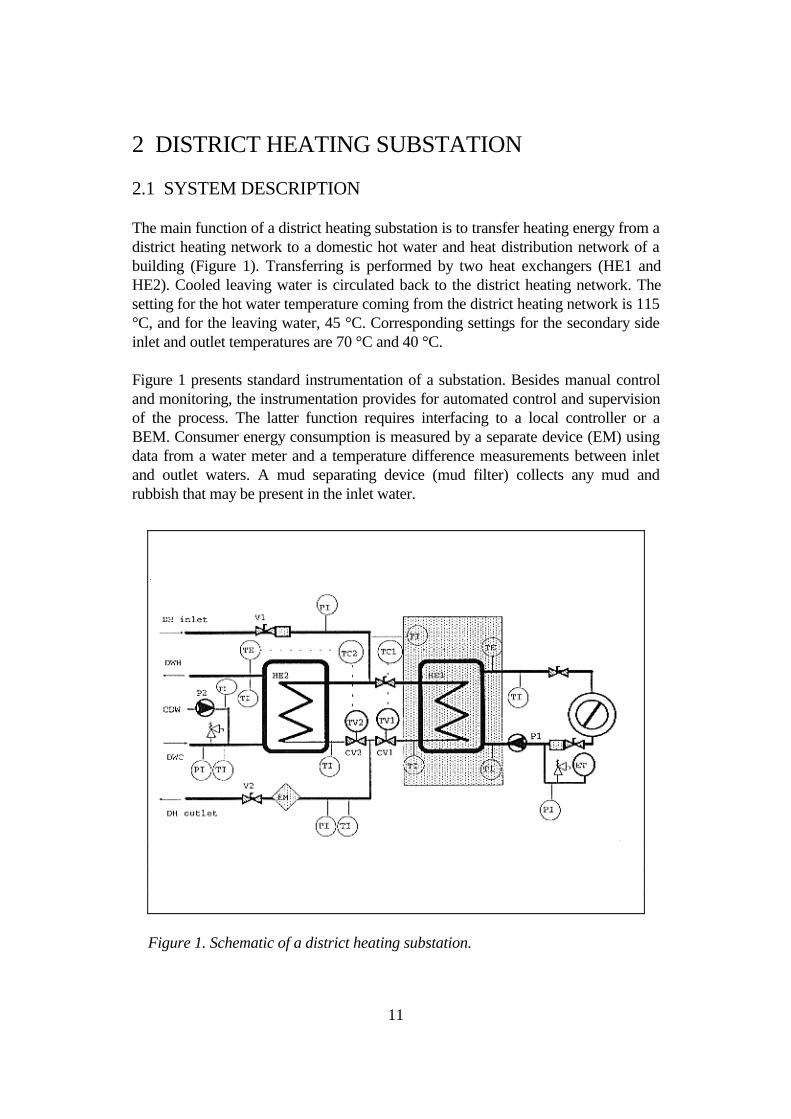
The main function of a district heating substation is to transfer heating energy from adistrict heating network to a domestic hot water and heat distribution network of abuilding (Figure 1). Transferring is performed by two heat exchangers (HE1 andHE2). Cooled leaving water is circulated back to the district heating network. Thesetting for the hot water temperature coming from the district heating network is 115°C, and for the leaving water, 45 °C. Corresponding settings for the secondary sideinlet and outlet temperatures are 70 °C and 40 °C.

Figure 1 presents standard instrumentation of a substation. Besides manual controland monitoring, the instrumentation provides for automated control and supervisionof the process. The latter function requires interfacing to a local controller or aBEM. Consumer energy consumption is measured by a separate device (EM) usingdata from a water meter and a temperature difference measurements between inletand outlet waters. A mud separating device (mud filter) collects any mud andrubbish that may be present in the inlet water.

Figure 1. Schematic of a district heating substation.

12

2.2 DOMESTIC HOT WATER

Domestic hot water temperature is continuously kept at 55 °C. Variations caused bychanging load conditions are minimized by a control circuit. This is rather difficultdue to the short time constant of the heat exchanger. The instrumentation of thecontrol circuit consists of a temperature sensor TE, a controller TC2 and a controlvalve TV2, which mixes cold and hot water. A water pump P2 runs day and night,recirculating the water through the domestic water network. Local pressure andtemperature instruments PI and TI enable monitoring of the cold water supply.

2.3 HEATING NETWORK

The heat distribution network consists of the components on the right of Figure 1.Besides the heat exchanger, the system includes a radiator network, a circulatingpump P1, an expansion tank ET, a pressure relief valve and a control circuit withtwo temperature sensors, a controller TC1 and a control valve TV1.

The expansion tank is necessary to smooth out the pressure and volume variations inthe water due to changing water temperature. Additional pressure relief is possibleby means of the pressure relief valve. If the water level of the radiators is low, theyare filled with water through a pipe (FI).

The heat supply through the radiator network is controlled by TC1 using an actuatorcombined with a control valve (TV1) and two measurements, one from the outdoorair and the other from the network inlet temperature. The control strategy differsfrom the control of the hot water. The set point of the water temperature depends onthe outdoor temperature. The measurement from the inlet water is required to keepthe outlet temperature at the desired level. Typically, changes in set point values andloads are slow. That is why temperature control of the heating water isuncomplicated.

2.4 TYPICAL FAULTS IN A SUBSTATION

According to Hyvärinen & Karjalainen (1993) the main effort in developing FDI-methods for a district heating substation should be directed to the components: heatexchangers, valves, controllers, actuators, sensors and pipes. Each of thesecomponents generates faults characteristic of the component, its function and thesurrounding process environment. However, similar components in similarfunctions give rise to faults which are peculiar to the component regardless of theprocess. Thus, the mentioned components have typical faults presented in Table 1. Adistrict heating substation consists of over one hundred components. Each of themmay have a fault. Emphasis is placed on the listed components because of their

13

assumed high failure rate and their significant role in the operation of the substation.

Table 1. Examples of typical faults found in components of a district heatingsubstation.

COMPONENT FAULTS

Heat exchanger - leakage - blockage - dirtiness

Valve - stuck or binding - failure open or close - leakage

Controller - drift - bias - hunting - faulty electronics - faulty computer program

Actuator - shaft seizure or binding - failure open or close - bent or disconnected linkage

Sensor - bias - drift - poor location

Pipes - clogging - leakage - faulty insulation

2.5 PROBLEMS IN FAULT DIAGNOSIS OF A SUBSTATION

The structure and operation of a district heating substation is straightforward.However, the environment contains several characteristic features, which makediagnosis difficult. One of them is a poor instrumentation level. Standardinstrumentation of a substation is designed only for control and local monitoringpurposes, not for automated fault diagnosis. Extra instrumentation means additionalcost, which is not acceptable to the consumers. If extra instrumentation is allowed, atmost it is one or two temperature sensors or corresponding low-cost instruments.The demand for economical solutions also means that diagnostic methods must be

14

included in local controllers or in BEMs. No separate diagnosis system, parallel toan existing controller or BEM, is allowed.

The consequences of insufficient instrumentation are clearly seen by monitoring thewater pressure of the district heating network. The pressure variation is totallyunpredictable and changes in the pressure directly effect every piece of equipment inthe primary side. Thus, without interfaced pressure measurements, which is anormal situation, modelling of the process is inaccurate and model-based faultdiagnosis is demanding.

Some of the typical faults in substation components are difficult to detect. One ofthem is internal leakage in the hot water heat exchanger. In such a failure, districtheating network water is mixed with domestic hot water. Measurable symptoms areminimal and operation of the process seems to be normal. But contamination of thehot water may cause health risks. Another typical fault is accumulation of dirt on theinner surfaces of the heat exchangers. The phenomenon occurs gradually, but canfinally cause blockages and a total breakdown of the equipment. Due to the abovementioned problems, these kinds of faults are very difficult to detect. This is thereason why the following FDI methods concentrate only on faults causing distinctand abrupt changes in the operation.

15

3 CLASSIFICATION OF FAULTS AS A METHODTO ELIMINATE PROBLEMS OF THRESHOLDADJUSTMENT

3.1 INTRODUCTION

A typical problem in fault detection is the threshold adjustment. Optimal thresholdadjustment is difficult to achieve, which is seen in practice as unreliable or unrobustoperation of diagnosis systems, i.e. false alarms or undetected faults. One possiblesolution to the problem is to classify detected faults in several hazard grades. Thebenefit is that alarm messages need not be sent too early, if the fault is insignificant.Thus, at least part of the false and unnecessary alarms can be neglected. This kind ofperformance classifier can operate as an independent fault detector and/or classifier,parallel to another fault detection method, or embedded in a diagnosis system. Themethod is appropriate for applications in which performance of the process is easilycategorized quantitatively and/or qualitatively. Typically it can be used as asupplement to a fault diagnosis system. The method is illustrated by classifyingfaults of sensory instruments. Further applications are presented in the followingchapters.

3.2 PROBLEMS OF THRESHOLD ADJUSTMENT

Every fault detector makes decisions based on some threshold or limit value.Thresholds may be set according to a-priori knowledge but usually they are set byutilizing measured data, gathered during normal operation of the process, and byapplying a statistical estimation procedure. Statistical estimation methods do notensure 100% probability and finite limits at the same time. Degradation or smallchanges in the process may also effect the probability limits and the thresholds(Pakanen 1992). Sometimes disturbances contain noise components, which are notconsistent with the assumed probability density functions. The effect is directly seenon threshold levels.

The proper level of an alarm may also be set by the user. But without goodknowledge this easily leads to intuitive adjustments. The result is non-sensitive oreven inoperative fault detection caused by too many false alarms and a frustrateduser. In addition, threshold adjustment also depends on performance requirementsset on the fault detection. If early detection is required the method and limits willdiffer from fault detection, that is executed over a longer time period. Also, a fault ofminimum magnitude needs more effort and different tools than a distinct and abruptchange in process operation.

16

3.3 INCREASING THE ROBUSTNESS OF FAULT DETECTION

Threshold adjustment is one way to increase the robustness of fault detection. Ifthreshold adjustment is reliable, it has a positive effect on overall fault diagnosis.One alternative for increasing robustness is to apply several independent methods,and thus utilize several threshold levels to detect the same fault. This is identical toincreasing analytical redundancy of the detection. If most methods indicate an alarmcondition, an actual fault is probable. Another alternative is to apply the user andhis/her knowledge in the decision of the possible fault. Then, the fault detection andneeded decisions are based on wider knowledge than a single threshold level. Butthe decisions and actions of the user must be based on real information of theprocess, not on intuition. Such a solution easily leads to an expert system or tointeractive fault tree reasoning (chapter 6).

Threshold adjustment of fault detection has received the attention of manyresearchers. For example, Halme et al. (1994) proposes a method based onqualitative reasoning and temporal constraints. Frank (1994) suggests thresholdadaption using fuzzy logic. Many of the presented methods are based on adaptivethresholds. Patton (1994) gives a survey of several techniques.

The approach presented in this paper differs from those above. The classificationconcept is based on the performance of the observed signals (Pakanen 1993). In thisscheme, fault size is defined according to its effect on process performance,especially on process output. Numerical values given to a performance measure orindex allows classification of faults into different hazard grades. This approach isconvenient when early detection is not the primary objective. In this scheme, thedecision of the fault grade requires monitoring of several limits. But there is no needto accurately adjust them because the hazard grade of the fault is known. Estimationof the hazard grade allows more thorough consideration of the right time of alarmmessages, decisions and actions are to be made. This makes it possible to prevent atleast some of the false and unnecessary alarms and still maintain sensitivity of faultdetection.

3.4 PERFORMANCE INDEX

A central idea in the classification concept is the performance index, denoted asJi(x), which is defined in the following way. Let W = w1,w2,...,wc be a finite set ofclasses, representing fault grades. A classifier finds the best category wi, i =1,2,3,...,c for the data, i.e., the most probable fault grade, by computing adiscriminant function Ji(x), where x is a vector-valued variable. The classifierassigns the feature vector x = (x1,x2,...,xd)

T to class wi if

17

Each feature component xj defines a quantitative or qualitative property typical ofthe fault grade. The performance index Ji(x) attaches one numeric or symbolic valuefor each feature component xj, which together specify a valid region for the faultgrade.

Equation 1 sets only a few requirements for Ji(x) and allows numerous ways torealize the function in practice. One alternative is to define Ji(x) as a logic functionwhich is consistent with the rule-based programming techniques. If all numeric orsymbolic values concerning one fault grade wi and one feature component xj areincluded in a set Si,j, then the performance index is easy to represent as

where number 1 denotes a value true and 0 a value not true. According to theequation 1, only one of the performance indices Ji(x), i=1,2,...,c can have the valuetrue each time.

The performance index can be set to any or all monitored signals of the process. Butprocess output is a natural alternative because targeted performance and allowablefluctuation of the output are usually defined during system design.

3.5 FEATURES

Each fault category contains features which are characteristic to the process and theapplication. Feature selection is based on a-priori knowledge of the observedprocess. Features can be quantitative or qualitative in character. A process with onecontinuous output y(t) might have features concerning the size of deviation, averagefrequency of fault appearance and duration of failure. Similarly, limits can be set forrequired minimum activity of y(t) during a prescribed time period, or tolerances ofdy/dt, i.e. derivative of y(t). A controlled process signal might provide features likemagnitude of overshoot, settling time and number or existence of overshoots. Thelast one represents an example of a qualitative feature.

3.6 PRACTICAL FAULT GRADES

In practice, the number of fault grades must limited to a few categories. If faults areclassified in three hazard grades, they would be: tolerable, conditionally tolerableand intolerable faults (Isermann 1984). A tolerable fault means that the operation of

( ) ( )i jJ > J , j i .x x ∀ ≠ (1)

i

j i, j

j i, jJ (x) =

1, if x S , j = 1,2, ,d

0, if x S , j = 1,2, ,d ,

∈ ∀∃ ∉

(2)

18

the process can continue but an indication of an exceptional situation is recorded.Process output is slightly changed but performance of the process is still satisfactory.It is not known whether the change in the operation is due to a disturbance or a fault.A conditionally tolerable fault requires a change in the operation. Clearly, a failurehas occurred and the operating time of the faulty process is limited. Performance ofthe output is somewhat degraded, which cannot be tolerated for a long time. Thefault is reported to the operator. If the fault is intolerable, the operation is stopped orradically changed, if possible and an alarm message is immediately sent to theoperator.

3.7 APPLICATION OF THE PERFORMANCE CLASSIFIER

The classification concept described above is not a conventional fault detectionmethod. The primary intent is to classify performance of the process. But when thesize of a fault is defined according to its effect on prescribed, measured signals ofthe process, then the confirmed hazard grade also helps in fault detection and faultsize evaluation. Figure 2 presents a case where the performance of the processoutput is measured using the procedure. The method operates independently as afault detector/classifier.

The performance classifier can also operate parallel to a conventional faultdiagnosis method. In this case, the procedure serves as a supplement to thediagnosis, because it is able to evaluate the size of the detected and isolated fault.This is a common objective of fault diagnosis, but it is rarely achieved in practice.Figure 3 illustrates a case where performance monitoring and fault classificationoperates parallel to a model-based fault detection system. The residual r(t) makes itpossible to indicate the type of the fault and its occurrence time while theperformance classifier reveals the size of the fault.

Figure 2. Performance monitoring and classificationof a process output as an independent operation.

19

A third alternative for using the performance classifier is embedded operation. Inthis case, the indexing procedure is hidden in a fault diagnosis system. Figures 4 and5 present an example of a pattern recognition system, which is applied in faultdiagnosis of input signals u(t). Recognition requires learning of fault features fromthe input signals. As shown in Figure 4, all extracted features are combined with aperformance measurement of the output y(t). Then, the classifier can link a fault toits effect on the process output, i.e., the fault grade. After the learning phase, faultsand their hazard grade in the input u(t) are directly detected and classified withoutthe performance classifier, as shown in Figure 5.

Figure 3. Parallel operation of a performanceclassifier and model-based fault detection.

Figure 4. Learning phase of a pattern recognitionsystem combined with a performance classifier.

20

3.8 AN EXAMPLE: FAULT DETECTION OF SENSORYINSTRUMENTS

System description

The following example concerns fault detection of sensory instruments of an HVACcontroller. Analog signals coming from the sensors are analyzed and possible faultsare detected using performance index methodology.

Sensors and their interface to a controller may contain several types of faults.Typical is a loose or broken contact or connector, which may cause a sudden andlarge change in the measurement signal of a resistive sensor. The phenomena can betemporary or irregularly repeated. A cold solderjoint or corrosion may change thescale and cause larger instabilities in the measurement. External inductive orcapacitive noise, which may be temporary or permanent, cumulates as noise ofvariable magnitude in the measurement. Aging or the temperature of thesurroundings are often the reason for drift in the measurement signal. The proposedmethod is planned to detect all these faults except the last one, which is usuallyfound during calibration of the measurement.

Features

The sensory instrument produces an analog signal which is continuously monitored.The signal is assumed to go through several tests, which extract certain features andtheir proportional magnitudes. The features together form a feature vector F. Thefollowing features described by feature variables are included:

Figure 5. Fault detection and classification of apattern recognition system with embeddedperformance indices.

21

Size of deviation (x1)duration of fault (x2)Average frequency of fault appearance (x3).

A definition of each feature is given later in this chapter. Thus, the feature vector ofthe faults is defined as F = (x1, x2, x3)

T. The problem is to partition the three-dimensional feature space into regions where all the points in one regioncorresponds to one fault grade. Similarly to fault grades, the regions of featurevariables are also qualified in three categories, which describe their magnitude orintensity. Although the feature category may have a qualitative name, the limits ofeach region will be specified quantitatively.

The size of deviation (x1) could be partitioned like the other features. However, thefollowing partition, which comes from natural behavior of the input signal, isapplied. In this scheme, the size of deviation includes three type of limits on bothsides of the signal. The closest limit is called the dynamical limit Ud which is givenas a result of signal prediction. The analog signal is first modelled with an ARMA-model, which combines both deterministic and stochastic features of the signal inone model. The model is identified during the normal operation period and thenapplied as a predictor. A k-step predictor is written as

At time t the above equation gives the predicted value of the real signal u(t+k),where k is the number of sampling periods. The dynamic limit of the signal isachieved when a probability limit is calculated for the prediction. For example,when the 95% probability limit is applied

where fk is a coefficient of a polynomial related to the ARMA-model.

The saturation limit Us describes the extreme values of the sensory signal when theoutput quantity of the controller gets its physically realizable maximum or minimumvalue. Similarly to the dynamic limits, the saturation limits locate both sides of thesignal as an upper and lower limit. The dynamic limits are usually closer to the realsignal than the saturation limits. For analog measurement signals, the saturation-limits are prescribed using a-priori information or a test sequence of the process.

The absolute limit Ua is the extreme value of the sensory instrument where analogmeasurements give sensible results. The absolute limit may be located far away fromthe other limits. The absolute limits are defined from the characteristics of the

( ) ( ) ( ) u t + k / t = - c gi=1

m

i

i=0

m-1

iu t+k-i / t-i + u t-i .∑ ∑ (3)

( )d 12

22

k-12

U = u t + k / t 1.96 1 + f + f + + f ± σ (4)

22

sensory instruments and an A/D-converter of the controller. The absolute limit andthe preceding limits are normally related as

The duration of the fault (x2) combined with the size of the deviation effectivelyindicates the character of the fault. A small deviation of a short period may befiltered out, but larger and longer ones can cause damage to the system. The durationof the fault is defined as the time period during which the signal exceeds one of theabove specified limits during consecutive sampling instants.

In order to relate the duration of the fault to the corresponding hazard grades, onemust use both a-priori information and experimental results. Abnormal deviation ofthe analog measurement signal has an effect on the output or the main function ofthe system. When noise of variable variance and duration in the input is added theircommon effect on the output can be categorized in the three hazard gradespreviously mentioned. These kinds of experiments could be performed by themanufacturer of the controller.

The average frequency of the fault appearance (x3) is also a meaningful feature. Ararely appearing short deviation in the measurement, exceeding the low limit hardlycauses any trouble to the system. It can be assumed to be cumulative random noiseand is easy to filter out. If it appears frequently, the situation is different. In this case,it may refer to a loose or broken connection. The average frequency of faultappearance, and the size and duration of the deviation are closely related to eachother. That is why determination of frequency limits for different hazard grades mustbe performed together with the other limits.

An illustration of classification

Tables 2, 3 and 4 illustrate a case where three type of faults are classified accordingto the features and their values. The tables illustrate the way how the results ofclassification could be presented. They are not based on any real data ormeasurements. The intensities of each feature in the tables are describedqualitatively but in practice all categories must also be defined numerically. They areprescribed during the preliminary tests. The tables form a three-dimensional systemthat defines the class of the fault in all grades of intensities of the features.When the fault is classified the system can choose the necessary actions to be takenafter fault detection. A tolerable fault is perhaps not a good reason to send an alarmmessage to the user, but the time of appearance and the class of the fault may beworth recording. A conditionally tolerable fault may require some actions to betaken in addition to the alarm message, and an intolerable fault could stop or changethe operation of the process.

a s d d s aU > U > U > U(t) > U > U > Umax max max min min min (5)

23

3.9 SUMMARY

Classifying faults into several hazard grades gives new possibilities of avoiding falsealarms, because fault detection is not based on one threshold level. The three hazardgrades: tolerable, conditionally tolerable and intolerable fault permit more thoroughestimation of the effect of the fault on the process and the right time to send analarm message. The classification concept is based on the performance index, whichcan be set to any or all monitored signals of the process. The procedure based onperformance indexing can operate independently as a fault detector/classifier,parallel to another fault detection method, or embedded in a diagnosis system.

24

Table 2. Classification of a fault according to the three types of features. Frequencyof the fault appearance low.

Size of deviation Fault of very short duration

Fault of shortduration

Fault of notableduration

Exceedingabsolute limit

conditionallytolerable

intolerable intolerable

Exceedingsaturation limit

tolerable conditionallytolerable

intolerable

Exceedingdynamical limit

tolerable tolerable conditionallytolerable

Table 3. Classification of a fault according to the three types of features. Frequencyof the fault appearance moderate.





intolerable intolerable intolerable





tolerable conditionallytolerable

intolerable

Table 4. Classification of a fault according to the three types of features. Frequencyof the fault appearance high.











25

4 FAULT DETECTION METHOD FOR SUB-STATION PRIMARY FLOW ROUTE ANDCONTROL VALVE

4.1 INTRODUCTION

In this section, a method is described that was developed as a part of technicalwork carried out for developing fault detection methods (Hyvärinen 1994a,Hyvärinen 1994b) for two typical heat production units: district heatingsubdistribution system (Hyvärinen & Karjalainen 1993) and oil burner (Hyvärinenet al. 1993). The method is based on a simple physical first principles staticprocess model and on the use of analytical redundancy (Frank 1990) of the systemunder consideration. In other words, the redundancy contained in the staticrelationships among the system inputs and measured outputs is exploited for faultdetection. The procedure of evaluation of the redundancy given by a mathematicalmodel of some system equations can be roughly divided into two steps: generationof residuals, and decision and isolation of the faults. Here the residuals aregenerated based on static parallel model approach, and on parameter estimationapproach in which the consistency of the mathematical equations of the system ischecked by using actual measurements. Because of the static process model, directredundancy relations can be used. The decision is based on a simple threshold.The cause of the fault can be diagnosed based on parameter estimates of theprocess.

The main emphasis in the development work has been on simplicity and onpractical rather than on theoretical aspects of the method. The reason for this isthat it is assumed that in the near future field level application specific controllerswill be capable of simple diagnostic tasks but with limited computationalrecources only. For example, the computational speed, numerical andmeasurement accuracy, and amount of memory are limited for practical and, in theend of the day, for economical reasons.

Practical application of a fault detection method requires that the model structureis known and its parameters can be estimated reliably. Also it is required that thethreshold values and parameter deviations from their nominal values for faultdetection can be determined before the method is taken into use. For thesepurposes and especially for processes with linear control valve least squaresestimation algorithms provide a good methodology and applying the method isquite straightforward. For processes with exponential control valve also theunlinearity must be modelled before the required model parameters and thresholdvalues can be solved.

26

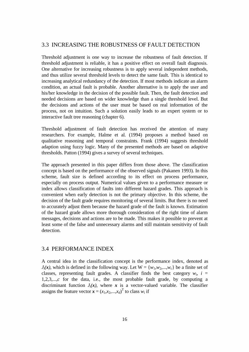
4.2 OUTLINE OF THE PROCESS AND THE METHOD

The simplified process can be approximated to consist of control valve and a flowroute the flow of which the control valve affects (Figure 6). The control valverepresents a varying flow resistance. The flow route consists of a pipeline andother components, and it represents a constant flow resistance. The process isconnected to an outside network which generates the pressure difference over theprocess. In an oil burner the pressure is generated with an oil pump in the burner, and in a district heating subdistribution system the distribution network can beseen as a constant pressure source.

dppressure

difference from the outside network

constant flow resistance

varyingflow resistanceq

mass flow

uactual control

signal

outside network

Figure 6. Electrical circuit analogy of the flow route and control valve.

The control valve can be described as a flow resistance the value of which changesas a function of actual control signal. The structure of the function of the varyingflow resistance is usually known for each specific valve and it is typicallycharacterised either by exponential or linear valve equation. In case of water or oilas media the process is fast and it can be considered to be in a steady statecondition all the time. The process dynamics need not to be considered.

The basic idea of the method is to use a process model that relates the threevariables: pressure difference dp, mass flow q, and actual control signal u. Processfaults can then be detected either by calculating one of the process variables fromthe others, and comparing the calculated value to actual measured value, or byestimating the process model parameters and comparing them to nominal values.The threshold values and nominal parameter values are estimated from a nonfaulty process condition.

27

4.3 FAULT DETECTION METHOD

Process model

The flow and pressure equations of the simplified subprocess are

2 2vq = kv * dp (6)

dp = dp + dps v (7)

s s2dp = Z * q (8)

where Zs is constant flow resistance of the heat exchanger and pipelineThe dependency of the valve kv-value from the shaft position in general can bemodelled with the following equation

( )kv kv g uc= * (9)

where the function g(u) describes the valve unlinearity.

Applying equations 7, 8 and 9 to 6 the following equation is obtained

2c2 2

c2

s2 2q = kv * g(u ) * dp - kv * Z * g(u ) * q (10)

and further when arranging for g(u)2

g(u) =q

kv * dp - kv * Z * q2

2

c2

c2

s2 (11)

Taking a derivative of 10 with respect to u and supposing that dp does not changeas a function of u, the following equation is obtained.

( ) ( ) ( ) ( ) ( )∂∂

∂∂

q

ukv dp g u g u kv g u g u Z q kv g u Z

q

uc c s c s

22 2 2 2 2

2

2 2= ′ − ′ −* * * * * * * * * * * *

(12)If the valve unlinearity is characterised with the following equation

( ) ( )′ =g u C g u* (13)

the equation 12 can the be presented as below

( ) ( ) ( )∂∂

∂∂

q

ukv dp C g u kv C g u Z q kv g u Z

q

uc c s c s

22 2 2 2 2 2 2

2

2 2= − −* * * * * * * * * * * *

(14)

28

By applying equation 11 to 14 and solving it with respect to dp*d(q2)/du thefollowing is obtained

dpq

uC q dp C Z qs* * * * * * *

∂∂

22 2 42 2= − (15)

Now, equations 10 and 15 form the equation set that models the subprocess. Incase of a linear valve is utilised instead of an unlinear one, equation 10 aloneforms the model. The underlined parts represent signals that are measured andcalculated from process signals and the other parts represent model parametersthat are estimated during tuning and operation phase.

Unlinear valves that fulfils the requirement of equation 13 are, for exampleexponential valves characterised with following equations.

( )g u ene u= * C=ne (16)

( )g unp

u

= −

−1

100

100( )

Cnp

= −

ln 1

100 (17)

where np and ne are manufacturer specific parameters used to describe theunlinearity.

Finally the subprocess model is

Table 5. The process quantities that have to be measured.

quantity computation/ measurement unit meaningdp PI1-PI2 kPa pressure differenceq FI m3/h water volumetric flowu TV % valve shaft position

Often, the valve position is not measured and only the control signal value isknown. This causes extra work during the tuning of the method because the valveshaft position as a function of control signal must be modelled. The control signalvalue from the controller can not be used in place of shaft position because thecontrol signal changes stepwise and position rampwise and there is a differencebetween these two signals. The valve position must be used instead.

The measured values (Table 5) must be instantaneous values and they may not befiltered or averaged in any way. The sampling time does not play any role. It can

( )

( )q

kv g u dp

kv Z g u

c

c s

22 2

2 21=

+

* *

* (18)

29

be of varying length and chosen arbitrarily. The signals (underlined terms) inequation 10, however, can be filtered with any linear filter. They can, for example,be cumulated over some time interval.

Method description

Process faults can be detected either by using a model output error (Figure 7) orparameter deviations from their nominal values (Figure 8). The model output erroris the residual between the model output, q2 , given by equation 18, and the actualmeasured value. If the parameter deviations are used for fault detection theparameters of equations 10 and 15 are estimated periodically and compared tothose estimated during tuning phase.

process model

comparisonto threshold

threshold valuesfrom tuning

phase

+

-

uvalve shaft

position

pressure differencedp

flowq

valveunlinearity

( )2

process measurements

Process para-meters from tuning phase

test quantity

symptom

tuning information

Figure 7. Block diagram of the output error method.

Process para-meters from tuning phase

estimation ofprocess model

parameters

comparisonto threshold

threshold valuesfrom tuning

phase

+

-

uvalve shaft

position

pressure differencedp

flowq

valveunlinearity

( )2

process measurements

test quantitiessymptoms

tuning information

Figure 8. Block diagram of the parameter error method.

30

The square of flow given by equation 18 is compared to the square of the flowmeasured and calculated from the process. The value of the function g(u) iscalculated using equation 20 or 21. The parameter values of equations 10 and 15and the threshold values for fault detection are estimated during the tuning phaseand fixed during the operation phase.

When parameter deviations are used for fault detection, the parameters of theprocess model (equation 10) are estimated periodically and the results arecompared to values estimated during the tuning phase. The parameters of themodel describing valve unlinearity (equation 15) are estimated only during tuningphase and are fixed during normal operation period.

If the subprocess is linear i.e. there is no such a component that causes someunlinear feature like the unlinear valve does, then the parameters can be estimatedon-line instead of periodical estimation.

The method is tuned following the steps below1. Measuring the tuning data2. Prehandling of the measurement data3. Parameter and threshold value estimation.

It is important that the input signals to the process vary in a large enough area i.e.the input signals must be exciting enough. It would be best if each of the normaloperation point could be measured during the tuning phase for a long enough time.For practical reasons this is usually not possible and the tuning must be done withless information. The process is assumed to be in non-faulty condition during themeasurement of tuning data. The method is “taught” the non-faulty operation ofthe process during tuning phase. When, at the operation phase, the measuredprocess operation deviates from the taught (modelled) operation, it can beassumed that there is a fault in the process.

In the DHS, the valve control signal can be varied freely. One has to take care thatno harm is caused to the other parts of the process or user. For example, thedomestic hot water temperature may not rise too high if the water is used duringthe tuning period. The control signal should be varied between 0 % and 100 % ifpossible. The changes should be slow enough so that the valve actuator and realposition of the valve have enough time to travel to each operation point.

The pressure difference over the subprocess can not be affected by the operator.The pressure difference varies according to the heating load of the external districtheating network. At a minimum, one should get measurement data for onepressure difference value over all the valve position values.

During the tuning and operation phases only unfiltered raw data are utilised.Outliers should be removed if possible. Also those operation points where theprocess has clearly operated erroneously should be removed. For example, in a

31

near open and close situation the process may saturate due to erroneous tuning ofthe actuator causing erroneous information of the process operation.

Figure 9. Process characteristic curves and calculation of partial derivativeof q2 with respect to valve shaft position.

In equation 15 the output signal (regressed variable) is the partial derivative of thesquare of flow with respect to the valve position. Solving this on-line frommeasurements is sensitive to measurement noise which causes the result to beunreliable. For this reason the partial derivative is calculated off-line from acharacteristic curve of the process (Figure 9).

Figure 10. Process characteristic curves of figure 8 plotted as a surface (mesh-plot). The flow value remains in zero at dp value 1.6 because there has not beenany measurements at that value. In reality the value of q increases continuoslywith value of dp.

A characteristic curve is formed from the process (Figures 8 and 10), in which thevalve position u is on the x-axis and square of the flow on the y-axis. The differentcurves in Figure 8 are isoclines having different values of pressure difference. The

32

partial derivative is calculated for each discretized position of u on each isoclinecurve using the following equation.

∂∂

+ −2q

u=

q (u du) - q (u du)

2 * du

2 2(19)

Parameter and threshold value estimation

Equation 15 can be represented in the following form

y x a x a e= ∗ + ∗ +1 1 2 2 (20)

where y= dpq

u

∂∂

2

, x1 =2*q2*dp, and x2 =2*q4 are signals a1 = C and a2 = -C*Z

and e is assumed to be zero-mean white Gaussian noise the variance of which isλ2

The parameter values a1 ja a2 are estimated using least squares method(Söderström 1989). Using parameter a1 the parameter describing the valveunlinearity ne or np can be solved.

Because the partial derivative of square of the flow is solved from a characteristiccurve the parameters must be estimated off-line. Furthermore, the estimationresult is better if the averages are removed before the estimation. This, too,requires an off-line estimation method to be used.

Equation 10 can be represented in the following form

y x b x b e= ∗ + ∗ +1 1 2 2 (21)

where y=q2, x1 =g(u)2*dp, and x2 =g(u)2 * q2 are signals b1 and b2 areparameters, with covariance of P and e is assumed to be a zero-mean whiteGaussian noise the variance of which is λ2

The parameter values b1, b2, their covariance matrix P, and the estimate of thevariance l2 of noise e, are estimated using the least squares method. In this case,too, the result is better if the averages are removed from the signals beforeestimation.

It is not possible to choose a threshold value for fault detection that gives 0 %false alarm rate. The thresholds are chosen in such a way that an alarm does notnecessarily mean a fault but may be caused by normal measurement noise, too.After an alarm occurs, it must be decided if the alarm is caused by a fault.

Fault detection method output is the residual between subprocess model andcorresponding measurements. As a threshold for this residual a value calculatedfrom the variance l2 of the noise e is used. The threshold values are chosen in thesame way as in case of oil burner.

33

Applying the method requires reasoning in two ways. Firstly, the way thethreshold values are selected does not guarantee a 0% false alarm rate and thusthe decision of the fault situation must be done for example using a classifierpresented in chapter 3. Secondly, the method produces a set of test quantities thechanges of which indicate some faults in the process. The test quantities that canbe used in addition to the residual, are the parameters a1, a2 , b1 and b2.

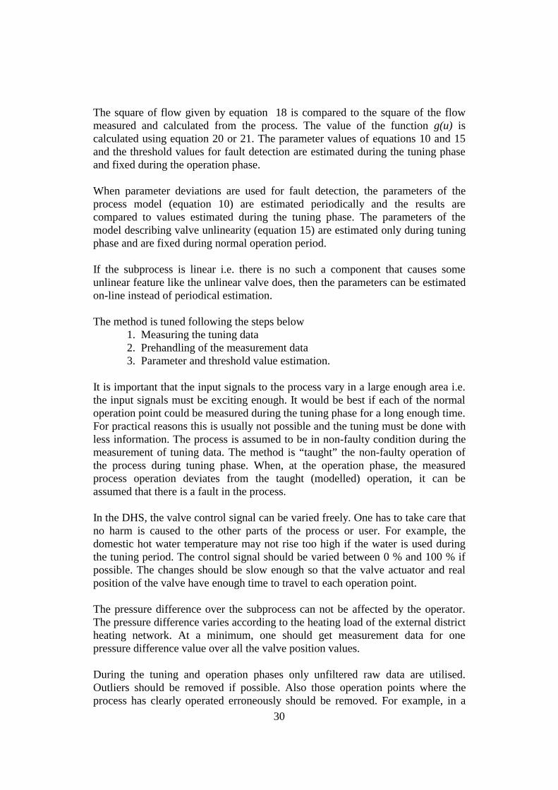
Figure 11. DHS Tuning data.

4.4 RESULTS

The tests shown in Figure 11 were done with the subprocess to tune the modelparameters. The measurements were used to build the characteristic curve, and forparameter estimation. In the upper half of the figure both the flow (solid line) andthe pressure difference (dashed line) are presented. In the lower half of the figurethe valve shaft position is presented.

Figure 12 shows the simulated square of the flow (dashed line), the correspondingvalue calculated from the measurements (solid line), and the confidence limits.Only those operation points are included where the valve position has been in theinterval of [5% - 80%]. The simulation model of equations 16 and 18 has beenused and parameters shown in Table 6 were obtained. The error of the simulationis shown in Figure 13.

34

Figure 12. Simulation of q2. Simulation done with tuning data.

Figure 13. Error of the simulation using tuning phase data.

The results of applying the method to a non-faulty process are shown in Figures14 and 15. In 14 simulated (solid line) and measured (dashed line) q2 arepresented. In Figure 15, the model residual (i.e. the error between measured andsimulated process output) and its thresholds are presented. In the testing phase,only those measurements where the actual control signal remained in an intervalof [5% - 70 %] were taken into account. The other measurement values wereconsidered to be out of the valid area of the method.

35

Table 6. Parameter estimates obtained from tuning phase.

Equation 20b1

b2

1.0e-3*0.35280.1054

λ2 0.0046P 1.0e-9*0.65 0.67

0.67 0.71ne 0.0558

Figure 14. Simulation of q2 using testing phase data.

36

Figure 15. Residual of simulation of q2. The residual is the difference betweenmeasured process value and respective simulated one.

4.5 CONCLUSIONS

The method operates well and can be utilised in practical applications according totest results for a non-faulty process. Fault simulations and evaluation of thesensitivity to different faults must be carried out before practical application. Themethod utilises well known techniques and for that reason is easy to implement.Calculationally the method is light. The heaviest tasks in calculation are theparameter estimation and, in case of an unlinear valve, the calculation of anexponential term.

The method copes with a specific unlinear processes. The unlinearity assumed istypical in district heating systems and in HVAC applications. The unlinearitycauses the performance of the method, if measured in terms of output errorwhiteness, to decrease, and the complexity of the method to increase. With a lin-ear valve the method gives better results is less complex, and needs less calcula-tions and memory.

The method does not give 0% false alarm rate but requires an additional classifierto make the decision whether the alarm is caused by a fault or not. The Methodproduces several test quantities, which all can be used in diagnosing the fault or inimproving the fault detection. By combining the information from different testquantities the method gives relatively fault selective information of the processoperation.

37

5 FAULT DETECTION METHOD OF A HEATEXCHANGER

5.1 INTRODUCTION

The aim of this paper is to describe one approach to detecting a leak in a heatexchanger. Leakage is chosen as an example because it is one of the mostcommon faults and has an obvious effect on the operation of the heat exchanger.This method is based on continuously evaluating the heat power differencebetween the primary and the secondary side of the heat exchanger. The method isbased on both steady state and dynamic models.

5.2 DESCRIPTION OF THE METHOD

Process

The process being examined is limited to heat exchangers and temperature sensorsof district heating subdistribution system (Figure 1). Therefore the methoddepicted, which is based on the heat power balance, is limited to the diagnostics offaults occurring in heat exchangers and temperature sensors. This method isapplicable to the operation of heat exchangers for heating and for domestic hotwater heat exchangers. Here, only one heat exchanger is examined. The operationof the district heating subdistribution system is shown by Hyvärinen &Karjalainen (1993).

Faults detected by the method

The heat power balance method for a heat exchanger calls for flow measurementswhich are generally not installed in district heating subdistribution system (Figure1). These flow measurements are substituted by other components' such as controlvalves' and pumps' characteristic curve methods or using some more economicalmeasuring method than flow measurement, such as measuring the pressuredifference over a constant flow resistance. This way the number of faults foundby the method increases. Using only the exchanger's heat balance method, thefollowing faults can be identified:

a) An internal or external leak in the heat exchanger.b) The malfunction of a temperature sensor.

38

This method does not isolate a faulty component or direct the user to correctivesteps; instead, it only detects the fault or sends the information to the reasoningsystem installed in the building's upper level automation system.

Calculation model of the method

This method is based on the continual observance of the heat exchanger'scalculated static heat power balance (Q2 = hQ1). The heat exchanger's primary

flow transfers heat through the heat surface to the secondary flow. Part of this heatis transferred through the heat exchanger's casing into the environment. This heatloss is taken into account in a heat transfer efficiency h (equation 22). The heattransfer efficiency is supposed to be constant all the time, which is not exactlycorrect. Nevertheless, the heat loss is insignificantly small in an insulated heatexchanger. The heat exchanger's primary and secondary heat power is calculatedusing measured or calculated flows from other models and with the help ofmeasured temperatures (equations 23 and 24). The operating point of the heatexchanger under varying conditions causes errors in the stady state calculationmodel. It has been attempted to reduce the error by changing the static model ofthe heat power balance to an dynamic ARX-model (equation 25). Figure 16 showsthe principles of the calculation model of the method.

Q = f(q ,T)1 m

qm,1

T12

qm,2

T22

T21

Q = f(q ,T)2 m

K * e -dt

tau*s + 1Q = f(Q )1 2

+

-e

Measurements

T11

Dynamic model

Residual

Static models

Figure 16. The calculation model of the heat power balance method. Subindex 1corresponds to the heat exchanger's primary side, and 2 to the secondary side.

The dynamic model is used to calculate the primary side's heat power from thesecondary side's heat power while taking into account the varying conditions ofthe heat exchanger and the slow response of the measuring devices. The heat lossinto the environment is included in the dynamic ARX-model's parameters a and b(equation 25), which in the tuning phase of the method are determined from theheat powers of the primary and secondary side which are calculated with the static

39

model by means of the least squares method. In the steady state conditions theconstant heat transfer efficiency is determined from the dynamic model'sparameters (η = (1-a)/b). Based on experience of the measurements the heattransfer efficiency can also be over one because of inaccurate of the measuringdevices and the calculated fluid properties. The determined heat transfer efficiencyindicates also how successful the parameter's tuning has been. For example, thetypical heat transfer efficiency varies between 0,9 - 1,0. In continuouslymonitoring the operation of a heat exchanger, the relative error of the heat powerof the calculated primary side and the heat power determined from themeasurement quantities are compared (equation 26).

Static models:

Q Q1 21=η

(22)

Q q c Tm p1 1 1 1= , , ∆ (23)

Q q c Tm p2 2 2 2= , , ∆ (24)

Dynamic models (k = sample time):

Q k aQ k bQ k1 1 21( ) ( ) ( )= − + (25)

e kQ k Q k

Q k( )

( ) ( )

( )= −1 1

1

(26)

The heat power balance error e (residual), is thus the relative error of the primaryside's heat power calculated using two different approaches, and in the continuousstate of an unimpaired process it is approximately zero. In a fault situation theerror in the heat power balance diverges more from zero than the predefined alarmlimits, and the user is accordingly warned of the fault.

Measurements

Figure 1 shows typical measurements of a district heating subdistribution system.The heat exchanger's power balance method needs additional primary andsecondary flow measurements. If the flow measurements are replaced by thecalculation models of other components (i.e., control valve and pump) the methodcan examine the operation of more components than before.

Although the flows are replaced by the calculation models of other components,the flows must also be measured at the tuning phase. This way the flowscalculated from the model can be compared to the actual flows and the heatexchanger's dynamic computation model can be tuned using the actual flows for

40

calculating the heat powers. The flow can be measured in the tuning phase byusing ultrasonic measurements, for example.

The sample measurement data should be an instantaneous value. The test intervalshould be sufficiently frequent (< 5 seconds) if the model is to performsatisfactorily in the changing conditions of the process. It does not matter howfrequently samples are taken while observing continuous operations.

5.3 THRESHOLD CALCULATION

It is not possible to define a threshold for the faulty process using analyticalmethods to attain a zero per cent rate of false warnings. The thresholds for theprocess must be selected in such a way that when a quantity describing amalfunction exceeds the limit selected, this does not necessarily imply amalfunctioning of the process, since instead the exceeding may be due tomeasurement noise or to some other statistical phenomena. After the threshold hasbeen exceeded, it must be deduced how significant the exceeding is and whetherthe exceeding has caused by the faulty process. This is determined by a reasoningsystem.

The threshold for the error of the heat power balance method is calculated in thetuning phase of the method, while the dynamic model's parameters a and b aredefined using the least squares method. The threshold th is determined by meansof equation 27 as the product of the deviation η of the relative heat power balanceerror (Figure 16) and the selected coefficient kr.

th kr= ∗λ (27)

While the heat power balance is at its normal distribution, the coefficient kr can beused, for example, to calculate the thresholds of the following heat power balanceerror's reliability limits:

kr = 1,65 -> 90% of the calculated values within the thresholdskr = 1,96 -> 95% of the calculated values within the thresholds andkr = 2,58 -> 99% of the calculated values within the thresholds.

5.4 TUNING OF THE METHOD

In the phase when the method is tuned, the parameters a and b which take intoaccount the dynamics of the calculation model, are determined as well as thethreshold th. The tuning of the parameters is most successful when the heatexchanger's loading is varied within a wide operating range using large step-likechanges of secondary side flow. In practice, this is not always possible. For

41

example, in small buildings the load of a heat exchanger for domestic hot watercan be changed easily over a wide operating range, but in large buildings it is moredifficult to make sufficiently large changes in the load. In this case, it is a goodidea to do the tuning during a time when the load varies a good deal owing tonormal consumption.

If the threshold is tuned by using the same measuring data as for tuningparameters, it must be taken into consideration that changes in the operating pointwill increase the threshold. If the threshold is tuned in the steady state conditions,the calculated threshold is error limit of measurement noise. The changes in theoperating point of heat exchanger will increase the threshold. The greater thechanges made to the operating point, and the more frequent they are, the higherthe threshold is. Tuning the threshold changes should be done in the normalprocess having characteristics of normal use so the threshold can be set as low aspossible. In tuning the threshold, it is necessary to use different data than for theparameters in the calculation model if the loading changes in the process arevalues from normal operation.

Tuning and commissioning according to the method are done by phases asfollows: 1. Measuring the temperatures and flows and recording data if necessary.2. Carrying out loading changes and calculation of the parameters of the dynamic

model.3. Calculation of the threshold value from the measurement data stored previously

or from separately measured data.4. Setting the parameters and threshold for the calculation model.5. Starting the on-line calculation model.

5.5 UPPER LEVEL REASONING

If the threshold is exceeded, the cause must be deduced and it must be decided ifan alarm signalling this error should be sent. The reasoning system can beimplemented in the building's so-called upper level automation system, in which afinal assessment can be made of the seriousness of the exceeding the thresholdvalues for the error of the heat power balance and the necessity of registering analarm. If a reasoning system connected to the upper-level automation system is notavailable, this should be taken into account in determining the alarm limit. In thiscase a larger coefficient must generally be used than the one which was used todetermine the threshold in Section 5.3.

When the process's components are operating correctly, the threshold is exceededowing to rapid changes in the heat exchanger's operating point or momentaryrough measurement and data transmission errors. The reasoning system can bebased, for example, on an assessment of the magnitude, duration and frequency of

42

occurrence of the exceeding of the threshold of the calculation value indicating afault, as shows in Chapter 3. The seriousness of the exceeding of the threshold foran error in the heat power balance can be classified, for example, according toTables 7 and 8 on the basis of the duration and the magnitude of the exceeding orthe frequency of occurrence and magnitude of the exeeding. Reasoning accordingto Table 8 is facilitated if, say, a signal commanding a control valve is used as anaid in the reasoning. A signal commanding the control valve can be used todeduce whether the process is in a state of change or not. When the signalcommanding the control valve changes, it does not make sense to use inferencerules for the frequency of occurrence of the exceeding.

In Tables 7 and 8 a model-related calculation error means a calculation error dueto a program error or to inaccurate tuning or a calculation error due to states ofchange within the process; a measurement error means an error in measurement ordata transmission.

Table 7. An example of classifying the exceeding of the threshold and deduction ofthe seriousness of the exceeding on the basis of the duration and magnitude of theexceeding (Chapter 3).

Duration and valueof exceeding

Exceeding < 10sec

Exceeding < 10min

Exceeding > 10min

Large (4*threshold)

Model-relatedcalculation erroror measurementerror or processfault -> alarm

Model-relatedcalculation erroror process fault -> alarm


Medium(2*threshold)

Model-relatedcalculation erroror measurementerror -> noalarm

Model-relatedcalculation erroror process fault -> duration over10 sec -> alarm


Small (1*threshold)

Model-relatedcalculation erroror measurementerror -> noalarm

Model-relatedcalculation erroror measurementerror -> no alarm

Model-relatedcalculation erroror process fault -> duration over10 min -> alarm

43

Table 8. An example of classification of the exceeding of the threshold anddeduction of the seriousness of the exceeding on the basis of the frequency ofoccurrence and magnitude of the exceeding. A signal commanding the controlvalve is used as an auxiliary quantity in the reasoning.

Exceedingfrequency andmagnitude

Seldom (< 10times / 10 minand controlunchanged)

Quite frequently(< 60 times / 10min and controlunchanged)

Frequently (> 60 times / 10min and controlunchanged)

Large(4*threshold)

Model-relatedcalculation erroror measurementerror or processfault -> alarm


Model-relatedcalculation erroror process fault-> alarm

Medium(2*threshold)




Small(1*threshold)




Tables 7 and 8 show examples of inference rules whose alarm limits are suitablemainly for a heat exchanger for domestic hot water. In the case of a heatexchanger for heating, the alarm limits can be stricter, at least as far as themagnitude of the exeeding is concerned, since the changes in load due to theprocess's dynamics do not cause an error in the calculation model to the sameextent as they do with a heat exchanger for domestic hot water. Alarm limits ofthe reasoning system cannot be determined analytically, but instead they must beset to the correct level on a trial and error basis.

5.6 RESULT EXAMPLES

Presented in the following are results of operational tests made with the heatpower balance method for a heat exchanger in laboratory conditions. The processexamined is shown in Figure 17. The process is subprocess shown in Figure 1except for the flow measurements of the primary and secondary side and inaddition it shows the pipe describing a leak in the heat exchanger. The heatexchanger in the process is a soldered plate heat exchanger having a nominalpower of 30 kW. The demonstrated leak in the heat exchanger occurs between thedistrict heating (DH) inlet fit of the flow primary side and the outlet fit of the flowof the secondary side. The direction of the leak is from the primary side to thesecondary side.

44

Figure 17. The demonstration process of the method.

Tuning example

The calculation model of the power balance method for a heat exchanger is tunedaccording to the phases shown in Section 5.4. Figure 18 shows an example oftuning of the parameters and tuning data, i.e., the heat powers calculated from themeasured values. Figure 19 shows an example of tuning the threshold. Thethreshold is determined with a 95% reliability limit (kr =1.96).

time

heat

pow

er (

kW)

0

5

10

15

20

25

10:40:59 10:41:39 10:42:19 10:42:59 10:43:39 10:44:19 10:44:59 10:45:39

0

0.2

0.4

0.6

0.8

1pa

ram

eter

Parameter a

Parameter b

Secondary side heat power

Primary side heat power

Figure 18. Tuning of parameters a and b of the dynamic calculation modelaccording to the method as well as the heat powers of the primary and secondaryside which were used as tuning data. The heat powers have been calculated frommeasured values. The values of the parameters at the end of the tuning are a =

45

0,981 and b = 0,020.

time

heat

pow

er (

kW)

0

2

4

6

8

10

12

14

16

18

11:01:53 11:03:14 11:04:35 11:05:56 11:07:17 11:08:38 11:09:59 11:11:20

0

0.05

0.1

0.15

0.2

0.25

0.3

0.35

0.4

0.45

resi

dual

& tr

esho

ldPrimary side heat power


Treshold value th

Abs. residual |e|

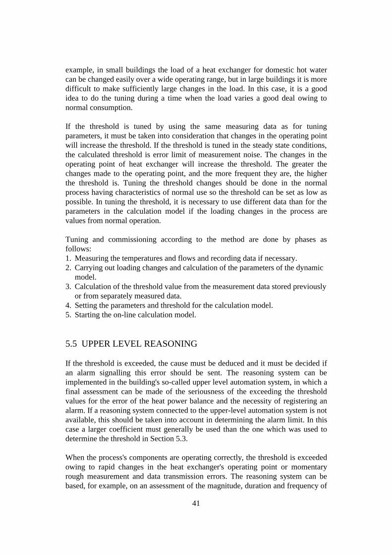
Figure 19. Tuning of the threshold according to the method. The tuning data usedare the residual, which is the relative error of the primary side's heat powerdetermined from the measured values and calculated with the dynamic model. Avalue of 0,128 (95% reliability limit) was obtained as the threshold.

Operation example

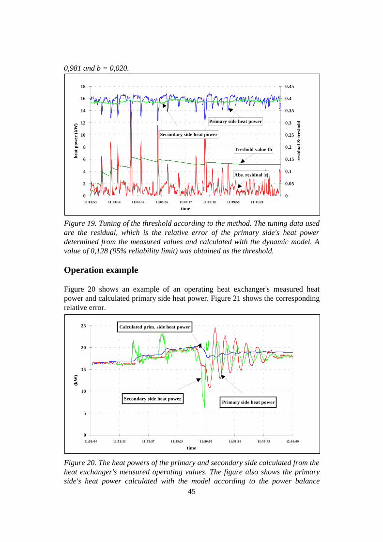
Figure 20 shows an example of an operating heat exchanger's measured heatpower and calculated primary side heat power. Figure 21 shows the correspondingrelative error.

time

(kW

)

0

5

10

15

20

25

11:51:04 11:52:31 11:53:57 11:55:24 11:56:50 11:58:16 11:59:43 12:01:09

Calculated prim. side heat power

Secondary side heat powerPrimary side heat power

Figure 20. The heat powers of the primary and secondary side calculated from theheat exchanger's measured operating values. The figure also shows the primaryside's heat power calculated with the model according to the power balance

46

method.

time

resi

dual

-0.3

-0.2

-0.1

0

0.1

0.2

0.3

11:51:04 11:52:31 11:53:57 11:55:24 11:56:50 11:58:16 11:59:43 12:01:09

Treshold

Treshold

Figure 21. The relative error e of a heat exchanger's measured and calculatedprimary side heat power with the load period according to Figure 20.

Figure 22 shows an example of a leaking heat exchanger's measured heat powersas well as the calculated primary side heat power. The leak from the heatexchanger's primary side to the secondary side was an average of about 20% of theprimary flow and about 15 % of the secondary flow. Figure 23 shows thecorresponding relative error.

time

(kW

)

15

17

19

21

23

25

27

13:12:00 13:12:43 13:13:26 13:14:10 13:14:53 13:15:36 13:16:19 13:17:02 13:17:46

Primary side heat power


Calculated prim. side heat power

Figure 22. The primary and secondary side heat powers calculated from a heatexchanger's measured operating values as well as the primary side heat power

47

calculated with the model according to the power balance method.

time

resi

dual

-0.3

-0.2

-0.1

0

0.1

0.2

0.3

13:12:00 13:12:43 13:13:26 13:14:10 13:14:53 13:15:36 13:16:19 13:17:02 13:17:46

Treshold

Treshold

Figure 23. The relative error e of a heat exchanger's measured and calculatedprimary side heat power with the load period according to Figure 22.

5.7 CONCLUSIONS

In developing a heat power balance method for a heat exchanger, the assumptionwas that the flow measurements required for the method can be replaced bycomputational models of other components such as the control valve and thepump. The developed calculation model of control valve (Chapter 4) can beutilised by using the calculated flow instead of the measured primary side flow.For a pump, it is also possible to determine the characteristic curve model of theflow as a function of the electrical power drawn by the motor. Measurement of theelectrical power should nevertheless be highly precise, which means that themeasurement is as expensive or even more expensive than measurement of theflow. In addition, a characteristic curve model of the pump cannot be utilised in adistrict heating subdistribution system other than in determining the flow of aheating-related heat exchanger's secondary side. Accordingly, notwith standing theoriginal objective, it was not possible to avoid so-called added instrumentation inimplementing the method.

It is probably cheapest to implement the problematic secondary side flow of theheat exchanger by measuring the pressure difference of the flow across a constantresistance. For example, in a heat exchanger the resistance of the flow is nearly aconstant. The pressure difference of the flow across a heat exchanger also makes itpossible to deduce whether the heat exchanger is affected by a large amount ofgrime or blocking. Measurement of the pressure difference of the primary sideflow across several components is also used in the calculation model for a control

48

valve (Chapter 4). In this case, if the heat exchanger has a large amount of grimeor is severely blocked, this is also detected on its primary side, providing that themodel for a control valve is in use.

In the development phase of the method, all the analyses were done on a solderedplate heat exchanger. The method nevertheless functions in a similar manner in alltypes of exchangers, because the principle of the process is the same. On the basisof the simulations and laboratory measurements made, the method acts as a meansof detecting leaks occurring in a heat exchanger. Furthermore, on the basis ofsimulations, a fault in the temperature sensor can also be detected. In thelaboratory measurements the leakage point in the heat exchanger was not varied;rather, the leak was always between the heat exchanger's inlet fit of the districtheating flow and outlet fit of the secondary side flow or out from either of thefittings.

When the process is in the static state, the method can be used to detect relativelysmall leaks. In the laboratory measurements the smaller leaks detected with themethod were about 5 % of the measured primary side flow. A problem isnevertheless the errors which the process's dynamics cause in the computationalquantity indicating a fault, since this quantity raises the final alarm limits.Accordingly, the amount of measurement data available for the reasoning systemand the way in which the reasoning system is implemented largely determine howsmall the leaks can be in order to be detected with the method. On the basis ofanalyses made in the laboratory, it can be observed that a simplified dynamiccomputational model according to the method does not function sufficiently wellin order to manage the changes in load of a heat exchanger in the desired manner.The problem is mainly in tuning the model to provide sufficient sensitivity as wellas the complicated dynamic behaviour of the process, which is comprised of a heatexchanger and control devices. This aspect is dealt with in the source (Ahonen &Kuismin 1993), among others. Thus, the above-presented method is best suited tomonitoring a process which remains in the static state for long periods and inwhich the changes in load are slow.

Another problem occurring in a heat exchanger, and one which in practice isperhaps more troublesome than a leak, is the accumulation of grime on the heattransfer surfaces. The above-presented method, which has been supplemented bymeasurements of the pressure difference of the primary and secondary side flowsacross the heat exchanger, has not been tested and thus there is no first-handexperience of its suitability for detecting the accumulation of grime. The grimethat builds up on the heat transfer surfaces of heat exchangers is often very finelydivided. The grime presumably does not have a very significant effect on thefrictional resistance of the flow but, on the other hand, it has a considerablygreater effect on the heat transfer ability of the heat surfaces. Thus, theaccumulation of grime on the heat transfer surfaces could be defined better bymeans of the heat transfer coefficient of the heat surfaces or with some othercorresponding quantity than with the flow resistance. The approach in question

49

calls for a detailed knowledge of the construction of a heat exchanger and precisetuning of the computational models so that they operate well with the object towhich they are applied. An approach of this type is used in the fault diagnosismethod of a static model of a heat exchanger, which is described by Blomberg etal. (1992).

50

6 INTERACTIVE FAULT TREE REASONING

6.1 INTRODUCTION

Fault diagnosis of small HVAC-controllers needs special attention, because of theirlimited memory, computing capacity and demand for cost-effective implementation.Sophisticated methods may be unreliable and multiply the need for memory andcomputing capacity of the controller. This paper suggests a method called interactivefault tree reasoning. The method activates the user and the controller to co-operation, which simplifies the fault localization procedures and reduces the needfor extra instrumentation. The method is a natural way to implement a reliable, cost-effective diagnostic system of a district heating substation with moderate additionalhardware and software requirements.

6.2 FAULTS LOCALIZED BY AN EXPERT USER

Fault localization is a problem of HVAC-controllers and other local buildingautomation devices. A typical controller gives an alarm signal or outputs a code orshort message to a display unit when a possible fault is detected. Fault detection isusually based on limit or trend monitoring instead of more sophisticated methods(Sprecher 1992). However, an alarm signal or message rarely identifies the real faultlocation, confusing an inexperienced user. Such a system needs an expert user, whoknows the process and can make measurements and search for the location of thefault. A separate reasoning method to point out the actual fault and its hazard gradeis not a common feature of such devices.

This is also true for controllers of district heating substations. The level ofinstrumentation, limited memory and computing capacity of the controllers togetherwith insufficient knowledge of process characteristics and demands for cost-effective implementation do not support development of complicated faultlocalization methods. Thus, due to the lack of practical procedures, the actual faultcan only be found by an expert user or experienced serviceman.

6.3 FAULTS LOCALIZED BY AN EXPERT CONTROLLER

The other extreme is achieved if the controller contains a real-time embedded expertsystem. After fault detection the cause of the problem is automatically identified.Only the fault and its location and hazard grade are reported to the user. In this case,the user need not be an expert. All knowledge including facts and problem-solvingrules are stored in the data base. Unfortunately, an embedded expert system needs atenfold or even hundredfold memory capacity compared with the original processcontrol program. Technically it is possible to increase the memory capacity. Also,the need of extra computing capacity to maintain both process control and expert

51

system functions can be satisfied. However, the situation reveals a problem oftenencountered in applying fault detection and localization methods. The memory andcomputing capacity of the diagnostics exceeds many times those of the mainfunction of the system. Still they are needed only a few times during the life cycle ofthe device. In addition, the system inevitably needs extra instrumentation in order tosimplify the diagnostic procedures. All these features increase the costs and/ordecrease the reliability of the system.

6.4 AN INTERMEDIATE FORM OF THE TWO METHODS

The above methods represent two extreme approaches of reasoning, where the roleand expertness of the controller and the user are opposite (Figure 24). A practicalmethod can probably be found somewhere between these two extremes. A goodmethod allows cost effective implementation of the controller with an ordinary levelof instrumentation. The method must be easy to apply and lead to reliable operationof the main functions and diagnostics.

A practical reasoning method for a district heating substation is suggested, whichbenefits the co-operation of an inexperienced user and non-expert controller. Themethod is an intermediate approach of the above two methods and later referred toas interactive fault tree reasoning. In this method, the dialoque is controlled and thereasoning is supervised by the HVAC-controller and it follows a fault treeprocedure, which is a conventional fault localization method (Pau 1981). The basicidea is to activate the user to interactive co-operation with the controller. This is notjust answering questions but reading instruments, reporting symptoms andperforming manual control actions supervised by the controller. Thus, the size of thenecessary knowledge-base is reduced and the reasoning rules can be implementedwith an ordinary programming language. Symptom-oriented fault tree reasoningwith logical reduction rules (Visuri 1986, Lautala et al. 1989) make procedures shortand selective. Interactivity and the special role of the user also minimizes the needfor extra instrumentation and multiplied memory and computing capacity. Adrawback is the reduction in flexibility compared with the expert system approachand the need of a versatile user interface.

6.5 INSTRUMENTATION REQUIREMENTS

Implementation of the interactive fault tree reasoning only requires ordinary processinstrumentation, local and interfaced. Sometimes it is possible to reduce thecomplexity of the fault tree procedure by adding a new instrument. If the instrumentis not essential to the main process, a cost effective choice may be to add a localinstrument without any connection to the controller. There may appear faults that aredifficult to detect and locate with ordinary methods and instrumentation. In such acase, visible symptoms recognized by the user may be crucially important forlocalization of the fault.

52

Because the user is inexperienced and not familiar with the process, it may benecessary to label the instruments the user is going to touch or check. The samesymbols are output in the instructions of the controller.

Because the controller does not include an expert system, the extra memory andcomputing capacity are moderate. However, the new method needs a good userinterface that outputs clear messages and instructions to the user. Interactivity alsorequires fluent data inputting capabilities. Although technical prerequisites for suchuser interfaces have been available for a long time, practical, cost effective solutionsare products of recent years.

6.6 DIAGNOSTIC TESTS

Fault evaluation and localization will be more straightforward if the controllerperforms diagnostic tests (Pakanen 1996). A diagnostic test is a sequence of controlactions, measurements and mathematical algorithms that check the condition of onemachine or piece of equipment. The test may be accomplished by the controlleralone or assisted by the user. Because the instrumentation supervised by thecontroller is limited, co-operation of the user can simplify the test procedures. Testscan be performed without significantly disturbing the main functions of the process.

6.7 MORE SPECIFIC FAULT DETECTION

Alarm signals and messages of commercial controllers are results of relativelysimple fault detection methods, which may refer to several faults. However, thecontroller is able to collect data and perform many kinds of algorithms andcalculations that are not complex and time consuming, such as calculation ofstatistical parameters, fault frequencies, maximum and characteristic quantities(Isermann 1984). The information may help to design more specific fault detectionmethods. A detection method decreasing the number of alternative choices alsosimplifies the fault localization.

6.8 SELECTION OF THE FAULT TREE PROCEDURE

A single fault can easily cause several different alarm signals to be sent to thedisplay. This is a serious problem in supervising large processes. Attempts havebeen made to solve the problem with alarm analysis and logical reduction rules(Visuri 1986, Lautala et al. 1989). They sort the alarm signals and allow onlyrelevant ones to propagate to the user. The same rules are also useful in smallersystems with interactive fault tree reasoning. But now these rules are applied to sortthe right fault tree procedure to be followed. When several alarms originate fromone fault, the essential alarm signal can be solved with the aid of timing and the

53

logical relationship of the alarms. The chosen alarm signal points to a fault tree thatreveals the most probable origin of the fault. If the logic cannot discern the rightalarm from a wrong one, the user may have to go through several fault trees.

6.9 DEALING WITH UNCERTAIN INFORMATION

While reporting the tasks to the controller, the user makes decisions and performsreasoning in his mind, which reduces the handling of uncertain information. Becauseall of the information is not numerical, the controller must have a procedure forhandling uncertain information. This is also a general aspect of a good userinterface. On occasions when qualitative information must be handled, it can bepresented with fuzzy variables or certainty factors. The rules may be similar toexpert systems, but presented with ordinary programming language.

6.10 APPLICABILITY

The above method is appropriate for small, uncomplicated applications, wherereliable fault diagnosis would require heavy instrumentation and/or complicatedmethods without the aid of the user. Although the user is not an experiencedserviceman, it is helpful if he is familiar with the basic operation of the process andknows the names and locations of the equipment. Such a situation is common inresidential HVAC-systems. Occupants who constantly observe the behavior ofheating or air conditioning easily recognize possible changes in the process.

6.11 THE METHOD APPLIED IN A DISTRICT HEATINGSUBSTATION

A district heating substation (Figure 1) is a proper system for interactive fault treereasoning. Ordinary instrumentation interfaced to the controller is not versatileenough to ensure fault detection and localization with usual methods and therequirement of cost-effective implementation does not allow for extrainstrumentation. The problems of fault detection and localization are due to thenonlinear processes and unstable characteristics of the district heating supply.However, the interfaced and local instrumentation makes it possible to successfullyapply interactive fault tree reasoning. User tasks are easy to perform, because all theequipment and instrumentation of the substation are installed in one compact space.Table 9 presents typical user tasks when the method is applied in a district heatingsubstation.

54

Table 9. Typical user tasks applicable in a fault localization procedure.

- close or open a valve- check the position of a valve- check the condition of a fuse- check the position of a switch- read a thermometer- read a pressure gauge

- check the condition of a safety valve- check the operating condition of a pump- manual on-off control of a pump- check if a heat exchanger has an outside leak

Table 10. Typical faults located using the interactive fault tree reasoning.

- mud filter dirty- temperature of the district heat water is low- flow rate of the district heat water is low- heat exchanger of the heating system is leaking- control valve of the heating system out of order- temperature measurement of the heating water out of order- set point temperature curve of the heating water needs adjustment- circulating pump of the heating water out of order- outdoor temperature measurement out of order- temperature control of the heating water out of order- temperature measurement of the domestic water out of order- control valve of the domestic water out of order- temperature control of the domestic water out of order- set point temperature of the domestic water needs adjustment- circulating pump of the domestic water out of order- heat exchanger of the domestic water is leaking- pipe blockage in the heat exchanger of the domestic water- pressure level of the heating pipe is low

55

Figure 25 represents a flowchart of a fault tree procedure starting from a watertemperature alarm. The procedure shares tasks between the user and the controller.Actions taken by the user are presented using darkened boxes. The user inputs therequested information or certifies a performed task. The interactivity requires thatthe controller informs the user of all decisions and achieved results. The flowchartdoes not present all details of the communication. The total number of symptom-oriented fault trees is ten to fifteen, which is enough to the most common faults to belocated. Table 10 presents typical faults that are possible to locate with the method.

The fault tree procedures may take several forms, depending on instrumentation,user tasks and the characteristic of the faults. One must optimize the costs, usertasks, reliability and complexity of the fault diagnosis procedure. The interactivecommunication must not be too long and complex or the user will get bored. It maybe better to point out several possible faults rather than make the procedure too long.Another way to shorten the procedure is to avoid a too detailed specification of thefault. There are also situations, where it is not possible to solve and locate the fault.In such a case the fault may be temporary or the symptoms are non-visible and/ornon-measurable.

6.12 CONCLUSIONS

Interactive fault tree reasoning represents a competitive choice for fault localizationof a district heating substation. In spite of non-linearities and variation in processcharacteristics, the method is applicable for reliable localization of many kinds offaults. The method can be implemented without adding extra instrumentation. Extrahardware and software requirements are also moderate. These features make themethod a cost-effective and practical solution for district heating substations andother small HVAC-processes.

56

Figure 24. Interactive fault tree reasoning as a combination of two extremeapproaches.

57

Figure 25. A flowchart of the fault localization procedure. The procedure finds afault when the symptom is high heating water temperature. Darkened boxes refers toactions taken by the user.

58

7 DETECTING BLOCKAGE OF A MUDSEPARATING DEVICE USING A STATISTICALTEST

7.1 INTRODUCTION

A new method for detecting blockage of a mud separating device or mud filter ispresented, which is based on an uncomplicated statistical test. The fault detectionmethod is suggested to be installed in a building energy management system (BEM)or a temperature controller of a district heating substation. A starting point was tofind a solution which is practical and directly applicable in existing automationsystems. The outcome was therefore an uncomplicated statistical method. Themethod utilizes the normal instrumentation of a district heating substation. Onlysome additional software is needed for a controller or a BEM to be able to apply themethod. No further instrumentation is required.

For a fault to be detected, the process needs to be in good condition at least for theidentification period during which the characteristic features of normal operation arerecorded. Apart from these data, the method does not require any additionalinformation from the user. The method can thus be programmed to be used in acontroller with a reduced user interface.

The following description concentrates exclusively on mud filter diagnosis, but themethod can also be used to monitoring of a control valve, for example.

7.2 THE MUD SEPARATING DEVICE AND SYMPTOMS OFBLOCKING

In a district heating substation, the mud filter collects all the mud and rubbish thatmay be present in the heating water. It prevents them from entering the controlvalves and heat exchangers and thus allows the other parts of the substation tooperate undisturbed. The mud filter may operate for years without getting blocked.In such cases, the servicing intervals are relatively long. The possible blocks in themud filter, which cause symptoms in the operation of the substation, are often aconsequence of a local fault or disorder in the district heating network.

A blocked mud filter gives various symptoms. Owing to the block, not enough heatis transmitted into the domestic hot water, and the hot water temperature thereforetends to drop. The return water also has a lower than normal temperature. Becausethe temperature is inadequate, the control valves usually open abnormally into anearly or fully open position.

59

7.3 MONITORING OPERATION AND SYMPTOMSOF THE MUD FILTER

It is possible to detect blocking of a mud filter by observing the above symptoms. Tobe able to detect a fault, one must be aware of the normal temperatures fluctuationsand valve opening patterns. The fault detection method to be described belowcollects information from a normally operating process during an identificationperiod and uses this as reference data in detecting faults. The duration of theidentification period and the amount of information must be chosen in such a waythat the observed signals are persistently existing and that the amount of informationcollected is statistically sufficient. While monitoring system operation to detect apossible fault, the diagnostic system starts a "reference period" every now and then.The data collected during this period are analyzed and compared to the datacollected previously during an identification period. The emerging residual includesinformation on a possible fault. For the data to be reliable, however, it must bepossible to decrease the effect of disturbances and noise from the residual signalbefore any decision is made concerning the possible fault. This can be achieved bymeans of statistical testing.

7.4 STATISTICAL TESTING

Statistical testing and fault diagnosis

Statistical testing is part of the fault detection procedure in most diagnostic methods(Isermann 1984, Gertler 1988, Pau 1981). If the residual is structured (Patton 1994),it is possible to apply direct parallel testing, multivariate testing or sequentiallikelihood ratio testing. In the present case, the data consist of scalar signals, towhich univariate probability distributions and statistical tests can be applied. Onealternative would be to apply sequential tests to detect changes in means asBasseville (1988), but their use does not involve any essential benefits. Reliance onconventional and well-known procedures is useful from the viewpoint of thesystems designer, who is probably only familiar with the basic methods. This is apracmatic aspect, sometimes pointed out by automation manufacturers.

Test of means

Consider first how the expected values of hot water temperature can be tested. Thevalues measured for the signal are recorded at regular intervals during the identi-fication and reference periods. The results obtained during the identification periodgive an estimated mean, which is written as m1. According to the null hypothesis ofthe test, the mean m2, measured later during the reference period is identical to thatmeasured during the identification:

60

According to the alternative hypothesis:

In a failure, the mean is expected to be higher than normal. The test result showswhether the mean has changed significantly. The estimators of the mean are

where x1i and x2i are single measurements. The difference between the estimatorsX1-X2, on the other hand, is the estimator of the difference m1-m2. Assuming thatthe samples are mutually independent, the variance of the difference between themeans is written as

where s1 and s2 are the standard deviations of the measurements X1 and X2. Since s1and s2 are unknown in practice, they can be estimated by using the sample variances:

The actual test parameter t is thus

which is distributed approximately as N(0,1) when the null hypothesis is valid andthe sample sizes n1 and n2 are large.

0 1 2H : = .µ µ (28)

1 1 2H : > .µ µ (29)

11 i=1

n

1i 2

2 i=1

n

2iX = 1

nx X

nx

1 2

, = 1

,∑ ∑ (30)

( ) ( ) ( )21 2

21

22

12

1

22

2D X - X = D X + D X =

n +

n ,

σ σ (31)

( )21

1 i=1

n2

1i 1s = 1

n -1x - X

1

∑ (32)

( )22

2 i=1

n2

2i 2s = 1

n -1x - X

2

.∑ (33)

t = X - X

s

n +

s

n

,1 2

21

1

22

2

(34)

61

The null hypothesis is rejected at a 5 % significance level if

The limit value of the test parameter is obtained at a 5 % significance level of thenormal distribution N(0,1).

Test of relative proportions

The mean value test does not necessarily give reliable information on mud filterblocking, if the loading is increased for a long period or permanently. The blockingof the mud filter causes a change in the valve opening. This is seen as an increasingnumber of positions, in which the valve is fully open. So, the relative time for thefully open position is longer than normally and can be determined with a one-sidedstatistical test. The fully open position can be measured with a limit switch orapplying driving time of the actuator.

The testing of relative proportions is usually accomplished by using a binomialdistribution. But when the sample size is large, a normal distribution may becomemore appropriate. This is due to the fact that a binomial distribution approachesnormal distribution when the sample size is increasing. A necessity is that, theoriginal relative proportion must be nearly 0.5. In practice, this presents no problem.Another benefit of the normal distribution are the uncomplicated coefficients forlarge sample sizes, contrary to the the binomial coefficients.

It is assumed that parameter p=P(A) is the unknown probability of the event A. Theevent A refers to the relative proportion of fully open valve positions after a blockingof the mud filter. The fully open position refers to positions involving angles largerthan the given opening angle. The valve opening angle or the stem position ismeasured at regular sampling intervals for a predefined period. Parameter p iscompared to the given probability p0, which represents the probability in a normalsituation and is measured during the identification period. Hence, the normal andfaulty situations can be presented in terms of the following hypotheses.

The random variable x represents the frequency of occurrence of event A in a sampleof n events, of which it is known that

t > 1.645 . (35)

0 0

1 0

H : p = p

H : p > p . (36)

62

A random variable with a known binomial distribution has

The indicators corresponding to the relative frequency P=x/n of event A are

in which case the test parameter z with a nearly N(0,1) distribution is

A situation accordant with the null hypothesis is considered to be rejected at a 5 %significance level if

7.5 MEASUREMENTS

Measurements with an emulator

The data for the statistical testing were gathered using two different methods. Someof the measurement data come from laboratory tests performed with the VTT emula-tor system. The operation of the emulator was set to resemble the hot water plant ofa district heating substation, including a control valve with a control circuit, a heatexchanger and a manual valve simulating the mud filter of a district heating subs-tation. Persistent load variations were generated with a combination of a slow sinewave and a white noise signal. The system has been described in more detail byLaitila et al. (1992).

The measurements are from four different phases. At first, the identification phasewas started, during which the data of a normally operating system was recorded.After that, the position of the manual valve was changed to make the pressure diffe-rential across the valve greater than normal. This corresponds to a situation wherethe mud filter is partly blocked. After these settings, the measurements of the firstreference period were made. Then the pressure differential across the manual valvewas set to be even greater, and the same measurements were repeated. The

x Bin(n, p)_ (37)

Ex = np

D x = np(1 - p) .2

(38)

E( P ) = p

D ( P ) = p(1 - p)

n ,2

(39)

z = x - np

n p (1 - p ) .0

0 0 (40)

z > 1.645 . (41)

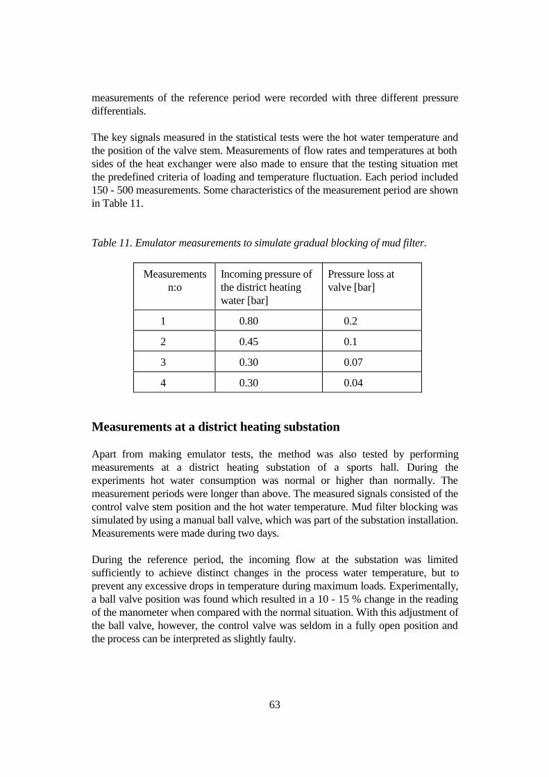
63

measurements of the reference period were recorded with three different pressuredifferentials.

The key signals measured in the statistical tests were the hot water temperature andthe position of the valve stem. Measurements of flow rates and temperatures at bothsides of the heat exchanger were also made to ensure that the testing situation metthe predefined criteria of loading and temperature fluctuation. Each period included150 - 500 measurements. Some characteristics of the measurement period are shownin Table 11.

Table 11. Emulator measurements to simulate gradual blocking of mud filter.

Measurements n:o

Incoming pressure ofthe district heatingwater [bar]

Pressure loss atvalve [bar]

1 0.80 0.2

2 0.45 0.1

3 0.30 0.07

4 0.30 0.04

Measurements at a district heating substation

Apart from making emulator tests, the method was also tested by performingmeasurements at a district heating substation of a sports hall. During theexperiments hot water consumption was normal or higher than normally. Themeasurement periods were longer than above. The measured signals consisted of thecontrol valve stem position and the hot water temperature. Mud filter blocking wassimulated by using a manual ball valve, which was part of the substation installation.Measurements were made during two days.

During the reference period, the incoming flow at the substation was limitedsufficiently to achieve distinct changes in the process water temperature, but toprevent any excessive drops in temperature during maximum loads. Experimentally,a ball valve position was found which resulted in a 10 - 15 % change in the readingof the manometer when compared with the normal situation. With this adjustment ofthe ball valve, however, the control valve was seldom in a fully open position andthe process can be interpreted as slightly faulty.

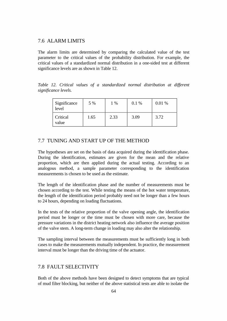
64

7.6 ALARM LIMITS

The alarm limits are determined by comparing the calculated value of the testparameter to the critical values of the probability distribution. For example, thecritical values of a standardized normal distribution in a one-sided test at differentsignificance levels are as shown in Table 12.

Table 12. Critical values of a standardized normal distribution at differentsignificance levels.

Significancelevel

5 % 1 % 0.1 % 0.01 %

Criticalvalue

1.65 2.33 3.09 3.72

7.7 TUNING AND START UP OF THE METHOD

The hypotheses are set on the basis of data acquired during the identification phase.During the identification, estimates are given for the mean and the relativeproportion, which are then applied during the actual testing. According to ananalogous method, a sample parameter corresponding to the identificationmeasurements is chosen to be used as the estimate.

The length of the identification phase and the number of measurements must bechosen according to the test. While testing the means of the hot water temperature,the length of the identification period probably need not be longer than a few hoursto 24 hours, depending on loading fluctuations.

In the tests of the relative proportion of the valve opening angle, the identificationperiod must be longer or the time must be chosen with more care, because thepressure variations in the district heating network also influence the average positionof the valve stem. A long-term change in loading may also alter the relationship.

The sampling interval between the measurements must be sufficiently long in bothcases to make the measurements mutually independent. In practice, the measurementinterval must be longer than the driving time of the actuator.

7.8 FAULT SELECTIVITY

Both of the above methods have been designed to detect symptoms that are typicalof mud filter blocking, but neither of the above statistical tests are able to isolate the

65

fault exclusively. If the pressure or temperature of the district heating network isabnormal relative to the loading, both tests may trigger an alarm. The same is alsotrue of faults in the hot water controller, which causes changes in the operation.Separate fault diagnosis and reasoning methods are needed for testing the operationof both district heating network and hot water controller, to allow differentiationbetween blocking of the mud filter and other faults.

7.9 TEST RESULTS

The above statistical test results suggest that the hypothesis h0 should be rejected ifthe value of the test parameter is higher than 1.65. This corresponds to a 5 % signifi-cance level. If the test parameter is higher than 2.33, a situation accordant withhypothesis h1 is probable at a 1 % significance level.

Tables 13 - 16 show the test results for both the test of means and the test of relativeproportions when data measured in the emulator experiment and at the districtheating substation were used.

Both the test of means and the test of relative proportions applied to the emulatorexperiments clearly imply that the hypothesis h0 should be rejected. Theidentification data shown in Table 14 consist of the results of measurement period 3,to minimize the pressure difference between the measurement periods. In this case,too, the tests yield results parallel to those shown in Table 13, but with slightly lowernumerical values.

Table 13. The results of the test of means applied to data measured in the emulatorexperiment. The results shown on the first line were obtained by using measurementperiod 1 (Table 1) as the identification data, while measurement period 3 was usedfor the results shown on the second line. Measurement period 4 was used as thereference material in both cases.

Value oftestparameter

Variancein identi-ficationdata

Variancein refe-rence data

Mean ofidenti-ficationdata

Mean ofreference data

8.04 11.28 46.74 39.48 34.49

4.49 30.73 46.74 37.71 34.49

66

Table 14. The results of the test of relative proportions applied to data measured inthe emulator experiment. The results on the first line were obtained by usingmeasurement period 1 (Table 1) as the identification data, while measurementperiod 3 was used for the results presented on the second line. Measurement period4 was used as the reference material in both cases.

Value of testparameter

Relative propor-tion, identi-fication data

Relative propor-tion, referencedata

7.19 0.51 0.80

4.26 0.52 0.69

Table 15. The results of the test of means applied to data measured at thesubstation. The results shown on the first line were calculated for a reference datasample of 100 measurements, while the results shown on the second line werecalculated for a sample of 30 measurements.

Value oftestparameter

Variancein identi-ficationdata

Variance inrefe-rence data

Mean ofidenti-ficationdata

Mean ofreference data

2.54 0.97 0.51 53.64 53.39

2.27 0.97 0.87 53.64 53.22

Table 16. The results of the test of relative proportions applied to data measured atthe substation. The results shown on the first line were calculated for a referencedata sample of 100 measurements, while the results shown on the second line werecalculated for a sample of 30 measurements.

Value of testparameter

Relative propor-tion, identi-fication data

Relative propor-tion, referencedata

2.19 0.44 0.55

1.38 0.44 0.57

The test results of the substation measurements are not so conclusive as those of theemulator experiment. Most of the test parameter values suggest the rejection of

67

hypothesis h0, but the numerical values of the test parameters only reach the 5 %significance level. The uncertainty is further increased by the test parameter value1.38 obtained in the test of relative proportions, which suggests that the nullhypothesis is still valid. This result was obtained using a smaller sample size.

7.10 CONCLUSIONS

On the basis of the experiment, the process water test of means and the valve stemposition test of relative proportions appear to be relatively good indicators of mudfilter blocking. For the detection to be reliable, however, the blocking must causemeasurable changes in the signals. The dimensioning of district heating substationsand the quality of loading vary. The test must be designed to take into account thesedifferences, for there may be differences in mud filter symptoms in even mutuallysimilar conditions.

Since the methods are able to detect blocking of the mud filter, but unable to isolateselectively the fault caused by it, they are best suited to be used in combination withanother or some other diagnostic methods. The actual fault should then be isolatedby reasoning.

In practice, both tests can be easily integrated with the software of the substationcontrol instrument or the controlling system. The procedure for detecting a fault issimple. The need for memory and data processing capacity is small. Nor is anyadditional instrumentation needed at the substation.

68

REFERENCES

Ahonen, M. & Kuismin, J. 1993. Experiments for a heat exchanger with a leakage.Working paper AN25/SF/310393/1.0, IEA Annex 25, Tokio 14. - 16.4 1993. 8 p.

Basseville, M. 1988. Detecting changes in signals and systems - A survey.Automatica, vol. 24, no. 3, pp. 309 - 326.

Blomberg, P. et al. 1992. Fault detection of district heating subdistribution system.First trial to detect a leakage in a heat exchanger. Working paperAN25/SF/161092/1.0, IEA Annex 25. Royal Institute of Technology (KTH,Sweden) and Technical Research Center of Finland, Laboratory of Heating andVentilation. 27 p.

Gertler, J. J. 1988. Survey of Model-Based Failure Detection and Isolation inComplex Plants, IEEE Control Systems Magazine, December 1988, pp. 3 - 11.

Frank, P. 1990. Fault diagnosis in dynamic systems using analytical and knowledgebased redundancy - A survey and some new results. Automatica, vol. 26, no. 3, pp.459 - 474.

Frank, P. M. 1994. Application of fuzzy logic to process supervision and faultdiagnosis. In: IFAC Symposium on Fault Detection, Supervision and Safety forTechnical Processes - SAFEPROCESS, Espoo, Finland, 13 - 16 June 1994. HelsinkiUniversity of Technology. Pp. 531 - 538.

Halme, A., Visala, A., Selkäinaho, J. & Manninen, J. 1994. Fault detection by usingprocess functional states and temporal logic nets. In: IFAC Symposium on FaultDetection, Supervision and Safety for Technical Processes - SAFEPROCESS,Espoo, Finland, 13 - 16 June 1994. Helsinki University of Technology. Pp. 189 -194.

Hyvärinen, J. 1994a. Fault detection method for district heating substation controlvalve based on static and physical model. Working paper AN25/FI/110494/1.0, IEAAnnex 25, Boston, 11. - 13.4.1994. 19 p.

Hyvärinen, J. 1994b. Fault detection method for oil burner feeding line control valvebased on characteristic curve. Working paper AN25/FI/260994/1.0, IEA Annex 25,Stuttgart 26. - 28.9.1994. 17 p.

69

Hyvärinen, J., Karjalainen, S. 1993. Functional description of a district heatingsubstation. In: Hyvärinen, J., Kohonen, R. (editors). Building optimization and faultdiagnosis system concept. Finland, Espoo: Technical Research Centre of Finland,Laboratory of Heating and Ventilation, October 1993. pp. 142 - 148. (IEA Annex25). ISBN 952-9601-16-6.

Hyvärinen, J.,Tormonen, K. & Siltanen, T. 1993. Functional description of an oilburner. In: Hyvärinen, J. & Kohonen, R. (editors). Building Optimisation and FaultDiagnosis system concept, IEA Annex 25. Helsinki: Painatuskeskus Oy, 1993. s.138 - 141. ISBN 952-9601-16-6.

Isermann, R. 1984. Process fault detection based on modeling and estimationmethods - a survey. Automatica, vol. 20, no. 4, pp. 387 - 404.

Kurki, M. 1995. Model-based fault diagnosis for mechatronic systems. Espoo:Technical Research Centre of Finland. 116 p. (VTT Publications 223.)

Lautala, P., Välisuo, M., Antila, H. & Vilkko, M. 1989. Vikadiagnoosi ja kunnon-valvonta voimalaitoksissa. Tampere University of Technology, Department ofelectrical engineering. 123 p. (Report 1/89). ISBN 951-721-388-3

Laitila, P., Kärki, S., Piira, K. Katajisto, K. & Kohonen, R. 1992. LVI-säätö- jaenergiajärjestelmien koestus- ja testauslaitteisto (emulaattori). [An emulator fortesting HVAC-control and energy management systems] Espoo: Valtion teknil-linentutkimuskeskus. 58 s. + app. 6 p. (VTT Tiedotteita 1337.) ISBN 951-38-4150-2

Leitch, R. & Gallanti, M. 1992. Task classification for knowledge-based systems inindustrial automation. IEEE Transactions on Systems, Man, and Cybernetics, vol.22, no. 1, pp. 142 - 152.

Pakanen, J. 1992. Prediction and fault detection of building energy consumptionusing multi-input, single-output dynamic model. Technical Research Centre ofFinland, VTT Publications 116. 32 p. + app. 12 p.

Pakanen, J. 1993. Classification of faults as a method to eliminate problems ofthreshold adjustment. Working paper AN25/Fin/05.07.93. IEA Annex 25, Zurich,27. - 29.9.1993. 8 p.

Pakanen, J. 1996. Detecting and isolating faults of an air-handling unit using on-linediagnostic tests. Espoo: Technical Research Centre of Finland, VTT Publications284. 52 p.

70

Patton, R. J. 1994. Robust model-based fault diagnosis: The state of the art. In:IFAC Symposium on Fault Detection, Supervision and Safety for TechnicalProcesses - SAFEPROCESS, Espoo, Finland 13 - 16 June 1994. Helsinki:University of Technology. Pp. 1 - 24.

Pau, L. F. 1981. Failure diagnosis and performance monitoring. New York: MarcelDekker. 427 p.

Sprecher, P. 1992. Fault detection in commercial products for control of HVACsystems, Working paper IEA Annex 25, Delft 28.10.1991.

Steels, L. 1990. Components of Expertise. AI Magazine, Summer 1990, pp. 28 - 49.

Söderström, T & Stoica, P. 1989. System Identification. University Press,Cambridge, UK: Prentice Hall International. ISBN 0-13-881236-5.

Visuri, P. 1986. Intelligent multivariate process supervision. Dissertation. Actapolytechnica scandinavica, Mathematics and computer science series, Ma 46,Helsinki: Teknillisten tieteiden akatemia. 79 p. ISBN 951-666-231-5

fault diagnosis methods for district heating substations 5 fault detection method of a heat...

Documents