fault tolerant control of homopolar...

FAULT TOLERANT CONTROL OF HOMOPOLAR MAGNETIC

BEARINGS AND CIRCULAR SENSOR ARRAYS

A Dissertation

by

MING-HSIU LI

Submitted to the Office of Graduate Studies of Texas A&M University

in partial fulfillment of the requirements for the degree of

DOCTOR OF PHILOSOPHY

December 2004

Major Subject: Mechanical Engineering

FAULT TOLERANT CONTROL OF HOMOPOLAR MAGNETIC

BEARINGS AND CIRCULAR SENSOR ARRAYS

A Dissertation

by

MING-HSIU LI

Submitted to Texas A&M University in partial fulfillment of the requirements

for the degree of

DOCTOR OF PHILOSOPHY

Approved as to style and content by: ______________________________ ______________________________ Alan B. Palazzolo Shankar P. Bhattacharyya (Chair of Committee) (Member) ______________________________ ______________________________ Alexander Parlos Won-Jong Kim (Member) (Member) ______________________________ Dennis O’Neal (Head of Department)

December 2004

Major Subject: Mechanical Engineering

iii

ABSTRACT

Fault Tolerant Control of Homopolar Magnetic Bearings and Circular Sensor Arrays.

(December 2004)

Ming-Hsiu Li, B.S., National Chung Hsing University; M.S., National Cheng Kung

University, Taiwan

Chair of Advisory Committee: Dr. Alan B. Palazzolo

Fault tolerant control can accommodate the component faults in a control system

such as sensors, actuators, plants, etc. This dissertation presents two fault tolerant control

schemes to accommodate the failures of power amplifiers and sensors in a magnetic

suspension system. The homopolar magnetic bearings are biased by permanent magnets

to reduce the energy consumption. One control scheme is to adjust system parameters by

swapping current distribution matrices for magnetic bearings and weighting gain

matrices for sensor arrays, but maintain the MIMO-based control law invariant before

and after the faults. Current distribution matrices are evaluated based on the set of poles

(power amplifier plus coil) that have failed and the requirements for uncoupled

force/voltage control, linearity, and specified force/voltage gains to be unaffected by the

failure. Weighting gain matrices are evaluated based on the set of sensors that have

failed and the requirements for uncoupling 1x and 2x sensing, runout reduction, and

voltage/displacement gains to be unaffected by the failure. The other control scheme is

to adjust the feedback gains on-line or off-line, but the current distribution matrices are

iv

invariant before and after the faults. Simulation results have demonstrated the fault

tolerant operation by these two control schemes.

v

DEDICATION

To my parents.

vi

ACKNOWLEDGMENTS

First of all, I would like to thank Dr. Palazzolo for his patience to teach me, his

guidance on this research, and the opportunity to work in the Vibration Control

Electromagnetics Lab. I would also like to thank Dr. Shankar P. Bhattacharyya, Dr.

Alexander Parlos, and Dr. Won-Jong Kim for serving on my advisory committee.

In addition, I would like to thank my colleagues, Dr. Shulinag Lei, Dr. Andrew

Kenny, Dr. Yeonkyu Kim, and Dr. Guangyong Sun, for their valuable opinions and

discussion. I also express my gratitude to NASA Glenn and the NASA Center for Space

Power at Texas A&M for funding this work.

vii

TABLE OF CONTENTS

Page

ABSTRACT .................................................................................................................... iii

DEDICATION ..................................................................................................................v

ACKNOWLEDGMENTS................................................................................................vi

TABLE OF CONTENTS ............................................................................................... vii

LIST OF FIGURES..........................................................................................................ix

LIST OF TABLES ......................................................................................................... xii

CHAPTER

I INTRODUCTION .........................................................................................1

1.1 Overview .............................................................................................1 1.2 Literature Review................................................................................3 1.3 Objectives............................................................................................5 1.4 Organization ........................................................................................6 II FAULT-TOLERANT HOMOPOLAR MAGNETIC BEARINGS...............8

2.1 Current Distribution Matrix of Homopolar Magnetic Bearings..........9 2.2 De-coupling Choke ...........................................................................17 2.3 Dynamic Model of a Magnetic Suspension System..........................18 2.4 MIMO-based PD (PID) Control Law................................................23 2.5 Reliability of a Magnetic Bearing .....................................................24 2.6 Examples and Simulations ................................................................25

viii

CHAPTER Page

III FAULT-TOLERANT CIRCULAR SENSOR ARRAYS............................42

3.1 Weighting Gain Matrix .....................................................................43 3.2 Sensor Array Failure Criterion and Runout Reduction Criterion......49 3.3 Sensor Array Reliability and Runout Reduction Probability ............50 3.4 Examples and Simulations ................................................................51 IV ADAPTIVE CONTROL OF HOMOPOLAR MAGNETIC BEARINGS ..61

4.1 Simplified Dynamic Model of a Magnetic Suspension System........61 4.2 Gain Scheduling Adaptive Control ...................................................64 4.3 Adaptive Pole Placement Control .....................................................65 4.4 Simulations by Adaptive Control ......................................................68 V CONCLUSION AND FUTURE RESEARCH............................................86

5.1 Conclusion.........................................................................................86 5.2 Future Research.................................................................................88 REFERENCES................................................................................................................90

VITA ...............................................................................................................................94

ix

LIST OF FIGURES

FIGURE Page

2.1 Six Pole Homopolar Combo Bearing. ..............................................................9

2.2 Equivalent Magnetic Circuit for the Six Pole Homopolar Combo Bearing. ..11

2.3 Equivalent Magnetic Circuit for the Six Pole Homopolar Radial Bearing. ...16

2.4 Flywheel System with a Magnetic Suspension. .............................................18

2.5 Catcher Bearing Contact Model. ....................................................................21

2.6 Magnetic Suspension Control Scheme. ..........................................................23

2.7 3D FE Model of the Combo and Radial 6 Pole Actuators. ............................28

2.8 Rotor Displacements in the Radial and Axial Directions for Example 1.......31

2.9 Current Responses in HCB for Example 1.....................................................31

2.10 Current Responses in HRB for Example 1.....................................................32

2.11 Rotor Displacements in the Radial and Axial Directions for Example 2.......33

2.12 Current Responses in HCB for Example 2.....................................................33

2.13 Current Responses in HRB for Example 2.....................................................34

2.14 Flux Density Responses in HCB for Example 2. ...........................................35

2.15 Flux Density Responses in HRB for Example 2. ...........................................35

2.16 Rotor Displacements in the Radial and Axial Directions during Successful Re-levitation .................................................................................36

2.17 Orbit Plot of the Rotor at CB (A). ..................................................................37

2.18 System Reliabilities of 4, 6, and 7 Pole Radial Bearings for Swapping CDMs. ............................................................................................................40

x

FIGURE Page

2.19 System Reliabilities of 4, 6, and 7 Pole Radial Bearings for Non-Swapping CDMs. ...................................................................................41

3.1 Sensor Array with 8 Sensors. .........................................................................42

3.2 Array Reliability vs. sr ...................................................................................56

3.3 Control Scheme with Sensor Arrays. .............................................................56

3.4 Frequency Spectrum of Currents in HRB for n=2..........................................57

3.5 Frequency Spectrum of Currents in HRB for n=4..........................................58

3.6 Frequency Spectrum of Currents in HRB for Cases 1 and 2..........................59

3.7 Frequency Spectrum of Currents in HRB for Case 3 (Zoomed-in)................60

4.1 Flywheel System with a Magnetic Suspension (Simplified)..........................62

4.2 Gain Scheduling Adaptive Control Scheme...................................................64

4.3 Adaptive Pole Placement Control Scheme.....................................................66

4.4 Rotor Displacements by Gain Scheduling......................................................72

4.5 Control Magnetic Forces by Gain Scheduling. ..............................................72

4.6 Rotor Displacements Example 1 by APPC. ...................................................74

4.7 Control Magnetic Forces Example 1 by APPC..............................................74

4.8 Estimated Parameters (Column 1) Example 1 by APPC................................75





xi

FIGURE Page















xii

LIST OF TABLES

TABLE Page

2.1 Flywheel Model Parameter List. ....................................................................25

2.2 Magnetic Bearing Parameter List. ..................................................................26

2.3 1D and 3D Model Comparison of Predicted Forces for 6 Pole Combo Bearing. ..........................................................................................................28

2.4 Summary of Simulation for Reliability Study................................................38

3.1 k1γ and k2γ vs. Harmonics (SIA)..................................................................52

3.2 k1γ and k2γ vs. Harmonics (NSIA). ..............................................................52

3.3 Number of Successful Cases (SIA). ...............................................................53

3.4 Number of Successful Cases (NSIA). ............................................................53

3.5 Sensor Array Reliability and Runout Reduction Probability vs. sr (SIA). ....54

3.6 Sensor Array Reliability and Runout Reduction Probability vs. sr (NSIA). .54

3.7 Sensor Array Reliability vs. Number of Sensor and sr (SIA)........................55

3.8 Sensor Array Reliability vs. Number of Sensor and sr (NSIA).....................55

1

CHAPTER I

INTRODUCTION

1.1 Overview

Fault tolerant control (FTC) can accommodate the component faults in a control

system such as sensors, actuators, plants, etc. and in the meantime can maintain the

acceptable performance. One of the objectives of FTC is to improve system reliability,

especially for some systems where maintenance is not easy or convenient to do, like

space stations, and which require higher safety concerns, like nuclear power plants and

aircrafts. The normal redundant design is to add some backup components in the system.

When the normal components fail, the redundant components can continue the

operation.

A flywheel-based magnetic suspension system has the potential application as an

energy storage system for space stations. Normally the flywheel is suspended by two

magnetic bearings, which have many advantages over the traditional bearings such as no

contact between the shaft and stator, no lubrication, high spin speed operation, and

adjustable equivalent damping and stiffness, which are functions of controller

parameters.

______________

This dissertation follows the style and format of Journal of Dynamic Systems, Measurement, and Control.

2

To the use linear control technique, the linear relation between magnetic forces and

currents can be preserved by the generalized bias linearization method. The bias flux can

be supplied either by electric coils or by permanent magnets (PM). To reduce power

consumption, the magnetic bearings biased by PMs can improve efficiency.

Sensor runout is a major disturbance in rotating machinery supported on

magnetic bearing systems. Sensor runout results from geometrical, electrical, magnetic,

or optical non-uniformity around the circumference of the shaft at the position sensor

locations. Runout produces a false indication of the shaft centerlines position, thus

generating unnecessary control currents and heating and pushing power amplifiers into

slew rate saturation.

This dissertation is focused on the fault tolerant control of a flywheel-based

magnetic suspension system that is suspended by two homopolar magnetic bearings

(HOMB). These magnetic bearings are biased by permanent magnets to reduce the

energy consumption and have redundant design, i.e., extra power amplifiers (PA) in a

magnetic bearing. In addition, the similar fault tolerant control concept of the magnetic

bearings is extended to the sensor system, which is called circular sensor arrays. The

array has redundant design, i.e. extra sensors in an array. The objectives of the array are

to eliminate the sensor runout and in the meantime improve the sensor system reliability.

Generally speaking, two control schemes are utilized to compensate for the

power amplifier failures in magnetic bearings and the sensor failures in arrays. One is to

swap the current distribution matrices (CDM) for the power amplifier failures and

weighting gain matrices (WGM) for the sensor failures according to different failure

3

configurations. Under this approach, the MIMO-based PD (PID) control gains are

invariant before and after the component faults. The other approach is to maintain the

CDMs for the unfailed state invariant before and after the power amplifier failures. The

MIMO-based feedback gains are updated off-line or on-line to compensate for the faults.

From the simulation results, the reliability of magnetic bearings and sensor arrays

can be improved by fault tolerant control.

1.2 Literature Review

Attractive magnetic bearing actuators possess individual pole forces that vary

quadratically with current. The net force of the bearing may be linearized with respect to

the control voltages by utilizing a bias flux component [1,2]. Thus the X1, X2, and X3

forces become decoupled, i.e., dependent only on their respective control voltages (Vc1,

Vc2, and Vc3). Maslen and Meeker [3] provided a generalization of this approach for

heteropolar magnetic bearings (HEMB), which derive their bias flux from electric coils

and utilize both N and S at different poles.

FTC of HEMBs has been demonstrated on a 5 axis, flexible rotor test rig with 3

CPU failures and 2 (out of 8) adjacent coil failures [4]. CDMs for HEMBs were

extended to cover 5 pole failures out of 8 poles [5,6] and for the case of significant

effects of material path reluctance and fringing [7].

The fault tolerant approach outlined above utilizes a CDM that changes the

current in each pole after failure in order to achieve linearized, decoupled relations

between control forces and control voltages. A failure configuration is defined by the

4

subset of poles that fail due either to shorting of a turn in a coil or to failure of a power

amplifier. In general there exist (2n-1) number of possible failure configurations for an n

pole magnetic bearing. The concept of CDM is extended to the HOMBs in this

dissertation. The HOMBs commonly use permanent magnets for its bias flux to increase

the actuator’s efficiency and reduce heat generation [8]. Points on the surface of the

spinning journal in the homopolar bearing do not experience north-south flux reversals,

thereby reducing rotor losses due to hysteresis and eddy currents.

There are two approaches for runout rejection in the controller stages. The first is

use of notch filters inserted in the control loop at harmonics of the spin frequency [9].

The main drawback to this is that the phase lag caused by the notch filter may destabilize

the closed loop system [10,11]. To preserve the stability, Herzog et al. [12] proposed a

generalized narrow-band notch filter which is inserted into the multivariable feedback

without destabilizing the closed loop. The other approach is to use adaptive feedforward

compensation of unbalance. Na and Park [13] developed an adaptive feedforward

controller for the rejection of periodic disturbances without changing closed loop

characteristics. Knospe et al. [14-17] presented an adaptive gain matrix to suppress the

unbalance vibration of rotors supported in magnetic bearings, and steady state

performance is robust to structure uncertainty. For sensor runout, Kim and Lee [18] used

the extended influence coefficient method [16] to identify and eliminate runout.

Setiawan et al. [19,20] presented an adaptive algorithm for sensor runout compensation

that is robust to plant parameter uncertainties.

5

The cited references concentrate on the spin frequency component of runout.

Experience indicates that higher harmonics may also cause saturation of the power

amplifier and excess heating. This dissertation presents a circular array of sensors and

WGMs for reducing multiple harmonics of runout even with failed sensors.

Adaptive control systems can accommodate the uncertainties of the plant,

components (sensor and actuator), and environment (disturbance). Tao et al. [21-23]

developed the adaptive control schemes to compensate for a class of actuator failures

where some of the plant inputs are stuck at fixed values.

Without swapping the CDMs according to different failure combinations of the

power amplifiers, it will make some system parameters (control voltage stiffness) jump.

Two adaptive control schemes are utilized to accommodate the jump parameters. The

gain scheduling adaptive control scheme is combined with the signal-based fault

detection. The adaptive pole placement control (APPC) scheme is combined with the

model-based fault detection (estimator).

1.3 Objectives

In this dissertation, two control schemes are utilized to implement the FTC of a

flywheel-based magnetic suspension that can accommodate the failures of power

amplifiers and sensors. One is to adjust the system parameters: the entries of CDMs for

the magnetic bearings and the entries of WGMs for the sensor arrays. Thus, the MIMO-

based PD (PID) control law is invariant before and after the faults. The other control

6

scheme is to adjust the MIMO-based feedback gains off-line or on-line, but maintain the

same CDMs for the unfailed state.

1.4 Organization

Chapter II presents the FTC of HOMBs, including the CDMs of homopolar

combo bearings (HCB) and homopolar radial bearings (HRB), de-coupling chokes, the

dynamic model of a flywheel-based magnetic suspension, the MIMO-based PD (PID)

control law, the reliability of a magnetic bearing, and simulations with power amplifier

failures.

Chapter III presents the FTC of sensor arrays, including the WGM, sensor array

reliability, runout reduction probability, and simulation with sensor failures. The MIMO-

based PD (PID) control law in Chapters II and III are invariant before and after the

faults.

Chapter IV utilizes the adaptive control to compensate for the failures of power

amplifiers. The CDMs for the unfailed state are invariant before and after the faults. This

includes a simplified dynamic model of a magnetic suspension system, gain scheduling

adaptive control scheme, adaptive pole placement control scheme, and simulations with

power amplifier failures by adaptive control.

7

Chapter V summarizes some interesting trends of FTC. The future of this

research direction is also discussed in this chapter.

8

CHAPTER II

FAULT-TOLERANT HOMOPOLAR MAGNETIC BEARINGS*

Magnetic suspensions satisfy the long life and low loss conditions demanded by

satellite and International Space Station (ISS) based flywheels used for Attitude Control

and Energy Storage (ACES) service. This chapter summarizes the development of a

novel magnetic suspension that improves reliability via fault tolerant control (FTC).

Specifically, flux coupling between poles of a homopolar magnetic bearing (HOMB) is

shown to deliver desired forces even after termination of coil currents to a subset of

“failed poles.” Linear, coordinate decoupled force–voltage relations are also maintained

before and after failure by bias linearization. Current distribution matrices (CDM) which

adjust the currents and fluxes following a pole set failure are determined for many

faulted pole combinations. The CDMs for the homopolar combo bearing (HCB) are

(n+2)-by-3 matrices, and the CDMs for the homopolar radial bearing (HRB) are n-by-2

matrices, where n is the number of radial poles. The CDMs and the system responses are

obtained utilizing 1D magnetic circuit models with fringe and leakage factors derived

from detailed, 3D, finite element field models. Reliability is based on the success

criterion that catcher bearing-shaft contact does not occur following pole failures. The

magnetic bearing reliability is improved by increasing the number of the radial poles.

________

© 2004 IEEE. Reprinted, with permission, from IEEE Trans. on Magnetics, "Fault-Tolerant

Homopolar Magnetic Bearings", Vol. 40, No. 5, 2004, pp. 3308-3318.

9

2.1 Current Distribution Matrix of Homopolar Magnetic Bearings

Fig. 2.1 Six Pole Homopolar Combo Bearing.

Derivation of the FTC approach requires applications of Ampere’s, Ohm’s,

Faraday’s Laws and the Maxwell Stress Tensor to the multi-path magnetic circuit in a

magnetic bearing. The physical requirements of CDM include

(a) De-coupling Condition: The ix control voltage does not affect the jx control force

unless i = j, where the triple ( )321 xxx is the Cartesian coordinate.

(b) Linearity Condition: The ix control voltage and ix control force are linearly related.

(c) Invariance Condition 1: The force/voltage gains are not affected by the failure.

(d) Invariance Condition 2: The force/position gains are not affected by the failure.

10

The FTC requirement (d) is automatically satisfied for a magnetic bearing with bias

fluxes generated by permanent magnets located circumferentially and in equal space.

This results since the permanent and the resulting bias flux are unaffected by the failure

state of the poles.

A complete derivation of the FTC theory is developed next for a 6 pole

homopolar combination (combo, radial and axial forces) magnetic bearing. The FTC

theory for the 4 and 7 pole bearings is very similar and is not included.

Figure 2.1 depicts a combination (radial/axial) 6 pole HCB installed on a

vertically directed shaft. The actuator has 6 radial poles and coils and 2 axial poles and

coils. The axial coils are wound circumferentially around the shaft, and the radial coils

are wound around the poles. The coil leads also form secondary coils around a common

de-coupling choke, and the axial leads also form tertiary coils around a second de-

coupling choke. The de-coupling chokes eliminate mutual inductances and insure that

the inductance matrix is non-singular, which insures electric circuit stability [2]. The

laminated construction provides for an accurate approximation of infinite bandwidth

between currents and fluxes. Following common practice, the actuator is modeled as an

equivalent magnetic circuit with de-rated magnetic strength accounting for leakage and

de-rated gap flux density to account for fringing. Figure 2.2 shows the 6 flux paths

through the radial poles and 2 flux paths through the axial poles.

11

Fig. 2.2 Equivalent Magnetic Circuit for the Six Pole Homopolar Combo Bearing.

The magnetic circuit provides a useful tool to present flux conservation and

Ampere Law relations with an equivalent electric circuit model. Kirchhoff’s law applied

to Fig. 2.2 yields

=

⎥⎥⎥⎥⎥⎥⎥⎥⎥⎥⎥

⎦

⎤

⎢⎢⎢⎢⎢⎢⎢⎢⎢⎢⎢

⎣

⎡

⎥⎥⎥⎥⎥⎥⎥⎥⎥⎥⎥

⎦

⎤

⎢⎢⎢⎢⎢⎢⎢⎢⎢⎢⎢

⎣

⎡

ℜ−ℜℜ−+ℜℜℜℜℜℜℜ

ℜ−ℜℜ−ℜ

ℜ−ℜℜ−ℜ

ℜ−ℜ

8

7

6

5

4

3

2

1

87

76

65

54

43

32

21

11111111000000

0000000000000000000000000000000

φφφφφφφφ

pmpmpmpmpmpm

⎥⎥⎥⎥⎥⎥⎥⎥⎥⎥⎥

⎦

⎤

⎢⎢⎢⎢⎢⎢⎢⎢⎢⎢⎢

⎣

⎡

+

⎥⎥⎥⎥⎥⎥⎥⎥⎥⎥⎥

⎦

⎤

⎢⎢⎢⎢⎢⎢⎢⎢⎢⎢⎢

⎣

⎡

⎥⎥⎥⎥⎥⎥⎥⎥⎥⎥⎥

⎦

⎤

⎢⎢⎢⎢⎢⎢⎢⎢⎢⎢⎢

⎣

⎡

−−

−−

−−

−

00

00000

00000000000000

000000000000000000000000000000000000

8

7

6

5

4

3

2

1

87

76

65

54

43

32

21

pmpmLH

iiiiiiii

NNNN

NNNN

NNNN

NN

HNIR +=Φ (2.1)

12

where

)/( 0 iii ag µ=ℜ (2.2)

In (2.1) the symbols ( )ℜ , ( )φ , ( )N , ( )i , pmH , and pmL are the reluctance, flux, number

of turns of a coil, current, and the coercive force and length of a permanent magnet,

respectively. In (2.2) the symbols ( )g , ( )a , and 0µ are the pole gap and face area and

permeability of free space. Let A represent a diagonal matrix of pole gap areas then by

assuming uniform flux densities in each gap

Φ=AB (2.3)

where B is the flux density vector. Substituting (2.3) into (2.1) yields

biasBVIB += (2.4)

where

NRAV 11 −−= (2.5)

HRABbias11 −−= (2.6)

Equation (2.4) shows that the control flux varies with control current and with shaft

position (gap values), however the bias flux varies solely with shaft position.

Magnetic bearings typically utilize servo power amplifiers that provide 1.2-2.0

kHz bandwidth for inductive loads ranging between 2 mH and 8 mH. Thus it is

acceptable to use a constant for the control current per control voltage gain. Let

Tcccc VVVV )( 321= (2.7)

represent the control voltages and the matrix T is the CDM. Then in the absence of pole

failures

13

cTVI =′ (2.8)

where T includes the power amplifier gain and the current distribution terms. Fault

conditions are represented using the matrix K that has a null row for each faulted pole.

Then the failed actuator control currents become

cKTVIKI =′= (2.9)

For example if coils 1 and 2 fail

( )11111100diagK = (2.10)

The magnetic forces are determined from the Maxwell stress tensor as

3,2,1== jBBF jT

j γ (2.11)

where jγ are 8-by-8 matrices and given as

6~1)],2/(cos[ 01 == iadiag ii µθγ , 0)8,8()7,7( 11 == γγ (2.12)

6~1)],2/(sin[ 02 == iadiag ii µθγ , 0)8,8()7,7( 22 == γγ (2.13)

)2/()8,8()7,7( 0'

33 µγγ a=−= , all other components are zero (2.14)

where iθ is the angle between the ith pole and axis 1x and a′ is the face area of the axial

poles. Substituting (2.9) into (2.4) yields

biasc BWVB += (2.15)

where VKTW = . The magnetic forces are given in terms of control voltages and bias

flux density as

3,2,12 =++= jBBWVBWVWVF biasjTbiascj

Tbiascj

TTcj γγγ (2.16)

14

The magnetic forces are proportional to the square of control voltages in (2.16). The

following constraint equations must be satisfied in order to meet FTC requirements (a),

(b), and (c).

331 0 ×=WW Tγ (2.17)

[ ]002 11 vTbias kWB =γ (2.18)

332 0 ×=WW Tγ (2.19)

[ ]002 22 vTbias kWB =γ (2.20)

333 0 ×=WW Tγ (2.21)

[ ]33 002 vTbias kWB =γ (2.22)

where the scalars 321 ,, vvv kkk are desired control voltage stiffness. Equations (2.17) to

(2.22) are 18 nonlinear and 9 linear algebraic equations for the CDM entries, tij. The

CDM entries are obtained by requiring simultaneous solution of these constraint

equations and minimization of the Frobenius matrix norm of the CDM. This is typically

performed at the magnetic center, i.e. the location where the bias flux balances the static

loads on the bearing. The norm of the current vector, I in (2.9), satisfies the consistency

condition [24]

cVTKI ⋅⋅≤ (2.23)

where for a Frobenius norm

∑=ji

ijKK,

2 (2.24)

15

∑=ji

ijtT,

2 (2.25)

∑=i

cic VV 2 (2.26)

Thus by (2.23) reduction of I follows from minimizing T . The Lagrange multiplier

approach is employed to locate a solution of the equations in (2.17) to (2.22), that

minimize T . The cost function is

∑∑∑== =

+=27

11

3

1

2

kkk

p

i jij htL λ (2.27)

where p is the number of functioning poles, kλ are the Lagrange multipliers and hk are

the 27 constraint equations. The solution condition is

0=∂∂

mZL , },{ kijm tZ λ∈ (2.28)

which implies

0),(321131211

271 =⎥⎥⎦

⎤

⎢⎢⎣

⎡

∂∂

∂∂

∂∂

∂∂

∂∂

∂∂

=T

pppkij t

LtL

tL

tL

tL

tLhhtF LLλ (2.29)

For the 6 pole HCB the total set of equations is over-determined, i.e. more equations

than unknowns (at most 24 unknowns), therefore a solution exists only in the least

square sense. The nonlinear equation, least square based solver available in MATLAB is

employed for this purpose. The effectiveness of each solution in satisfying the FTC

requirements must be checked by transient response simulation of the respective fault

event since the least square solution is not exact.

16

Fig. 2.3 Equivalent Magnetic Circuit for the Six Pole Homopolar Radial Bearing.

The 6 pole HRB provides force solely in the two transverse (radial) directions. A

magnetic circuit model for this bearing is illustrated in Fig. 2.3. The flux-current

relations for this circuit are obtained by applying Kirchoff's laws, which yield

=

⎥⎥⎥⎥⎥⎥⎥⎥

⎦

⎤

⎢⎢⎢⎢⎢⎢⎢⎢

⎣

⎡

⎥⎥⎥⎥⎥⎥⎥⎥

⎦

⎤

⎢⎢⎢⎢⎢⎢⎢⎢

⎣

⎡

ℜ+ℜ+ℜℜ+ℜℜ+ℜℜ+ℜℜ+ℜℜ+ℜℜ−ℜ

ℜ−ℜℜ−ℜ

ℜ−ℜℜ−ℜ

6

5

4

3

2

1

6

65

54

43

32

21

00000000000000000000

φφφφφφ

pmdpmdpmdpmdpmdpmd

⎥⎥⎥⎥⎥⎥⎥⎥

⎦

⎤

⎢⎢⎢⎢⎢⎢⎢⎢

⎣

⎡

+

⎥⎥⎥⎥⎥⎥⎥⎥

⎦

⎤

⎢⎢⎢⎢⎢⎢⎢⎢

⎣

⎡

⎥⎥⎥⎥⎥⎥⎥⎥

⎦

⎤

⎢⎢⎢⎢⎢⎢⎢⎢

⎣

⎡

−−

−−

−

pmpm LHiiiiii

NNN

NNNN

NNNN

00000

000000000

0000000000000000

6

5

4

3

2

1

6

65

54

43

32

21

(2.30)

where

)/( 02

22

120 ddd axxg µ−−=ℜ (2.31)

17

In (2.31) symbols dg0 and da are the air gap and face area of the dead pole of the HRB.

The FTC requirements result in 10 constraint equations

221 0 ×=WW Tγ (2.32)

[ ]02 11 vTbias kWB =γ (2.33)

222 0 ×=WW Tγ (2.34)

[ ]22 02 vTbias kWB =γ (2.35)

where 1γ and 2γ are 6-by-6 matrices, which are similar to (2.12) and (2.13). These

equations are solved for tij and kλ utilizing the Lagrange multiplier / nonlinear least

square solver approach discussed for the 6 pole HCB.

2.2 De-coupling Choke

The inductance matrix of the isolated combo bearing is singular because flux

conservation introduces a dependency relation between the fluxes. This produces a

potentially unstable operation state for the power amplifiers. Two de-coupling chokes

are added to the combo bearing according to Meeker’s approach [2]. By adjusting the

parameters of the de-coupling chokes (Nc1, Nc2, Nc3, 1cℜ , 2cℜ ) the inductance matrix

becomes full rank and the mutual inductances become zero. Similarly, a single de-

coupling choke is added to the radial bearing.

18

2.3 Dynamic Model of a Magnetic Suspension System

Fig. 2.4 Flywheel System with a Magnetic Suspension.

The novel redundant actuators operate within a feedback controlled system that

includes both electrical component and structural component dynamics. A typical

application is a flywheel module consisting of a high speed shaft, integrally mounted

motor-generator, composite flywheel rim, magnetic suspension, and flexibly mounted

housing. Figure 2.4 depicts a module model with 9 rigid body structural degrees of

freedom: rotor CG translations ),,( 321 rrr xxx , rotor rotations ),( 21 rr θθ , housing CG

translations ),( 21 hh xx , and housing rotation ),( 21 hh θθ . The magnetic suspension

19

employs magnetic (MB) and backup (catcher, CB) bearings at both the A and B ends of

the module. Magnetic bearing clearances are approximately 0.5 mm so small angle

motion may be assumed. The equations of motion then become

⎥⎥⎥⎥⎥⎥

⎦

⎤

⎢⎢⎢⎢⎢⎢

⎣

⎡

−

+

⎥⎥⎥⎥⎥

⎦

⎤

⎢⎢⎢⎢⎢

⎣

⎡

⎥⎥⎥⎥⎥⎥

⎦

⎤

⎢⎢⎢⎢⎢⎢

⎣

⎡

−

−+

⎥⎥⎥⎥⎥⎥

⎦

⎤

⎢⎢⎢⎢⎢⎢

⎣

⎡

⎥⎥⎥⎥⎥⎥

⎦

⎤

⎢⎢⎢⎢⎢⎢

⎣

⎡

−

−

+

⎥⎥⎥⎥⎥⎥

⎦

⎤

⎢⎢⎢⎢⎢⎢

⎣

⎡

⎥⎥⎥⎥⎥⎥

⎦

⎤

⎢⎢⎢⎢⎢⎢

⎣

⎡

−

−=

⎥⎥⎥⎥⎥⎥

⎦

⎤

⎢⎢⎢⎢⎢⎢

⎣

⎡

⎥⎥⎥⎥⎥⎥

⎦

⎤

⎢⎢⎢⎢⎢⎢

⎣

⎡

−+

⎥⎥⎥⎥⎥⎥

⎦

⎤

⎢⎢⎢⎢⎢⎢

⎣

⎡

⎥⎥⎥⎥⎥⎥

⎦

⎤

⎢⎢⎢⎢⎢⎢

⎣

⎡

gmFFFF

LL

LL

FFFFF

LL

LL

FFFFF

LL

LL

x

x

x

I

I

x

x

x

mI

mI

m

r

Bd

Bd

Ad

Ad

Bdr

Adr

Bdr

Adr

Bc

Bc

Ac

Ac

Ac

Bcr

Acr

Bcr

Acr

Bb

Bb

Ab

Ab

Ab

Bbr

Abr

Bbr

Abr

r

r

r

r

r

pr

pr

r

r

r

r

r

r

tr

r

tr

r

0000

0000001010

000101

0010000010010

00001001

0010000010010

00001001

00000000000000000000000

00000000000000000000

2

1

2

1

2

1

3

2

1

2

1

3

2

1

3

2

2

1

1

3

2

2

1

1

&

&&

&&

&&

&&&&

&&&&

θ

θ

ω

ω

θ

θ

( ) ( ) grdrdrcrTCB

rbrTMB

rrrrr FFBFTFTXGXM +++=+ ˆˆˆ&&& (2.36)

⎥⎥⎥⎥

⎦

⎤

⎢⎢⎢⎢

⎣

⎡

−

+

⎥⎥⎥⎥⎥

⎦

⎤

⎢⎢⎢⎢⎢

⎣

⎡

⎥⎥⎥⎥

⎦

⎤

⎢⎢⎢⎢

⎣

⎡

−

−−

⎥⎥⎥⎥⎥

⎦

⎤

⎢⎢⎢⎢⎢

⎣

⎡

⎥⎥⎥⎥

⎦

⎤

⎢⎢⎢⎢

⎣

⎡

−

−−=

⎥⎥⎥⎥

⎦

⎤

⎢⎢⎢⎢

⎣

⎡

+

⎥⎥⎥⎥

⎦

⎤

⎢⎢⎢⎢

⎣

⎡

⎥⎥⎥⎥⎥

⎦

⎤

⎢⎢⎢⎢⎢

⎣

⎡

+++−

+−+−

+

⎥⎥⎥⎥

⎦

⎤

⎢⎢⎢⎢

⎣

⎡

⎥⎥⎥⎥

⎦

⎤

⎢⎢⎢⎢

⎣

⎡

gmFFFF

LL

LL

FFFF

LL

LL

x

x

Kx

x

C

LLLLLL

LLLLLL

x

x

Im

Im

hBc

Bc

Ac

Ac

Bch

Ach

Bch

Ach

Bb

Bb

Ab

Ab

Bbh

Abh

Bbh

Abh

h

h

h

h

e

h

h

h

h

e

Beh

Aeh

Beh

Aeh

Beh

Aeh

Beh

Aeh

Beh

Aeh

Beh

Aeh

h

h

h

h

ht

h

ht

h

000

001010

000101

001010

000101

)(

)()(000200)()(0

002

000000000000

2

1

2

1

2

1

2

1

2

2

1

1

2

2

1

1

22

22

2

2

1

1

2

1

θ

θ

θ

θ

θ

θ

&

&

&

&

&&

&&

&&

&&

( ) ( )

( ) ( ) ghcrrhTCB

hbrrhTMB

h

ghchTCB

hbhTMB

hhehehhh

FFTTFTT

FFTFTXKXCGXM

+−−=

+−−=++

ˆˆ

ˆˆ)( &&& (2.37)

where

⎥⎥⎥⎥

⎦

⎤

⎢⎢⎢⎢

⎣

⎡

=

10000010000001000001

rhT (2.38)

20

The symbols rm , trI , prI , and ω in (2.36) are the rotor mass, transverse and polar

moments of inertia, and spin frequency. The symbols hm , htI 1 , htI 2 , eK , and eC in

(2.37) are the housing mass, transverse moments of inertia, and the stiffness and

damping of the support system. The symbol ( )( )L denotes the distances measured from

the rotor or housing centers of mass to components. The sub-script denotes the

components, and the super-script denotes the component locations at end A or B.

The CG coordinates ( hr XX , ) and bearing coordinates ( hr XX ˆ,ˆ ) satisfy the

following transformations.

( )rrr XTX =ˆ (2.39)

( )hhh XTX =ˆ (2.40)

where

[ ]TBr

Br

Ar

Ar

Arr xxxxxX 21321

ˆ = (2.41)

[ ]TBh

Bh

Ah

Ahh xxxxX 2121

ˆ = (2.42)

The super-script in (2.39) and (2.40) denotes the components: MB for magnetic

bearings, CB for catcher bearings, and SE for sensors.

The nonlinear magnetic forces ( )Bb

Bb

Ab

Ab

Ab FFFFF 21321 are determined by

(2.16), and the catcher bearing model shown in Fig. 2.5 is employed for calculating the

reaction forces ( )Bc

Bc

Ac

Ac

Ac FFFFF 21321 when the rotor and catcher bearings contact.

The symbols cK , cC , and µ are the contact stiffness, damping, and dynamic friction

21

coefficient, respectively. More sophisticated models with internal dynamics of races and

balls or rollers are available [25] and could also be used in the system dynamics model.

The mass imbalance disturbance in the model is described by

temF rAd ωω cos2

1 = (2.43)

temF rAd ωω sin2

2 = (2.44)

)cos(21 ψωω += temF rBd (2.45)

)sin(22 ψωω += temF rBd (2.46)

where e is the rotor eccentricity and ψ is the phase angle.

Fig. 2.5 Catcher Bearing Contact Model.

The EOMs in (2.36) and (2.37) can be expressed in terms of state space form.

22

gdrpdcrpcbrpbppp FFBFBFBXAX ++++= ˆˆˆ& (2.47)

where

[ ]TTh

Tr

Th

Trp XXXXX &&= (2.48)

⎥⎥⎥⎥

⎦

⎤

⎢⎢⎢⎢

⎣

⎡

−−−

=

−×

−×

×−

××

××××

××××

ehhehh

rrp

CGMKGMGM

II

A

154

154

451

4555

44544454

45554555

00000

000000

(2.49)

( )( ) ⎥

⎥⎥⎥

⎦

⎤

⎢⎢⎢⎢

⎣

⎡

−

=

−

−×

×

rhTMB

hh

TMBrr

pb

TTMTM

B

1

154

55

00

(2.50)

( )( ) ⎥

⎥⎥⎥

⎦

⎤

⎢⎢⎢⎢

⎣

⎡

−

=

−

−×

×

rhTCB

hh

TCBrr

pc

TTMTM

B

1

154

55

00

(2.51)

⎥⎥⎥⎥

⎦

⎤

⎢⎢⎢⎢

⎣

⎡

=

×

−×

×

44

144

45

0

00

drrpd BM

B (2.52)

⎥⎥⎥⎥⎥

⎦

⎤

⎢⎢⎢⎢⎢

⎣

⎡

=

−

−×

×

ghh

grrg

FMFM

F

1

114

15

00

(2.53)

23

2.4 MIMO-based PD (PID) Control Law

Fig. 2.6 Magnetic Suspension Control Scheme.

The control law utilized in the model is MIMO based and similar to the work of

Okada [26] and Ahrens [27,28]. Figure 2.6 illustrates the overall feedback control loop

for the magnetic suspension. Five PD (PID) controllers are coupled. (n+2) power

amplifiers are utilized for the combo bearing and n power amplifiers for the radial

bearing. Five displacement sensors measure the relative displacements between the rotor

and housing. CDMs for the combo and radial bearings are incorporated in the controllers

to produce reference voltages for the (2n+2) power amplifiers which produce the desired

currents in each coil.

The current produced by a power amplifier is turned off at the moment of failure

which simulates an open circuit. This is implemented in the model by changing the K

matrix in (2.9) from the identity matrix to its pole-failed value, while the no-pole failed

CDM is retained. The appropriate CDM for the pole-failure configuration being tested is

24

then swapped in following a delay time. The MIMO control law in Fig. 2.6 is invariant

throughout the entire simulation.

2.5 Reliability of a Magnetic Bearing

The “k-out-of-n” system structure is a popular redundant design to improve the

system reliability. The definition of “k-out-of-n: G” system structure in [29] is given as:

An n-component system works if and only if at least k of the n components work. The

redundant design for the magnetic bearings in Fig. 1 is similar to the “k-out-of-n” system

structure. The magnetic bearing can still suspend the rotor without contact when some of

the power amplifiers fail.

The reliability of the magnetic bearings is system specific for two reasons. (a) An

exact solution CDM may not exist for certain pole failure combinations. An approximate

solution will always exist though and its effectiveness is evaluated via failure simulation

for the specific system studied. (b) The success criterion is defined by: no contact

between the shaft and catcher bearings during the failure and CDM implementation

sequence. Satisfaction of this criterion will depend on the system studied and the delay

time dτ required to identify which poles have failed, to turn off the power amplifiers for

these poles, and to implement the corresponding CDM for the remaining poles.

Let pR represent the reliability of a "pole", i.e. of the power amplifier plus its

pole coil, at some specific point in its expected lifetime. Also assume that "poles" are

identical and act independently. The system reliability then becomes

25

∑=

−−=n

mk

knp

kpksys RRR )1(α (2.54)

where kα are the number of cases which satisfy the success criterion when k poles work.

The integer m in (2.54) is the minimum number of unfailed poles that are required for

the n pole bearing to successfully levitate the shaft.

2.6 Examples and Simulations

2.6.1 Module Info

Table 2.1 Flywheel Model Parameter List.

Parameter Value Parameter Value rm 29.644 (kg) hm 34.428 (kg)

trI 0.26233 (kg-m2) prI 0.11129 (kg-m2)

htI 1 1.5337 (kg-m2) htI 2 1.3993 (kg-m2) eK 3.5024E+5 (N/m) eC 5.2535E+3 (kg/s)

ω 60,000 (rpm) e 8.4667E-7 (m) AbrL 0.14051 (m) B

brL 0.13360 (m) AdrL 0.14051 (m) B

drL 0.13360 (m) AsrL 0.17846 (m) B

srL 0.16974 (m) AcrL 0.26765 (m) B

crL 0.28067 (m) AbhL 0.14051 (m) B

bhL 0.13360 (m) AshL 0.17856 (m) B

shL 0.16974 (m) AchL 0.26765 (m) B

chL 0.28067 (m) AehL 0.26765 (m) B

ehL 0.28067 (m) ψ 2/π

26

An example flywheel module illustrates the FTC operation and reliability of the

redundant magnetic suspension. Table 2.1 lists the geometrical, inertia, and stiffness

parameters for the model. The catcher bearing contact model in Fig. 2.5 has a stiffness of

108 N/m, a damping of 5,000 N-s/m, and a dynamic friction coefficient of 0.1. Table 2.2

shows the magnetic bearing parameters for the magnetic suspension model. The

inductance matrix of the combo bearing with the two de-coupling chokes is given in

henries as

)43.1043.10111111(1059.5 4 diagLCB ⋅×= −

The inductance matrix of the radial bearing with a de-coupling choke is given in henries

as

)111111(1076.6 4 diagLRB ⋅×= −

Table 2.2 Magnetic Bearing Parameter List.

Parameter Combo Bearing Radial Bearing

air gap radial: 5.080E-4 (m) axial: 5.080E-4 (m)

Radial: 5.080E-4 (m) dead pole: 2.030E-3 (m)

radial pole face area 3.924E-4 (m2) 4.764E-4 (m2) axial pole face area 1.719E-3 (m2) N/A dead pole face area N/A 4.962E-3 (m2) total face area of PM 3.178E-3 (m2) 3.844E-3 (m2) length of PM 0.010 (m) 0.010 (m) no. of turns of radial coil 24 24 no. of turns of axial coil 37 N/A relative permeability of PM 1.055 1.055 coercive force of PM 950000 (A/m) 950000 (A/m)

27

The remaining parameters of the system model include displacement sensor

sensitivity of 7874 V/m, displacement sensor bandwidth of 5000 Hz, power amplifier

DC gain of 1 A/V, and power amplifier bandwidth of 1200 Hz.

2.6.2 Flux Leakage and Fringing Effect

The 1D magnetic circuit models as shown in Figs. 2.2 and 2.3 must be adjusted

to include the effects of recirculation leakage of the flux between the N and S poles of

any permanent magnet and for the effect of non-parallel (fringing) flux flow in the air

gap of each pole. These effects are apparent in a 3D finite element based simulation of

the actuator as shown in Fig. 2.7. These adjustments are made with multiplicative factors

applied to the gap flux and permanent magnetic coercive force in the 1D model, as

derived from the 3D FE model. The permanent magnet coercive force is de-rated from

950,000 A/m to 514,000 A/m in the combo bearing and from 950,000 A/m to 566,000

A/m in the radial bearing. The air gap fluxes are de-rated with a fringe factor of 0.9 for

both the combo and radial bearings.

These 3D bearing models were also employed to verify the fault tolerant

operation predicted with the 1D model. An example of this is the 3 pole failure results

shown in Table 2.3. The control voltage sets in this table are

( )( )( )( )⎪⎪⎩

⎪⎪⎨

⎧

==

3100

2010

1001

321

setforV

setforV

setforV

VVVVT

T

T

Tcccc

28

The values of 3D FE models demonstrate the linear and decoupled relation between

control voltages and magnetic forces. The 1D magnetic circuit model with flux leakage

and with fringing effect approximates the 3D FE models.

Fig. 2.7 3D FE Model of the Combo and Radial 6 Pole Actuators.

Table 2.3 1D and 3D Model Comparison of Predicted Forces for 6 Pole Combo Bearing.

Force (N) No Poles Failed 3 Poles Failed

Control Voltage

Set

Force Direction

1D Model 3D Model 1D Model 3D Model 1 X1 11.64 12.95 11.64 12.96 1 X2 0 0.01 -0.14 -0.25 1 X3 0 0.04 0 -0.03 2 X1 0 0.02 0 -0.08 2 X2 11.64 13.3 11.59 13.17 2 X3 0 0.08 0 -0.05 3 X1 0 -0.4 0 -0.4 3 X2 0 0.66 0 0.66 3 X3 8.9 9.4 8.9 9.4

29

2.6.3 CDMs of Six Pole HCB and HRB

According to Section 2.1, the CDMs can be obtained for different failure

combinations. The following CDMs of Six Pole HCB and HRB are utilized in the

simulations.

The CDMs for unfailed state are

⎥⎥⎥⎥⎥⎥⎥⎥⎥⎥⎥

⎦

⎤

⎢⎢⎢⎢⎢⎢⎢⎢⎢⎢⎢

⎣

⎡

−−−−−

−

=

11530.00011530.000017776.030789.0035552.00017776.030789.0017776.030789.0035552.00017776.030789.0

AoT and

⎥⎥⎥⎥⎥⎥⎥⎥

⎦

⎤

⎢⎢⎢⎢⎢⎢⎢⎢

⎣

⎡

−−−−

−=

16209.028074.032417.0016209.028074.0

16209.028074.032417.0016209.028074.0

BoT

The new CDMs for the poles 1-2 failed case are

⎥⎥⎥⎥⎥⎥⎥⎥⎥⎥⎥

⎦

⎤

⎢⎢⎢⎢⎢⎢⎢⎢⎢⎢⎢

⎣

⎡

−−−−−−

−

=

11530.00011530.000057934.033734.0048360.038545.0058296.023032.00066389.0000000

12AT and

⎥⎥⎥⎥⎥⎥⎥⎥

⎦

⎤

⎢⎢⎢⎢⎢⎢⎢⎢

⎣

⎡

−−−−−

−=

52769.030640.044211.034967.053041.021182.0060475.00000

12BT

30

The new CDMs for the poles 1-2-3-4 failed case are

⎥⎥⎥⎥⎥⎥⎥⎥⎥⎥⎥

⎦

⎤

⎢⎢⎢⎢⎢⎢⎢⎢⎢⎢⎢

⎣

⎡

−×−

−−=

−

11530.00011530.0000106408.32224.100622.160742.0000000000000

3

1234AT and

⎥⎥⎥⎥⎥⎥⎥⎥

⎦

⎤

⎢⎢⎢⎢⎢⎢⎢⎢

⎣

⎡

×−−−

=

−3

1234

103556.311460.196848.055379.000000000

BT

2.6.4 Fault Tolerant Control of 6 Pole HOMBs with Power Amplifier Failures

The text below discusses two illustrative examples that assume identical failures

in both the radial and combo bearings. Although this represents a rare occurrence it

serves to illustrate the method and analysis presented. Example 1 considers failing radial

poles 1 and 2, and example 2 considers failing radial poles 1, 2, 3, and 4 in Fig. 2.1.

Figure 2.8 reveals that for example 1 excellent control is maintained utilizing the

CDMs for no-pole failed state throughout the entire simulation. This example shows that

the closed loop is still stable due to the partial actuator failure. The currents in the 14

amplifiers are shown in Figs. 2.9 and 2.10 for a failure initiation at 0.1 s. The currents of

the failed PAs become zero, and the currents of the unfailed PAs are the same as before

failure. Consequently the no-poles failed CDMs satisfy the success criterion for the

reliability and are independent of the delay time.

31

0 1 2 3-0.05

0

0.05

X1 A (m

m)

X1 B

(mm

)

0 1 2 3-0.05

0

0.05

X2 A (m

m)

0 1 2 3

X2 B

(mm

)

Time (s)

0 1 2 3-0.1

0

0.1

X3 A (m

m)

Time (s)

Fig. 2.8 Rotor Displacements in the Radial and Axial Directions for Example 1.

-1

0

1

PA

1 (A

)

PA

2 (A

)

-1

0

1

PA

3 (A

)

PA

4 (A

)

-1

0

1

PA

5 (A

)

PA

6 (A

)

0 0.5 1-505

PA

7 (A

)

Time (s)0 0.5 1

PA

8 (A

)

Time (s)

Fig. 2.9 Current Responses in HCB for Example 1.

32

-1

0

1

PA

1 (A

)

PA

2 (A

)

-1

0

1P

A 3

(A)

PA

4 (A

)0 0.5 1

-1

0

1

PA

5 (A

)

Time (s)0 0.5 1

PA

6 (A

)Time (s)

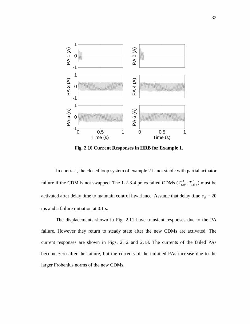
Fig. 2.10 Current Responses in HRB for Example 1.

In contrast, the closed loop system of example 2 is not stable with partial actuator

failure if the CDM is not swapped. The 1-2-3-4 poles failed CDMs ( BA TT 12341234 , ) must be

activated after delay time to maintain control invariance. Assume that delay time dτ = 20

ms and a failure initiation at 0.1 s.

The displacements shown in Fig. 2.11 have transient responses due to the PA

failure. However they return to steady state after the new CDMs are activated. The

current responses are shown in Figs. 2.12 and 2.13. The currents of the failed PAs

become zero after the failure, but the currents of the unfailed PAs increase due to the

larger Frobenius norms of the new CDMs.

33

-0.05

0

0.05

X1 A (m

m)

X1 B

(mm

)

-0.05

0

0.05

X2 A (m

m)

0 0.1 0.2

X2 B

(mm

)

Time (s)

0 0.1 0.2-0.1

0

0.1

X3 A (m

m)

Time (s)

Fig. 2.11 Rotor Displacements in the Radial and Axial Directions for Example 2.

-20 2

PA

1 (A

)

PA

2 (A

)

-20 2

PA

3 (A

)

PA

4 (A

)

-20 2

PA

5 (A

)

PA

6 (A

)

0 0.1 0.2-505

PA

7 (A

)

Time (s)0 0.1 0.2

PA

8 (A

)

Time (s)

Fig. 2.12 Current Responses in HCB for Example 2.

34

0 0.1 0.2-202

PA

1 (A

)

0 0.1 0.2

PA

2 (A

)

-20

2

PA

3 (A

)

PA

4 (A

)

0 0.1 0.2-20

2

PA

5 (A

)

Time (s)0 0.1 0.2

PA

6 (A

)

Time (s)

Fig. 2.13 Current Responses in HRB for Example 2.

Flux densities are shown in Figs. 2.14 and 2.15. The bias flux density in the

radial poles is around 0.7 T for the HRB and 0.72 T for the HCB. The control flux of the

HCB is around 0.03 T (4% of the bias flux) before the failure and 0.1 T (14% of the bias

flux) after the failure. The control flux of the HRB is around 0.015 T (2% of the bias

flux) before the failure and 0.05 T (7% of the bias flux) after the failure. Consequently

the 1-2-3-4 poles failed CDMs satisfy the success criterion for reliability.

35

0.6

0.8

Pol

e 1

(T)

Pol

e 2

(T)

0.6

0.8P

ole

3 (T

)

Pol

e 4

(T)

0.6

0.8

Pol

e 5

(T)

Pol

e 6

(T)

0 0.1 0.2-1

-0.5

0

Pol

e 7

(T)

Time (s)0 0.1 0.2P

ole

8 (T

)Time (s)

Fig. 2.14 Flux Density Responses in HCB for Example 2.

0.6

0.8

Pol

e 1

(T)

Pol

e 2

(T)

0.6

0.8

Pol

e 3

(T)

Pol

e 4

(T)

0 0.1 0.2

0.6

0.8

Pol

e 5

(T)

Time (s)0 0.1 0.2

Pol

e 6

(T)

Time (s)

Fig. 2.15 Flux Density Responses in HRB for Example 2.

36

When contacts between the rotor and the catcher bearings happen during

swapping the CDMs, the rotor may be re-levitated. Figure 2.16 shows the displacements

for a successful re-levitation event with poles 1-2-3-4 failed, dτ =100 ms, µ=0.1,

cC =5,000 N-s/m, and cK =108 N/m.This is highly dependent on whether backward whirl

develops during the contact period. The backward whirl state occurs due to friction at the

contact interface between the shaft and the catcher bearings, which forces the shaft to

whirl (precess) in a direction opposite to the spin direction.

-0.2

0

0.2

X1 A (m

m)

X1 B

(mm

)

-0.2

0

0.2

X2 A (m

m)

0 0.1 0.2 0.3

X2 B (m

m)

Time (s)

0 0.1 0.2 0.3-0.2

0

0.2

X3

(mm

)

Time (s)

Fig. 2.16 Rotor Displacements in the Radial and Axial Directions during Successful Re-levitation.

37

Figure 2.17 shows an example of this state with µ=0.3, cC =105 N-s/m, and

cK =108 N/m. The backward whirl eccentricity is the catcher bearing clearance (typically

0.25 mm) for a rigid rotor and possibly a much larger value for a flexible shaft. The

whirl frequency typically ranges from 0.4-1.0 times the spin frequency. This creates a

potentially large centrifugal force that can damage the catcher bearings or deflect the

shaft into the magnetic bearings. The backward whirl condition is mitigated by proper

design of the flexible damped support, preload, clearance, and friction coefficient for the

catcher bearings. Re-levitation off of the catcher bearings is very difficult once backward

whirl has fully developed.

-0.3 -0.2 -0.1 0 0.1 0.2 0.3

-0.2

-0.1

0

0.1

0.2

0.3

X1A (mm)

X2 A (m

m)

CB ClearanceRotor Orbit

Fig. 2.17 Orbit Plot of the Rotor at CB (A).

38

2.6.5 Reliabilities of 4, 6, and 7 Pole HOMBs

Table 2.4 Summary of Simulation for Reliability Study.

No. of Pole

Failed Bearing

No. of unfailed

Poles

No. of Simulation

SwappingCDM

)( kα

Non-Swapping

CDM )( kα

2 6 4 4 3 4 4 4 Radial 4 1 1 1 2 6 4 4 3 4 4 4

4

Combo 4 1 1 1 2 15 12 0 3 20 20 8 4 15 15 12 5 6 6 6

Radial

6 1 1 1 2 15 12 0 3 20 20 8 4 15 15 12 5 6 6 6

6

Combo

6 1 1 1 2 21 16 0 3 35 33 0 4 35 35 14 5 21 21 21 6 7 7 7

Radial

7 1 1 1 2 21 13 0 3 35 28 2 4 35 35 14 5 21 21 20 6 7 7 7

7

Combo

7 1 1 1

39

The reliability of a magnetic bearing is determined by considering the number of

failed pole states that still meet the success criterion. This is dependent on the delay

time, modeling assumptions, number of poles in the bearing, and the reliability of the

power amplifier/coil units that drive and conduct the bearing currents. The 4 pole and 7

pole configurations require 2 less or 1 more power amplifiers than the 6 pole

configuration, respectively. The radial pole and permanent magnet cross-section areas,

the number of turns of each radial coil, and the coercive force and the length of the

permanent magnets for the 4 and 7 pole bearings are identical to those of the 6 pole

bearing.

Two FTC approaches are utilized for the reliability study. The swapping CDMs

approach is that the radial pole failure simulations are conducted with the combo bearing

operating in a no-pole failed state, and vice versa. Failure occurs at 0.1 seconds into the

simulation and swapping in of the new CDM occurs at a delay time 20 ms later. The

other is the non-swapping approach, which maintains the no-pole failed CDMs. Table

2.4 summarizes the results of these simulations for swapping in the appropriate poles-

failed (new) CDM and for non-swapping CDMs.

By “k-out-of-n” system structure, (2.54), and Table 2.4, Fig. 2.18 shows system

reliability vs. Rp plots for the 4, 6, and 7 pole HRBs by swapping CDMs approach and

for the 2-axis magnetic bearing (without redundant design, i.e. if one of the two PAs

fails, the magnetic bearing fails). The HRB reliability is improved by increasing the

number of radial poles and by the swapping CDMs approach even if Rp is decreasing

according to the lifetime distribution. Similarly, Fig. 2.19 is for the non-swapping CDM

40

approach (maintain the no-poles failed CDMs). The reliabilities are also dependent on

the system control robustness. Increasing the number of poles does not imply higher

system reliability if the CDMs are not swapped. The reliability of the swapping CDMs

approach is better than the non-swapping approach under the same MIMO control law.

Consequently the HCBs have the same trend as HRBs have.

0 0.1 0.2 0.3 0.4 0.5 0.6 0.7 0.8 0.9 10

0.1

0.2

0.3

0.4

0.5

0.6

0.7

0.8

0.9

1

Rp

Sys

tem

Rel

iabi

lity

4 Pole HRB6 Pole HRB7 Pole HRB2 axis MB

Fig. 2.18 System Reliabilities of 4, 6, and 7 Pole Radial Bearings for Swapping CDMs.

41

0 0.1 0.2 0.3 0.4 0.5 0.6 0.7 0.8 0.9 10

0.1

0.2

0.3

0.4

0.5

0.6

0.7

0.8

0.9

1

Rp

Sys

tem

Rel

iabi

lity

4 Pole HRB6 Pole HRB7 Pole HRB 2 axis MB

Fig. 2.19 System Reliabilities of 4, 6, and 7 Pole Radial Bearings for Non-Swapping CDMs.

42

CHAPTER III

FAULT-TOLERANT CIRCULAR SENSOR ARRAYS

Sensor runout is a major disturbance in rotating machinery supported on

magnetic bearing systems. A circular sensor array with weighting gain matrix (WGM) is

presented which can eliminate higher harmonics of runout even with failed sensors. Two

criteria for sensor array failure and runout reduction are defined for evaluating the sensor

array reliability based on uncoupling 1x and 2x sensing and runout reduction. In general,

the reliability and runout reduction increase as the number of sensors increase. The array

reliability and runout reduction that results by updating the WGM after a sensor failure

is shown to be better than without updating. The methodology is demonstrated by a

simulation of an energy storage flywheel system.

Fig. 3.1 Sensor Array with 8 Sensors.

43

3.1 Weighting Gain Matrix

Figure 3.1 illustrates an 8 sensor array with equal angular spacing around the

circumference of the shaft. The shaft can move in either the 1x or 2x directions and

spins at frequency ω . The objectives of the sensor array are to produce voltages

proportional to 1x and 2x , which are free from cross-coupling between the two

directions and from false motions due to shaft runout.

3.1.1 Shaft Centerline Displacement Measurements

The sensor array output is a weighted sum of all sensor output signals in the

array. The objective is to provide a reliable measurement of the shaft centerline radial

position even if some of the sensors fail and with significant levels of runout. This is

accomplished by determining an appropriate linear mapping between sensor and array

outputs via a WGM. Assume that the array has n independent, identical sensors that have

sensor sensitivity, ξ V/m. Then the WGM is the 2-by-n T matrix defined in the relation

⎥⎥⎥

⎦

⎤

⎢⎢⎢

⎣

⎡=⎥

⎦

⎤⎢⎣

⎡=

ns

ss

d

dTF

vv

V M1

2

1 ξ (3.1)

where F is an n-by-n diagonal matrix which indicates the failure configuration of the

array. The entries in matrix F are binary state: Fii=1 (unfailed) or Fii=0 (failed). The

symbol id in (3.1) represents the displacement measurement along the direction of the

ith sensor, and 1sv and 2sv are the array outputs which correspond to the two transverse

displacements ( 1x and 2x ) of the shaft. Each sensor measurement can be expressed in

terms of the shaft displacements

44

Xxx

d

d

nn

ii

n

Θ=⎥⎦

⎤⎢⎣

⎡

⎥⎥⎥

⎦

⎤

⎢⎢⎢

⎣

⎡=

⎥⎥⎥

⎦

⎤

⎢⎢⎢

⎣

⎡

2

11

sincos

sincos

θθ

θθMMM (3.2)

where iθ is the angle between the ith sensor and axis 1x . By combining (3.2) into (3.1),

the array outputs in terms of shaft centerline displacements become

XTFVs Θ= ξ (3.3)

The constraint from (3.3)

ITF =Θ (3.4)

must be satisfied to maintain invariance between shaft motions and the array outputs in

the presence of sensor failures, where I is the 2-by-2 identity matrix. Then there are 4

linear constraint equations on the Tij given as

01)cos(1

1 =−∑=

ii

n

iii FTθ (3.5)

0)sin(1

1 =∑=

ii

n

iii FTθ (3.6)

0)cos(1

2 =∑=

ii

n

iii FTθ (3.7)

01)sin(1

2 =−∑=

ii

n

iii FTθ (3.8)

45

3.1.2 Sensor Runout Effect

The runout sensed by the ith sensor is expressed as the Fourier series expansion

)]sin()sin()cos()[cos(

)]sin()cos([)(

0

22

0

ikikk

kk

kikiki

ktkktkba

ktkbktkatg

θφωθφω

θωθω

−+−+=

−+−=

∑

∑∞

=

∞

= (3.9)

where k is the number of runout harmonics, ka and kb are Fourier coefficients, ω is

the shaft spin frequency, and

)/(tan 1kkk ab−=φ (3.10)

Similar to (3.1) the sensor array outputs due solely to runout are

⎥⎥⎥

⎦

⎤

⎢⎢⎢

⎣

⎡=⎥

⎦

⎤⎢⎣

⎡=

nr

rr

g

gTF

vv

V M1

2

1 ξ (3.11)

Substitution of (3.9) into (3.11) yields

)cos(0

22jkkjk

kkkrj tkbav ψφωγξ −−+=∑

∞

=

j=1, 2 (3.12)

where

2

1

2

1

)sin()cos( ⎟⎠

⎞⎜⎝

⎛+⎟

⎠

⎞⎜⎝

⎛= ∑∑

==

n

iiijii

n

iiijiijk FTkFTk θθγ j=1, 2 (3.13)

))cos(

)sin((tan

1

1

∑

∑

=

=−= n

iiijii

n

iiijii

jk

FTk

FTk

θ

θψ j=1, 2 (3.14)

46

From (3.12), the kth harmonic of runout is eliminated from the array’s jth output if jkγ

is zero. Thus from (3.12) and (3.13) to eliminate one harmonic, the 4 linear constraint

equations

0)cos(1

=∑=

ii

n

ijii FTkθ j=1, 2 (3.15)

0)sin(1

=∑=

ii

n

ijii FTkθ j=1, 2 (3.16)

must be satisfied. Note that for the 1st harmonic (k=1) of runout, (3.15) and (3.16)

become

0)cos(1

1 =∑=

ii

n

iii FTθ (3.17)

0)cos(1

2 =∑=

ii

n

iii FTθ (3.18)

0)sin(1

1 =∑=

ii

n

iii FTθ (3.19)

0)sin(1

2 =∑=

ii

n

iii FTθ (3.20)

Equations (3.17) and (3.20) contradict (3.5) and (3.8) respectively which means the

fundamental harmonic of runout cannot be eliminated by the sensor array, without

destroying the output invariance.

Next consider harmonics 2 to k with nr unfailed sensors. There exists 4k

constraint equations (3.5-3.8, 3.15 and 3.16 for harmonics 2 to k). Arrange these

constraint equations in the matrix forms

47

jj BAX = j=1, 2 (3.21)

where

rnkn

n

n

n

kkkk

A

×⎥⎥⎥⎥⎥⎥

⎦

⎤

⎢⎢⎢⎢⎢⎢

⎣

⎡

=

21

1

1

1

)sin()sin()cos()cos(


θθθθ

θθθθ

L

L

MMM

L

L

(3.22)

[ ]Tjnjj TTX L1= (3.23)

[ ]TB 0011 L= (3.24)

[ ]TB 00102 L= (3.25)

Equation (3.21) is two de-coupling linear systems of equations with nr unknowns

(Xj). The linear systems may be over-determined (2k>nr), determined (2k=nr), or under-

determined (2k<nr). If the linear system is consistent (at least one exact solution), there

is a unique solution with a minimum-norm of Xj. If the linear system is inconsistent (no

exact solution), the norm of the residual vector (AXj-Bj) can is minimized, however the

solution is not unique unless the matrix A has full column rank [30].

A WGM is calculated to satisfy the constraint equations exactly or approximately

for each failure configuration. There exist (2n-1) failure combinations for an array with n

sensors. Let the n sensors be equally spaced

nii /2)1( πθ −= i=1, 2, …, n

48

and refer to the first n harmonics of runout as the fundamental set. Then the second set

(harmonics n+1 to 2n) has the same constraint equations as the fundamental set and so

on. In addition,

1)cos( =inθ (3.26)

0)sin( =inθ (3.27)

)cos(])cos[( ii jjn θθ =− (3.28)

)sin(])sin[( ii jjn θθ −=− (3.29)

The matrix A in (3.22) that considers the fundamental set becomes

rnn

n

n

n

n

n

n

n

n

A

×

⎥⎥⎥⎥⎥⎥⎥⎥⎥⎥⎥⎥⎥⎥⎥

⎦

⎤

⎢⎢⎢⎢⎢⎢⎢⎢⎢⎢⎢⎢⎢⎢⎢

⎣

⎡

−−

−−=

2

1

1

1

1

1

1

1

1

0011


)2sin()2sin()2cos()2cos(

)2sin()2sin()2cos()2cos(


L

L

L

L

L

L

MMM

L

L

L

L

θθθθθθθθ

θθθθθθθθ

(3.30)

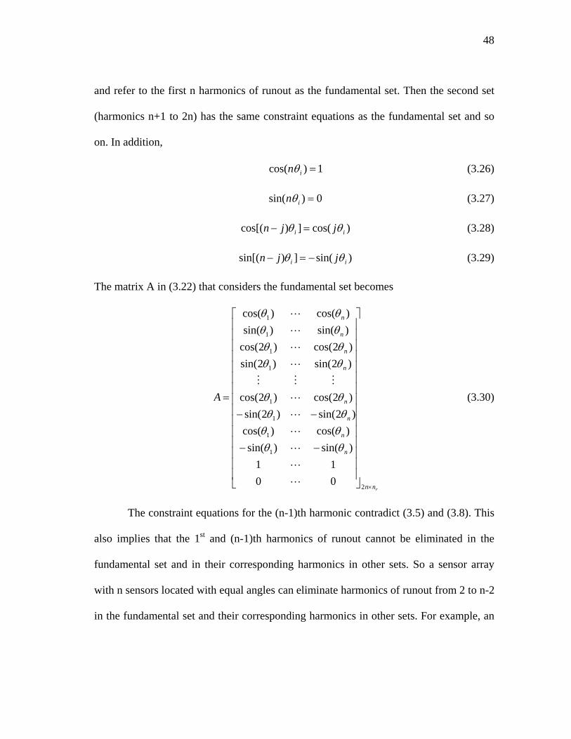
The constraint equations for the (n-1)th harmonic contradict (3.5) and (3.8). This

also implies that the 1st and (n-1)th harmonics of runout cannot be eliminated in the

fundamental set and in their corresponding harmonics in other sets. So a sensor array

with n sensors located with equal angles can eliminate harmonics of runout from 2 to n-2

in the fundamental set and their corresponding harmonics in other sets. For example, an

49

array with 4 sensors can eliminate even harmonics, and an array with 8 sensors can

eliminate harmonics 2 to 6, harmonics 10 to 14 and so on.

3.2 Sensor Array Failure Criterion and Runout Reduction Criterion

Since all of the constraint equations maynot be completely satisfied for the over-

determined systems, some errors will exist in (3.5)-(3.8). Well designed control systems

can tolerate measurement errors depending on the level of robustness. The sensor array

failure criterion is defined based on the controller robustness limits. In practice this is

quantified by considering variation of the sensor array outputs resulting from a myriad of

sensor failure configurations. A measure of the error in array output invariance is

obtained from (3.4) as

ITFE −Θ= (3.31)

The array is considered successful if

ijijE δ≤ , i= 1, 2 j=1,2 (3.32)

where ijδ are constants and selected by considering the robustness of the controller. If

(3.32) is satisfied for a failure combination, then the array is considered unfailed, and the

WGM corresponding to the failure combination is considered successful for the

respective configuration of failed sensors.

The kth component of runout produced the jx array output is zero if jkγ equals

zeros in (3.12) and (3.13). This condition will not always hold if a sensor, or sensors

have failed. Define the user defined tolerance for successful elimination of the kth

50

component of runout as η . Then the array is considered successful for eliminating this

component if

ηγ ≤jk , j=1, 2 (3.33)

If (3.33) is satisfied for a sensor failure configuration, the amplitudes of the kth

harmonics of runout have been reduced at least 100)1( ×−η %, and the WGM is

considered successful for eliminating the kth component of runout.

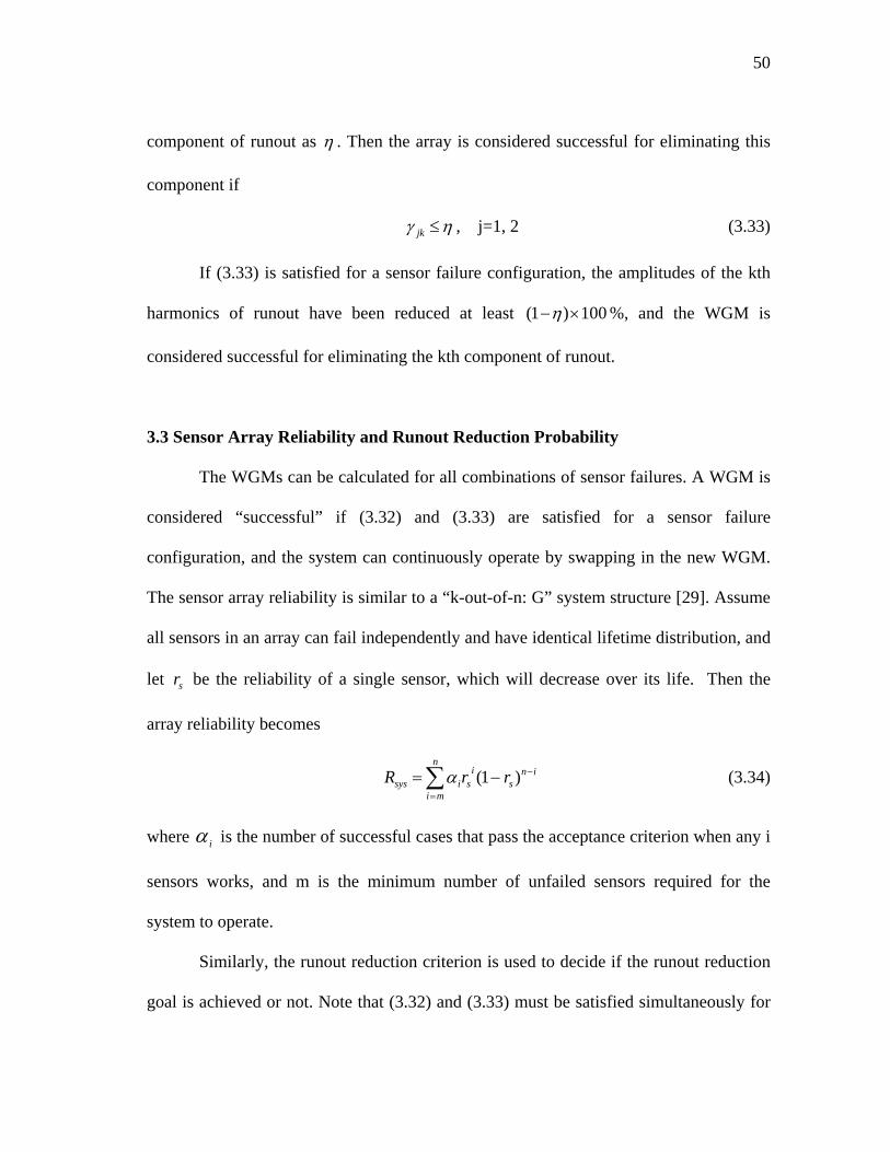
3.3 Sensor Array Reliability and Runout Reduction Probability

The WGMs can be calculated for all combinations of sensor failures. A WGM is

considered “successful” if (3.32) and (3.33) are satisfied for a sensor failure

configuration, and the system can continuously operate by swapping in the new WGM.

The sensor array reliability is similar to a “k-out-of-n: G” system structure [29]. Assume

all sensors in an array can fail independently and have identical lifetime distribution, and

let sr be the reliability of a single sensor, which will decrease over its life. Then the

array reliability becomes

∑=

−−=n

mi

ins

isisys rrR )1(α (3.34)

where iα is the number of successful cases that pass the acceptance criterion when any i

sensors works, and m is the minimum number of unfailed sensors required for the

system to operate.

Similarly, the runout reduction criterion is used to decide if the runout reduction

goal is achieved or not. Note that (3.32) and (3.33) must be satisfied simultaneously for

51

the runout reduction criterion. This is because if the array fails according to the failure

criterion, then the whole system fails. The runout reduction is meaningful only when the

failure criterion is passed. Thus the probability to reach the runout reduction goal for the

kth harmonic of runout becomes

∑=

−−=n

mi

ins

isik rrP )1(β (3.35)

where iβ is the number of successful cases that satisfy both the failure criterion and the

runout reduction criterion.

Since most control systems can tolerate small measurement errors the WGM may

still deliver satisfactory performance if the constraint equations (3.5-3.8, 3.15, 3.16) are

not exactly satisfied. Therefore it is worth while to investigate the array reliability for the

case of retaining the unfailed sensor WGM even after failure of some sensors. The

“swap in approach” (SIA) replaces the existing WGM with the appropriate WGM for the

actual failed sensor configuration. This approach depends on reliable detection of failed

sensors which requires additional hardware. The non-swap-in approach (NSIA) retains

the WGM for the no sensor failed case even if some sensors fail.

3.4 Examples and Simulations

3.4.1 Array Reliability and Runout Reduction Probability

For sake of illustration let ijδ =0.2, η =0.2, ∈sr {0.9, 0.95, 0.99, 0.999}, n=8 and

consider runout harmonics 2 to 6, i.e., 24 constraint equations. Consider three failure

combinations: case 1 for no sensor failure, case 2 for sensor 1 failure, and case 3 for

52

sensor 1 and 2 failure. Table 3.1 shows that the sensor array can completely eliminate

harmonics 2 to 6 for case 1 and case 2 by the SIA. The SIA yields the same degree of

elimination for any one-sensor failure case. Table 3.2 compares the same variables as

Table 3.1 utilizing the NSIA. Note that the runout elimination is imperfect even if just

one sensor fails.

Table 3.1 k1γ and k2γ vs. Harmonics (SIA).

Case 1 Case 2 Case 3 k k1γ k2γ

k1γ k2γ

k1γ k2γ

1 1 1 1 1 0.981 0.885 2 0 0 0 0 0.048 0.116 3 0 0 0 0 0.063 0.152 4 0 0 0 0 0.068 0.165 5 0 0 0 0 0.063 0.152 6 0 0 0 0 0.048 0.116 7 1 1 1 1 0.981 0.885 8 0 0 2 0 1.707 0.707

Table 3.2 k1γ and k2γ vs. Harmonics (NSIA).

Case 1 Case 2 Case 3 k k1γ k2γ

k1γ k2γ

k1γ k2γ

1 1 1 0.75 1 0.637 0.884 2 0 0 0.25 0 0.306 0.177 3 0 0 0.25 0 0.177 0.177 4 0 0 0.25 0 0.073 0.177 5 0 0 0.25 0 0.177 0.177 6 0 0 0.25 0 0.306 0.177 7 1 1 0.75 1 0.637 0.884 8 0 0 0.25 0 0.427 0.177

53

Table 3.3 lists the number of successful cases for SIA and Table 3.4 for NSIA.

For the failure configurations with one or two failed sensors, the SIA has more cases

which satisfy the criterion when considering harmonics 2 to 6. When more than two

sensors fail, no failure configurations can satisfy the criterion by both approaches.

Table 3.3 Number of Successful Cases (SIA).

)( 88 αβ )( 77 αβ )( 66 αβ

n=8 1 8 8 k=1 0 0 0 k=2 1 8 8 k=3 1 8 8 k=4 1 8 8 k=5 1 8 8 k=6 1 8 8 k=7 0 0 0 k=8 1 0 0

All other )( ii αβ are zeros.

Table 3.4 Number of Successful Cases (NSIA).

)( 88 αβ )( 77 αβ )( 66 αβ

n=8 1 4 4 k=1 0 0 0 k=2 1 4 4 k=3 1 4 4 k=4 1 4 4 k=5 1 4 4 k=6 1 4 4 k=7 0 0 0 k=8 1 4 4

All other )( ii αβ are zeros.

54

By (3.34) and (3.35) and Tables 3.3 and 3.4, Tables 3.5 and 3.6 list array

reliability and runout reduction probability vs. sensor reliability. The array reliability

and runout reduction probabilities for harmonics 2 to 6 by SIA are higher than those by

NSIA.

Table 3.5 Sensor Array Reliability and Runout Reduction Probability vs. sr (SIA).

sr =0.900 sr =0.950 sr =0.990 sr =0.9990 Rsys 0.855620 0.957457 0.998063 0.999980 P1 0 0 0 0 P2 0.855620 0.957457 0.998063 0.999980 P3 0.855620 0.957457 0.998063 0.999980 P4 0.855620 0.957457 0.998063 0.999980 P5 0.855620 0.957457 0.998063 0.999980 P6 0.855620 0.957457 0.998063 0.999980 P7 0 0 0 0 P8 0.430467 0.663420 0.922744 0.992027

Table 3.6 Sensor Array Reliability and Runout Reduction Probability vs. sr (NSIA).

sr =0.900 sr =0.950 sr =0.990 sr =0.999 Rsys 0.621786 0.803088 0.960027 0.996000 P1 0 0 0 0 P2 0.621786 0.803088 0.960027 0.996000 P3 0.621786 0.803088 0.960027 0.996000 P4 0.621786 0.803088 0.960027 0.996000 P5 0.621786 0.803088 0.960027 0.996000 P6 0.621786 0.803088 0.960027 0.996000 P7 0 0 0 0 P8 0.621786 0.803088 0.960027 0.996000

55

Tables 3.7 and 3.8 list SIA and NSIA array reliability vs. number of sensors and

sr when harmonics 2 to 6 are considered in each array. Figure 3.2 shows that the SIA

array reliability is better than the NSIA.

Table 3.7 Sensor Array Reliability vs. Number of Sensor and sr (SIA).

sr =0.900 sr =0.950 sr =0.990 sr =0.999 n=8 0.855620 0.957457 0.998063 0.999980 n=9 0.839145 0.951852 0.997780 0.999977

n=10 0.826975 0.947906 0.997589 0.999975 n=11 0.815066 0.943982 0.997398 0.999973 n=12 0.847030 0.957635 0.998214 0.999982 n=13 0.820690 0.948380 0.997742 0.999977 n=14 0.899906 0.974754 0.998998 0.999990 n=15 0.986353 0.998921 0.999998 1.000000 n=16 0.994271 0.999665 1.000000 1.000000

Table 3.8 Sensor Array Reliability vs. Number of Sensor and sr (NSIA).

sr =0.900 sr =0.950 sr =0.990 sr =0.999 n=8 0.621786 0.803088 0.960027 0.996000 n=9 0.645701 0.829276 0.968882 0.996988

n=10 0.736099 0.913862 0.995734 0.999955 n=11 0.736099 0.913862 0.995734 0.999955 n=12 0.728738 0.911577 0.995634 0.999954 n=13 0.724902 0.911502 0.995706 0.999955 n=14 0.737141 0.919963 0.996385 0.999963 n=15 0.730080 0.920301 0.996602 0.999966 n=16 0.741971 0.925877 0.996960 0.999970

56

0 0.1 0.2 0.3 0.4 0.5 0.6 0.7 0.8 0.9 10

0.1

0.2

0.3

0.4

0.5

0.6

0.7

0.8

0.9

1

One Sensor Reliability

Arra

y R

elia

bilit

y

n=8 (SIA)n=16(SIA)n=24(SIA)n=8 (NSIA)n=16(NSIA)n=24(NSIA)

Fig. 3.2 Array Reliability vs. sr .

Fig. 3.3 Control Scheme with Sensor Arrays.

57

3.4.2 System Simulations with Sensor Failures

The flywheel-based magnetic suspension system in CHAPTER II is utilized to

simulate the function of sensor arrays. The system control scheme in Fig. 3.3 uses one

sensor for measuring the axial displacement and two sensor arrays: one for the

axial/radial bearing and the other for the radial bearing. Each sensor in an array is

represented by a 1st older filter with cut-off frequency 5 kHz and sensitivity 7874 V/m.

0 2 4 60

2

4

PA

1 (A

)

0 2 4 60

2

4P

A 2

(A)

0 2 4 60

2

4

PA

3 (A

)

0 2 4 60

2

4

PA

4 (A

)

0 2 4 60

2

4

PA

5 (A

)

Frequency (kHz)0 2 4 6

0

2

4

PA

6 (A

)

Frequency (kHz)

Fig. 3.4 Frequency Spectrum of Currents in HRB for n=2.

Assume that the two sensor arrays have identical sensor failure combinations and

sense identical runout patterns. This results in the same runout harmonics to be reduced

in all 4 outputs of the 2 sensor arrays, and consequently in the power amplifier currents.

58

The first 6 harmonics of runout are considered and have amplitude 0.02 mm, i.e.,

== kk ba 0.02 mm.

Figure 3.4 shows the frequency spectrum of currents in the radial bearing for a

two-sensor (n=2 and sensors are orthogonal) system. All harmonics of runout exist so

the two-sensor system fails to eliminate the runout.

0 2 4 60

2

4

PA

1 (A

)

0 2 4 60

2

4P

A 2

(A)

0 2 4 60

2

4

PA

3 (A

)

0 2 4 60

2

4

PA

4 (A

)

0 2 4 60

2

4

PA

5 (A

)


0

2

4

PA

6 (A

)

Frequency (kHz)

Fig. 3.5 Frequency Spectrum of Currents in HRB for n=4.

Figure 3.5 shows that for a sensor array with 4 sensors, the even harmonics are

eliminated. Figure 3.6 shows that for case 1 (n=8) the higher harmonics are completely

59

eliminated except for the synchronous frequency. The case 2 (n=8) result is identical

with case 1. Figure 3.7 is a zoomed-in range for case 3. The amplitude of the

synchronous frequency in Fig. 3.7 is the same as in Fig. 3.6. The higher harmonics are

not completely eliminated since the constraint equations are not completely satisfied.

0 2 4 60

2

4

PA

1 (A

)

0 2 4 60

2

4

PA

2 (A

)

0 2 4 60

2

4

PA

3 (A

)

0 2 4 60

2

4

PA

4 (A

)

0 2 4 60

2

4

PA

5 (A

)


0

2

4

PA

6 (A

)

Frequency (kHz)

Fig. 3.6 Frequency Spectrum of Currents in HRB for Cases 1 and 2.

60

0 2 4 60

0.1

0.2P

A 1

(A)

0 2 4 60

0.1

0.2

PA

2 (A

)0 2 4 6

0

0.10.2

PA

3 (A

)

0 2 4 60

0.10.2

PA

4 (A

)

0 2 4 60

0.10.2

PA

5 (A

)


0

0.10.2

PA

6 (A

)

Frequency (kHz)

Fig. 3.7 Frequency Spectrum of Currents in HRB for Case 3 (Zoomed-in).

61

CHAPTER IV

ADAPTIVE CONTROL OF HOMOPOLAR MAGNETIC BEARINGS

Fault tolerant control is able to accommodate the system component faults such

as the failures of actuators, sensors, and plants. Normally the operation of fault tolerant

control depends on highly reliable fault detection and identification to detect the faults

by the signal- or model-based approach. In this chapter, two adaptive control schemes

are utilized to compensate for the actuator (power amplifier) failure in a magnetic

suspension system. The gain scheduling adaptive control is combined with the signal-

based fault detection to identify the failure combinations of the power amplifiers. The

other scheme is that the signal-based fault detection is replaced by the model-based fault

detection (estimator). The adaptive law which estimates the jump parameters in a system

is derived by the Lyapunov approach. To reduce the number of persistently exciting

signals, the reduced-order adaptive law is developed. The simulation results of a

magnetic suspension system show that the system can continuously operate when some

of the power amplifiers in a magnetic bearing fail. Thus, the reliability of a magnetic

bearing is improved by the adaptive control schemes.

4.1 Simplified Dynamic Model of a Magnetic Suspension System

A simplified dynamic model which neglects the housing dynamics is shown in

Fig. 4.1. The equations of motion then become

62

Fig. 4.1 Flywheel System with a Magnetic Suspension (Simplified).

( ) ( ) grdrdrcrTCB

rbrTMB

rrrrr FFBFTFTXGXM +++=+ ˆˆˆ&&& (4.1)

which is the same as in (2.36). Arrange these EOMs into state space form

gdrpdcrpcbrpbpprp FFBFBFBXAX ++++= ˆˆˆ& (4.2)

where

[ ]TTr

Trp XXX &= (4.3)

⎥⎦

⎤⎢⎣

⎡−

= −×

××

rrpr GM

IA 1

55

5555

00

(4.4)

⎥⎦

⎤⎢⎣

⎡= −

×TMB

rrpb TM

B)(

01

55 (4.5)

⎥⎦

⎤⎢⎣

⎡= −

×TCB

rrpc TM

B)(

01

55 (4.6)

63

⎥⎦

⎤⎢⎣

⎡= −

×

drrpd BM

B 1450

(4.7)

grrg FMF 1−= (4.8)

The linearized magnetic forces for small angle motions are given as

cvmbrpmbbr VKXKF ˆˆˆ += (4.9)

where the matrices pmbK and vmbK are the position and control voltage stiffness matrices

for the magnetic bearings and the vector cV is the control voltages in the CG coordinate.

The magnetic forces can also be expressed in terms of the bearing coordinate

cMB

rvmbMB

rpmbb VTKXTKF +=ˆ (4.10)

where the control voltage cV is determined by the feedback control. The first term on the

right-hand side of (4.10) is the magnetic forces due to the rotor displacements, which is

not functions of the controller parameters. Substitution of (4.10) in (4.2) yields

gdrpdcrpccpppp FFBFBVBXAX ++++= ˆˆ& (4.11)

where

( ) ⎥⎦

⎤⎢⎣

⎡=⎥

⎦

⎤⎢⎣

⎡−

= −−××

222111

5555 00

pprrMB

rpmb

TMBrr

p AAI

GMTKTMI

A (4.12)

( ) ⎥⎦

⎤⎢⎣

⎡=⎥

⎦

⎤⎢⎣

⎡= −

×

21

55 00

pMB

rvmb

TMBrr

p BTKTMB (4.13)

Notice that the magnetic bearings utilize the permanent magnets to supply the

bias flux and the power amplifiers to supply the control flux. Then the matrix pmbK will

not be influenced by the power amplifier failures, but the matrix vmbK will change

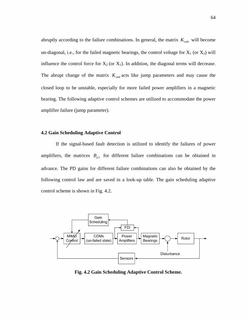
64

abruptly according to the failure combinations. In general, the matrix vmbK will become

un-diagonal, i.e., for the failed magnetic bearings, the control voltage for X1 (or X2) will

influence the control force for X2 (or X1). In addition, the diagonal terms will decrease.

The abrupt change of the matrix vmbK acts like jump parameters and may cause the

closed loop to be unstable, especially for more failed power amplifiers in a magnetic

bearing. The following adaptive control schemes are utilized to accommodate the power

amplifier failure (jump parameter).

4.2 Gain Scheduling Adaptive Control

If the signal-based fault detection is utilized to identify the failures of power

amplifiers, the matrices 2pB for different failure combinations can be obtained in

advance. The PD gains for different failure combinations can also be obtained by the

following control law and are saved in a look-up table. The gain scheduling adaptive

control scheme is shown in Fig. 4.2.

Fig. 4.2 Gain Scheduling Adaptive Control Scheme.

65

Assume that the feedback control law is given as

[ ] rXKKrXKV pfbfbpfbc +−=+−= 21 (4.14)

where the matrix fbK is the feedback gains and the vector r is the reference signals. The

closed loop system matrix becomes

⎥⎦

⎤⎢⎣

⎡−−

=22221221

0

fbppfbpppcl KBAKBA

IA (4.15)

Let the desired closed loop system matrix have the following form

⎥⎦

⎤⎢⎣

⎡=

2221

0

ttt AA

IA (4.16)

where 21tA and 22tA are negative definite, constant matrices or tA is a stable constant

matrix. Then the feedback gains become

)( 21211

21 tppfb AABK −= − (4.17)

)( 22221

22 tppfb AABK −= − (4.18)

By (4.17) and (4.18), the feedback gains for different failure combinations can be

calculated in advance.

4.3 Adaptive Pole Placement Control

The adaptive pole placement control (APPC) scheme is shown in Fig. 4.3. For

APPC, the first step is to estimate the plant parameters. If the matrices pA and pB are

unknown, the adaptive law in [31] can be utilized. The parameter convergence is

guaranteed by persistent excitation.

66

Fig. 4.3 Adaptive Pole Placement Control Scheme.

If some of the parameters are known, the order of the adaptive law and the

number of persistently exciting signals can be reduced. Assume that the matrix pA is

known but the matrix pB is unknown, which corresponds to the failures of power

amplifiers. In the following, the reduced-order adaptive law is developed by the SPR-

Lyapunov approach. Let

[ ] [ ]TTTTTTp XXXXX 21== & (4.19)

By neglecting the disturbances, then (4.11) becomes

21 XX =& (4.20)

cppp VBXAXAX 22221212 ++=& (4.21)

Assume that all states are measurable and mA is a stable constant matrix. By adding and

subtracting 2XAm on (4.21) and using Laplace transform, we obtain

cpmmppm VBAsIXAAXAAsIXZ 21

2221211

2 )(])([)( −− −=−+−−= (4.22)

67

Note that the matrix 2pB is the only unknown term in (4.22). By the series-parallel (SP)

model, we generate

cpm VBAsIZ 21 ˆ)(ˆ −−= (4.23)

where Z and 2ˆ

pB are the estimates of Z and 2pB , respectively. Then define the

following auxiliary signals

ZZe ˆ−= (4.24)

222ˆ~

ppp BBB −= (4.25)

From (4.22) to (4.25), the error equation becomes

cpm VBeAe 2~−=& (4.26)

The error equation is only for analysis, not for implementation since the matrix 2~

pB is

not known exactly. Choose the Lyapunov function

)~~()~,( 21

22 pT

pmT

p BBtrePeBeV −Γ+= (4.27)

where Γ and mP are symmetric, positive definite, constant matrices. In addition, mP

satisfies the Lyapunov equation

mmmmT

m QAPPA −=+ (4.28)

for some 0>= mT

m QQ . Choose the adaptive law

Tcmpp eVPBB Γ== 22

ˆ~ && (4.29)

Then the derivative of the Lyapunov function becomes

0)( 2min ≤−≤−= eQeQeV mm

T λ& (4.30)

68

where )(min mQλ is the smallest eigenvalue of mQ .

The Lyapunov function V is positive definite and decrescent; the derivative of V

is semi-definite. From the Lyapunov stability theorem, the equilibrium state

( )0~,0 1 == pBe of (4.26) and (4.29) is locally uniformly stable. Assume that pX and cV

are bounded. Then the adaptive law guarantees that 0)( →te and 0ˆ2 →pB& as ∞→t , but

it does not imply parameter convergence. If the plant input signals are persistently

exciting, then the parameters will converge to the true values.

The second step of APPC is the controller design, which maps the estimated

plant parameters to the controller parameters. The controller design in gain scheduling

can be utilized. Thus, the estimated gains become

)(ˆˆ2121

121 tppfb AABK −= − (4.31)

)(ˆˆ2222

122 tppfb AABK −= − (4.32)

4.4 Simulations by Adaptive Control

An example flywheel module illustrates the operation of active FTC. Each

magnetic bearing has 6 radial poles. The position stiffness matrix of two magnetic

bearings is given as

( ) 6103889.13889.13754.10043.10043.1 ×= diagK pmb N/m

Notice that the values are not influenced by the failure of power amplifiers. The control

voltage stiffness matrix for no PA failed state is given as

69

( )4822.144822.141317.131317.131316.130 diagKvmb = N/V

Consider the case that two magnetic bearings have the same failure combinations

and power amplifiers 1 to 3 fail consecutively. The control voltage stiffness matrices for

failed states are given as follows

⎥⎥⎥⎥⎥⎥

⎦

⎤

⎢⎢⎢⎢⎢⎢

⎣

⎡

−−

−−

=

2753.130903.20000903.28617.10000001317.13000000374.128954.10008954.18487.9

1vmbK N/V

⎥⎥⎥⎥⎥⎥

⎦

⎤

⎢⎢⎢⎢⎢⎢

⎣

⎡

−−

−−

=

4479.80903.20000903.28617.10000001317.13000006601.78954.10008954.18487.9

12vmbK N/V

( )2411.72411.71317.135658.65658.6123 diagKvmb = N/V

According to (4.13), the matrices 2pB corresponding to different vmbK become

⎥⎥⎥⎥⎥⎥

⎦

⎤

⎢⎢⎢⎢⎢⎢

⎣

⎡

−

−

=

4430.0000009737.1003419.0009315.00030.00003419.09737.1000030.0009315.0

02pB

⎥⎥⎥⎥⎥⎥

⎦

⎤

⎢⎢⎢⎢⎢⎢

⎣

⎡

−−−

−−−

=

4430.0000004802.10493.02849.02564.000004.08539.00028.01345.002849.03134.08092.10494.000023.01345.00004.06986.0

12pB

70

⎥⎥⎥⎥⎥⎥

⎦

⎤

⎢⎢⎢⎢⎢⎢

⎣

⎡

−−−

−−−

=

4430.0000004802.10493.02849.02564.000004.05434.00018.01345.002849.01994.01513.10493.000023.01345.00004.06986.0

122pB

⎥⎥⎥⎥⎥⎥

⎦

⎤

⎢⎢⎢⎢⎢⎢

⎣

⎡

−

−

=

4430.0000009868.0001710.0004658.00015.00001710.09868.0000015.0004658.0

1232pB

The disturbances are given by

[ ]Trd ttttemF )sin()cos()sin()cos(ˆ 2 ψωψωωωω ++=

The desired closed loop matrices are given as

⎥⎥⎥⎥⎥⎥

⎦

⎤

⎢⎢⎢⎢⎢⎢

⎣

⎡

−−−−−−−−−−

⋅=

1520.2000009614.206622.48864.000071.03931.10078.0006622.48865.09614.2000078.000071.03931.1

10521tA

⎥⎥⎥⎥⎥⎥

⎦

⎤

⎢⎢⎢⎢⎢⎢

⎣

⎡

−−

−−−−−

−

⋅=

5232.0000002331.004324.20404.000004.01100.00004.0004324.20404.02331.0000004.000004.01100.0

10322tA

Then the eigenvalues of the closed loop system become

71

⎥⎥⎥⎥⎥⎥⎥⎥⎥⎥⎥⎥⎥⎥

⎦

⎤

⎢⎢⎢⎢⎢⎢⎢⎢⎢⎢⎢⎢⎢⎢

⎣

⎡

=

i383.1 -261.60-i383.1 + 261.60-

i369.07 - 54.931-i369.07 + 54.931-i369.3 - 54.918-i369.3 + 54.918-

i112.64 - 185.47-112.64 i+ 185.47-

i2545.3 - 47.810-i2545.3 +0 47.81-

Eig

4.4.1 Simulations by Gain Scheduling

When the power amplifier failures happen, a period of time (delay time) is

needed to isolate the fault and to swap the feedback gains from the look-up tables.

Assume that the initial failures of the power amplifiers are at 1 s, 2 s, and 3 s

consecutively and the delay time is 100 ms. The control law is combined with the

integrators. The rotor displacements and control magnetic forces by the gain scheduling

approach are shown in Figs. 4.4 and 4.5. The rotor is continuously suspended without

contacts through the entire simulation. The axial displacement due to the gravity

becomes zero by using the integrator. During each delay time, the magnetic forces are

reduced since the smaller matrix norms of the control voltage stiffness matrices for the

failed states. The gain values for the failed states can make the closed loop responses

invariant.

72

0 1 2 3 4-0.05

0

0.05

X1 A (m

m)

0 1 2 3 4-0.05

0

0.05

X2 A (m

m)

0 1 2 3 4-0.06

-0.04-0.02

0

X3 A (m

m)

Time (s)

0 1 2 3 4-0.05

0

0.05

X1 B

(mm

)

0 1 2 3 4-0.05

0

0.05

X2 B

(mm

)

Time (s)

Fig. 4.4 Rotor Displacements by Gain Scheduling.

0 1 2 3 4-100

0

100

Fx1 A (N

)

0 1 2 3 4-100

0

100

Fx2 A (N

)

0 1 2 3 40

200400600

Fx3 A (N

)

0 1 2 3 4-100

0

100

Fx1 B

(N)

0 1 2 3 4-100

0

100

Fx2 B

(N)

Fig. 4.5 Control Magnetic Forces by Gain Scheduling.

73

4.4.2 Simulations by APPC

To identify the system on-line, the inputs and outputs of the plant cannot be zero.

The following reference signals and design parameter are utilized for the simulations

⎥⎥⎥⎥⎥⎥

⎦

⎤

⎢⎢⎢⎢⎢⎢

⎣

⎡

+++++

⋅=

)65sin()60sin()55sin()50sin()45sin()40sin()35sin()30sin()25sin()20sin(

2

tttttttttt

r

5510 ×⋅−= IAm , 55100 ×⋅= IQm , and 55100 ×⋅=Γ I .

Three examples are utilized to demonstrate the fault tolerant operation by APPC.

The first example considers the case without disturbances (gravity and mass unbalance).

Only consider the failures (open circuit) of the power amplifiers, and assume that the

initial failures are at 20 s, 40 s, and 60 s, respectively. The rotor displacements and

control magnetic forces are shown in Figs. 4.6 and 4.7, and the estimated parameters are

shown in Figs. 4.8-4.12. The displacements and control magnetic forces are due to the

reference signals which are necessary to identify the system parameters. The simulations

show that the estimated parameters converge to the true values of each failed state by

persistently exciting signals.

74

0 20 40 60 80-0.05

0

0.05

X1 A (m

m)

0 20 40 60 80-0.05

0

0.05

X2 A (m

m)

0 20 40 60 80-0.01

0

0.01

X3 A (m

m)

Time (s)

0 20 40 60 80-0.05

0

0.05

X1 B

(mm

)

0 20 40 60 80-0.05

0

0.05

X2 B

(mm

)

Time (s)

Fig. 4.6 Rotor Displacements Example 1 by APPC.

0 20 40 60 80-50

0

50

Fx1 A (N

t)

0 20 40 60 80-50

0

50

Fx2 A (N

t)

0 20 40 60 80-20

0

20

Fx3 A (N

t)

Time (s)

0 20 40 60 80-50

0

50

Fx1 B

(Nt)

0 20 40 60 80-50

0

50

Fx2 B

(Nt)

Time (s)

Fig. 4.7 Control Magnetic Forces Example 1 by APPC.

75

0.5

1

Bp2

(1,1

)

-0.40

0.4B

p2(2

,1)

-0.4-0.2

0

Bp2

(3,1

)

-0.40

0.4

Bp2

(4,1

)

0 10 20 30 40 50 60 70 80-0.1

00.1

Bp2

(5,1

)

Time (s)

Fig. 4.8 Estimated Parameters (Column 1) Example 1 by APPC.

-0.20

0.2

Bp2

(1,2

)

11.5

2

Bp2

(2,2

)

-0.40

0.4

Bp2

(3,2

)

-0.40

0.6

Bp2

(4,2

)

0 10 20 30 40 50 60 70 80-0.1

00.1

Bp2

(5,2

)

Time (s)


76

-0.4-0.2

00.2

Bp2

(1,3

)

00.20.4

Bp2

(2,3

)

0.5

1

Bp2

(3,3

)

-0.20

0.2

Bp2

(4,3

)

0 10 20 30 40 50 60 70 80-0.1

00.1

Bp2

(5,3

)

Time (s)


-0.20

0.2

Bp2

(1,4

)

-0.40

0.6

Bp2

(2,4

)

-0.20

0.2

Bp2

(3,4

)

11.5

2

Bp2

(4,4

)

0 10 20 30 40 50 60 70 80-0.1

00.1

Bp2

(5,4

)

Time (s)


77

-0.20

0.2

Bp2

(1,5

)

-0.20

0.2B

p2(2

,5)

-0.20

0.2

Bp2

(3,5

)

-0.20

0.2

Bp2

(4,5

)

0 10 20 30 40 50 60 70 800.20.4

Bp2

(5,5

)

Time (s)


The values of CDMs include the power amplifier gains which may decrease over

the time. In the above simulations, the power amplifier gains are fixed and have the

values of 1 A/V. One advantage by APPC over the gain scheduling control is that the

power amplifier gains may decrease over the time and may not be measured. Example 2

considers the case that power amplifiers fail consecutively and the power amplifier gains

linearly decrease to 0.6 A/V during the entire simulation. All of the design parameters

are the same as in Example 1. The rotor displacements and control magnetic forces are

shown in Figs. 4.13 and 4.14. When compared with Example 1, the displacements

decrease over the time. The estimated parameters are shown in Figs. 4.15-4.19. The

estimated parameters follow the variations (jump and linear decreasing).

78

0 20 40 60 80-0.05

0

0.05

X1 A (m

m)

0 20 40 60 80-0.05

0

0.05

X2 A (m

m)

0 20 40 60 80-0.01

0

0.01

X3 A (m

m)

Time (s)

0 20 40 60 80-0.05

0

0.05

X1 B

(mm

)

0 20 40 60 80-0.05

0

0.05

X2 B

(mm

)

Time (s)


0 20 40 60 80-50

0

50

Fx1 A (N

t)

0 20 40 60 80-50

0

50

Fx2 A (N

t)

0 20 40 60 80-20

0

20

Fx3 A (N

t)

Time (s)

0 20 40 60 80-50

0

50

Fx1 B

(Nt)

0 20 40 60 80-50

0

50

Fx2 B

(Nt)

Time (s)


79

0.51

Bp2

(1,1

)

-0.40

0.4B

p2(2

,1)

-0.4-0.2

0

Bp2

(3,1

)

-0.40

0.4

Bp2

(4,1

)

0 10 20 30 40 50 60 70 80-0.1

00.1

Bp2

(5,1

)

Time (s)


-0.20

0.2

Bp2

(1,2

)

1

2

Bp2

(2,2

)

-0.40

0.4

Bp2

(3,2

)

-0.40 0.6

Bp2

(4,2

)

0 10 20 30 40 50 60 70 80-0.1

00.1

Bp2

(5,2

)

Time (s)


80

-0.4-0.2

00.2

Bp2

(1,3

)

00.20.4

Bp2

(2,3

)

0.5

1

Bp2

(3,3

)

-0.20

0.2

Bp2

(4,3

)

0 10 20 30 40 50 60 70 80-0.1

00.1

Bp2

(5,3

)

Time (s)


-0.20

0.2

Bp2

(1,4

)

-0.40

0.6

Bp2

(2,4

)

-0.20

0.2

Bp2

(3,4

)

1

2

Bp2

(4,4

)

0 10 20 30 40 50 60 70 80-0.1

00.1

Bp2

(5,4

)

Time (s)


81

-0.20

0.2

Bp2

(1,5

)

-0.20

0.2B

p2(2

,5)

-0.20

0.2

Bp2

(3,5

)

-0.20

0.2

Bp2

(4,5

)

0 10 20 30 40 50 60 70 800.20.4

Bp2

(5,5

)

Time (s)


Example 3 considers the case with disturbances (mass unbalance and gravity).

Only power amplifier failures are considered. According to [32], some filters are utilized

to remove the low-frequency and known sinusoidal disturbances before the plant inputs

and outputs are sent to the estimator. In the following simulations, the high pass and

notch filters are utilized to remove the gravity in the axial direction and the mass

unbalances in the radial directions, respectively. The following design parameters are

utilized for the simulations. 5510 ×⋅−= IAm , 5510 ×⋅= IQm , and

)1.01111(diag=Γ

82

The frequencies of the reference signals are the same as before, but their amplitudes are

increased to 5 (V) to help identify the parameters. In addition, assume that the initial

failures of the power amplifiers are at 200 s, 400 s, and 600 s, respectively.

The displacements and control magnetic forces are shown in Figs. 20 and 21.

The responses are due to the disturbances and reference signals, and their amplitudes are

much large when compared with the gain scheduling approach. The estimated

parameters are shown in Figs. 22-26. Due to the small adaptive gains, the parameters

slowly converge to the true values or the values with steady state errors.

0 200 400 600 800-0.1

0

0.1

X1 A (m

m)

0 200 400 600 800-0.1

0

0.1

X2 A (m

m)

0 200 400 600 800-0.06

-0.04-0.02

0

X3 A (m

m)

Time (s)

0 200 400 600 800-0.1

0

0.1

X1 B

(mm

)

0 200 400 600 800-0.1

0

0.1

X2 B

(mm

)

Time (s)


83

0 200 400 600 800-200

0

200

Fx1 A (N

t)

0 200 400 600 800-200

0

200

Fx2 A (N

t)

0 200 400 600 8000

200

400

Fx3 A (N

t)

Time (s)

0 200 400 600 800-200

0

200

Fx1 B

(Nt)

0 200 400 600 800-200

0

200

Fx2 B

(Nt)

Time (s)


0.5

1

Bp2

(1,1

)

-0.2-0.1

00.1

Bp2

(2,1

)

-0.2-0.1

00.1

Bp2

(3,1

)

-0.4-0.2

0

Bp2

(4,1

)

0 100 200 300 400 500 600 700 800-0.1

00.1

Bp2

(5,1

)

Time (s)


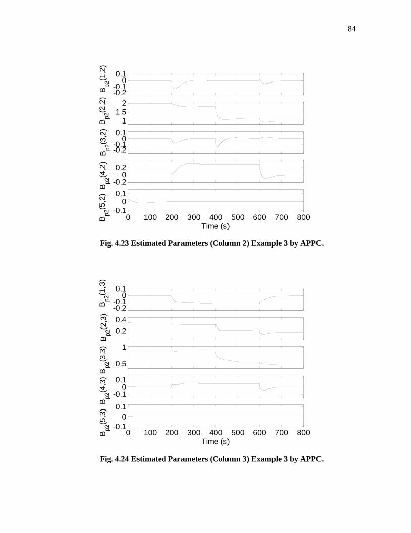
84

-0.2-0.1

00.1

Bp2

(1,2

)

11.5

2B

p2(2

,2)

-0.2-0.1

00.1

Bp2

(3,2

)

-0.20

0.2

Bp2

(4,2

)

0 100 200 300 400 500 600 700 800-0.1

00.1

Bp2

(5,2

)

Time (s)


-0.2-0.1

00.1

Bp2

(1,3

)

0.20.4

Bp2

(2,3

)

0.5

1

Bp2

(3,3

)

-0.10

0.1

Bp2

(4,3

)

0 100 200 300 400 500 600 700 800-0.1

00.1

Bp2

(5,3

)

Time (s)


85

-0.10

0.10.2

Bp2

(1,4

)

00.20.40.6

Bp2

(2,4

)

-0.2-0.1

00.1

Bp2

(3,4

)

11.5

2

Bp2

(4,4

)

0 100 200 300 400 500 600 700 800-0.1

00.1

Bp2

(5,4

)

Time (s)


-0.10

0.1

Bp2

(1,5

)

-0.10

0.1

Bp2

(2,5

)

-0.10

0.1

Bp2

(3,5

)

-0.10

0.1

Bp2

(4,5

)

0 100 200 300 400 500 600 700 8000.30.40.5

Bp2

(5,5

)

Time (s)


86

CHAPTER V

CONCLUSION AND FUTURE RESEARCH

5.1 Conclusion

This dissertation presents the fault tolerant control of homopolar magnetic

bearings and sensor arrays. Successful fault tolerant control has been demonstrated by

two approaches. One approach is to adjust system parameters by swapping current

distribution matrices for magnetic bearings and weighting gain matrices for sensor

arrays, but maintain the MIMO-based control law invariant before and after the faults.

The other is to adjust the feedback gains on-line or off-line, but the current distribution

matrices are invariant before and after the faults. Both approaches can compensate for

the failures (open circuit) of power amplifiers (or coils) and sensors. The simulations

show some interesting results and trends which are summarized as follows.

5.1.1 Fault Tolerant of Homopolar Magnetic Bearings

Current distribution matrices are evaluated based on the set of poles (power

amplifier plus coil) that have failed and the requirements for uncoupled force/voltage

control, linearity, and specified force/voltage gains to be unaffected by the failure. The

first advantage of homopolar magnetic bearings over heteropolar magnetic bearings is

the automatic invariance of the position stiffness before and after pole failure, and the

second advantage is the high efficiency since the bias flux of HOMB is supplied by

permanent magnets.

87

Among 4, 6, and 7 pole homopolar magnetic bearings, successful levitation with

2 unfailed radial poles is demonstrated, and the bearing reliability is increased as the

number of poles increases.

5.1.2 Fault Tolerant of Circular Sensor Arrays

Weighting gain matrices are evaluated based on the set of sensors that have failed

and the requirements for uncoupling 1x and 2x sensing, runout reduction, and

voltage/displacement gains to be unaffected by the failure. The simulations and analysis

presented have confirmed the ability of sensor arrays to eliminate sensor runout. It has

been shown that the more sensors the array has, the more harmonics of runout the array

can eliminate or reduce. Complete runout elimination can be maintained by the SIA if

some sensors fail, but not by the NSIA. Judging from the reliability and runout reduction

probability, SIA is better than NSIA, but of course requires additional hardware for

faulted sensor detection.

Since sensor arrays use more sensors that have failure probability, the array

reliability and runout reduction, which depend on one single sensor reliability, have to be

considered. Two criteria are defined to evaluate the sensor array reliability and runout

reduction probability. A more precise way to decide the array reliability is to do system

simulations in all failure combinations. A sensor array with n sensors has (2n-1) failure

combinations. When n is large, the simulations for all failure combinations are time

consuming and impractical.

It is a trade-off to decide how many sensors in an array and how many harmonics

of runout are considered. If the number of runout harmonics is decided, in general the

88

more sensors the array has, the higher system reliability and runout reduction probability

the array can reach when rs is higher. In addition, the runout reduction performance is

not guaranteed for those harmonics of runout which are not considered in the constraint

equations.

5.1.3 Adaptive Fault Tolerant Control

The simulation results have demonstrated the fault tolerance of power amplifier

failures by two adaptive control schemes. The gain scheduling adaptive control is robust

to the disturbances (gravity and mass unbalance), but the information for failure

configurations is required in advance to build up the feedback gains in the look-up table.

The adaptive law for the linear time invariant plant is utilized to accommodate

the parameter jump. The persistently exciting signals are required to make the jump

parameters converge to the true values of each failed state. However persistent excitation

contradicts the objectives of the regulators and cannot, in general, be avoided.

The amplitudes and frequencies of the reference signals will influence the rate of

parameter convergence. Generally speaking, the larger amplitudes the reference signals

have, the faster the parameters can converge to the true values. Similarly, high adaptive

gains ( mQ and Γ ) can make the parameters converge fast as well, but may make the

closed loop unstable when disturbances are considered.

5.2 Future Research

The adaptive law in Section 4.3 is not robust with respect to the bounded,

unknown disturbances. In addition, the states of controller, actuators, and sensors are

89

neglected in Section 4.3. The adaptive law may excite the un-modeled dynamics. Future

research may develop the robust adaptive pole placement control scheme, which is

robust with respect to bounded, unknown disturbances and un-modeled dynamics.

In Chapter III, the non-swapping-in WGMs approach also makes the

voltage/displacement gains jump. Future research may utilize the adaptive control

scheme to accommodate the sensor failures.

90

REFERENCES

[1] Iwaki, S., 1990, “The Optimal Location of Electromagnets in Multiple Degree of

Freedom Magnetically Suspended Actuators,” ASME J. Dynamic Systems,

Measurement, and Control, 112(4), pp. 690-695.

[2] Meeker, D. C., 1996, “Optimal Solution to the Inverse Problem in Quadratic

Magnetic Actuators,” Ph.D. dissertation, Univ. of Virginia, Charlottesville, VA.

[3] Maslen, E. H., and Meeker, D. C., 1995, “Fault Tolerance of Magnetic Bearings by

Generalized Bias Current Linearization,” IEEE Trans. Magnetics., 31(3), pp. 2304-

2314.

[4] Maslen, E. H., Sortore, C. K., and Gillies, G. T., 1999, “Fault Tolerant Magnetic

Bearings,” ASME J. Engineering for Gas Turbines and Power, 121(3), pp. 504-508.

[5] Na, UJ, and Palazzolo, A., 2000, “Optimized Realization of Fault-Tolerant

Heteropolar Magnetic Bearings,” ASME J. Vibration and Acoustics, 122(3), pp.

209-221.

[6] Na, UJ, Palazzolo, A., and Provenza, A., 2002, “Test and Theory Correlation Study

for a Flexible Rotor on Fault-Tolerant Magnetic Bearings,” ASME J. Vibration and

Acoustics, 124(3), pp. 359-366.

[7] Na, UJ, and Palazzolo, A., 2000, “Fault Tolerance of Magnetic Bearings with

Material Path Reluctances and Fringing Factors,” IEEE Trans. Magnetics, 36(6),

pp. 3939-3946.

[8] Maslen, E. H., Allaire, P. E., Noh, M. D., and Sortore, C. K., 1996, “Magnetic

Bearing Design for Reduced Power Consumption,” ASME J. Tribology, 118(4),

pp. 839-846.

[9] Batty, R., 1988, “Notch Filter Control of Magnetic Bearings to Improve Rotor

Synchronous Response,” MS thesis, Massachusetts Institute of Technology,

Cambridge, MA.

[10] Knospe, C. R., 1991, “Stability and Performance of Notch Filters for Unbalance

Response,” Proceedings of the International Symposium on Magnetic Suspension

Technology, Hampton, VA., p. 181.

91

[11] Bleuler, H., Gahler, C., Herzog, R., Larsonneur, R., Mizuno, T., Siewart, R., and

Woo, S.-J, 1994, “Application of Digital Signal Processors for Industrial Magnetic

Bearings,” IEEE Trans. on Control Systems Technology, 2(4), pp. 280-289.

[12] Herzog, R., Buhler, P., Gahler, C., and Larsonneur, R., 1996, “Unbalance

Compensation Using Generalized Notch Filters in Multivariable Feedback of

Magnetic Bearings,” IEEE Trans. on Control Systems Technology, 4(5), pp. 580-

586.

[13] Na, H.–S., and Park, Y., 1997, “An adaptive Feedforward Controller for Rejection

of Periodic Disturbances,” J. Sound and Vibration, 201(4), pp. 427-435.

[14] Knospe, C. R., Tamer S. M., and Fedigan, S. J., 1997, “Synthesis of Robust Gain

Matrices for Adaptive Rotor Vibration Control,” ASME J. Dynamic Systems


[15] Knospe, C. R., and Tamer S. M., 1997, “Experiments in Robust Control of Rotor

Unbalance Response Using Magnetic Bearings,” Mechatronics, 7(3), pp. 217-229.

[16] Knospe, C. R., Tamer S. M., and Fedigan, S. J., 1997, “Robustness of Adaptive

Rotor Vibration Control to Structured Uncertainty,” ASME J. Dynamic Systems


[17] Betschon, F., and Knospe, C. R., 2001, “Reducing Magnetic Bearing Currents via

Gain Scheduled Adaptive Control,” IEEE/ASME Trans. on Mechatronics, 6(4),

pp.437-443.

[18] Kim, C.-S., and Lee, C.-W., 1997, “In Situ Runout Identification in Active

Magnetic Bearing System by Extended Influence Coefficient Method,”

IEEE/ASME Trans. on Mechatronics, 2(1), pp. 51-57.

[19] Setiawan, J. D., Mukherjee, R., and Maslen, E. H., 2001, “Adaptive Compensation

of Sensor Runout for Magnetic Bearings with Uncertain Parameters: Theory and

Experiments,” ASME J. Dynamic Systems, Measurement, and Control, 123(2), pp.

211-218.

[20] Setiawan, J. D., Mukherjee, R., and Maslen, E. H., 2002, “Synchronous Sensor

Runout and Unbalance Compensation in Active Magnetic Bearings Using Bias

92

Current Excitation,” ASME J. Dynamic Systems, Measurement, and Control,

124(1), pp. 211-218.

[21] Tao, G., Joshi, S. M., and Ma, X., 2001, “Adaptive State Feedback and Tracking

Control of Systems with Actuator Failures,” IEEE Trans. on Automatic Control,

46(1), pp. 78-95.

[22] Tao, G., Chen, S., and Joshi, S. M., 2002, “An Adaptive Actuator Failure

Compensation Controller Using Output Feedback,” IEEE Trans. on Automatic

Control, 47(3), pp. 506-511.

[23] Tao, G., Chen, S., and Joshi, S. M., 2002, “An Adaptive Control Scheme for

Systems with unknown Actuator Failures,” Automatica, 38(6), pp. 1027-1034.

[24] Skogestad, S. and Postlethwaite, I., 1996, Multivariable Feedback Control, John

Wiley & Sons, New York, p. 519, Appendix A.

[25] Sun, G., Palazzolo, A., and Kaushik, N., 2003, “An Efficient Algorithm for Blade

Loss Simulations Using a High Fidelity Ball Bearing and Damper Model,” ASME

Design Engineering Technical Conferences and Computers and Information in

Engineering Conference, Chicago, IL, pp. 1011-1020.

[26] Okada, Y., Nagai, B. and Shimane, T., 1992, “Cross Feedback Stabilization of the

Digitally Controlled Magnetic Bearing,” ASME J. Vibration and Acoustics, 114(1),

pp. 54-59.

[27] Ahrens, M., Traxler, A., Von Burg, P., and Schweitzer, G., 1994, “Design of a

Magnetically Suspended Flywheel Energy Storage Device,” Fourth International

Symposium on Magnetic Bearings, ETH Zurich, Switzerland, pp. 553-558.

[28] Ahrens, M., Kucera, L., and Larsonneur, R., 1996, “Performance of a Magnetically

Suspended Flywheel Energy Storage Device,” IEEE Trans. on Control System

Technology, 4(5), pp. 494-502.

[29] Kuo, W., and Zuo, M., 2003, Optimal Reliability Modeling, John Wiley & Sons,

Hoboken, p. 231, Chap. 7.

[30] Ben-Israel, A., and Greville, T., 2003, Generalized Inverses: Theory and

Applications, Springer-Verlag, New York, p. 105.

93

[31] Ioannou, P. A., and Sun, J., 1995, Robust Adaptive Control, Prentice Hall PTR,

River, NJ, pp. 325-327.

[32] Astrom, K. J., and Wittenmark, B., 1995, Adaptive Control, Addison-Wesley, New

York, pp. 494-495.

94

VITA

Ming-Hsiu Li was born on September 16, 1970, in Taichung County, Taiwan. He

is the first child among four in the family of Shan-Tsao Li. He received his Bachelor of

Science degree in agricultural machinery engineering from National Chung Hsing

University, Taiwan, in June of 1994 and Master of Science degree in aeronautics and

astronautics engineering from National Cheng Kung University, Taiwan, in June of

1996. After a two-year military service in the army and one-and-a-half years as a

mechanical engineer in Phoenixtec Power Co., he enrolled in the Ph.D. program in

mechanical engineering of Texas A&M University in August of 2000. After passing the

qualifying exam and finishing some course work, he has worked with Dr. Palazzolo in

the Vibration Control and Electromechanics Lab (VCEL) since April of 2002. Most of

his research is focused on the fault tolerant control of magnetic bearings.

Ming-Hsiu may be reached at the following address:

6, Ln. 428, Chung-Cheng N. Rd,

Sanchung, Taipei County, 241

Taiwan

fault tolerant control of homopolar...

Documents