fault tolerant control of octorotor using sliding mode ... · 3 sliding mode control synthesis 3.1...

Fault Tolerant Control of Octorotor UsingSliding Mode Control Allocation

Halim Alwi and Christopher Edwards

Abstract This paper presents a fault tolerant control scheme using sliding modecontrol allocation for an octorotor UAV. Compared to the existing literature onquadrotor or octorotor UAVs, the scheme in this paper takes full advantage of theredundant rotors to handle more than one rotor failure. A sliding mode approachis used as the core baseline controller, which is robust against uncertainty in theinput channels – including faults to any of the rotors. Even when total failures oc-cur, no reconfiguration is required to the baseline controller, and the control signalsare simply re-allocated to the remaining healthy rotors using control allocation, tomaintain nominal fault-free performance. To highlight the efficacy of the scheme,various types of rotor fault/failure scenarios have been tested on a nonlinear model.The results show no visible change in performance when compared to the fault-freecase.

1 Introduction

There has been much research interest focussed on UAVs in recent years (see for ex-ample [6, 15, 5, 19]). The quadrotor UAV is one of the most popular choices due toits cheap cost, its simplicity of build and the availability of open source codes for thecontroller. Whilst most of the fault tolerant control (FTC) schemes for aerospace ap-plications presented in the literature1 cannot be tested easily due to cost and safetyfactors, for quadrotors this is possible in controlled laboratory environments. The

Halim AlwiControl Systems Research, Dept. of Engineering, University of Leicester, LE1 7RH, UK e-mail: [email protected]

Christopher EdwardsCentre for Dynamics and Control, University of Exeter, EX4 4QF, UK e-mail: [email protected]

1 See [9] for a recent overview of the work in the field of FTC applied to aerospace systems,and detailed descriptions of certain state-of-the-art methods applied to a civil aircraft benchmarkproblem.

1

Proceedings of the EuroGNC 2013, 2nd CEAS Specialist Conferenceon Guidance, Navigation & Control, Delft University of Technology,Delft, The Netherlands, April 10-12, 2013

FrBT1.1

1404

2 Halim Alwi and Christopher Edwards

work described in [28] (and the references therein) catalogues leading work apply-ing FTC schemes to quadrotors (see also [23, 14, 20]). Many different paradigmshave been proposed including PID [5, 7, 20, 28], LQR [1, 5, 7], sliding mode control[18, 23, 26, 28], model predictive control (MPC) [14, 28], model reference adaptivecontrol (MRAC) [28, 20], nonlinear dynamic inversion (NDI) [11, 15] and backstep-ping [7, 17, 16, 18, 28]. However because of the lack of redundancy in a quadrotor(due to its 4 rotor configuration), which is a critical factor for FTC design, almost allquadrotor FTC schemes in the literature only deal with partial faults on the rotors (ormotors). A notable exception is recent work in [11] which allows one of the rotorsto fail at the expense of yaw control, in order to maintain roll and pitch control.

Due to the lack of redundancy in quadrotors, it is natural to consider multirotorUAVs such as the hexrotor [21, 27] and octorotor [24, 2] for testing FTC schemes.However, despite the available redundancy, there has been almost no work for FTCon hexrotor or octorotor UAVs with the exception of [2, 22] (although [2] onlyallows for one of the rotors to fail). Despite discussing control allocation (CA) foroctorotors (which offers the possibility of re-routing control signals among all 8rotors), the work in [8] did not explicitly propose any FTC schemes.

Despite the robustness properties of sliding mode control (SMC), which can in-herently deal with actuator faults, most of the SMC work in the area of multi rotorUAVs only focusses on quadrotors (see for example [7, 17, 16, 18, 26]), and onlydeals with partial faults due to lack of redundancy. The scheme proposed in this pa-per considers an octorotor and takes full advantage of the available redundant rotors(double redundancy for octorotor) and uses the fault tolerant sliding mode controlallocation scheme originally developed in [4] to deal with faults and failures forgeneric over-actuated systems. Simulation results on a nonlinear model with vari-ous types of rotor fault/failure scenarios will be used to highlight the potential of theproposed scheme.

2 Octorotor

2.1 Equations of Motion

As in [6, 1], several simplifying assumptions will be introduced to create a (linear)model which can conveniently be used for control law design. Here it is assumedthat:

• drag and thrust coefficients are assumed to be constant;• the hub forces and rolling moments are neglected;• the inertia matrix off-diagonal terms are zero (the octorotor is symmetric).

Remark The first assumption is a stringent one, but it facilitates the creation of asimplified linear model which can be used as the basis for the control law design.However it is possible to go to the next level of complication and allow the dragand thrust components to depend on measured parameters (such as speed) to create

FrBT1.1

1405

Fault Tolerant Control of Octorotor Using Sliding Mode Control Allocation 3

a LPV representation. In this situation a scheme such as the one recently proposedin [12] could be employed to create a gain scheduled version of the scheme whichwill be described in this paper.

Based on the above assumptions, the nonlinear equations of motion for an oc-torotor are the same as those for the quadrotor in [6], and can be written as:

X(t) =ddt

xbybzbϕθψxbybzbpqr

=

xbybzb

p+qsin(ϕ)tan(θ)+ rcos(ϕ)tan(θ)qcos(ϕ)− rsin(θ)

qsin(ϕ)sec(θ)+ rcos(ϕ)sec(θ)bx

1m τ1(t)

by1m τ1(t)

g−bz1m τ1(t)

Iyy−IzzIxx

qr+ JrIxx

qΩr +l

Ixxτ2(t)

Izz−IxxIyy

pr− JrIyy

pΩr +l

Iyyτ3(t)

Ixx−IyyIzz

qp+ 1Izz

τ4(t)

(1)

where the quantities bz = cos(ϕ)cos(θ), by = cos(ϕ)sin(θ)cos(ψ)− sin(ϕ)cos(ψ)and bx = cos(ϕ)sin(θ)cos(ψ) + sin(ϕ)sin(ψ). The parameter m represents mass,Ixx, Iyy, Izz are the inertia coefficients on the x,y,z axis, Jr is the rotor inertia, L is thearm length and l is the moment arm length (i.e. l = Lcos(π/8) for the octorotor [1]).The states are

X =[

xb yb zb ϕ θ ψ xb yb zb p q r]T (2)

which represent position in the body x,y,z axis; roll angle, pitch angle, yaw angle;velocity in the body x,y,z axis; roll rate, pitch rate and yaw rate. The inputs are

τ(t) =[

τ1(t) τ2(t) τ3(t) τ4(t)]T (3)

which represent the total thrust, roll torque, pitch torque and yaw torque respec-tively on the vehicle. The variable Ωr is the overall residual propeller speed fromunbalanced rotor rotation and is given by

Ωr =−Ω1 −Ω2 +Ω3 +Ω4 −Ω5 −Ω6 +Ω7 +Ω8 (4)

where Ω1, . . .Ω8 are the individual propeller angular rates. The plant input torqueand the forces τ1(t), . . .τ4(t) are mapped from the individual contributions of eachof the eight rotors [1, 24] and are given by

FrBT1.1

1406

4 Halim Alwi and Christopher Edwardsτ1(t)τ2(t)τ3(t)τ4(t)

︸︷︷︸

τ(t)

=

b b b b b b b b0 0 −bl −bl 0 0 bl bl

bl bl 0 0 −bl −bl 0 0−d −d d d −d −d d d

︸︷︷︸

BΩ

Ω 21 (t)...

Ω 28 (t)

︸︷︷︸

u(t)

(5)

In (5) b and d are the thrust factor and drag factor respectively, which are assumedto be fixed [6]. Note that in terms of the equation of motion, (5) is the only sourceof difference when compared to the typical quadrotor.

2.2 Linearization

A linearization has been obtained at steady hover at an altitude of 10m. During hoverp = q = r = ϕ = θ = ψ = 0. For design, only the following states are considered

x(t) =[

zb ϕ θ ψ zb p q r]T (6)

The linear model matrices given by [6] are:

x(t) = Ax(t)+Bτ τ(t)+DΩr(t) (7)

where

A =

[0 I40 0

], Bτ =

[0

Bτ,2

], D =

[0

D2

]= 0 (8)

and Bτ,2 = diag(− 1m ,

1Ixx, 1

Iyy, 1

Izz), D2 = [0 Jr

Ixxp Jr

Iyyq 0 ]T. Note that the last term in

(7) is considered as a disturbance term and is not considered during the controllersynthesis. (Furthermore based on a hover condition about which the controller isdesigned, D = 0 since p = q = 0.) Also note that Bτ and D in (8) have a specialstructure which will be exploited during the controller design – especially in thecontrol allocation scheme. The linear model which is used for synthesis is given by

x(t) = Ax(t)+Bτ τ(t) (9)

From (5), the torques and forces τ(t) = BΩ u(t), and therefore, the overall linearmodel can be written in terms of the contribution of each rotor as

x(t) = Ax(t)+Bτ BΩ︸︷︷︸B

u(t) (10)

The linear model given in (10) will be used for the controller design and the stabilityanalysis. This representation is used in order to analyze the effect of rotor faults andfailures on the performance and stability of the system, as well as to present thecontrol allocation scheme used for FTC. Due to the structure of Bτ and BΩ in (8)

FrBT1.1

1407


and (5), the B matrix in (10) can be factorized as

B = Bτ BΩ =

[0I4

]︸︷︷︸

Bν

B2 (11)

where

B2 =

− 1

m b − 1m b − 1

m b − 1m b − 1

m b − 1m b − 1

m b − 1m b

0 0 − 1Ixx bl − 1

Ixx bl 0 0 1Ixx bl 1

Ixx bl1

Iyy bl 1Iyy bl 0 0 − 1

Iyy bl − 1Iyy bl 0 0

− 1Izz d − 1

Izz d 1Izz d 1

Izz d − 1Izz d − 1

Izz d 1Izz d 1

Izz d

(12)

Note that the decompositions in equations (10) and (11) are standard in controlallocation problems [3, 13] and will be exploited here in order to achieve FTC. Inparticular, the structure in (11) allows ‘perfect factorization’ of the input distributionmatrix.

3 Sliding Mode Control Synthesis

3.1 Control Allocation

In the event of a fault/failure occurring in any of the rotors, equation (10) can bewritten as

x(t) = Ax(t)+BWu(t)+DΩr(t) (13)

where W = diag(w1 . . .w8) represent the effectiveness of the rotors. The scalars wimodel each individual rotor effectiveness level and satisfy 0 ≤ wi ≤ 1. In the faultfree case wi = 1, in the faulty case wi < 1, and when wi = 0 the rotor has failedtotally. Note that Ωr is ‘matched uncertainty’ [10] due to the structure of D in (8).

First defineν(t) := B2u(t) (14)

From (14) the control signal u(t) can be written as

u(t) = B†2ν(t) (15)

where B†2 is the right pseudo inverse of B2 defined as

B†2 :=WBT

2(B2WBT2)

−1 (16)

Using the fact that B = Bν B2, from (11) and using (14)-(16), equation (13) can bewritten as

FrBT1.1

1408


x(t) = Ax(t)+Bν B2WB†2ν(t)+DΩr(t)

= Ax(t)+Bν ν(t)+DΩr(t) (17)

where ν(t) is the virtual control defined as

ν(t) := B2W 2BT2(B2WBT

2)−1ν(t) (18)

Note that in the sliding mode literature, faults and uncertainty with the structure ofΩr in (17), are classified as ‘matched uncertainty’ [10, 4, 25]. Furthermore slidingmodes are inherently robust against such a class of uncertainty [10, 25]. Thereforein the case when a fault occurs in any of the rotors, sliding modes will reject sucheffects. In the case when a total failure occurs (provided enough redundancy stillexists in the system so that det(B2WBT

2) = 0), control allocation can be used toredistribute the control signals to the remaining healthy rotors.

3.2 Sliding Mode

Equation (17) can be written in detail as[x1(t)x2(t)

]︸︷︷︸

x(t)

=

[A11 A12A21 A22

]︸︷︷︸

A

[x1(t)x2(t)

]︸︷︷︸

x(t)

+

[0I4

]︸︷︷︸

Bν

ν(t)+[

0D2

]︸︷︷︸

D

Ωr(t) (19)

Note that (19) is naturally in ‘regular form’ [10, 4] due to the structure of Bν . There-fore any standard sliding mode scheme in the literature (e.g. [10, 4]) can be used todirectly design the virtual controller.

To synthesize the ‘virtual’ control ν(t), define a switching function s(t) to be

s(t) = Sx(t) (20)

where S ∈ IR4×8 and SBν = I. Let S be the hyperplane S = x ∈ IR8 : Sx = 0.If a control law can be developed which forces the closed-loop trajectories ontothe surface S in finite time and constrains the states to remain there, then an idealsliding motion is said to have been attained [10, 4]. The selection of the slidingsurface is the first part of any sliding mode design and defines the system’s closed-loop performance. The second aspect of the control design, is the synthesis of acontrol law to guarantee that the surface is reached in finite time and a sliding modeis maintained.

In the regular form coordinates as given in (refeq:lin4a), a suitable choice for thesliding surface matrix is

S =[

M I4]

(21)

where M ∈ IR4×4 represents design freedom. Introduce a transformation so that(x1,x2) 7→ T x = (x1,s) associated with the nonsingular matrix

FrBT1.1

1409


Ts =

[I4 0M I4

](22)

In the new coordinates, equation (19) then becomes[x1(t)s(t)

]=

[A11 A12A21 A22

][x1(t)s(t)

]+

[0I4

]ν(t)+

[0

D2

]Ωr(t) (23)

where A11 := A11 −A12M, A21 := MA11 +A21 −MA22 and A22 = MA12 +A22. If acontrol law can be designed to induce sliding, then during sliding s(t) = s(t) = 0,and the reduced order sliding motion is given by the top partition of (23):

x(t) = A11x1(t) (24)

In (24), the matrix A11 := A11 −A12M can be made stable by choice of M in (21).The selected control law comprises linear and nonlinear components given by

ν(t) = νl(t)+ νn(t) (25)

The linear component is defined as

νl(t) =−A21x1(t)− (A22 −Φ)s(t) (26)

where Φ ∈ IR4×4 is any stable design matrix and the nonlinear component

νn(t) =−ρ(t,x)P2s(t)∥P2s(t)∥

if s(t) = 0 (27)

where P2 ∈ IR4×4 is a s.p.d matrix satisfying the Lyapunov equation

P2Φ +ΦTP2 =−I4 (28)

The problem of determining the stability of the closed-loop system under the influ-ence of matched uncertainty becomes the problem of ensuring that sliding occursdespite the presence of uncertainty or faults.Assumption: the signal Ωr from (4) is considered as uncertainty and is assumed tobe bounded and satisfies

∥Ωr(t)∥ ≤ γ∥ν(t)∥+α(t,x) (29)

where α(·) is a known function while the gain γ satisfies γ∥D2∥< 1.The following proposition shows that if (29) is satisfied, the controller in (25)

will still induce sliding in the presence of the ‘matched uncertainty’.

Proposition 1. If the matrix M has been chosen so that A11 = A11 −A12M is stable,then choosing

ρ(t,x)≥ ∥D2∥(γ∥νl∥+α(t,x))+η(1− γ∥D2∥)

(30)

FrBT1.1

1410


where η is a positive scalar and γ is a known constant, ensures a sliding motiontakes place on S in finite time.

Proof: Substituting the control law in (25)-(27) into system (23) gives:

˙x1(t) = A11x1(t)+ A12s(t) (31)

s(t) = Φs(t)−ρ(t,x)P2s

∥P2s∥+D2Ωr(t) (32)

Consider a Lyapunov function V (s) = sTP2s for (32). Differentiating the Lyapunovfunction yields:

V = sTP2s+ sTP2s

=

(Φs−ρ

P2s∥P2s∥

+D2Ωr(t))T

P2s+ sTP2

(Φs−ρ

P2s∥P2s∥

+D2Ωr(t))

= sT (ΦTP2 +P2Φ)

s−2ρ1

∥P2s∥(sTP2P2s

)+2sTP2D2Ωr(t)

= −∥s∥2 −2ρ ∥P2s∥+2sTP2D2Ωr(t) (33)

since sTs = ∥s∥2, sTP2P2s = ∥P2s∥2 and ΦTP2 +P2Φ =−I. Furthermore since

∥sTP2D2Ωr(t)∥< ∥P2s∥∥D2∥∥Ωr(t)∥

from the Cauchy-Schwartz inequality,

V ≤ −∥s∥2 −2∥P2s∥(ρ −∥D2∥∥Ωr(t)∥) (34)

The idea is to represent ρ in (34) in terms of the uncertainty Ωr using the definitionof ρ given in (30). From (25) and (27), and using the triangle inequality property ofnorms

∥ν(t)∥ ≤ ∥νl(t)∥+∥νn(t)∥ ≤ ∥νl(t)∥+ρ (35)

Equation (30) can be written as

ρ(t,x)(1− γ∥D2∥)≥ ∥D2∥(γ∥νl∥+α(t,x))+η (36)

Rearranging this equation yields

ρ(t,x) ≥ ∥D2∥(γ∥νl∥+α(t,x)

)+η +ρ(t,x)γ∥D2∥

≥ ∥D2∥(γ∥νl∥+ρ(t,x)γ +α(t,x)

)+η

Using (35) and (29), the above can be written as

ρ(t,x) ≥ ∥D2∥(γ∥ν∥+α(t,x))+η ≥ ∥D2∥∥Ωr∥+η (37)

Substituting for (37) in (34) yields

FrBT1.1

1411


V ≤ −∥s∥2 −2∥P2s∥(∥D2∥∥Ωr∥+η)+2∥P2s∥∥D2∥∥Ωr∥≤ −∥s∥2 −2η∥P2s∥ (38)

Equation (38) shows that the controller in the form (25)-(27), induces ideal slidingin the presence of matched uncertainty. This inequality will be used to show thatsliding on S takes place in finite time. From the Rayleigh principle

∥P2s∥2 = (P1/22 s)TP2(P

1/22 s)≥ λmin(P2)∥P1/2

2 s∥2 = λmin(P2)V (s) (39)

which together with (38) gives

V ≤−2η√

λmin(P2)√

V (40)

Integrating (40) implies that the time taken to reach the sliding surface S denotedby ts satisfies

ts ≤ η−1√

V (s0)/λmin(P2) (41)

where s0 represents the initial value of s(t) at t = 0 [10].The final control law is obtained using (15)-(16) and (18) which establishes

u(t) =WB2(B2W 2BT2)

−1ν(t) (42)

Note that the control which is sent to the actuators is dependent on the effectivenessgains wi (from the diagonal weighting matrix W ) and therefore wi must be estimatedfrom a fault detection and isolation (FDI) scheme.

4 Design and Simulations

The octorotor parameters are inspired by the quadrotor parameters taken from [6].Most of the parameters such as weight and inertia, are double those from thequadrotor described in [6]. Specifically the parameters are: m = 1.3(kg), Ixx = Iyy =0.0150(kgm2), Ixx = 0.0026(kgm2), b = 3.13×10−5(Ns2), d = 7.5×10−7(Nms2),Jr = 6.0× 10−5(Kgm2) and L = 0.23(m). For design, the trim condition used forlinearization is steady hover at an altitude of 10m. Solving for Ω1 during a hovercondition gives each rotor the initial condition Ωi(0) =

√mg/8b = 225.5628 (rpm)

which translates to τ(0) =[

12.74 0 0 0]T. The linear matrices used for design are

given by

A =

[04×4 I404×4 04×4

], Bν =

[04×4

I4

](43)

To include a tracking facility, integral action [10, 4] has been included in the design.Let xc(t) represent integral action states given by

xc(t) = yc(t)−Ccx(t) (44)

FrBT1.1

1412


where Cc =[

I4 04×4]

is the distribution matrix associated with the controlled out-puts, and yc(t) is the (differentiable) reference signal [10] which represents the z axisposition, roll, pitch and yaw angle commands. The differentiable (filtered reference)signal yc(t) is assumed to satisfy

yc(t) = Γ (yc(t)−Yc) (45)

where Γ ∈ IR4×4 is a stable design matrix and Yc is a constant demand vector [10].Augmenting the states from (43) with the integral action states and then definingxa(t) = col(xc(t),x(t)), it follows that

xa(t) = Aaxa(t)+Bau(t)+Bcyc(t) (46)

where

Aa =

[0 −Cc0 A

]Ba =

[0

Bν

]Bc =

[I40

](47)

It is easy to check (Aa,Ba) is controllable [10]. Define a switching function

sa(t) = Saxa(t) =[

Ma I4]

(48)

where Ma ∈ IR4×8. As in (25) the proposed ‘virtual control’ law comprises twocomponents ν(t) = νl(t) + νn(t). Now because of the reference signal yc(t), thelinear component has a feed-forward reference term and νl(t) = Laxa(t)+Lcyc(t)where La =−(SaAa −ΦaSa) and Lc =−MaBc. Here Aa, Ba and Sa are the matricesfrom (47) and (48) which are already in regular form while Φa is the design freedom(analogous to Φ in (28)). Note that an extra term Lc has appeared in this trackingformulation compared to the one in (26). The nonlinear component is defined as

νn(t) =−ρ(t,xa)sa(t)∥sa(t)∥ for sa(t) = 0 (49)

A quadratic optimal design has been used to obtain the sliding surface matrix Sa(see for example [25, 10]). The symmetric positive definite weighting matrix hasbeen chosen as Q = diag(10,100,100,100,1,1,1,1,1,1,1,1) while the parameterΦa = diag(−10,−10,−10,−10). The poles associated with the reduced order slid-ing motion are

−1.3532±1.1537i,−2.2913±2.1794i,−2.2913±2.1794i,−2.2913±2.1794i

The pre-filter from (45) has been chosen as Γ = −20I4. In the simulations the dis-continuity in the nonlinear control term in (49) has been smoothed by using a sig-moidal approximation sa

∥sa∥+δa, where the scalar δa has been chosen as δa = 0.01

(see for example §3.7 in [10]). This removes the discontinuity and introduces a fur-ther degree of tuning to accommodate the motor limits – especially during actuatorfault or failure conditions. Finally the nonlinear modulation gain ρ from (27) hasbeen chosen as ρ = 10.

FrBT1.1

1413


states

1

roll PD control

pitch PD control

SMC

Octorotor

FDI ControlAllocation

yaw cmd

4

x position cmd

3

y position cmd

2

altitude cmd

1 Omega 1

Omega 2

Omega 3

Omega 4

Omega 5

Omega 6

Omega 7

Omega 8

altitude cmd

v 1

v 2

v 3

v 4

states

states

roll cmd

pitch cmd

yaw cmd

W

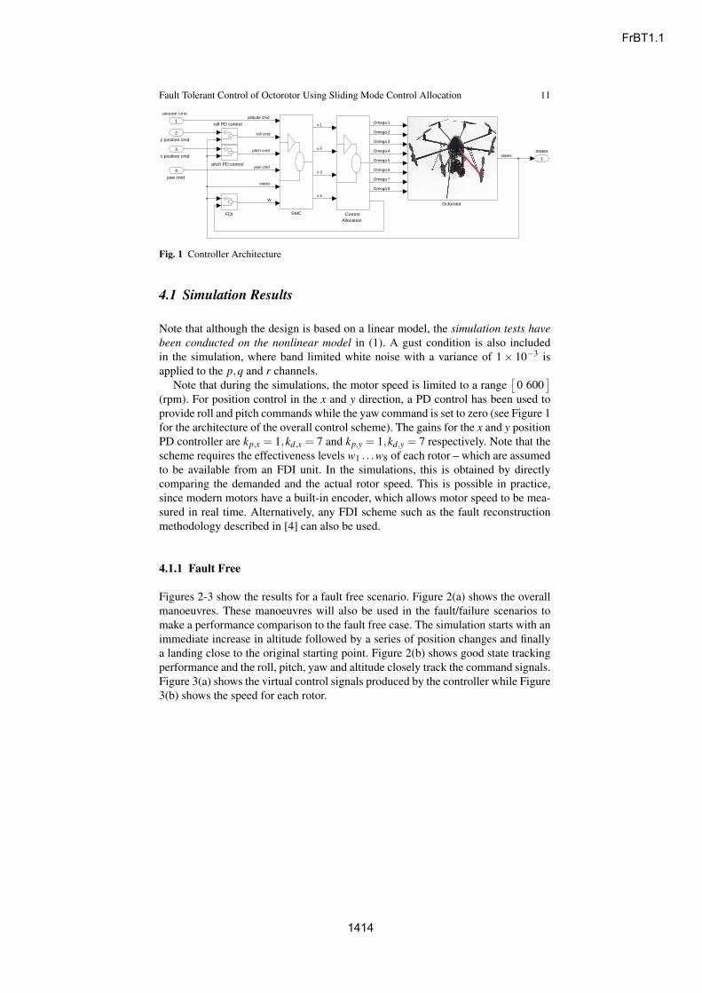
Fig. 1 Controller Architecture

4.1 Simulation Results

Note that although the design is based on a linear model, the simulation tests havebeen conducted on the nonlinear model in (1). A gust condition is also includedin the simulation, where band limited white noise with a variance of 1× 10−3 isapplied to the p,q and r channels.

Note that during the simulations, the motor speed is limited to a range[

0 600]

(rpm). For position control in the x and y direction, a PD control has been used toprovide roll and pitch commands while the yaw command is set to zero (see Figure 1for the architecture of the overall control scheme). The gains for the x and y positionPD controller are kp,x = 1,kd,x = 7 and kp,y = 1,kd,y = 7 respectively. Note that thescheme requires the effectiveness levels w1 . . .w8 of each rotor – which are assumedto be available from an FDI unit. In the simulations, this is obtained by directlycomparing the demanded and the actual rotor speed. This is possible in practice,since modern motors have a built-in encoder, which allows motor speed to be mea-sured in real time. Alternatively, any FDI scheme such as the fault reconstructionmethodology described in [4] can also be used.

4.1.1 Fault Free

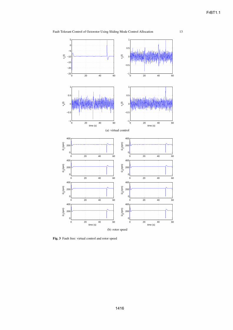
Figures 2-3 show the results for a fault free scenario. Figure 2(a) shows the overallmanoeuvres. These manoeuvres will also be used in the fault/failure scenarios tomake a performance comparison to the fault free case. The simulation starts with animmediate increase in altitude followed by a series of position changes and finallya landing close to the original starting point. Figure 2(b) shows good state trackingperformance and the roll, pitch, yaw and altitude closely track the command signals.Figure 3(a) shows the virtual control signals produced by the controller while Figure3(b) shows the speed for each rotor.

FrBT1.1

1414


00.2

0.40.6

0.81

1.2

0

0.2

0.4

0.6

0.8

1

1.20

1

2

3

4

5

6

xb (m)y

b (m)

altit

ude

(m)

(a) 3d manoeuvre

0 20 40 60−0.5

0

0.5

1

1.5

x b (m

)

0 20 40 60−0.5

0

0.5

1

1.5

y b (m

)

0 20 40 60−2

0

2

4

6

altit

ude

(m)

time (s)

0 20 40 60

−5

0

5

φ (d

eg)

0 20 40 60

−5

0

5

θ (d

eg)

0 20 40 60−1

−0.5

0

0.5

1

ψ (

deg)

time (s)

actualcmd

(b) states

Fig. 2 Fault free: position and states

FrBT1.1

1415


0 20 40 60−25

−20

−15

−10

−5

0

5

ν 1(t)

0 20 40 60−1

−0.5

0

0.5

1

ν 2(t)

0 20 40 60−1

−0.5

0

0.5

1

ν 4(t)

time (s)0 20 40 60

−1

−0.5

0

0.5

1

ν 4(t)

time (s)

(a) virtual control

0 20 40 60

0

200

400

Ω1(r

pm)

0 20 40 60

0

200

400

Ω2(r

pm)

0 20 40 60

0

200

400

Ω3(r

pm)

0 20 40 60

0

200

400

Ω4(r

pm)

0 20 40 60

0

200

400

Ω5(r

pm)

0 20 40 60

0

200

400

Ω6(r

pm)

0 20 40 60

0

200

400

Ω7(r

pm)

time (s)0 20 40 60

0

200

400

Ω8(r

pm)

time (s)

(b) rotor speed

Fig. 3 Fault free: virtual control and rotor speed

FrBT1.1

1416


4.1.2 Rotor 2,4,6,8 failure

Figure 4(b) shows the rotor speeds when rotors 2, 4, 6 and 8 are totally failed after20sec during a change in the xb position. Figure 4(a) shows the states of both thefault free and failure cases, to show the difference between the two cases. It can beseen that despite the failure to 4 rotors, there is no visible change in terms of theperformance (lines overlap), thus highlighting the efficacy of the proposed scheme.Note that compared to [2], the scheme proposed here can deal with more than onesingle rotor failure, by taking advantage of the available redundancy through controlallocation.


Figure 5 shows simulation results when a different set of rotors (rotor 1, 4, 6 and 7)fail at 20 sec. Figure 5(b) clearly shows the speed of rotors 1, 4, 6 and 7 has droppedto zero at 20 sec – which simulates the failure. The control signal is redistributed torotors 2, 3, 5 and 7 which show an increase in speed in order to compensate for thefailed rotors. Again Figure 5(a) shows no visible degradation in performance whencompared to the fault free case (the lines overlap) which highlights the efficacy ofthe proposed scheme.


Figure 6 shows the effect when rotors 1, 3, 5 and 7 fail at different times duringthe manoeuvre. Figure 6(b) shows rotors 1, 3, 5, 7 fail at 20, 30, 40 and 50 secrespectively. It can be seen that the rotor speed for rotors 2, 4, 6, 8 increases tocompensate for the effect of rotor failures. Figure 6(a) shows no visible differencein terms of state tracking performance (the lines overlap) despite the failure of 4 ofthe rotors.

4.1.5 Rotor 2,4,6,8 fault and rotor 1,3 failure

Figure 7(b) shows a more severe fault/failure scenario where rotors 2, 4, 6 and 8 areonly 50% effective from 20 sec onwards, and then rotor 1 and 3 fail totally at 30sec.Despite the fact that 4 rotors are only 50% effective and 2 rotors have totally failed,Figure 7(a) shows no visible difference in terms of state performance compared tothe fault free case (lines overlap), and thus the proposed scheme has managed tomaintain fault free performance.

FrBT1.1

1417


0 20 40 60−0.5

0

0.5

1

1.5

x b (m

)

0 20 40 60−0.5

0

0.5

1

1.5

y b (m

)

0 20 40 60−2

0

2

4

6

altit

ude

(m)

time (s)

0 20 40 60−4

−2

0

2

4

φ (d

eg)

0 20 40 60−5

0

5

θ (d

eg)

0 20 40 60−1

−0.5

0

0.5

1

ψ (

deg)

time (s)

failure casefault free

(a) states

0 20 40 60

0

200

400

Ω1(r

pm)

0 20 40 60

0

200

400

Ω2(r

pm)

0 20 40 60

0

200

400

Ω3(r

pm)

0 20 40 60

0

200

400

Ω4(r

pm)

0 20 40 60

0

200

400

Ω5(r

pm)

0 20 40 60

0

200

400

Ω6(r

pm)

0 20 40 60

0

200

400

Ω7(r

pm)

time (s)0 20 40 60

0

200

400

Ω8(r

pm)

time (s)


(b) rotor speed

Fig. 4 Rotor 2,4,6,8 failure

FrBT1.1

1418


0 20 40 60−0.5

0

0.5

1

1.5

x b (m

)

0 20 40 60−0.5

0

0.5

1

1.5

y b (m

)

0 20 40 60−2

0

2

4

6

altit

ude

(m)

time (s)

0 20 40 60−4

−2

0

2

4

φ (d

eg)

0 20 40 60−5

0

5

θ (d

eg)

0 20 40 60−1

−0.5

0

0.5

1

ψ (

deg)

time (s)


(a) states

0 20 40 60

0

200

400

Ω1(r

pm)

0 20 40 60

0

200

400

Ω2(r

pm)

0 20 40 60

0

200

400

Ω3(r

pm)

0 20 40 60

0

200

400

Ω4(r

pm)

0 20 40 60

0

200

400

Ω5(r

pm)

0 20 40 60

0

200

400

Ω6(r

pm)

0 20 40 60

0

200

400

Ω7(r

pm)

time (s)0 20 40 60

0

200

400

Ω8(r

pm)

time (s)


(b) rotor speed

Fig. 5 Rotor 1,4,6,7 failure

FrBT1.1

1419


0 20 40 60−0.5

0

0.5

1

1.5

x b (m

)

0 20 40 60−0.5

0

0.5

1

1.5

y b (m

)

0 20 40 60−2

0

2

4

6

altit

ude

(m)

time (s)

0 20 40 60−4

−2

0

2

4

φ (d

eg)

0 20 40 60−5

0

5

θ (d

eg)

0 20 40 60−1

−0.5

0

0.5

1

ψ (

deg)

time (s)


(a) states

0 20 40 60

0

200

400

Ω1(r

pm)

0 20 40 60

0

200

400

Ω2(r

pm)

0 20 40 60

0

200

400

Ω3(r

pm)

0 20 40 60

0

200

400

Ω4(r

pm)

0 20 40 60

0

200

400

Ω5(r

pm)

0 20 40 60

0

200

400

Ω6(r

pm)

0 20 40 60

0

200

400

Ω7(r

pm)

time (s)0 20 40 60

0

200

400

Ω8(r

pm)

time (s)


(b) rotor speed

Fig. 6 Rotor 1,3,5,7 failure at different time

FrBT1.1

1420


0 20 40 60−0.5

0

0.5

1

1.5

x b (m

)

0 20 40 60−0.5

0

0.5

1

1.5

y b (m

)

0 20 40 60−2

0

2

4

6

altit

ude

(m)

time (s)

0 20 40 60−4

−2

0

2

4

φ (d

eg)

0 20 40 60−5

0

5

θ (d

eg)

0 20 40 60−1

−0.5

0

0.5

1

ψ (

deg)

time (s)


(a) states

0 20 40 60

0

200

400

Ω1(r

pm)

0 20 40 60

0

200

400

Ω2(r

pm)

0 20 40 60

0

200

400

Ω3(r

pm)

0 20 40 60

0

200

400

Ω4(r

pm)

0 20 40 60

0

200

400

Ω5(r

pm)

0 20 40 60

0

200

400

Ω6(r

pm)

0 20 40 60

0

200

400

Ω7(r

pm)

time (s)0 20 40 60

0

200

400

Ω8(r

pm)

time (s)


(b) rotor speed

Fig. 7 Rotor 2,4,6,8 fault and rotor 1,3 failure

FrBT1.1

1421


5 Conclusions

This paper has presented a sliding mode control allocation scheme for an octorotor.The scheme takes full advantage of the redundant rotors to handle more than onerotor failure as compared to the existing literature. The core controller is based ona sliding mode design which is robust against faults and uncertainty in the inputchannels (matched uncertainty). When a fault/failure occurs, no reconfiguration isrequired and the control effort to the faulty rotors is re-allocated to the healthy onesusing control allocation. Simulation results show no visible change in performance(as compared to the fault free case) for various types of fault/failure scenarios, high-lighting the efficacy of the proposed scheme.

References

1. V.G. Adır and A.M. Stoica. Integral LQR control of a star-shaped octorotor. INCAS Bulletin,4(2):3–18, 2012.

2. V.G. Adır, A.M. Stoica, A. Marks, and J.F. Whidborne. Modelling, stabilization and singlemotor failure recovery of a 4Y octorotor. In 13th IASTED International Conference on Intel-ligent Systems and Control (ISC 2011), Cambridge, U.K, 2011.

3. H. Alwi and C. Edwards. Fault tolerant control using sliding modes with on-line controlallocation. Automatica, 44(7):1859–1866, 2008.

4. H. Alwi, C. Edwards, and C. P. Tan. Fault Detection and Fault–Tolerant Control Using SlidingModes. Advances in Industrial Control. Springer-Verlag, 2011.

5. C. Balas. Modelling and linear control of a quadrotor. Master of Science Thesis, School ofEngineering, Cranfield, 2007.

6. S. Bouabdallah. Design and control of quadrotors with application to autonomous flying. PhDthesis, Ecole Polytechnique Federale De Lausanne, 2007.

7. S. Bouabdallah and R. Siegwart. Backstepping and sliding-mode techniques applied to anindoor micro quadrotor. In International Conference on Robotics and Automation, Barcelona,Spain, 2005.

8. G. Ducard and M-D Hua. Discussion and practical aspects on control allocation for a multi-rotor helicopter. In 1st International Conference on UAVs in Geomatics, UAV-g 2011, Zurich,Switzerland, 2011.

9. C. Edwards, T. Lombaerts, and H. Smaili (Eds.). Fault Tolerant Flight Control: A BenchmarkChallenge, volume 399. Springer-Verlag: Lecture Notes in Control and Information Sciences,2010.

10. C. Edwards and S. K. Spurgeon. Sliding Mode Control: Theory and Applications. Taylor &Francis, 1998.

11. A. Freddi, A. Lanzon, and A. Longhi. A feedback linearization approach to fault tolerance inquadrotor vehicles. In Proceedings of the 18th IFAC World Congress, Milan, 2011.

12. M. Hamayun, H. Alwi and C. Edwards, An LPV Fault Tolerant Control Scheme Using IntegralSliding Modes 51st IEEE Conference on Decision and Control, Maui, Hawaii, 2012.

13. O. Harkegard and S. T. Glad. Resolving actuator redundancy - optimal control vs. controlallocation. Automatica, 41(1):137–144, 2005.

14. H. A. Izadi, Y. Zhang, and B. W. Gordon. Fault tolerant model predictive control of quad-rotorhelicopters with actuator fault estimation. In Proceedings of the 18th IFAC World Congress,Milan, 2011.

15. M. Labadille. Non-linear control of a quadrotor. Master of Science Thesis, School of Engi-neering, Cranfield, 2007.

FrBT1.1

1422


16. T. Madani and A. Benallegue. Backstepping sliding mode control applied to a miniaturequadrotor flying robot. In 32nd IEEE Conference on Industrial Electronics, IECON, 2006.

17. T. Madani and A. Benallegue. Control of a quadrotor mini-helicopter via full state back-stepping technique. In 45th IEEE Conference on Decision and Control,San Diego, CA, USA,2006.

18. T. Madani and A. Benallegue. Sliding mode observer and backstepping control for a quadrotorunmanned aerial vehicles. In American Control Conference, New York City, USA,, 2007.

19. V. M. Martınez. Modelling of the flight dynamics of a quadrotor helicopter. Master of ScienceThesis, School of Engineering, Cranfield, 2007.

20. I. Sadeghzadeh, A. Mehta, Y. Zhang, and C. Rabbath. Fault-tolerant trajectory tracking controlof a quadrotor helicopter using gain-scheduled pid and model reference adaptive control. InConference of the Prognostics and Health Management Society, 2011.

21. A.S. Sanca, P.J. Alsina, and J.d.J.F. Cerqueira. Dynamic modeling with nonlinear inputs andbackstepping control for a hexarotor micro-aerial vehicle. In Latin American Robotics Sym-posium and Intelligent Robotics Meeting, 2010.

22. T. Schneider, G. Ducard, K. Rudin, and P. Strupler. Fault-tolerant control allocation for mul-tirotor helicopters using parametric programming. In International Micro Air Vehicle Confer-ence and Flight Competition, Braunschweig, Germany, 2012.

23. F. Sharifi, M. Mirzaei, B.W. Gordon, and Y. Zhang. Fault tolerant control of a quadrotoruav using sliding mode control. In Conference on Control and Fault Tolerant Systems, Nice,France, 2010.

24. B. R. Trilaksono, R. Triadhitama, W. Adiprawita, A. Wibowo, and A. Sreenatha. Hardware-in-the-loop simulation for visual target tracking of octorotor UAV. Aircraft Engineering andAerospace Technology: An International Journal, 83(6):407–419, 2011.

25. V. I. Utkin. Sliding Modes in Control Optimization. Springer-Verlag, Berlin, 1992.26. R. Xu and U. Ozguner. Sliding mode control of a quadrotor helicopter. In 45th IEEE Confer-

ence on Decision and Control,San Diego, CA, USA, 2006.27. L. Yin, J. Shi, and Y. Huang. Modeling and control for a six-rotor aerial vehicle. In Interna-

tional Conference on Electrical and Control Engineering, 2010.28. Y. Zhang and A. Chamseddine. Fault tolerant flight control techniques with application to a

quadrotor UAV testbed. In T. Lombaerts, editor, Automatic Flight Control Systems - LatestDevelopments, pages 119–150. InTech, 2012.

FrBT1.1

1423

fault tolerant control of octorotor using sliding mode ... · 3 sliding mode control synthesis 3.1...

Documents