Fachbereich Informatik

Diplomarbeit

Support Vector Machines in der digitalen Mustererkennung

Ausgeführt bei der FirmaSiemens VDO in Regensburg

vorgelegt von: Christian MiklosSt.-Wolfgangstrasse 1193051 Regensburg

Betreuer: Herr Reinhard RöslErstprüfer: Prof. Jürgen SauerZweitprüfer: Prof. Dr. Herbert Kopp

Abgabedatum: 03.03.2004

2

Acknowledgements

This work was written as my diploma thesis in computer science at the university of applied sciences Regensburg, Germany, under the supervi-sion of Prof. Dr. Jürgen Sauer.

The research was carried out at Siemens VDO in Regensburg, Germany.In Reinhard Rösl I found a very competent advisor there, whom I owe much for his assistance in all aspects of my work. Thank you very much !

For the help during writing this document I want to thank all colleagues at the department at Siemens VDO.I have enjoyed the work there very much in any sense and learned a lot which sure will be useful in the upcoming years.

My special thanks go to Prof. Jürgen Sauer who helped me out in any questions arising during this work.

1

CONTENTS

ABSTRACT 5

NOTATIONS 6

0 INTRODUCTION 7

I AN INTRODUCTION TO THE LEARNING THEORY AND BASICS 9

1 SUPERVISED LEARNING THEORY 10

1.1 Modelling the Problem 11

2 LEARNING TERMINOLOGY 14

2.1 Risk Minimization 142.2 Structural Risk Minimization (SRM) 162.3 The VC Dimension 172.4 The VC Dimension of Support Vector Machines, Error Estimation and Generaliza-

tion Ability 18

3 PATTERN RECOGNITION 21

3.1 Feature Extraction 223.2 Classification 22

4 OPTIMIZATION THEORY 25

4.1 The Problem 254.2 Lagrangian Theory 294.3 Duality 324.4 Kuhn-Tucker Theory 33

II SUPPORT VECTOR MACHINES 35

5 LINEAR CLASSIFICATION 36

5.1 Linear Classifiers on Linear Separable Data 365.2 The Optimal Separating Hyperplane for Linear Separable Data 39

5.2.1 Support Vectors 465.2.2 Classification of unseen data 49

5.3 The Optimal Separating Hyperplane for Linear Non-Separable Data 505.3.1 1-Norm Soft Margin - or the Box Constraint 525.3.2 2-Norm Soft Margin - or Weighting the Diagonal - 54

5.4 The Duality of Linear Machines 57

5.5 Vector/Matrix Representation of the Optimization Problem and Summary 58

2

5.5.1 Vector/Matrix Representation 585.5.2 Summary 59

6 NONLINEAR CLASSIFIERS 63

6.1 Explicit Mappings 646.2 Implicit Mappings and the Kernel Trick 69

6.2.1 Requirements for Kernels - Mercer’s Condition - 726.2.2 Making Kernels from Kernels 736.2.3 Some well-known Kernels 74

6.3 Summary 78

7 MODEL SELECTION 80

7.1 The RBF Kernel 807.2 Cross Validation 81

8 MULTICLASS CLASSIFICATION 82

8.1 One-Versus-Rest (OVR) 828.2 One-Versus-One (OVO) 848.3 Other Methods 87

III IMPLEMENTATION 88

9 IMPLEMENTATION TECHNIQUES 89

9.1 General Techniques 899.2 Sequential Minimal Optimization (SMO) 90

9.2.1 Solving for two Lagrange Multipliers 929.2.2 Heuristics for choosing which Lagrange Multipliers to optimize 1009.2.3 Updating the threshold b and the Error Cache 1019.2.4 Speeding up SMO 1039.2.5 The improved SMO algorithm by Keerthi 1059.2.6 SMO and the 2-norm case 106

9.3 Data Pre-Processing 1079.3.1 Categorical Features 1079.3.2 Scaling 108

9.4 Matlab Implementation and Examples 1089.4.1 Linear Kernel 1099.4.2 Polynomial Kernel 1119.4.3 Gaussian Kernel (RBF) 1139.4.4 The Impact of the Penalty Parameter C on the Resulting Classifier

and the Margin 118

IV MANUALS, AVAILABLE TOOLBOXES AND SUMMARY 122

10 MANUAL 123

10.1 Matlab Implementaion 12310.2 Matlab Examples 12610.3 The C++ Implementation for the Neural Network Tool 13210.4 Available Toolboxes implementing SVM 13710.5 Overall Summary 138

LIST OF FIGURES 140

3

LIST OF TABLES 142

LITERATURE 143

STATEMENT 145

APPENDIX 146

A SVM - APPLICATION EXAMPLES 146

A.1 Hand-written Digit Recognition 146A.2 Text Categorization 147

B LINEAR CLASSIFIERS 148

B.1 The Perceptron 148

C CALCULATION EXAMPLES 154

D SMO PSEUDO CODES 159

D.1 Pseudo Code of original SMO 159D.2 Pseudo Code of Keerthi’s improved SMO

161

4

ABSTRACT

The Support Vector Machine (SVM) is a new and very promising classific-ation technique developed by Vapnik and his group at AT&T Bell Laborat-ories. This new learning algorithm can be seen as an alternative training technique for Polynomial, Radial Basis Function and Multi-Layer Per-ceptron classifiers. Recently it has shown very good results in the pattern recognition field of research, such as hand-written character and digit or face recognition but they also proofed themselves reliable in text categor-ization. It is mathematically very funded and of great growing interest nowadays in many new fields of research such as Bioinformatics.

Die Support Vector Machine (SVM) ist eine neue und sehr vielversprechende Klassifizierungs-Methode, entwickelt von Vapnik und seiner Gruppe in den AT&T Bell Forschungseinrichtungen. Dieser neue Ansatz im Bereich des computergestützten Lernens kann als alternative Trainingstechnik für Polynom-, Gaußkern- und Multi-Layer Perzeptron-Klassifizierer aufgefasst werden. In jüngster Zeit zeigte diese neue Technik sehr gute Ergebnisse im Bereich der Mustererkennung, wie z.B. Erkennung von handschriftlichen Buchstaben und Zahlen oder Gesichtszügen. Desweiteren wurde sie auch zuverlässig im Bereich der Textkategorisierung eingesetzt. Die Technik ist mathematisch sehr gut fundiert und von immer wachsenderem Interesse in neueren Forschungsgebieten, wie der Bioinformatik.

5

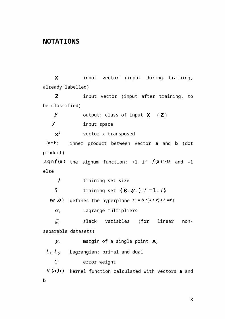
NOTATIONS

input vector (input during training, already labelled)

input vector (input after training, to be classified)

output: class of input ( )

input space

vector x transposed

inner product between vector a and b (dot product)

the signum function: +1 if and -1 else

training set size

training set

defines the hyperplane

Lagrange multipliers

slack variables (for linear non-separable datasets)

margin of a single point

Lagrangian: primal and dual

error weight

kernel function calculated with vectors a and b

kernel matrix ( )

Support Vector Machine

support vectors

number of support vectors

radial basis functions

learning machine

Empirical Risk Minimization

Structural Risk Minimization

6

Chapter 0

Introduction

In this work the rather new concept in learning theory, the Support Vector Machine, will be discussed in detail. The goal of this work is to give an in-sight into the methods used and to describe them in a way a person with not so much funded mathematical background could understand them. So the gap between theory and practice could be closed. It is not the intention of this work to look in every aspect and algorithm available in the field of this learning theory but to understand how and why it even works and why it is of such rising interest at the time.This work should lay the basics for understanding the mathematical back-ground, to be able to implement the technique and to do further research whether this technique is suitable for the wanted purpose at all. As a product of this work the Support Vector Machine will be implemented both in Matlab and C++. The C++ part will be a module integrated into the so called “Neural Network Tool” already used in the department at Siemens VDO, which already implements the Polynomial and Radial-Basis Function classifiers. This tool is for testing purposes to test suitable techniques for the later integration into the lane recognition system for cars currently under development there.

Support Vector Machines for classification are a rather new concept in learning theory. It’s origins reach back to the early 60’s (VAPNIK and LEARNER 1963; VAPNIK and CHERVONENKIS 1964), but it stirred up attention only in 1995 with Vladimir Vapnik’s book The Nature of Statistical Learning Theory [Vap95]. In the last few years Support Vector Machines proofed excellent performance in many real-word applications such as hand-written character recognition, image classification or text categoriza-tion.

But because many aspects in this theory are still under intensive research the number of introductory literature is very limited. The two books by Vladimir Vapnik (The Nature of Statistical Learning Theory [Vap 95] and Statistical Learning Theory [Vap98] present only a general high-level intro-duction to this field. The first tutorial purely on Support Vector Machines was written by C. Burges in 1998 [Bur98]. In the year 2000 CHRISTIANINI and SHAWE-TAYLOR published An introduction to Support Vector Ma-chines [Nel00], which was the main source for this work.

7

All these books and papers give a good overview of the theory behind Support Vector Machines, but they don’t give a straightforward introduc-tion to application. Here this work puts on.

This work is divided into four parts:

Part I gives an introduction into the supervised learning theory and the ideas behind pattern recognition. Pattern recognition is the environment in which the Support Vector Machine will be used in this work. The next chapter will lay the mathematical basics for the optimization problem arising.

Part II then introduces the Support Vector Machine itself with its’ mathem-atical background. For a better understanding the case of classification will be restricted to the two-class problem first but later one can see that this is no problem because it then can easily be extended to the multi-class case. Here also the long studied kernel technique will be analysed in detail which gives the Support Vector Machines their superior power.

Part III then analyses the implementation techniques for Support Vector Machines. It will be shown that there are many approaches for solving the arising optimization problem but only the most used and best performing algorithms for a great amount of data will be discussed in detail.

Part IV in the end is intended as a manual for the implementation done in Matlab and C++. There will also be given a list of widely used toolboxes for Support Vector Machines, both in C/C++ and Matlab.

Last but not least in the appendix some real-world applications, some cal-culation examples on the arising mathematical problems, the rather simple Perceptron algorithm for classification and the pseudo code used for the implementation will be stated.

8

Part I

An introduction to the Learning Theory and Basics

9

Chapter 1

Supervised Learning Theory

When computers are applied to solve a practical problem it is usually the case that the method of deriving the required output from a set of inputs can be described explicitly. But there arise many cases where one wants the machine to perform tasks that cannot be described by an algorithm. Such tasks cannot be solved by classical programming techniques, since no mathematical model exists for them or the computation of the exact solution is very expensive (it could last for hundreds of years, even on the fastest processors). As examples consider the problem of performing hand-written digit recognition (a classical problem of machine learning) or the detection of faces on a picture.

There is need for a different approach to solve such problems. Maybe the machine is teachable, as children are in school ? Meaning they are not given abstract definitions and theories by the teacher but he points out ex-amples of the input-output functionality. Consider the children learning the alphabet. The teacher does not give them precise definitions of each let-ter, but he shows them examples. Thereby the children learn general properties of the letters by examining these examples. In the end these children will be able to read words in script style, even if they were taught only on types. In other more mathematical words this observations leads to the concept of classifiers. The purpose of learning such a classifier from few given ex-amples already correctly classified by the supervisor, is to be able to clas-sify future unknown observations correctly.

But how can learning from examples, which is called supervised learning, be formulized mathematically to let it be applied to a machine ?

10

1.1 Modelling the Problem

Learning from examples can be described in a general model by the fol-lowing elements:The generator of the input data x, the supervisor who assigns labels/classes y to the data for learning and the learning machine that returns some answer y’ hopefully close to the one of the supervisor.

The labelled/preclassified examples (x, y) are referred to as the training data. The input/output pairings typically reflect a functional relationship, mapping the inputs to outputs, though this is not always the case, for ex-ample when the outputs are corrupted by noise. But when an underlying function exists it is referred to as the target function. So the goal is the es-timation of this target function which is learnt by the learning machine and is known as the solution of the learning problem. In case of classification problems, e.g. “this is a man and this is a woman”, this function is also known as the decision function. The optimal solution is chosen from a set of candidate functions which map from the input space to the output do-main. Usually a set or class of candidate functions is chosen known as hy-potheses. As an example consider so-called decision trees which are hy-potheses created by constructing a binary tree with simple decision func-tions at the internal nodes and output values at the leaves (the y-values). A learning problem with binary outputs (0/1, yes/no, positive/negative, …) is referred to as a binary classification problem, one with a finite number of categories as a multi-class classification one, while for real-valued out-puts the problem is known as regression. In this diploma thesis only the first two categories will be considered, although the later discussed Sup-port Vector Machines can be “easily” extended to the regression case.

A more mathematical interpretation of this will be given now. The generator above determines the environment in which the supervisor and the learning machine act. It generates the vectors independ-ently and identically distributed according to some unknown probability distribution P(x).

The supervisor assigns the “true” output values according to a conditional distribution function P(y| x) (output is dependent on input). This assump-tion leads to the case y = f(x) in which the supervisor associates a fixed y with every x.

The learning machine then is defined by a set of possible mappings where is element of a parameter space. An example of a

learning machine according to binary classification is defined by oriented hyperplanes where determines the posi-

11

tion of the hyperplanes in . As a result the following learning machine (LM) is obtained:

1

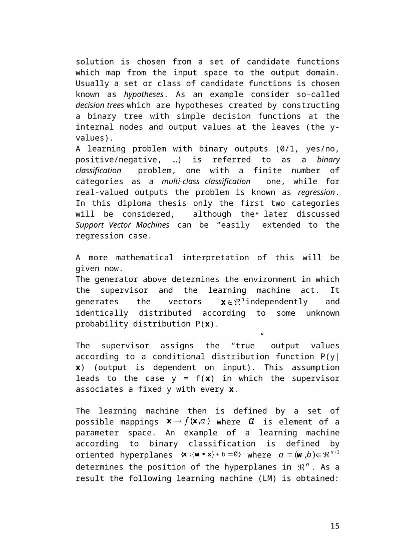
The functions , mapping the input x to the positive (+1) or negative (-1) class, are called the decision functions. So this learning ma-chine works as follows: the input x is assigned to the positive class, if f(x)

0, and otherwise to the negative class.

Figure 1.1: Multiple possible decision functions in the . They are defined as

(for details see part II of this work). Points to the left are assigned to the

positive (+1)class, and the ones to the right to the negative (-1) class,

The above definition of a learning machine is called a Linear Learning Ma-chine because of the linear nature of the function f used here. Among all possible functions, the linear ones are the best understood and simplest to apply. They will provide the framework within which the construction of more complex systems is possible and will be done in later chapters.

There is need for a choice of the parameter based on l observations (the training set):

1 This method of a learning machine will be described in detail in Part II, because Support

Vector Machines implement this technique.

12

This is called the training of the machine. The training set S is drawn ac-cordingly to the distribution P(x, y). If all this data is given to the learner (the machine) at the start of the learn -ing phase, this is called batch learning. But if the learner receives only one example at a time and gives an estimation of the output before receiving the correct value, it is called online learning. In this work only batch learn-ing is considered. Also each of these two learning methods can be sub-divided into unsupervised learning and supervised learning.

Once a function for appropriate mapping the input to the output is chosen (learned), one wants to see how well it works on unseen data. Usually the training set is split into two parts: the labelled training set above and the so-called labelled test set. This test set is applied after training, knowing the expected output values, and comparing the results of the classification of the machine with the expected ones to gain the error rate of the ma-chine.

But simply verifying the quality of an algorithm in such a way is not enough. It is not only the goal of a gained hypothesis to be consistent with the training set but also to work fine on future data. But there are also other problems inside the whole process of generating a verifiable consist-ent hypothesis. First the function tried to learn may have not a simple rep-resentation and hence may not be easily verified in this way. Second the training data could be frequently noisy and so there is no guarantee that there is an underlying function which correctly maps the training data. But the main problem arising in practice is the choice of the features. Fea-tures are the components the input vector x consists of. Sure they have to describe the input data for classification in an “appropriate” way. Appropri-ate means, for example, no or less redundancy. Some hints on choosing a suitable representation for the data will be given in the upcoming chapters but not in detail because this would blow up the frame. As an example to the second problem consider the classification of web pages into categories, which can never be an exact science. But such data is increasingly of interest for learning. So there is a need for measur-ing the quality of a classifier in some other way: Good generalization.

The ability of a hypothesis/classifier to correctly classify data, not only the training set, or in other words, make precise predictions by learning from few examples, is known as its generalization ability, and this is the prop-erty which has to be optimized.

13

Chapter 2

Learning Terminology

This chapter is intended to stress the main concepts arising from the the-ory of statistical learning [Vap79] and the VC Theory [Vap95]. These con-cepts are the fundamentals of learning machines. Here terms such as generalization ability and capacity will be described.

2.1 Risk Minimization

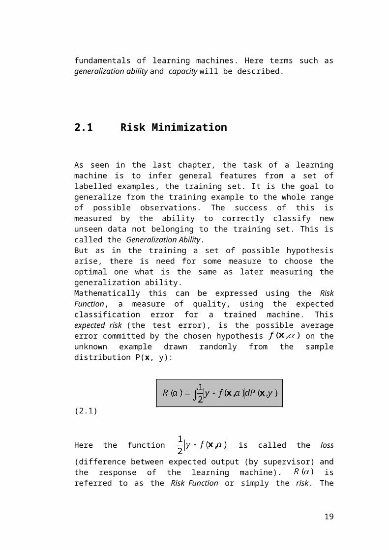
As seen in the last chapter, the task of a learning machine is to infer gen-eral features from a set of labelled examples, the training set. It is the goal to generalize from the training example to the whole range of possible ob-servations. The success of this is measured by the ability to correctly clas-sify new unseen data not belonging to the training set. This is called the Generalization Ability. But as in the training a set of possible hypothesis arise, there is need for some measure to choose the optimal one what is the same as later meas-uring the generalization ability.Mathematically this can be expressed using the Risk Function, a measure of quality, using the expected classification error for a trained machine. This expected risk (the test error), is the possible average error committed by the chosen hypothesis on the unknown example drawn ran-domly from the sample distribution P(x, y):

(2.1)

Here the function is called the loss (difference between ex-

pected output (by supervisor) and the response of the learning machine). is referred to as the Risk Function or simply the risk. The goal is to

find parameters such that minimizes the risk over the class of

14

functions . But since P(x, y) is unknown, the value of the risk for a given parameter cannot be computed directly. The only available inform-ation is contained in the given training set S.So the empirical risk is defined to be just the measured mean er-ror rate on the training set of finite length l:

(2.2)

Note that here no probability distribution appears and is a fixed number for a particular choice of and for a training set S.For further considerations, assume binary classification with outputs

. Then the loss function can only produce the outputs 0 or 1. Now choose some such that . Then for losses taking these val-ues, with probability , the following bound holds [Vap95]:

(2.3)

where h is a non-negative integer called the Vapnik Chervonenkis (VC) di-mension. It is a measure of the notion of capacity. The second summand of the right hand side is called the VC confidence.

Capacity is the ability of a machine to learn any training set without error. It is a measure of the richness or flexibility of the function class. A machine with too much capacity tends to overfitting, whereas low capa-city leads to errors on the training set. The most popular concept to de-scribe the richness of a function class in machine learning is the Vapnik Chervonenkis (VC) dimension.

Burges gives an illustrative example on capacity in his paper [Bur98]: “A machine with too much capacity is like a botanist with a photographic memory who, when presented with a new tree, concludes that it is not a tree because it has a different number of leaves from anything he has seen before. A machine with too little capacity is like the botanist’s lazy brother, who declares that if it is green, it is a tree. Neither can generalize well.” To conclude this subchapter there can be drawn three key points about the bound of (2.3):

15

First it is independent of the distribution P(x, y). It only assumes that the training and test data are drawn independently according to some distribu-tion P(x, y). Second, it is usually not possible to compute the left hand side. Third, if h is known, it is easily possible to compute the right hand side. The bound also shows that low risk depends both on the chosen class of functions (the learning machine) and on the particular function chosen by the learning algorithm, the hypothesis, which should be optimal. The bound decreases if a good separation on the training set is achieved by a learning machine with low VC dimension. This approach leads to prin-ciples of the structural risk minimization (SRM).

2.2 Structural Risk Minimization (SRM)

Let the entire class of functions , be divided into nested sub-sets of functions such that . For each subset it must be able to compute the VC dimension h, or get a bound on h itself. Then SRM consists of finding that subset of functions which minimizes the bound on the risk. This can be done by simply training a series of ma-chines, one for each subset, where for a given subset the goal of training is simply to minimize the empirical risk. Then the trained machine in the series whose sum of empirical risk and VC confidence is minimal.

So overall the approach is working as follows: The confidence interval is kept fix (by choosing particular h’s) and the empirical risk is minimized. In the neural network case this technique is adapted by first choosing an ap-propriate architecture and then eliminating classification errors. The second approach is to keep the empirical risk fixed (e.g. equal to zero) and minimize the confidence interval. Support Vector Machines will also imple-ment the principles of SRM, by finding the one canonical hyperplane among all, which minimizes the norm in the definition of a hyperplane by: .2

2.3 The VC Dimension

The VC dimension is a property of a set of functions and can be defined for various classes of functions f. But again, here only the func-

2 SVMs, hyperplanes, canonical hyperplanes and why minimizing the norm will be ex-

plained in part II of this work in detail, here only a reference is given to this.

16

tions corresponding to the two-class pattern case with are considered.

Definition 2.1 (Shattering)

If a given set of l points can be labelled in all possible 2 lways, and for each labelling, a member of the set can be found which correctly assigns those labels (classifies), this set of points is said to be shattered by that set of functions.

Definition 2.2 (VC Dimension)

The Vapnik Chervonenkis (VC) Dimension of a set of functions is defined as the maximum number of training points that can be shattered by it. The VC dimension is infinite, if l points can be shattered by the set of functions, no matter how large l is.

Note that if the VC dimension is h, then there exists at least one set of h points that can be shattered, but in general it will not be true that every set of h points can be shattered.

As an example consider shattering points with oriented hyperplanes in . To give an introduction assume the data lives in the space and the set of functions consists of oriented straight lines, so that for a given line, all points on one side are assigned to the class +1, and all points on the other one to the class -1. The orientation in the following figures is in-dicated by an arrow, specifying the side where the points of class +1 are lying. While it is possible to find three points that can be shattered (figure 2.1) by this set of functions, it is not possible to find four. Thus the VC di-mension of the set of oriented lines in the is three. Without proof (this can be found in [Bur98]) it can be stated that the VC di-mension of the set of oriented hyperplanes in the is n+1.

17

Figure 2.1: Three points not lying in a line can be shattered by oriented hyperplanes in

the . The arrow points in the direction of the positive examples (black). Whereas four

points can be found in the , which cannot be shattered by oriented hyperplanes.

2.4 The VC Dimension of Support Vector Ma-chines, Error Estimation and Generaliza-tion Ability

It should be said first that this subchapter does not claim completeness in any sense. There will be no proofs on the conclusions stated and the con-tents written are only excerpts of the theory. This is because the theory stated here is beyond the intention of this work. The interested reader can refer to the books about the Statistical Learning Theory [Vap79] , VC The-ory [Vap95] and many other works on this. Here only some important sub-sets for Support Vector Machines of the whole theory will be shown.

Imagine points in the , which should be binary classified: class +1 or class -1. They are consistent with many classifiers (hypothesises, set of

18

functions). But how can one minimize the room of the hypothesis set ? One approach is to apply a margin to each data point (figures 1.1 and 2.2), then, the broader that margin, the smaller the room for hypotheses is. This approach is justified by Vapnik’s learning theory.

Figure 2.2: Reducing the room for hypothesis by applying a margin to each point

Therefore the later introduced maximal margin approach for Support Vec-tor Machines is a practicable way. And this technique means that Support Vector Machines implement the principles of Structural Risk Minimization.

The actual risk of Support Vector Machines was bounded by [Vap95] al -ternatively. The term Support Vectors here will be explained in part II of this work, the bound is only stated here but is really general, because of-ten one can see that the bound behaves in the other direction: Few Sup-port Vectors, but high bound.

The main conclusion of this technique is, that a wide margin often leads to a good generalization ability but can restrict the flexibility in some cases.

19

(2.4)

Where P(error) is the risk for a machine trained on l - 1 examples, E[P(er-ror)] is the expectation over all choices of training sets of size l – 1 and E[numer_of_support_vectors] is the expectation of the number of support vectors over all choices of training sets of size l – 1.

To end this sub chapter some known VC dimensions of the later intro-duced Support Vector Machines should be stated, but without proof:

Support Vector Machines implementing Gaussian Kernels3 have infinite VC dimension and the ones using polynomial Kernels of degree p have

VC dimension of 4 where is the dimension where the data

lives, e.g. . So here the VC dimension is finite but grows rapidly with the degree. Against the bound of (2.3) this result is a disappointing one, because of the infinite VC dimension when using Gaussian Kernels and therefore the bound becoming useless.

But because of new developments in generalization theory, the usage of even infinite VC dimensions becomes practicable. The main theory is about Maximal Margin Bounds and gives another bound on the risk, which is even applicable in the infinite case. The theory works with a new ana-lysis method in contrast to the VC dimension: The fat-shattering dimen-sion.

To look in the future: The generalization performance of Support Vector Machines is excellent in contrast to other long studied methods, e.g. clas-sification based on the Bayesian theory.

But as this is beyond this work, only a reference will be given here:

The paper “Generalization Performance of Support Vector Machines and Other Pattern Classifiers” by Bartlett and Shawe-Taylor (1999).

Now the theoretic groundwork for looking into Support Vector Machines has been laid and why they work at all.

3 See chapter 6

4 , called the binomial coefficient

20

Chapter 3

Pattern Recognition

Figure 3.1: Computer vision: Image processing and pattern recognition. The whole

problem is split in sub problems to handle.

Pattern recognition is arranged into the computer vision part. Computer vi-sion tries to “teach” the human part of noticing and understanding the envi-ronment to a machine. The main problem thereby arising is the illustration of the three-dimensional environment by two-dimensional sensors.

21

Definition 3.1 (Pattern recognition)Pattern recognition is the theory of the best possible as-signment of an unknown pattern or observation to a mean-ing-class (classification). In other words: The process of identification of objects, with help of already learned exam-ples.

So the purpose of a pattern recognition program is to analyze a scene (mostly in the real world, with aid of an input device such as a camera, for digitization) and to arrive at a description of the scene which is useful for the accomplishment of some task, e.g. face detection or hand-written digit recognition.

3.1 Feature Extraction

This part are the procedures for measuring the relevant shape information contained in a pattern, so the task of classifying the pattern is made easy by a formal procedure. For example, in character recognition a typical fea-ture might be the height-to-width ration of a letter. Such a feature will be useful for differentiating between a W and an I but distinguishing between E and F this feature would be quite useless. So more features are neces-sary or the one given above has to replaced by another. The goal of fea-ture extraction is to find as few features as possible that adequately differ-entiate the pattern in a particular application into their corresponding pat-tern classes. Because the more features there are, the more complicated the task of classification could be, because the degree of freedom (the di-mension of vectors) grows and for each new feature introduced you usu-ally need some hundreds of new training points to get reliable statements on their derivation. To give a link to the Support Vector Machines here: The theory on feature extraction is the main problem in practice, because of the proper selection you have to define (avoid redundancy) and be-cause of the amount of test data you have to create for training for each new feature introduced.

3.2 Classification

The step of classification is concerned with making decisions concerning the class membership of a pattern in question. The task is to design a de-

22

cision rule that is easy to compute and that will minimize the probability of misclassification. To get a classifier, the one decided to fulfill this step has to be trained by already classified examples, to get the optimal decision rule, because when dealing with high complexity classes the classifier will not be describable as a linear one.

Figure 3.2: Development steps of a classifier.

As an example consider the distinction between apples and pears. Here the a-priori knowledge is, that pears are higher than broad and apples are broader than high. So one feature would be the height-width-ratio. Another feature that could be chosen is the weight. So the picture of figure 3.3 will be gained after measurement of some examples. As it can be seen, the classifier can nearly be approximated to a linear one (the horizontal line). Other problems could consist of more than only two classes, the classes could overlap and therefore there is need of some error-tolerating scheme and the usage of nonlinearity.

There are two ways for training a classifier:

Supervised learning Unsupervised learning

The technique of supervised learning uses a representatively sample, meaning it describes the classes very good. The sample leads to a classi-fication, which should approximate the real classes in feature space. There the separation boundaries are computed.

23

In contrast to this, unsupervised learning uses algorithms, which analyze the grouping tendency of the feature vectors into point clouds (clustering).

Simple algorithms are e.g. the minimum distance classification, the max-imum likelihood classificator or classificators based on the Bayesian the-ory.

Figure 3.3: Training a classifier on the two-class problem of distinguishing

between apples and pears by the usage of two features (weight and height-to-

width ratio).

.

24

Minimize f(x) ;

subject to gi(x) 0 ; i = 1,…, k hj(x) = 0 ; j = 1,…, m

Chapter 4

Optimization Theory

As we have seen in the first two chapters, the learning task may be formu-lated as an optimization problem. The searched hypothesis function should therefore be chosen in a way, so the risk function is minimized. Typically this optimization problem will be subject to some constraintsLater we will see that in the support vector theory we are only concerned with the case, in which the function to be minimized/maximized, called the cost function, is a convex quadratic function, while the constraints are all linear. The known methods for solving such problems are called convex quadratic programming.

In this chapter we will take a closer look at the Lagrangian theory, which is the most adapted way to solve such optimization problems with many vari-ables. Furthermore the concept of duality will be introduced, which plays a major role in the concept of Support Vector Machines.

The Lagrangian theory was first introduced in 1797 and it only was able to deal with functions constrained by equalities. Later in 1951 this theory was extended by Kuhn and Tucker to be adapted to the case of inequality con-straints. Nowadays this extension is known as the Kuhn-Tucker theory.

4.1 THE PROBLEM

The general optimization problem can be written as a minimization prob-lem, since reversing the sign of the function to be optimized turns it in the equal maximization problem.

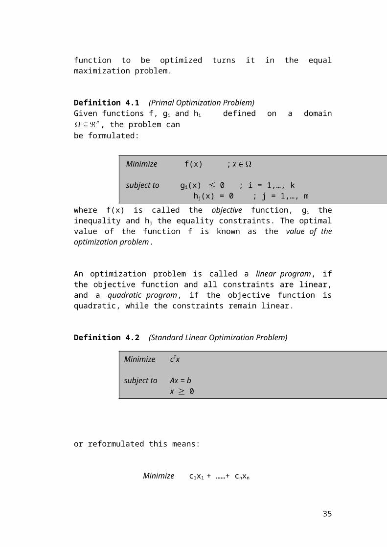
Definition 4.1 (Primal Optimization Problem)Given functions f, gi and hi defined on a domain , the problem can be formulated:

25

where f(x) is called the objective function, gi the inequality and hj the equal-ity constraints. The optimal value of the function f is known as the value of the optimization problem.

An optimization problem is called a linear program, if the objective function and all constraints are linear, and a quadratic program, if the objective function is quadratic, while the constraints remain linear.

Definition 4.2 (Standard Linear Optimization Problem)

or reformulated this means:

Minimize c1x1 + ……+ cnxn

subject to a11x1 + … + a1nxn = b1

……..an1x1 + … + annxn = bn

x 0

and another representation is:

It is possible to rewrite each common linear optimization problem in this standard form, even if the constraints are given as inequalities. For further readings on this topic one can refer to many good textbooks about optim-ization available. There are many ways to get the solution(s) of linear problems, e.g. Gaus-sian Reduction, Simplex with the Hessian Matrix, …., but we will not have such problems and therefore do not discuss these techniques here.

Minimize cTx

subject to Ax = b x 0

Minimize

subject to , mit i = 1…nx 0

26

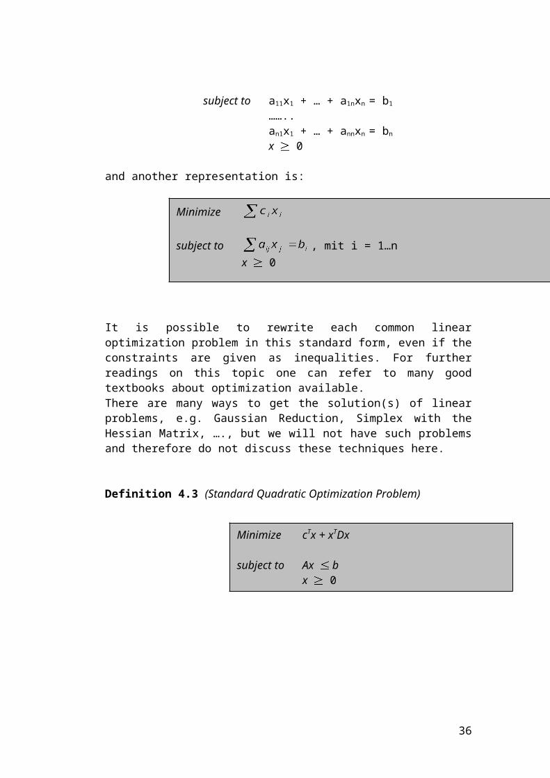
Definition 4.3 (Standard Quadratic Optimization Problem)

with Matrix D overall positive (semi-) definite, so the objective function is convex. Semi definite means, that for each x, xTDx 0 (in other words, D has non-negative eigenvalues). Non-convex functions and domains are not discussed here, because they will not play any role in the algorithms for Support Vector Machines. For further readings on nonlinear optimiza-tion, refer to [Jah96]. So in this problem you have variables x in the form x and , which does not lead to a linear system, where only the form x is found.

Definition 4.4 (Convex domains)

A subdomain D of the is convex, if for any two points x,y D the con-nection between them is also an element of D. Mathematically this means:

(1-h)x + hy Dfor all h [0,1], and x,y D

For example the is a convex domain. In figure 4.1 only the three upper domains are convex.

Minimize cTx + xTDx

subject to Ax b x 0

27

Figure 4.1: 3 convex and 2 non-convex domains

Definition 4.5 (Convex functions)

A function f is said to be convex in D , if the domain D is convex and for all x,y D and h [0,1] this applies:

f(hx + (1-h)y) hf(x) + (1-h)f(y)

In words this means, that the graph of the function always lies under the secant (or chord).

Figure 4.2: Convex and concave functions

Another criterion for convexity of twice differentiable functions is the posit-ive semi definiteness of the Hessian Matrix [Jah96].

28

The problem of minimizing a convex function on a convex domain (set) is known as a convex programming problem. The main advantage of such problems is the fact, that every local solution to the convex problem is also a global solution and that a global solution is always unique there. In non-linear, non-convex problems, the main problem are the local minimums. For example, algorithms implementing the Gradient-Descent (-Ascent) method to find a minimum (maximum) of the objective function cannot guarantee, that the found minimum is a global one, and so the solution would not be optimal.

In the rest of this diploma and in the support vector theory, the optimiza-tion problem can be restricted to the case of a convex quadratic function with linear constraints on the domain .

Figure 4.4: A local minimum of a nonlinear and non-convex function

4.2 LAGRANGIAN THEORY

The intention of the Lagrangian theory is to characterize the solution of an optimization problem initially, when there are no inequality constraints. Later the method was extended to the presence of inequality constraints, known as the Kuhn-Tucker theory.

To ease the understanding we first introduce the simplest case of optimiz-ation in absence of any constraints.

local minimum

29

Theorem 4.6 (Fermat)

A necessary condition for w* to be a minimum of f(w) f ,is that the first

derivation . This condition is also sufficient if f is a convex func-

tion.

Addition: A point x0=(x1…xn) realizing this condition is called a sta-tionary point of the function f: .

To use this on constrained problems, a function, known as the Lagrangian, is defined, that unites information about both the objective function and its’ constraints. Then the stationarity of this can be used to find solutions.

In appendix C you can find a graphical solution to such a problem in two variables and the calculated Lagrangian solution to the same problem. Also an example for the general case is formulated there.

Definition 4.7 (Lagrangian)

Given an optimization problem with objective function f(w) and the equality constraints h1(w) = c1, …. hn(w) = cn, the Lagrangian function is defined as

L(w,α) =

And as every equality can be transformed to hi(w) = 0 = , the Lag-rangian is

L(w, α) =

The coefficients αi are called the Lagrange multipliers.

Theorem 4.8 (Lagrange)

A necessary condition for a point w* to be a minimum (solution) of the objective function f(w) subject to hi(w) = 0 , i = 1…n, with f, hi is

30

(Derivation subject to w)

(Derivation subject to α )

These conditions are also sufficient in the case that L(w, α) is a convex function. This means the solution is a global optimum.

The conditions provide a linear system of n+m equations, with the last m the equality constraints (See appendix C for examples). By solving this system one obtains the solution.

Note: At the optimal point the constraints equal zero and so the value of the Lagrangian is equal to the objective function:

L(w, α) = f(w*)

As an interpretation of the Lagrange multiplier of the function , we assume it as a function of c and differentiate it with

respect to c:

But in the optimum L(w, α) = f(w*). So we can interpret that the Lagrange multiplier gives a hint on how the optimum is changing if the constant c of the constraint g(w) = c is changed.

Now to the most general case, where the optimization problem both con-tains equality and inequality constraints.

Definition 4.9 (Generalized Lagrangian Function)

The general optimization problem can be stated as

Minimize f(w)

subject to ; i = 1…k (inequalities); j = 1…m (equalities)

31

Then the generalized Lagrangian is defined as:

4.3 DUALITY

The introduction of dual variables is a powerful tool, because using this al-ternative - the dual - reformulation of an optimization problem often turns out to be easier to solve in contrast to its’ so called primal problem be-cause the handling of inequality constraints in the primal (which are often found) is very difficult. The dual problem to a primal problem is obtained by introducing the Lagrange multipliers, also called the dual variables. So the dual function does not depend on the primal variables anymore and solv-ing this problem is the same as solving the primal one. The new dual vari-ables are then considered to be the fundamental unknowns of the prob-lem. Duality is also a common procedure in linear optimization problems. For further readings look at [Mar00]. In general the primal minimization problem is then turned in the dual maximization one. So at the optimal solution point the primal and the dual function both meet with having an extreme there (convex functions would only have one global extreme).

Here we only look at the duality method important for Support Vector Ma-chines. To transform the primal problem in its’ dual one two steps are ne-cessary. First, the derivatives of the set up primal Lagrangian are set to zero with respect to the primal variables. Second, substitute the so gained relations back into the Lagrangian. This removes the dependency on the primal variables and corresponds to explicitly computing the new function

5

5 Inf = infimum The infimum of any subset of a linear order (linearly ordered set) is the

greatest lower bound of the subset. In particular, the infimum of any set of numbers is the

largest number in the set which is less than or equal to every other number in the set.

Rewritten this means:

32

For proof of this see [Nel00].

So overall the primal minimization problem of definition 4.1 can be trans-formed in the dual problem as:

Definition 4.10 (Lagrangian Dual Problem)

This strategy is a standard technique in the theory of Support Vector Ma-chines. As seen later, the dual representation allows us to work in high di-mensional spaces using so called Kernels without “falling prey to the curse of dimensionality”6. The Kuhn-Tucker complementary conditions, intro-duced in the following subchapter, lead to a significant reduction of the data involved in the training process. These conditions imply that only the active constraints have non-zero dual variables and therefore are neces-sary to determine the searched hyperplane. This observation will later lead to the term support vectors, as seen in chapter 5.

4.4 KUHN-TUCKER THEORY

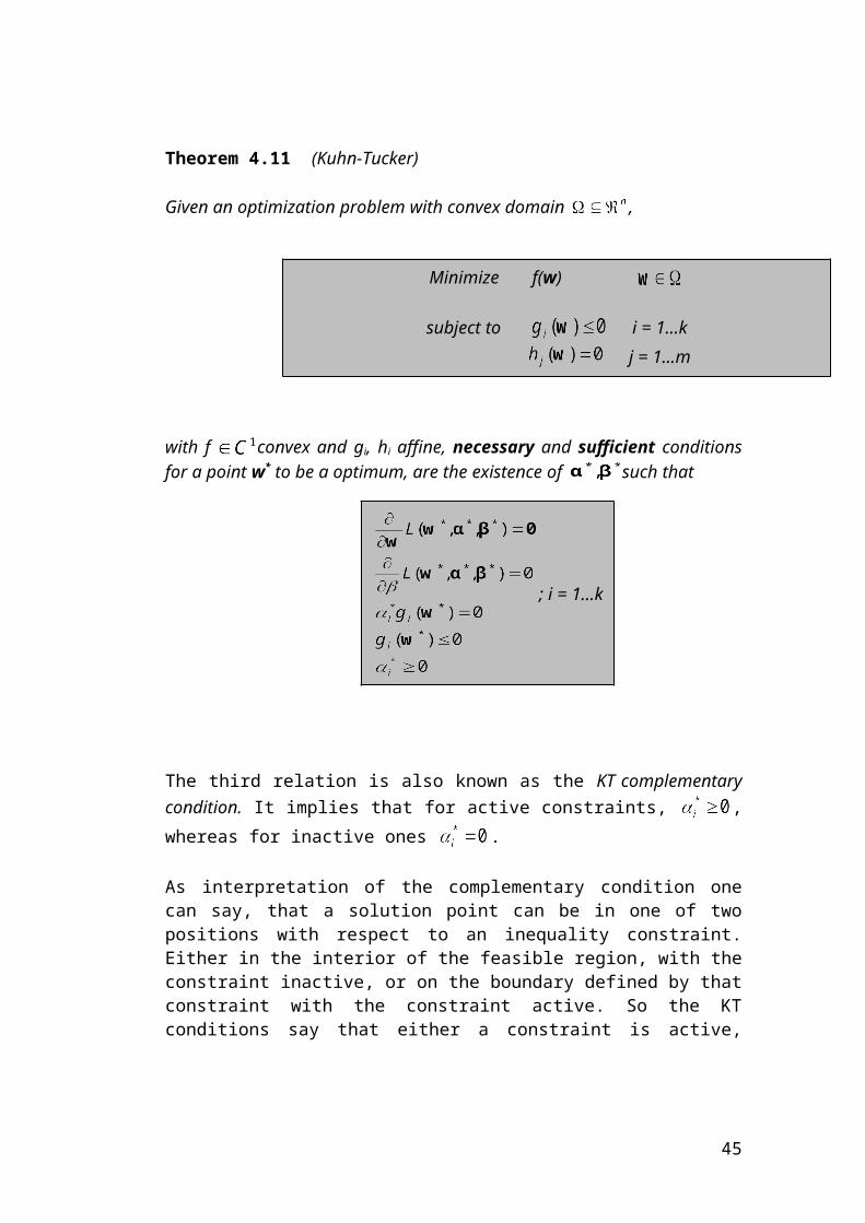
Theorem 4.11 (Kuhn-Tucker)

Given an optimization problem with convex domain ,

with f convex and gi, hi affine, necessary and sufficient conditions for a point w* to be a optimum, are the existence of such that

6 Explained in chapter 6

Minimize f(w)

subject to i = 1…kj = 1…m

; i = 1…k

Maximize

subject to

33

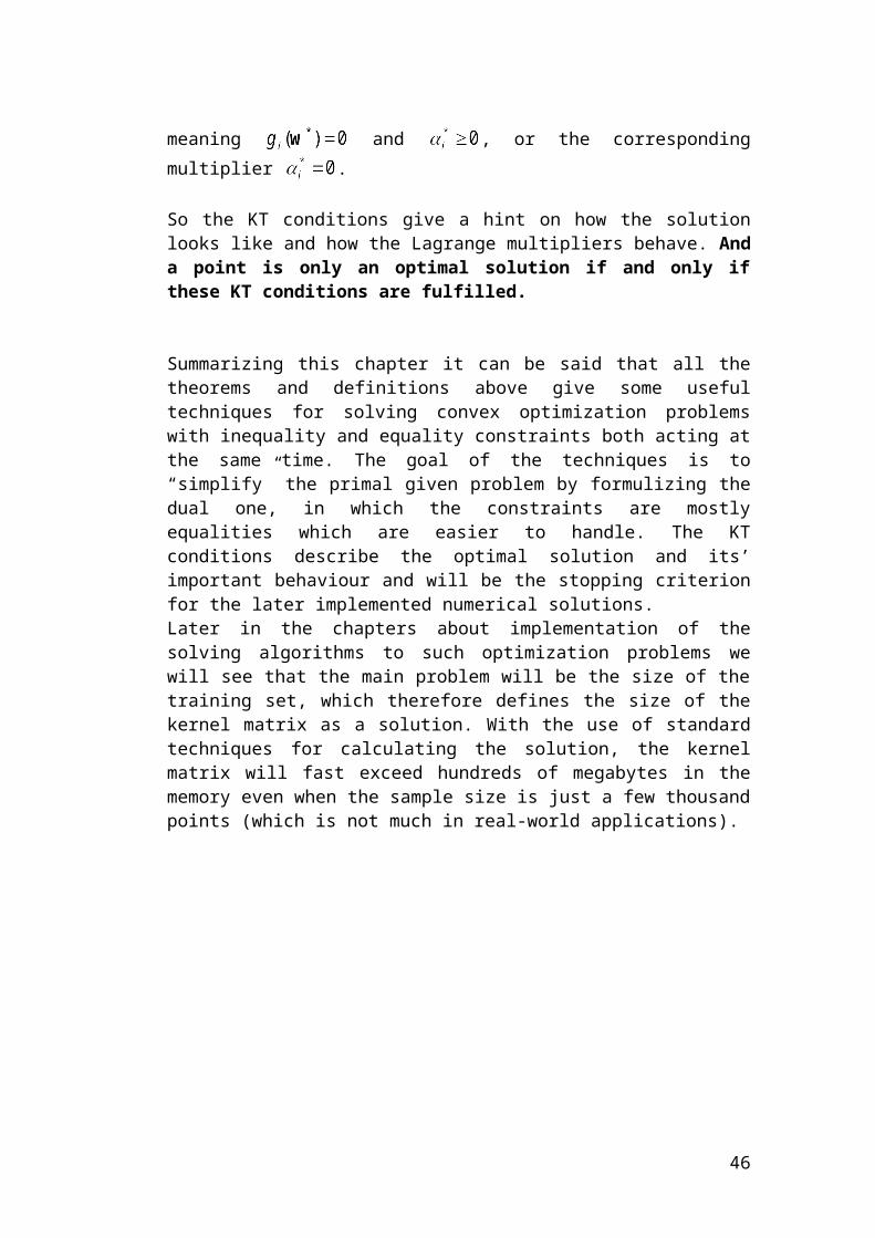
The third relation is also known as the KT complementary condition. It im-plies that for active constraints, , whereas for inactive ones .

As interpretation of the complementary condition one can say, that a solu-tion point can be in one of two positions with respect to an inequality con-straint. Either in the interior of the feasible region, with the constraint inact-ive, or on the boundary defined by that constraint with the constraint act-ive. So the KT conditions say that either a constraint is active, meaning

and , or the corresponding multiplier .

So the KT conditions give a hint on how the solution looks like and how the Lagrange multipliers behave. And a point is only an optimal solu-tion if and only if these KT conditions are fulfilled.

Summarizing this chapter it can be said that all the theorems and defini-tions above give some useful techniques for solving convex optimization problems with inequality and equality constraints both acting at the same time. The goal of the techniques is to “simplify” the primal given problem by formulizing the dual one, in which the constraints are mostly equalities which are easier to handle. The KT conditions describe the optimal solu-tion and its’ important behaviour and will be the stopping criterion for the later implemented numerical solutions. Later in the chapters about implementation of the solving algorithms to such optimization problems we will see that the main problem will be the size of the training set, which therefore defines the size of the kernel mat-rix as a solution. With the use of standard techniques for calculating the solution, the kernel matrix will fast exceed hundreds of megabytes in the memory even when the sample size is just a few thousand points (which is not much in real-world applications).

34

Part II

Support Vector Machines

35

Chapter 5

Linear Classification

5.1 Linear Classifiers on Linear Separable Data

As a first step in understanding and constructing Support Vector Machines we study the case of linear separable data, which is simply classified into two classes, the positive and the negative one, also known as binary clas-sification. To give a link to an example, important nowadays, imagine the classification problem of email into spam or not-spam. (A calculated ex-ample and examples on linear (non-)separable data can be found in Ap-pendix B.2)

This is frequently performed by using a real-valued function in the following way:The input x = (x1, … , xn)’ is assigned to the positive class, if , and otherwise to the negative one.

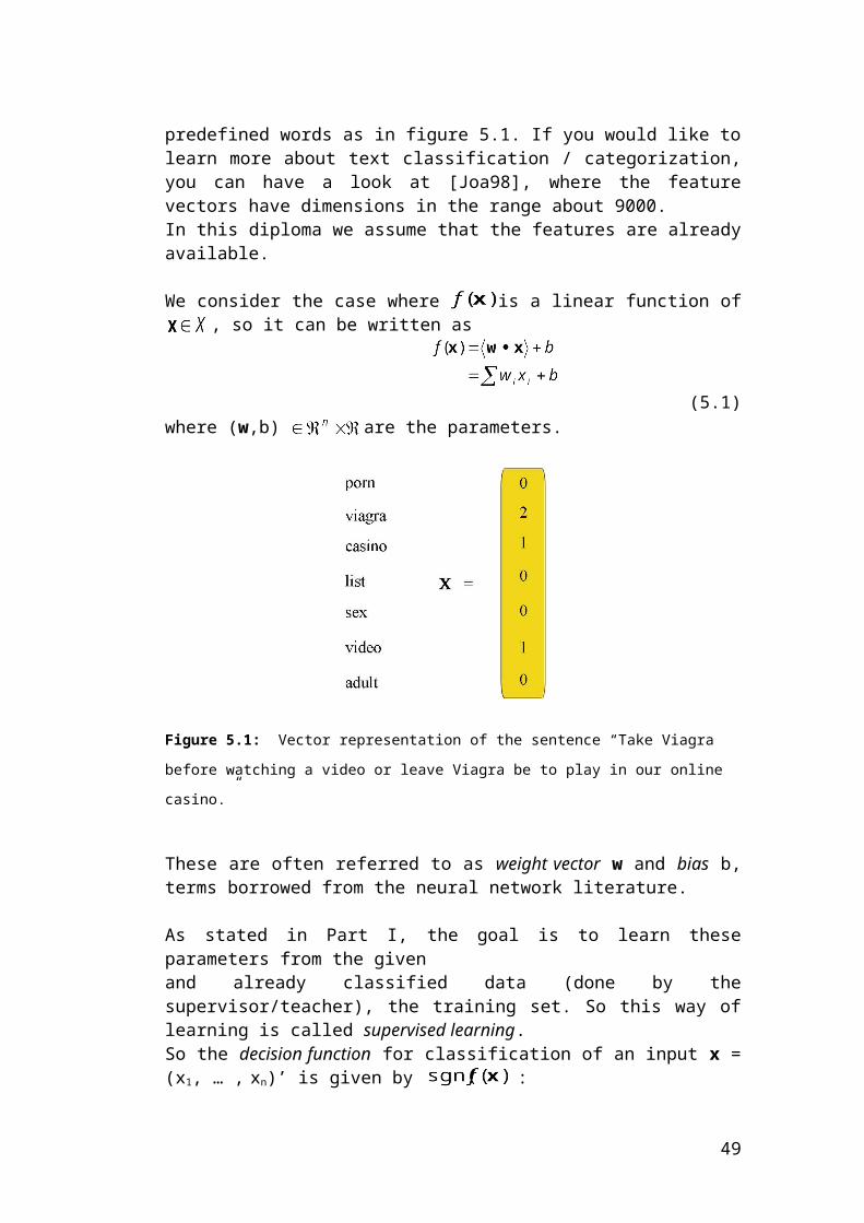
The vector x is build up by the relevant features which are used for classi-fication.In our spam example above we need to extract relevant features (certain words) from the text and build a feature vector for the corresponding docu-ment. Often such feature vectors consist of the counted numbers of pre-defined words as in figure 5.1. If you would like to learn more about text classification / categorization, you can have a look at [Joa98], where the feature vectors have dimensions in the range about 9000. In this diploma we assume that the features are already available.

We consider the case where is a linear function of , so it can be written as

(5.1)

where (w,b) are the parameters.

36

Figure 5.1: Vector representation of the sentence “Take Viagra before watching a video

or leave Viagra be to play in our online casino.”

These are often referred to as weight vector w and bias b, terms borrowed from the neural network literature.

As stated in Part I, the goal is to learn these parameters from the given and already classified data (done by the supervisor/teacher), the training set. So this way of learning is called supervised learning.So the decision function for classification of an input x = (x1, … , xn)’ is given by :

1, if (positive class)) =

-1, else (negative class)

Geometrically we can interpret this behaviour as follows (see figure 5.2):One can see that the input space X is split into two parts by the so called hyperplane defined by the equation .

This means, every input vector solving this equation is directly part of the hyperplane. A Hyperplane is an affine subspace7 of dimension n-1 which divides the space into two half spaces which correspond to the inputs of the two distinct classes.

7 A translation of a linear subspace of is called an affine subspace. For example, any

line or plane in is an affine subspace.

37

In the example of figure 5.2 n is 2, a two dimensional input space, so the hyperplane is simply a line here.The vector w therefore defines a direction perpendicular to the hyper-plane, so the direction of the plane is unique, while varying the value of b moves the hyperplane parallel to itself. Whereby negative values of b move the hyperplane, running through the origin, into the “positive direc-tion”.

In fact it is clearly to see that if one wants to represent all possible hyper-planes in the space the representation is only possible by involvingn + 1 free parameters, n ones given by w and one by b.

But the question that arises here is, which hyperplane to choose, because there are many possible ways in which it can separate the data. So we need a criterion for choosing ‘the best one’, the ‘optimal’ separating hyper-plane.

The goal behind supervised learning from examples for classification can be restricted to consideration of the two-class problem without loss of gen-erality. In this problem the goal is to separate the two classes by a func-tion, which is induced from available examples. The overall goal is to pro-duce a classifier (by finding parameters w and b) that will work well on un-seen examples, i.e. it generalizes well.

Figure 5.2: A separating hyperplane (w,b) for a two dimensional training set. The smaller

dotted lines represent the class of hyperplanes with same w and different values of b.

38

So if the distance between the separating hyperplane and the training points becomes too small, even test examples near to the given training points would be misclassified. Figure 5.3 illustrates this behaviour.

Therefore it seems that the classification of unseen data is much more successful in setting B than in setting A.This observation leads to the concept of the maximal margin hyperplanes, or the optimal separating hyperplane.

In appendix B.2 we have a closer look at an example with a ‘simple’ iterat-ive algorithm, separating points from two classes by means of a hyper-plane, the so called Perceptron. It is only applicable on linear separable data.There we also find some important issues, also stressed in the following chapters, which will have a large impact on the algorithm(s) used in the Support Vector Machines.

5.2 The Optimal Separating Hyperplane for Linear Separable Data

Definition 5.1 (Margin)

Figure 5.3: Which separation to choose ? Almost zero margin (A) or large margin (B) ?

39

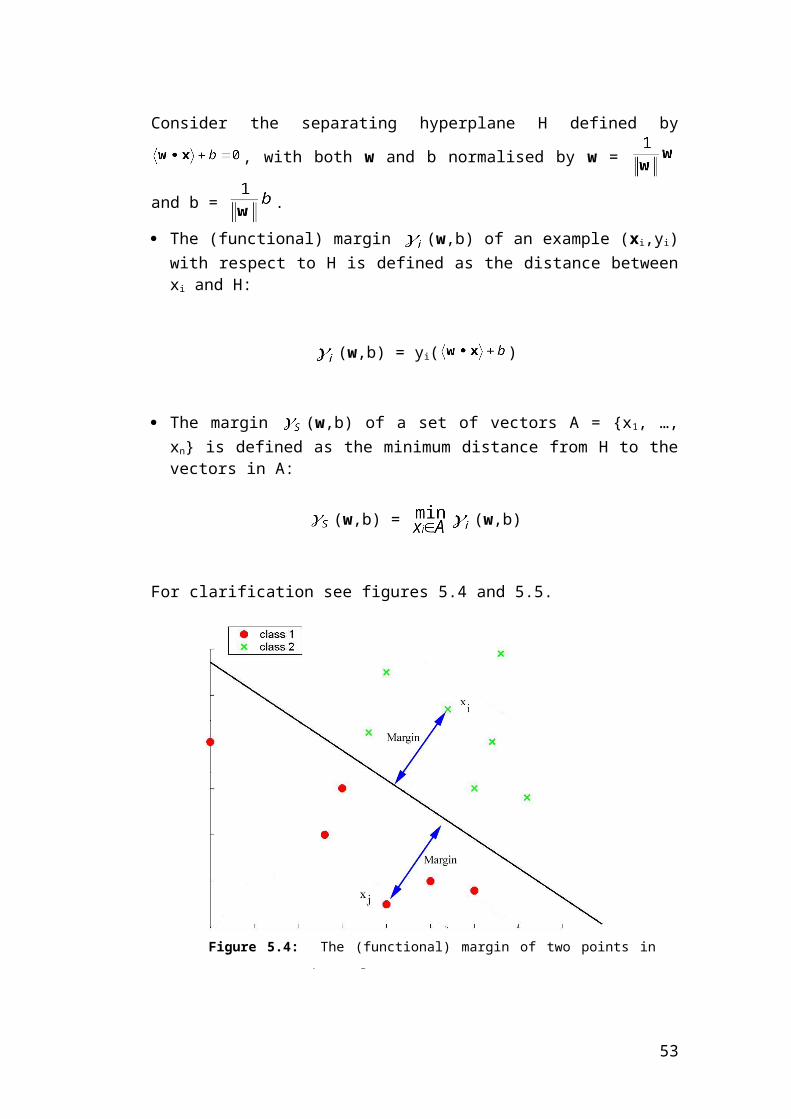
Consider the separating hyperplane H defined by , with both w

and b normalised by w = and b = .

The (functional) margin (w,b) of an example (xi,yi) with respect to H is defined as the distance between xi and H:

(w,b) = yi( )

The margin (w,b) of a set of vectors A = {x1, …, xn} is defined as the minimum distance from H to the vectors in A:

(w,b) = (w,b)

For clarification see figures 5.4 and 5.5.

In figure 5.5 we have introduced two new identifiers: d+ and d- : Let them be the shortest distance from the separating hyperplane H to the closest positive (negative) example (the smallest functional margin from each class). Then the geometric margin is defined as d+ + d- .

Figure 5.4: The (functional) margin of two points in respect to a hyperplane

40

So the goal is to maximize the margin

The training set is therefore said to be optimally separated by the hyper-plane, if it is separated without any error and the distance between the closest vectors to the hyperplane is maximal (maximal margin) [Vap98].

.

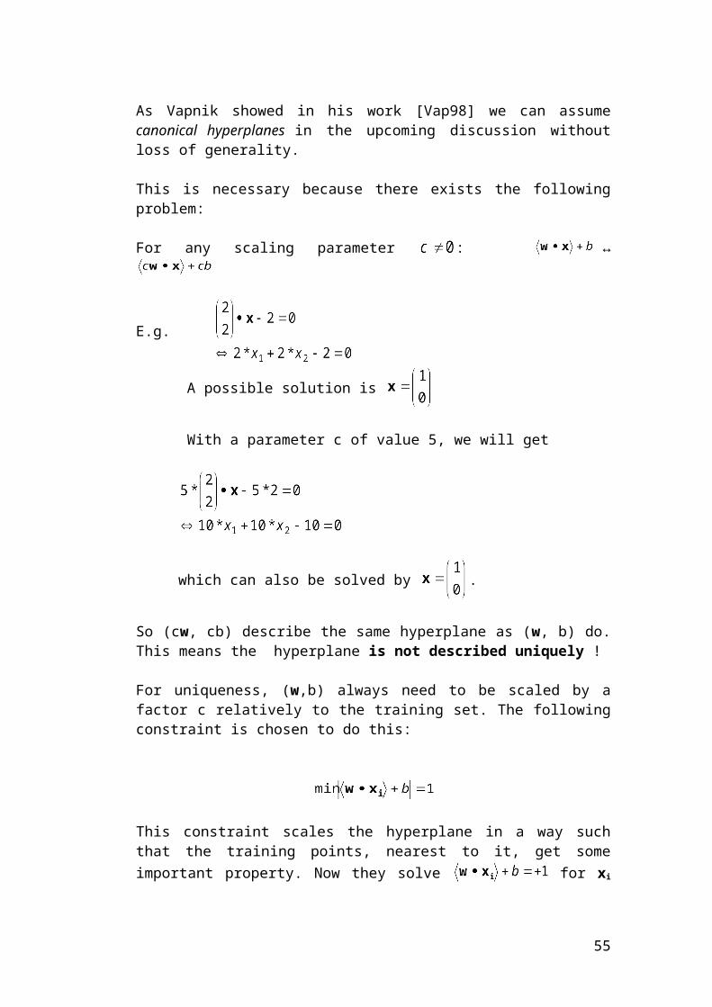
As Vapnik showed in his work [Vap98] we can assume canonical hyper-planes in the upcoming discussion without loss of generality.

This is necessary because there exists the following problem:

For any scaling parameter : ↔

E.g.

A possible solution is

With a parameter c of value 5, we will get

Figure 5.5: The (geometric) margin of a training set

41

which can also be solved by .

So (cw, cb) describe the same hyperplane as (w, b) do. This means the hyperplane is not described uniquely !

For uniqueness, (w,b) always need to be scaled by a factor c relatively to the training set. The following constraint is chosen to do this:

This constraint scales the hyperplane in a way such that the training points, nearest to it, get some important property. Now they solve

for xi of class yi = +1 and on the other side, for xi of class yi = -1.

A such scaled hyperplane is called a canonical hyperplane.Reformulated this means (implying correct classification):

; i = 1 … l (5.2)

This can be transformed into the following constraints:

for yi = +1 for yi = -1 (5.3)

Therefore it is clearly to see, that the hyperplanes H1 and H2 in figure 5.5 are solving and . They are called margin hyper-planes. Note that H1 and H2 are parallel, they have the same normal w (as H does too), and that no other training points fall between them in the margin ! They solve .

Definition 5.2 (Distance)

42

The Euclidian distance d(w,b; xi) of a point xi belonging to a class yi from the hyperplane (w,b) that is defined by is,

(5.4)

As stated above, training points (x1, +1) and (x2, -1) that are nearest to the so scaled hyperplane, respectively they lie on H1 and H2, have the dis-tance d+ = +1 and d- = -1 from it (see figure 5.5).

Or reformulated with equation 5.4 and constraints 5.3, this means:

and

and

and

So overall, as seen in figure 5.5, the geometric margin of a separating

canonical hyperplane is d+ + d-, and so .

As stated, the goal is to maximize this margin. That is achieved by minim-ising . The transformation to a quadratic function of the form

does not change the result but will ease later calculation.

This is because we now solve the problem with help of the Lagrangian method. There are two reasons for doing so. First the constraints of (5.2) will be replaced by constraints on the Lagrangian themselves, which will be much easier to handle (they are equalities then). Second the training data will only appear in the form of dot products between vectors, which will be a crucial concept later in generalizing the method on the nonlinear separable case and the use of kernels.

And so the problem is reformulated in a convex one, which is overall easier to handle by the Lagrangian method with its’ differentiations.

43

Minimize

subject to for yi = +1 for yi = -1

Summarizing we have the following optimization problem to solve:

Given a linearly separable training set S = ((x1,y1), …, (xl,yl))

(5.5)

The constraints are necessary to ensure uniqueness of the hyperplane, as mentioned above !

Note: , because

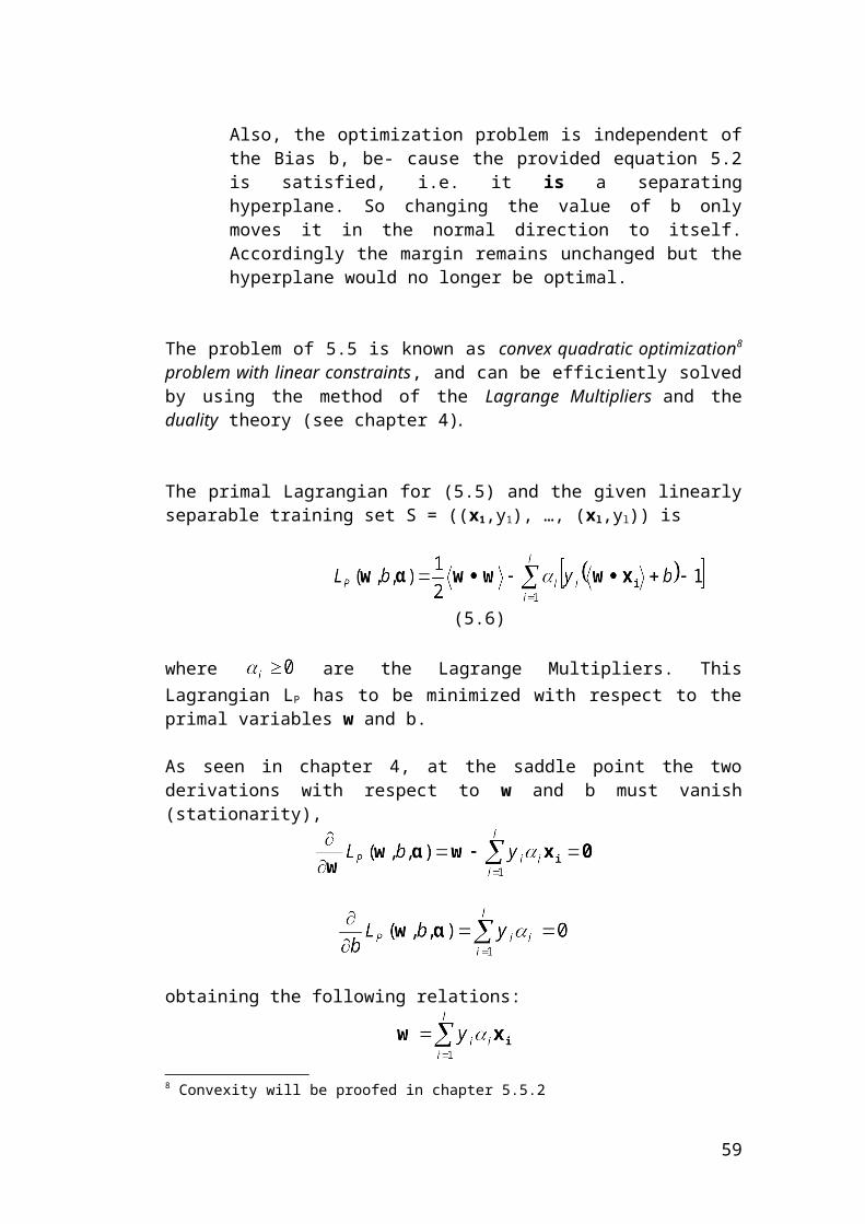
Also, the optimization problem is independent of the Bias b, be- cause the provided equation 5.2 is satisfied, i.e. it is a separating hyperplane. So changing the value of b only moves it in the nor-mal direction to itself. Accordingly the margin remains unchanged but the hyperplane would no longer be optimal.

The problem of 5.5 is known as convex quadratic optimization8 problem with linear constraints, and can be efficiently solved by using the method of the Lagrange Multipliers and the duality theory (see chapter 4).

The primal Lagrangian for (5.5) and the given linearly separable training set S = ((x1,y1), …, (xl,yl)) is

(5.6)

where are the Lagrange Multipliers. This Lagrangian LP has to be minimized with respect to the primal variables w and b.8 Convexity will be proofed in chapter 5.5.2

44

Maximize

subject to ; i = 1…l

As seen in chapter 4, at the saddle point the two derivations with respect to w and b must vanish (stationarity),

obtaining the following relations:

(5.7)

By substituting the relations (5.7) back into LP one arrives at the so called Wolfe Dual of the optimization problem (now only dependable on , no more w and b!):

(5.8)

So the dual problem for (5.6) can be formulated:Given a linearly separable training set S = ((x1,y1), …, (xl,yl))

(5.9)

Note: The matrix is known as the Gram Matrix G.

45

So the goal is to find parameters which solve this optimization problem. As a solution to construct the optimal separating hyperplane with maximal margin we obtain the optimal weight vector:

(5.10)

Remark: One can think that up to now, the problem will be able to be solved easily as the one in appendix C with the use of Lagrangian theory and the primal (dual) objective function. This could be right if having input vectors of small dimension, e.g. 2. But in the real-world case the number of variables will be over some thousand ones. Here solving the system with standard techniques will not be practicable in the case of time and memory usage of the corresponding vectors and matrices. But this issue will be discussed in the implementation chapter later.

5.2.1 Support Vectors

Stating the Kuhn-Tucker (KT) conditions for the primal problem LP above (5.6), as seen in chapter 4, we get

(5.11)

As mentioned, the optimization problem for SVMs is a convex one (a con-vex function, with constraints giving a convex feasible region). And for convex problems the KT conditions are necessary and sufficient for w*, b and to be a solution. Thus solving the primal/dual problem of the SVMs is equivalent to finding a solution to the KT conditions (for the primal)9 (see chapter 3, too).The fifth relation in (5.11) is known as the KT complementary condition.In the third chapter on optimization theory an intention was given on how it works. In the SVM´s problem it has a good graphical meaning. It states that for a given training point xi either the corresponding Lagrange Multi-plier equals zero or, if not zero, xi lies on one of the margin hyperplanes (see figure 5.4 and following text) H1 or H2:9 only they will be needed because the primal/dual problem is a equivalent one, so we will

maximize the dual (it is only dependable on !) and as a criterion take the KT conditions

of the primal.

46

On them are the training points xi with minimal distance to the optimal sep-arating hyperplane OSH (with maximal margin).The vectors lying on H1 or H2, implying are called Support Vectors (SV).

Definition 5.3 (Support Vectors)

A training point xi is called support vector, if its corresponding Lagrange multiplier .All other training points having either lie on one of the two margin hy-perplanes (equality of (5.2)) or on the side of H1 or H2 (inequality of (5.2)). A training point can be on one of the two margin hyperplanes, because the complementary condition in (5.11) only states that that all SVs are on the margin hyperplanes, but not that the SVs are the only ones on them. So there may be the case where both and .Then the point xi lies on one of the two margin hyperplanes without being a SV.

Therefore SVs are the only points involved in determining the optimal weight vector in equation (5.10).So the crucial concept here is that the optimal separating hyperplane is uniquely defined by the SVs of a training set. That means, repeating the training with all other points removed or moved around without crossing H1

or H2 lead to the same weight vector and therefore to the same optimal separating hyperplane. In other words, a compression has taken place. So for repeating the train-ing later, the same result can be achieved by only using the determined SVs.

47

Figure 5.6: The optimal separating hyperplane (OSH) with maximal margin is determ-

ined by the support vectors (SV, marked) lying on the margin hyperplanes H1 and H2.

Note that in the dual representation the value of b does not appear and so the optimal value b* has to be found making use of the primal constraints:

; i = 1 … l

So only the optimal value of w is explicitly determined by the training pro-cedure. This implies we have optimal values for . Therefore it is possible to pick any , a support vector, and so, with the substitution

in the above inequality the upper constraint becomes an

equality ( = 0 because a support vector always is part of a margin hyper-plane) and b can be computed.

Numerically it is safer to compute b for all i and take the mean value, or another approach as in the book [Nel00]:

(5.12)

48

Note: This approach to compute the bias has been shown to be problem-atic with regard to the implementation of the SMO algorithm, as showed by [Ker01]. This issue will be discussed in the implementation chapter later.

5.2.2 Classification of unseen data

After the hyperplanes’ parameters (w* and b*) have been learned with the training set we can classify unseen/unlabeled data points z. In the binary case (2 classes), discussed up to now, the found hyperplane divides the

into two regions. One where and the other one where . The idea behind the maximal margin classifier is to determ-

ine on which of the two sides the test pattern lies and to assign the label correspondingly with -1 or +1 (as all classifiers) and also to maximize the margin between the two sets. Hence the used decision function can be expressed with the optimal para-meters w* and b* and therefore by the found/used support vectors , their corresponding and b*.

So overall the decision function of the trained maximal margin classifier for some data point z can be formulated:

(5.13)

Whereby the last reformulation only sums over the elements, training point xi, corresponding label yi, associated and the bias b, which are associ-ated with a support vector (SV), because only they have and there-fore an impact on the sum.

All in all, the optimal separating hyperplane we get by solving the margin optimization problem is a very simple special case of a Support Vector Machine, because it computes directly on the input data. But it is a good starting point for understanding the forthcoming concepts. In the next chapters the concept will be generalized to nonlinear classifiers and there-fore the concept of Kernel mapping will be introduced. But first the adap-tion of the separating hyperplane on linearly non-separable data will be done.

49

5.3 The Optimal Separating Hyperplane for Linear Non-Separable Data

The algorithm above for the maximal margin classifier cannot be used in many real-world applications. In general noisy data will render linear sep-aration impossible but the hugest problem will still be the used features in practice leading to overlapping classes. The main problem with the max-imal margin classifier is the fact, that it allows no classification errors dur-ing training. Either the training is perfect without any errors or there is no solution at all. Hence it is intuitive that we need a way to relax the constraints of (5.3).But each violation of the constraints needs to be “punished” by a misclas-sification penalty, i.e. an increase in the primal objective function LP.This can be realized by introducing the so called positive slack variables (i = 1…l) in the constraints first and, as shown later, introduce an error weight C, too:

for yi = +1for yi = -1

As above, these two constraints can be rewritten into one:

;i= 1…l (5.14)

So the `s can be interpreted as a value that measures how much a point

fails to have a margin (distance to the OSH) of . So it indicates where

a point xi lies, compared to the separating hyperplane (see figure 5.7).

misclassification

is classified correctly, but lies inside the margin

is classified correctly and lies outside the margin or on the margin boundary

50

Minimize +

subject to ; i = 1…l

So a classification error is marked by the corresponding exceeding

unity. Therefore is an upper bound on the number of training errors.

Overall with the introduction of these slack variables the goal is to maxim-ize the margin and simultaneously minimize misclassifications.

To define a penalty on training errors the error weight C is introduced by

.

This parameter has to be chosen by the user. In practice, C is varied through a wide range of values and the optimal performance is assessed using a separate validation set or a technique called cross-validation for verifying performance just using the training set.

Figure 5.7: Values of slack variables: (1) misclassification if is larger than the mar-

gin ( ); (2) correct classification of xi lying in the margin with ; (3) correct

classification of xi outside the margin (or on it) with

So the optimization problem can be extended to

51

Maximize

subject to

i = 1…l

(5.15)

The problem is again a convex one for any positive integer k. This ap-proach is called the Soft Margin Generalization, while the original concept above is known as Hard Margin, because it allows no errors. The Soft Margin case is widely adapted to the values of k = 1 (1-Norm Soft Margin) and k = 2 (2-Norm Soft Margin).

5.3.1 1-Norm Soft Margin - or the Box Constraint

For k = 1, as above, the primal Lagrangian can be formulated as

with .

Note: As described in chapter 4, we need another parameter ß here, be-cause of the new inequality constraint .

As before, the corresponding dual representation is found by differentiat-ing LP with respect to w, and b:

By resubstituting these relations back into the primal we obtain the dual formulation LD:

Given a training set S = ((x1,y1), …, (xl,yl))

52

(5.16)

This problem is curiously identical to that for the maximal (hard) margin one in (5.9). The only difference is that together with enforces . So in the soft margin case the Lagrange multipliers are upper bounded by C. The Kuhn-Tucker complementary conditions for the primal above are:

;i = 1…l;i = 1…l

Another consequence of the KT conditions is that they imply that non-zero slack variables can only occur when and therefore . The cor-responding point xi has a distance less than 1/ from the hyperplane and therefore lies inside the margin.

This can be seen with the constraints (only shown for yi = +1, the other case is analogous):

for points on the margin hyperplane.

And therefore points xi with non-zero slack variables have a distance less than 1/ .

Points for which then lie exactly at the target distance of 1/ and therefore on one of the margin hyperplanes ( ). This also shows that the hard margin hyperplane can be attained in the soft margin case by setting C to infinity ( ).The fact that the Lagrange multipliers are upper bounded by the value of C gives the name to this technique: box constraint. Because the vector is constrained to lie inside the box with side length C in the positive orthant ( ). This approach is also known under SVM with linear loss function.

5.3.2 2-Norm Soft Margin - or Weighting the Diagonal -

53

Maximize

subject to

;i = 1…l

This is the case for k = 2. But before stating the primal Lagrangian and for ease of the upcoming calculation, note that for the first constraint of (5.15) still holds if . Hence we still obtain the optimal solution when the positivity constraint on is removed. So this leads to the following primal Lagrangian:

with the Lagrange multipliers again. As before the corresponding dual is found by differentiating with respect to w, and b, imposing stationarity (i.e. setting to zero):

and again resubstituting the relations back into the primal to obtain the dual formulation LD:

Using the equation

where is the Kronecker Delta, which is defined to be 1 if i = j and 0 oth-erwise. So on the right side of above equation inserting changes noth-ing at the result because is either +1 or -1 and is the same as writing , and so we simply multiply extra by 1, but can simplify LD to get the final problem to be solved:

Given a training set S = ((x1,y1), …, (xl,yl))

54

(5.17)

The complementary KT conditions for the primal problem above are

;i = 1…l

This whole problem can be solved with the same methods used for the maximal margin classifier. The only difference is the addition of 1/C to the diagonal of the Gram matrix G = . Only on the diagonal, because of the Kronecker Delta. This approach is also known under SVM with quad-ratic loss function.

Summarizing this subchapter it can be said that the soft margin optimiza-tion is a compromise between little empirical risk and maximal margin. For an example look at figure 5.8. The value of C can be interpreted as repres-enting the trade-off between minimizing the training set error and maximiz-ing the margin. So all in all, by using C as an upper bound on the Lag-range multipliers, the role of “outliers” is reduced by preventing a point from having too large Lagrange multipliers.

(a)

55

(b)

(c)

Figure 5.8: Decision boundaries arising when using a Gaussian kernel with fixed value

of in the three different machines: (a) the maximal margin SVM, (b) the 1-norm soft

margin SVM and (c) the 2-norm soft margin SVM. The data are an artificially created two

dimensional set. The blue dots being positive examples and the red ones negative ex-

amples.

56

5.4 The Duality of Linear Machines

This section is intended to stress the fact that was used and remarked several times before. The linear machines introduced above can be formu-lated in a dual description. This reformulation will turn out to be crucial in the construction of the more powerful generalized Support Vector Ma-chines below.

But what does ‘duality of classifiers’ mean ?As seen in the former chapter the normal vector w can be represented as a linear combination of the training points:

with S = ((x1,y1), …, (xl,yl)) the given training set already classified by the supervisor. The were introduced in the used Lagrange way to find a solution to the margin maximization problem. They were called the dual variables of the problem and therefore the fundamental unknowns. On the way to the solution we then obtain

and the reformulated decision function for unseen data z of (5.13):

The crucial observation here is that the training and test points never act through their individual attributes. These points only appear as entries in the Gram Matrix G = in the training phase and later in the test phase they only appear in an inner product with the training points .

5.5 Vector/Matrix Representation of the Optimization Problem and Summary

57

Maximize

subject to

i = 1…l

5.5.1 Vector/Matrix Representation

To give a first impression on how the above problems can be solved using a computer, the problem(s) will be formulated in the equivalent notation with vectors and matrices. This notation is more practical, understandable and are used in many implementations.

As described above, the convex quadratic optimization problem which arises for hard ( ), 1-norm ( ) and 2-norm (change the Gram mat-rix by means of adding 1/C to the diagonal) margin is the following:

This problem can be expressed as:

(5.18)

where e is the vector of all ones, C > 0 the upper bound, Q is a l by l posit-ive semidefinite10 matrix, .

And with a correct training set S = ((x1,y1), …, (xl,yl)) with the length of l (5.18) would look like:

10 Semidefinite: For each , (Q has non-negative eigenvalues). Also see next

page for explanation

Maximize

subject to i = 1…l

58

Maximize

subject to

i = 1…l

5.5.2 Summary

As seen in chapter 4 quadratic problems with a so called positive (semi-) definite matrix are convex functions. This allows the crucial concepts of solutions to convex functions to be adapted (see chapter 4: convex, KT). In former chapters the convexity of the objective function has been as-sumed without proof.

So let M be any (possibly non-square) matrix and set A = MTM. Then A is a positive semi-definite matrix since we can write

, (5.19)

for any vector x. If we take M to be the matrix whose columns are the vec-tors , i = 1…l, then A is the Gram Matrix ( ) of the set S = (x1, …, xl), showing that Gram Matrices are always positive semi-definite.

And therefore the above matrix Q also is positive semi-definite.

Summarized, the problem to be solved up to now can be stated as

(5.20)

with the particularly simple primal KT conditions as criterions for a solution to the 1-norm optimization problem:

59

(5.21)

Notice that the slack variables do not need to be computed for this case, because as seen in chapter 5.3.1, they will only be non-zero if and

. And so recall the primal of this chapter, stated as

Then

set , , so the third sum is zero and from the second sum we get

which is equivalent to and so it will be deleted and no slack

variable is there anymore.

For the maximal margin case the conditions will be:

(5.22)

And last but not least for the 2-norm case:

(5.23)

The last condition is reformulated by means of implicitly defining with

help of the primal KT condition of chapter 5.3.2 and

therefore . And with the complementary KT condition

the third condition above is gained.

As seen in the soft margin chapters, points for which the second equation holds are Support Vectors on one of the margin hyperplanes and for which the third one holds are inside the margin, therefore called “margin-errors”.

These KT conditions will be used later and proof to be important when im-plementing algorithms for computational numerical solving the problem of (5.20). Because a point is an optimum of (5.20), if and only if the KT con-

60

ditions are fulfilled and is positive semi-definite. The second requirement is proven above.

And after the training process (the solving of the quadratic optimization problem and as a solution getting the vector and therefore bias b), the classification of unseen data z is performed by

(5.23)

where the are the training points with their corresponding greater than zero and upper bounded by C and therefore support vectors.

As one can think now the question arising here is why always classify new data by the use of the and why not simply saving the resulting weight vector w ? Sure up to now it will be possible to do that and so no further need of having to store the training points and their labels . But as seen above there will be very few support vectors normally and only them and their corresponding and are necessary to reconstruct w. But the main reason will be given in chapter 5, where we will see that we must use the and not simply store w.

To give a short link to the implementation issue discussed later, it can be said that in most cases the 1-norm is used, because in real-world applica-tions you normally will not have noise-free, linear separable data, and therefore the maximal margin approach will not lead to satisfactory results. But the main problem is still the selection of the used feature data in prac-tice. The 2-norm is used in fewer cases, because it is not easy to integrate in the SMO algorithm, discussed in the implementation chapter.

61

Chapter 6

Nonlinear Classifiers

The last chapter showed how the linear classifiers can easily be computed by means of standard optimization techniques. But linear learning ma-chines are restricted because of their limited computational power as high-lighted in the 1960’s by Minsky and Papert. Summarized it can be stated that real-world applications require more expressive hypothesis spaces than linear functions. Or in other words, the target concept may be too complex to be expressed as a “simple” linear combination of the given at-tributes (That’s what linear machines do), equivalent to: the decision func-tion is not a linear function of the data. This problem can be overcome by the use of the so called kernel technique. The general idea is to map the input data nonlinearly to a (nearly always) higher dimensional space and then separate it their by linear classifiers. Therefore this will result in a nonlinear classifier in input space (see figure 6.1). Another solution to this problem has been proposed in the neural network theory: Multiple layers of thresholded linear functions which led to the development of multi-layer neural networks.

Figure 6.1: Simpler classification task by a feature map(Φ). 2-dimensional Input space

on the left, 2-dimensional feature space on the right, where we are able to separate by a

linear classifier which leads to the nonlinear classifier in input space.

62

6.1 Explicit Mappings

Now the representation of training examples will be changed by mapping the data to a (possibly infinite dimensional) Hilbert space11 F. Usually the space F will have a much higher dimension than the input space X. The mapping is applied to each labelled example before training and then the optimal separating hyperplane is constructed in the space F.

(6.1)

This is equivalent to mapping the whole input space X into F.

The components of are called features, while the original quantities are sometimes referred to as the attributes. F is called the feature space. The task of choosing the most suitable representation of the data is known as feature selection. This can be a very difficult task. There are different approaches existing to feature selection. Frequently one seeks to identify the smallest set of features that still conveys the essential information con-tained in the original attributes. This is known as dimensionality reduction,

(6.2)

and can be very beneficial as both computational and generalization per-formance can degrade as the number of features grows, a phenomenon known as the curse of dimensionality. The difficulties one is facing with high dimensional feature spaces is, that since the larger the set of (prob-ably redundant) features is, the more likely it is that the function to be learned could be represented using a standardised learning machine.Another approach to feature selection is the detection of irrelevant fea-tures and their elimination. As an example consider the gravitation law, which only uses information about the masses and the position of two bod-ies. So an irrelevant feature would be the colour or the temperature of the two bodies.

So as a last word to say on feature selection, it should be considered well as a part of the learning process. But it is also naturally a somewhat arbit-rary step, which needs some prior knowledge on the underlying target function. Therefore recent research has been done on the techniques for feature reduction. However in the rest of the diploma we do not talk about

11 Is a vector space with some more restrictions. A space H is separable if there exist a

countable subset , such that every element of H is the limit of a sequence of ele-

ments of . A Hilbert space is a complete separable inner product space. Finite dimen-

sional vector spaces like are Hilbert spaces. This space will be described in detail a

little further in this chapter and for further readings see [Nel00].

63

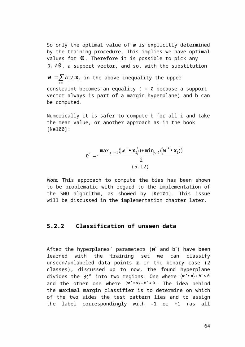
the feature selection techniques because as Christianini and Shawe-Taylor proofed in their book [Nel00] we can afford to use infinite dimen-sional feature spaces and avoid computational problems by the means of the implicit mapping, described in the next chapter. So the “curse of di-mensionality” can be said to be irrelevant by implicitly mapping the data, also known as the Kernel Trick.

Before illustrating the mapping with an example, first notice that the only way in which data appears in the training problem is in the form of dot products . Now suppose this data is first mapped to some other (possible infinite dimensional) space F, using the mapping of (6.1):

Then of course, as seen in (6.1) and (6.2) the training algorithm would only depend on the data through dot products in F, i.e. on functions of the form

(all other variables are scalars). Second there is no vector

mapping to w via , but we can write w in the form and

the whole hypothesis (decision) functions will be of the type

,

or reformulated

.

So a support vector machine is constructed which “lives” in the new higher dimensional space F but all the considerations of the former chapters will still hold, since we are still doing a linear separation, but in different space.

But now a simple example with explicit mapping.

Consider a given training set S = ((x1,y1), …, (xl,yl)) of points in with class labels +1 and -1: . Trivially these three points are not separable by a hyperplane, here a point12, in (see figure6.2). So first the data is nonlinearly mapped to the by applying

12 Input dimension is 1, therefore the hyperplane is of the dimension 1 – 1 = 0, and dim(0)

is defined as 1.

64

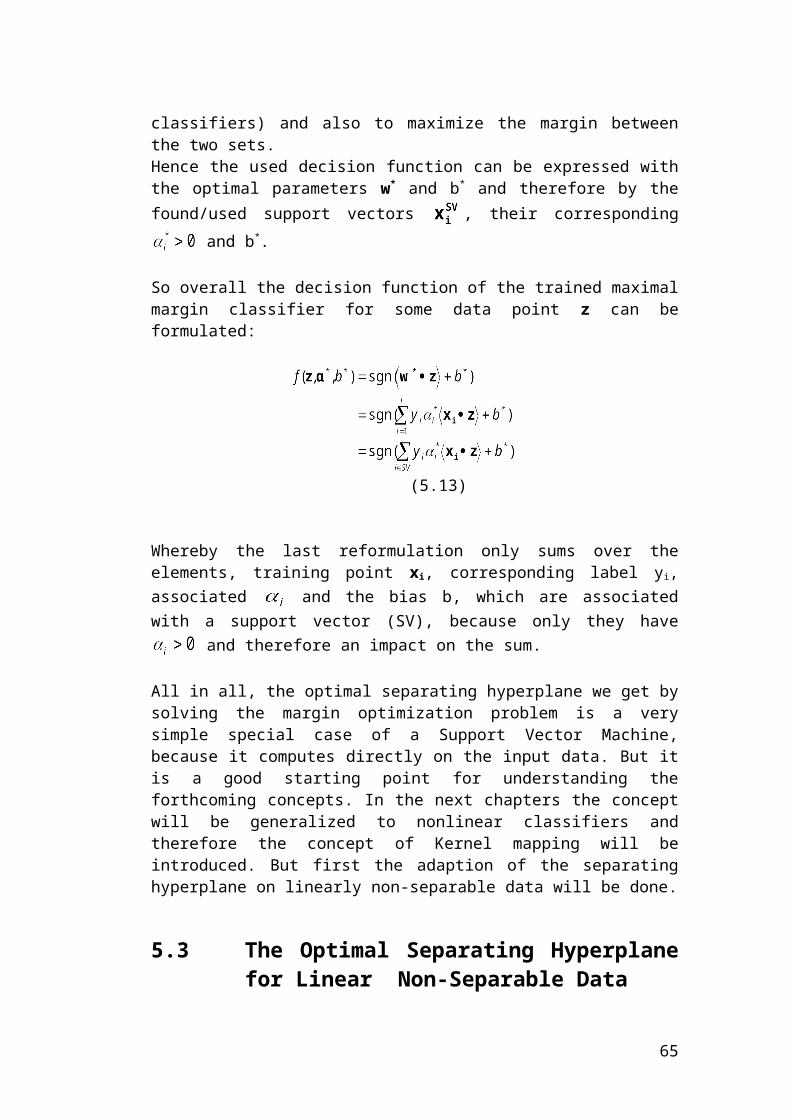
Figure 6.2: A non-separable example in the input space . The hyperplane would be a

single point but it cannot separate the data points.

This Step results in a training set consisting of the vectors

with the corresponding labels (+1, -1, +1). As illustrated

in figure 6.3 the solution in the new space can be easily seen geometri-

cally in the -plane (see figure 6.4). It is therefore , which is al-

most normalized yet meaning it has a length of 1, and the bias b becomes b = -0.5 (negative b means moving the hyperplane running through the ori-gin in the “positive direction”). So it can be seen that the learning task can be easily solved in the by linear separation. But how does the decision function look like in the original space , where we need it ?

Remember that w can be written in the form .

65

Figure 6.3: Creation of a separating hyperplane, i.e. a plane in the new space .

Figure 6.4: Looking at the -plane, the solution to w and b can be easily given by

geometric interpretation of the picture.

66

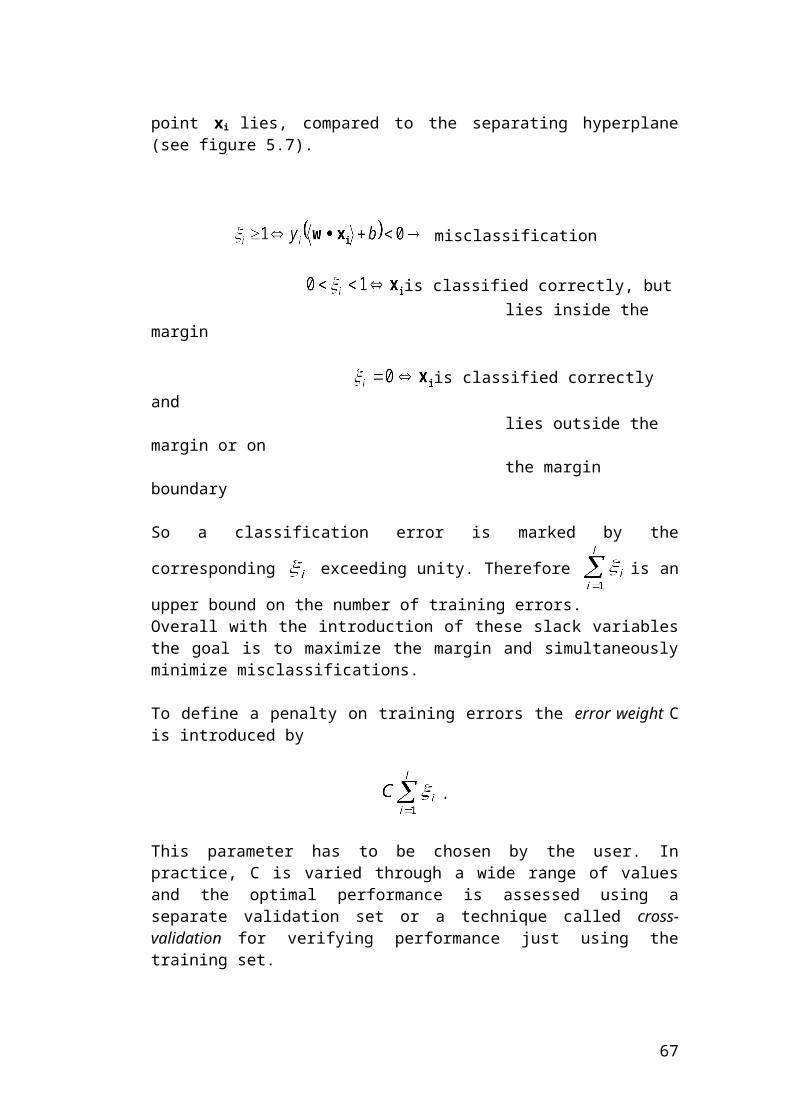
And in our particular example it can be written as :

And worked out:

The solving vector is then .

With the equation (6.3)

The hyperplane in then becomes with the original training points in : ; i = 1…3

This leads to the nonlinear hyperplane in consisting of two points: and .

As seen in equation (6.3), the inner product in the feature space has a equivalent function in the input space. Now we introduce an abbreviation for the dot product in feature space:

(6.4)

Clearly, that if the feature space is very high-dimensional, or even infinite dimensional, the right-hand side of (6.4) will be very expensive to com-pute. The observation in (6.3) together with the problem described above motivates to search for ways to evaluate inner products in feature space without making direct use of the feature space nor the mapping . This approach leads to the terms Kernel and Kernel Trick.

67

6.2 Implicit Mappings and the Kernel Trick

Definition 6.1 (Kernel Function)

Given a mapping from input space X to an (inner product) feature space13 F, we call the function a kernel function if for all

. (6.5)

The kernel function then behaves like an inner product in feature space but can be evaluated as a function in input space.

For example take the polynomial kernel . Now assume we have got d = 2 and (original input space), so we get:

13 Inner product space: A vector space X is called a inner product space if there exists a

bilinear map (linear in each argument) that for each two elements x, y X gives a real

number denoted by satisfying the following properties:

, and

e.g.: are fixed positive numbers.

Then the following defines a valid inner product:

where A is the n x n diagonal (only diagonal non-zero) matrix with non-zero

entries .

68

(6.6)

So the data is mapped to the .

But the second line can be left out by implicitly calculating with the vectors in input space:

what is the same as in the above calculation first mapping the input vec-tors to the feature space and then calculating the dot product:

.

So by implicitly mapping the input vectors to the feature space we are able to calculate the dot product there without even knowing the underlying mapping !

Summarized it can be stated that by implicitly performing such a non-linear mapping to a higher dimensional space, it can be done without increasing the number of parameters, because the kernel function computes the in-ner product in feature space only by use of the two inputs in input space.

To generalize here, a polynomial kernel with and at-tributes in input space of dimension n maps the data to a feature space of

dimension 14. In the example of (6.6) this means with n = 2 and d

= 2:

14 , called the binomial coefficient

69

And as can be seen above the data is really mapped from the to the .

In figure 6.5 the whole “new” procedure for classification of an unknown point z is shown, after training of the kernel-based SVM and therefore hav-ing the optimal weight vector w (defined by the ’s, the corresponding training points and their labels ) and the bias b.

Figure 6.5: The whole procedure for classification of a test vector z (in this example the test and training vectors are simple digits).

To stress the important facts, summarizing it can be said that in contrast to the example in chapter 6.1 the chain of arguments is inverted in that way, that there we started by explicitly defining a mapping before applying the learning algorithm. But now the starting point is choosing a kernel function K which implicitly defines the mapping and therefore avoiding the fea-ture space in the computation of inner products as well in the whole design of the learning machine itself. As seen above both the learning and test step only depend on the value of inner products in feature space. Hence, as shown, they can be formulated in terms of kernel functions. So once such a kernel function has been chosen, the decision function for unseen data z, (5.23), becomes:

70

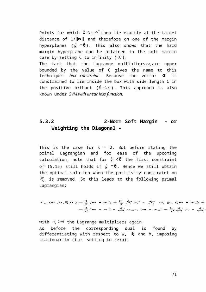
(6.7)

And as said before as a consequence we do not need to know the under-lying feature map to be able to solve the learning task in feature space !

Remark: As remarked in chapter 5, the consequence of using kernels is that now the direct storing of the resulting weight vector w is not practic-able, because as seen in (6.7) above, then we have to know the mapping and cannot use the advantage arising by the usage of kernels.

But which functions can be chosen as kernels ?

6.2.1 Requirements for Kernels - Mercer’s Condition -

As a first requirement for a function to be chosen as a kernel, definition 6.5 gives two conditions because the mapping has to be to an inner product feature space. So it can be easily seen that K has to be a symmetric func-tion:

(6.8)

And another condition for an inner product space is the Schwarz Inequal-ity:

(6.9)

However these conditions are not sufficient to guarantee the existence of a feature space. Here Mercer’s Theorem gives sufficient conditions (Vapnik 1995; Courant and Hilbert 1953).

The following formulation of Mercer’s Theorem is given without proof, as it is stated in the paper of [Bur98].

Theorem 6.2 (Mercer’s Theorem)

71

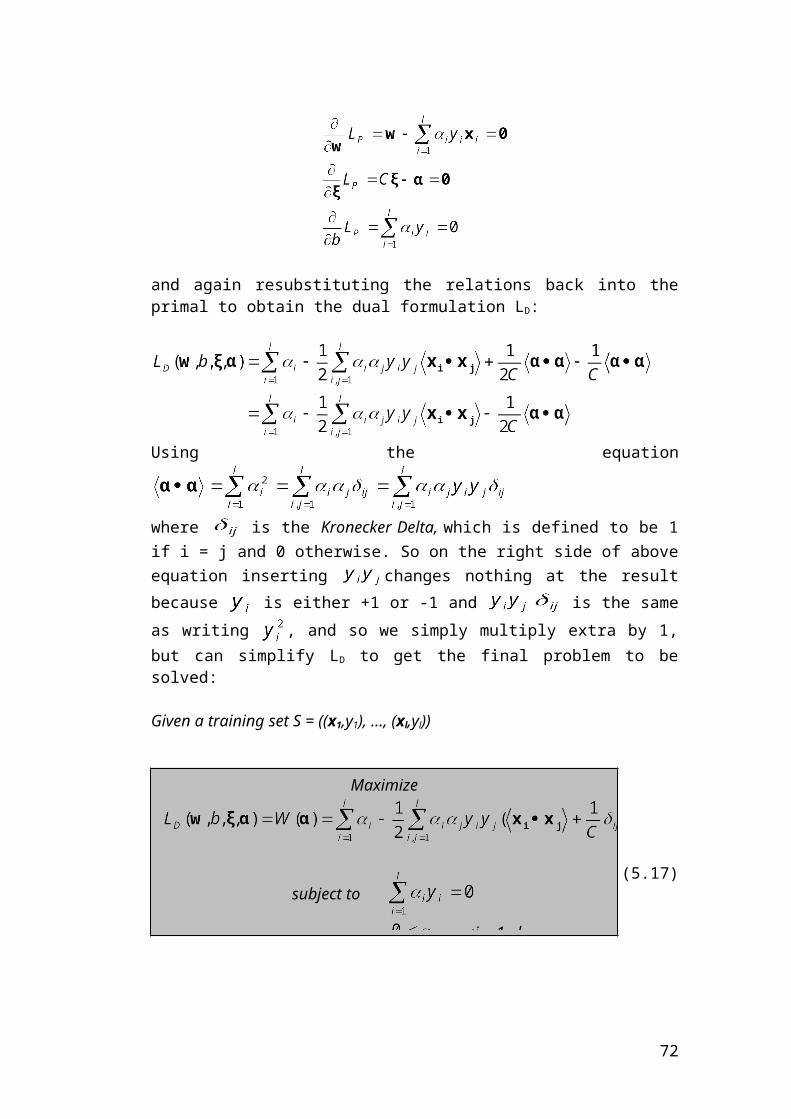
There exist a mapping and an expansion if and only if, for any g(x) such that

(is finite) (6.10)

then

(6.11)

Note: (6.10) has to hold for every g satisfying (6.10). This theorem is also sufficient for the infinite case.

Another simplified condition for K to be a kernel in the finite case can be seen from (6.8), (6.9) and when describing K with its’ eigenvectors and ei-genvalues (The proof is given in [Nel00]).

Proposition 6.3 Let X be a finite input space with K(x, z) a symmetric function on X. Then K(x, z) is a kernel function if and only if the matrix K is positive semi-definite.

Therefore Mercer’s Theorem is an extension of this proposition based on the study of integral operator theory.

6.2.2 Making Kernels from Kernels

Theorem 6.2 is the basic tool for verifying that a function is a kernel. The remarked proposition 6.3 gives the requirement for a finite set of points. Now this criterion for a finite set is applied to confirm that a number of new kernels can be created. The next proposition of Christianini and John Shawe-Taylor [Nel00] allows creating more complicated kernels from simple building blocks:

Proposition 6.4 Let and be kernels over , , f() a real-valued function on X,

72

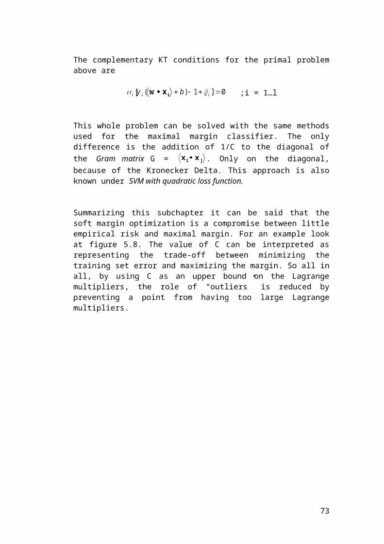
with a kernel over ,p() a polynomial with positive coefficients and B a symmetric positive semi-definite n x n matrix. Then the following functions are kernels, too:

K(x, z) = (x, z) + (x, z)

K(x, z) = a (x, z)

K(x, z) = (x, z) (x, z)

K(x, z) = f(x)f(z)

(6.12) K(x, z) = (

K(x, z) =

K(x, z) = p( (x, z))

K(x, z) = exp( (x, z))

6.2.3 Some well-known Kernels

The selection of a kernel function is an important problem in applications although there is no theory to tell which kernel when to use. Moreover it can be very difficult to check that some particular kernel satisfies Mercer’s conditions, since they must hold for every g satisfying (6.10). In the follow-ing some well known and widely used kernels are presented. Selection of the kernel, perhaps from among the presented ones, is usu-ally based on experience and knowledge about the classification problem at hand, and also theoretical considerations. The problem of choosing a kernel and its’ parameters on the basis of theoretical considerations will be discussed in chapter 7. Each kernel will be explained below.Polynomial K(x, z) = (6.13)

73

Sigmoid K(x, z) = (6.14)

Radial Basis Function

- Gaussian Kernel - K(x, z) = (6.15)

6.2.3.1 Polynomial Kernel

Here p gives the degree of the polynomial and c is some non-negative constant, usually c = 1. Usage of another generalized inner-product in-stead of the standard inner product above was proposed in many other works on SVMs because the Hessian matrix then becoming zero in nu-merical calculations (this means, no solution for the optimization problem). Then the Kernel will become:

K(x, z) =

Where the vector is such chosen that the function satisfies Mercer’s con-dition.

Figure 6.6: A polynomial kernel of degree 2 used for the classification of the non-separ-

able XOR-data set (in input space, by a linear classifier). Each colour represents one

class and the dashed lines mark the margins. The level of shading indicates the func-

tional margin, or in other words: The darker the shading of one colour representing a spe-

74

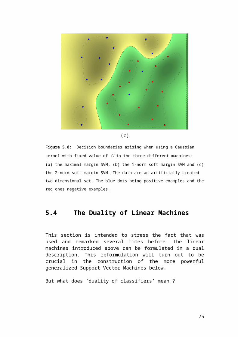
cific class, the more confident the classifier is that this point in that region belongs to that

class.

6.2.3.2 Sigmoid-function

The Sigmoid kernel stated above usually satisfies Mercer’s condition only for certain values of the parameters and . This was noticed experi-mentally by Vapnik. Currently there are no theoretical results on the para-meter values that satisfy Mercer’s conditions. As stated in [Pan01] the us-age of the sigmoid kernel with the SVM can be regarded as a two-layer neural network. In such networks the input vector z is mapped by the first layer into the vector F = ( ), where , i= 1…N and the dimension of F is called the number of the Hidden Units. In the second layer the sign of the weighted sum of the elements of F is calcu-lated by using weights . Figure 6.7 illustrates that.The main difference to notice between SVMs and two-layer neural net-works is the different optimization criterion: In the SVM case the goal is to find the optimal separating hyperplane which maximizes the margin (in the feature space), while in a two-layer neural network the criterion is usually to minimize the empirical risk associated with some loss function, typically the mean squared error.

z

1F

2F

NF

.

.

.

y

1

2

N

+1 / -1

Figure 6.7: A 2-layer neural network with N hidden units. Output of the first layer are of the form , i = 1…N. While the output of the whole network then

becomes .

75

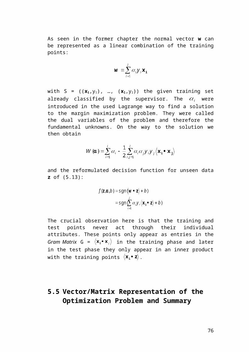
Another important notice should be given here: In neural networks the op-timal network architecture is quite often unknown and mostly found only by experiments and/or prior knowledge, while in the SVM case such prob-lems are avoided. Here the number of hidden units is the same as the number of support vectors and the vector of the weights in the output layer ( ) are all determined automatically in the linearly separable case (in feature space).

6.2.3.3 Radial Basis Function (Gaussian)

The Gaussian Kernel is also known as the Radial Basis Function. In the above function (6.15), (variance) defines a so called window width (width of the Gaussian). Sure it is possible to have different window widths for different vectors, meaning to use a vector (see [Cha00]).

As some works show [Lin03], the RBF-kernel will be a good starting point for a first try if one knows nearly nothing about the data to classify. The main reasons will be stated in the upcoming chapter 7, where also the parameter selection will be discussed.

Figure 6.8: A SVM with a Gaussian Kernel, a value of sigma and with the ap-

plication of the maximal margin case (C = inf) on an artificially generated training set.

76

Maximize

subject to

i = 1…l

Another remark to mention here is that up to now the algorithm, and so the above introduced classifiers, are only intended for the binary case. But as we will see in chapter 8 this can be easily extended to the Multiclass case.

6.3 Summary

Kernels are a very powerful tool when dealing with nonlinear separable datasets. The usage of the Kernel Trick has long been known and there-fore was studied in detail. By its’ usage the problem to solve now still stays the same as in the previous chapters, but the dot product in the formulas is rewritten, using the implicit kernel mapping.

So the problem can be stated as:

(6.16)

And with the same KT-conditions as in the summary under 5.5.2.

Then the overall decision function for some unseen data z becomes:

(6.17)

Note: This Kernel-representation will now be used and to give the link to the linear case of chapter 5 where is “replaced” by , this “kernel” will be called the Linear Kernel.

77

Chapter 7

Model Selection

Though as introduced in the last chapter, without building an own kernel based on the knowledge about the problem at hand, as a first try it is intuit -ive to use the four common and well known kernels. This approach is mainly used as the examples in appendix A will show. But as a first step there is the choice which kernel to use for the beginning. Afterwards the penalty parameter C and the kernel parameters have to be chosen, too.

7.1 The RBF Kernel

As suggested in [Lin03] the RBF kernel is in general a reasonable first choice. Although if the problem at hand is nearly the same as some already formidable solved ones (hand digit recognition, face recognition, …), which are documented in detail, a first try should be given to the ker-nels used there. But the parameters mostly have to be chosen in other ranges applicable to the actual problem. Some examples of such already solved problems and links to further readings about them will be given in appendix A. As shown in the last chapter the RBF kernel, as others, maps samples into a higher dimensional space so it is able to, in contrast to the linear kernel, handle the case where the relation between class labels and the attributes is nonlinear. Furthermore, the linear kernel is a special case of the RBF one as [Kel03] shows that the linear kernel with a penalty parameter has the same performance as the RBF kernel with some parameters (C, )15. In addition, the sigmoid kernel behaves like RBF for certain parameters [Lil03].

Another reason is the number of hyperparameters which influence the complexity of model selection. The polynomial kernel has more of them than the RBF kernel.

15

78

Finally the RBF kernel has less numerical difficulties. One key point is in contrast to polynomial kernels of which the kernel values may

go towards infinity. Moreover, as said in the last chapter, the sigmoid ker-nel is not valid (i.e. not the inner product of two vectors) under some para-meters.

7.2 Cross-Validation

In the case of RBF kernels there are two tuning parameters: C and . It is not known beforehand which values for them are the best for the problem at hand. So some ‘parameter search’ must be done to identify the optimal ones. Optimal ones means, finding C and so that the classifier can ac-curately predict unknown data after training, i.e. testing data. In this way it will not be useful to achieve high training accuracy by the cost of general-ization ability. Therefore a common way is to separate the training data into two parts of which one is considered unknown in training the classifier. Then the prediction accuracy on this set can more precisely reflect the performance on classifying unknown data. An improved version of this technique is known as cross-validation.In the so called k-fold cross-validation , the training set is divided into k subsets of equal size. Sequentially one subset is tested using the classifier trained on the remaining k – 1 subsets. Thus, each instance of the whole training set is predicted once, so the cross-validation accuracy is the per-centage of data which are correctly classified. The main disadvantage of this procedure is its’ computational intensity, because the model has to be trained k times. A more simple technique can be extracted from this model by choosing k-fold cross-validation with k = 1. This means sequentially re-moving the i-th training subset and train with the remaining subsets. This procedure is known as Leave-One-Out (loo).

Another technique is known as Grid-Search. This approach has been chosen by [Lin03]. The main idea behind this is to basically try pairs of (

) and the one with the best cross-validation accuracy is picked. Men-tioned in this paper is the observation, that trying exponentially growing sequences of C and is a practical way to find good parameters. This means, e.g., . Sure this search method is straightforward and ‘stupid’ in some way. But as said in the pa-per above, sure there are advanced techniques for grid-searching, but they are an exhaustive parameter search by approximation or heuristics. Another reason is that it has been shown that the computational time to find good parameters by the original grid-search is not much more than that by advanced methods, since there are still the same two parameters to be optimized.

79

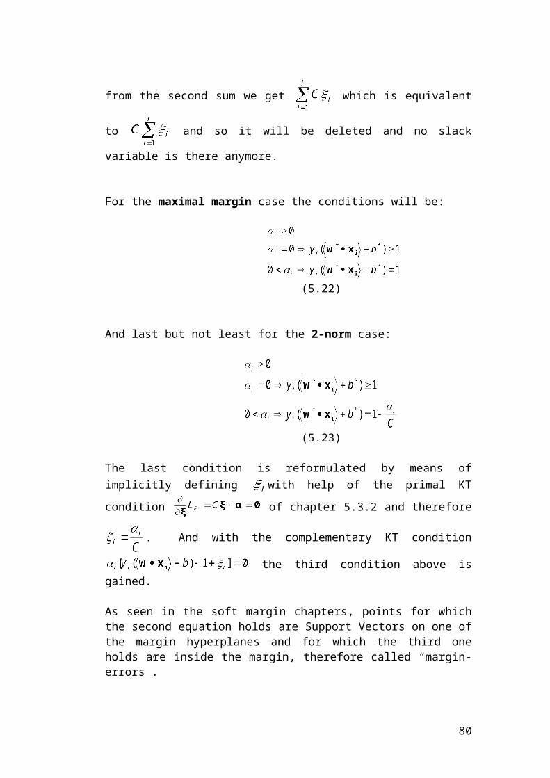
Chapter 8

Multiclass Classification

Up to now the study has been limited to the two-class case, called the bin-ary case, where only two classes of data have to be separated. However, in real-world problems there are in general classes to deal with. The training set still consists of pairs where but now

with i = 1 … l. The first straightforward idea will be to re-duce the Multiclass problem to many two-class problems, so each result-ing class is separated from the remaining ones.

8.1 One-Versus-Rest (OVR)

So as mentioned above the first idea for a procedure to construct a multi-class classifier is the construction of n two-class classifiers with following decision functions: ; k = 1…n (8.1)

This means that the classifier for class k separates this class from all other classes:

+1 if x belongs to class k -1 otherwise

So the step-by-step procedure starts with class one: construct first binary classifier for class 1 (positive) versus all others (negative), class 2 versus all others, ……., class k (=n) versus all others.

The resulting combined OVR decision function chooses the class for a sample that corresponds to the maximum value of k binary decision func-tions (i.e. the furthest “positive” hyperplane). For clarification see figure 8.1 and table 8.1. This whole first approach to gain a Multiclass classifier is computationally very expensive, because there is need of solving n

80

quadratic programming (QP) optimization problems of size l (training set size) now. As an example consider a three-class problem with linear ker-nel introduced in figure 8.1. The OVR method yields a decision surface di-vided by three separating hyperplanes (the dashed lines). The shaded re-gions in the figure correspond to tie situations, where two or none classifi-ers are active, i.e. vote positively at the same time (also see table 8.1).

Figure 8.1: OVR applied to a three-class (A, B, C) example with linear kernel

Now consider the classification of a new unseen sample (hexagonal in fig-ure 8.1) in the ambiguous region 3. This sample receives positive votes from both the A-class and C-class binary classifiers. However the distance of the sample from the “A-class-vs.-all” hyperplane is larger than from the “C-class-vs.-all” one. Hence, the sample is classified to belong to the A class.In the same way the ambiguous region 7 with no votes is handled.So the final combined OVR decision function results in the decision sur-face separated by the solid line in figure 8.1. Notice however that this final decision function significantly differs from the original one, which corres-ponded to the solution of k (here 3) QP optimization problems. The major drawback here is therefore that only three points (black balls in figure 8.1) of the resulting borderlines coincide with the original ones, calculated by the n Support Vector Machines. So it seems that the benefits of maximal

81

margin hyperplanes are lost. Summarized it can be said that this is the simplest Multiclass SVM method [Krs99 and Stat].

Region

Decision of the classifier Resulting

classA vs. B and C

B vs. A and C

C vs. A and B

1 - B C ?2 - - C C3 A - C ?4 A - - A5 A B - ?6 - B - B7 - - - ?

Table 8.1: Three binary OVR classifiers applied to the corresponding example (figure

8.1). The column “Resulting class” contains the resulting classification of each region.

Cells with “?” correspond to tie situations when two or none classifier are active at the

same time. See text for how ties are resolved.

8.2 One-Versus-One (OVO)

The idea behind this approach is to construct a decision function for each pair of classes (k, m) ; k, m = 1 … n:

+1 if x belongs to class k

-1 if x belongs to class m

So in total there are pairs, because this technique involves

the construction of the standard binary classifier for all pairs of classes. In other words, for every pair of classes, a binary SVM is solved with the un-derlying optimization problem to maximize the margin. The decision func-tion therefore assigns an instance to a class, which has the largest num-ber of votes after the sample has been tested against all decision func-

tions. So the classification now involves comparisons and in

82

each one the class to which the sample belongs in that binary case, get’s a “1” added to its’ number of votes (“Max Wins” strategy). Sure that there can still be tie situations. In such a case, the sample will be assigned based on the classification provided by the furthest hyperplane as in the OVR case [Krs99 and Stat]. As some researchers have proposed, this can be simplified by choosing the class with the lowest index when a tie occurs, because even then the results are still mostly accurate and approximated enough [Lin03] without additional computation of distances. But this has to be verified for the problem at hand.

The main benefit of this approach is that for every pair of classes the op-timization problem to deal with is much smaller, i.e. in total there is only need of solving n(n-1)/2 QP problems of size smaller than l (training set size), because there are only two classes involved and not the whole train-ing set in each problem as in the OVR approach.

Again consider the three-class example from the previous chapter. Using the OVO technique with a linear kernel, a decision surface is divided by three separate hyperplanes (dashed lines) obtained by the binary SVMs (see figure 8.2). The application of “Max Wins” strategy (see table 8.2) res-ults in the division of the decision surface into three regions (separated by the thicker dashed lines) and the small shaded ambiguous region in the middle.

After the tie-braking strategy from above (furthest hyperplane) applied to the ambiguous region 7 in the middle, the final decision function becomes the solid black lines and the thicker dashed ones together. Notice here that the final decision function does not differ significantly from the original one corresponding to the solution of n(n-1)/2 optimization problems. So the main advantage here in contrast to the OVR technique is the fact, that the final borderlines are parts of the calculated pair wise decision func-tions, which was not the case in the OVR approach.

83

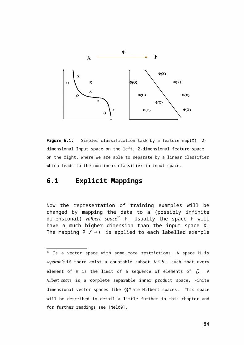
Figure 8.2: OVO applied to the three class example (A, B, C) with linear kernel

Region

Decision of the classifier Resulting

classA vs. C B vs. C A vs. B

1 C C B C2 C C A C3 A C A A4 A B A A5 A B B B6 C B B B7 C B A ?

Table 8.2: Three binary OVO classifiers applied to the corresponding example (figure 8.2). The

column “Resulting class” contains the resulting classification of each region according to “Max

Wins” strategy. The only cell with “?” corresponds to the tie situation when three classifier are act -

ive at the same time. See text for how this tie is resolved.

84

8.3 Other Methods

The above methods are only some of the ones usable for Multiclass SVMs, but they are the most intuitive ones. Other methods are e.g. the us-age of binary decision trees which are nearly the same as the OVO method. For details on them see [Pcs00].

Another method was proposed by Weston and Watkins (“WW”) [Stat and WeW98]. In this technique the n-class case is reduced to solving a single quadratic optimization problem of the new size (n-1)*l which is identical to binary SVMs for the case n = 2. There exist some speed-up techniques for this optimization problem, called decomposition [Stat], but the main disad-vantage is that the optimality of this method is not yet proven.

An extension to this was given by Cramer and Singer (“CS”). There the same problem of the WW approach has to be solved, but they managed to reduce the number of slack variables in the constraints of the optimization problem, and hence it is computationally cheaper. Also there exist some techniques known as decomposition for speed-up [Stat]. But unfortunately, same as above, the optimality has not been demonstrated yet.

But which method is suitable now for a certain problem ?

As shown in [WeW98] and other papers the optimal technique is mostly the WW approach. This method has shown the best results in comparison to OVO, OVR and the binary decision trees. But as this method is not proven yet to be optimal and there is some need of reformulation of the problem, it is not easy to implement. As a good compromise the OVO method could be chosen. This method is mainly used by the actual implementations and has shown to produce good results [Lin03].

Vapnik himself has used the OVR method, what is mainly attributed to the smaller steps for computing. Because in the OVR case there is only a need for constructing n hyperplanes, one for each class, while in the OVO case there are instead n(n-1)/2 ones to compute. So the use of the OVR technique decreases the computational effort by a factor of (n-1)/2. The main advantage, compared with the WW method, is that in OVR (as in OVO) one is able to choose different kernels for each separation, which is not possible in the WW case, because it is a joint computation [Vap98].

85

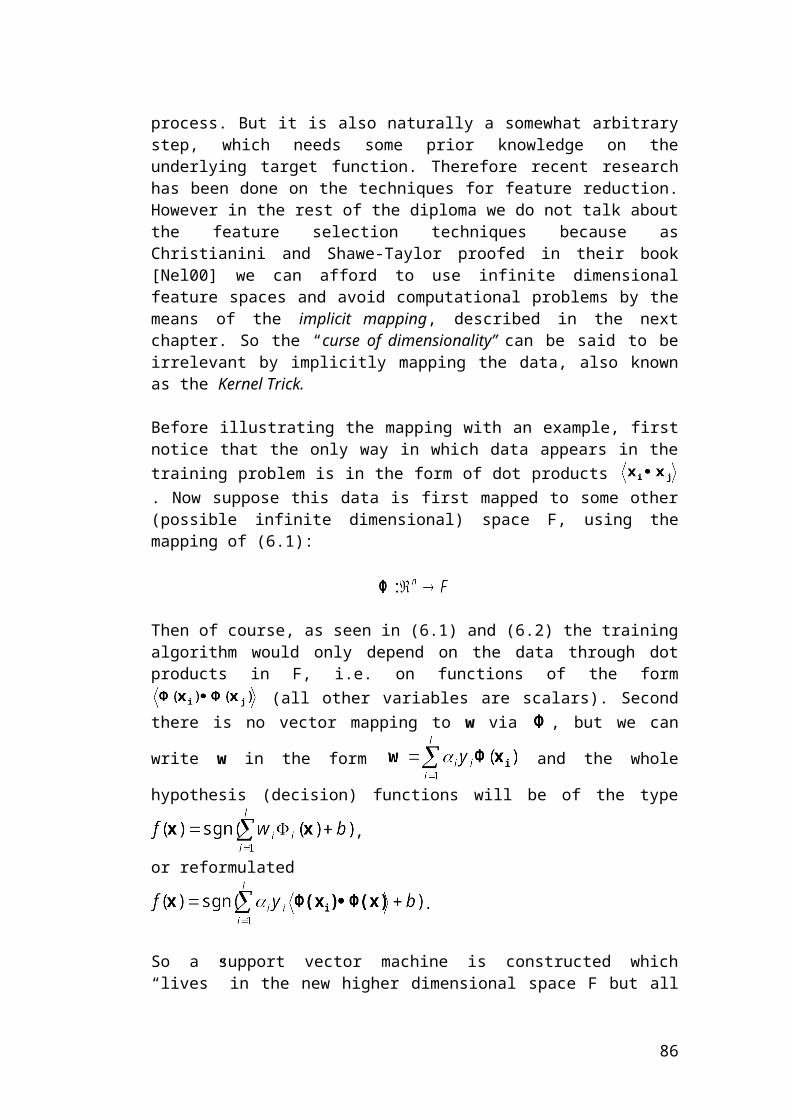
Part III

Implementation

86

Chapter 9

Implementation Techniques

In the previous chapters it was showed that the training of Support Vector Machines can be reduced to maximizing a convex quadratic function with subject to linear constraints (see chapter 5.5.1). Such convex quadratic functions have only one local maxima (the global one) and their solution can always be found efficiently. Furthermore the dual representation of the problem showed how the training could be successfully performed even in very high dimensional feature spaces. The problem of minimizing differentiable functions of many variables has been widely studied, especially in the convex case, and most of the stand-ard techniques can be directly applied to SVM training. However there ex-ist specific techniques to exploit particular features of this problem. For ex-ample the large size of the training set is a formidable obstacle to a direct use of standard techniques, since just storing the kernel matrix requires a memory space that grows quadratically with the sample size.

9.1 General Techniques

A number of optimization techniques have been devised over the years, and many of them can be directly applied to quadratic programms. As ex-amples think of the Newton method, conjugate gradient or the primal dual interior-point methods. They can be applied to the case of Support Vector Machines straightforward. Not only this, they can also be considerably simplified because of the fact, that the specific structure of the objective function is given. Conceptually they are not very different from the simple gradient ascent16

strategy, known from the Neural Networks. But many of this techniques re-quire that the kernel matrix is stored completely in memory. The quadratic form in (5.18) involves a matrix that has a number of elements equal to the square of the number of training examples. This matrix then e.g. cannot fit into a memory of size 128 Megabytes if there are more than 4000 training examples (assuming each element is stored as an 8-byte double precision 16 For an adaption to SVMs, see [Nel00]

87

number). So for large size problems the approaches described above can be inefficient or even impossible. So they are used in conjunction with the so called decomposition techniques (“Chunking and Decomposition”, for explanation see [Nel00]). The main idea behind this methods is to sub-sequently optimize only a small subset of the problem in each iteration.The main advantages of such techniques is that they are well understood and widely available in a number of commercial and freeware packages. These were mainly used for Support Vector Machines before special al-gorithms were developed. The most common algorithms were, for ex-ample, the MINOS package from the Stanford Optimization Laboratory (hybrid strategy) and the LOQO package (primal dual interior-point method). In contrast to these, the quadratic program subroutine qp provided in the MATLAB optimization toolbox is very general but the routine quadprog is significantly better than qp.

9.2 Sequential Minimal Optimization (SMO)

The algorithm used in nearly any implementation of SVMs in a slightly changed manner and in the one of this diploma thesis, too, is the SMO al-gorithm. It was developed by John C. Platt [Pla00] and its’ main advantage besides being one of the most competitive is the fact that it is simple to im-plement. The idea behind this algorithm is derived by taking the idea of the decom-position method to its extreme and optimizing a minimal subset of just two points at each iteration. The power of this approach resides in the fact that the optimization problem for two data points admits an analytical solution, eliminating the need to use an iterative quadratic program optimizer as part of the algorithm. So SMO breaks the large QP problem into a series of smallest possible QP problems and solves them analytically, which avoids using a time-consuming numerical QP optimization as an inner loop. Therefore the amount of memory required for SMO is linear in the training set size, no more quadratically, which allows SMO to handle very large training sets. The computation time of SMO is mainly dominated by SVM evaluation, which will be seen below.

The smallest possible subset for optimization involves two Lagrange multi-pliers, because the multipliers must obey the linear equality constraint (of

5.20) and therefore updating one multiplier , at least one

other multiplier ( , and ) has to be adjusted in order to keep the condition true.

88

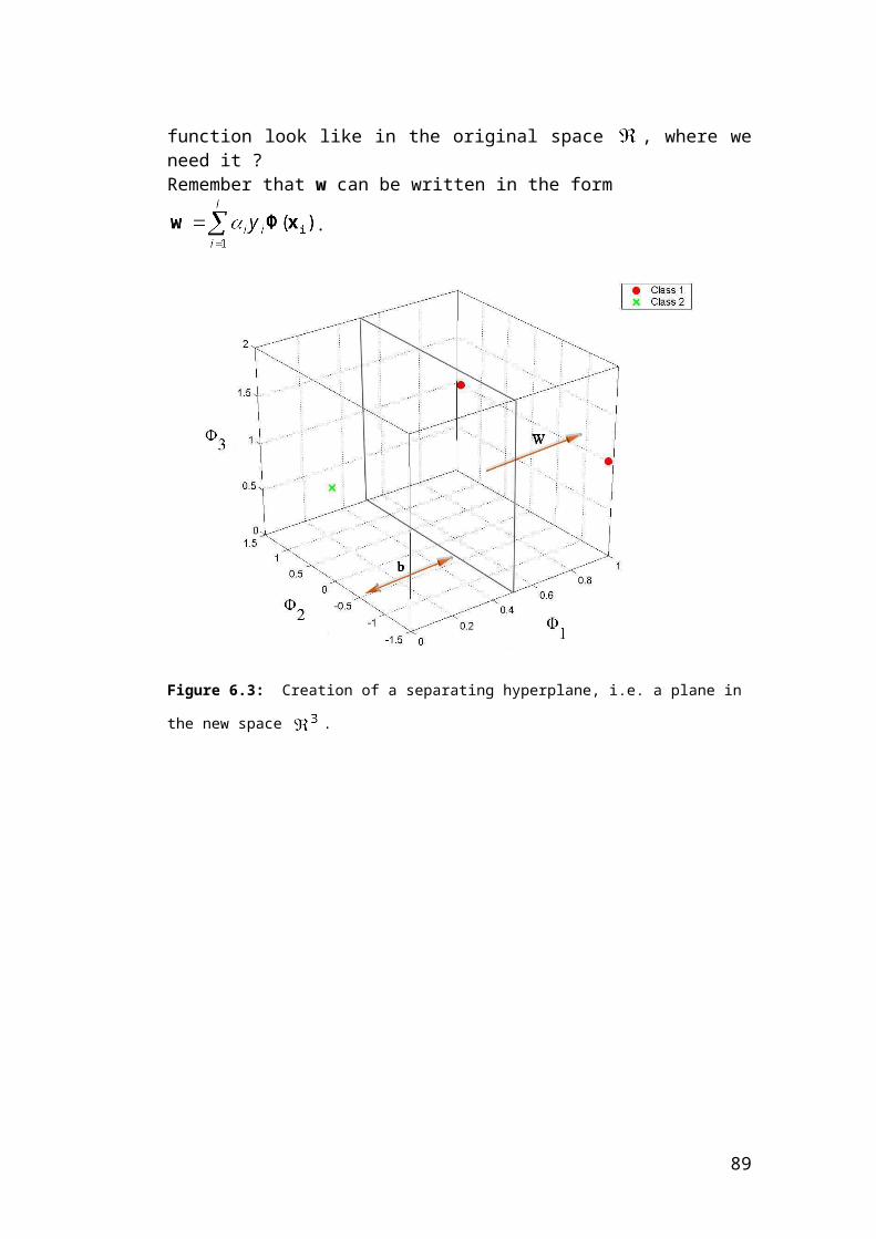
At every step, SMO chooses two Lagrange multipliers to jointly optimize, finds the optimal values for them, and updates the SVM to reflect the new optimal values.So the advantage of SMO, to repeat it again, lies in the fact that solving for two Lagrange multipliers can be done analytically. Thus, an entire inner it-eration due to numerical QP optimization is avoided. Even though more optimization sub-problems are solved now, each sub-problem is so fast solvable, such that the overall QP problem can be solved quickly (compar-ison between the most commonly used methods can be found in [Pla00]).In addition, SMO does not require extra matrix storage (ignoring the minor amounts of memory required to store any 2x2 matrices required by SMO). Thus, very large SVM training problems can fit even inside of the memory of an ordinary personal computer.The SMO algorithm mainly consists of three components:

An analytic method to solve for the two Lagrange multipliers A heuristic for choosing which multipliers to optimize A method for computing the bias b

As even mentioned in chapter 5.2.1 the computation of the bias b can be problematic, when simply taking the average value for b after summing up all calculated b’s for each i. This was shown by [Ker01]. The main problem arising when using an averaged value of the bias for recalculation in the SMO algorithm is, that the convergence speed of it is not guaranteed. Sometimes it is slower and sometimes it is faster. So Keerthi suggested an improvement for the SMO algorithm where two threshold values bup and blow are used instead of one. It has been shown in this paper that the mod-ified SMO algorithm is more efficient on any tested dataset in contrast to the original one. The speed-up is significant !But as a first introduction the original SMO algorithm will be used here and can be extended later. Before continuing, one disadvantage of the SMO algorithm should be stated here. In the original form implemented in nearly any toolbox, it cannot handle the 2-norm case. Because the KT-conditions are others, as can be seen in chapter 5.5.2. Therefore nearly any toolbox, which wants to implement the 2-norm case, uses optimization techniques mentioned above. Only one implements the 1- and 2-norm case at the same time with an extended form of the SMO algorithm (LibSVM by Chih-Jen Lin). The 2-norm case will also be added to the developed SMO al-gorithm in this diploma thesis.As it will be seen, SMO will spend most of the time evaluating the decision function, rather than performing QP, it can exploit data sets which contain substantial number of zero elements. Such sets will be called sparse.

9.2.1 Solving for two Lagrange Multipliers

89

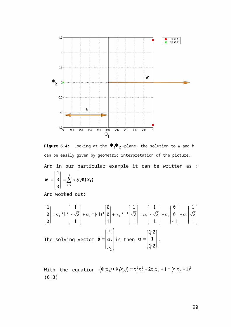
Maximize

subject to

i = 1…l

First recall the general mathematical formulated problem:

With the following KT conditions fulfilled, if the QP problem is solved for all i (for maximal-margin and 1-norm):

For convenience, all quantities referring to the first multiplier will have a subscript 1 and those referring to the second a subscript 2. Without the other subscript “old”, they are meant to be the just optimized values “new”.

For initializing is set to zero.In order to take the step to the overall solution two ’s are picked and SMO calculates the constraints on these two multipliers and then solves for the constrained maximum. Because there are only two constraints now, they can be easily displayed in two dimension (see figure 9.1). The constraints cause the Lagrange multipliers to lie inside a box,

while the linear equality constraint causes them to lie on a diag-

onal line. Thus, the constrained maximum of the objective function must lie on a diagonal line segment (explanation in figure 9.1 and following pages).In other words, to not violate the linear constraint on the two multipliers they must fulfil: (lie on a line) in the box constrained by .So this one-dimensional problem resulting from the restriction of the ob-jective function to such a line can be solved analytically.

90

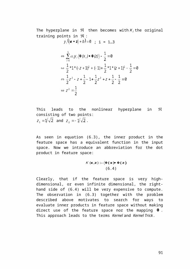
Figure 9.1: Two cases of optimization: and . The two Lagrange multipli-

ers chosen for subset optimization must fulfil all of the constraints of the full problem. The

inequality constraints cause them to lie inside a box and the linear equality constraint

causes them to lie on a diagonal line. Therefore, one step of SMO must find an optimum

of the objective function on a diagonal line segment. In this figure, , which

is a constant that depends on the previous values of , and . (

)

Without loss of generality, the algorithm first computes the second multi-plier and computes the ends of the diagonal line segments in terms of this one. So it is successively used to obtain . The bounds on the new multiplier can be formulated more restrictive with use of the linear con-straint and the equality constraint (also see figure 9.2). But first recall for

each : and also the linear constraint has to hold: .

Using the two actual multipliers to be optimized we write

and therefore where .

There are two cases to consider (remember ):

91

Figure 9.2: Case 1: . , and the two lines, indicating the cases where

or

Case 1: then (9.1)

Case 2: then (9.2)

Then let , then the two above equations can be written as

(9.3)

and before optimization .

Then the end points of the searched diagonal line (figure 9.2 and 9.3) can be expressed with help of the old, possibly not optimized values:

Case 1:

L ( at the lower end point) is: max (0, ) = max (0, )

H ( at the higher end point) is: min (C, C ) = min (C, C + )

92

where, if : L = max (0, )H = min (C, )

and if : L = max (0, )H = min (C, )

Figure 9.3: Case 2: . , and the two lines, indicating the cases where

or

Case 2:

L ( at the lower end point) is: max (0, ) = max (0, )

H ( at the higher end point) is: min (C, ) = min (C, )

As a summary the bounds on are:

(9.4)

93

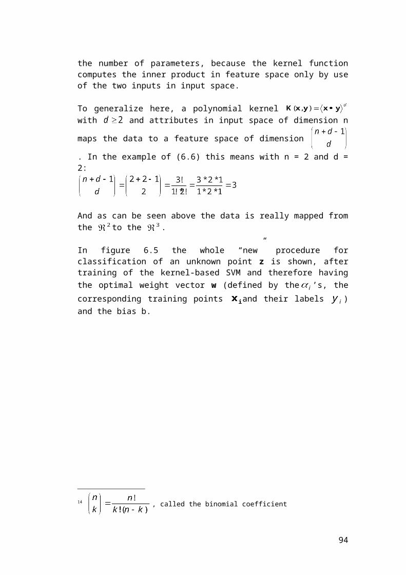
At a first glance, this only appears to be applicable to the 1-norm case, but treating C as infinite for the hard-margin case reduces the constraints on the interval [L, H]:

where, if : L = max (0, )

only lower bounded and if :

L = 0H =

Now that the other ’s are assumed fixed, the objective function = can be rewritten (as abbreviation = is written

here as ):

“const.” are the parts dependable on the multipliers not optimized in this step, so they are regarded as constant values simply added. Now for sim-plification assume the following substitutions:

, , and

As in figure 9.1, assume and with the equality constraint we get , multiplied with leading to ( )

where .

And resubstituting all these relations back into the formula becomes:

94

; i = 1, 2

Where is

And by using the help of to only have a function dependable on :

To find the maximum of this function there is need for the first and second derivate of W with respect to :

where

The following new notation will simplify the statement. is the current hypothesis function determined by the values of the actual vector and the bias b at a particular stage of learning. So the following new introduced element E is the difference between the function output (classification by the up to now trained machine) and the target classifica-tion (given by the supervisor in the training set) on the training points or

. Meaning this is the training error on the ith example.

(9.5)This value may be large even if a point is correctly classified. As an ex-ample if and the function output is = 5, the classification is cor-rect but = 4.

Recall the substitution so from 9.5 is written as:

95

and so

(9.6)

and so

(9.7)

At the maximal point the first derivate is zero and the second one has

to be negative. Hence

And with equations 9.6 and 9.7 this becomes (remember and ):

96

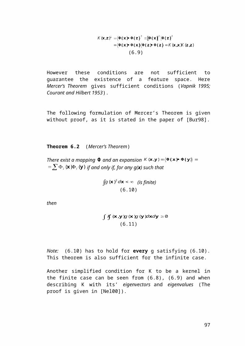
H if

= if

L if

So the new multiplier can be expressed as:

(9.8)

This is the unconstrained maximum, so this has to be constrained to lie within the ends of the diagonal line, meaning (see figure 9.1):

(9.9)

The value of is obtained from equation and therefore

(9.10)

As stated above, the second derivate has to be negative to ensure a max-imum. But under unusual circumstances it will not be negative. A zero second derivate can occur if more than one training example has the same input vector . In any event, SMO will work even if the second deriv-ate is not negative, in which case the objective function W should be eval-uated at each end of the line segment. Then SMO uses the Lagrange mul-tipliers at the end point, which yields the highest value of the objective function. These circumstances are regarded and “solved” in the next sub-chapter about choosing the Lagrange multipliers to be optimized.

9.2.2 Heuristics for choosing which Lagrange Multipli-ers to optimize

The SMO algorithm is based on the evaluation of the KT conditions. Be-cause when every multiplier fulfils these conditions of the problem, the

97

solution is found. These KT conditions normally are verified to a certain tolerance level . As Platt mentioned in his paper, the value of is typic-ally in the range of to implying that e.g. outputs on the positive (+1) margin are between 0.999 and 1.001. Normally this tolerance is enough when using an SVM for recognition. Applying higher accuracy the algorithm will not converge very fast. There are two heuristics used for choosing the two multipliers to optimize. The choice of the first heuristic for provides the outer loop of the SMO algorithm. This loop first iterates over the entire training set, determining whether an example violates the KT conditions. If so, then this example is immediately chosen for optimization. The second example, and therefore the candidate for is found by the second choice heuristic and then these two multipliers are jointly optimized. At the end of this optimization, the SVM is updated and the algorithm resumes iterating over the training examples looking for KT violators. To speed up the training, the outer loop does not always iterate over the entire training set. After one pass through the training set, the outer loop only iterates those examples whose Lag-range multipliers are neither 0 nor C (the non-bound examples). Then again, each example is checked against the KT conditions, and violating ones are chosen for immediate optimization and update. So the outer loop makes repeated passes over the non-bound examples until all of them ob-tain the KT conditions within the tolerance level . Then the outer loop iter-ates over the whole training set again to find violators. So all in all the outer loop keeps altering between single passes over the whole training set and multiple passes over the non-bound subset until the entire set obeys the KT condition within the tolerance level . At this point the al-gorithm terminates.Once the first Lagrange multiplier to be optimized is chosen, the second one has to be found. The heuristic for this one is based on maximizing the step that can be taken during joint optimization. Evaluating the Kernel function for doing so will be time-consuming, so SMO uses an approxima-tion on the step size by using equation (9.8). So the maximum possible step size is the one having the biggest value . To speed up, a cached error value E is kept for every non-bound example from which SMO chooses the one to approximately maximize the step size. If is positive, then the example with minimum error is chosen. If is negat-ive, then the example with largest error is chosen. Under unusual circumstances, as the ones remarked at the end of the last sub-chapter (two identical training vectors), SMO cannot make positive progress using this second choice heuristic. To avoid this, SMO uses a hierarchy of second choice heuristics until it finds a pair of multipliers, making positive progress. If there is no positive progress using above ap-proximation, the algorithm starts iterating through the non-bound examples at a random position. If none of them makes positive progress the al-gorithm starts iterating through the entire training set at a random position to find a suitable multiplier that will make positive progress in the joint optimization. The randomness in choosing the starting position is used to

98

avoid bias towards examples stored at the beginning of the training set. In very extreme degenerative cases, a second multiplier making positive pro-gress cannot be found. In such cases the first multiplier is skipped and a new one is chosen.

9.2.3 Updating the threshold b and the Error Cache

Since the solving for the Lagrange multipliers does not determine the threshold b of the SVM, and there is need for updating the value of the er-ror cache E at the end of each optimization step, the value of b has to be re-evaluated after each optimization. So b is re-computed after each step, so that the KT conditions are fulfilled for both optimized examples.

Now let be the output of the SVM with the old and :

(9.11)

(9.12)

As in figure 9.4, if the new is not at the bounds, then the output of the SVM after optimization on example 1 will be , its label value. And there-fore:

(9.13)

And substituting (9.13) and (9.11) into (9.12) :

(9.14)

Similarly obtaining an equation for , such that the output of the SVM after optimization is when is not at the bounds:

(9.15)

When both and are valid, they are equal (see figure 9.4 again).When both new calculated Lagrange multipliers are at the bound and if L is not equal to H, then the interval describes all threshold consist-

99

ent with the KT conditions. Then SMO chooses b to be . This

formula is only valid, if b is subtracted from the weighted sum of the ker -nels, not added. If one multiplier is at the bound and the other one not, then the value of b calculated using the non-bound multiplier is used as the new updated threshold. As mentioned above, this step is regarded as problematic by [Ker01]. But to avoid this, the original SMO algorithm dis-cussed here has to be modified in its’ whole and therefore only a reference to the improved algorithm is given here. The modified pseudo code will be stated together with the original one in the appendix.

As seen in the former chapter, a cached error value E is kept for every ex-ample whose Lagrange multiplier is neither zero nor C (non-bound). So if a Lagrange multiplier is non-bound after being optimized, its’ cached error is zero (it is classified correctly). Whenever a joint optimization occurs, the stored error of the other not involved multipliers have to be updated using the following equation:

And re-substituted this becomes:

(9.16)

100

Figure 9.4: Threshold b when both ’s are bound (== C). The support vectors A and B

give the same threshold b, that is the distance of the optimal separating hyperplane from

the origin. Point D and E give and respectively. They are error points within the

margin. The searched b is somewhere between and .

Overall, when an error value E is required by the SMO algorithm, it will look it up in the error cache if the corresponding Lagrange multiplier is not at bound. Otherwise, it will evaluate the current SVM decision function (classify the given point and compare it to the given label) based on the current ’s.

9.2.4 Speeding up SMO

There are certain points in the SMO algorithm, where some useful tech-niques can be considered to speed up the calculation. As said in the sum-mary on linear SVM, it is possible there to store the weight vector directly, rather than all of the training examples that correspond to non-zero Lag-range multipliers. But this optimization is only possible for the linear kernel. After the joint optimization succeeded, the stored weight vector must be updated to reflect the new Lagrange multipliers found. This update is easy, due to the linearity of the SVM:

101

This is a speed-up because much of the computation time in SMO is spent to evaluate the decision function, and therefore speeding up the decision function speeds up SMO. Another optimization that can be made is using the sparseness of the input vectors. Normally, an input vector is stored as a vector of floating point numbers. A sparse input vector (with zeros in it) is stored by the meaning of two arrays: id and val. The id array is an integer array storing the location of the non-zero inputs, while the val array is a floating point array storing the corresponding non-zero values. Then the very often used computation of the dot product between such stored vec-tors (id1, val1, length=num1) and (id2, val2, length=num2) can be done quickly, as shown in the pseudo code below:

p1 = 0, p2 = 0, dot = 0

while (p1 < num1 && p2 < num2){ a1 = id1[p1], a2 = id2[p2]

if (a1 == a2) { dot += val1[p1]*val2[p2] p1++, p2++ }

else if (a1 > a2) p2++

else p1++}

This can be used to calculate linear and polynomial kernels directly. Gaussian kernels can also use this optimization through the usage of the following identity:

To speed up more in the Gaussian case, for every input the dot product with itself can be pre-computed.

Another optimization technique for linear SVMs regards the weight vector again. Because it is not stored as a sparse array, the dot product of the weight vector with a sparse input vector (id, val) can be expressed as:

102

And for binary inputs storing the array val is not even necessary, since it is always 1. Therefore the dot product calculation in the pseudo code above becomes a simple increment and for a linear SVM the dot product of the weight vector with a sparse input vector becomes:

As mentioned in Platt’s paper there are more speed-up techniques that can be used but they will not be discussed in detail here.

9.2.5 The improved SMO algorithm by Keerthi

In his paper [Ker01] Keerthi points out some difficulties encountered in the original SMO algorithm by explicitly using the threshold b for checking the KT conditions. His modified algorithm will be stated here as Pseudo-Code with a little explanation, but for further details please refer to Keerthi’s pa-per.Keerthi uses some new notations:Define . Now the KT conditions can be expressed as:

and these can be written as:

where

And now to check if the KT conditions hold, Keerthi also defines:

103

(A)17

(B)

The KT conditions then imply and similarly and .

These comparisons do not use the threshold b !

As an added benefit, given the first , these comparisons automatically find the second multiplier for joint optimization. The pseudo code, as it can be found in Keerthi’s paper, can be found in appendix D.

As seen in the pseudo code and in Keerthi’s paper, there are two modific-ations on the SMO algorithm. Both were tested in the paper on different datasets and showed a significant speed-up in contrast to the original SMO algorithm by Platt. Also they overcome the problem arising when only using a single threshold (an example, why there are arising problems can also be found in Keerthi’s paper). As a conclusion on all tests Keerthi showed that the second modifications fares better overall.

9.2.6 SMO and the 2-norm case

As stated before, the SMO algorithm is not able to handle the 2-norm case without altering the code. Recall that there are two differences to the max-imal margin and the 1-norm case: First the addition of 1/C to the diagonal of the kernel matrix and second the altered KT conditions, which are used in SMO as the stopping criterion:

And as the original SMO algorithm tests the KT conditions only in the outer loop when selecting the first multiplier to optimize, this is the point to alter. Also the kernel evaluation has to be extended to add the diagonal values. In the pseudo-code above, the checking of the KT conditions is processed by:

E2 = SVM output on point[i2] - y2 (check in error cache)r2 = E2*y2

17 (A) and (B) are links to the pseudocode in the appendix

104

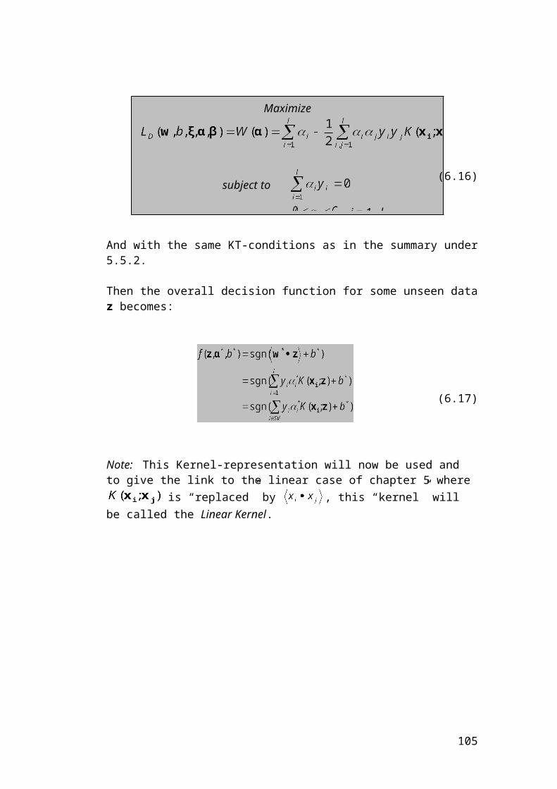
if ((r2 < -tol) || (r2 > tol && alph2 > 0))

where r2 is the same as . So the KT conditions are tested against and , where 0 is replaced by the tolerance “tol”. So for the 2-norm case the test is rewritten as:

E2 = SVM output on point[i2] - y2 (check in error cache)r2 = E2*y2 + alph2/C

if ((r2 < -tol && alph2 < C) || (r2 > tol && alph2 > 0))

Second, as in the maximal margin case, the box constraint on the multipli-ers has to be removed, because they are no longer upper bounded by C.

And last but not least, the bias has to be calculated only using alphas ful-

filling the equation .

9.3 Data Pre-processing

As one can read in [Lin03] they have some propositions on the handling of the used data.

9.3.1 Categorical Features

SVMs require that each data instance is represented as a vector of real numbers. Hence, if there are categorical attributes, they have to first be converted into numeric data. Cheng recommends to use m numbers for representing an m-category attribute. Then only one of the m numbers is one, and the others are zero. Consider the three category attribute {red, green, blue} which then can be represented as (0,0,1), (0,1,0) and (1,0,0). Cheng’s experience indicates that if the number of values in an attribute is not too many, this coding might be more stable than using a single number to represent a categorical attribute.

9.3.2 Scaling

105

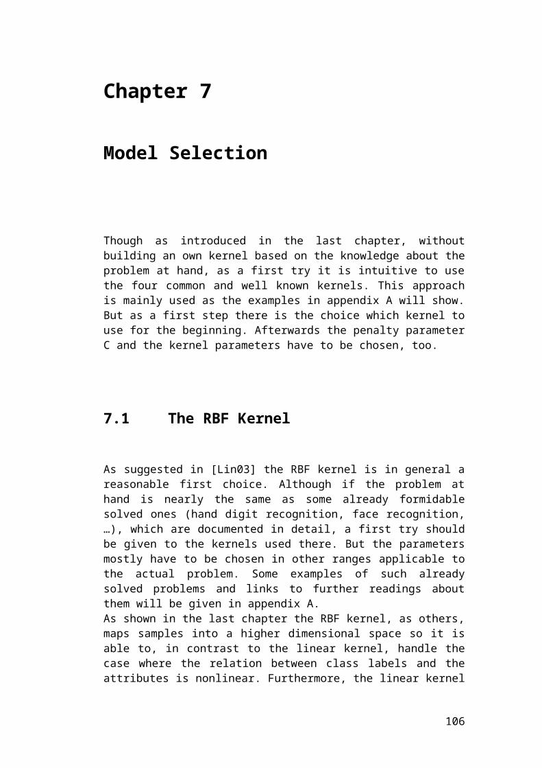
Scaling the data before applying it to an SVM is very important. [Lin03] ex-plains why the scaling is so important, and most of these considerations also apply to SVMs.The main advantage is to avoid attributes in greater numeric ranges dom-inating those in smaller numeric ranges. Another advantage is to avoid nu-merical difficulties during the calculation. Because kernel values usually depend on the inner products of feature vectors, large attributes may cause numerical problems. So Cheng recommends linearly scaling each attribute to the range of [-1, +1] or [0, 1]. In the same way, the testing data then has to be scaled before testing it on the trained machine. In this diploma thesis the most used scaling to [-1, +1] is used and the ac-cording formula for scaling an input x in this interval with length two is:

The components of and input x:= (x1 … xn)T are linearly scaled to the inter-val [-1, +1] with a length l of two by applying:

with . The scaling has to be done for each feature separately. So the min- and max-values are taken, regarding the current feature in each vector. To go in detail, the reason for doing this is follows:

Imagine a vector of 2 features (2-dimensional), the first has a value of 5, the second of 5000. Assume the other vectors behave the same way. So the first feature would not have a very great impact on distinguishing between the classes, because the change in feature one is numerically very small in contrast to that of feature two, whose numbers are in a much higher range.

Other long studied methods for scaling the data and showing very good results use the co-variance matrix from the Gaussian theory.

9.4 Matlab Implementation and Examples

This chapter is intended to show some examples and to get an impression how the different tuneable values, such as the penalty C, the kernel para-meters and the choice of maximal margin, 1-norm or 2-norm, affect the resulting classifier.

The implementation in Matlab with the original SMO algorithm can be found here together with the training sets (these files were used for mak-ing the following pictures possible):

106

Matlab Files\SVM\18

It should be mentioned, that the SMO implementation in Matlab is some-what very slow. Therefore nearly any Toolbox for SVMs available written in Matlab implements the SMO algorithm as C-Code and calls it in Matlab through the so-called “Mex-functions” (Interface to C/Matlab). But for ex-amining the small examples used here, the use of pure Matlab is accept-able. Later the whole code for Support Vector Machines will be implemen-ted in C++ anyway to be integrated in the “Neural Network Tool” already existent at Siemens VDO.For any upcoming visualisation the dimension of the training and test vec-tors is restricted to the two-dimensional case, because only such ex-amples are visualizeable two- and three-dimensional, to be discussable. The three-dimensional pictures will show the values calculated by the learned decision function without applying the classification by the signum function “sgn” to it on the z-axis. The boundary will be shaded too, re-spectively to the functional margin of that point. Or in other words: The darker the shading, the more the point belongs to that specific class. The pictures will give clarification on this.

9.4.1 Linear Kernel

For examples using the linear “kernel”, the linear separable cases of the binary functions OR and AND are considered (figure 9.5 and 9.6).

The dashed lines represent the margin. The size of the functional margin is indicated by the level of shading.

A test of the same machine on the XOR case results in a classification with one error because of the nature of the XOR function to be non separ-able in input space (figure 9.6).

18 A complete list with the usage and a short description of each file will be given in

chapter 10.

107

Figure 9.5: A linear kernel with maximal margin (C = inf) applied to the linear separable

case of the binary OR function.

Figure 9.6: A linear kernel with maximal margin (C = inf) applied to the linear separable

case of the binary AND function.

108

Figure 9.7: A linear kernel with soft margin (C = 1000) applied to the linearly non-separ-

able case of the XOR function. The error is 0.25 %, as one point is misclassified.

9.4.2 Polynomial Kernel

As seen before, the XOR case is non-separable in input space. Therefore the usage of a kernel mapping the data to a higher space and separating it there linearly could produce a classifier in input space, separating the data correctly. To test this, a polynomial kernel with maximal margin (C = inf) of degree two is used. The result can be seen in figure 9.8.

To get an impression on how this data becomes separable by mapping it to a higher dimensional space, the three-dimensional picture in figure 9.9 visualizes the output of the classification step before applying the signum (sgn) function to it on the z axis.

109

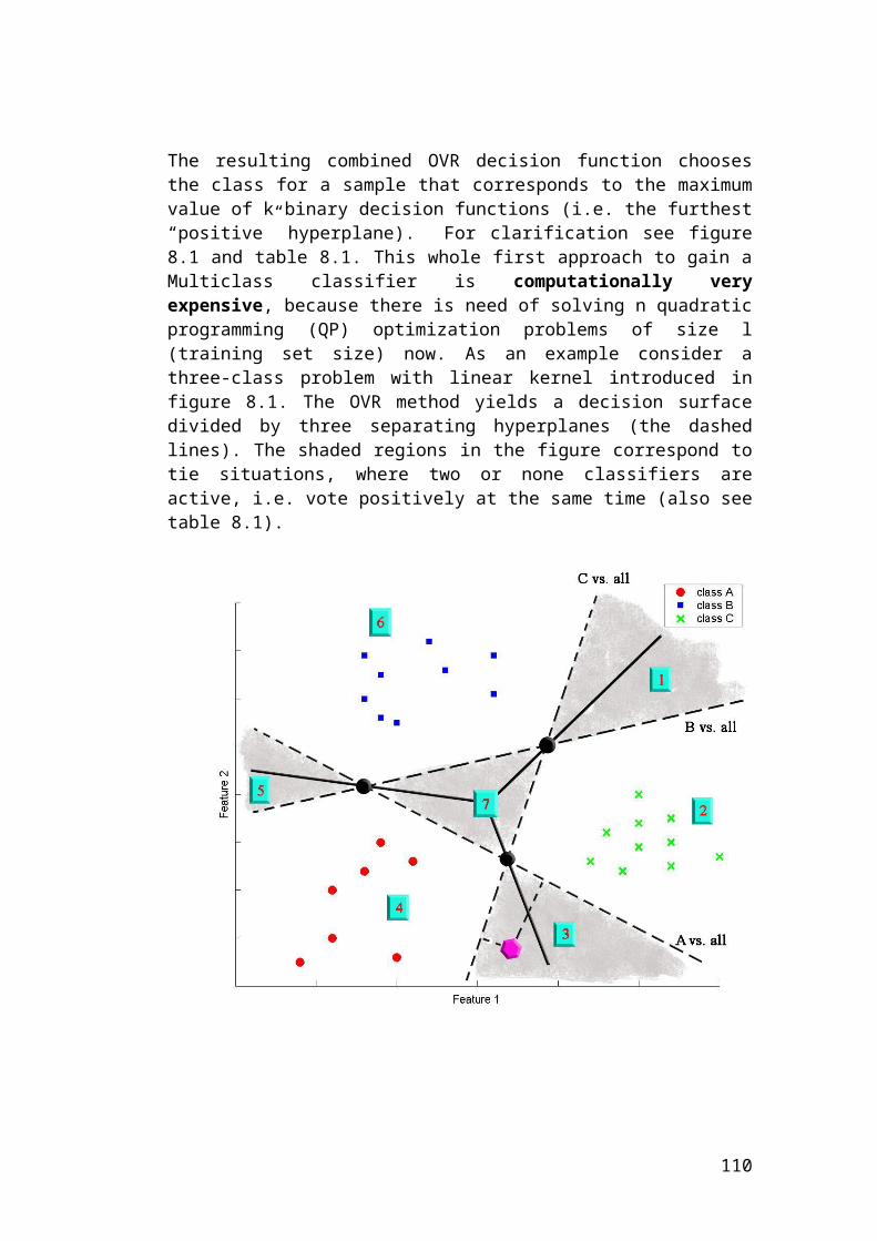
Figure 9.8: A polynomial kernel of degree 2 with maximal margin (C = inf) applied to the

XOR dataset.

110

Figure 9.9: The classificator of figure 9.8 visualized by showing the calculated value of

the classification on the z axis before the application of the signum (sgn) function.

Here one can see that the yellow regions applying to one of the classes have greater positive values and the green region applying to the other class has values lower than zero. The change of separation from one class to the other is at the zero level of the classifier output (z axis), as the signum function changes sign there.The main conclusion drawing from the pictures up to now and from further ones is, that the application of a kernel measures the similarity between the data in some way. Because regarding the last two figures again, one can see that the points belonging to the same class are mapped to the same “direction” (output values >= 0 or < 0). The upcoming pictures on the Gaussian kernel will stress this fact.

9.4.3 Gaussian Kernel (RBF)

As stated in the chapter on the kernels, if one has no idea on how the data is dependable, as a first start the Gaussian kernel(s) or in other words, the radial basis function(s) is/are a good choice.Sure in the XOR case applying this kernel will be the same as shooting with canons on sparrows, but the pictures resulting from doing so anyway, stress the fact that a kernel measures the similarity of data in some way (the resulting value before applying the signum function). Another fact is

111

that here the result of changing the sigma value (variance, “window width”, see 6.2.3) can be seen quite clear.

Figure 9. 10: The RBF kernel applied to the XOR data set with and maximal

margin (C = inf).

To see how the change of the sigma value (variance) affects the resulting classifier, compare figures 9.10 and 9.11 to figures 9.12 and 9.13. Notice the smoother and wider course of the curves at the given training points.

112

Figure 9.11: The classificator of figure 8.9 ( ), visualized by showing the calcu-

lated value of the classification on the z axis before the application of the signum (sgn)

function. Remarkable are the “Gauss curves” at the position of the four given training

points (Here the classificator is more confident that a point in that region belongs to the

specific class).

Figure 9.12: The RBF kernel applied to the XOR data set with and maximal

margin (C = inf).

113

Figure 9.13: : The classificator of figure 9.9 ( ), visualized by showing the calcu-

lated value of the classification on the z axis before the application of the signum (sgn)

function. Remarkable are the “Gauss curves” at the position of the four given training

points. But in contrast to figure 9.11 with a value of sigma they are much

smoother and “wider”, as sigma changes the “width” (Consider the affect of the variance

in Gaussian distribution).

To get an impression on how different values of the penalty parameter C (soft margin case for 0 < C < inf) affect the resulting classifier the next pic-tures illustrate this application of C. As a starting point assume the classification problem of figure 9.14, classi-fied by a SVM with a Gaussian kernel using and the maximal mar-gin concept, allowing no training errors. The resulting classification regions are not very smooth, due to the two training points lying in the midst of the other class. Therefore applying the same machine on the dataset but with the soft margin approach by applying the upper bound by setting C to five results in the classifier of picture 9.15.Here the whole decision boundary is much smoother than in the maximal margin case. The main “advantage” is the broader margin, implying a bet-ter generalization. This fact is also stressed in the figures of 9.16 and the next sub chapter.

114

Figure 9.14: A Gaussian kernel with and maximal margin (C = inf). The dashed

margins are not really “wide”, because of the two points lying in the midst of the other

class and the application of the maximal margin classifier (no errors allowed).

115

Figure 9.15: A Gaussian kernel with and soft margin (C = 5). This approach

gives smoother decision boundaries in contrast to the classifier in figure 8.14 but at the

expense of misclassifying two points now.

9.4.4 The Impact of the Penalty Parameter C on theResulting Classifier and the Margin

Now the change of the resulting classifier (boundary, margins) when ap-plying the maximal margin and the soft margin approach will be analyzed in detail.Assume the training set used in figure 9.16. The SVM used there is based on a Gaussian kernel applying the concept of the maximal margin ap-proach, allowing no training error (C = inf). As one can see, the resulting classifier does not have a very broad margin. And therefore, as stated in the Theory on Generalization in part one of this diploma thesis, this classi-fier is assumed not to generalize very well.

In contrast to this the approaches in figures 9.17 to 9.19 use the soft mar-gin optimization and result in a broader margin but this on the expense of allowing training errors. But such “errors” can also be interpreted as the classifier does not overestimate the influence of some “outliers” in the training set (because of such ones the “hill” in figure 9.16 is in the midst of where one can imagine the other class should be).

116

Figure 9.16: A SVM with a Gaussian kernel with and maximal margin (C = inf).

The resulting classifier is compatible with the training set without error, but has no broad

margin.

So these classifiers are assumed to generalize better in this case, what is the goal of a classifier:

He must generalize very well but minimize the error of classification.

As stated in chapter two another very general estimation of the generaliza-tion error of SVMs are the number of support vectors gained after training:

So small numbers of support vectors are expected to give better general-isation. Another advantage in practice is, that the fewer support vectors there are the less expensive is the computation of the classification of a point.

So to summarize, as the theory on generalization stated, a broad margin and few support vectors are indications for good generalization. So the ap-plication of the soft margin approach can be seen as a compromise between minor empirical risk and minor optimism.

117

Figure 9.17: A SVM with a Gaussian kernel with and soft margin (C = 100). No-

tice the broader margin in contrast to figure 9.16. The boundary has become smoother

and the three (four, one is a margin error, the others are “real” errors) misclassified points

do not have as much impact on the boundary as in figure 9.16.

Figure 9.18: A SVM with a Gaussian kernel with and soft margin (C = 10). No-

tice the broader margin in contrast to figure 9.16 and 9.17. The boundary is much more

smoother.

118

Figure 9.19: A SVM with a Gaussian kernel with and soft margin (C = 1). Notice

the broader margin in contrast to figure 9.16 ,9.17 and 9.18, and the much smoother

boundary.

119

Part IV

Manuals, Available Toolboxes and Summary

120

Chapter 10

Manual

As said at the beginning, one of the goals was to implement the theory into a computer program for practical usage. This program was first developed in Matlab Release 12 for better debugging and doing demanding graph-ical output. All figures from the last chapter were done with this implement-ation and after reading this chapter you should also be able to use the files created. After testing the whole theory there extensively the code was por-ted to C++ in a module to be integrated into the already existent “Neural Network Tool”.

10.1 Matlab Implementation

First the Matlab approach was used because of the better debugging pos-sibilities of the algorithm. Also the development was faster here because of the mathematical nature of the problem. But the main advantage was the graphical output already possible with Matlab.

Figure 10.1: The disk structure for all files associated with the Matlab implementation

The next table summarizes all files created for the Matlab implementation.An example on their usage can be seen after it.

121

Path File Description Remarks

Classifier

kernel_funcInternally used for ker-nel calculation

kernel_EvalEvaluate the chosen kernel function for the given data

Binary Case

Files associated with the 2-class problem

SMOImplementation of the original SMO-Algo- rithm

Multiple return values

SMO_Keerthi

Implementation of the improved SMO-Algo- rithm by Keerthi with modification 2

Multiple return values

classify_PointClassification of an un-labeled data example after training

Value without applied signum function (sgn)

Multiclass

Multiclass_SMO

Above SMO for the multiclass case

Multiple return values

Multiclass_SMO_Keerthi

Above improved SMO for the multiclass case

Multiple return values

Multi_Clas-sify_Point

Classify a point after training

Vector contain-ing all votes for each class is re-turned; still tie situations !

TestdataContains *.mat files with prelabeled test data for loading into the workspace

Util

check2ddata Internally used by “createdata”

createdata Create 2-dimensional prelabeled training data for two- and mul-

Up to now only the following calling conven-

122

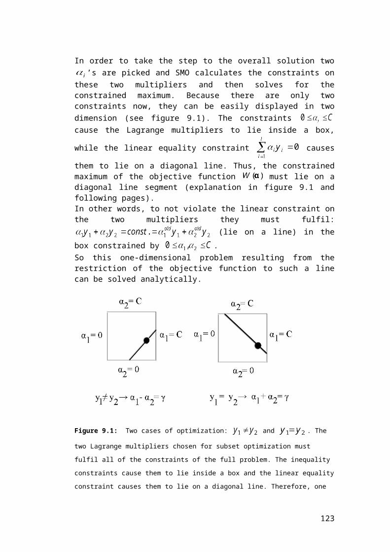
ticlass in a GUI; save-able to a file

tions are suppor-ted:

Createdata for two-class case

Createdata(‘fi-nite’, nrOf-Classes) for creating multi-class test data

linscale Scales the data to the interval [-1, +1] linearly

makeTwo-Class

If the data is not stored with labels -1 and +1 for binary clas-sification, this function rewrites them.

Calling conven-tion is:

makeTwoClass(data, label_of_one_class)

label_of_one_class is then mapped to +1 and the remain-ing ones to -1.

VisualFiles for plotting a trained classifier

Only applicable if the data/fea-ture vectors are 2-dimensional !

Binary case

For the two-class problem

svcplot2D

Two-dimensional plot of the trained classi-fier. The coloured shaded regions rep-resent the calculated value of the classifica-tion for that point BE-FORE applying the signum (sgn) function. Yellow for values >= 0 and therefore class +1 and green for values < 0 and therefore class -1. The darker the col-our the greater the value (see the legend)

The dashed lines represent the margin.

123

svcplot3D

Same as above but this three-dimensional plot visualizes the cal-culated value of the classification BEFORE applying the signum (sgn) function in the third dimension

The dashed lines represent the margin.

Multiclass

svcplot2D_Multiclass

Same as for the two-class classification above but for the prob-lem of three to a max-imum of seven classes.

Table 10.1: List of files used in the Matlab implementation and their intention

10.2 Matlab Examples

Now two examples how to use the Matlab implementation in practice.The first one is for the two-class problem and the other one shows how to train a multiclass classifier.

First call createdata or load a predefined test data set into workspace. If using the createdata function, the screen looks like figure 10.2 after gener-ating some points by left-clicking with the mouse. You can erase points by right-clicking on them and adjust the range of the axis by entering the wanted values to the right. The class could be switched in the upper right corner with the combo box. When ready, click Save and choose a file-name and location for saving the newly generated data to. Close the win-dow and load the file into the Matlab workspace. Then you should see a vector X containing the feature data and a vector y containing the labels +1 and -1 there.

124

Figure 10.2: The GUI of the createdata function after the creation of some points for two-

class classification by left-clicking on the screen.

Before training you have to specify a kernel to use. In this implementation that is done by creating a field as follows:

myKernel.name = ‘text’ optional: myKernel.param1 = value_1optional: myKernel.param2 = value_2

Values for text (the Kernel used): linear poly rbf

value_1: Not used for the linear kernel, for the polynomial one its’ the dimension of it (degree) and for the RBF/Gaussian kernel its’ the value of sigma/window width.

value_2: Only used for the polynomial kernel, where it’s the constant c added.

If none of the last two parameters is given, default values are used. There should be a new variable in the workspace called myKernel.

125

In this example we use: myKernel.name = ‘poly’myKernel.param1 = 2

Now we are ready for training. For this there are two functions available with same calling convention:

SMO SMO_Keerthi

As the names imply, the first one implements the original SMO algorithm and the second one the improved algorithm by Keerthi with modification 2. In any sense the second one should always be used, because as stated in the former part, the original SMO is very slow and could run infinitely if you choose to separate the data by meanings of hard margin but it is not sep-arable without errors. To train the classifier simply call:

[alphas bias nsv trainerror] = SMO_Keerthi(X, y, upper_bound_C, eps, tol, myKernel)

X is the training sety are the labels (+1, -1)upper_bound_C is either inf for the hard margin case or any value > 0 for the soft-margin one (here: inf)eps is the accuracy, normally set to 0.001tol is the tolerance for checking the KKT conditions, normally 0.001myKernel is the field created above

Returned values are:

alphas is the array containing the calculated Lagrange multipliersbias is the calculated biasnsv is the number of support vectors (alpha > 0)trainerror is the error rate in % on the training set

If using the original function SMO(…) there is need for another parameter after the myKernel variable: 2-norm, which is zero for using hard-margin or 1-norm soft-margin and one for using the 2-norm.

After pressing Return the training process starts and you get the overview as in figure 10.3 after the training has ended.Now if the upper calling convention is used you got two newly created vari-ables in the workspace for further usage: alphas and bias

Now the result can be visualized by using the functions svcplot2D and/or svcplot3D, as can be seen in figure 10.4 and 10.5. They have the same calling convention:

126

svcplot2D(X, y, myKernel, alphas, bias)

Where X is again the training data as before and also the labels y and myKernel. Alphas and bias are the variables gained through the training process.

Figure 10.3: After training you get the results: values of alphas, the bias, the training er-

ror and the number of support vectors (nsv)

127

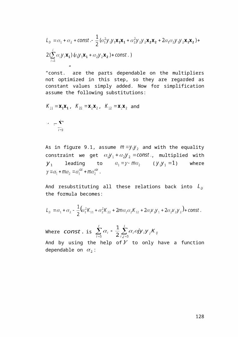
Figure 10.4: svcplot2D after the training of a polynomial kernel with degree two on the

training set created as in figure 10.2.

Figure 10.5: svcplot3D after the training of a polynomial kernel with degree two on the

training set created in figure 10.2.

The second example consist of four classes to show how multiclass classi-fication works here. Again create a training set with createdata, but now by calling (see figure 10.6):

createdata(‘finite’, 4)

128

Figure 10.6: GUI for creating a four-class problem

In this example we use a linear kernel: myKernel.name = ‘linear’After again loading the created data into workspace, getting the variables X and y, we are ready for training:

[alphas bias nsv trainerror overall_error] = Multiclass_SMO_Keerthi(X, y, upper_bound_C, eps, tol, myKernel)

The only difference here to the binary case is the additional return value of the overall error, because trainerror is the error rate of each classifier trained during the process (you have multiple ones, because the OVO-method is used).

After the training you get again the results as in figure 10.3. Now again the trained classifier(s) can be plotted:

svcplot2D_Multiclass(X, mykernel, alpha, bias, nr_of_classes)

where X is the training data, nr_of_classes is the number of classes used in training (here: 4) and the other parameters are the same as in the bin-ary case above. This plot would take a little more time to show up but in the end it looks like the one in figure 10.7.

129

Figure 10.7: svcplot2D_Multiclass called after the training of the four classes as created

in figure 10.6.

10.3 The C++ Implementation for the Neural Network Tool

The main goal of this work was the integration of the SVM module into the already existing “Neural Network Tool” created by Siemens VDO. The ap-plication GUI is shown in figure 10.8 with a test of the SVM. The tool was consisting of two integrated classifiers: The polynomial one and the Radial Basis Function classifier. It was capable of:

Train multiple instances of a classifier on separate or the same train-ing set(s)

Visualizing data of two dimensions and the trained classifier

Storing results and the parameters of a classifier for loading an already trained classifier and test it on another data set

130

Figure 10.8: The Neural Network Tool with integrated SVM. Here an overlapping training

set was trained with the Gaussian/RBF kernel with no error.

The integration of the new module was “easy” because of the already open system for further integration of new classification techniques. So the todos where the following:

Programming of a control GUI for the SVM

Programming of the algorithms themselves

Store and load procedures for the relevant parameters to load a trained classifier at a later time

Store procedures for the results of a training run

As the algorithms used have been tested extensively in Matlab they did not need any further debugging here. And as a benefit of the saved time therefore some additions were made not implemented in Matlab. For ex-ample now one is able to do a Grid Search for the upper bound C as de-

131

scribed in chapter 7.2 but without cross-validation. Algorithms implemen-ted here are the original SMO with 1- and 2-norm capabilities and the im-proved SMO by Keerthi with modification two.

The program was split into few modules, which can be seen in figure 10.9.

Figure 10.9: The UML diagram for the integration of the SVM module

In figure 10.10 the main control dialog for configuring all relevant stuff for SVM training can be seen.

At the top you see the actual file loaded for training or testing. Below on the left you can select the kernel to use (without knowledge one should start with the Gaussian/RBF one, default) and the algorithm of choice. Keerthi should be selected always because of his big advantages de-scribed in the chapters beforehand. On the right hand side all other import-ant variables are accessible, such as the upper bound C (checkbox for the hard-margin case, if deselected you can enter an upper bound by hand > 0), the kernel parameters (polynomial degree/constant or sigma for the Gaussian/RBF kernel) ,the accuracy of calculation and the tolerance for checking the KT conditions (default values here are 0.001).

132

Figure 10.10: Main control interface for configuring the important parameters for SVM

training

Remember that if you select the SMO 2-norm as algorithm, no hard-mar-gin classification is possible and therefore it is not selectable then. The in-put for the polynomial degree and sigma is shared in one edit box, indic-ated by the text next to it, which will be switched appropriate. In the lower half you can check the box next to Upper Bound C for doing a grid search over predefined values of C. This simply trains 12 classifiers with different values for the upper bound C (currently these are: and in-finity for the hard-margin case; such exponentially growing values were re-

133

commended by Lin as seen in chapter 7.2) and shows the results in a dia-log after training (see figure 10.11). Then one can select the best paramet-ers for training the classifier.

Figure 10.11: The results of a grid search for the upper bound C. From left to right it dis-

plays: Number of support vectors (NSV), Kernel parameters (unused yet), the used upper

bound C and the training error in %. So one can easily see the general development of

the training process for different values of C. Remarkable here is the fast decrease of the

NSV with increasing C. As stated in chapter 9 most of the times the fewer support vectors

there are the better the generalisation will be. All in all this search helps a lot finding the

optimal value for the upper bound. With the later implementation of the grid search for the

kernel parameters this will be a powerful tool to find the best suited parameters for the

problem at hand.

Last but not least with the Stop Learning button one can interrupt the train-ing process and at the bottom of the dialog is a progress bar to give visual feedback of the learning or testing progress.

As the Neural Network Tool is property of Siemens VDO I am not able to include source files here or on the CD, but all Matlab files are included for testing purposes.

134

10.4 Available Toolboxes implementing SVM

There are many toolboxes implemented in Matlab, C, C++, Python and many more programming languages available on the internet and free of charge for non-commercial usage. This chapter does not claim to show them all but few ones which were used during the work on this diploma. Some use alternative algorithms for solving the optimization problem arising in SVMs and others are based on modifications of SMO. All tool-boxes mentioned here are also available on the CD coming with this work.

A very good page with many resources and links can be found here:http://www.kernel-machines.org

Most toolboxes are intended for usage under Linux/Unix, but there are more and more ones ported to the Windows world. Some of them used during the work are listed here:

NAME DESCRIPTION LINK

LibSVM

A SVM library in C with a graph-ical GUI. It is the basis for many other toolboxes. The algorithm implemented here is a simplifica-tion of SMO, SVMLight and modification 2 of SMO by Keerthi.

HTTP://WWW.C-SIE.NTU.EDU.TW/~CJLIN/LIBSVM/

SVMLight

SVM in C with own algorithm. Also used in other toolboxes such as mySVM. It was tested with superior success in text cat-egorization on the Reuters data set.

HTTP://SVMLIGHT.-JOACHIMS.ORG/

Statistical Pattern Re-cognition Toolbox for Matlab

A huge toolbox for Matlab from the university of Prague. It imple-ments many algorithms not only SVM. Very comfortable because of the GUI.

HTTP://CM-P.FELK.CVUT.CZ

mySVMA toolbox in C based on the SVMLight algorithm for pattern recognition and regression.

HTTP://WWW-AI.C-S.UNI-DORTMUND.DE/SOFTWARE/MYSVM/

135

mySVM and SVMLight

The above toolbox but written in/for Visual C++ 6.0.

HTTP://WWW.CS.UC-L.AC.UK/STAFF/M.SEWELL/SVM/

OSU SVMA Matlab toolbox with the core part written as MEX code for fast implementation based on LibSVM.

HTTP://WWW.ELE-CENG.OHIO-STATE.EDU/~MAJ/OSU_SVM/

WinSVM An easy to use Windows toolbox with GUI.

HTTP://LIAMA.I-A.AC.CN/PERSONALPAGE/LBCHEN/

Torch A machine learning library written in C++ for large scale datasets.

HTTP://WWW.T-ORCH.CH/

SVMTorchSVM for classification and re-gression on large data sets based on the torch library.

HTTP://WWW.IDIAP.CH/INDEX.PHP?CONTENT=SVMTORCH&INCFILE=PAGETYPE&URLTEMPLATETYPE=3&CPATHCONTENU=PAGES/CONTENUTXT/PROJECTS/TORCH/

Table 10.2: Overview of some toolboxes available for Windows/Linux/Unix implemented

in Matlab and C/C++.

10.5 Overall Summary

This work was intended to give an introduction to how Support Vector Ma-chines can be used in the field of pattern recognition. It has been the goal to let the reader understand why it works at all and how this is achieved mathematically. The mathematical background should be understandable with minor knowledge in the fields of machine learning and optimization. So all mathematical basics important to understand Support Vector Ma-chines were described in a way such that a person from the technical branch would be able to do further research in this field without reading all mathematically written books and papers concerning Support Vector Ma-chines. This work was not intended to look in all details of the algorithms available but to get used to the basic ones. So further research could be done espe-

136

cially in the field of Multiclass classification, where the mentioned Weston and Watkins (WW) method showed very good results but is somewhat very complicated to use. As this work should be readable by beginners in the field of Support Vector Machines the text was written in a non-high level mathematical language whereas most or nearly all papers and books assume very funded knowledge in mathematics.The implemented algorithms both in Matlab and C++ should verify the the-ory and they do that but can be extended for sure. So fellow researchers could implement other optimization and multiclass algorithms or extend the SVM for the regression case.

137

LIST OF FIGURES

1.1 Multiple decision functions 13 2.1 Shattering of points in the 19 2.2 Margin on points reducing hypothesis room 20 3.1 Computer vision 22 3.2 Development steps of a classifier 24 3.3 Example with apples and pears 25 4.1 Convex domains 28 4.2 Convex and concave functions 29 4.3 Local minimum 30 5.1 Vector representation for text 38 5.2 Separating hyperplane 39 5.3 Which separation to choose 40 5.4 Functional margin 41 5.5 Geometric margin 42 5.6 Support Vectors 49 5.7 Slack variables 52 5.8 Decision boundaries 58 6.1 Mapping 64 6.2 Separation of points 67 6.3 Hyperplane three dimensional 68 6.4 Geometric solution 68 6.5 Whole classification procedure 72 6.6 Polynomial kernel 77 6.7 2-layer neural network 78 6.8 Gaussian kernel 79 8.1 Multiclass: OVR 84 8.2 Multiclass: OVO 87 9.1 SMO: The two cases of optimization 94 9.2 Case 1 in detail 95 9.3 Case 2 in detail 96 9.4 Threshold b 104 9.5 Linear kernel and OR 111 9.6 Linear kernel and AND 111 9.7 Linear kernel on XOR 112 9.8 Polynomial kernel on XOR 113 9.9 Polynomial kernel on XOR in 3D 114 9.10 RBF kernel on XOR 115 9.11 RBF on XOR in 3D 116 9.12 RBF on XOR II 116

138

9.13 RBF on XOR II in 3D 117 9.14 RBF on overlapping data 118 9.15 RBF on overlapping data II 119 9.16 RBF with outliers 120 9.17 RBF with outliers II 121 9.18 RBF with outliers III 121 9.19 RBF with outliers IV 12210.1 Disk structure 12410.2 GUI of the createdata function for binary case 12810.3 Report after training 13010.4 Function svcplot2D 13110.5 Function svcplot3D 13110.6 GUI of the createdata function for multiclass case 13210.7 Function svcplot2D for 4 classes 13310.8 GUI of the Neural Network Tool 13410.9 UML diagram for integrated SVM module 13510.10 GUI of main control interface for the SVM module 13610.11 Results of a gridsearch for the upper bound C 137

139

LIST OF TABLES

8.1 Multiclass: OVR 85 8.2 Multiclass: OVO 8710.1 List of implemented Matlab files 12510.2 List of some available toolboxes 138

140

LITERATURE

[Vap79] V. Vapnik. Estimation of Dependences Based on Empirical Data. Nauka 1979 (English translation by Springer Verlag, 1982)

[Vap95] V. Vapnik. The Nature of Statistical Learning Theory. Springer Verlag, 1995

[Vap98] V.Vapnik. Statistical Learning Theory, Wiley, 1998

[Bur98] Burges, C. J. C. A Tutorial on Support Vector Machines for Pattern Re-cognition,Kluwer Academic Publishers 1998 (Data Mining and Knowledge Dis-covery 2)

[Jah96] J. Jahn. Introduction to the Theory of Nonlinear Optimization, Springer Verlag, 1996

[Mar00] Marti, Kurt. Einführung in die lineare und nichtlineare Optimierung, Physica Verlag 2000

[Nel00] Nello Christianini, John Shawe-Taylor. An Introduction to Support Vec-tor Machines and other kernel-based learning methods, Cambridge Press 2000

[Joa98] Joachims. Text Categorization with Support Vector Machines, Learning with many relevant features, 1998

[Ker01] Keerthi S.S., Shevade, Bhattacharyya, Murthy. Improvements to Platt’s SMO Algorithm for SVM Classifier Design, Technical Report CD-99-14, National University of Singapore, 2001

[Pan01] Panu Erästö. Support Vector Machines – Backgrounds and Practice, Dis-sertation Rolf Nevanlinna Institute Helsinki, 2001

[Cha00] O.Chapelle, V. Vapnik, O. Bousquet, S. Mukherjee. Choosing kernel parameters for Support Vector Machines, appeared in Machine Learning – Spe-cial Issue on Support Vector Machines, 2000

[Lin03] C.-C. Chang, C.-J. Lin. A Practical Guide to Support Vector Classifca-tion, Paper of the National Taiwan University. See also: http://www.c-sie.ntu.edu.tw/~cjlin/libsvm/

141

[Kel03] Keerthi S. S., C.-J. Lin. Asymptotic Behaviors of of Support Vector Ma-chines with Gaussian Kernel, in Neural Computation 15(7), 1667-1689, 2003-11-20

[Lil03] Lin H.-T., C.-J. Lin. A study on Sigmoid Kernels for SVM and the Train-ing of non-PSD kernels by SMO-type methods. Technical report, National Uni-versity of Taiwan, 2003-11-20

[Krs99] Kressel U. H.-G. Pairwise Classification and Support Vector Machines, In: Schölkopf B., Burges C. J. C., Smola A. J. Advances in Kernel Methods – Sup-port Vector Learning, MIT Press, Cambridge, 1999

[Stat] Statnikov A., C. F. Aliferis, Tsamardinos I. Using Support Vector Machines for Multicategory Cancer Diagnosis Based on Gene Expression Data, Vanderbilt University, Nashville, TN, USA

[Pcs00] Platt, N. Christianini, J. Shawe-Taylor. Large Margin Dags for Multi-classClassification, Advances in Neural information Processing Systems 12, MIT Press, 2000

[WeW98] J. Weston, C. Watkins. Multi-Class Support Vector Machines, Tech-nical Report CSD-TR-98-04, Royal Holloway, University of London 1998

[Pla00] John C. Platt. Fast Training of Support Vector Machines using Sequential Minimal Optimization, Paper from Microsoft Research, Redmond, 2000

142

STATEMENT

1. Mir ist bekannt, daß die Diplomarbeit als Prüfungsleistung in das Eigentum des Freistaats Bayern übergeht. Hiermit erkläre ich mein Einverständnis, dass die Fachhochschule Regensburg diese Prüfungsleistung die Studenten der Fachhochschule Regensburg einsehen lassen darf und dass sie die Abschlussarbeit unter Nennung meines Namens als Urheber veröffentlichen darf.

2. Ich erkläre hiermit, dass ich diese Diplomarbeit selbständig verfasst, noch nicht anderweitig für andere Prüfungszwecke vorgelegt, keine anderen als die angegebenen Quellen und Hilfsmittel benützt sowie wörtliche und sinngemäße Zitate als solche gekennzeichnet habe.

Regensburg, den 03.03.2004

……………………………….

Unterschrift

143

APPENDIX

A SVM - APPLICATION EXAMPLES

A.1 Hand-written Digit Recognition

The first real-world task on which Support Vector machines were tested was the problem of hand-written character recognition. This is a problem currently used for benchmarking classifiers, originally motivated by the need of the US Postal Service to automate sorting mail using the hand-written ZIP codes. Different models of SVM have been tested on the freely available datasets of digits: USPS (United States Postal Service) and NIST (National Institute for Standard and Technology).

For USPS data, where the input space is 256 dimensional, the following polynomial and Gaussian kernel were used:

for different values of d and .For polynomial kernels, degrees from 1 to 6 have been tested, for Gaus-sian kernels, values of between 0.1 and 4.0. The USPS are reported to be totally separable with a maximal margin machine starting from degree 3 whereas lower values with the 1-norm and 2-norm approach generated er-rors.

This whole set of experiments is particularly interesting, because the data have been extensively studied and there are algorithms that have been designed specifically for this dataset. The fact that SVM can perform as well as these systems without including any detailed prior knowledge is certainly remarkable.

A.2 Text Categorization

144

The task of text categorization is the classification of natural text (or hy-pertext) documents into a fixed number of predefined categories based on their content. This problem arises in a number a different areas including email filtering, web searching, office automation, sorting documents by topic and classification of news agency stories. Since a document can be assigned to more than one category this is not a multiclass classification problem, but can be viewed as a series of binary classification problems, one for each category. There are many resources in this field available in the internet, so we won’t go into detail here. But one interesting work should be noted here which also led to a library for SVMs with its’ own algorithm:

The text categorization of the Reuters’ News from Joachims with the own created SVMLight algorithm [Joa98].

145

∑

x1

x2

xn

1

-1

w1

Wn

B LINEAR CLASSIFIERS

B.1 The Perceptron

The first iterative algorithm for learning linear classification is the proced-ure proposed by Frank Rosenblatt in 1956 for the Perceptron [Nel00].

In the neural network literature another view on the Perceptron is given, which is mostly more understandable (see figure B.1.1).

....

The algorithm used here is an ‘on-line’ and ‘mistake-driven’ one, because

It starts with an initial weight vector w0 (usually all zero) and adapts it each time a training example is misclassified by the current weights.A fact that needs to be stressed here is, that the weight vector and the bias are updated directly in the algorithm, something that is referred to as

Figure B.1.1: The neuronal network view on the perceptron for binary classification. The in-

put vector x = (x1 … xn) is “weighted” by multiplying each element with the corresponding

element of the weight vector w = (w1 … wn). Then the products are added up which is equi-

valent to = . Last but not least the sum is “classified” by a threshold function,

e.g. here the signum function: class 1 if sum ≥ 0, class 0 otherwise.

The bias is disregarded because of simplification.

146

the primal form in contrast to an alternative dual representation which will be introduced below.

The whole procedure used is guaranteed to converge if and only if the training points are able to be classified by a hyperplane. In this case the data is said to be linearly separable. If not so the weights (and the bias) are updated infinitely each time a point is misclassified and so the al-gorithm isn’t able to converge and only jumps from one instable state to the next. In this case the data is nonseparable.For a detailed description of the algorithms see [Nel00].

Figure B.1.2: The Perceptron Algorithm for training in primal form

The training of figure B.1.2 leads to the following decision function for some unseen data z, that needs to be classified:

h(z) = sgn( +bk)= sgn( )

One can see in this algorithm that the perceptron ‘simply’ works by adding misclassified positive (y = 1) training examples or subtracting misclassified negative (y = -1 ) ones to an initial weight vector w0.

So, if we assume an initial weight vector as the zero vector, overall the resulting weight vector is a linear combination of all training points:

Given a linearly separable training set S = ((x1, y1), …, (xn, yn)) with , the learning rate and the initial parameters w0 = 0, b0 = 0, k = 0R =

RepeatFor i = 1 to nIf // mistake

k++end ifend for

until no mistakes in for loop

Return k, (wk, bk), k is the number of mistakes

147

(B.1.1)

with all , because the sign is already given by the corresponding yi.The main property of all is, that their value is proportional to the number of times a misclassification of xi has caused the weight to be updated.

Therefore once the linearly separable training set S has been correctly classified by the Perceptron and the weight vector has converged to its’ stable state one can think of the newly introduced vector as an alternat-ive representation of the primal form, the so called dual form in dual co-ordinates:

(B.1.2)

And so the perceptron algorithm can be rewritten in the dual form as shown in figure B.1.3.

Given a linearly separable training set S = ((x1, y1), …, (xn, yn)) with , the learning rate and the initial parameters =

0, b = 0R =

RepeatFor i = 1 to n

If // mistake

end ifend for

until no mistakes in for loop

Return ( ,b) for defining the decision function

Figure B.1.3: The Perceptron Algorithm for training in dual form

148

The learning rate is omitted here, because it only changes the scaling of the hyperplanes, but does not affect the algorithm with a starting vector of zero.Overall the decision function in dual representation for unseen data z is given by:

h(z) = sgn( +b) = sgn( +b) (B.1.3)

= sgn( +b)

This alternative representation of the primal Perceptron Algorithm and the corresponding decision function has many interesting and important prop-erties. Firstly the points in the training set which were harder to learn have larger , but the most important thing that needs to be stressed here is the fact, that the training points xi (and so the unseen points) only enter the algorithm in form of the inner product , which will have an enorm-ous impact on the discussed algorithm(s) used by the Support Vector Ma-chines, there referenced to as a so called Kernel.

B.2 A calculated example with the Perceptron Algorithm

149

1

1x1

x2

1

1x1

x2

1

1x1

x2

The sourcecode for this example in dual form, written in Matlab, can be obtained here (see also B.1):

Matlab Files\Perceptron\DualPerceptron.m

The already defined workspace variables are here:Matlab Files\Perceptron\DualPerceptronVariables_OR_AND.mat

For a better understanding of linear separability, we have a look at the most common used binary functions: AND, OR and XOR.

The calling convention is: [weights bias alphas] = DualPerceptron(X,Y).

OR AND XOR

(y = -1) ; (y = 1)

The OR- and the AND-datasets are both linearly separable while the XOR-data cannot be separated by means of one line. In these three cases the hyperplane is a line, because the inputspace is 2-dimensional (see Chapter 5).

Definition B.2.1 (Separability):

x1 x2 yx1 0 0 -1x2 0 1 1x3 1 0 1x4 1 1 1

yx1 0 0 -1x2 0 1 1x3 1 0 1x4 1 1 -1

yx1 0 0 -1x2 0 1 -1x3 1 0 -1x4 1 1 1

Figure B.2.1: Examples for linearly separable and non separable data

150

A training set S = is called separ-able by the hyperplane , if there exists both a vector w and a constant b, such that following conditions are always true:

for yi = 1 for yi = -1

The hyperplane defined by w and b is called a separating hyperplane.

In detail we only calculate the OR case:

After the dual-perceptron-algorithm has converged to its´ stable state, the vector consist of (7 3 3 0)’ and the bias has a value of -2.

So now we are able to define the weight vector (see equation B.1.1):

w = 7 * (-1) * (0 0)’ + 3 * 1 * (0 1)’ + 3 * 1 * (1 0)’ + 0 * 1 * (1 1)’ = (3 3)’

The whole function of the hyperplane separating the OR-Dataset, here a line, is then defined as follows:

If you test the decision function of B.1.3 with the values x of the just used OR-table in figure B.1.4, the classification of each point is correct.

E.g. Test of x1 = (0 0)’ and x3 = (1 0)’ :

sgn( - 2) = sgn(3*0 + 3*0 - 2) = sgn(-2) = -1

sgn( - 2) = sgn(3*1 + 3*0 - 2) = sgn(1) = 1

C CALCULATION EXAMPLES

151

C.1 Chapter 4

Lagrangian method on a constrained function in two variables and a graphical way to find a solution:

We search the local extremes of the function

f(x, y) = x2 + 2y2

constrained by

g(x, y) = x + y = 3.

As a first intuition we choose a graphical way to do this:

First draw the constraint into the x-y-plane, then insert the isoquants (level lines) of the function f and last search level lines, which are cut by the constraint, to get an approximation where the optimum is.

Isoquants or level lines are defined as seen in figure C.1.1.

Figure C.1.1: The function f(x, y) = and the corresponding level lines

The above technique is shown in figure C.1.2.

152

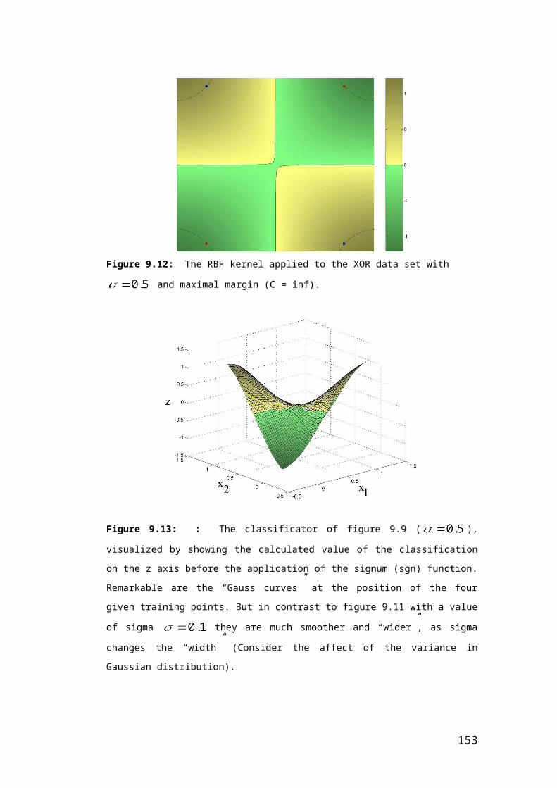
Figure C.1.2: A graphical solution to a function in 2 variables with one equality constraint

And now the solution with the Lagrangian method. As seen in chapter 4, the Lagrangian for a objective function f(x, y) in two vari-ables with one constraint g(x, y) = c is defined as:

The necessary conditions for a optimal solution can then be stated as (find stationary point(s)):

Therefore the example can be reformulated in that way:

And to find the stationary point(s):

153

This (linear) system of equalities has following solution:

x = 2, y = 1 und = 4.

So the only stationary point of f(x, y) constrained by g(x, y) is x0 = (2; 1).

Lagrangian method on a constrained function in three variables and two constraints.

We search the stationary points of the function

f(x, y, z) =

constrained by

and

Recall the generalized Lagrangian function for equality constraints in chapter 3:

for a function f of n variables and k equality constraints g i of the form .

So the Lagrangian function for the example is:

And the conditions for stationary points of L can be stated as:

And again we get a (linear) system with 5 unknowns in 5 variables, which can be easily solved and get as the only solution:

154

And so the only stationary point of f(x, y, z) with above constraints is

.

C.2 Chapter 5

Equation 5.1:

With w = , b = - 3 and x = :

Definition 5.1 (Margin): Normalisation of w and b by

w = and b = .

With w = , b = - 3:

So .

e.g:

In words normalising means scaling a vector to a length of 1, e.g.

can be seen as the diagonal in the unit quadrangle and therefore has

a length of , which is the same as . So scaling by

performs the step..

155

D SMO PSEUDO CODES

D.1 Pseudo Code of original SMO

target = desired output vectorpoint = training point matrix

procedure takeStep(i1,i2)if (i1 == i2) return 0

156

alph1 = Lagrange multiplier for i1y1 = target[i1]E1 = SVM output on point[i1] - y1 (check in error cache)m = y1*y2Compute L, H

if (L == H) return 0

k11 = kernel(point[i1],point[i1])k12 = kernel(point[i1],point[i2])k22 = kernel(point[i2],point[i2])

eta = 2*k12-k11-k22

if (eta < 0){ a2 = alph2 - y2*(E1-E2)/eta if (a2 < L) a2 = L else if (a2 > H) a2 = H}

else{ Lobj = objective function at a2=L Hobj = objective function at a2=H

if (Lobj > Hobj+eps) a2 = L

else if (Lobj < Hobj-eps) a2 = H

else a2 = alph2}

if (a2 < 1e-8) a2 = 0

else if (a2 > C-1e-8) a2 = Cif (|a2-alph2| < eps*(a2+alph2+eps)) return 0

a1 = alph1+m*(alph2-a2)

Update threshold to reflect change in Lagrange multipliersUpdate weight vector to reflect change in a1 & a2, if linear SVMUpdate error cache using new Lagrange multipliersStore a1 in the alpha arrayStore a2 in the alpha array

157

return 1endprocedure

procedure examineExample(i2)y2 = target[i2]alph2 = Lagrange multiplier for i2E2 = SVM output on point[i2] - y2 (check in error cache)r2 = E2*y2

if ((r2 < -tol && alph2 < C) || (r2 > tol && alph2 > 0)){ if (number of non-zero & non-C alpha > 1) { i1 = result of second choice heuristic if takeStep(i1,i2) return 1 }

loop over all non-zero and non-C alpha, starting at random point { i1 = identity of current alpha if takeStep(i1,i2) return 1 }

loop over all possible i1, starting at a random point { i1 = loop variable

if takeStep(i1,i2) return 1 }}return 0

endprocedure

main routine:

initialize alpha array to all zeroinitialize threshold to zeronumChanged = 0;examineAll = 1;

while (numChanged > 0 | examineAll){ numChanged = 0;

if (examineAll) loop I over all training examples numChanged += examineExample(I)

else

158

loop I over examples where alpha is not 0 & not C numChanged += examineExample(I)

if (examineAll == 1) examineAll = 0

else if (numChanged == 0) examineAll = 1}

D.2 Pseudo Code of Keerthi’s improved SMO

target = desired output vectorpoint = training point matrixfcache = cache vector for Fi values

% Note: The definition of Fi is different from the Ei in Platt’s SMO algorithm. % The Fi does not subtract any threshold.

procedure takeStep(i1, i2)

% Much of this procedure is same as in Platt’s original SMO pseudo code

if (i1 == i2) return 0

alph1 = Lagrange multiplier for i1y1 = target[i1]F1 = fcache[i1]m = y1*y2Compute L, H

If (L == H) return 0

K11 = kernel(point[i1], point[i1])K12 = kernel(point[i1], point[i2])K22 = kernel (point[i2], point[i2])eta = 2*K12-K11-K22

if (eta < 0){ a2 = alph2 – y2*(F1-F2)/eta if (a2 < L) a2 = L else if (a2 > H) a2 = H }

else{

159

Lobj = objective function at a2=L Hobj = objective function at a2=H If (Lobj > Hobj+eps) a2 = L

else if (Lobj < Hobj - eps) a2 = H

else a2 = alph2}

if ( |a2-alph2| < eps*(a2+alph2+eps) ) return 0

a1 = alph1+m*(alph2-a2)

Update weight vector to reflect change in a1 & a2, if linear SVMUpdate fcache[i] for I in I_0 using new Lagrange multipliersStore a1 and a2 in the alpha array

% The update below is simply achieved by keeping and updating infor-% mation about alpha_i being 0, C or in between them. Using this to-% gether with target[i] gives information as to which index set I be-

longs

Update I_0, I_1, I_2, I_3 and I_4

% Compute updated F values for i1 and i2 …

fcache[i1] = F1 + y1*(a1-alph1)*k11 + y2*(a2-alph2)*k12fcache[i2] = F2 + y1*(a1-alph1)*k12 + y2(a2-alph2)*k22

Compute (i_low, b_low) and (i_up, b_up) by applying equations (A) and (B) using only i1, i2 and indices in I_0

return 1

endprocedure

procedure examineExample(i2)

y2 = target[i2]alph 2 = Lagrange multiplier for i2

if (i2 is in I_0){ F2 = fcache[i2]}

else{ compute F2 = F_i2 and set fcache[i2] = F2

% Update (b_low, i_low) or (b_up, i_up) using (F2, i2) …

160

if ((i2 is in I_1 or I_2) && (F2 < b_up)) b_up = F2, i_up = i2 else if ((i2 is in I_3 or I_4) && (F2 > b_low)) b_low = F2, i_low = i2}

% Check optimality using current b_low and b_up and, if violated, find an % index i1 to do joint optimization with i2 ….

optimality = 1

if (i2 is in I_0, I_1 or I_2){ if (b_low – F2 > 2*tol) optimality = 0, i1 = i_low}

if (i2 is in I_0, I_3 or I_4){ if (F2 – b_up > 2*tol) optimality = 0, i1 = i_up}

if (optimality == 1) return 0

% For i2 in I_0 choose the better i1 …

if (i2 is in I_0){ if (b_low – F2 > F2 – b_up) i1 = i_low

else i1 = i_up}

if takeStep(i1, i2) return 1

else return 0

endprocedure

main routine for Modification 1 (same as SMO):

initialize alpha array to all zeroinitialize b_up = -1, i_up to any index of class 1initialize b_low = 1, i_low to any index of class 2set fcache[i_low] = 1 and fcache[i_up] = -1numChanged = 0;examineAll = 1;

while (numChanged > 0 | examineAll){

161

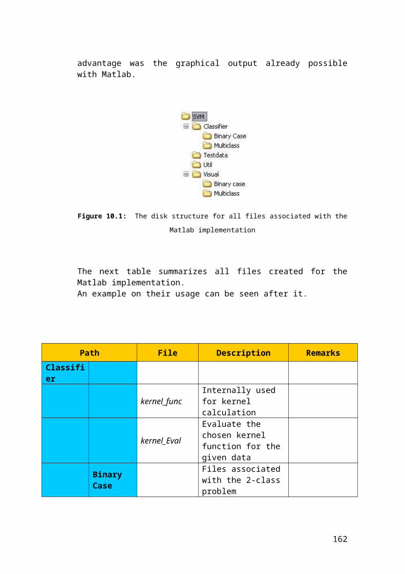
numChanged = 0;

if (examineAll) { loop I over all training examples numChanged += examineExample(I) }

else { loop I over I_0 numChanged += examineExample(I)

% It is easy to check if optimality on I_0 is attained …

if (b_up > b_low – 2*tol) at any I exit the loop after setting numChanged = 0 }

if (examineAll == 1) examineAll = 0

else if (numChanged == 0) examineAll = 1 }

main routine for Modification 2:

initialize alpha array to all zeroinitialize b_up = -1, i_up to any index of class 1initialize b_low = 1, i_low to any index of class 2set fcache[i_low] = 1 and fcache[i_up] = -1numChanged = 0;examineAll = 1;

while (numChanged > 0 | examineAll){ numChanged = 0;

if (examineAll) { loop I over all training examples numChanged += examineExample(I) }

else

% The following loop is the only difference between the two SMO modi-% fications. Whereas, in modification 1, the inner loop selects i2 from

I_0% sequentially, here i2 is always set to the current i_low and i1 is set to% the current i_up; clearly, this corresponds to choosing the worst vio-% lating pair using members of I_0 and some other indices.

162

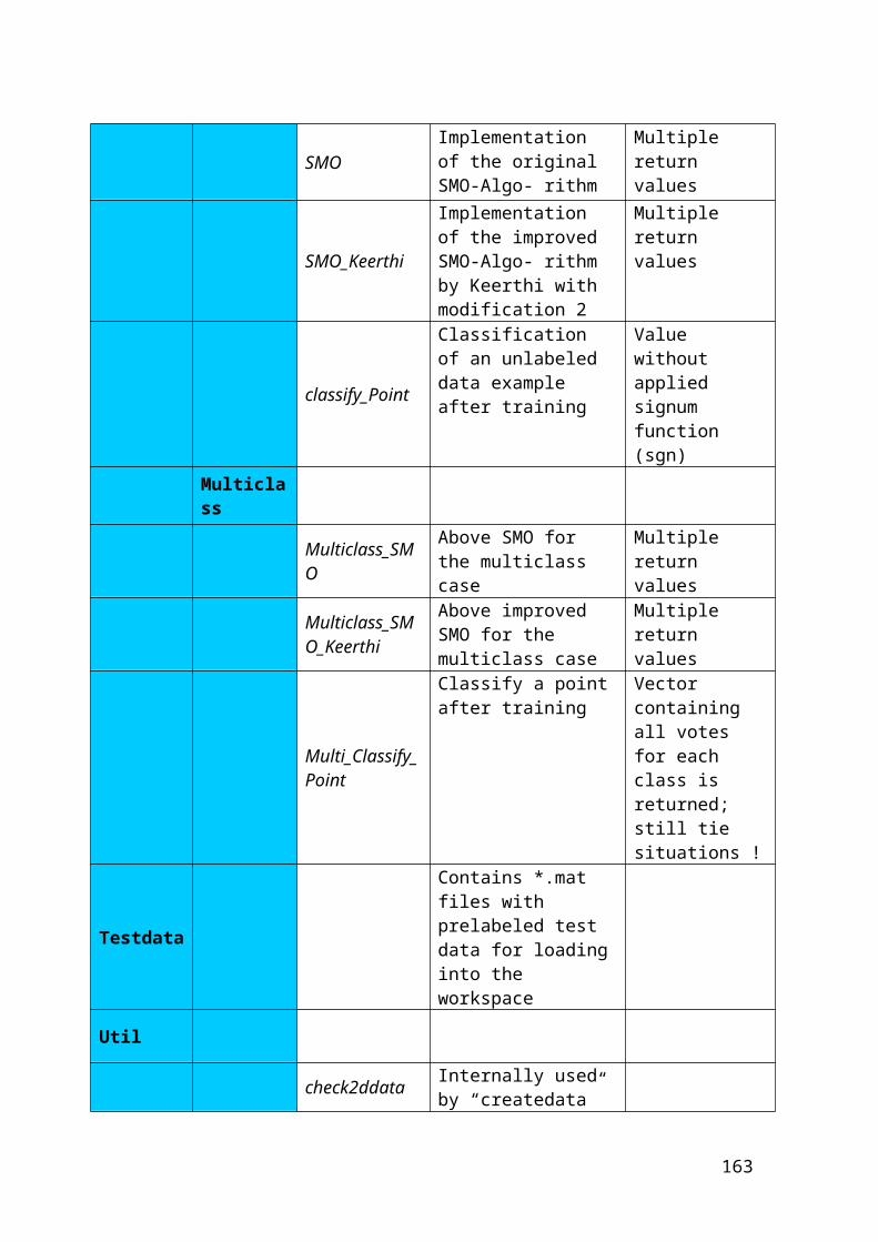
{ inner_loop_success = 1;

do until ((b_up > b_low-2*tol) | inner_loop_success == 0) { i2 = i_low y2 = target(i2) alph2 = Lagrange multiplier for i2 F2 = fcache[i2] Inner_loop_success = takeStep(i_up, i_low) numChanged += inner_loop_success }

numChanged = 0 } if (examineAll == 1) examineAll = 0

else if (numChanged == 0) examineAll = 1}

163