fábio daniel santos ferreira for multivariate analyses...manova multivariate analysis of variance...
TRANSCRIPT
Methods for Multivariate Analyses in Neuroimaging
Fábio Daniel Santos Ferreira
MASTER’S DEGREE IN BIOMEDICAL ENGINEERING
Physics Department
Faculty of Sciences and Technology of University of Coimbra
July 2014

Methods for Multivariate Analyses in Neuroimaging
Author Supervisor
Fábio D. S. Ferreira Dr. João M. Pereira
Dissertation presented to the Faculty of Sciences and Technology of the
University of Coimbra to obtain a Master’s degree in Biomedical Engineering
Coimbra, 2014


v
This thesis was developed in collaboration with:
Faculty of Medicine of the University of Coimbra
Institute for Biomedical Imaging and Life Sciences

vi

vii
Esta cópia da tese é fornecida na condição de que quem a consulta reconhece que os
direitos de autor são pertença do autor da tese e que nenhuma citação ou informação
obtida a partir dela pode ser publicada sem a referência apropriada.
This copy of the thesis has been supplied on condition that anyone who consults it is
understood to recognize that its copyright rests with its author and that no quotation
from the thesis and no information derived from it may be published without proper
acknowledgement.

viii

ix
Esta tese é dedicada aos meus pais e à minha irmã,

x
xi
Acknowledgments
Várias são as pessoas responsáveis pela conclusão deste projeto e
consequentemente pela finalização do meu Mestrado Integrado em Engenharia
Biomédica. Em primeiro lugar, e como não poderia deixar de ser, quero agradecer ao
meu orientador Dr. João Pereira por toda ajuda prestada, por todo conhecimento
transmitido, por todo o seu empenho e dedicação neste projeto e por todo o seu
profissionalismo demonstrado como orientador de uma Tese de Mestrado. Um
obrigado por tudo!
Em seguida gostaria de agradecer a mais duas pessoas que ajudaram no
aperfeiçoamento do projeto. Em primeiro lugar, ao Dr. Miguel Patrício por seguir
sempre de perto o desenvolvimento do projeto e por disponibilizar a sua ajuda sempre
que necessário. A segunda pessoa é o Investigador João Duarte por estar sempre
disponível quando era necessário e por me transmitir o seu conhecimento em Machine
Learning, nomeadamente sobre Support Vector Machines.
Quero ainda agradecer à instituição acolhedora do meu projeto, o Instituto
Biomédico de Investigação de Luz e Imagem (IBILI) da Faculdade de Medicina da
Universidade de Coimbra, por me oferecer as condições de trabalho necessárias à
realização desta dissertação. Como não poderia deixar de ser, quero também
agradecer ao Prof. Doutor Miguel Castelo-Branco, coordenador científico do IBILI, por
criar diversas possibilidades para os alunos de Engenharia Biomédica contactarem com
o mundo da investigação biomédica. Quero ainda agradecer ao Prof. Doutor Miguel
Morgado, coordenador do curso de Mestrado Integrado em Engenharia Biomédica,
por toda a dedicação que tem oferecido na organização do curso e por estar sempre
disponível para ajudar.
Por fim, os mais importantes e sempre presentes nesta minha caminhada
académica pela cidade dos amores: a família e os amigos. Em relação à família, quero
destacar os meus pais e a minha irmã por estarem sempre presentes em todos os
momentos e pelo apoio incondicional. Quanto aos amigos, quero agradecer
especialmente: à Mafalda pela sua compreensão e cumplicidade, ao Gonçalo, ao

xii
Ricardo, ao Rocha, à Adriana, ao Levita, ao Miguel, ao Diogo, ao Gil, ao Fernando e ao
Filipe por partilharem Coimbra comigo. Um obrigado a todos por tudo!
xiii
Abstract
Neuroimaging is a vast area that includes a wide range of brain-mapping
techniques, each with specific information about the brain. As each technique has its
strengths and weaknesses, it is desirable to aim for multimodal studies to possibly
obtain more relevant information. Currently, the typical strategy in neuroimaging data
analysis consists of a massive univariate approach, using the General Linear Model
(GLM) in voxel based morphometry (VBM). However, this may be insufficient to
obtain a realistic analysis due to the complexity of the structure of the brain. This leads
to the application of multivariate methods, whereby information from different
modalities can be integrated. Support Vector Machines (SVMs) and related tools are
widely used, but these do not use statistical inference tests or provide p-values for
every voxel of an image, leading to difficulties in interpretation and generalization. As
such, this thesis focuses on implementation of inferential multivariate methods that are
both a natural extension of the univariate methods commonly used and allow for the
integration of the information from different imaging modalities. Given time and data
constraints, the focus of this thesis rested on two MRI contrasts: volumetric T1
(‘Anatomy’ scans) and T2 (‘Pathology’ scans) scans obtained from 42 control and 34
type II diabetes mellitus (T2DM) subjects. This simultaneous analysis is pertinent
because it is known that T2DM leads to gray matter atrophy and vasopathies that
predispose the brain to ischemia and subcortical lacunar infarcts. All inferential
methods were implemented in Matlab and were compared with those conducted with
SPM8 software. The classification method (SVM) was performed in the PRoNTo
toolbox. Results in both univariate and multivariate analyses showed gray matter
atrophy and possible vascular changes in the limbic lobe, sub-lobar, insular and
temporal areas of the T2DM brains. Furthermore, results indicate that the multivariate
methods may lead to more specific results than the univariate ones. A toolbox was
developed to be used in the software package SPM8, where the featured methods may
be made publicly available. Despite the limitations, notably that some of the pre-
requisites to perform multivariate statistical tests were not tested, this proof of
concept shows great promise. Future work will focus on surpassing these limitations
and on preparing the methods to be applied in other multimodal (PET, fMRI) studies.

xiv
Keywords: MRI, VBM, Type II Diabetes Mellitus, Multivariate GLM
xv
Resumo
A neuroimagem é uma vasta área que inclui uma ampla gama de técnicas de
mapeamento cerebral, cada uma com informações específicas sobre o cérebro. Como
cada técnica tem os seus pontos fortes e fracos, é desejável o uso de estudos
multimodais para possivelmente obter informação mais relevante. Atualmente, a
estratégia típica na análise de dados de neuroimagem consiste numa abordagem
univariada em massa, utilizando o Modelo Linear Geral (GLM, em inglês) no VBM
(Voxel Based Morphometry). Contudo, esta abordagem pode não ser suficiente para se
obter uma análise realista devido à complexidade da estrutura cerebral. Por isto surge
a necessidade do uso de métodos multivariados, através dos quais é possível integrar
informação de diferentes modalidades. As máquinas de vetores de suporte (SVMs, em
inglês) e outras ferramentas relacionadas são amplamente usadas, no entanto estas não
usam testes de inferência estatística ou fornecem valores p para cada voxel de uma
imagem, o que leva a dificuldades de interpretação e generalização. Portanto, esta tese
foca-se na implementação de métodos multivariados inferenciais que são uma extensão
natural dos métodos univariados já usados e, para além disto, permitem a integração
de diferentes modalidades de imagem. Com as limitações de tempo e de dados, o foco
desta tese recaiu sobre dois contrastes de Imagem por Ressonância Magnética (MRI,
em inglês): T1 (scans de 'Anatomia') e T2 (scans de ‘patologia’), obtidos de 42
controlos e de 34 pacientes com diabetes tipo 2. A análise simultânea destes dois
contrastes poderá possibilitar uma melhor compreensão desta patologia, uma vez que
se sabe que a diabetes tipo 2 contribui para a atrofia da massa cinzenta e vasopatias
que predispõem o cérebro a isquemia e enfartes lacunares subcorticais. Todos os
métodos inferenciais foram implementados em Matlab e comparados com os
realizados no software SPM8. O método de classificação (SVM) foi realizado na toolbox
PRoNTo. Os resultados, tanto das análises univariadas como das multivariadas,
revelaram atrofia da massa cinzenta e possíveis alterações vasculares no lobo límbico,
sub-lobar, áreas insulares e temporais do cérebro de doentes com diabetes tipo 2.
Para além disto, os resultados indicam que os métodos multivariados podem levar a
resultados mais específicos do que os univariados. Foi ainda preparada uma toolbox
para ser usada no pacote de software SPM8, onde os métodos desenvolvidos podem
ser disponibilizados publicamente. Apesar de algumas limitações, nomeadamente que

xvi
alguns dos pré-requisitos para a realização de testes estatísticos multivariados não
foram testados, esta prova de conceito apresenta-se promissora. O trabalho futuro
focar-se-á em superar estas limitações e preparar estes métodos para outros estudos
multimodais (PET, fMRI).
Palavras-chave: MRI, VBM, Diabetes tipo 2, GLM multivariado

xvii
Symbols & Abbreviations
Symbols
Residual variance estimates
, Sample mean vectors
Variance-covariance matrix
Fitted values matrix/vector
Weight vector
Degrees of freedom
Parameters estimates matrix/vector
Chi-square
A, M A and M matrices of multivariate contrast matrix
B0 Magnetic field
C, c Contrast matrix and contrast vector
f Larmor frequency
Mg Net magnetization vector
Mgxy Transversal net magnetization vector
Mgz Longitudinal net magnetization vector
R Multiple correlation coefficient
t, F t and F statistics
T2 Hotelling’s T2
Var Variance
X Design matrix
Y Observation vector/matrix
Gyromagnetic ratio
Residual errors matrix/vector
Wilk’s lambda
B, W Sum of squares and cross products matrices between and within
λ Eigenvalues
xviii
Abbreviations
ANCOVA Analysis of Covariance
ANOVA Analysis of Variance
CSF Cerebrospinal Fluid
DV Dependent Variable
fMRI functional Magnetic Resonance Imaging
FOV Field Of View
FT Fourier Transform
FWHM Full Width at Half Maximum
GLM General Linear Model
GM Gray Matter
IV Independent Variable
LOO Leave One Out
MANCOVA Multivariate Analysis of Covariance
MANOVA Multivariate Analysis of Variance
MGLM Multivariate General Linear Model
MNI Montreal Neurological Institute
MOG Mixture of Gaussians
MPRAGE Magnetization-Prepared Rapid Gradient Echo
MRI Magnetic Resonance Imaging
PET Positron Emission Tomography
PoC Proof of Concept
PRoNTo Pattern Recognition for Neuroimaging Toolbox
RF Radiofrequency
ROI Region of Interest
SAR Specific Absorption Rate
SPACE Sampling Perfection with Application optimized Contrasts using
different flip angle Evolution
SPM Statistical Parametric Mapping
SSB Sum of Squares Between
SSCP Sum of Squares and Cross Products
SST Sum of Squares Total
SSW Sum of Squares Within
xix
SVM Support Vector Machine
T1DM Type I Diabetes Mellitus
T2DM Type 2 Diabetes Mellitus
TE Echo Time
TIV Total Intracranial Volume
TPM Tissue Probability Map
TR Repetition Time
VBM Voxel Based Morphometry
WHO World Health Organization
WM White Matter

xx
xxi
List of Figures
Figure 1.1 – Examples of T1 (right) and T2 MR (left) images. ................................................................................. 3
Figure 2.1 - (Left) The distribution of the magnetic moments of the nuclei without a magnetic field.
(Right) The distribution of the magnetic moments of the nuclei when there is a strong external magnetic
field, along with the resulting net magnetization vector [15]. ................................................................................. 7
Figure 2.2 - (A) The orientation of the spins in presence of an external magnetic field. (B) The net
magnetization vector (M) flips 90° from the longitudinal plane (the positive z-axis) to transverse x-y
plane [15]. ............................................................................................................................................................................. 8
Figure 2.3 - T1 and T2 relaxation time representation [15].................................................................................... 9
Figure 2.4 – T1 and T2 images, respectively, obtained in SPM8. .......................................................................... 11
Figure 2.5 - Spatial normalization in VBM (images obtained in SPM8). ............................................................... 13
Figure 2.6 - Segmentation in VBM (images obtained in SPM8). ............................................................................. 14
Figure 2.7 - Smoothing in VBM (images obtained in SPM8). .................................................................................. 15
Figure 3.1 - F distribution [23]....................................................................................................................................... 23
Figure 3.2 - The new design menu for the MANCOVA algorithm. ..................................................................... 30
Figure 3.3 - The new contrast window for the multivariate contrast. ................................................................ 31
Figure 3.4 - The general process of classification algorithms [31]. ...................................................................... 32
Figure 3.5 - Illustration of the SVM concept in an imaginary 2D space [4]........................................................ 34
Figure 4.1 - An example of overlapping a (blue) significance map image with a high resolution image. ..... 37
Figure 4.2 - ANCOVA obtained with an in-house function in Matlab, using T1 images. ............................... 39
Figure 4.3 – The previous ANCOVA image overlaid with a high resolution image. ....................................... 39
Figure 4.4 - ANCOVA obtained in SPM8 (VBM), using T1 images. ..................................................................... 40
Figure 4.5 - ANCOVA obtained with an in-house function in Matlab, using T2 images. ............................... 41
Figure 4.6 - The previous ANCOVA image overlaid with a high resolution image. ....................................... 41
Figure 4.7 - ANCOVA obtained in SPM8 (VBM), using T2 images. ..................................................................... 42
Figure 4.8 - ANOVA, with concatenation of T1 and T2 images, obtained with an in-house function in
Matlab. .................................................................................................................................................................................. 43
Figure 4.9 - ANOVA, with concatenation of T1 and T2 images, image overlaid with a high resolution
image. ................................................................................................................................................................................... 43
Figure 4.10 - ANOVA, with concatenation of T1 and T2 images, obtained in SPM8 (VBM). ....................... 44
Figure 4.11 - ANCOVA, with concatenation of T1 and T2 images, obtained with an in-house function in
Matlab. .................................................................................................................................................................................. 45
xxii
Figure 4.12 - ANCOVA image, with concatenation of T1 and T2 images, overlaid with a high resolution
image. ................................................................................................................................................................................... 45
Figure 4.13 - ANCOVA, with concatenation of T1 and T2 images, obtained in SPM8 (VBM). .................... 46
Figure 4.14 - Two-sample Hotelling's T2 obtained with an in-house function in Matlab. ............................... 48
Figure 4.15 - The previous Hotelling's T2 image overlaid with a high resolution image. ................................ 48
Figure 4.16 - MANOVA obtained with an in-house function in Matlab. ............................................................ 49
Figure 4.17 - The previous MANOVA image overlaid with a high resolution image. ..................................... 49
Figure 4.18 - MANCOVA obtained with an in-house function in Matlab. ......................................................... 50
Figure 4.19 - The previous MANCOVA image overlaid with a high resolution image. .................................. 51
Figure 4.20 - MANCOVA obtained in SPM8 (VBM). ............................................................................................... 51
Figure 4.21 – The results of the inferential multivariate methods (A - Hotelling’s T2, B - MANOVA and C
- MANCOVA), compared with a map of weights, obtained in PRoNTo software using SVM algorithm
(D), at the coordinate [-10.7 15.4 1.7] mm. .............................................................................................................. 52
xxiii
Contents
Acknowledgments ......................................................................................................... xi
Abstract ........................................................................................................................ xiii
Resumo ........................................................................................................................... xv
Symbols & Abbreviations ............................................................................................ xvii
List of Figures ............................................................................................................... xxi
Contents ..................................................................................................................... xxiii
CHAPTER 1 .......................................................................................................... 1
Introduction ..................................................................................................................... 1
CHAPTER 2 .......................................................................................................... 5
Structural brain imaging of type 2 diabetes ................................................................. 5
2.1 Type 2 diabetes mellitus ........................................................................................................... 5
2.2 Magnetic Resonance Imaging .................................................................................................. 6
2.2.1 The formation of the MR Signal ...................................................................................... 6 2.2.2 Image Formation (Spatial Encoding) ............................................................................... 9 2.2.3 Tissue Contrast ............................................................................................................... 10
2.3 Voxel Based Morphometry (VBM) ........................................................................................ 11
2.3.1 Spatial Normalization/Registration .............................................................................. 12 2.3.2 Segmentation and Modulation ...................................................................................... 13 2.3.3 Smoothing ......................................................................................................................... 15 2.3.4 Statistical Analysis ............................................................................................................ 15
CHAPTER 3 ........................................................................................................ 17
Statistics ......................................................................................................................... 17
3.1 Univariate Statistics .................................................................................................................. 17
3.1.1 Univariate GLM ................................................................................................................ 17 3.1.1.1 Contrasts ...................................................................................................................................... 20 3.1.1.2 T-test ............................................................................................................................................. 20
3.1.2 Implemented Methods ................................................................................................... 22 3.1.2.1 Analysis of Variance / F-test .................................................................................................... 22 3.1.2.2 Analysis of Covariance .............................................................................................................. 24
3.2 Multivariate Statistics ............................................................................................................... 25
3.2.1 Multivariate GLM ............................................................................................................. 25 3.2.1.1 Multivariate GLM Representation and Parameter Estimation ........................................ 25 3.2.1.2 Testing the Multivariate General Linear Hypothesis ........................................................ 26
3.2.2 Implemented Methods ................................................................................................... 28 3.2.2.1 Hotelling’s T2 ............................................................................................................................... 28 3.2.2.2 Multivariate Analysis of Variance ........................................................................................... 28 3.2.2.3 Multivariate Analysis of Covariance ...................................................................................... 29 3.2.2.4 Alterations in SPM8 interface ................................................................................................. 29
3.3 Support Vector Machine.......................................................................................................... 32
xxiv
CHAPTER 4 ........................................................................................................ 35
Implementation ............................................................................................................ 35
4.1 Methods ....................................................................................................................................... 35
4.1.1 Patient Selection .............................................................................................................. 35 4.1.2 Image Acquisition ............................................................................................................ 35 4.1.3 SPM Analyses .................................................................................................................... 36 4.1.4 Image analyses outside SPM .......................................................................................... 36 4.1.5 Overlap of results with a high resolution image ...................................................... 36 4.1.6 Pattern Recognition for Neuroimaging Toolbox ..................................................... 37
4.2 Results .......................................................................................................................................... 38
4.2.1 Univariate Analyses ......................................................................................................... 38 4.2.1.1 ANCOVA ..................................................................................................................................... 38
4.2.1.1.1 T1 images ............................................................................................................................................... 39 4.2.1.1.2 T2 images ............................................................................................................................................... 41
4.2.1.2 ANOVA with concatenation of T1 and T2 images ........................................................... 42 4.2.1.3 ANCOVA with concatenation of T1 and T2 images ........................................................ 44
4.2.2 Multivariate Analyses ...................................................................................................... 47 4.2.2.1 Inferential Methods .................................................................................................................... 47
4.2.2.1.1 Hotelling’s T2 ......................................................................................................................................... 47 4.2.2.1.2 MANOVA .............................................................................................................................................. 48 4.2.2.1.3 MANCOVA ........................................................................................................................................... 49
4.2.2.2 Classification/Pattern Recognition Methods ....................................................................... 52
CHAPTER 5 ........................................................................................................ 53
Discussion & Conclusions ............................................................................................. 53
5.1 Univariate Analyses and Type 2 Diabetes Mellitus .......................................................... 53
5.2 Multivariate Analyses and Type 2 Diabetes Mellitus ....................................................... 54
5.3 Possible Future SPM8 toolbox ................................................................................................ 55
5.4 Limitations & Future work ...................................................................................................... 56
References ..................................................................................................................... 57
Annex A. Tutorial for SPM8 alterations ..................................................................... 61
Chapter 1 – Introduction 1
Chapter 1
Introduction
Neuroimaging is a vast field that covers a wide range of brain-mapping
techniques, each with specific information about the brain. Broadly, magnetic
resonance imaging (MRI) is used for structural analyses, functional MRI (fMRI) for
functional analyses, and positron emission tomography (PET) for metabolic and
neurochemical analyses. Each modality has its strengths and weaknesses, and the
information that each can provide is complementary when building to the broad array
of scientific hypotheses in the field. As such, it is desirable to aim for multimodal
studies, i.e. studies in which several imaging modalities are combined: with the
integration of imaging techniques, more information may be obtained, reaching beyond
the scope of any individual method [1].
At its most basic, neuroimaging analyses proceed by localizing brain regions that
exhibit experimental variation, either correlative with a covariable or comparative
between groups. In brain morphometry, where the goal is to study changes in the
shape and volume of brain structures (e.g. atrophy in dementia), the typical strategy
consists of a massive univariate approach where the statistical model is performed on a
voxel-by-voxel basis: the result is a 3D statistical map that can be used to infer on the
presence of an effect at each voxel [2]. The statistical models usually used are based on
linear models, notably ANOVA/ANCOVA (Analysis of Variance/Covariance),
correlation coefficients and t-tests. All of these are specials cases of the General Linear
Model (GLM), which lies at the basis of the statistical parametric maps hypothesis
testing on regionally specific effects in neuroimaging data [3].
Chapter 1 – Introduction 2
Although these univariate methods have been fundamental tools in modern
neuroimaging, by aiding in the detection of group differences and in the understanding
of spatial patterns of functional activation, the presence of multivariate relationships
between different brain regions may not be explained by univariate analyses alone. This
leads to the application of multivariate methods, whereby multiple imaging modalities
can be analyzed simultaneously, eventually leading to a better understanding of imaging
profiles of brain activity, structure and pathology. A common example of this recent
trend is the support vector machines (SVMs) and related tools [4]. These supervised
machine learning methods are useful in identifying features that aid in group/pathology
classification [5]. Nonetheless, SVMs do not use statistical inference tests or provide p-
values for every voxel of an image, leading to difficulties in interpretation and
generalization [4]. Instead, SVMs determine a ‘weight coefficient’ for every voxel of an
image, the distribution of which does not have a clear analytic interpretation [6].
Bypassing the limitations seen in SVMs, and focusing solely on inferential
analyses rather than pattern recognition, this thesis presents multivariate methods that
are a natural extension of the massive univariate approach commonly used, allowing
for the integration of different imaging modalities such as fMRI, PET and MRI. Given
time and data constraints, the focus will lie on two MRI contrasts: volumetric T1 and
T2 scans obtained from subjects who participated in the Diamarker project.
The Diamarker project aims to evaluate the genetic susceptibility of multi-
systemic complications of type II diabetes mellitus (T2DM) in order to identify new
biomarkers for diagnosis and therapeutic monitoring. One of the tasks, where this
thesis fits in, is related to the structural and functional analyses of the brain through
MRI scanning. The project is built around a consortium, which includes the Faculty of
Medicine of the University of Coimbra, the University Hospital of Coimbra, IBILI,
IEETA/UA, as well as members of the industry, notably Siemens.
T2DM is known to be characterized by early onset endothelial dysfunction and
vascular damage [7], cognitive decline [7-11] and emotional alterations [11], as well as
brain structural and functional alterations [8, 9]. This thesis will focus on brain
structure and vascular alterations: it is known that T2DM leads to gray matter (GM)

Chapter 1 – Introduction 3
atrophy [7-11] and vasopathies that predispose the brain to ischemia and subcortical
lacunar infarcts [7-11]. In order to extract information about both GM atrophy and
vascular alterations, it is necessary to acquire both T1 and T2 magnetic resonance
(MR) images. It is important to underline that, although both types of image can
provide structural information of the brain, T1 images (‘Anatomic’ scans) have better
contrast than T2 images and so better anatomic information. However, T2 images
(‘Pathology’ scans) provide a better examination of the brain vasculature [12].
Therefore, the integration of T1 and T2 MR images, in order to obtain more
information, is a sensible approach.
Figure 1.1 – Examples of T1 (right) and T2 MR (left) images.
Hereupon, the main goals of this thesis are as follows:
1) Replicate the univariate VBM analyses between controls and T2DM
patients, using SPM8 software (Statistical Parametric Mapping,
http://www.fil.ion.ucl.ac.uk/spm/software/spm8/) as a reference;
2) Explore and implement multivariate methods that can integrate
information from T1 (structural information) and T2 (structural +
vascular information) MR images – each type of image can be seen as
a Dependent Variable (DV) – contrasting controls to T2DM patients
(Independent Variables, IVs);

Chapter 1 – Introduction 4
3) Insertion of these algorithms into the pipeline of SPM8 in order for it
to be used in further multimodal studies.
Chapter 2 – Structural brain imaging of type 2 diabetes 5
Chapter 2
Structural brain imaging of type 2 diabetes
2.1 Type 2 diabetes mellitus
Diabetes mellitus is a chronic metabolic disease characterized by a disorder of
the carbohydrate metabolism, which can be divided in two major types: type 1 and
type 2 diabetes mellitus, T1DM and T2DM, respectively. T1DM appears mainly in
children [7] and results from dysfunction in insulin-producing pancreatic cells,
possibly due to inadequate autoimmune destruction, leading to low insulin release - it
is also known as insulin-dependent diabetes mellitus [7, 8]. T2DM appears mostly in
adults and represents about 90% of all diabetes cases [7]. It presents itself as an
insensitivity to insulin, and is also known as non-insulin-dependent diabetes mellitus.
This latter presentation of diabetes has been linked to obesity, as well as to other co-
morbidities, known together as the metabolic syndrome [7, 8]. Both of types of
diabetes lead to hyperglycaemia if uncontrolled.
In the literature, it is well accepted that diabetes may potentiate microvascular
lesions (as linked to nephropathy and retinopathy) as well as macrovascular lesions
(arteriosclerosis and cardiovascular disease). Furthermore, both T1DM and T2DM can
induce both peripheral (neuropathy) and central nervous system (CNS) complications
[7]. This thesis will only focus on brain alterations caused by T2DM.
T2DM is known to be characterized by early onset endothelial dysfunction and
vascular damage [7], cognitive decline [7-11] and emotional alterations [11], as well as
brain structural and functional alterations [8, 9]. Furthermore it is known that T2DM

Chapter 2 – Structural brain imaging of type 2 diabetes 6
leads to GM atrophy [7-11] and vasopathies that predispose the brain to ischemia and
subcortical lacunar infarcts [7-11]. These brain abnormalities, particularly in the elderly,
have also been associated with the increased risk for dementia [9].
It is the most prevalent metabolic chronic disease worldwide (by 2030, 82
million of elderly over 64 years of age are projected to have T2DM in developing
countries and over 48 million in developed countries) [7]. Consequently, it is both
relevant and urgent to better understand the impact of this pathology in the brain.
2.2 Magnetic Resonance Imaging
Magnetic Resonance Imaging is a diagnostic imaging technique that uses a
combination of strong magnetic fields, radiofrequency signals and dedicated equipment
including a powerful computer to create pictures of internal body structures [13].
2.2.1 The formation of the MR Signal
Biological tissues are composed of atoms, such as hydrogen, carbon, sodium
and phosphorus, which have magnetic properties that make them inherently
susceptible to a magnetic field. As the hydrogen nuclei are the most abundant in any
biological system, clinical MRI is focuses on these nuclei - in essence single protons - in
both water and macromolecules, such as proteins and fat [14].
Sub-atomic particles and protons in particular, have a quantum property known
as spin: in a classical sense, protons can be pictured as spinning around their axes, thus
behaving like small magnetic dipoles. The magnetic momentum generated, under
standard thermal circumstances, has a random spatial orientation: globally, within a
tissue, the individual nuclei magnetic moments cancel each other out, leading to a null
net magnetization vector (Mg) [14, 15] (Figure 2.1). In the presence of a strong
external magnetic field, however, they become aligned with this field and can adopt
two possible orientations: parallel (lower energy state) or antiparallel (higher energy
state) to the magnetic field. As the parallel is the preferred alignment, the result is a
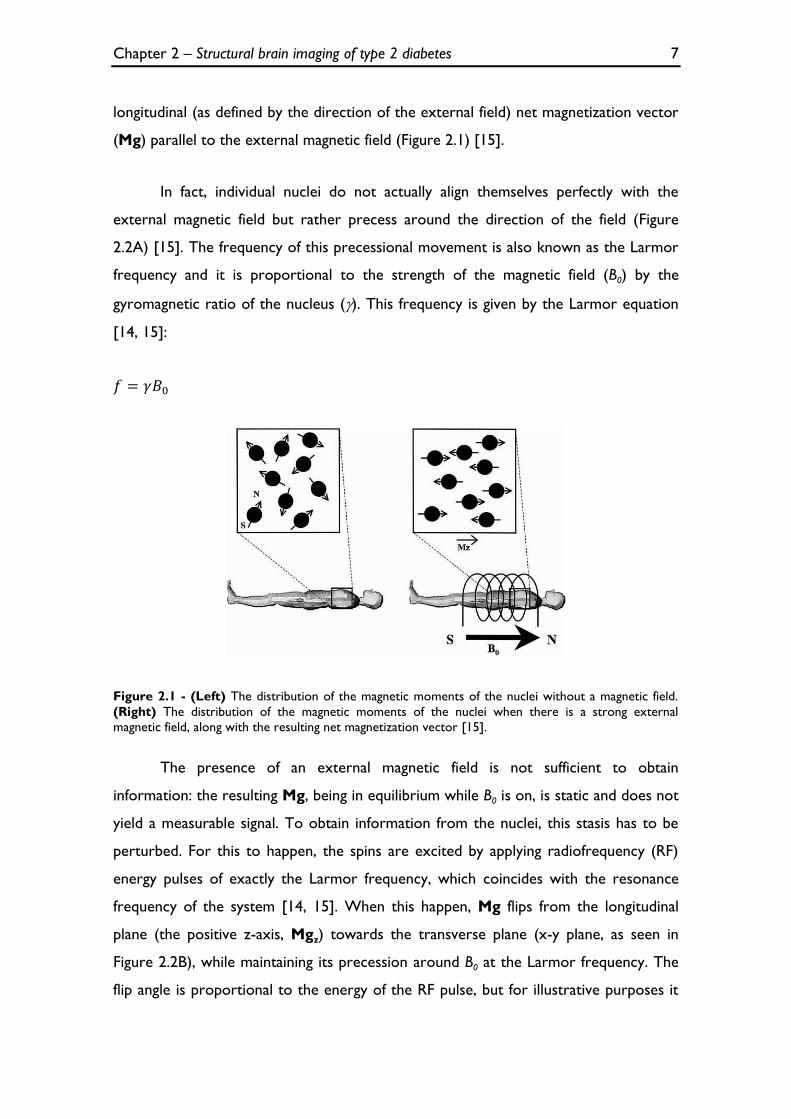
Chapter 2 – Structural brain imaging of type 2 diabetes 7
longitudinal (as defined by the direction of the external field) net magnetization vector
(Mg) parallel to the external magnetic field (Figure 2.1) [15].
In fact, individual nuclei do not actually align themselves perfectly with the
external magnetic field but rather precess around the direction of the field (Figure
2.2A) [15]. The frequency of this precessional movement is also known as the Larmor
frequency and it is proportional to the strength of the magnetic field (B0) by the
gyromagnetic ratio of the nucleus (). This frequency is given by the Larmor equation
[14, 15]:
Figure 2.1 - (Left) The distribution of the magnetic moments of the nuclei without a magnetic field.
(Right) The distribution of the magnetic moments of the nuclei when there is a strong external
magnetic field, along with the resulting net magnetization vector [15].
The presence of an external magnetic field is not sufficient to obtain
information: the resulting Mg, being in equilibrium while B0 is on, is static and does not
yield a measurable signal. To obtain information from the nuclei, this stasis has to be
perturbed. For this to happen, the spins are excited by applying radiofrequency (RF)
energy pulses of exactly the Larmor frequency, which coincides with the resonance
frequency of the system [14, 15]. When this happen, Mg flips from the longitudinal
plane (the positive z-axis, Mgz) towards the transverse plane (x-y plane, as seen in
Figure 2.2B), while maintaining its precession around B0 at the Larmor frequency. The
flip angle is proportional to the energy of the RF pulse, but for illustrative purposes it
Chapter 2 – Structural brain imaging of type 2 diabetes 8
will be assumed to be 90º: in this situation, the magnetization becomes fully transversal
(Mgxy). When placing a receiver coil along the x or y axis (in practice, two coils are
used in quadrature), this rotation will induce an alternating current that can be
measured by a receiver coil – this signal is called free induction decay (FID), for
reasons that will become apparent below [15].
Figure 2.2 - (A) The orientation of the spins in presence of an external magnetic field. (B) The net
magnetization vector (M) flips 90° from the longitudinal plane (the positive z-axis) to transverse x-y
plane [15].
The longitudinal relaxation, directly linked to the process of realignment to the
external magnetic field, also known as spin-lattice relaxation, is characterized by the T1
relaxation (decay) time. This is defined as the time required for the system to recover
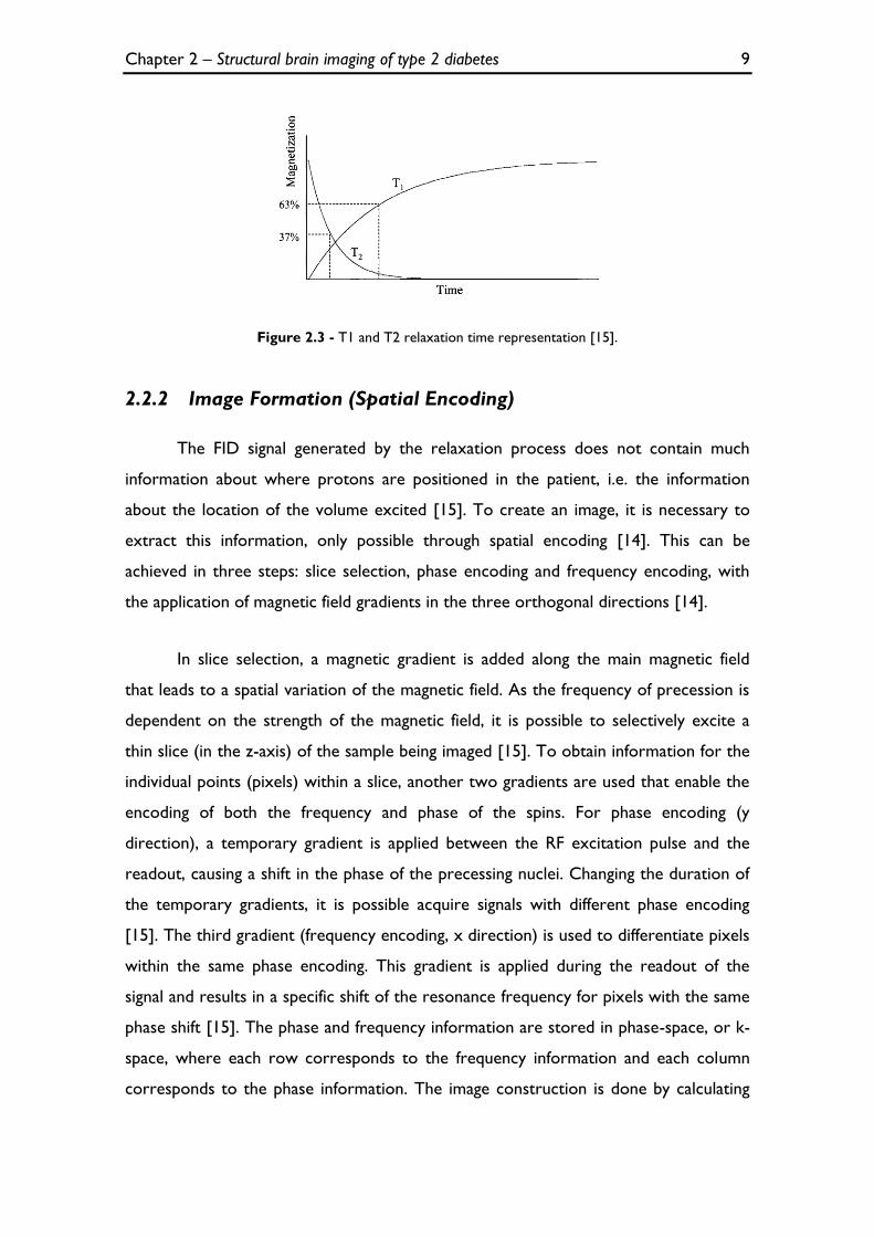
to 63% of its equilibrium value after it has been exposed to a RF pulse (Figure 2.3) [14,
15]. It occurs due to the energy losses between the spin of any given nucleus and the
surrounding atomic lattice, hence the name. The transverse relaxation, or spin-spin
relaxation, is caused by the loss of the phase coherence amongst the precessing H-
protons in the transverse plane and is characterized by T2 relaxation time. This
corresponds to the time it takes to the signal to decay to 37% of its original value
(Figure 2.3) [14, 15]. Biological tissues have different T1 and T2 values, but the T2 time
is always shorter than the T1 time: this is the fundamental basis of MRI soft tissue
contrast.
Chapter 2 – Structural brain imaging of type 2 diabetes 9
Figure 2.3 - T1 and T2 relaxation time representation [15].
2.2.2 Image Formation (Spatial Encoding)
The FID signal generated by the relaxation process does not contain much
information about where protons are positioned in the patient, i.e. the information
about the location of the volume excited [15]. To create an image, it is necessary to
extract this information, only possible through spatial encoding [14]. This can be
achieved in three steps: slice selection, phase encoding and frequency encoding, with
the application of magnetic field gradients in the three orthogonal directions [14].
In slice selection, a magnetic gradient is added along the main magnetic field
that leads to a spatial variation of the magnetic field. As the frequency of precession is
dependent on the strength of the magnetic field, it is possible to selectively excite a
thin slice (in the z-axis) of the sample being imaged [15]. To obtain information for the
individual points (pixels) within a slice, another two gradients are used that enable the
encoding of both the frequency and phase of the spins. For phase encoding (y
direction), a temporary gradient is applied between the RF excitation pulse and the
readout, causing a shift in the phase of the precessing nuclei. Changing the duration of
the temporary gradients, it is possible acquire signals with different phase encoding
[15]. The third gradient (frequency encoding, x direction) is used to differentiate pixels
within the same phase encoding. This gradient is applied during the readout of the
signal and results in a specific shift of the resonance frequency for pixels with the same
phase shift [15]. The phase and frequency information are stored in phase-space, or k-
space, where each row corresponds to the frequency information and each column
corresponds to the phase information. The image construction is done by calculating
Chapter 2 – Structural brain imaging of type 2 diabetes 10
the 2D (or 3D, if pure three dimensional acquisition) inverse Fourier Transform (FT)
of the samples gathered in k-space.
2.2.3 Tissue Contrast
The differences in proton density over the different tissues provide a basic form
of MR imaging contrast, i.e. there are organs with low proton density (e.g. lungs) that
contrast with organs with high proton density (e.g. heart muscle) [14]. However, there
are other ways to discern differences between tissues, which imply the construction of
imaging sequences of RF pulses that allow for the visualization of the difference in T1
and T2 time constants. It is therefore fundamental to tune two important parameters
of pulses sequences: the time between two consecutive RF pulses, known as repetition
time (TR), and the time between two consecutive RF pulses and echo, known as echo
time (TE). For short TR and TE, the contrast in the image will be potentiated by the
difference in T1 value of the tissues (T1-weighted sequences or T1 images). On the
other hand, using long TR and TE, the contrast will be dependent on T2 differences
(T2-weighted sequences or T2 images) [15].
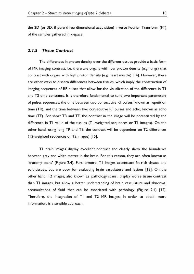
T1 brain images display excellent contrast and clearly show the boundaries
between gray and white matter in the brain. For this reason, they are often known as
‘anatomy scans’ (Figure 2.4). Furthermore, T1 images accentuate fat-rich tissues and
soft tissues, but are poor for evaluating brain vasculature and lesions [12]. On the
other hand, T2 images, also known as ‘pathology scans’, display worse tissue contrast
than T1 images, but allow a better understanding of brain vasculature and abnormal
accumulations of fluid that can be associated with pathology (Figure 2.4) [12].
Therefore, the integration of T1 and T2 MR images, in order to obtain more
information, is a sensible approach.
Chapter 2 – Structural brain imaging of type 2 diabetes 11
Figure 2.4 – T1 and T2 images, respectively, obtained in SPM8.
2.3 Voxel Based Morphometry (VBM)
A number of pathologies, such as diabetes type 2, implicate subtle changes in
shape and local volume of the brain [16]. The assessment of these can be made using
structural MRI images and measuring the volume of certain brain regions, called
regions of interest (ROIs). This method, however, fails to assess the overall brain
structure and, by design, presents regional bias. Besides, it is time consuming when
performed manually (the gold standard), and may be prone to errors. An alternative,
or at least a first port of call, is to use whole brain automated morphometry methods.
The most common of these methods is Voxel Based Morphometry (VBM), which
allows for the localization of regions of volumetric differences in brain tissue, notably in
GM [17]. VBM implies the voxel-wise analysis of local tissue volumes within a group or
across groups: the final result is a map of statistically significant alterations in tissue
volume, between groups or correlated with a given metric [16, 17]. For this, the data
are pre-processed in three steps in order to sensitize the tests to regional tissue
volumes: spatial normalization, segmentation and smoothing. After that, a statistical
analysis is performed to localize significant alterations in volume [16, 17].
Chapter 2 – Structural brain imaging of type 2 diabetes 12
2.3.1 Spatial Normalization/Registration
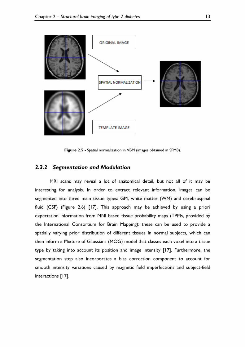
Spatial normalization consists in matching MR images and a suitable template
(Figure 2.5), by removing both global and local structural differences between brains.
This process ensures that all results are reported in standard stereotactic space (the
current standard being the MNI - Montreal Neurological Institute - space), allowing the
analysis of the voxels in a coordinate consistent manner [16]. This can be achieved in
two main steps. The first step removes global differences between subject and
template; this involves matching the MR images to the template by (linearly) estimating
the optimal 12-paremeter affine transformation (three translations, three rotations,
three scales and three for shearing) [16, 17]. The second step corresponds to a
nonlinear registration that accounts for local nonlinear shape differences, which may be
modelled by linear combination of low-frequency periodic basis functions [16, 17]. The
nonlinear registration minimizes a cost function between the MR image and the
template and, simultaneously, maximizes the smoothness of the deformations [16].
Spatial normalization attempts to match every cortical feature exactly, but that
is not possible due to anatomical variability. However, it can achieve very close
matches, which can be enough to remove key differences between subjects and the
template. If this happens, no significant differences will be detected by VBM. In order
to prevent this, the amount of local volume change is registered by calculating the
voxel-wise determinant of the Jacobian of the deformation field. This is then multiplied
to the segmentation output, as seen in the next section.
Chapter 2 – Structural brain imaging of type 2 diabetes 13
Figure 2.5 - Spatial normalization in VBM (images obtained in SPM8).
2.3.2 Segmentation and Modulation
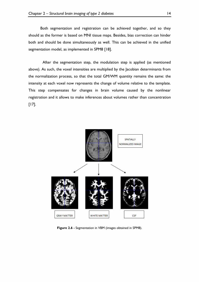
MRI scans may reveal a lot of anatomical detail, but not all of it may be
interesting for analysis. In order to extract relevant information, images can be
segmented into three main tissue types: GM, white matter (WM) and cerebrospinal
fluid (CSF) (Figure 2.6) [17]. This approach may be achieved by using a priori
expectation information from MNI based tissue probability maps (TPMs, provided by
the International Consortium for Brain Mapping): these can be used to provide a
spatially varying prior distribution of different tissues in normal subjects, which can
then inform a Mixture of Gaussians (MOG) model that classes each voxel into a tissue
type by taking into account its position and image intensity [17]. Furthermore, the
segmentation step also incorporates a bias correction component to account for
smooth intensity variations caused by magnetic field imperfections and subject-field
interactions [17].
Chapter 2 – Structural brain imaging of type 2 diabetes 14
Both segmentation and registration can be achieved together, and so they
should as the former is based on MNI tissue maps. Besides, bias correction can hinder
both and should be done simultaneously as well. This can be achieved in the unified
segmentation model, as implemented in SPM8 [18].
After the segmentation step, the modulation step is applied (as mentioned
above). As such, the voxel intensities are multiplied by the Jacobian determinants from
the normalization process, so that the total GM/WM quantity remains the same: the
intensity at each voxel now represents the change of volume relative to the template.
This step compensates for changes in brain volume caused by the nonlinear
registration and it allows to make inferences about volumes rather than concentration
[17].
Figure 2.6 - Segmentation in VBM (images obtained in SPM8).
Chapter 2 – Structural brain imaging of type 2 diabetes 15
2.3.3 Smoothing
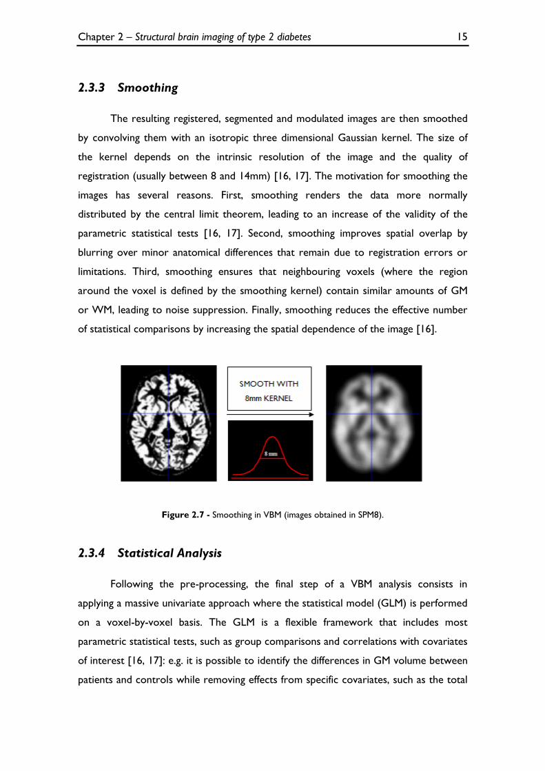
The resulting registered, segmented and modulated images are then smoothed
by convolving them with an isotropic three dimensional Gaussian kernel. The size of
the kernel depends on the intrinsic resolution of the image and the quality of
registration (usually between 8 and 14mm) [16, 17]. The motivation for smoothing the
images has several reasons. First, smoothing renders the data more normally
distributed by the central limit theorem, leading to an increase of the validity of the
parametric statistical tests [16, 17]. Second, smoothing improves spatial overlap by
blurring over minor anatomical differences that remain due to registration errors or
limitations. Third, smoothing ensures that neighbouring voxels (where the region
around the voxel is defined by the smoothing kernel) contain similar amounts of GM
or WM, leading to noise suppression. Finally, smoothing reduces the effective number
of statistical comparisons by increasing the spatial dependence of the image [16].
Figure 2.7 - Smoothing in VBM (images obtained in SPM8).
2.3.4 Statistical Analysis
Following the pre-processing, the final step of a VBM analysis consists in
applying a massive univariate approach where the statistical model (GLM) is performed
on a voxel-by-voxel basis. The GLM is a flexible framework that includes most
parametric statistical tests, such as group comparisons and correlations with covariates
of interest [16, 17]: e.g. it is possible to identify the differences in GM volume between
patients and controls while removing effects from specific covariates, such as the total

Chapter 2 – Structural brain imaging of type 2 diabetes 16
intracranial volume - TIV. The standard statistical tests used are thus parametric (t
tests and F tests, the validity of which ensured by the smoothing step as explained
above), allowing for voxel-wise hypotheses testing [16, 17]. If the pre-processing and
the choice of the statistical model are correct, after fitting the model, the resulting
residuals should be independent and normally distributed. As the statistical parametric
map generated comprises the result of many voxel-wise statistical tests, correction for
multiple comparisons is usually required when assessing the significance of an effect in
any given voxel [16, 17]. The statistics that are implicated in this final step of VBM will
be further explained in the next chapter.
Chapter 3 – Statistics 17
Chapter 3
Statistics
3.1 Univariate Statistics
In inferential statistics, one intends to explain a variable - said dependent -
based on the influence of another variable or other variables, said independent, in a
way that can be generalized to the population, starting off with a sample.
When only one dependent variable is at stake, then this analysis is designated as
univariate: this is by far the most common statistical approach given the simplicity of
the methods involved and their ease of implementation. Nonetheless, such an
approach may miss important information stored in the structure of the data, which
may not be reducible to a single dependent variable. It is, however, important to
explain the basis of key univariate tests, such as t tests, F tests, ANOVA and
ANCOVA, as these are the building blocks of more complex approaches. These simple
tests allow for the testing of the null hypothesis (i.e. absence of effect) of one or more
independent variables relating to one dependent variable [3]. As these tests are all
special cases of GLM, it is pertinent explain the mathematics and algebra that are used
in this unifying framework.
3.1.1 Univariate GLM
A basic linear regression explains a dependent continuous variable y by the
behaviour of a single independent continuous variable x, modelled by the line equation
as seen in 3.1:
Chapter 3 – Statistics 18
3.1
where is the intersect, is a regressor that represents the slope of the line,
and is the residual error of the model. The regressor is positive if the relation
between x and y is direct, and negative if inverse. Importantly, there is a p-value
attached to the regressor, the null hypothesis of which is that there is no relation
between y and x.
This basic model can be expanded in order to include more independent
variables, either continuous (covariates) or categorical (factors), each with its own
regressor, the interpretation of which is very similar to what was described for the
basic linear regression. This extension is called the general linear model.
The GLM facilitates a wide range of hypothesis testing with statistical
parametric maps [19]. When formulating a linear model, one observes a phenomenon
represented by an observed data vector (response or dependent variable), which can
be related to a set of linearly independent fixed variables (predictor or independent
variables): together they form the explanatory model being tested [2, 19].
To construct a general linear model, in presence of univariate data, an
observation vector , where N is the number of the observations, is related to k
unknown parameters, where k is the number of the predictor variables, represented
by a vector through a known design matrix . Simply put, each observation
can be described as a linear combination of independent factors and/or covariates that
influence the outcome. As with any model, an error term must be included to absorb
the unexplained variance of the system: as such, an error vector , where each
element is independent and generated by identically distributed normal random
variables, is added to the model [19, 20]:
3.2
Chapter 3 – Statistics 19
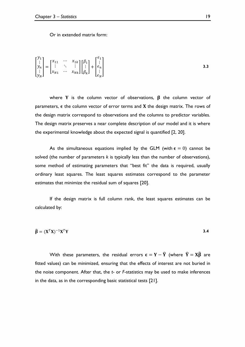
Or in extended matrix form:
3.3
where is the column vector of observations, the column vector of
parameters, the column vector of error terms and the design matrix. The rows of
the design matrix correspond to observations and the columns to predictor variables.
The design matrix preserves a near complete description of our model and it is where
the experimental knowledge about the expected signal is quantified [2, 20].
As the simultaneous equations implied by the GLM (with ) cannot be
solved (the number of parameters k is typically less than the number of observations),
some method of estimating parameters that “best fit” the data is required, usually
ordinary least squares. The least squares estimates correspond to the parameter
estimates that minimize the residual sum of squares [20].
If the design matrix is full column rank, the least squares estimates can be
calculated by:
3.4
With these parameters, the residual errors (where are
fitted values) can be minimized, ensuring that the effects of interest are not buried in
the noise component. After that, the t- or F-statistics may be used to make inferences
in the data, as in the corresponding basic statistical tests [21].
Chapter 3 – Statistics 20
3.1.1.1 Contrasts
One of the great advantages of the GLM is the use of contrasts for inference
about regressors. Contrasts are vectors (if t-contrasts) or matrices (F-contrasts) that
can be used to focus the inferential analysis on a subset of regressors, defining the
relationship between them, while possibly ignoring others. The ignored independent
variables are seen as nuisance variables, i.e. their effects are accounted for but
removed from the analysis.
As a simple example, with the GM volume as the dependent variable and 4
independent regressors -1 to-, corresponding to the independent variables related
to, e.g. T1 brain images: control, disease, TIV and age, respectively, a t-contrast = [1 -1
0 0] can be used to find the brain regions where there are more GM volume in control
subjects than disease subjects, excluding from the analysis the nuisance variables TIV
and age.
Another type of contrast that may be used is the F-contrast. While a t-contrast
tests a single linear constraint, the F-contrast is used to test whether any of several
linear constraints is true, i.e. can be seen as an OR statement containing several t-
contrasts. Using from the example above the same regressors, but different
independent variables, as follows: T1 brain images of control subjects, T1 brain images
of subjects with a disease, T2 brain images of control subjects, T2 brain images of
subjects with a disease and the same nuisance variables TIV and age, a F-contrast =
can be used to find any brain region, in T1 or T2 images, where
GM atrophy is present, excluding from the analysis the nuisance variables TIV and age.
The dependent variable remains a vector, but now it is the concatenation of the GM
values of T1 and T2 images (stacked one on top of the other).
3.1.1.2 T-test
A t-test is a statistical hypothesis test that is used for testing the mean of one
population against a hypothesised value or for comparing the means of two

Chapter 3 – Statistics 21
populations; it is used when the standard deviation of a population needs to be
estimated.
Within the GLM, the t-test can be calculated to make inferences about the
linear combinations of regressors. For that, the residual variance is estimated by the
quotient between the residual sum of squares and the degrees of freedom:
[20].
As parameters estimates are normally distributed, then .
Considering a contrast vector containing p weights (as described above), the
following distribution is obtained:
3.5
After some mathematical approximations, the t-value can be calculated by:
3.6
As in SPM, all tested null hypotheses are of the form , the formula
above can simply be:
3.7
Finally, the p-value can be calculated by comparing the t-value with a t-
distribution with degrees of freedom [20].
Chapter 3 – Statistics 22
3.1.2 Implemented Methods
As mentioned above, the GLM has several special cases. However, for the
purposes of this thesis, the focus will lie on the ANOVA and ANCOVA models.
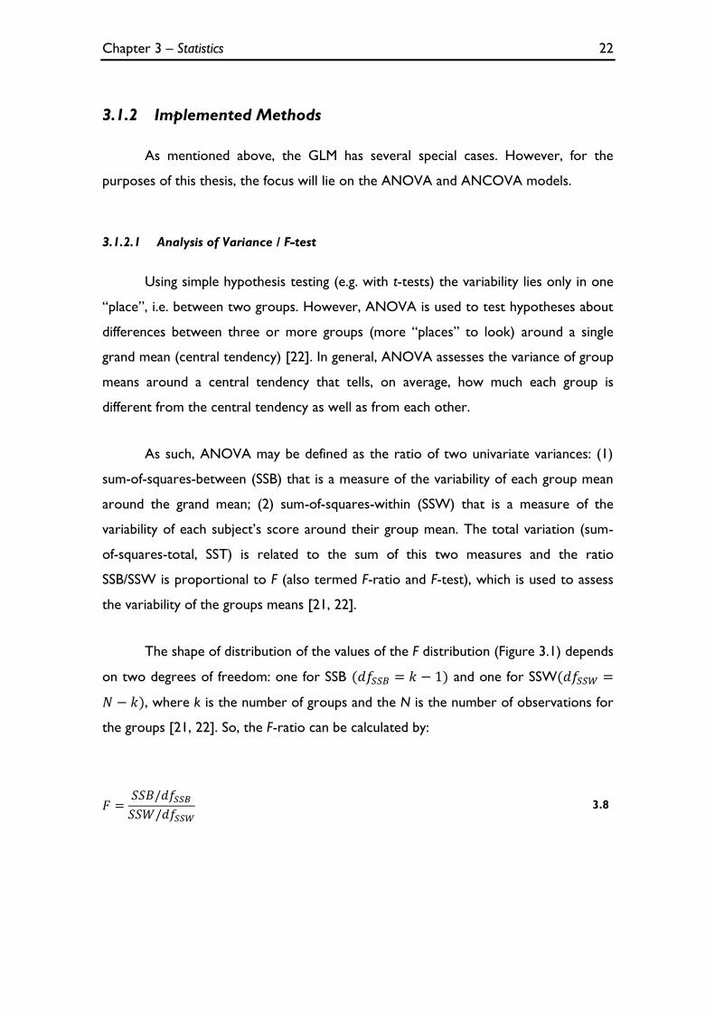
3.1.2.1 Analysis of Variance / F-test
Using simple hypothesis testing (e.g. with t-tests) the variability lies only in one
“place”, i.e. between two groups. However, ANOVA is used to test hypotheses about
differences between three or more groups (more “places” to look) around a single
grand mean (central tendency) [22]. In general, ANOVA assesses the variance of group
means around a central tendency that tells, on average, how much each group is
different from the central tendency as well as from each other.
As such, ANOVA may be defined as the ratio of two univariate variances: (1)
sum-of-squares-between (SSB) that is a measure of the variability of each group mean
around the grand mean; (2) sum-of-squares-within (SSW) that is a measure of the
variability of each subject’s score around their group mean. The total variation (sum-
of-squares-total, SST) is related to the sum of this two measures and the ratio
SSB/SSW is proportional to F (also termed F-ratio and F-test), which is used to assess
the variability of the groups means [21, 22].
The shape of distribution of the values of the F distribution (Figure 3.1) depends
on two degrees of freedom: one for SSB and one for SSW
, where k is the number of groups and the N is the number of observations for
the groups [21, 22]. So, the F-ratio can be calculated by:
3.8

Chapter 3 – Statistics 23
Figure 3.1 - F distribution [23].
Finally, the p-values can be calculated by comparing the F-value with an F
distribution with degrees of freedom. With these p-values, it is possible create a
map of statistical significance and analyze the effects of interest.
Furthermore, within the GLM, the F-ratio can be calculated through the square
of the multiple correlation coefficient R, an important measure of the “goodness of fit”
of a GLM, which provides a measure of the proportion of the variance of the data:
3.9
3.10
As mentioned before, the F value can be converted in an error probability,
where an high F value leads to a low p-value and vice versa (Figure 3.1) [24].

Chapter 3 – Statistics 24
3.1.2.2 Analysis of Covariance
In its most general definition, an ANCOVA may be seen as a combination of a
regression analysis with an ANOVA, i.e. ANCOVA assesses group differences on a DV
after the effects of one or more covariates (“control variables” that are related to the
DV) are statistically accounted for [21, 22, 25]. The prime advantage of using the
ANCOVA model is to minimize the variability of the residual errors that are
associated with covariates, resulting in more precise estimates and more powerful
analysis [21, 25]. Design studies for ANCOVA can be performed by using the
equations 3.2-3.7, while pertinently adjusting the design matrix and contrasts.
Chapter 3 – Statistics 25
3.2 Multivariate Statistics
Multivariate statistical methods are an extension of univariate statistics
methods: instead of performing a series of univariate analysis each with only one DV,
multivariate models allow a single analysis with multiple DVs [21]. This is important
because it allows looking at an analysis in different “views”, providing multiple levels of
inference. Consequently, multivariate methods provide a richer realistic design which
may offer the explanation of more complex research problems [21, 22, 26, 27].
As in univariate statistics, there is a multivariate statistical model that can
integrate various multivariate methods that may be essential in inferential procedures,
i.e. the multivariate general linear model (MGLM).
3.2.1 Multivariate GLM
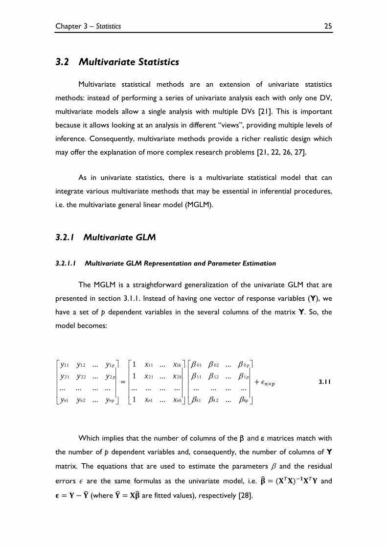
3.2.1.1 Multivariate GLM Representation and Parameter Estimation
The MGLM is a straightforward generalization of the univariate GLM that are
presented in section 3.1.1. Instead of having one vector of response variables (Y), we
have a set of p dependent variables in the several columns of the matrix Y. So, the
model becomes:
npnn
p
p
yyy
yyy
yyy
...
............
...
...
21
22221
11211
=
nkn
k
k
xx
xx
xx
...1
............
...1
...1
1
221
111
kpkk
p
p
...
............
...
...
21
11211
00201
+ 3.11
Which implies that the number of columns of the and matrices match with
the number of p dependent variables and, consequently, the number of columns of Y
matrix. The equations that are used to estimate the parameters and the residual
errors are the same formulas as the univariate model, i.e. and
(where are fitted values), respectively [28].
Chapter 3 – Statistics 26
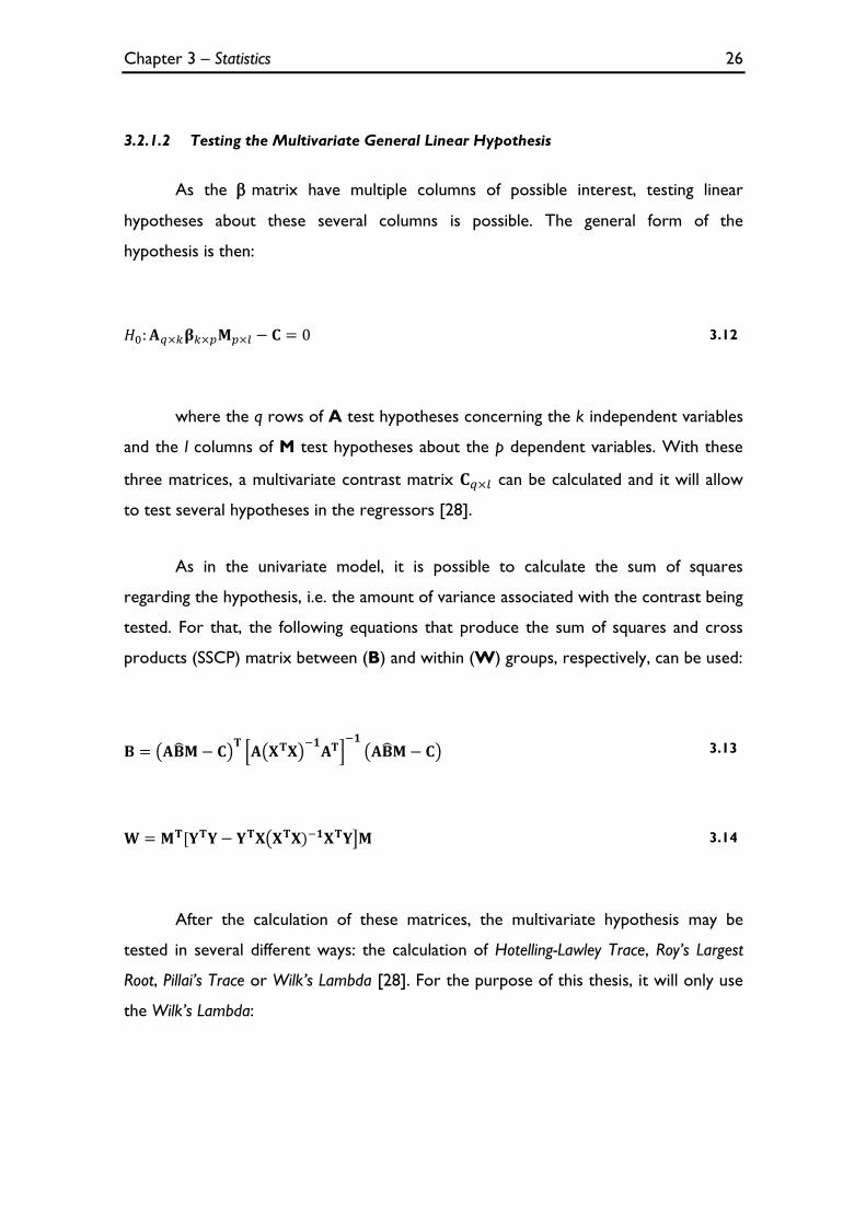
3.2.1.2 Testing the Multivariate General Linear Hypothesis
As the matrix have multiple columns of possible interest, testing linear
hypotheses about these several columns is possible. The general form of the
hypothesis is then:
3.12
where the q rows of A test hypotheses concerning the k independent variables
and the l columns of M test hypotheses about the p dependent variables. With these
three matrices, a multivariate contrast matrix can be calculated and it will allow
to test several hypotheses in the regressors [28].
As in the univariate model, it is possible to calculate the sum of squares
regarding the hypothesis, i.e. the amount of variance associated with the contrast being
tested. For that, the following equations that produce the sum of squares and cross
products (SSCP) matrix between (B) and within (W) groups, respectively, can be used:
3.13
3.14
After the calculation of these matrices, the multivariate hypothesis may be
tested in several different ways: the calculation of Hotelling-Lawley Trace, Roy’s Largest
Root, Pillai’s Trace or Wilk’s Lambda [28]. For the purpose of this thesis, it will only use
the Wilk’s Lambda:

Chapter 3 – Statistics 27
3.15
With this parameter, the approximation based on Wilk’s determinant criterion
to calculate the F ratio can be calculated [28]:
3.16
where q is the number of rows of A and l is the number of columns of M. The
other values are equal to:
where n is the sample size and k is the number of columns of the design matrix.
The degrees of freedom for F are in the numerator and in the
denominator. Finally, as mentioned several times before, the F value can be converted
in an error probability value p and a map of significance can be achieved.
Chapter 3 – Statistics 28
3.2.2 Implemented Methods
3.2.2.1 Hotelling’s T2
The two-sample Hotelling’s T2 is the multivariate extension of the common
two-sample Student’s t-test. Hotelling’s T2 is a special case of multivariate analysis of
variance (MANOVA), just as two-sample t-test is a special case of ANOVA, i.e.
Hotelling’s T2 is used in presence of two dependent variables and one categorical IV
with two levels. Instead of using separate t tests, for each dependent variable, to look
for differences between groups (not legitimate because it inflates type I error due to
unnecessary multiple significance tests), Hotelling’s T2 can be used to if groups differ on
both DVs [21, 22]. As confirmed in the expression below, this involves the
computation of differences in the sample mean vectors ( and and the
multiplication of the pooled variance-covariance matrix ( ) with the sum of the
inverses of the sample size ( and ) [29]:
3.17
3.2.2.2 Multivariate Analysis of Variance
MANOVA is used to test hypotheses about differences between one or more
IVs, among two or more DVs. Therefore, MANOVA can be seen as a multivariate
extension of ANOVA. In general, MANOVA is preferable to performing a series of
ANOVAs, i.e. one for each DV, because multiple ANOVAs can increase the type I
error and the intercorrelations between DVs are ignored in ANOVA. However the
choice of DVs must be well made because these may be redundant, adding complexity
and ambiguity to the analysis [21, 22].
MANOVA designs evaluate whether groups differ on at least one optimally
weighted linear combination of at least two DVs. This can be achieved by using
Chapter 3 – Statistics 29
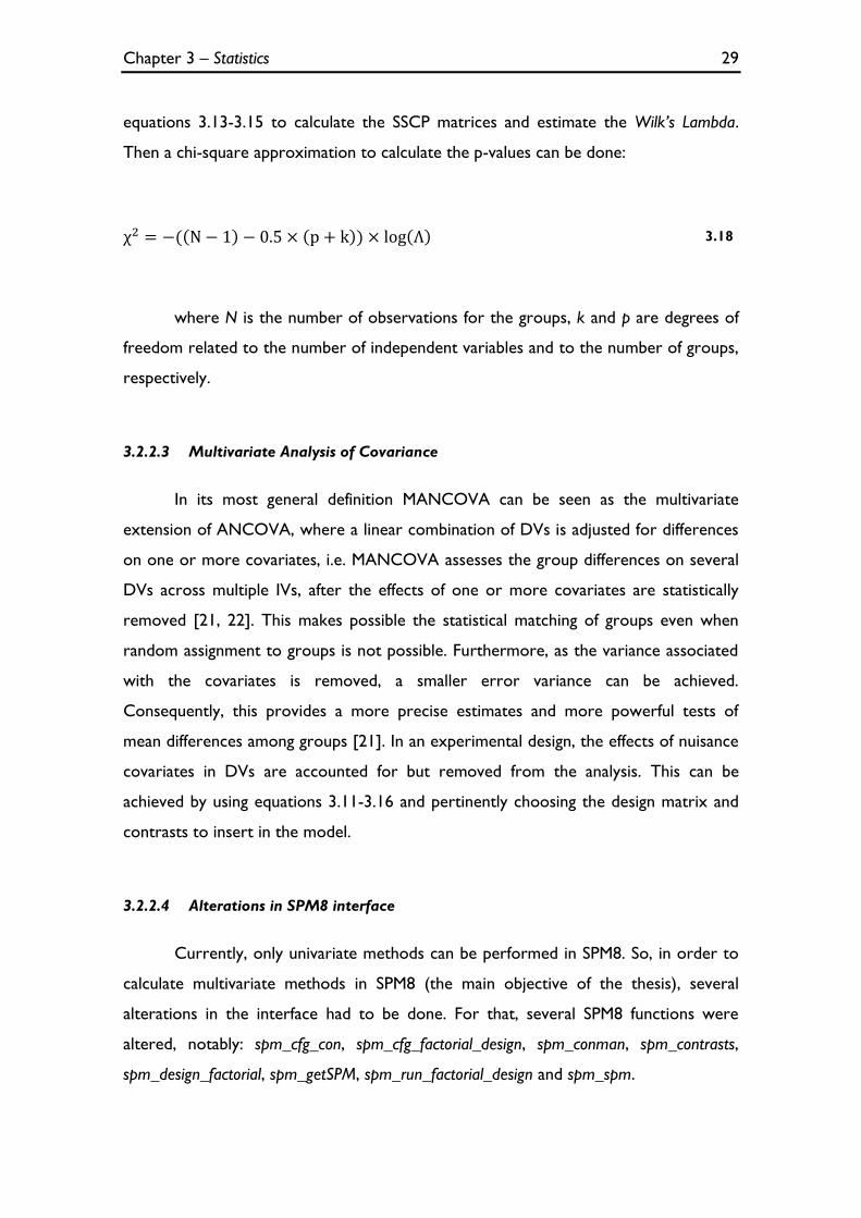
equations 3.13-3.15 to calculate the SSCP matrices and estimate the Wilk’s Lambda.
Then a chi-square approximation to calculate the p-values can be done:
3.18
where N is the number of observations for the groups, k and p are degrees of
freedom related to the number of independent variables and to the number of groups,
respectively.
3.2.2.3 Multivariate Analysis of Covariance
In its most general definition MANCOVA can be seen as the multivariate
extension of ANCOVA, where a linear combination of DVs is adjusted for differences
on one or more covariates, i.e. MANCOVA assesses the group differences on several
DVs across multiple IVs, after the effects of one or more covariates are statistically
removed [21, 22]. This makes possible the statistical matching of groups even when
random assignment to groups is not possible. Furthermore, as the variance associated
with the covariates is removed, a smaller error variance can be achieved.
Consequently, this provides a more precise estimates and more powerful tests of
mean differences among groups [21]. In an experimental design, the effects of nuisance
covariates in DVs are accounted for but removed from the analysis. This can be
achieved by using equations 3.11-3.16 and pertinently choosing the design matrix and
contrasts to insert in the model.
3.2.2.4 Alterations in SPM8 interface
Currently, only univariate methods can be performed in SPM8. So, in order to
calculate multivariate methods in SPM8 (the main objective of the thesis), several
alterations in the interface had to be done. For that, several SPM8 functions were
altered, notably: spm_cfg_con, spm_cfg_factorial_design, spm_conman, spm_contrasts,
spm_design_factorial, spm_getSPM, spm_run_factorial_design and spm_spm.
Chapter 3 – Statistics 30
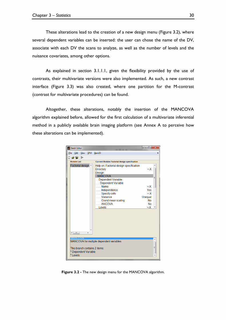
These alterations lead to the creation of a new design menu (Figure 3.2), where
several dependent variables can be inserted: the user can chose the name of the DV,
associate with each DV the scans to analyze, as well as the number of levels and the
nuisance covariates, among other options.
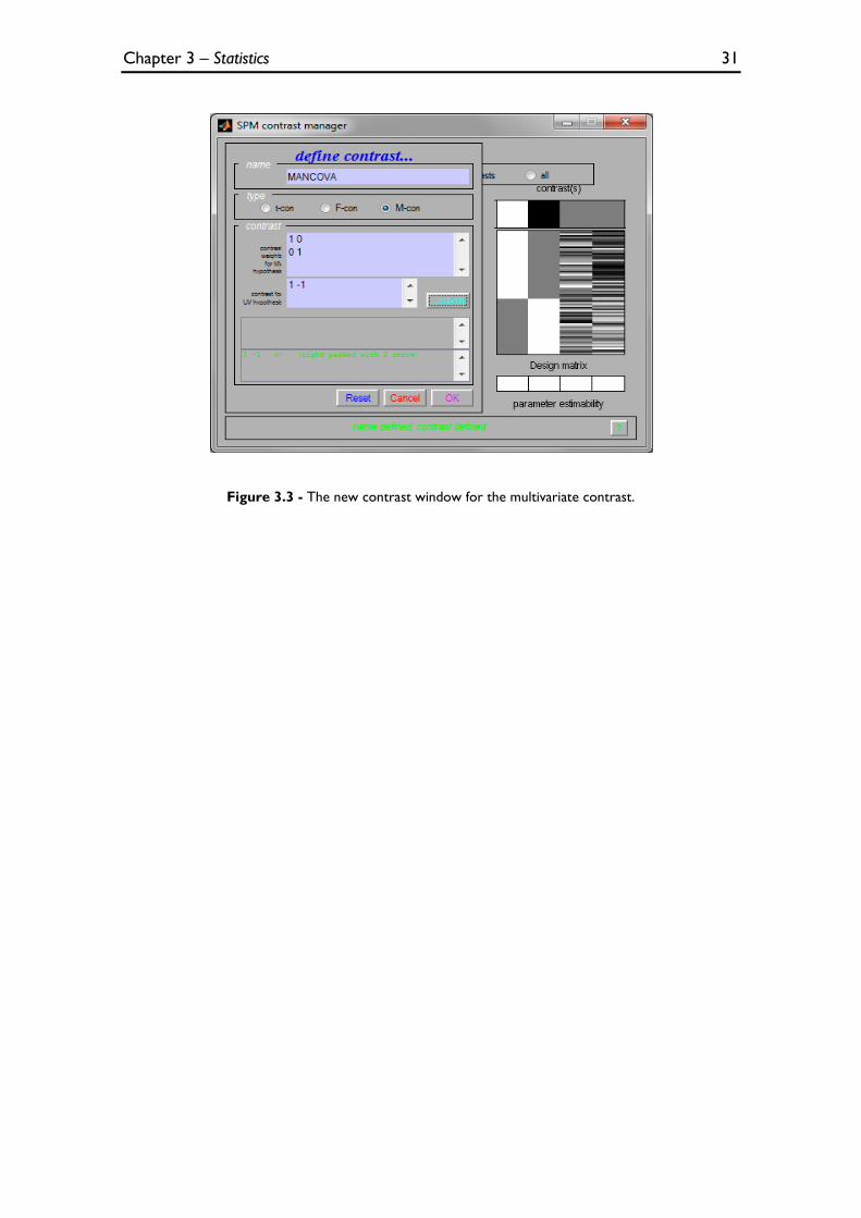
As explained in section 3.1.1.1, given the flexibility provided by the use of
contrasts, their multivariate versions were also implemented. As such, a new contrast
interface (Figure 3.3) was also created, where one partition for the M-contrast
(contrast for multivariate procedures) can be found.
Altogether, these alterations, notably the insertion of the MANCOVA
algorithm explained before, allowed for the first calculation of a multivariate inferential
method in a publicly available brain imaging platform (see Annex A to perceive how
these alterations can be implemented).
Figure 3.2 - The new design menu for the MANCOVA algorithm.
Chapter 3 – Statistics 31
Figure 3.3 - The new contrast window for the multivariate contrast.
Chapter 3 – Statistics 32
3.3 Support Vector Machine
Machine learning can be seen as an alternative to inferential multivariate
analyses and plays an important role on computed techniques for automatic
classification of imaging scans [30]. These algorithms are trained with previously
labelled data (training data). The learned classifier corresponds to a model of the
relationship between the features (i.e. relevant information in the data) and the class
label in the training set [31]. When the size of the training data set is small or when the
number of parameters in the model is large, a cross validation procedure is needed in
order to prevent overfitting. The goal of cross validation is to define a dataset to test
the model in the training phase (i.e. the validation dataset), giving an insight on how the
model will generalize to an independent data set. One example of this is the Leave
One Out (LOO) method, in which the learning algorithm is trained multiple times,
using all but one of the training set data points.
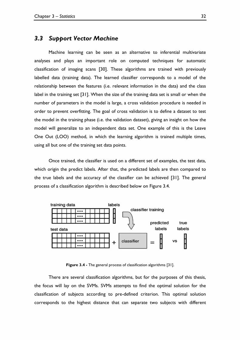
Once trained, the classifier is used on a different set of examples, the test data,
which origin the predict labels. After that, the predicted labels are then compared to
the true labels and the accuracy of the classifier can be achieved [31]. The general
process of a classification algorithm is described below on Figure 3.4.
Figure 3.4 - The general process of classification algorithms [31].
There are several classification algorithms, but for the purposes of this thesis,
the focus will lay on the SVMs. SVMs attempts to find the optimal solution for the
classification of subjects according to pre-defined criterion. This optimal solution
corresponds to the highest distance that can separate two subjects with different
Chapter 3 – Statistics 33
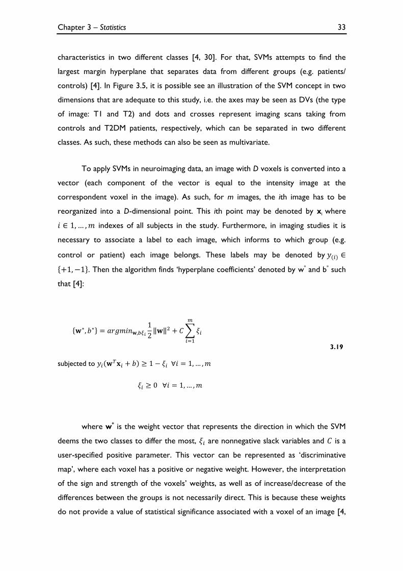
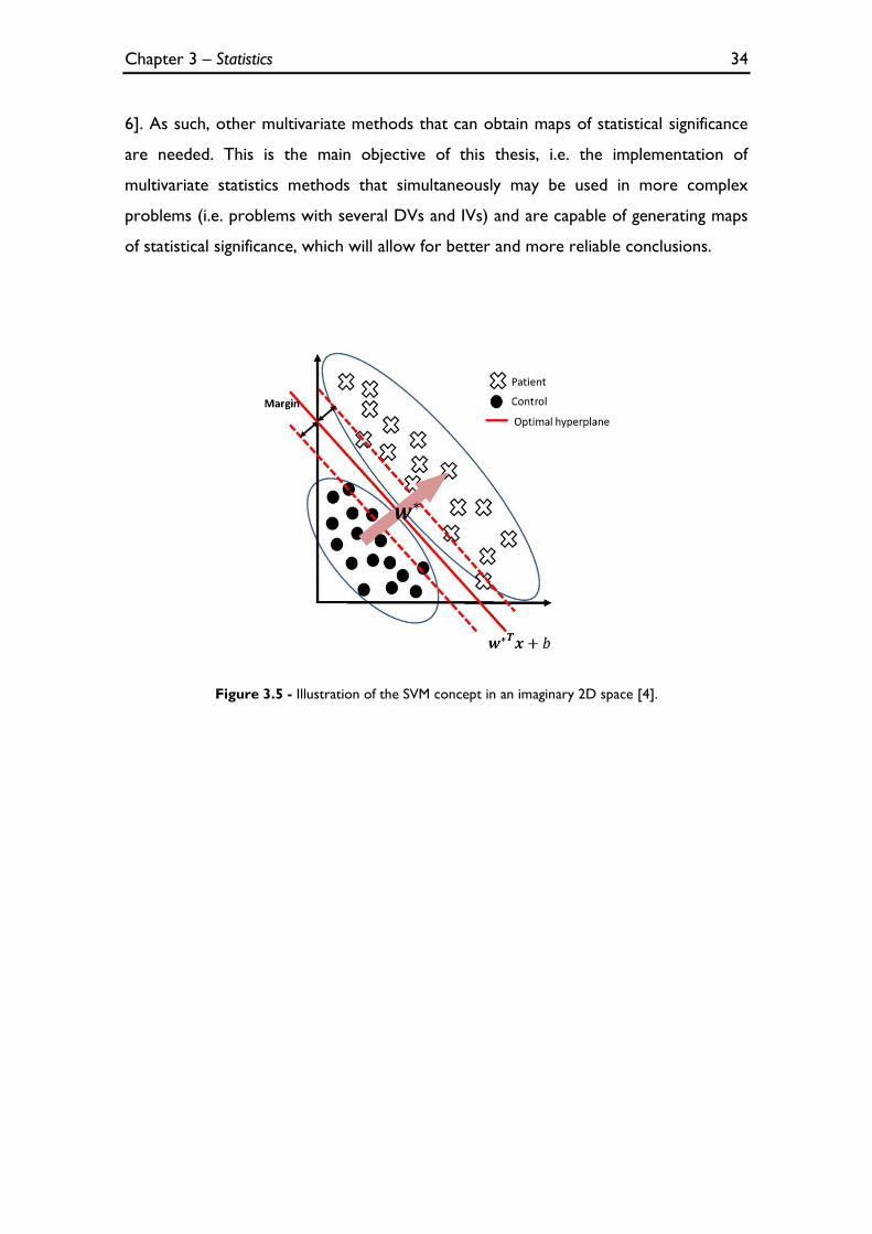
characteristics in two different classes [4, 30]. For that, SVMs attempts to find the
largest margin hyperplane that separates data from different groups (e.g. patients/
controls) [4]. In Figure 3.5, it is possible see an illustration of the SVM concept in two
dimensions that are adequate to this study, i.e. the axes may be seen as DVs (the type
of image: T1 and T2) and dots and crosses represent imaging scans taking from
controls and T2DM patients, respectively, which can be separated in two different
classes. As such, these methods can also be seen as multivariate.
To apply SVMs in neuroimaging data, an image with D voxels is converted into a
vector (each component of the vector is equal to the intensity image at the
correspondent voxel in the image). As such, for m images, the ith image has to be
reorganized into a D-dimensional point. This ith point may be denoted by xi where
indexes of all subjects in the study. Furthermore, in imaging studies it is
necessary to associate a label to each image, which informs to which group (e.g.
control or patient) each image belongs. These labels may be denoted by
. Then the algorithm finds ‘hyperplane coefficients’ denoted by w* and b* such
that [4]:
subjected to
3.19
where w* is the weight vector that represents the direction in which the SVM
deems the two classes to differ the most, are nonnegative slack variables and is a
user-specified positive parameter. This vector can be represented as ‘discriminative
map’, where each voxel has a positive or negative weight. However, the interpretation
of the sign and strength of the voxels’ weights, as well as of increase/decrease of the
differences between the groups is not necessarily direct. This is because these weights
do not provide a value of statistical significance associated with a voxel of an image [4,
Chapter 3 – Statistics 34
6]. As such, other multivariate methods that can obtain maps of statistical significance
are needed. This is the main objective of this thesis, i.e. the implementation of
multivariate statistics methods that simultaneously may be used in more complex
problems (i.e. problems with several DVs and IVs) and are capable of generating maps
of statistical significance, which will allow for better and more reliable conclusions.
Figure 3.5 - Illustration of the SVM concept in an imaginary 2D space [4].
Chapter 4 – Implementation 35
Chapter 4
Implementation
4.1 Methods
4.1.1 Patient Selection
Thirty-four participants with T2DM and forty-two gender matched control
subjects were recruited. Controls were recruited from the general population of
Hospital or University staff, and T2DM patients from the Endocrinology Department,
of the University Hospital (Centro Hospitalar e Universitário de Coimbra). T2DM
patients presented with the condition for at least one year prior to the
commencement of this study, and were diagnosed using standard WHO (World
Health Organization) criteria [32] [33]. Participants were included between November
2011 and November 2013. Exclusion criteria for both groups were severe
cardiovascular disease (trasient ischemic attack or stroke), neurologic diseases
unrelated to diabetes likely to affect cognitive functions, known history of psychiatric
disease and alchool abuse.
4.1.2 Image Acquisition
The MR scans were acquired at the Portuguese Brain Imaging Network facilities
in Coimbra, Portugal, on a 3T research scanner (Magnetom TIM Trio, Siemens) using a
phased array 12-channel birdcage head coil (Siemens).
For each participant, a 3D anatomical MPRAGE (magnetization-prepared rapid
gradient echo) scan was acquired using a standard T1-weighted gradient echo pulse
Chapter 4 – Implementation 36
sequence with TR = 2530 ms, TE = 3.42 ms, TI = 1100 ms, flip angle 7°, 176 single shot
slices with voxel size 1x1x1 mm, and FOV (field of view) 256 mm. True 3D, high-
resolution, T2-weighted images will be acquired. The turbo spin echo with variable flip-
angle distribution (sampling perfection with application optimized contrasts using
different flip angle evolution; SPACE) pulse sequence was used with the following scan
parameters: TR/TE/NEX = 3200ms/450ms/2; matrix, 192x192x144 slices; voxel
resolution 1.25x1.25x1.25mm3.
4.1.3 SPM Analyses
Images were processed with SPM8, running on Matlab R2012a® (The Math-
Works, Inc., Natick, MA), in order to perform the VBM analysis. This included spatial
normalization and GM segmentation using the unified segmentation algorithm,
explained before. Modulated GM segments, registered to the ICBM152 template, were
then smoothed with an 8mm full width at half maximum (FWHM) three-dimensional
Gaussian kernel to ensure the normality of the data.
The statistical analyses performed in SPM8 can be divided in two types:
univariate and multivariate. For univariate analyses (ANOVA and ANCOVA, seen in
the section 4.2.1), the GLM was adapted to the study in terms of design and contrasts.
With the alterations mentioned in 3.2.2.4, a multivariate analysis (MANCOVA) was
performed.
4.1.4 Image analyses outside SPM
The results of all implemented methods presented in chapter 3 were obtained
with functions scripted in Matlab, outside the framework of SPM. As above, two type
of analysis were performed: the univariate and multivariate analyses.
4.1.5 Overlap of results with a high resolution image
As the results obtained in Matlab, outside the framework of SPM, do not
provide good spatial localization of the differences detected, it was necessary to create
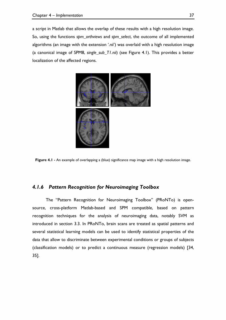
Chapter 4 – Implementation 37
a script in Matlab that allows the overlap of these results with a high resolution image.
So, using the functions spm_orthviews and spm_select, the outcome of all implemented
algorithms (an image with the extension ‘.nii’) was overlaid with a high resolution image
(a canonical image of SPM8, single_sub_T1.nii) (see Figure 4.1). This provides a better
localization of the affected regions.
Figure 4.1 - An example of overlapping a (blue) significance map image with a high resolution image.
4.1.6 Pattern Recognition for Neuroimaging Toolbox
The “Pattern Recognition for Neuroimaging Toolbox” (PRoNTo) is open-
source, cross-platform Matlab-based and SPM compatible, based on pattern
recognition techniques for the analysis of neuroimaging data, notably SVM as
introduced in section 3.3. In PRoNTo, brain scans are treated as spatial patterns and
several statistical learning models can be used to identify statistical properties of the
data that allow to discriminate between experimental conditions or groups of subjects
(classification models) or to predict a continuous measure (regression models) [34,
35].
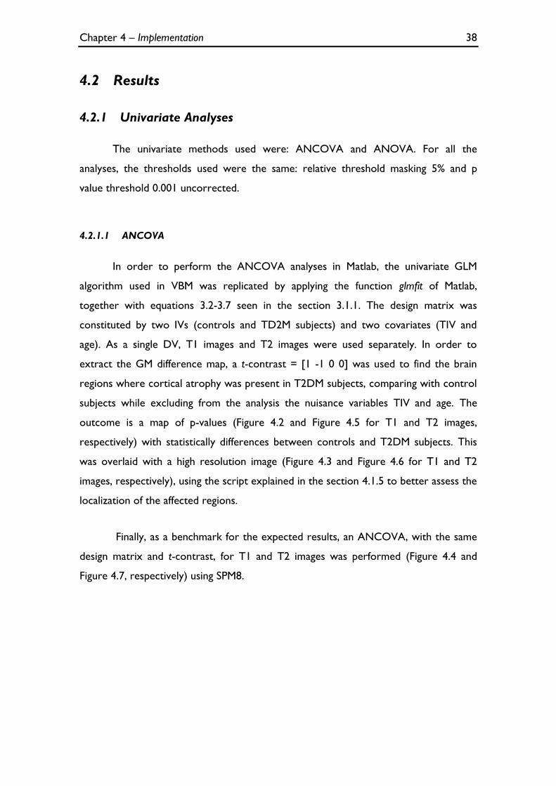
Chapter 4 – Implementation 38
4.2 Results
4.2.1 Univariate Analyses
The univariate methods used were: ANCOVA and ANOVA. For all the
analyses, the thresholds used were the same: relative threshold masking 5% and p
value threshold 0.001 uncorrected.
4.2.1.1 ANCOVA
In order to perform the ANCOVA analyses in Matlab, the univariate GLM
algorithm used in VBM was replicated by applying the function glmfit of Matlab,
together with equations 3.2-3.7 seen in the section 3.1.1. The design matrix was
constituted by two IVs (controls and TD2M subjects) and two covariates (TIV and
age). As a single DV, T1 images and T2 images were used separately. In order to
extract the GM difference map, a t-contrast = [1 -1 0 0] was used to find the brain
regions where cortical atrophy was present in T2DM subjects, comparing with control
subjects while excluding from the analysis the nuisance variables TIV and age. The
outcome is a map of p-values (Figure 4.2 and Figure 4.5 for T1 and T2 images,
respectively) with statistically differences between controls and T2DM subjects. This
was overlaid with a high resolution image (Figure 4.3 and Figure 4.6 for T1 and T2
images, respectively), using the script explained in the section 4.1.5 to better assess the
localization of the affected regions.
Finally, as a benchmark for the expected results, an ANCOVA, with the same
design matrix and t-contrast, for T1 and T2 images was performed (Figure 4.4 and
Figure 4.7, respectively) using SPM8.
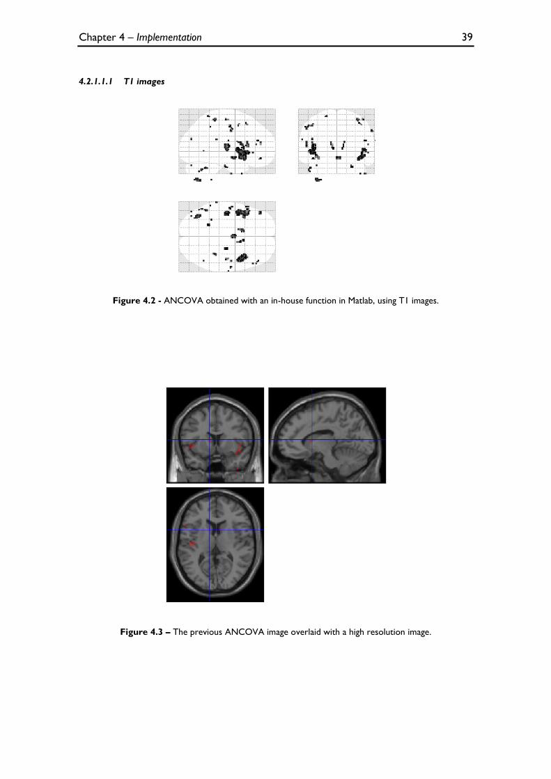
Chapter 4 – Implementation 39
4.2.1.1.1 T1 images
Figure 4.2 - ANCOVA obtained with an in-house function in Matlab, using T1 images.
Figure 4.3 – The previous ANCOVA image overlaid with a high resolution image.
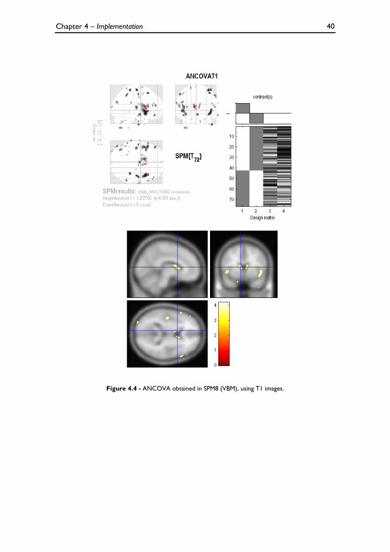
Chapter 4 – Implementation 40
Figure 4.4 - ANCOVA obtained in SPM8 (VBM), using T1 images.
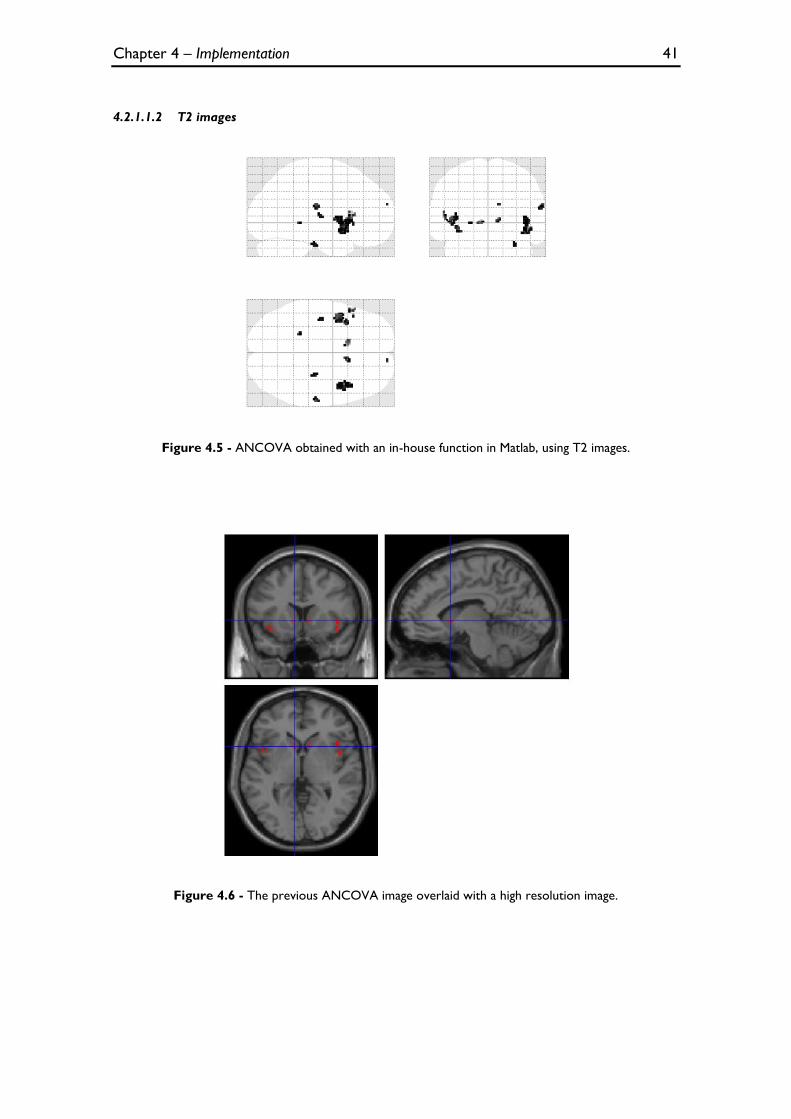
Chapter 4 – Implementation 41
4.2.1.1.2 T2 images
Figure 4.5 - ANCOVA obtained with an in-house function in Matlab, using T2 images.
Figure 4.6 - The previous ANCOVA image overlaid with a high resolution image.
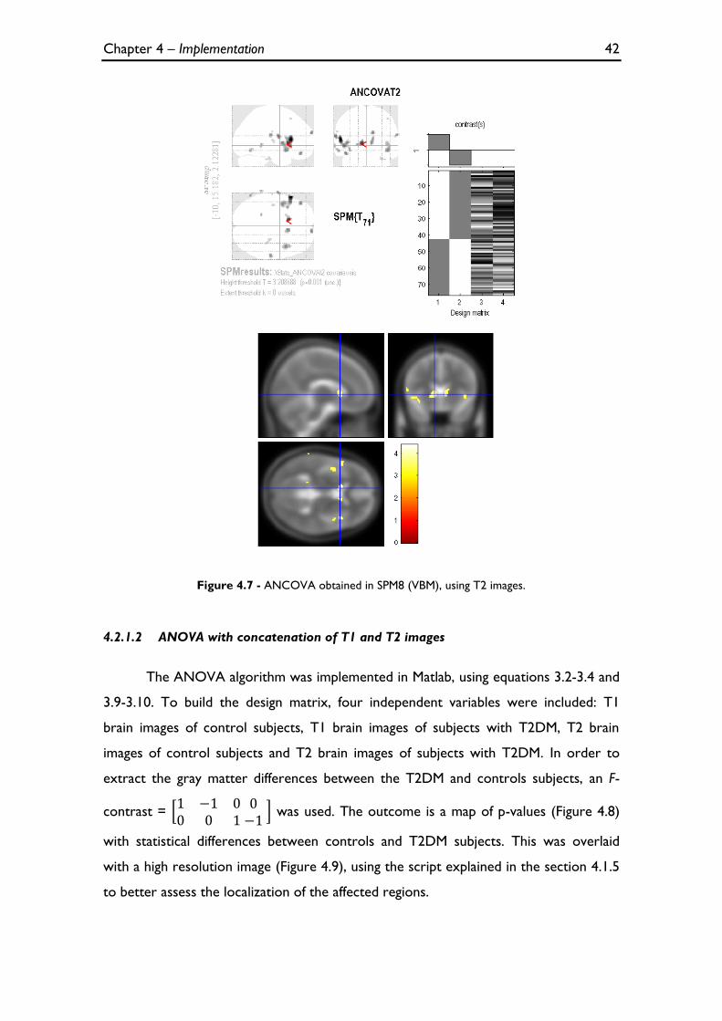
Chapter 4 – Implementation 42
Figure 4.7 - ANCOVA obtained in SPM8 (VBM), using T2 images.
4.2.1.2 ANOVA with concatenation of T1 and T2 images
The ANOVA algorithm was implemented in Matlab, using equations 3.2-3.4 and
3.9-3.10. To build the design matrix, four independent variables were included: T1
brain images of control subjects, T1 brain images of subjects with T2DM, T2 brain
images of control subjects and T2 brain images of subjects with T2DM. In order to
extract the gray matter differences between the T2DM and controls subjects, an F-
contrast =
was used. The outcome is a map of p-values (Figure 4.8)
with statistical differences between controls and T2DM subjects. This was overlaid
with a high resolution image (Figure 4.9), using the script explained in the section 4.1.5
to better assess the localization of the affected regions.
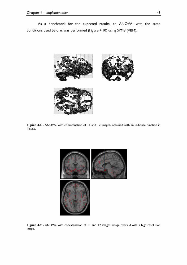
Chapter 4 – Implementation 43
As a benchmark for the expected results, an ANOVA, with the same
conditions used before, was performed (Figure 4.10) using SPM8 (VBM).
Figure 4.8 - ANOVA, with concatenation of T1 and T2 images, obtained with an in-house function in
Matlab.
Figure 4.9 - ANOVA, with concatenation of T1 and T2 images, image overlaid with a high resolution
image.
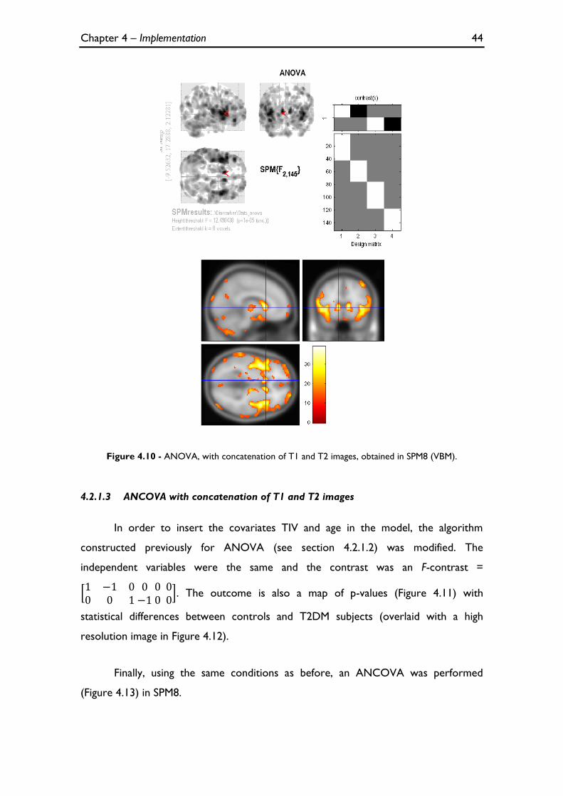
Chapter 4 – Implementation 44
Figure 4.10 - ANOVA, with concatenation of T1 and T2 images, obtained in SPM8 (VBM).
4.2.1.3 ANCOVA with concatenation of T1 and T2 images
In order to insert the covariates TIV and age in the model, the algorithm
constructed previously for ANOVA (see section 4.2.1.2) was modified. The
independent variables were the same and the contrast was an F-contrast =
. The outcome is also a map of p-values (Figure 4.11) with
statistical differences between controls and T2DM subjects (overlaid with a high
resolution image in Figure 4.12).
Finally, using the same conditions as before, an ANCOVA was performed
(Figure 4.13) in SPM8.
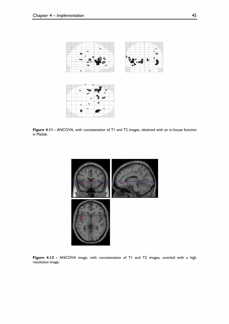
Chapter 4 – Implementation 45
Figure 4.11 - ANCOVA, with concatenation of T1 and T2 images, obtained with an in-house function
in Matlab.
Figure 4.12 - ANCOVA image, with concatenation of T1 and T2 images, overlaid with a high
resolution image.
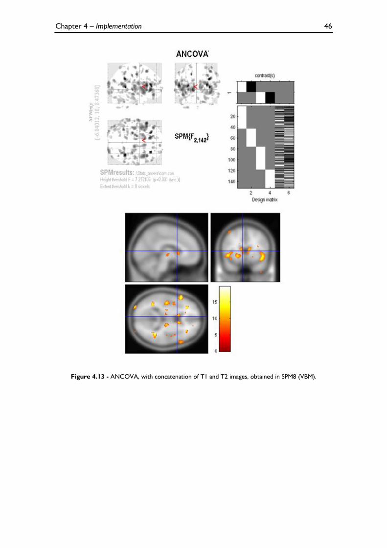
Chapter 4 – Implementation 46
Figure 4.13 - ANCOVA, with concatenation of T1 and T2 images, obtained in SPM8 (VBM).
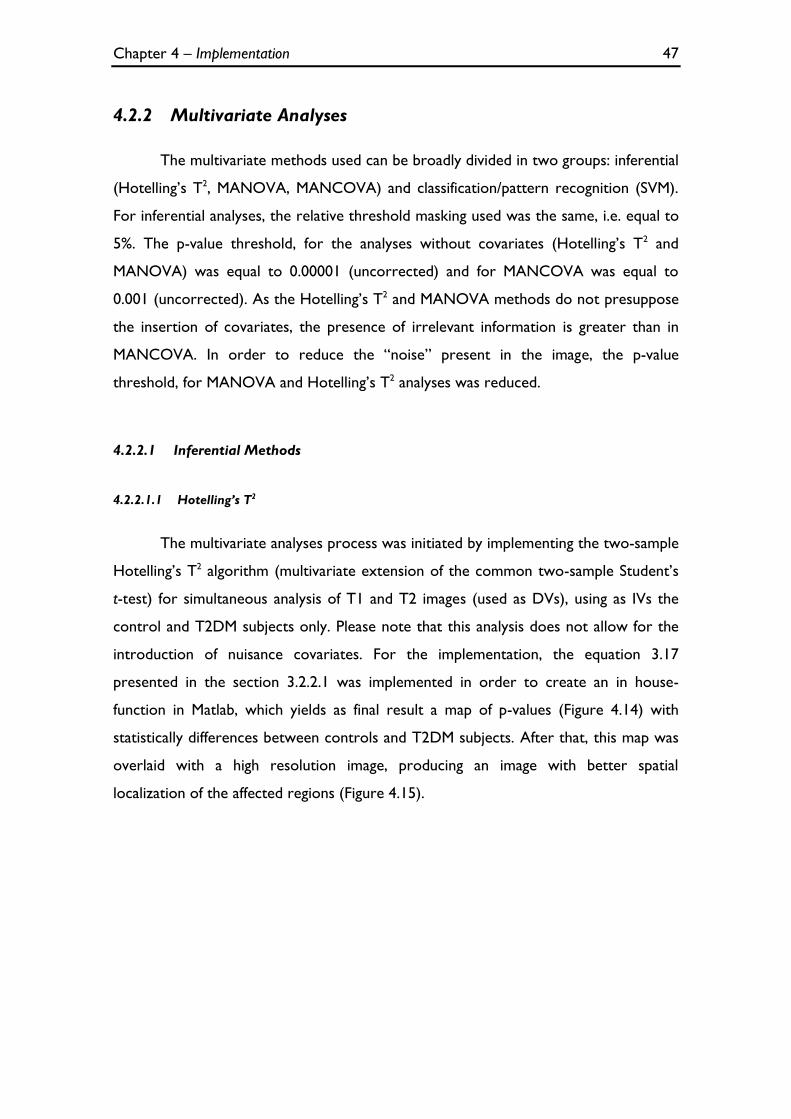
Chapter 4 – Implementation 47
4.2.2 Multivariate Analyses
The multivariate methods used can be broadly divided in two groups: inferential
(Hotelling’s T2, MANOVA, MANCOVA) and classification/pattern recognition (SVM).
For inferential analyses, the relative threshold masking used was the same, i.e. equal to
5%. The p-value threshold, for the analyses without covariates (Hotelling’s T2 and
MANOVA) was equal to 0.00001 (uncorrected) and for MANCOVA was equal to
0.001 (uncorrected). As the Hotelling’s T2 and MANOVA methods do not presuppose
the insertion of covariates, the presence of irrelevant information is greater than in
MANCOVA. In order to reduce the “noise” present in the image, the p-value
threshold, for MANOVA and Hotelling’s T2 analyses was reduced.
4.2.2.1 Inferential Methods
4.2.2.1.1 Hotelling’s T2
The multivariate analyses process was initiated by implementing the two-sample
Hotelling’s T2 algorithm (multivariate extension of the common two-sample Student’s
t-test) for simultaneous analysis of T1 and T2 images (used as DVs), using as IVs the
control and T2DM subjects only. Please note that this analysis does not allow for the
introduction of nuisance covariates. For the implementation, the equation 3.17
presented in the section 3.2.2.1 was implemented in order to create an in house-
function in Matlab, which yields as final result a map of p-values (Figure 4.14) with
statistically differences between controls and T2DM subjects. After that, this map was
overlaid with a high resolution image, producing an image with better spatial
localization of the affected regions (Figure 4.15).
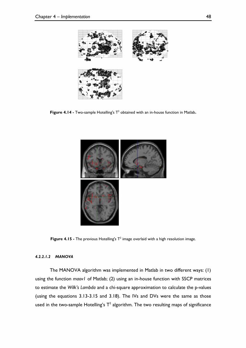
Chapter 4 – Implementation 48
Figure 4.14 - Two-sample Hotelling's T2 obtained with an in-house function in Matlab.
Figure 4.15 - The previous Hotelling's T2 image overlaid with a high resolution image.
4.2.2.1.2 MANOVA
The MANOVA algorithm was implemented in Matlab in two different ways: (1)
using the function maov1 of Matlab; (2) using an in-house function with SSCP matrices
to estimate the Wilk’s Lambda and a chi-square approximation to calculate the p-values
(using the equations 3.13-3.15 and 3.18). The IVs and DVs were the same as those
used in the two-sample Hotelling’s T2 algorithm. The two resulting maps of significance
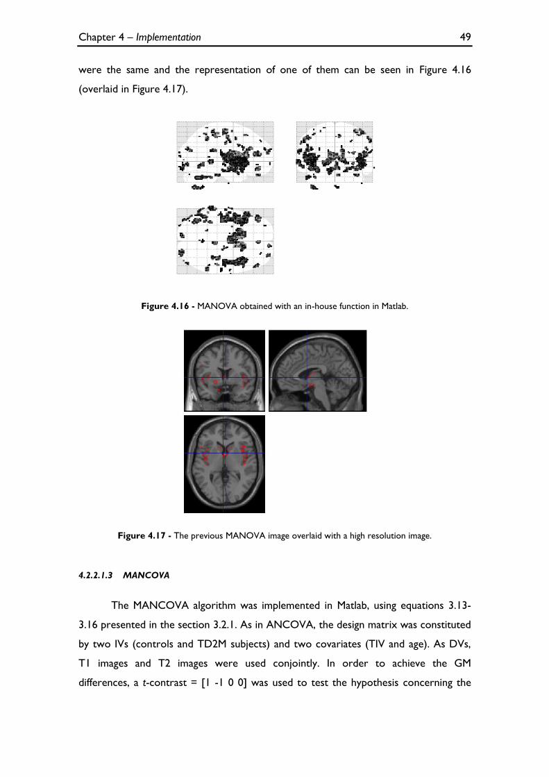
Chapter 4 – Implementation 49
were the same and the representation of one of them can be seen in Figure 4.16
(overlaid in Figure 4.17).
Figure 4.16 - MANOVA obtained with an in-house function in Matlab.
Figure 4.17 - The previous MANOVA image overlaid with a high resolution image.
4.2.2.1.3 MANCOVA
The MANCOVA algorithm was implemented in Matlab, using equations 3.13-
3.16 presented in the section 3.2.1. As in ANCOVA, the design matrix was constituted
by two IVs (controls and TD2M subjects) and two covariates (TIV and age). As DVs,
T1 images and T2 images were used conjointly. In order to achieve the GM
differences, a t-contrast = [1 -1 0 0] was used to test the hypothesis concerning the
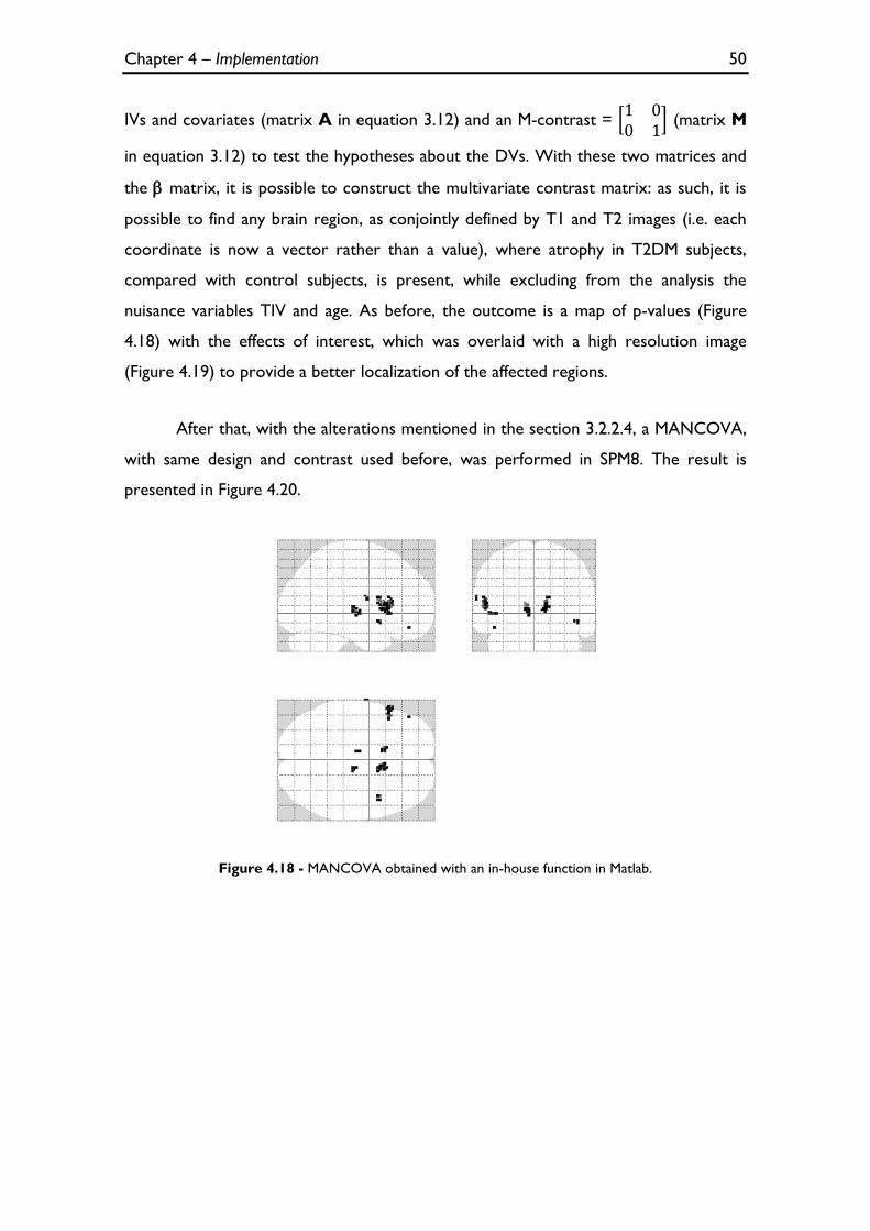
Chapter 4 – Implementation 50
IVs and covariates (matrix A in equation 3.12) and an M-contrast =
(matrix M
in equation 3.12) to test the hypotheses about the DVs. With these two matrices and
the matrix, it is possible to construct the multivariate contrast matrix: as such, it is
possible to find any brain region, as conjointly defined by T1 and T2 images (i.e. each
coordinate is now a vector rather than a value), where atrophy in T2DM subjects,
compared with control subjects, is present, while excluding from the analysis the
nuisance variables TIV and age. As before, the outcome is a map of p-values (Figure
4.18) with the effects of interest, which was overlaid with a high resolution image
(Figure 4.19) to provide a better localization of the affected regions.
After that, with the alterations mentioned in the section 3.2.2.4, a MANCOVA,
with same design and contrast used before, was performed in SPM8. The result is
presented in Figure 4.20.
Figure 4.18 - MANCOVA obtained with an in-house function in Matlab.
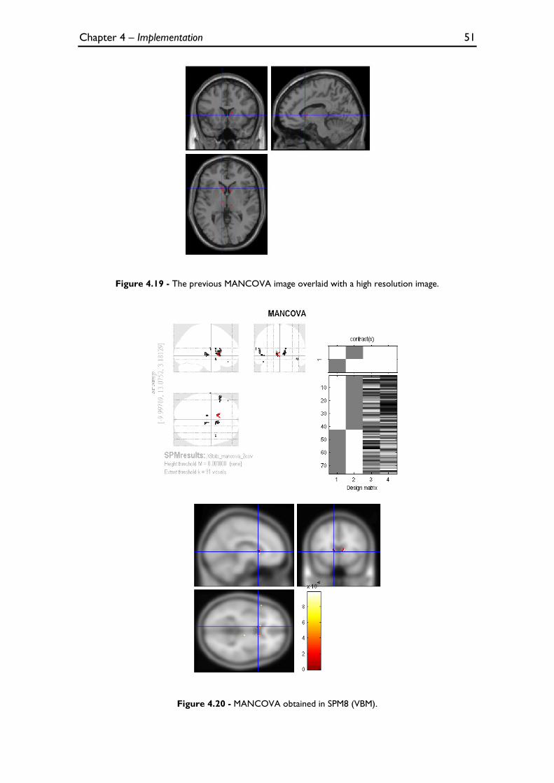
Chapter 4 – Implementation 51
Figure 4.19 - The previous MANCOVA image overlaid with a high resolution image.
Figure 4.20 - MANCOVA obtained in SPM8 (VBM).
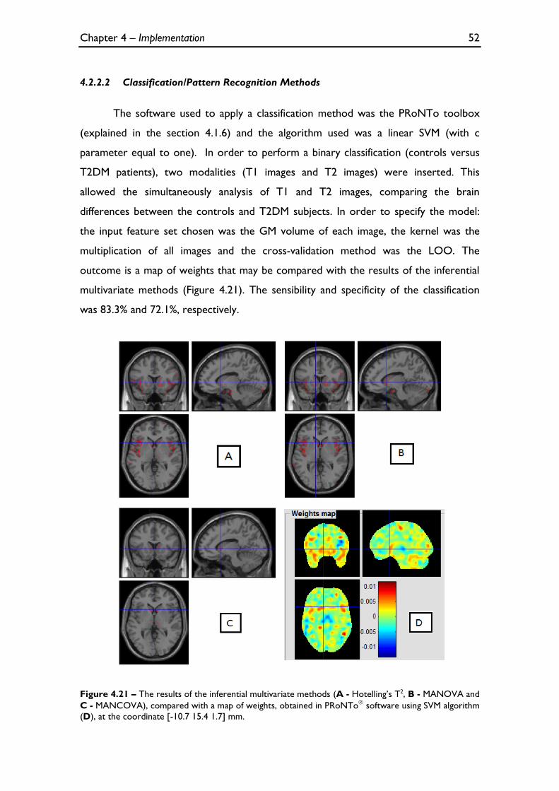
Chapter 4 – Implementation 52
4.2.2.2 Classification/Pattern Recognition Methods
The software used to apply a classification method was the PRoNTo toolbox
(explained in the section 4.1.6) and the algorithm used was a linear SVM (with c
parameter equal to one). In order to perform a binary classification (controls versus
T2DM patients), two modalities (T1 images and T2 images) were inserted. This
allowed the simultaneously analysis of T1 and T2 images, comparing the brain
differences between the controls and T2DM subjects. In order to specify the model:
the input feature set chosen was the GM volume of each image, the kernel was the
multiplication of all images and the cross-validation method was the LOO. The
outcome is a map of weights that may be compared with the results of the inferential
multivariate methods (Figure 4.21). The sensibility and specificity of the classification
was 83.3% and 72.1%, respectively.
Figure 4.21 – The results of the inferential multivariate methods (A - Hotelling’s T2, B - MANOVA and
C - MANCOVA), compared with a map of weights, obtained in PRoNTo software using SVM algorithm
(D), at the coordinate [-10.7 15.4 1.7] mm.
Chapter 5 – Discussion & Conclusions 53
Chapter 5
Discussion & Conclusions
As stated in the introduction, this thesis had three main goals, which were
pursued in phases:
1) Replicate the univariate VBM analyses between controls and T2DM patients
in Matlab, using SPM8 software as a reference;
2) Explore and implement multivariate methods that can integrate information
from T1 and T2 images, contrasting controls to T2DM patients;
3) Insertion of these multivariate algorithms into the pipeline of SPM8 so that
it can be used in further multimodal studies.
All these goals were successfully accomplished, as further expanded below.
5.1 Univariate Analyses and Type 2 Diabetes Mellitus
In the first phase, the standard GLM algorithm used in SPM8 was coded, making
it possible to perform an ANCOVA, using only T1 or T2 images, and ANOVA and
ANCOVA with concatenation of T1 and T2 images. In both univariate analyses, the
results obtained with the replicated algorithm were identical to the results obtained
with the standard SPM8 version used for VBM (see sections 4.2.1.1, 4.2.1.2 and
4.2.1.3).
In ANCOVA for separate analysis of T1 and T2 images, the structural and
vascular changes are clearly visible in T1 and T2 images, respectively, and they are
more noticeable in the limbic lobe, sub-lobar, insular and temporal areas (brain areas
Chapter 5 – Discussion & Conclusions 54
responsible for emotional and cognitive functions), bilaterally. These results are in
agreement with the expected brain alterations in T2DM patients, described in the
literature [7-11]. Furthermore, other publications corroborate these results: in a study
where a relatively large population (350 patients and 364 controls) was used, a pattern
of GM loss was found mainly in the medial temporal, anterior cingulated and medial
frontal lobes [36]; and in a recent study where similar changes, particularly in the
limbic system and temporo-parietal lobes (cingulum, insular area, hippocampus) are
described [37].
The results of the ANOVA with the concatenation of T1 and T2 images were
not as specific (see section 4.2.1.2) because the exclusion of the nuisance covariates
from the analysis leads to more ‘noise’ in the images. In order to surpass this
limitation, the script was altered and the insertion of the covariates was performed
(see section 4.2.1.3). These results are comparable with the results of the ANCOVA
analyses using T1 and T2 images separately (section 4.2.1.1), i.e. the atrophic tissue is
also predominant in the limbic lobe, sub-lobar, insular and temporal areas.
5.2 Multivariate Analyses and Type 2 Diabetes Mellitus
In the second phase, three inferential multivariate methods were implemented
(Hotelling’s T2, MANOVA and MANCOVA). Although the results of these analyses
seem different, they are identical, but as MANOVA and Hotelling’s methods do not
presuppose the insertion of the nuisance covariates and MANCOVA does, the latter
may lead to ‘cleaner’ results, i.e. more specific results, with less false positives.
Nevertheless, the differences in cortical tissue are also visible in the three
analyses, being more noticeable in the limbic lobe, sub-lobar, insular and temporal
areas as well (see sections 4.2.2.1.1, 4.2.2.1.2 and 4.2.2.1.3). Though the univariate
analyses lead to clinically sensible results, the multivariate analyses may lead to more
powerful results without a loss of specificity: in fact, the atrophic brain areas detected
seem more restricted (e.g. compare the MANOVA versus ANOVA results and
MANCOVA e ANCOVA results). It is worth underlining that multivariate analyses
Chapter 5 – Discussion & Conclusions 55
allow for the assessment of data from different “views”, providing greater
discriminative power, which may lead to enhanced inference.
It cannot be excluded, however, that the correlation between T1 and T2 (both
DVs used herein) may have pose a hindrance to the application of the multivariate
methods: this is a key limitation of this work; indeed, it must be acknowledged that a
number of presuppositions that should have been in place to ensure the validity of the
application of these parametric multivariate tests – apart from the normality of the
data, which was ensure through spatial smoothing – were not tested. This is, however,
not critical in this “proof of concept” (PoC) stage, but will be required in future work.
After that, these multivariate results were compared with a single SVM result
(Figure 4.21). Instead a map of significance, the latter result is a map of weight
coefficients. It is possible to perceive the brain differences between control subjects
and T2DM subjects: in this case, the red regions can be interpreted, though not with
full certainty, as regions where the GM volume is greater in controls than T2DM
patients. Seen from this perspective, this map is somewhat similar to the other maps
obtained with the inferential multivariate methods, especially with Hotelling’s T2 and
MANOVA – this may be so because the nuisance covariates were not introduced in
the SVM data (Figure 4.21).
5.3 Possible Future SPM8 toolbox
In the last phase, in which proved to be the most challenging aspect of this
thesis, the alterations in the SPM8 functions, mentioned in the section 3.2.2.4, were
implemented, notably the creation of the design menu and the contrast window. With
all of these alterations, the MANCOVA algorithm was fully inserted in SPM8 and the
first multivariate result within this software (Figure 4.20) was obtained. This thesis is
the groundwork for a publicly available multivariate statistics toolbox, to be inserted in
this widely used brain imaging platform.
Chapter 5 – Discussion & Conclusions 56
5.4 Limitations & Future work
It is crucial understand that this work is a “proof of concept”, i.e. the main
objective of this thesis is not create a perfect algorithm to prove the brain alterations
in T2DM, but demonstrate that it is possible to implement inferential multivariate
methods in an accessible programming language (Matlab) while inserting these
algorithms in a toolbox for a widely used brain imaging platform such as SPM8. As
mentioned before, given time and data constraints, volumetric T1 and T2 brain scans
obtained from subjects who participated in the Diamarker project were used. The
implementation was adapted to these limited data, not taking into account difficulties
that may arise from using multiple modalities (e.g. PET and fMRI), notably different scan
space and resolution.
Additionally, as mentioned above, some of the pre-requisites to perform
statistical tests were not tested, notably the correlation between DVs. Future work
will focus on surpassing these limitations and preparing the methods to be applied in
multimodal studies.
References 57
References
1. Aine, C.J., A conceptual overview and critique of functional neuroimaging techniques in humans: I. MRI/FMRI and PET. Crit Rev Neurobiol, 1995. 9(2-3): p. 229-309.
2. Luo, W.L. and T.E. Nichols, Diagnosis and exploration of massively univariate neuroimaging models. Neuroimage, 2003. 19(3): p. 1014-32.
3. Friston, K.J., Statistical parametric maps in functional imaging: A General Linear Approach. Human Brain Mapping, 1995. 2: p. 189-210.
4. Gaonkar, B. and C. Davatzikos, Analytic estimation of statistical significance maps for support vector machine based multi-variate image analysis and classification. Neuroimage, 2013. 78: p. 270-83.
5. Liu, F., et al., Inter-modality relationship constrained multi-modality multi-task feature selection for Alzheimer's Disease and mild cognitive impairment identification. Neuroimage, 2014. 84: p. 466-75.
6. Duarte, J.V., et al., Multivariate pattern analysis reveals subtle brain anomalies relevant to the cognitive phenotype in neurofibromatosis type 1. Human Brain Mapping, 2014. 35(1): p. 89-106.
7. Guerrero-Berroa, E., J. Schmeidler, and M.S. Beeri, Neuropathology of type 2 diabetes: a short review on insulin-related mechanisms. Eur Neuropsychopharmacol, 2014.
8. Wrighten, S.A., et al., A look inside the diabetic brain: Contributors to diabetes-induced brain aging. Biochim Biophys Acta, 2009. 1792(5): p. 444-453.
9. van Harten, B., et al., Brain lesions on MRI in elderly patients with type 2 diabetes mellitus. Eur Neurol, 2007. 57(2): p. 70-4.
10. Manschot, S.M., et al., Brain magnetic resonance imaging correlates of impaired cognition in patients with type 2 diabetes. Diabetes, 2006. 55(4): p. 1106-13.
11. den Heijer, T., et al., Type 2 diabetes and atrophy of medial temporal lobe structures on brain MRI. Diabetologia, 2003. 46(12): p. 1604-10.
References 58
12. MacDonald-Jankowski, D.S., Magnetic Resonance Imaging. Part 1: the Basic Principles. Asian Journal of Oral and Maxillofacial Surgery, 2006. 18(3): p. 165-171.
13. Glassman, N.R., Magnetic Resonance Imaging. Journal of Consumer Health On the Internet, 2010. 14(3): p. 308-321.
14. Sands, M.J. and A. Levitin, Basics of magnetic resonance imaging. Seminars in Vascular Surgery, 2004. 17(2): p. 66-82.
15. van Geuns, R.-J.M., et al., Basic Principles of Magnetic Resonance Imaging. Progress in Cardiovascular Diseases 1999. 42(2): p. 149-156.
16. Ashburner, J. and K.J. Friston, Voxel-based morphometry--the methods. Neuroimage, 2000. 11(6 Pt 1): p. 805-21.
17. Mechelli, A., et al., Voxel-Based Morphometry of the Human Brain: Methods and Applications. Current Medical Imaging Reviews 2005. 1(1).
18. Ashburner, J. and K.J. Friston, Unified segmentation. Neuroimage, 2005. 26(3): p. 839-51.
19. Timm, N.H., Applied multivariate analysis. 2002, New York: Springer
20. Friston, K.J., et al., Human Brain Function. 2nd ed. 2004, San Diego, California: Academic Press.
21. Tabachnick, B.G. and L.S. Fidell, Using Multivariate Statistics 5th ed. 2007, Boston: Pearson.
22. Datalo, P., Analysis of Multiple Dependent Variables. 1st ed. 2013, New York: Oxford University Press.
23. Statistical Tables: F distribution [Online]. Available from: http://www.philender.com/courses/tables/dist3.html.
24. The General Linear Model (GLM) [Online]. Available from: http://support.brainvoyager.com/functional-analysis-statistics/35-glm-modelling-a-single-study/82-users-guide-the-general-linear-model.html.
25. Şenoğlu, B., Estimating parameters in one-way analysis of covariance model with short-tailed symmetric error distributions. Journal of Computational and Applied Mathematics, 2007. 201(1): p. 275-283.
References 59
26. Flury, B., A First Course in Multivariate Statistics. 1st ed. 1997, New York: Springer.
27. Rencher, A.C., Methods of Multivariate Analysis. 2nd ed. 2002, New York: John Wiley & Sons, Inc.
28. Hofacker, C.F., Mathematical Marketing. 2007: New South Network Services.
29. The Two-Sample Hotelling's T-Square Test Statistic [Online]. Available from: https://onlinecourses.science.psu.edu/stat505/node/124.
30. Illán, I.A., et al., Computer aided diagnosis of Alzheimer’s disease using
component based SVM. Applied Soft Computing, 2011. 11(2): p. 2376-2382.
31. Pereira, F., T. Mitchell, and M. Botvinick, Machine learning classifiers and fMRI: a tutorial overview. Neuroimage, 2009. 45(1 Suppl): p. S199-209.
32. Alberti, K.G. and P.Z. Zimmet, Definition, diagnosis and classification of diabetes mellitus and its complications. Part 1: diagnosis and classification of diabetes mellitus provisional report of a WHO consultation. Diabet Med, 1998. 15(7): p. 539-53.
33. Definition and Diagnosis of Diabetes Mellitus and Intermediate Hyperglycemia. 2011: World Health Organization.
34. Schrouff, J., et al., PRoNTo: pattern recognition for neuroimaging toolbox. Neuroinformatics, 2013. 11(3): p. 319-37.
35. PRoNTo Manual [Online]. Available from: http://www.mlnl.cs.ucl.ac.uk/pronto/prt_manual.pdf.
36. Moran, C., et al., Brain atrophy in type 2 diabetes: regional distribution and influence on cognition. Diabetes Care, 2013. 36(12): p. 4036-42.
37. Cui, X., et al., Multi-scale glycemic variability: a link to gray matter atrophy and cognitive decline in type 2 diabetes. PLoS One, 2014. 9(1): p. e86284.

References 60
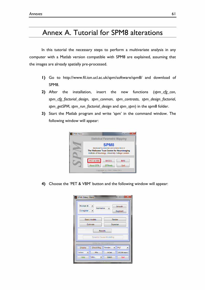
Annexes 61
Annex A. Tutorial for SPM8 alterations
In this tutorial the necessary steps to perform a multivariate analysis in any
computer with a Matlab version compatible with SPM8 are explained, assuming that
the images are already spatially pre-processed.
1) Go to http://www.fil.ion.ucl.ac.uk/spm/software/spm8/ and download of
SPM8.
2) After the installation, insert the new functions (spm_cfg_con,
spm_cfg_factorial_design, spm_conman, spm_contrasts, spm_design_factorial,
spm_getSPM, spm_run_factorial_design and spm_spm) in the spm8 folder.
3) Start the Matlab program and write ‘spm’ in the command window. The
following window will appear:
4) Choose the ‘PET & VBM’ button and the following window will appear:
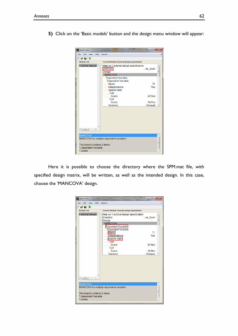
Annexes 62
5) Click on the ‘Basic models’ button and the design menu window will appear:
Here it is possible to choose the directory where the SPM.mat file, with
specified design matrix, will be written, as well as the intended design. In this case,
choose the ‘MANCOVA’ design.
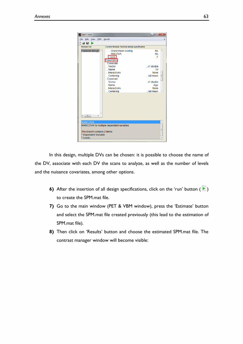
Annexes 63
In this design, multiple DVs can be chosen: it is possible to choose the name of
the DV, associate with each DV the scans to analyze, as well as the number of levels
and the nuisance covariates, among other options.
6) After the insertion of all design specifications, click on the ‘run’ button ( )
to create the SPM.mat file.
7) Go to the main window (PET & VBM window), press the ‘Estimate’ button
and select the SPM.mat file created previously (this lead to the estimation of
SPM.mat file).
8) Then click on ‘Results’ button and choose the estimated SPM.mat file. The
contrast manager window will become visible:
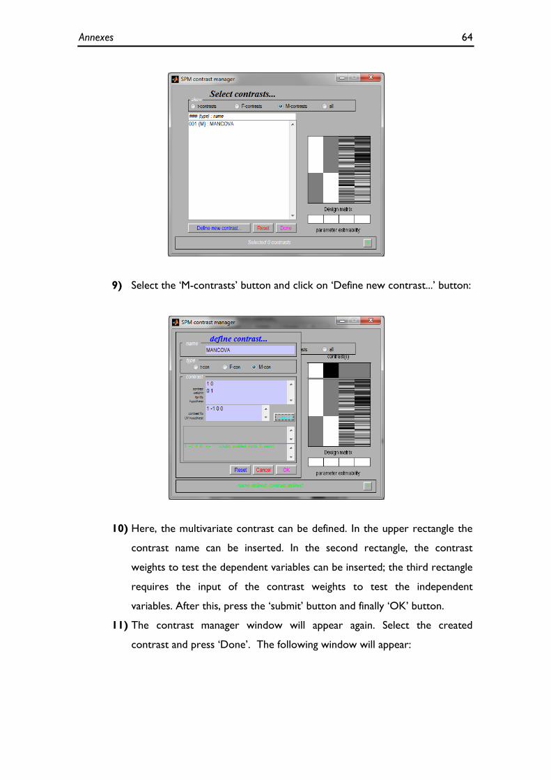
Annexes 64
9) Select the ‘M-contrasts’ button and click on ‘Define new contrast...’ button:
10) Here, the multivariate contrast can be defined. In the upper rectangle the
contrast name can be inserted. In the second rectangle, the contrast
weights to test the dependent variables can be inserted; the third rectangle
requires the input of the contrast weights to test the independent
variables. After this, press the ‘submit’ button and finally ‘OK’ button.
11) The contrast manager window will appear again. Select the created
contrast and press ‘Done’. The following window will appear:
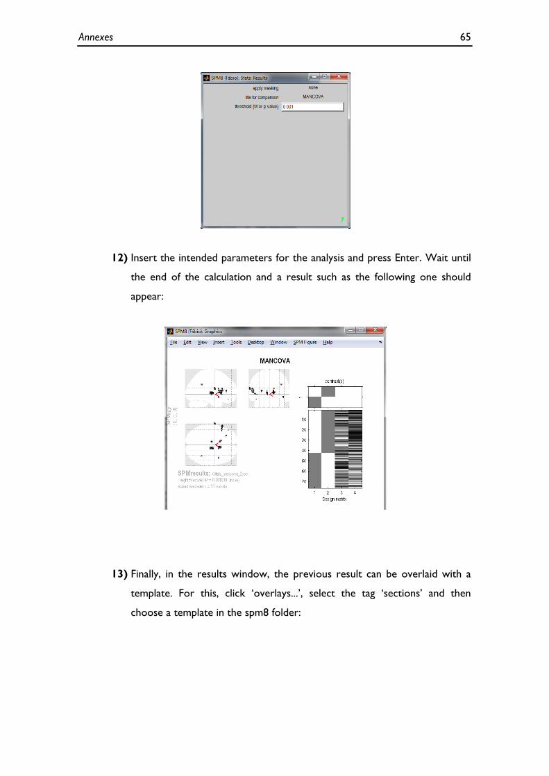
Annexes 65
12) Insert the intended parameters for the analysis and press Enter. Wait until
the end of the calculation and a result such as the following one should
appear:
13) Finally, in the results window, the previous result can be overlaid with a
template. For this, click ‘overlays...’, select the tag ‘sections’ and then
choose a template in the spm8 folder:
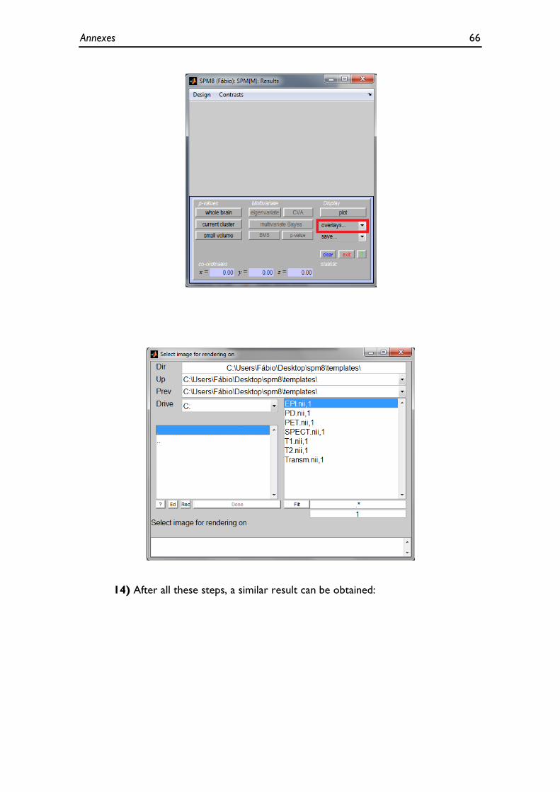
Annexes 66
14) After all these steps, a similar result can be obtained:
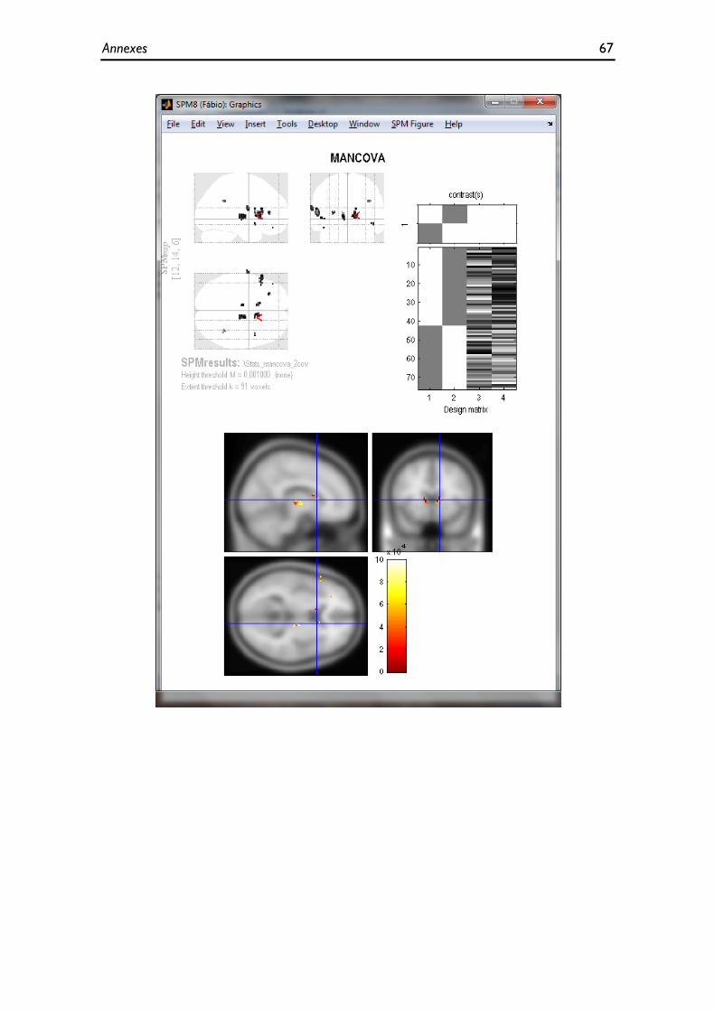
Annexes 67