fdanova: an r software package for analysis of variance

fdANOVA: An R Software Package for

Analysis of Variance for Univariate and

Multivariate Functional Data

Tomasz Gorecki

Adam Mickiewicz University Lukasz Smaga

Adam Mickiewicz University

Abstract

Functional data, i.e., observations represented by curves or functions, frequently arisein various fields. The theory and practice of statistical methods for such data is referredto as functional data analysis (FDA) which is one of major research fields in statistics.The practical use of FDA methods is made possible thanks to availability of specializedand usually free software. In particular, a number of R packages is devoted to these meth-ods. In the vignette, we introduce a new R package fdANOVA which provides an accessto a broad range of global analysis of variance methods for univariate and multivariatefunctional data. The implemented testing procedures mainly for homoscedastic case arebriefly overviewed and illustrated by examples on a well known functional data set. Toreduce the computation time, parallel implementation is developed.

Keywords: analysis of variance, functional data, fdANOVA, R.

1. Introduction

In recent years considerable attention has been devoted to analysis of so called functionaldata. The functional data are represented by functions or curves which are observations of arandom variable (or random variables) taken over a continuous interval or in large discretiza-tion of it. Sets of functional observations are peculiar examples of the high-dimensional datawhere the number of variables significantly exceeds the number of observations. Such dataare often gathered automatically due to advances in modern technology, including comput-ing environments. The functional data are naturally collected in agricultural sciences, be-havioral sciences, chemometrics, economics, medicine, meteorology, spectroscopy, and manyothers. The main purpose of functional data analysis (FDA) is to provide tools for statis-tically describing and modelling sets of functions or curves. The monographs by Ramsayand Silverman (2005), Ferraty and Vieu (2006), Horvath and Kokoszka (2012) and Zhang(2013) present a broad perspective of the FDA solutions. The following problems for func-tional data are commonly studied (see also the review papers of Cuevas 2014; Wang, Chiou,and Muller 2016): analysis of variance (Faraway 1997; Cuevas, Febrero, and Fraiman 2004;Shen and Faraway 2004; Zhang and Chen 2007; Cuesta-Albertos and Febrero-Bande 2010;Zhang 2011, 2013; Zhang and Liang 2014; Gorecki and Smaga 2015; Zhang, Cheng, Tseng,and Wu 2013), canonical correlation analysis (Krzysko and Waszak 2013; Keser and Kocakoc2015), classification (James and Hastie 2001; Delaigle and Hall 2012, 2013; Chang, Chen,

2 fdANOVA: Analysis of Variance for Functional Data in R

and Ogden 2014), cluster analysis (Giacofci, Lambert-Lacroix, Marot, and Picard 2013; Cof-fey, Hinde, and Holian 2014; Yamamoto and Terada 2014), outlier detection (Febrero-Bande,Galeano, and Gonzalez-Manteiga 2008), principal component analysis (Boente, Barrera, andTyler 2014; Fremdt, Horvath, Kokoszka, and Steinebach 2014), regression analysis (Chen,Hall, and Muller 2011; Hilgert, Mas, and Verzelen 2013; Morris 2015; Robbiano, Saumard,and Cure 2015; Peng, Zhou, and Tang 2016), repeated measures analysis (Martınez-Camblorand Corral 2011; Smaga 2017), simultaneous confidence bands (Degras 2011; Cao, Yang, andTodem 2012; Ma, Yang, and Carroll 2012). The above references concern the univariatefunctional data. However, some methods have their multivariate counterparts, e.g., analy-sis of variance (Gorecki and Smaga 2017a), canonical correlation analysis (Gorecki, Krzysko,Waszak, and Wo lynski 2016a), classification (Gorecki, Krzysko, and Wo lynski 2015; Goreckiet al. 2016a; Gorecki, Krzysko, and Wo lynski 2016b), cluster analysis (Tokushige, Yadohisa,and Inada 2007; Jacques and Preda 2014; Park and Ahn 2016), linear regression and predic-tion (Chiou, Yang, and Chen 2016; Krzysko and Smaga 2017), principal component analysis(Berrendero, Justel, and Svarc 2011; Chiou, Chen, and Yang 2014), statistical modelling(Chiou and Muller 2014). Some examples of applications of functional data analysis can befound in Ogden, Miller, Takezawa, and Ninomiya (2002), Pfeiffer, Bura, Smith, and Rut-ter (2002), Rossi, Wang, and Ramsay (2002), Jank and Shmueli (2006), Febrero-Bande et al.

(2008), Bobelyn, Serban, Nicu, Lammertyn, Nicolai, and Saeys (2010), Tarrıo-Saavedra, Naya,Francisco-Fernandez, Artiaga, and Lopez-Beceiro (2011) and Long, Li, Wang, and Cheng(2012).

Many methods for functional data analysis have been already implemented in the R software(R Core Team 2017). The packages fda (Ramsay, Hooker, and Graves 2009; Ramsay, Wick-ham, Graves, and Hooker 2014) and fda.usc (Febrero-Bande and Oviedo de la Fuente 2012)are the biggest and probably the most commonly used ones. The first package includes thetechniques for functional data in the Hilbert space L2(I) of square integrable functions over aninterval I = [a, b]. On the other hand, in the second one, many of the methods implemented donot need such assumption and use only the values of functions evaluated on a grid of discretiza-tion points (also non-equally spaced). There is also a broad range of R packages containingsolutions for more particular functional data problems: Widely used principal componentsanalysis for functional data implemented in the packages fda and fda.usc is also available infdapace (Dai, Hadjipantelis, Ji, Muller, and Wang 2016), fpca (Peng and Paul 2011), fdasrvf(Tucker 2017) and MFPCA (Happ 2017; Happ and Greven 2016) ones. For classificationand cluster analysis, the packages classiFunc (Maierhofer 2017), fdakma (Parodi, Patriarca,Sangalli, Secchi, Vantini, and Vitelli 2015), Funclustering (Soueidatt and *. 2014), funcy (Yas-souridis 2016) and GPFDA (Shi and Cheng 2014) can be used. In the packages fdaPDE (Lila,Sangalli, Ramsay, and Formaggia 2016), FDboost (Brockhaus, Scheipl, Hothorn, and Greven2015; Brockhaus and Rugamer 2016), flars (Cheng and Shi 2016), funreg (Dziak and Shiyko2016) and refund (Goldsmith, Scheipl, Huang, Wrobel, Gellar, Harezlak, McLean, Swihart,Xiao, Crainiceanu, and Reiss 2016), a lot of work was done to develop the regression analysisfor functional data. The packages freqdom (Hormann and Kidzinski 2015), ftsa (Shang 2013;Hyndman and Shang 2016), ftsspec (Tavakoli 2015) and pcdpca (Kidzinski, Jouzdani, andKokoszka 2016) provide implementation of various methods of functional time series analysis.Methods for the robust analysis of univariate and multivariate functional data are providedin the roahd package (Tarabelloni, Arribas-Gil, Ieva, Paganoni, and Romo 2017). Intervaltesting procedures for functional data in different frameworks (i.e., one or two-population

Tomasz Gorecki, Lukasz Smaga 3

frameworks, functional linear models) are implemented in the fdatest package (Pini and Van-tini 2015). The functional data analysis in mixed model framework is implemented in thepackage fdaMixed (Markussen 2014). The functional observations can be visualized by manyof plots implemented in the following packages GOplot (Walter, Sanchez-Cabo, and Ricote2015), rainbow (Shang and Hyndman 2016) and refund.shiny (Wrobel and Goldsmith 2016).The packages fds (Shang and Hyndman 2013) and mfds (Gorecki and Smaga 2017b) containsome interesting functional data sets.

Despite so many R packages for functional data analysis, a broad range of test for a widelyapplicable analysis of variance problem for functional data was implemented very recentlyin the package fdANOVA. Earlier, only the testing procedures of Cuevas et al. (2004) andCuesta-Albertos and Febrero-Bande (2010) were available in the package fda.usc. The pack-age fdANOVA is available from the Comprehensive R Archive Network at http://CRAN.

R-project.org/package=fdANOVA. It is the aim of this package to provide a few functionsimplementing most of known analysis of variance tests for univariate and multivariate func-tional data, mainly for homoscedastic case. Most of them are based on bootstrap, permuta-tions or projections, which may be time-consuming. For this reason, the package also containsparallel implementations which enable to reduce the computation time significantly, which isshown in empirical evaluation.

The rest of the vignette is organized in the following manner. In Section 2, the problemsof the analysis of variance for univariate and multivariate functional data are introduced. Areview of most of the known solutions of these problems is also presented there. Some of thetesting procedures are slightly generalized. Since it was not easy task to implement manydifferent tests in a few functions, their usage may also be not easy at first. Thus, Section 3contains a detailed description of (eventual) preparation of data and package functionality aswell as a package demonstration on commonly used real data set.

2. Analysis of variance for functional data

In this section, we briefly describe most of the known testing procedures for the analysis ofvariance problem for functional data in the univariate and multivariate cases. All of them areimplemented in the package fdANOVA.

2.1. Univariate case

We consider the l groups of independent random functions Xij(t), i = 1, . . . , l, j = 1, . . . , ni

defined over a closed and bounded interval I = [a, b]. Let n = n1+ · · ·+nl. These groups maydiffer in mean functions, i.e., we assume that Xij(t), j = 1, . . . , ni are stochastic processeswith mean function µi(t), t ∈ I and covariance function γ(s, t), s, t ∈ I, for i = 1, . . . , l. Ofinterest is to test the following null hypothesis

H0 : µ1(t) = · · · = µl(t), t ∈ I. (1)

The alternative is the negation of the null hypothesis. The problem of testing this hypothesisis known as the one-way analysis of variance problem for functional data (FANOVA).

Many of the tests for (1) are based on the pointwise F test statistic (Ramsay and Silverman

http://CRAN.R-project.org/package=fdANOVA

http://CRAN.R-project.org/package=fdANOVA


2005) given by the formula

Fn(t) =SSRn(t)/(l − 1)

SSEn(t)/(n− l),

where

SSRn(t) =l

∑

i=1

ni(Xi(t) − X(t))2, SSEn(t) =l

∑

i=1

ni∑

j=1

(Xij(t) − Xi(t))2

are the pointwise between-subject and within-subject variations respectively, and X(t) =(1/n)

∑li=1

∑ni

j=1Xij(t) and Xi(t) = (1/ni)∑ni

j=1Xij(t), i = 1, . . . , l, are respectively thesample grand mean function and the sample group mean functions.

Faraway (1997) and Zhang and Chen (2007) proposed to use only the pointwise between-subject variation and considered the test statistic

∫

I SSRn(t)dt. Tests based on it are calledthe L2-norm-based tests. The distribution of this test statistic can be approximated by thatof βχ2

d and comparing the first two moments of these random variables. The parameters βand d were estimated by the naive and biased-reduced methods (see, for instance, Goreckiand Smaga 2015, for more detail). Thus we have the L2-norm-based tests with the naive andbiased-reduced methods of estimation of these parameters (the L2N and L2B tests for short).In case of non-Gaussian samples or small sample sizes, the bootstrap L2-norm-based test isalso considered (the L2b tests for short).

A bit different L2-norm-based test was proposed by Cuevas et al. (2004). Namely, theyconsidered

∑

1≤i<j≤l ni

∫

I(Xi(t) − Xj(t))2dt as a test statistic and approximated its null dis-

tribution by a parametric bootstrap method via re-sampling the Gaussian processes involvedin the limit random expression of their test statistic under H0. Cuevas et al. (2004) inves-tigated two testing procedures (the CH and CS tests for short) under homoscedastic andheteroscedastic cases. The tests differ in estimating the covariance functions.

Following test, which uses both the pointwise between-subject and within-subject variations,is known as the F -type test. More precisely, the test statistic is of the form

∫

I SSRn(t)dt/(l − 1)∫

I SSEn(t)dt/(n− l). (2)

Tests of this type were considered by Shen and Faraway (2004) and Zhang (2011). Thenull distribution of the above test statistic is approximated by F(l−1)κ,(n−l)κ distribution anddepending on the method of estimation of parameter κ, the F -type tests based on naive andbiased-reduced methods of estimation are considered (the FN and FB tests for short). For thesame reasons as for L2-norm-based test, the Fb test is also investigated, i.e., the bootstrapF -type test.

The following testing procedure, which also uses the test statistic (2), is the slightly mod-ified procedure proposed by Gorecki and Smaga (2015). Assume that Xij ∈ L2(I), i =1, . . . , l, j = 1, . . . , ni, where L2(I) is a Hilbert space consisting of square integrable functionson I, equipped with the inner product of the form 〈f, g〉 =

∫

I f(t)g(t)dt. We represent thefunctional observations by a finite number of basis functions ϕm ∈ L2(I),m = 1, . . . , i.e.,

Xij(t) ≈

K∑

m=1

cijmϕm(t), t ∈ I, (3)


where cijm, m = 1, . . . ,K, are random variables such that Var(cijm) < ∞ and K is sufficientlylarge (see Ramsay and Silverman 2005, for more details about basis function representation).By the results of Gorecki et al. (2015), the commonly used least squares method (see, forexample, Krzysko and Waszak 2013) seems to be one of the best for estimation of coefficientscijm, so we use only that method for this purpose. The value of K can be selected for eachobservation Xij(t) using certain information criterion, e.g., BIC, eBIC, AIC or AICc. Fromthe values of K corresponding to all observations a modal, minimum, maximum or mean valueis selected as the common value for all processes Xij(t). By using (3) and easy modificationsof the results obtained by Gorecki and Smaga (2015), we proved that the test statistic (2) isapproximately equal to

(a− b)/(l − 1)

(c− a)/(n− l), (4)

where

a =l

∑

i=1

1

ni1⊤ni

C⊤i JϕCi1ni

, b =1

n

l∑

i=1

l∑

j=1

1⊤niC⊤

i JϕCj1nj, c =

l∑

i=1

trace(C⊤i JϕCi),

1a is the a× 1 vector of ones, Ci = (cijm)j=1,...,ni;m=1,...,K are K × ni matrices of coefficients,i = 1, . . . , l, and Jϕ :=

∫

I ϕ(t)ϕ⊤(t)dt is the K ×K cross product matrix corresponding tothe vector ϕ(t) = (ϕ1(t), . . . , ϕK(t))⊤. So the statistic (2) can be calculated based only onthe coefficients cijm and the matrix Jϕ, which can be approximated by using the functioninprod() from the R package fda (Ramsay et al. 2009, 2014) (For orthonormal basis, Jϕ isthe identity matrix.). Moreover, observe that any permutation of the observations leaves thevalues of the sums b and c unchanged. For this reason, Gorecki and Smaga (2015) consideredthe permutation test based on (4). We refer to this test as the FP test. Simulation studies ofGorecki and Smaga (2015) suggest that the FP test has better finite sample properties thanthe F -type and L2-norm-based tests. Moreover, for short functional data (i.e., observed ona short grid of design time points) it may also be better than the GPF test described in thefollowing paragraph.

In the above test statistics, SSRn(t) and SSEn(t) were integrated separately. However, by thesimulation results of Gorecki and Smaga (2015), it follows that for example integrating thewhole quotient SSRn(t)/SSEn(t) is more powerful in many situations. Such test statistic ofthe form

∫

I Fn(t)dt was considered by Zhang and Liang (2014). They proposed the globalizingpointwise F test (the GPF test) based on this test statistic and critical value approximatedsimilarly as for the L2-norm-based test. Although integration seems to be a natural operationon Fn(t) or its part, in some situations other using of Fn(t) may be better in the sense ofpower, as was shown by Zhang et al. (2013). Instead of integral of Fn(t), they used simplysupt∈I Fn(t) as a test statistic and simulated the critical value of the resulting Fmaxb test viabootstrapping. By intensive simulation studies, Zhang et al. (2013) found that the Fmaxb(resp. GPF) test generally has higher power than the GPF (resp. Fmaxb) test when thefunctional data are moderately or highly (resp. less) correlated.

A different approach to test the null hypothesis (1) was proposed by Cuesta-Albertos andFebrero-Bande (2010). Their tests are based on the analysis of randomly chosen projections.Suppose that µi, i = 1, . . . , l belong to a separable Hilbert space H endowed with a scalarproduct 〈·, ·〉, and ξ is a Gaussian distribution on this space and each of its one-dimensionalprojections is nondegenerate. Let h be a vector chosen randomly from H using the distribution


ξ. When the null hypothesis H0 holds, then we can easily observe that for every h ∈ H, thefollowing null hypothesis

Hh0 : 〈µ1, h〉 = · · · = 〈µl, h〉 (5)

also holds. Moreover, Cuesta-Albertos and Febrero-Bande (2010) showed that for ξ-almostevery h, Hh

0 fails, in case of failing of H0. Therefore, a testing procedure for Hh0 can be

used to test H0. Assuming that Xij ∈ L2(I), i = 1, . . . , l, j = 1, . . . , ni, Cuesta-Albertos andFebrero-Bande (2010) propose the following testing procedure, in which k random projectionsare used:

1. Choose, with Gaussian distribution, functions hr ∈ L2(I), r = 1, . . . , k.

2. Compute the projections P rij =

∫

I Xij(t)hr(t)dt/(∫

I h2r(t)dt

)1/2for i = 1, . . . , l, j =

1, . . . , ni, r = 1, . . . , k.

3. For each r ∈ {1, . . . , k}, apply the appropriate ANOVA test for P rij , i = 1, . . . , l, j =

1, . . . , ni. Let p1, . . . , pk denote the resulting p values.

4. Compute the final p value for H0 by the formula inf{kp(r)/r, r = 1, . . . , k}, wherep(1) ≤ · · · ≤ p(k) are the ordered p values obtained in step 3.

The tests based on the above procedure are referred to as the test based on random projections.Cuesta-Albertos and Febrero-Bande (2010) suggested to use k near 30, which was confirmedby the results of Gorecki and Smaga (2017a). However, in the case of unconvincing results ofthe test, we should use a higher number of projections. We also have to choose a Gaussiandistribution and ANOVA test appearing in steps 1 and 3 of the above procedure, respectively.We can do this in many ways and some of them are implemented in the package fdANOVA

(see Section 3). In step 4, we can also use other final p values instead of Benjamini andHochberg procedure (Benjamini and Hochberg 1995; Benjamini and Yekutieli 2001), as forexample Bonferroni correction. However, according to our experience, the test with correctedp value given in step 4 behaves best under finite samples, so we use only it. The procedure byCuesta-Albertos and Febrero-Bande (2010) can also handle the heteroskedastic case. It onlydepends that such procedure exists for the projected data.

2.2. Multivariate case

Now, we study the multivariate version of the ANOVA problem for functional data as wellas extensions of certain methods presented in the last section to this problem. The results ofthis section were mainly obtained by Gorecki and Smaga (2017a).

Instead of single functions, we consider independent vectors of random functions Xij(t) =(Xij1(t), . . . , Xijp(t))

⊤ ∈ SPp(µi,Γ), i = 1, . . . , l, j = 1, . . . , ni defined over the interval I,where SPp(µ,Γ) is a set of p-dimensional stochastic processes with mean vector µ(t), t ∈ Iand covariance function Γ(s, t), s, t ∈ I. In the multivariate analysis of variance problem forfunctional data (FMANOVA), we have to test the null hypothesis as follows:

H0 : µ1(t) = · · · = µl(t), t ∈ I. (6)

The first (permutation) tests are based on a basis function representation of the components ofthe vectors Xij(t), i = 1, . . . , l, j = 1, . . . , ni, similarly as in the FP test. For this purpose, we


assume that Xij belong to Lp2(I) – a Hilbert space of p-dimensional vectors of square integrable

functions on the interval I, equipped with the inner product: 〈x,y〉 =∫

I x⊤(t)y(t)dt. Hence

we can represent the components of Xij(t) in a similar way as in (3). Then the vectors arerepresented as follows

Xij(t) ≈

cij1...

cijp

ϕ(t) = cijϕ(t), (7)

where cijm = (cijm1, . . . , cijmKm, 0, . . . , 0) ∈ RKM , ϕ(t) = (ϕ1(t), . . . , ϕKM (t))⊤, t ∈ I and

i = 1, . . . , l, j = 1, . . . , ni, m = 1, . . . , p, KM = max{K1, . . . ,Kp}. The coefficients in cijand values of Km are estimated separately for each feature by using the same methods asdescribed in Section 2.1. Similarly to MANOVA (see Anderson 2003), the following matriceswere used in constructing test statistics for FMANOVA problem:

E =l

∑

i=1

ni∑

j=1

∫

I

(

Xij(t) − Xi(t)) (

Xij(t) − Xi(t))⊤

dt,

H =l

∑

i=1

ni

∫

I

(

Xi(t) − X(t)) (

Xi(t) − X(t))⊤

dt,

where Xi(t) = (1/ni)∑ni

j=1Xij(t), i = 1, . . . , l and X(t) = (1/n)∑l

i=1

∑ni

j=1Xij(t), t ∈ I.Modifying the results of Gorecki and Smaga (2017a), we showed that these matrices can bedesignated only by the coefficient matrices cij and appropriate cross product matrix, i.e.,E ≈ A−B and H ≈ B−C, where

A =

l∑

i=1

ni∑

j=1

cijJϕc⊤ij , B =

l∑

i=1

1

ni

ni∑

j=1

ni∑

m=1

cijJϕc⊤im, C =1

n

l∑

i=1

ni∑

j=1

l∑

t=1

nt∑

u=1

cijJϕc⊤tu,

and Jϕ is the KM × KM cross product matrix corresponding to ϕ. The following teststatistics for (6) are constructed based on those appearing in MANOVA (Anderson 2003):the Wilk’s lambda W = det(E)/ det(E + H), the Lawley-Hotelling trace LH = trace(HE−1),the Pillai trace P = trace(H(H + E)−1), the Roy’s maximum root R = λmax(HE−1), whereλmax(M) is the maximum eigenvalue of a matrix M. We consider the permutation testingprocedures based on these test statistics and refer to them as the W, LH, P and R tests,respectively. Generally, we refer to them as the permutation tests based on a basis functionrepresentation for the FMANOVA problem. A quite fast implementation of these permu-tation tests was obtained by observing that the matrices A and C are not changed by anypermutation of the data.

The second group of testing procedures for (6) is based on random projections similarly asin the FANOVA test based on random projections. Let a space H and a distribution ξbe defined as in Section 2.1. Assume that µij ∈ H, where µij are the components of thevectors µi, i = 1, . . . , l, j = 1, . . . , p. If the null hypothesis in (6) holds, then for everyH = (h1, . . . , hp)

⊤ ∈ H × · · · × H,

HH

0 : (〈µ11, h1〉, . . . , 〈µ1p, hp〉)⊤ = · · · = (〈µl1, h1〉, . . . , 〈µlp, hp〉)

⊤ (8)

also holds, and further when H0 fails, for (ξ × · · · × ξ)-almost every H ∈ H × · · · × H, HH

0

also fails (see Theorem 2.2 in Gorecki and Smaga 2017a). Thus, a test for the MANOVA


problem can be used to test the FMANOVA one by using it to test the null hypothesis (8).For this reason, Gorecki and Smaga (2017a) investigated the similar testing procedure basedon k random projection as described in Section 2.1, which the first three steps are now asfollows:

1. Choose, with Gaussian distribution, functions hmr ∈ L2(I), m = 1, . . . , p, r = 1, . . . , k.

2. Compute the projections P rijm =

∫

I Xijm(t)hmr(t)dt/(∫

I h2mr(t)dt

)1/2for i = 1, . . . , l,

j = 1, . . . , ni, m = 1, . . . , p, r = 1, . . . , k.

3. For each r ∈ {1, . . . , k}, apply the appropriate MANOVA test for Prij = (P r

ij1, . . . , Prijp)

⊤,i = 1, . . . , l, j = 1, . . . , ni. Let p1, . . . , pk denote the resulting p values.

In step 3 of this procedure, the well-known MANOVA tests were applied, namely Wilk’slambda test (Wp test), the Lawley-Hotelling trace test (LHp test), the Pillai trace test (Pptest) and Roy’s maximum root test (Rp test). Their permutation versions are also investi-gated.

By the extensive Monte Carlo simulation studies of Gorecki and Smaga (2017a), the perfor-mance of the tests considered except the Rp test is very satisfactory under finite samples.Unfortunately, the Rp test does not control the nominal type-I error level, and hence it cannot be recommended. The other testing procedures do not perform equally well, and there isno single method performing best.

3. R implementation

In this section, we present the R package fdANOVA and illustrate the usage of it step by stepusing certain real data set. First, however, we mention about the eventual preparation of thefunctional data in the R program to use the functions of our package properly.

3.1. Preparation of the data

In practice, functional samples are not continuously observed, i.e., each function is usuallyobserved on a grid of design time points. In our implementations of FANOVA and FMANOVAtests in the R programming language, all functions are observed on a common grid of designtime points equally spaced in the interval I = [a, b]. In the case where the design timepoints are different for different individual functions or not equally spaced in I, we follow themethodology proposed by Zhang (2013). First, we have to reconstruct the functional samplesfrom the observed discrete functional samples using smoothing technique such as regressionsplines, smoothing splines, P-splines or local polynomial smoothing (see Zhang 2013, Chapters2-3). For this purpose, in R we can use the function smooth.spline() from the stats package(R Core Team 2017) or functions given in the packages splines (R Core Team 2017), bigsplines(Helwig 2016), pspline (S original by Jim Ramsey. R port by Brian Ripley 2015) and locpol

(Ojeda Cabrera 2012). After that we discretize each individual function of the reconstructedfunctional samples on a common grid of T time points equally spaced in I, and then theimplementations of the tests can be applied to discretized samples.

3.2. Package functionality


Now, we describe the implementation of the tests for analysis of variance problem for univari-ate and multivariate functional data in the R package fdANOVA. As we will see many of theimplemented tests may be performed with different values of parameters. However, by simu-lation and real data examples presented in the previous papers (see Sections 2), satisfactoryresults are usually obtained by using the default values of these parameters. Nevertheless,when the results are unconvincing (e.g., the p values are close to the significance level), wehave the opportunity to use other options provided by the functions of the package.

All tests for FANOVA problem presented in Section 2.1 are implemented in the functionfanova.tests():

R> library("fdANOVA")

R> str(fanova.tests)

function(x = NULL, group.label, test = "ALL", params = NULL,

parallel = FALSE, nslaves = NULL)

which is controlled by the following parameters:

❼ x – a T ×n matrix of data, whose each column is a discretized version of a function androws correspond to design time points. Its default values is NULL, since if the FP testis only used, we can give a basis representation of the data instead of raw observations(see the list paramFP below). For any of the other testing procedures, the raw data areneeded.

❼ group.label – a vector containing group labels.

❼ test – a kind of indicator which establishes a choice of FANOVA tests to be performed.Its default value means that all testing procedures of Section 2.1 will be used. Whenwe want to use only some tests, the parameter test is an appropriate subvector of thefollowing vector of tests’ labels (see Section 2.1):

c("FP", "CH", "CS", "L2N", "L2B", "L2b", "FN", "FB", "Fb", "GPF",

"Fmaxb", "TRP")

❼ params – a list of additional parameters for the FP, CH, CS, L2b, Fb, Fmaxb tests andthe test based on random projections. Its possible elements and their default valuesare described below. The default value of this parameter means that these tests areperformed with their default values.

❼ parallel – a logical indicating whether to use parallelization.

❼ nslaves – if parallel = TRUE, a number of slaves. Its default value means that it willbe equal to a number of logical processes of a computer used.

The list params can contain all or a part of the elements paramFP, paramCH, paramCS,paramL2b, paramFb, paramFmaxb and paramTRP for passing the parameters for the FP, CH,CS, L2b, Fb, Fmaxb tests and the test based on random projections, respectively, to thefunction fanova.tests(). They are described as follows. The list


paramFP = list(int, B.FP = 1000, basis = c("Fourier", "b-spline", "own"),

own.basis, own.cross.prod.mat,

criterion = c("BIC", "eBIC", "AIC", "AICc", "NO"),

commonK = c("mode", "min", "max", "mean"),

minK = NULL, maxK = NULL, norder = 4, gamma.eBIC = 0.5)

contains the parameters of the FP test and their default values, where:

❼ int – a vector of two elements representing the interval I = [a, b]. When it is notspecified, it is determined by a number of design time points.

❼ B.FP – a number of permutation replicates.

❼ basis – a choice of basis of functions used in the basis function representation of thedata.

❼ own.basis – if basis = "own", a K×n matrix with columns containing the coefficientsof the basis function representation of the observations.

❼ own.cross.prod.mat – if basis = "own", a K×K cross product matrix correspondingto a basis used to obtain the matrix own.basis.

❼ criterion – a choice of information criterion for selecting the optimum value of K.criterion = "NO" means that K is equal to the parameter maxK defined below. By(3), we have BIC(Xij) = T log(e⊤ijeij/T ) + K log T , eBIC(Xij) = T log(e⊤ijeij/T ) +

K[log T +2γ log(Kmax)], AIC(Xij) = T log(e⊤ijeij/T )+2K and AICc(Xij) = AIC(Xij)+

2K(K+1)/(n−K−1), where eij = (eij1, . . . , eijT )⊤, eijr = Xij(tr)−∑K

m=1 cijmϕm(tr),t1, . . . , tT are the design time points, γ ∈ [0, 1], Kmax is a maximum K considered andlog denotes the natural logarithm.

❼ commonK – a choice of method for selecting the common value for all observations fromthe values of K corresponding to all processes.

❼ minK (resp. maxK) – a minimum (resp. maximum) value of K. When basis =

"Fourier", they have to be odd numbers. If minK = NULL and maxK = NULL, wetake minK = 3 and maxK equal to the largest odd number smaller than the number ofdesign time points. If maxK is greater than or equal to the number of design time points,maxK is taken as above. For basis = "b-spline", minK (resp. maxK) has to be greater(resp. smaller) than or equal to norder defined below (resp. T ). If minK = NULL orminK < norder and maxK = NULL or maxK > T , then we take minK = norder andmaxK = T .

❼ norder – if basis = "b-spline", an integer specifying the order of b-splines.

❼ gamma.eBIC – a γ ∈ [0, 1] parameter in the eBIC.

It should be noted that the AICc may choose the finale model with a number K of coefficientsclose to a number of observations n, when Kmax is greater than n. Such selection usuallydiffers from choices suggested by other criterion, but it seems that this does not have muchimpact on the results of testing.


For the CH and CS (resp. L2b, Fb and Fmaxb) tests, the parameters paramCH and paramCS

(resp. paramL2b, paramFb and paramFmaxb) denote the numbers of discretized artificial tra-jectories for certain Gaussian processes (resp. bootstrap samples) used to approximate thenull distributions of their test statistics. The default value of each of these parameters is10,000. The parameters of the test based on random projections and their default values arecontained in a list

paramTRP = list(k = 30, projection = c("GAUSS", "BM"),

permutation = FALSE, B.TRP = 10000,

independent.projection.tests = TRUE)

where:

❼ k – a vector of numbers of projections.

❼ projection – a method of generating Gaussian processes in step 1 of the testing pro-cedure based on random projections presented in Section 2. If projection = "GAUSS",the Gaussian white noise is generated as in the function anova.RPm() from the R pack-age fda.usc (Febrero-Bande and Oviedo de la Fuente 2012). In the second case, theBrownian motion is generated.

❼ permutation – a logical indicating whether to compute p values by permutation method.

❼ B.TRP – a number of permutation replicates.

❼ independent.projection.tests – a logical indicating whether to generate the randomprojections independently or dependently for different elements of vector k. In the firstcase, the random projections for each element of vector k are generated separately, whilein the second one, they are generated as chained subsets, e.g., for k = c(5, 10), thefirst 5 projections are a subset of the last 10. The second way of generating randomprojections is faster than the first one.

A Brownian process in [a, b] has small variances near a and higher variances close to b. Thismeans that the tests based on random projections and the Brownian motion may be moreable to detect differences among mean groups, when those differences are much closer to bthan to a.

To perform step 3 of the procedure based on random projections given in Section 2.1, in thepackage, we use five testing procedures: the standard (paramTRP$permutation = FALSE) andpermutation (paramTRP$permutation = TRUE) tests based on ANOVA F test statistic andANOVA-type statistic (ATS) proposed by Brunner, Dette, and Munk (1997), as well as thetesting procedure based on Wald-type permutation statistic (WTPS) of Pauly, Brunner, andKonietschke (2015).

The function fanova.tests() returns a list of the class fanovatests. This list contains thevalues of the test statistics, the p values and the parameters used. The results for a given testare given in a list (being an element of output list) named the same as the indicator of a testin the vector test. Additional outputs as the chosen optimal length of basis expansion (theFP test), the values of estimators used in approximations of null distributions of test statistics(the L2N, L2B, FN, FB, GPF tests) and projections of the data (the test based on random


projections) are contained in appropriate lists. If independent.projection.tests = TRUE,the projections of the data are contained in a list of the length equal to length of vector k,whose i-th element is an n× k[i] matrix with columns being projections of the data. Whenindependent.projection.tests = FALSE, the projections of the data are contained in ann× max(k) matrix with columns being projections of the data.

The permutation tests based on a basis function representation for FMANOVA problem, i.e.,the W, LH, P and R tests are implemented in the function fmanova.ptbfr():


R> str(fmanova.ptbfr)

function(x = NULL, group.label, int, B = 1000,

parallel = FALSE, nslaves = NULL,

basis = c("Fourier", "b-spline", "own"),

own.basis, own.cross.prod.mat,

criterion = c("BIC", "eBIC", "AIC", "AICc", "NO"),

commonK = c("mode", "min", "max", "mean"),

minK = NULL, maxK = NULL, norder = 4, gamma.eBIC = 0.5)

The parameters group.label, int, B, parallel, nslaves, basis, norder and gamma.eBIC

are the same as in the function fanova.tests() (B corresponds to B.FP). The other argumentsof fmanova.ptbfr() are described as follows:

❼ x – a list of T × n matrices of data, whose each column is a discretized version ofa function and rows correspond to design time points. The mth element of this listcontains the data of mth feature, m = 1, . . . , p. Its default values is NULL, becausea basis representation of the data can be given instead of raw observations (see theparameter own.basis below).

❼ own.basis – if basis = "own", a list of length p, whose elements are Km × n matrices(m = 1, . . . , p) with columns containing the coefficients of the basis function represen-tation of the observations.

❼ own.cross.prod.mat – if basis = "own", a KM × KM cross product matrix corre-sponding to a basis used to obtain the list own.basis.

❼ criterion – a choice of information criterion for selecting the optimum value of Km,m = 1, . . . , p. criterion = "NO" means that Km are equal to the parameter maxK

defined below.

❼ commonK – a choice of method for selecting the common value for all observations fromthe values of Km corresponding to all processes.

❼ minK (resp. maxK) – a minimum (resp. maximum) value of Km. Further remarks aboutthese arguments are the same as for the function fanova.tests().

The function fmanova.ptbfr() returns a list of the class fmanovaptbfr containing the valuesof the test statistics (W, LH, P, R), the p values (pvalueW, pvalueLH, pvalueP, pvalueR), chosen


optimal values of Km and the parameters used. This function uses the R package fda (Ramsayet al. 2014).

The function fmanova.trp() performs the testing procedures based on random projectionsfor FMANOVA problem (the Wp, LHp, Pp and Rp tests):


R> str(fmanova.trp)

function(x, group.label, k = 30, projection = c("GAUSS", "BM"),

permutation = FALSE, B = 1000,

independent.projection.tests = TRUE,

parallel = FALSE, nslaves = NULL)

The first two parameters of this function as well as the arguments parallel, nslaves arethe same as in the function fmanova.ptbfr(). The other ones have the same meaning as inthe parameter list paramTRP of the function fanova.tests() (B corresponds to B.TRP). Thefunction fmanova.trp() returns a list of class fmanovatrp containing the parameters and thefollowing elements (|k| denotes the length of vector k): pvalues – a 4×|k| matrix of p values ofthe tests; data.projections – if independent.projection.tests = TRUE, a list of length|k|, whose elements are lists of n× p matrices of projections of the observations, while whenindependent.projection.tests = FALSE, a list of length max(k), whose elements are n×pmatrices of projections of the observations.

The executions of selecting the optimum length of basis expansion by some information cri-terion, the bootstrap, permutation and projection loops are the most time consuming stepsof the testing procedures under consideration. To reduce the computational cost of the pro-cedures, they are parallelized, when the parameter parallel is set to TRUE. The parallelexecution is handled by doParallel package (Revolution Analytics and Weston 2015).

In the package, the number of auxiliary functions are also contained. The p values of the testsbased on random projections for FANOVA problem against the number of projections arevisualized by the function plot.fanovatests() using the package ggplot2 (Wickham 2009),which is controlled by the following parameters: x – an fanovatests object, more precisely,a result of the function fanova.tests() for the standard tests based on random projections;y – an fanovatests object, more precisely, a result of the function fanova.tests() for thepermutation tests based on random projections. Similarly, the p values of the Wp, LHp,Pp and Rp tests are plotted by the function plot.fmanovatrp(). The arguments of thisfunction are as follows: x – an fmanovatrp object, more precisely, a result of the functionfmanova.trp() for the standard tests; y – an fmanovatrp object, more precisely, a resultof the function fmanova.trp() for the permutation tests; withoutRoy – a logical indicatingwhether to plot the p values of the Rp test. We can use only one of the arguments x and y,or both simultaneously.

Using the package ggplot2 (Wickham 2009), the function plotFANOVA():


R> str(plotFANOVA)

function(x, group.label = NULL, int = NULL, separately = FALSE,

means = FALSE, smooth = FALSE, ...)


produces a plot showing univariate functional observations with or without indication ofgroups as well as mean functions of samples. The following parameters control this function:

❼ x – a T ×n matrix of data, whose each column is a discretized version of a function androws correspond to design time points.

❼ group.label – a character vector containing group labels. Its default value means thatall functional observations are drawn without division into groups.

❼ int – this parameter is the same as in the function fanova.tests().

❼ separately – a logical indicating how groups are drawn. If separately = FALSE,groups are drawn on one plot by different colors. When separately = TRUE, they aredepicted in different panels.

❼ means – a logical indicating whether to plot only group mean functions.

❼ smooth – a logical indicating whether to plot reconstructed data via smoothing splinesinstead of raw data.

The functions print.fanovatests(), print.fmanovaptbfr() and print.fmanovatrp() printout the p values and values of the test statistics for the implemented testing procedures. Addi-tionally, the functions summary.fanovatests(), summary.fmanovaptbfr() and summary.fmanovatrp()

print out information about the data and parameters of the methods.

When calling the functions of the fdANOVA package, the software will check for presence ofthe doBy, doParallel, ggplot2, fda, foreach, magic, MASS and parallel packages if necessary(Hojsgaard and Halekoh 2016; Revolution Analytics and Weston 2015; Wickham 2009; Ram-say et al. 2014; Hankin 2005; Venables and Ripley 2002). If the required packages are notinstalled, an error message will be displayed.

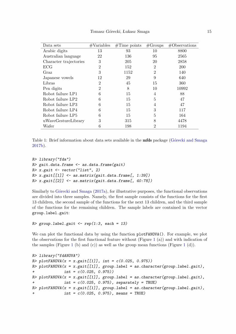
It is worth to mention that fifteen labeled multivariate functional data sets are available in themfds package (Gorecki and Smaga 2017b), which is a kind of supplement to the fdANOVA

package. Table 1 depicts brief information about these data sets, i.e., numbers of variables,design time points, groups and observations. The data sets were created from multivariatetime series data available in Chen, Keogh, Hu, Begum, Bagnall, Mueen, and Batista (2015),Leeb, Lee, Keinrath, Scherer, Bischof, and Pfurtscheller (2007), Lichman (2013) and Olszewski(2001) by extending all variables to the same length as in Rodriguez, Alonso, and Maestro(2005). They originate from different domains, including handwriting recognition, medicine,robotics, etc. The data sets can be used for illustrating and evaluating practical efficiencyof classification and statistical inference methods, etc. (see, for example, Gorecki and Smaga2015, 2017a).

3.3. Package demonstration on real data example

In this section, we provide examples that illustrate how the functions of the R packagefdANOVA can be used to analyze real data. For this purpose, we use the popular gait dataset available in the fda package. This data set consists of the angles formed by the hip andknee of each of 39 children over each child’s gait cycle. The simultaneous variations of the hipand knee angles for children are observed at 20 equally spaced time points in [0.025, 0.975].So, in this data set, we have two functional features, which we put in the list x.gait of lengthtwo, as presented below.


Data sets #Variables #Time points #Groups #Observations

Arabic digits 13 93 10 8800Australian language 22 136 95 2565Character trajectories 3 205 20 2858ECG 2 152 2 200Graz 3 1152 2 140Japanese vowels 12 29 9 640Libras 2 45 15 360Pen digits 2 8 10 10992Robot failure LP1 6 15 4 88Robot failure LP2 6 15 5 47Robot failure LP3 6 15 4 47Robot failure LP4 6 15 3 117Robot failure LP5 6 15 5 164uWaveGestureLibrary 3 315 8 4478Wafer 6 198 2 1194

Table 1: Brief information about data sets available in the mfds package (Gorecki and Smaga2017b).

R> library("fda")

R> gait.data.frame <- as.data.frame(gait)

R> x.gait <- vector("list", 2)

R> x.gait[[1]] <- as.matrix(gait.data.frame[, 1:39])

R> x.gait[[2]] <- as.matrix(gait.data.frame[, 40:78])

Similarly to Gorecki and Smaga (2017a), for illustrative purposes, the functional observationsare divided into three samples. Namely, the first sample consists of the functions for the first13 children, the second sample of the functions for the next 13 children, and the third sampleof the functions for the remaining children. The sample labels are contained in the vectorgroup.label.gait:

R> group.label.gait <- rep(1:3, each = 13)

We can plot the functional data by using the function plotFANOVA(). For example, we plotthe observations for the first functional feature without (Figure 1 (a)) and with indication ofthe samples (Figure 1 (b) and (c)) as well as the group mean functions (Figure 1 (d)).


R> plotFANOVA(x = x.gait[[1]], int = c(0.025, 0.975))

R> plotFANOVA(x = x.gait[[1]], group.label = as.character(group.label.gait),

+ int = c(0.025, 0.975))


+ int = c(0.025, 0.975), separately = TRUE)


+ int = c(0.025, 0.975), means = TRUE)


0

10

20

30

40

50

0.00 0.25 0.50 0.75 1.00

t

group.label

1

2

3

0

20

40

60

0.00 0.25 0.50 0.75 1.00

t

(a)

0

20

40

60

0.00 0.25 0.50 0.75 1.00

t

group.label

1

2

3

(b)

12

30.00 0.25 0.50 0.75 1.00

0

20

40

60

0

20

40

60

0

20

40

60

t

(c)

0

10

20

30

40

50

0.00 0.25 0.50 0.75 1.00

t

group.label

1

2

3

(d)

Figure 1: The first functional feature of the gait data without (Panel (a)) and with indicationof the samples (Panels (b) and (c)). Panel (d) depicts the group mean functions.

From Figure 1, it seems that the mean functions of the three samples do not differ significantly.To confirm this statistically, we use the FANOVA tests implemented in the fanova.tests()

function. First, we use default values of the parameters of this function:

R> set.seed(123)

R> (fanova <- fanova.tests(x = x.gait[[1]], group.label = group.label.gait))

Analysis of Variance for Functional Data

FP test - permutation test based on a basis function representation

Test statistic = 1.468218 p-value = 0.198

CH test - L2-norm-based parametric bootstrap test for homoscedastic samples


CS test - L2-norm-based parametric bootstrap test for heteroscedastic samples


L2N test - L2-norm-based test with naive method of estimation


L2B test - L2-norm-based test with bias-reduced method of estimation


L2b test - L2-norm-based bootstrap test


FN test - F-type test with naive method of estimation



FB test - F-type test with bias-reduced method of estimation


Fb test - F-type bootstrap test


GPF test - globalizing the pointwise F-test


Fmaxb test - Fmax bootstrap test


TRP - tests based on k = 30 random projections

p-value ANOVA = 0.4026718

p-value ATS = 0.3422311

p-value WTPS = 0.509

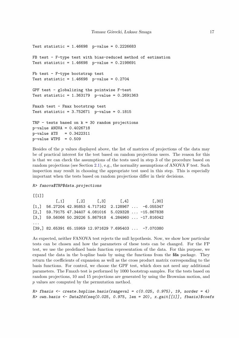
Besides of the p values displayed above, the list of matrices of projections of the data maybe of practical interest for the test based on random projections users. The reason for thisis that we can check the assumptions of the tests used in step 3 of the procedure based onrandom projections (see Section 2.1), e.g., the normality assumptions of ANOVA F test. Suchinspection may result in choosing the appropriate test used in this step. This is especiallyimportant when the tests based on random projections differ in their decisions.

R> fanova$TRP$data.projections

[[1]]

[,1] [,2] [,3] [,4] [,30]

[1,] 56.27204 42.95853 4.717162 2.128967 ... -6.055347

[2,] 59.79175 47.34407 4.081016 5.029328 ... -15.867838

[3,] 59.56066 50.29226 5.867918 4.284960 ... -17.816042

...

[39,] 82.65391 65.15959 12.971629 7.695403 ... -7.070380

As expected, neither FANOVA test rejects the null hypothesis. Now, we show how particulartests can be chosen and how the parameters of these tests can be changed. For the FPtest, we use the predefined basis function representation of the data. For this purpose, weexpand the data in the b-spline basis by using the functions from the fda package. Theyreturn the coefficients of expansion as well as the cross product matrix corresponding to thebasis functions. For control, we choose the GPF test, which does not need any additionalparameters. The Fmaxb test is performed by 1000 bootstrap samples. For the tests based onrandom projections, 10 and 15 projections are generated by using the Brownian motion, andp values are computed by the permutation method.

R> fbasis <- create.bspline.basis(rangeval = c(0.025, 0.975), 19, norder = 4)

R> own.basis <- Data2fd(seq(0.025, 0.975, len = 20), x.gait[[1]], fbasis)$coefs


R> own.cross.prod.mat <- inprod(fbasis, fbasis)

R> set.seed(123)

R> fanova.tests(x.gait[[1]], group.label.gait,

+ test = c("FP", "GPF", "Fmaxb", "TRP"),

+ params = list(paramFP = list(B.FP = 1000, basis = "own",

+ own.basis = own.basis,

+ own.cross.prod.mat =

+ own.cross.prod.mat),

+ paramFmaxb = 1000,

+ paramTRP = list(k = c(10, 15),

+ projection = "BM",

+ permutation = TRUE,

+ B.TRP = 1000)))

Analysis of Variance for Functional Data

FP test - permutation test based on a basis function representation


GPF test - globalizing the pointwise F-test


Fmaxb test - Fmax bootstrap test




p-value ATS = 0.3871429




p-value ATS = 0.507


The above examples concern only the first functional feature of the gait data set. Similaranalysis can be performed for the second one. However, both features can be simultane-ously investigated by using the FMANOVA tests desribed in Section 2.2. First, we considerthe permutation tests based on a basis function representation implemented in the functionfmanova.ptbfr(). We apply this function to the whole data set specifying non-default valuesof most of parameters. Here, we also show how use the function summary.fmanovaptbfr()

to additionally obtain a summary of the data and test parameters. Observe that the resultsare consistent with these obtained by FANOVA tests.

R> set.seed(123)

R> fmanova <- fmanova.ptbfr(x.gait, group.label.gait, int = c(0.025, 0.975),

+ B = 5000, basis = "b-spline", criterion = "eBIC",


+ commonK = "mean", minK = 5, maxK = 20, norder = 4,

+ gamma.eBIC = 0.7)

R> summary(fmanova)

FMANOVA - Permutation Tests based on a Basis Function Representation

Data summary

Number of observations = 39

Number of features = 2

Number of time points = 20

Number of groups = 3

Group labels: 1 2 3

Group sizes: 13 13 13

Range of data = [0.025 , 0.975]

Testing results

W = 0.9077424 p-value = 0.5322

LH = 0.1003732 p-value = 0.5286

P = 0.09340229 p-value = 0.5366

R = 0.08565056 p-value = 0.3852

Parameters of test

Number of permutations = 5000

Basis: b-spline (norder = 4)

Criterion: eBIC (gamma.eBIC = 0.7)

CommonK: mean

Km = 20 20 KM = 20 minK = 5 maxK = 20

Finally, we apply the tests based on random projections for the FMANOVA problem in thegait data set. In the following, these tests are performed with k = 1, 5, 10, 15, 20 projections,standard and permutation methods as well as the random projections generated in indepen-dent and dependent ways. The resulting p values are visualized by the plot.fmanovatrp()

function:

R> set.seed(123)

R> fmanova1 <- fmanova.trp(x.gait, group.label.gait, k = c(1, 5, 10, 15, 20))

R> fmanova2 <- fmanova.trp(x.gait, group.label.gait, k = c(1, 5, 10, 15, 20),

+ permutation = TRUE)

R> plot(x = fmanova1, y = fmanova2)

R> plot(x = fmanova1, y = fmanova2, withoutRoy = TRUE)

R> set.seed(123)


+ independent.projection.tests = FALSE)



0.2

0.4

0.6

0.8

5 10 15 20

k

p−

valu

e

test

LHp

LHpp

Pp

Ppp

Rpp

Wp

Wpp

FMANOVA − Tests based on k Random Projections

0.2

0.4

0.6

0.8

5 10 15 20

k

p−

valu

e

test

LHp

LHpp

Pp

Ppp

Rp

Rpp

Wp

Wpp


0.2

0.4

0.6

0.8

5 10 15 20

k

p−

valu

e

test

LHp

LHpp

Pp

Ppp

Rpp

Wp

Wpp


0.2

0.4

0.6

0.8

5 10 15 20

k

p−

valu

e

test

LHp

LHpp

Pp

Ppp

Rp

Rpp

Wp

Wpp


0.2

0.4

0.6

0.8

5 10 15 20

k

p−

valu

e

test

LHp

LHpp

Pp

Ppp

Rpp

Wp

Wpp


Figure 2: P values of the tests based on random projections for the FMANOVA problem inthe gait data set. The Wpp, LHpp, Ppp and Rpp tests are the permutation versions of theWp, LHp, Pp and Rp tests. In the first (resp. second) row, the random projections weregenerated in independent (resp. dependent) way.

+ permutation = TRUE,

+ independent.projection.tests = FALSE)

R> plot(x = fmanova3, y = fmanova4)

R> plot(x = fmanova3, y = fmanova4, withoutRoy = TRUE)

The obtained plots are shown in Figure 2. As we can observe, except the standard Rp test,all testing procedures behave similarly and do not reject the null hypothesis. The standardRp test does not keep the pre-assigned type-I error rate as Gorecki and Smaga (2017a) shownin simulations. More precisely, this test is usually too liberal, which explains that its p valuesare much smaller than these of the other testing procedures. That is why the function hasoption not to plot the p values of this test.


References

Anderson TW (2003). An Introduction to Multivariate Statistical Analysis. 3rd edition. JohnWiley & Sons, London.

Benjamini Y, Hochberg Y (1995). “Controlling the False Discovery Rate: A Practical andPowerful Approach to Multiple Testing.” Journal of the Royal Statistical Society B, 57,289–300.

Benjamini Y, Yekutieli D (2001). “The Control of the False Discovery Rate in Multiple Testingunder Dependency.” The Annals of Statistics, 29, 1165–1188.

Berrendero JR, Justel A, Svarc M (2011). “Principal Components for Multivariate FunctionalData.” Computational Statistics & Data Analysis, 55, 2619–2634.

Bobelyn E, Serban AS, Nicu M, Lammertyn J, Nicolai BM, Saeys W (2010). “PostharvestQuality of Apple Predicted by NIR-spectroscopy: Study of the Effect of Biological Variabil-ity on Spectra and Model Performance.” Postharvest Biology and Technology, 55, 133–143.

Boente G, Barrera MS, Tyler DE (2014). “A Characterization of Elliptical Distributions andSome Optimality Properties of Principal Components for Functional Data.” Journal of

Multivariate Analysis, 131, 254–264.

Brockhaus S, Rugamer D (2016). FDboost: Boosting Functional Regression Models. R pack-age version 0.2-0, URL https://CRAN.R-project.org/package=FDboost.

Brockhaus S, Scheipl F, Hothorn T, Greven S (2015). “The Functional Linear Array Model.”Statistical Modelling, 15, 279–300.

Brunner E, Dette H, Munk A (1997). “Box-Type Approximations in Nonparametric FactorialDesigns.” Journal of the American Statistical Association, 92, 1494–1502.

Cao G, Yang L, Todem D (2012). “Simultaneous Inference for the Mean Function Based onDense Functional Data.” Journal of Nonparametric Statistics, 24, 359–377.

Chang C, Chen Y, Ogden RT (2014). “Functional Data Classification: A Wavelet Approach.”Computational Statistics, 29, 1497–1513.

Chen D, Hall P, Muller HG (2011). “Single and Multiple Index Functional Regression Modelswith Nonparametric Link.” The Annals of Statistics, 39, 1720–1747.

Chen Y, Keogh E, Hu B, Begum N, Bagnall A, Mueen A, Batista G (2015). “The UCR TimeSeries Classification Archive.” URL http://www.cs.ucr.edu/~eamonn/time_series_

data/.

Cheng Y, Shi JQ (2016). flars: Functional LARS. R package version 1.0, URL https:

//CRAN.R-project.org/package=flars.

Chiou JM, Chen YT, Yang YF (2014). “Multivariate Functional Principal Component Anal-ysis: A Normalization Approach.” Statistica Sinica, 24, 1571–1596.

https://CRAN.R-project.org/package=FDboost

http://www.cs.ucr.edu/~eamonn/time_series_data/

http://www.cs.ucr.edu/~eamonn/time_series_data/

https://CRAN.R-project.org/package=flars

https://CRAN.R-project.org/package=flars


Chiou JM, Muller HG (2014). “Linear Manifold Modelling of Multivariate Functional Data.”Journal of the Royal Statistical Society B, 76, 605–626.

Chiou JM, Yang YF, Chen YT (2016). “Multivariate Functional Linear Regression and Pre-diction.” Journal of Multivariate Analysis, 146, 301–312.

Coffey N, Hinde J, Holian E (2014). “Clustering Longitudinal Profiles Using P-Splines andMixed Effects Models Applied to Time-Course Gene Expression Data.” Computational

Statistics & Data Analysis, 71, 14–29.

Cuesta-Albertos JA, Febrero-Bande M (2010). “A Simple Multiway ANOVA for FunctionalData.” Test, 19, 537–557.

Cuevas A (2014). “A Partial Overview of the Theory of Statistics with Functional Data.”Journal of Statistical Planning and Inference, 147, 1–23.

Cuevas A, Febrero M, Fraiman R (2004). “An Anova Test for Functional Data.”Computational


Dai X, Hadjipantelis PZ, Ji H, Muller HG, Wang JL (2016). fdapace: Functional Data Anal-

ysis and Empirical Dynamics. R package version 0.2.5, URL https://CRAN.R-project.

org/package=fdapace.

Degras DA (2011). “Simultaneous Confidence Bands for Nonparametric Regression withFunctional Data.” Statistica Sinica, 21, 1735–1765.

Delaigle A, Hall P (2012). “Achieving Near Perfect Classification for Functional Data.”Journalof the Royal Statistical Society B, 74, 267–286.

Delaigle A, Hall P (2013). “Classification Using Censored Functional Data.” Journal of the

American Statistical Association, 108, 1269–1283.

Dziak J, Shiyko M (2016). funreg: Functional Regression for Irregularly Timed Data. R pack-age version 1.2, URL https://CRAN.R-project.org/package=funreg.

Faraway J (1997). “Regression Analysis for a Functional Response.” Technometrics, 39,254–261.

Febrero-Bande M, Galeano P, Gonzalez-Manteiga W (2008). “Outlier Detection in FunctionalData by Depth Measures, with Application to Identify Abnormal NOx Levels.” Environ-

metrics, 19, 331–345.

Febrero-Bande M, Oviedo de la Fuente M (2012). “Statistical Computing in Functional DataAnalysis: The R Package fda.usc.” Journal of Statistical Software, 51, 1–28.

Ferraty F, Vieu P (2006). Nonparametric Functional Data Analysis: Theory and Practice.New York.

Fremdt S, Horvath L, Kokoszka P, Steinebach JG (2014). “Functional Data Analysis withIncreasing Number of Projections.” Journal of Multivariate Analysis, 124, 313–332.

Giacofci M, Lambert-Lacroix S, Marot G, Picard F (2013). “Wavelet-Based Clustering forMixed-Effects Functional Models in High Dimension.” Biometrics, 69, 31–40.

https://CRAN.R-project.org/package=fdapace

https://CRAN.R-project.org/package=fdapace

https://CRAN.R-project.org/package=funreg


Goldsmith J, Scheipl F, Huang L, Wrobel J, Gellar J, Harezlak J, McLean MW, SwihartB, Xiao L, Crainiceanu C, Reiss PT (2016). refund: Regression with Functional Data.R package version 0.1-16, URL https://CRAN.R-project.org/package=refund.

Gorecki T, Krzysko M, Waszak L, Wo lynski W (2016a). “Selected Statistical Methods ofData Analysis for Multivariate Functional Data.” Statistical Papers doi:10.1007/s00362-016-0757-8.

Gorecki T, Krzysko M, Wo lynski W (2015). “Classification Problem Based on RegressionModels for Multidimensional Functional Data.” Statistics in Transition New Series, 16,97–110.

Gorecki T, Krzysko M, Wo lynski W (2016b). “Multivariate Functional Regression Analysiswith Application to Classification Problems.” In Studies in Classification, Data Analysis,

and Knowledge Organization: Analysis of Large and Complex Data, pp. 173–183.

Gorecki T, Smaga L (2015). “A Comparison of Tests for the One-Way ANOVA Problem forFunctional Data.” Computational Statistics, 30, 987–1010.

Gorecki T, Smaga L (2017a). “Multivariate Analysis of Variance for Functional Data.” Journalof Applied Statistics, 44, 2172–2189.

Gorecki T, Smaga L (2017b). mfds: Multivariate Functional Data Sets. R package ver-sion 0.1.0, URL https://github.com/Halmaris/mfds.

Hankin RKS (2005). “Recreational Mathematics with R: Introducing the ’magic’ Package.”R News, 5.

Happ C (2017). MFPCA: Multivariate Functional Principal Component Analysis for Data

Observed on Different Dimensional Domains. R package version 1.1, URL https://CRAN.

R-project.org/package=MFPCA.

Happ C, Greven S (2016). “Multivariate Functional Principal Component Analysis for DataObserved on Different (Dimensional) Domains.” Journal of the American Statistical Asso-

ciation. To appear.

Helwig NE (2016). bigsplines: Smoothing Splines for Large Samples. R package version 1.0-9,URL http://CRAN.R-project.org/package=bigsplines.

Hilgert N, Mas A, Verzelen N (2013). “Minimax Adaptive Tests for the Functional LinearModel.” The Annals of Statistics, 41, 838–869.

Hojsgaard S, Halekoh U (2016). doBy: Groupwise Statistics, LSmeans, Linear Contrasts,

Utilities. R package version 4.5-15, URL https://CRAN.R-project.org/package=doBy.

Hormann S, Kidzinski L (2015). freqdom: Frequency Domain Analysis for Multivariate Time

Series. R package version 1.0.4, URL https://CRAN.R-project.org/package=freqdom.

Horvath L, Kokoszka P (2012). Inference for Functional Data with Applications. Springer-Verlag, New York.

Hyndman RJ, Shang HL (2016). ftsa: Functional Time Series Analysis. R package version 4.7,URL http://cran.r-project.org/package=ftsa.

https://CRAN.R-project.org/package=refund

https://github.com/Halmaris/mfds

https://CRAN.R-project.org/package=MFPCA

https://CRAN.R-project.org/package=MFPCA

http://CRAN.R-project.org/package=bigsplines

https://CRAN.R-project.org/package=doBy

https://CRAN.R-project.org/package=freqdom

http://cran.r-project.org/package=ftsa


Jacques J, Preda C (2014). “Model-Based Clustering for Multivariate Functional Data.”Computational Statistics & Data Analysis, 71, 92–106.

James GM, Hastie TJ (2001). “Functional Linear Discriminant Analysis for Irregularly Sam-pled Curves.” Journal of the Royal Statistical Society B, 63, 533–550.

Jank W, Shmueli G (2006). “Functional Data Analysis in Electronic Commerce Research.”Statistical Science, 21, 155–166.

Keser IK, Kocakoc ID (2015). “Smoothed Functional Canonical Correlation Analysis of Hu-midity and Temperature Data.” Journal of Applied Statistics, 42, 2126–2140.

Kidzinski L, Jouzdani N, Kokoszka P (2016). pcdpca: Dynamic Principal Components for

Periodically Correlated Functional Time Series. R package version 0.2.1, URL https:

//CRAN.R-project.org/package=pcdpca.

Krzysko M, Smaga L (2017). “An Application of Functional Multivariate Regression Modelto Multiclass Classification.” Statistics in Transition new series. To appear.

Krzysko M, Waszak L (2013). “Canonical Correlation Analysis for Functional Data.” Biomet-

rical Letters, 50, 95–105.

Leeb R, Lee F, Keinrath C, Scherer R, Bischof H, Pfurtscheller G (2007). “Brain-ComputerCommunication: Motivation, Aim, and Impact of Exploring a Virtual Apartment.” IEEE

Transactions on Neural Systems & Rehabilitation Engineering, 15, 473–482.

Lichman M (2013). “UCI Machine Learning Repository.” URL http://archive.ics.uci.

edu/ml.

Lila E, Sangalli LM, Ramsay J, Formaggia L (2016). fdaPDE: Functional Data Analysis

and Partial Differential Equations; Statistical Analysis of Functional and Spatial Data,

Based on Regression with Partial Differential Regularizations. R package version 0.1-4,URL https://CRAN.R-project.org/package=fdaPDE.

Long W, Li N, Wang H, Cheng S (2012). “Impact of US Financial Crisis on Different Countries:Based on the Method of Functional Analysis of Variance.” Procedia Computer Science, 9,1292–1298.

Ma S, Yang L, Carroll RJ (2012). “A Simultaneous Confidence Band for Sparse LongitudinalRegression.” Statistica Sinica, 22, 95–122.

Maierhofer T (2017). classiFunc: Classification of Functional Data. R package version 0.1.0,URL https://CRAN.R-project.org/package=classiFunc.

Markussen B (2014). fdaMixed: Functional Data Analysis in a Mixed Model Framework.R package version 0.4, URL https://CRAN.R-project.org/package=fdaMixed.

Martınez-Camblor P, Corral N (2011). “Repeated Measures Analysis for Functional Data.”Computational Statistics & Data Analysis, 55, 3244–3256.

Morris JS (2015). “Functional Regression.” Annual Review of Statistics and Its Application,2, 321–359.

https://CRAN.R-project.org/package=pcdpca

https://CRAN.R-project.org/package=pcdpca

http://archive.ics.uci.edu/ml

http://archive.ics.uci.edu/ml

https://CRAN.R-project.org/package=fdaPDE

https://CRAN.R-project.org/package=classiFunc

https://CRAN.R-project.org/package=fdaMixed


Ogden RT, Miller CE, Takezawa K, Ninomiya S (2002). “Functional Regression in CropLodging Assessment with Digital Images.” Journal of Agricultural, Biological, and Envi-

ronmental Statistics, 7, 389–402.

Ojeda Cabrera JL (2012). locpol - Kernel Local Polynomial Regression. R package version 0.6-0, URL http://CRAN.R-project.org/package=locpol.

Olszewski RT (2001). “Generalized Feature Extraction for Structural Pattern Recognition inTime-Series Data.” Ph.D. dissertation, Carnegie Mellon University, Pittsburgh.

Park J, Ahn J (2016). “Clustering Multivariate Functional Data with Phase Variation.”Biometrics doi:10.1111/biom.12546.

Parodi A, Patriarca M, Sangalli L, Secchi P, Vantini S, Vitelli V (2015). fdakma: Func-

tional Data Analysis: K-Mean Alignment. R package version 1.2.1, URL https://CRAN.

R-project.org/package=fdakma.

Pauly M, Brunner E, Konietschke F (2015). “Asymptotic Permutation Tests in GeneralFactorial Designs.” Journal of the Royal Statistical Society B, 77, 461–473.

Peng J, Paul D (2011). fpca: Restricted MLE for Functional Principal Components Analysis.R package version 0.2-1, URL https://CRAN.R-project.org/package=fpca.

Peng QY, Zhou JJ, Tang NS (2016). “Varying Coefficient Partially Functional Linear Regres-sion Models.” Statistical Papers, 57, 827–841.

Pfeiffer RM, Bura E, Smith A, Rutter JL (2002). “Two Approaches to Mutation DetectionBased on Functional Data.” Statistics in Medicine, 21, 3447–3464.

Pini A, Vantini S (2015). fdatest: Interval Testing Procedure for Functional Data. R packageversion 2.1, URL https://CRAN.R-project.org/package=fdatest.

R Core Team (2017). R: A Language and Environment for Statistical Computing. R Founda-tion for Statistical Computing, Vienna, Austria. URL https://www.R-project.org/.

Ramsay JO, Hooker G, Graves S (2009). Functional Data Analysis with R and MATLAB.Springer-Verlag, Berlin.

Ramsay JO, Silverman BW (2005). Functional Data Analysis. 2nd edition. Springer-Verlag,New York.

Ramsay JO, Wickham H, Graves S, Hooker G (2014). fda - Functional Data Analysis.R package version 2.4.4, URL http://CRAN.R-project.org/package=fda.

Revolution Analytics, Weston S (2015). doParallel - Foreach Parallel Adaptor for the ’par-

allel’ Package. R package version 1.0.10, URL http://CRAN.R-project.org/package=

doParallel.

Robbiano S, Saumard M, Cure M (2015). “Improving Prediction Performance of StellarParameters Using Functional Models.” Journal of Applied Statistics, 43, 1465–1476.

Rodriguez JJ, Alonso CJ, Maestro JA (2005). “Support Vector Machines of IntervalbasedFeatures for Time Series Classification.” Knowledge-Based Systems, 18, 171–178.

http://CRAN.R-project.org/package=locpol

https://CRAN.R-project.org/package=fdakma

https://CRAN.R-project.org/package=fdakma

https://CRAN.R-project.org/package=fpca

https://CRAN.R-project.org/package=fdatest

https://www.R-project.org/

http://CRAN.R-project.org/package=fda

http://CRAN.R-project.org/package=doParallel

http://CRAN.R-project.org/package=doParallel


Rossi N, Wang X, Ramsay JO (2002). “Nonparametric Item Response Function Estimateswith the EM Algorithm.” Journal of Educational and Behavioral Statistics, 27, 291–317.

Shang HL (2013). “ftsa: An R Package for Analyzing Functional Time Series.” The R Journal,5, 64–72.

Shang HL, Hyndman RJ (2013). fds: Functional Data Sets. R package version 1.7, URLhttps://CRAN.R-project.org/package=fds.

Shang HL, Hyndman RJ (2016). rainbow: Rainbow Plots, Bagplots and Boxplots for

Functional Data. R package version 3.4, URL https://CRAN.R-project.org/package=

rainbow.

Shen Q, Faraway J (2004). “An F Test for Linear Models with Functional Responses.” Sta-

tistica Sinica, 14, 1239–1257.

Shi JQ, Cheng Y (2014). GPFDA: Apply Gaussian Process in Functional Data Analysis.R package version 2.2, URL https://CRAN.R-project.org/package=GPFDA.

Smaga L (2017). “Repeated Measures Analysis for Functional Data Using Box-Type Approx-imation - with Applications.” REVSTAT. To appear.

S original by Jim Ramsey R port by Brian Ripley (2015). pspline - Penalized Smoothing

Splines. R package version 1.0-17, URL http://CRAN.R-project.org/package=pspline.

Soueidatt M, * (2014). Funclustering: A Package for Functional Data Clustering. R packageversion 1.0.1, URL https://CRAN.R-project.org/package=Funclustering.

Tarabelloni N, Arribas-Gil A, Ieva F, Paganoni AM, Romo J (2017). roahd: Robust Analysisof High Dimensional Data. R package version 1.3, URL https://CRAN.R-project.org/

package=roahd.

Tarrıo-Saavedra J, Naya S, Francisco-Fernandez M, Artiaga R, Lopez-Beceiro J (2011). “Ap-plication of Functional ANOVA to the Study of Thermal Stability of Micro-Nano SilicaEpoxy Composites.” Chemometrics and Intelligent Laboratory Systems, 105, 114–124.

Tavakoli S (2015). ftsspec: Spectral Density Estimation and Comparison for Functional Time

Series. R package version 1.0.0, URL https://CRAN.R-project.org/package=ftsspec.

Tokushige S, Yadohisa H, Inada K (2007). “Crisp and Fuzzy k-Means Clustering Algorithmsfor Multivariate Functional Data.” Computational Statistics, 22, 1–16.

Tucker JD (2017). fdasrvf: Elastic Functional Data Analysis. R package version 1.8.1, URLhttps://CRAN.R-project.org/package=fdasrvf.

Venables WN, Ripley BD (2002). Modern Applied Statistics with S. 4th edition. Springer-Verlag, New York. ISBN 0-387-95457-0, URL http://www.stats.ox.ac.uk/pub/MASS4.

Walter W, Sanchez-Cabo F, Ricote M (2015). “GOplot: An R Package for Visually CombiningExpression Data with Functional Analysis.” Bioinformatics.

Wang JL, Chiou JM, Muller HG (2016). “Functional Data Analysis.” Annual Review of

Statistics and Its Application, 3, 257–292.

https://CRAN.R-project.org/package=fds

https://CRAN.R-project.org/package=rainbow

https://CRAN.R-project.org/package=rainbow

https://CRAN.R-project.org/package=GPFDA

http://CRAN.R-project.org/package=pspline

https://CRAN.R-project.org/package=Funclustering

https://CRAN.R-project.org/package=roahd

https://CRAN.R-project.org/package=roahd

https://CRAN.R-project.org/package=ftsspec

https://CRAN.R-project.org/package=fdasrvf

http://www.stats.ox.ac.uk/pub/MASS4


Wickham H (2009). ggplot2 - Elegant Graphics for Data Analysis. Springer-Verlag, NewYork.

Wrobel J, Goldsmith J (2016). refund.shiny: Interactive Plotting for Functional Data

Analyses. R package version 0.3.0, URL https://CRAN.R-project.org/package=refund.

shiny.

Yamamoto M, Terada Y (2014). “Functional Factorial K-means Analysis.” Computational


Yassouridis C (2016). funcy: Functional Clustering Algorithms. R package version 0.8.5,URL https://CRAN.R-project.org/package=funcy.

Zhang JT (2011). “Statistical Inferences for Linear Models with Functional Responses.” Sta-

tistica Sinica, 21, 1431–1451.

Zhang JT (2013). Analysis of Variance for Functional Data. Chapman & Hall, London.

Zhang JT, Chen JW (2007). “Statistical Inferences for Functional Data.” The Annals of

Statistics, 35, 1052–1079.

Zhang JT, Cheng MY, Tseng CJ, Wu HT (2013). “A New Test for One-Way ANOVA withFunctional Data and Application to Ischemic Heart Screening.” ArXiv:1309.7376v1.

Zhang JT, Liang X (2014). “One-Way ANOVA for Functional Data via Globalizing thePointwise F -Test.” Scandinavian Journal of Statistics, 41, 51–71.

Affiliation:

Tomasz Gorecki, Lukasz SmagaFaculty of Mathematics and Computer ScienceAdam Mickiewicz UniversityUmultowska 87, 61-614 Poznan, PolandE-mail: [email protected], [email protected]

https://CRAN.R-project.org/package=refund.shiny

https://CRAN.R-project.org/package=refund.shiny

https://CRAN.R-project.org/package=funcy

mailto:[email protected], [email protected]

fdanova: an r software package for analysis of variance

Documents