General rights Copyright and moral rights for the publications made accessible in the public portal are retained by the authors and/or other copyright owners and it is a condition of accessing publications that users recognise and abide by the legal requirements associated with these rights.

Users may download and print one copy of any publication from the public portal for the purpose of private study or research.

You may not further distribute the material or use it for any profit-making activity or commercial gain

You may freely distribute the URL identifying the publication in the public portal If you believe that this document breaches copyright please contact us providing details, and we will remove access to the work immediately and investigate your claim.

Downloaded from orbit.dtu.dk on: May 21, 2020

Feature selection for portfolio optimization

Bjerring, Thomas Trier; Ross, Omri; Weissensteiner, Alex

Published in:Annals of Operations Research

Link to article, DOI:10.1007/s10479-016-2155-y

Publication date:2017

Document VersionPeer reviewed version

Link back to DTU Orbit

Citation (APA):Bjerring, T. T., Ross, O., & Weissensteiner, A. (2017). Feature selection for portfolio optimization. Annals ofOperations Research, 256(1), 21-40. https://doi.org/10.1007/s10479-016-2155-y

Feature Selection for Portfolio Optimization

Thomas Trier BjerringTechnical University of Denmark

Omri RossTechnical University of Denmark and

University of Copenhagen

Alex WeissensteinerTechnical University of Denmark andFree University of Bozen-Bolzano

January 26, 2016

Abstract

Most portfolio selection rules based on the sample mean and covariance matrix

perform poorly out-of-sample. Moreover, there is a growing body of evidence that

such optimization rules are not able to beat simple rules of thumb, such as 1/N.

Parameter uncertainty has been identified as one major reason for these findings. A

strand of literature addresses this problem by improving the parameter estimation

and/or by relying on more robust portfolio selection methods. Independent of the

chosen portfolio selection rule, we propose using feature selection first in order to

reduce the asset menu. While most of the diversification benefits are preserved, the

parameter estimation problem is alleviated. We conduct out-of-sample back-tests to

show that in most cases different well-established portfolio selection rules applied on

the reduced asset universe are able to improve alpha relative to different prominent

factor models.

Keywords: Portfolio Optimization, Parameter Uncertainty, Feature Selection,

Agglomerative Hierarchical Clustering

1 Introduction

The seminal work of Markowitz (1952) has inspired a lot of work in the field of asset

allocation. However, the solutions obtained by such techniques are usually very sensi-

tive to the input parameters (see e.g. Best and Grauer, 1991) with the consequence that

estimation errors lead to unstable and extreme positions in single assets. Chopra and

Ziemba (1993) are one of the first to quantify the consequences of misspecified parame-

ters in asset allocation decisions. Specifically, they illustrate that in their setting errors

1

in expected returns are about ten times more important than errors in variances and

covariances. Furthermore, in addition to the general consensus that expected returns

are notoriously difficult to predict, Merton (1980) shows that even if the true parameters

were constant, very long time series would be required to estimate expected returns in

a reliable way. As a consequence, a trading strategy based on the sample minimum

variance portfolio, which completely abstains from estimating expected returns, shows

a better risk-adjusted performance than many other portfolio selection rules (see e.g.

Haugen and Baker, 1991; Clarke et al., 2006; Scherer, 2011). Others propose different

techniques to alleviate the problem of estimating expected returns. Jorion (1986) con-

siders explicitly the potential utility loss when using sample means to estimate expected

returns. In order to minimize this loss function, he uses Bayes-Stein estimation to shrink

the sample means toward a common value. A simulation study shows that this correc-

tion provides significant gains. Black and Litterman (1992) argue that the only sensible

“neutral” expected returns are those that would clear the market if all investors had

identical views. Hence, the natural choice are the equilibrium expected returns derived

from reverse optimization using the current market capitalization. Having these “neu-

tral expected returns” as a starting point, they illustrate how to combine them with an

investor’s own view in a statistically consistent way.

Kan and Zhou (2007) show that there is a very significant interactive effect between

the estimation of the parameters and the ratio of the number of assets to the number of

observations. If the number of assets is small compared to the number of observations,

then the estimation of expected returns is more important (in line with Chopra and

Ziemba, 1993). However, when this fraction grows, then estimation errors in the sample

covariance grow too, and may become more severe in terms of utility costs than the

estimation errors in expected returns. Furthermore, when the number of assets exceeds

the number of observations, the sample covariance matrix is always singular (even if the

true covariance matrix is known to be non-singular). Many papers address the problem

of estimating the covariance matrix from limited sample data.

Ledoit and Wolf (2003, 2004a,b, 2012) propose using the “shrinkage” technique in

order to pull extreme coefficients in the sample covariance matrix, which tend to con-

tain a lot of error, towards more central values of a highly structured estimator. They

derive the optimal shrinkage intensity in terms of a loss function, and they suggest

using factor models1 or constant correlation models as structured estimators. Given

that weight constraints improve the performance of mean-variance efficient portfolios,

Jagannathan and Ma (2003) study the short-sale constrained minimum-variance port-

1See Kritzman (1993) who compares factor analysis and cross-sectional regression for that purpose.

2

folio. They show that the optimal solution under short-sale constraints corresponds to

the optimal solution of the unconstrained problem if shrinkage is used to estimate the

covariance matrix, i.e. there is a one-to-one relationship between short-sale constraints

and the shrinkage technique. DeMiguel et al. (2009a) generalize these results by solving

the classical minimum-variance problem under norm-constrained asset weights. They

show that their setting nests the shrinkage technique of Ledoit and Wolf (2003, 2004a)

and Jagannathan and Ma (2003) as special cases. Given that for more volatile stocks the

parameter estimation risk is higher, Levy and Levy (2014) propose two variance-based

constraints to alleviate the problem of parameter uncertainty. First, the Variance-Based

Constraints on the single weights, which are inversely proportional to the sample stan-

dard deviation of each asset. Second, the Global Variance-Based Constraints, where

instead of sharp boundary constraints on each stock a quadratic “cost” is assigned to

deviations from an equally weighted portfolio. Comparing ten optimization methods,

they find that the two new suggested methods typically yield the best performance in

terms of Sharpe ratio.

Another method to mitigate the estimation problem uses more portfolios than those

proposed by the classical two-funds Tobin separation theorem. Kan and Zhou (2007)

suggest adding a third risky fund to the risk-free asset and to the sample tangency port-

folio to hedge against parameter uncertainty. In particular, under the assumption of

constant parameters, they show that a portfolio which optimally combines the risk-free

asset, the sample tangency portfolio (TP) and the sample global minimum-variance port-

folio (MVP) dominates a portfolio with just the risk-free asset and the sample tangency

portfolio.

The most extreme approach to address the problem of parameter uncertainty is to

ignore all historical observations and to invest equally in the available assets. Such a

strategy is known as the 1/N rule. Duchin and Levy (2009) use the 30 Fama-French

industry portfolios (2001–2007) to compare the 1/N rule against a Markowitz mean-

variance rule under short-sale constraints. They illustrate that for a low number of

assets (below 25) the 1/N rule provides a higher average out-of-sample return. Only if

all 30 assets are traded, then the classical optimization approach outperforms the 1/N

rule slightly. DeMiguel et al. (2009b) compare 14 portfolio selection rules across seven

empirical datasets and show that none is consistently better out-of-sample than the 1/N

rule. Furthermore, under the assumption of constant parameters, they show that time-

series of extreme length (more than 6000 months for 50 assets) are necessary to beat the

1/N benchmark.

Given the results of DeMiguel et al. (2009b), Tu and Zhou (2011) combine the 1/N

3

rule with four other well-known portfolio selection rules. Among others, they extend

the Kan and Zhou (2007) model and propose adding the equally weighted 1/N portfolio

as a fourth fund in an optimal way to reduce the estimation error. The MVP and the

1/N portfolio are natural candidates: While the MVP does not depend on expected

returns, for the 1/N portfolio neither expected returns nor a covariance matrix have to

be estimated.2

The results given by DeMiguel et al. (2009b) raise serious concerns about portfolio

optimization altogether. In defense of optimization, Kritzman et al. (2010) argue that

most studies rely on too short samples for estimating expected returns, which often

yields implausible results. They show that when estimations of expected excess returns

are based on long-term samples, then usually optimized portfolios outperform equally

weighted portfolios.

To sum up: Many of the aforementioned papers illustrate that the problem of pa-

rameter uncertainty increases with the number of assets (see e.g. Kan and Zhou, 2007).

Different data mining techniques such as factor models (see e.g. Kritzman, 1993), shrink-

age of the mean (see e.g. Jorion, 1986) and shrinkage of the covariance (see e.g. Ledoit

and Wolf, 2003, 2004a) are proposed to alleviate the problem of the parameter estima-

tion. Under the assumption of constant parameters, extending the observation period

improves the performance of optimization based portfolio rules (see e.g. DeMiguel et al.,

2009b; Kritzman et al., 2010). However, whether parameters are really constant over

time is questionable, which suggests that simply expanding the observation period might

not be the best strategy in practice.

Compared to the above mentioned literature, in this paper we propose using fea-

ture selection by agglomerative hierarchical clustering. Based on correlation, we create

groups of assets such that the similarity within a cluster and the dissimilarity between

different clusters is maximized. From each group we select then one representative asset

to construct a smaller but yet comprehensive enough universe.3 As the representative

asset we use the medoid, whose average dissimilarity to all the objects in the cluster

is minimal. While the reduced asset menu facilitates the estimation of the parameters,

the chosen assets still allow to benefit from diversification. Our choice is motivated by

previous studies. Tola et al. (2008) show that clustering algorithms can improve the

reliability of the portfolio in terms of the ratio between predicted and realized risk. Lisi

and Corazza (2008) use clustering for a practical portfolio optimization task under car-

2For the rest of the paper, when referring to the Tu and Zhou (2011) strategy, we mean the optimalcombination of 1/N with Kan and Zhou (2007).

3In the following we use the term “feature selection” as synonym for “hierarchical clustering”.

4

dinality constraints. They use different distance functions and illustrate that in general

clustering improves the out-of-sample performance compared to a benchmark. Nanda

et al. (2010) compare different clustering techniques (as K-means, Fuzzy C-means, Self

Organizing Maps) for portfolio management in the Indian market and report benefits

compared to the benchmark (the Sensex index).

The present work makes four contributions to the literature on clustering in port-

folio optimization. First, compared to the above mentioned papers, our out-of-sample

back-tests are based on long and well-known time series. Specifically, we use the value-

weighted 49 industry portfolios provided by Kenneth French4 as well as the constituent

stocks of the S&P 500. For both data sets, we use monthly returns from 1970 to 2013.

Second, in addition to the classical minimum-variance portfolio and the tangency port-

folio, we consider also the more advanced portfolio selection rules suggested by Kan and

Zhou (2007) and Tu and Zhou (2011). We compare pairwise the results with and without

feature selection.5 Furthermore, feature selection allows to use these portfolio selection

rules also on data sets with more assets than observations. Third, in line with Kritzman

et al. (2010) we highlight the importance of the length of the observation period by

presenting back-test results for rolling windows of 5, 10, 15 and 20 years. Finally, we

base our assessment on the alpha relative to the most prominent factor models, such

as Fama and French (1993) and Carhart (1997). As a main result, we show that for

most test cases the performance of the reduced asset universe improves. In particular,

we show that the alpha of the 1/N strategy also benefits from reducing the asset menu.

As the 1/N rule is not prone to parameter estimation errors, this result might be coun-

terintuitive. We explain this finding with other beneficial properties of feature selection.

First, in addition to alleviating the problems due to parameter estimation, the concen-

tration risk of a portfolio is also reduced. To illustrate this point, consider the fact that

over 20% of the stocks in the S&P 500 are from the technology sector. As a result, the

1/N portfolio has high concentration risk in this sector. Feature selection forms groups

such that the intra-group similarity and the inter-group dissimilarity is maximized, i.e.

similar stocks are allocated to the same group. By choosing then a representative asset

out of each group such sector-concentration risks are mitigated. Second, we show that

for appropriate observation periods feature selection reduces the beta of the 1/N portfo-

lio, which relates to the “betting-against-beta” idea proposed by Frazzini and Pedersen

(2014).

4see http://mba.tuck.dartmouth.edu/pages/faculty/ken.french/data_library.html5Given the focus of this paper, we want to point out that the proposed investigation is not intended

as a horse race between the different portfolio selection rules.

5

The paper is structured as follows. Section 2 summarizes the classical portfolio

optimization techniques which are used in this paper. Section 3 offers a more detailed

explanation of how we use feature selection for the problem at hand. Section 4 describes

the data and the results of using feature selection in practice, and Section 5 concludes.

2 Classical Mean-Variance Optimization

Portfolio selection according to Markowitz is based on the assumption of multivariate

normal asset returns. An investor, faced with the decision on how to allocate funds to

N risky and one riskless asset, optimizes the trade-off between the expectation and the

variance of the portfolio returns. This preference can be formulated as

maxw

wᵀµ− λ

2wᵀΣw,

where w = (w1, ..., wi, ..., wN )ᵀ represents the weights allocated to each risky asset in

the portfolio, µ is the vector of expected excess returns over the risk free rate, λ denotes

the risk aversion coefficient, and Σ is the variance-covariance matrix. Consequently, the

difference 1− 1ᵀw is invested in the riskless asset.

In practice the parameters µ and Σ are unknown, i.e. the portfolio optimization has

to be conducted under parameter uncertainty. Estimation errors can have a substantial

influence on the out-of-sample performance of the model, and may lead to solutions

that are far away from the true optimal portfolios (see DeMiguel and Nogales, 2009).

In order to alleviate parameter uncertainty, Kan and Zhou (2007) propose a three-fund

rule, which, in addition to the risk-free asset and the tangent portfolio, engages a third

risky portfolio to hedge against the estimation risk. Furthermore, Tu and Zhou (2011)

extend the three-fund rule and introduce the 1/N portfolio as a fourth portfolio.

DeMiguel et al. (2009b) show with a simulation study that the impact of parameter

uncertainty on the performance of optimized portfolios depends heavily on the number of

included assets. Given constant parameters, they illustrate that very long time series are

needed to estimate µ and Σ precisely enough to outperform an equally weighted portfolio.

In reality, however, parameter values may vary over time, i.e. simply expanding the

estimation window might induce the risk of using outdated observations.

Therefore, instead of simply expanding the window for the parameter estimation, in

this paper we suggest a preliminary screening of the assets considered for optimization

to reduce the dimensionality of the parameter estimation problem, and hereby improve

the out-of-sample quality of the results.

6

In order to assess the performance of feature selection, we compare pairwise the

results of five different portfolio rules with and without reduction of the asset universe.

More specifically, these asset allocation rules are the global minimum variance portfolio,

the tangency mean-variance portfolio, the three-fund portfolio, the four-fund portfolio,

and the 1/N portfolio. A short presentation of them is provided below.

Global Minimum Variance Portfolio

The minimum variance portfolio is a special case in the mean-variance portfolio frame-

work, where the combination of risky assets is chosen such that the total variance of the

portfolio returns is minimized, that is

minw

wᵀΣw

s.t. 1ᵀw = 1.

As this rule relies only on the estimation of the covariance matrix of asset returns, and

ignores the expected returns, it is less prone to estimation errors as fewer parameters

have to be estimated. Analytically, the weights of the minimum variance portfolio can

be expressed as

w∗MV =

Σ−11

1ᵀΣ−11. (1)

Mean-Variance Tangency Portfolio

Tobin (1958) expands Markowitz’ seminal work for a risk-free asset and shows that the

asset allocation task results in maximizing the Sharpe ratio of the portfolio

maxw

wᵀµ√wᵀΣw

s.t. 1ᵀw = 1.

Thereafter, dependent on the investor’s risk aversion, a combination between the result-

ing tangency portfolio and the risk-free asset is chosen. Analytically, the weights of the

tangency portfolio are given by

w∗TP =

Σ−1µ

1ᵀΣ−1µ. (2)

7

The Three-Fund Rule

If the true mean and covariance of asset returns could be estimated precisely, as as-

sumed in theory, then the two-fund separation would hold perfectly. However, when

the parameters are unknown, the tangency portfolio is obtained with estimation errors.

Intuitively, by using an additional risky portfolio the estimation problem can be allevi-

ated. Kan and Zhou (2007) propose using the global minimum-variance portfolio as a

third fund. As the estimation errors of the minimum variance portfolio and the tangency

portfolio are not perfectly correlated, an optimal combination of them allows to improve

the out-of-sample performance. The non-normalized weights of the combined portfolios

are given by

wKZ =c3γ

(cΣ−1µ+ fΣ−11

), (3)

where c and f are chosen optimally to maximize the expected utility of a mean-variance

investor given the relative risk aversion parameter γ and the constant scalar c3 =(T−N−1)(T−N−4)

T (T−2) . The allocation of funds to each of the risky portfolios depends on

the number of assets N and the length of the estimation window T . The more severe

the parameter estimation problem, the higher the optimal proportion invested in the

global minimum variance portfolio. In line with DeMiguel et al. (2009b), we set γ equal

to 1, and we only focus on the composition of the risky part of the suggested portfolios.

More specifically, we calculate the relative weights of the risky assets by

w∗KZ =

wKZ

|1ᵀwKZ |, (4)

where |1ᵀwKZ | guarantees that the direction of the portfolio position is preserved in

cases where the sum of the weights of the risky assets is negative.

The Four-Fund Rule

DeMiguel et al. (2009b) show that the 1/N portfolio rule is difficult to outperform,

especially if the observation period is short. However, as the 1/N rule makes no use

of the sample information, it will fail to converge to the true optimal portfolio (unless,

by chance, the two are the same). Therefore, if 1/N is far from the optimal portfolio

its performance might be poor. Tu and Zhou (2011) propose the four-fund rule by

combining the three fund-rule (see Kan and Zhou, 2007) in an optimal way with the

1/N portfolio. The non-normalized weights of this portfolio combination rule are

wTZ = (1− δ)we + δwKZ , (5)

8

where we is the equally weighted (1/N) portfolio and wKZ is the (non-normalized) opti-

mal portfolio defined by the three-fund rule. The parameter δ, which defines the ratio of

wealth allocated to each of the portfolios, is determined by the number of assets N and

the number of observations T . The larger the number of assets relative to the number

of observations, the more is invested in the 1/N portfolio, and the suggested portfolio

becomes less prone to estimation errors. As in equation (4), we normalize the portfolio

weights as

w∗TZ =

wTZ

|1ᵀwTZ |. (6)

In general, the above mentioned papers assume unknown but constant parameters,

which have to be estimated from historical observations. To mitigate the estimation

problem, an increasing number of assets N requires more observations T . In the limit

– due to the Law of Large Numbers – the estimated parameters converge towards their

true values. However, in case of time-varying investment opportunities and/or structural

breaks, historical data may not correctly reflect the current state of the markets. On the

other hand, for N > T , the sample covariance matrix is always singular. Therefore, it is

natural to investigate whether it is beneficial to reduce the size of the asset menu and

apply the portfolio rules to a representative subset, which reflects the overall dependence

structure. The next section provides a detailed explanation (and a few examples) on

how to reduce the asset universe using feature selection.

3 Dimensionality Reduction Using Feature Selection

This part of the paper proposes a heuristic, namely agglomerative hierarchical clustering,

which exploits the underlying correlation structure of the complete universe in order to

reduce the size of an N -dimensional asset universe significantly. The starting point for

the clustering is the covariance matrix after shrinkage, for which we rely on a constant

correlation matrix (set equal to the sample average) as structured estimator (see Ledoit

and Wolf, 2004b).

3.1 Heterogeneity of the Asset Universe

In order to benefit from diversification when applying portfolio selection rules, the re-

duced subset n ⊂ N should consist of the n assets with the lowest overall correlation

with each other. Identifying this sub-space can be translated into the problem of finding

the longest path of n ⊂ N vertices in a simple cycle of an undirected graph. The distance

between the vertices can be represented by di,j = 1 − ρi,j , where ρi,j is the correlation

9

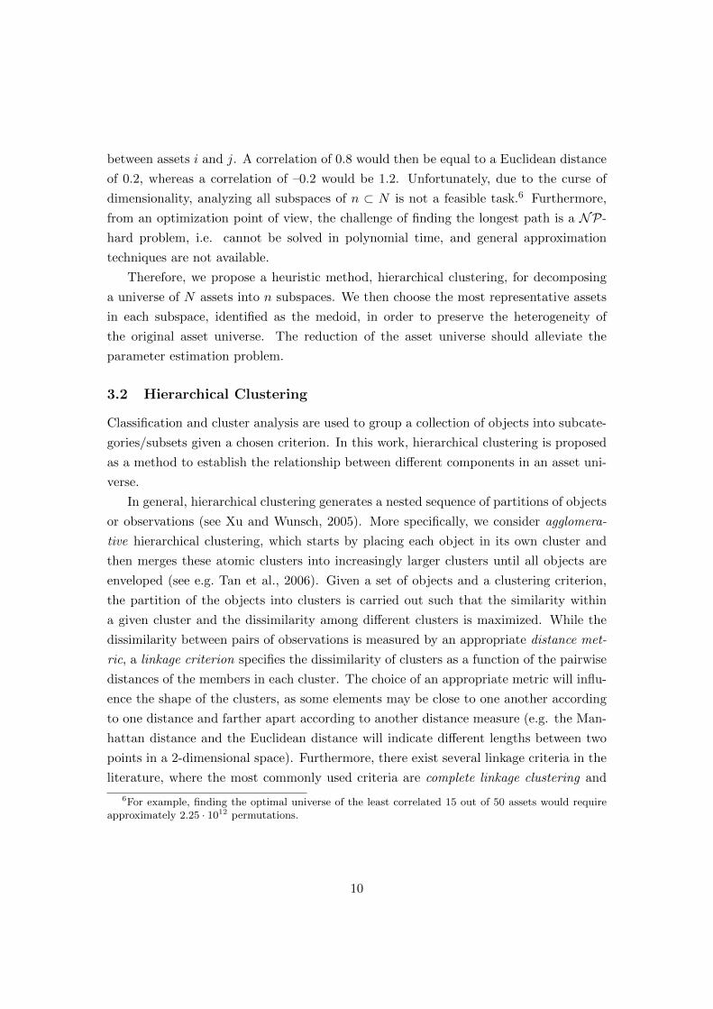
between assets i and j. A correlation of 0.8 would then be equal to a Euclidean distance

of 0.2, whereas a correlation of –0.2 would be 1.2. Unfortunately, due to the curse of

dimensionality, analyzing all subspaces of n ⊂ N is not a feasible task.6 Furthermore,

from an optimization point of view, the challenge of finding the longest path is a NP-

hard problem, i.e. cannot be solved in polynomial time, and general approximation

techniques are not available.

Therefore, we propose a heuristic method, hierarchical clustering, for decomposing

a universe of N assets into n subspaces. We then choose the most representative assets

in each subspace, identified as the medoid, in order to preserve the heterogeneity of

the original asset universe. The reduction of the asset universe should alleviate the

parameter estimation problem.

3.2 Hierarchical Clustering

Classification and cluster analysis are used to group a collection of objects into subcate-

gories/subsets given a chosen criterion. In this work, hierarchical clustering is proposed

as a method to establish the relationship between different components in an asset uni-

verse.

In general, hierarchical clustering generates a nested sequence of partitions of objects

or observations (see Xu and Wunsch, 2005). More specifically, we consider agglomera-

tive hierarchical clustering, which starts by placing each object in its own cluster and

then merges these atomic clusters into increasingly larger clusters until all objects are

enveloped (see e.g. Tan et al., 2006). Given a set of objects and a clustering criterion,

the partition of the objects into clusters is carried out such that the similarity within

a given cluster and the dissimilarity among different clusters is maximized. While the

dissimilarity between pairs of observations is measured by an appropriate distance met-

ric, a linkage criterion specifies the dissimilarity of clusters as a function of the pairwise

distances of the members in each cluster. The choice of an appropriate metric will influ-

ence the shape of the clusters, as some elements may be close to one another according

to one distance and farther apart according to another distance measure (e.g. the Man-

hattan distance and the Euclidean distance will indicate different lengths between two

points in a 2-dimensional space). Furthermore, there exist several linkage criteria in the

literature, where the most commonly used criteria are complete linkage clustering and

6For example, finding the optimal universe of the least correlated 15 out of 50 assets would requireapproximately 2.25 · 1012 permutations.

10

single linkage clustering :

Complete linkage max{d(a, b) : a ∈ A, b ∈ B}

Single linkage min{d(a, b) : a ∈ A, b ∈ B},

where d is a distance measure. While in single-linkage clustering the similarity of two

clusters is given by the similarity of their most similar members, in complete-linkage

clustering the similarity of two clusters is determined by their most dissimilar members.

Hence, using different linkage criteria has a large influence on the size and shape of the

clusters, and choosing an appropriate distance metric and linkage criteria is therefore

crucial when classifying elements in a universe. Single linkage clustering is prone to

the so-called chaining phenomenon, where clusters may be forced together due to single

elements being close to each other, even though many of the elements in each cluster

may be very distant from each other. Complete linkage avoids this drawback and tends

to find compact clusters of approximately equal diameters. Therefore, we adopt the

method of complete linkage in this paper (for a discussion on single- versus complete

linkage see Hartigan, 1981).

As established earlier, correlation is a feasible distance measure. Therefore, agglom-

erative hierarchical clustering can be used to identify and cluster assets into a hierarchical

structure according to their correlation, and a pruning level determines the number of

clusters. Although the distance matrix used in the hierarchical clustering has to be es-

timated, this estimation is only used as a basis for the preliminary coarse grid and not

as a direct input parameter in the portfolio optimization, i.e. the problem of parame-

ter uncertainty is less severe. For all cases we use shrinkage to estimate the covariance

matrix as proposed by Ledoit and Wolf (2004b), with a constant correlation matrix as

structured estimator. In this way, the estimation error is reduced and the requirement

of a non-singular matrix is satisfied.

When the overall structure of the universe is established and n groups (also called

clusters or sets) are formed, representative assets (so-called pillars) are chosen from each

cluster to constitute a reduced asset menu on which the portfolio rules are applied. As

the representative asset we use the medoid.

3.3 Exhibition

In order to illustrate the proposed technique in a still confined data set, we use the

49 industry portfolios from Kenneth French’s website. The 49 industry portfolios are

11

composed of stocks traded on the NYSE, AMEX, and NASDAQ according to their four-

digit SIC code. The monthly data span the period January 1970 to July 2013. First, we

use the shrinkage technique to compute the 49× 49 correlation matrix and transform it

to a Euclidean distance matrix. We then use agglomerative hierarchical clustering with

a complete linkage criterion.

The dendrogram in Figure 1 illustrates at which level the different sub-clusters are

merged. Portfolios which are highly correlated, i.e. have a small distance to their

0.00

0.25

0.50

0.75

Gol

dC

oal

Oil

Sm

oke

Util

Telc

mS

oda

Med

Eq

Dru

gsF

ood

Bee

rH

shld

Hlth

Per

Sv

Shi

psG

uns

Agr

icS

oftw

Har

dwC

hips

LabE

qM

ines

Ste

elM

ach

Cns

trFa

bPr

Box

esTo

ysM

eals

Clth

sR

tail

Aut

osT

xtls

RlE

stF

unB

ooks

Rub

brB

usS

vW

hlsl

Fin

Ban

ksIn

sur

Oth

erA

ero

Bld

Mt

Elc

Eq

Tran

sC

hem

sP

aper

Dis

tanc

e

Dendrogram of the 49 industry portfolios

Figure 1: Dendrogram illustrating the correlation structure of the 49 industry portfolios

neighbors, are linked together at an early stage. One example is the portfolios Mines,

Steel, and Mach. The three portfolios denote the mining, the steel, and the machinery

industries, respectively, which due to their business sectors are highly interconnected.

The tree structure of the dendrogram can be exploited to form groups of assets. By

pruning at specific levels of the tree, a desired number of sets can be constructed. For

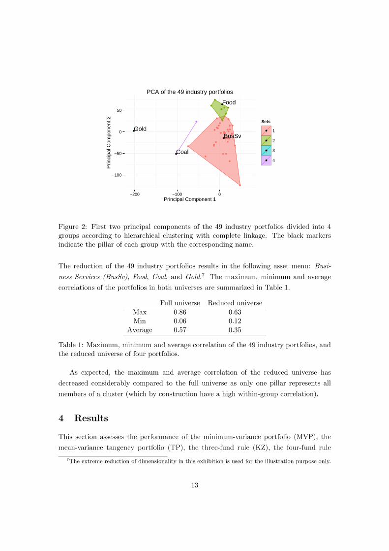
the purely illustrative purpose here, we decide to reduce the universe to n = 4. The

result of maximizing the inter-cluster dissimilarity and the intra-cluster similarity can

be visualized with a principal component analysis (PCA). Figure 2 shows the convex

hull of each cluster projected on the first two principal components. Furthermore, their

corresponding pillars are indicated with a black bullet. It can be seen that the portfolios

are not evenly distributed across the different clusters. Set 1 holds a particularly large

amount of portfolios, while set 3 is a single portfolio. By projecting the 49 dimensions of

this example onto the first two principal components, the areas of sets 1 and 2 overlap.

Of course, in the multidimensional space the convex hulls of the two sets do not overlap.

12

BusSv

Food

Gold

Coal

−100

−50

0

50

−200 −100 0Principal Component 1

Prin

cipa

l Com

pone

nt 2 Sets

1

2

3

4

PCA of the 49 industry portfolios

Figure 2: First two principal components of the 49 industry portfolios divided into 4groups according to hierarchical clustering with complete linkage. The black markersindicate the pillar of each group with the corresponding name.

The reduction of the 49 industry portfolios results in the following asset menu: Busi-

ness Services (BusSv), Food, Coal, and Gold.7 The maximum, minimum and average

correlations of the portfolios in both universes are summarized in Table 1.

Full universe Reduced universe

Max 0.86 0.63Min 0.06 0.12

Average 0.57 0.35

Table 1: Maximum, minimum and average correlation of the 49 industry portfolios, andthe reduced universe of four portfolios.

As expected, the maximum and average correlation of the reduced universe has

decreased considerably compared to the full universe as only one pillar represents all

members of a cluster (which by construction have a high within-group correlation).

4 Results

This section assesses the performance of the minimum-variance portfolio (MVP), the

mean-variance tangency portfolio (TP), the three-fund rule (KZ), the four-fund rule

7The extreme reduction of dimensionality in this exhibition is used for the illustration purpose only.

13

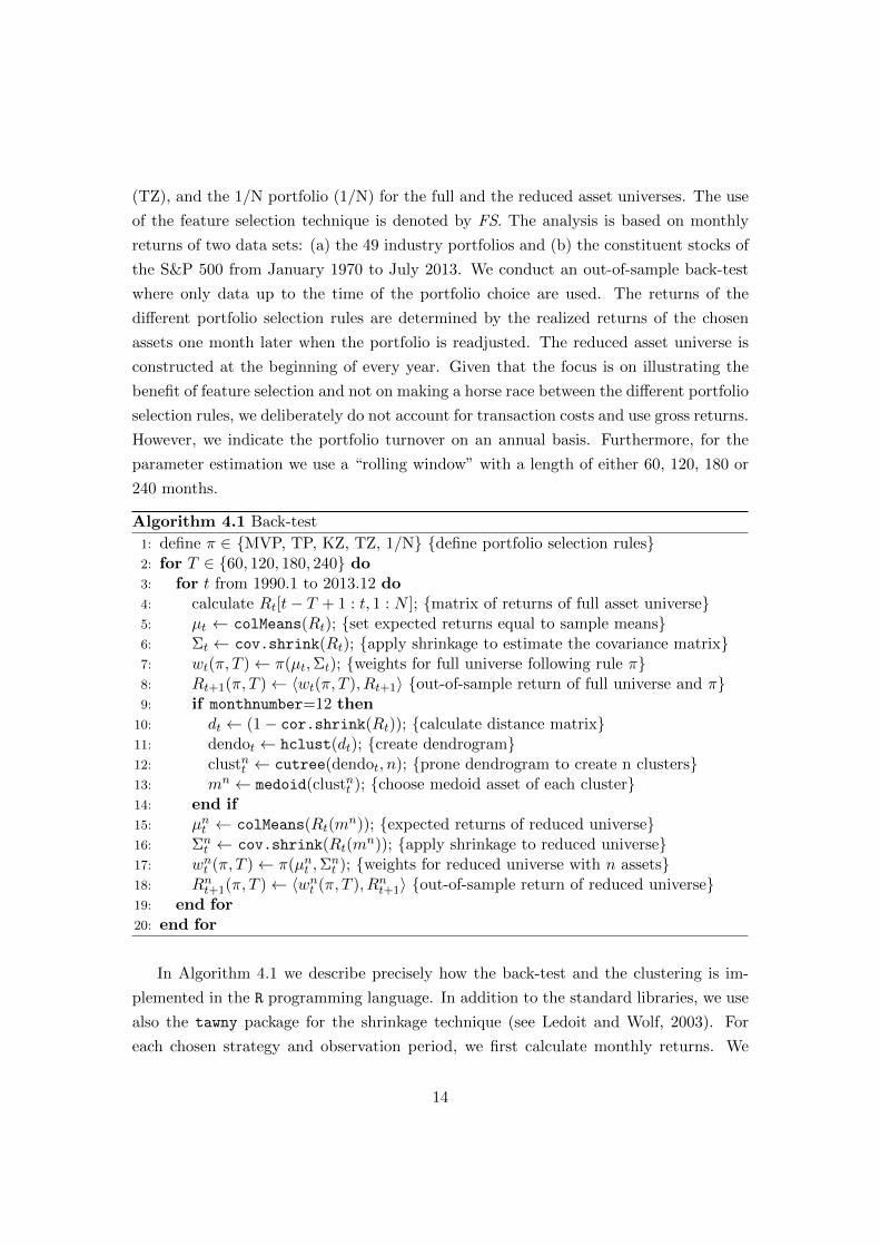
(TZ), and the 1/N portfolio (1/N) for the full and the reduced asset universes. The use

of the feature selection technique is denoted by FS. The analysis is based on monthly

returns of two data sets: (a) the 49 industry portfolios and (b) the constituent stocks of

the S&P 500 from January 1970 to July 2013. We conduct an out-of-sample back-test

where only data up to the time of the portfolio choice are used. The returns of the

different portfolio selection rules are determined by the realized returns of the chosen

assets one month later when the portfolio is readjusted. The reduced asset universe is

constructed at the beginning of every year. Given that the focus is on illustrating the

benefit of feature selection and not on making a horse race between the different portfolio

selection rules, we deliberately do not account for transaction costs and use gross returns.

However, we indicate the portfolio turnover on an annual basis. Furthermore, for the

parameter estimation we use a “rolling window” with a length of either 60, 120, 180 or

240 months.

Algorithm 4.1 Back-test

1: define π ∈ {MVP, TP, KZ, TZ, 1/N} {define portfolio selection rules}2: for T ∈ {60, 120, 180, 240} do3: for t from 1990.1 to 2013.12 do4: calculate Rt[t− T + 1 : t, 1 : N ]; {matrix of returns of full asset universe}5: µt ← colMeans(Rt); {set expected returns equal to sample means}6: Σt ← cov.shrink(Rt); {apply shrinkage to estimate the covariance matrix}7: wt(π, T )← π(µt,Σt); {weights for full universe following rule π}8: Rt+1(π, T )← 〈wt(π, T ), Rt+1〉 {out-of-sample return of full universe and π}9: if monthnumber=12 then

10: dt ← (1− cor.shrink(Rt)); {calculate distance matrix}11: dendot ← hclust(dt); {create dendrogram}12: clustnt ← cutree(dendot, n); {prone dendrogram to create n clusters}13: mn ← medoid(clustnt ); {choose medoid asset of each cluster}14: end if15: µnt ← colMeans(Rt(m

n)); {expected returns of reduced universe}16: Σn

t ← cov.shrink(Rt(mn)); {apply shrinkage to reduced universe}

17: wnt (π, T )← π(µnt ,Σ

nt ); {weights for reduced universe with n assets}

18: Rnt+1(π, T )← 〈wn

t (π, T ), Rnt+1〉 {out-of-sample return of reduced universe}

19: end for20: end for

In Algorithm 4.1 we describe precisely how the back-test and the clustering is im-

plemented in the R programming language. In addition to the standard libraries, we use

also the tawny package for the shrinkage technique (see Ledoit and Wolf, 2003). For

each chosen strategy and observation period, we first calculate monthly returns. We

14

use them to compute the sample means and apply shrinkage to estimate the covariance

matrix on the full asset menu (lines 4–6).8 Then, for optimal portfolios according to

the different selection rules, we calculate an out-of-sample return over the next month

(lines 7–8). The Euclidean scalar product is denoted by 〈·, ·〉. At the end of each year

we choose representative assets for the next year.9 Therefore, in line 10, we calculate

the distance matrix (distance measure is equal to one minus the correlation) that is used

by the clustering algorithm. In lines 11 and 12, we calculate the dendrogram of the full

asset universe and prune the tree to obtain n clusters. Throughout our calculations we

have used exactly 15 clusters for both the 49 industry portfolios and the S&P 500. Then,

we choose the medoid to be the representative asset in each cluster, see line 13. Lines

15–18 repeat the operations 5–8 on the reduced asset menu. Our back-test was run on

a machine with Intel core i5 (2.53 GHz, 3MB L3 cache) and 8 GB RAM. For the S&P

500 data set, all calculations of the back-test can be conducted in less than one hour.10

1970 1971 1972 1973 1974 1975

60 months for parameter estimation

Figure 3: Example for the back-test approach (with an estimation window of 60 months).

Figure 3 shows the back-test approach for a rolling window of 60 months (solid brace)

at the end of year 1974, when parameters are estimated for the first time and when the

portfolio is optimized according to the different portfolio selection rules. One month

later the return of the chosen portfolio is measured and the time window for parameter

estimation is shifted by one month (dashed brace). Given that we use all available data

for all the different observation periods, the number of out-of-sample returns differs.

While, e.g., for an estimation window of 60 months 463 out-of-sample returns can be

calculated, this number reduces to 283 in case of a 240 months window. Furthermore, in

order to avoid that our performance comparisons are determined by a specific inception

date, in addition to the assessment over the whole period we also evaluate realized

returns of the different portfolio rules over consecutive 10 year periods (shifted by one

year). This iterative testing of the portfolio rules is applied until the back-test ends in

8The structured estimator is based on the constant correlation matrix (set equal to the average samplecorrelation), which corresponds to the default value in the package.

9Given that the clusters are quite stable over time and the assets within a cluster are highly correlated,in order to reduce excessive trading we propose to apply feature selection on an annual basis.

10The most time consuming operation is shrinkage. For the 49 industry portfolios the computationaltime for all results is less than 10 minutes.

15

the year 2013. This means that each portfolio rule is evaluated repeatedly on each data

set (with and without feature selection) and with each of the four rolling windows.

The performance assessment of the different portfolio rules is based on annualized

alpha. Alpha represents the return of a strategy beyond what would be expected given

the exposure to the relevant risk factors (for which a corresponding risk premium should

be earned). While the Capital Asset Pricing Model (CAPM) implies that the excess

return of the market portfolio (EXMKT ) over the risk-free rate r is the only explaining

risk factor, the Arbitrage Pricing Theory provides the theoretical foundation for includ-

ing arbitrary (additional) risk factors beyond the market portfolio. Fama and French

(1993), for short FF, identified empirically additional return-predicting risk factors: the

excess return on a portfolio of small stocks over a portfolio of large stocks (SMB) and

the excess return on a portfolio of high book-to-market stocks over a portfolio of low

book-to-market stocks (HML). Carhart (1997), short FFC, shows that in addition to

the three Fama-French factors an additional fourth predictor, the momentum factor

(UMD), should be considered. Momentum in a stock is described as the tendency for

the stock price to continue rising if it is going up and to continue declining if it is going

down. The UMD can be calculated by subtracting the equally weighted average of the

highest performing firms from the equally weighted average of the lowest performing

firms, lagged by one month. Specifically, we conduct the following regressions

Rp,t − rt = α+∑j

Fj,tβj + εt,

with Fj,t ∈ {EXMKTt} for the CAPM model, Fj,t ∈ {EXMKTt, SMBt, HMLt} for

the FF model, and Fj,t ∈ {EXMKTt, SMBt, HMLt, UMDt} for the FFC model. The

time series of all risk factors are available on Kenneth French’s website.

Finally, in order to measure whether feature selection improves alpha significantly,

we create long/short portfolios (LS). Specifically, for each of the different test cases we

take a long position in the optimal portfolio of the reduced asset universe and a short

position in that of the full universe.

4.1 The 49 Industry Portfolios

The data are collected from the Kenneth French data library. We use monthly value-

weighted returns of each industry portfolio from January 1970 to July 2013. Table 2

shows the annualized alpha for each portfolio rule and estimation window over the whole

back-test period, and Table 3 gives the corresponding annual portfolio turnover.

16

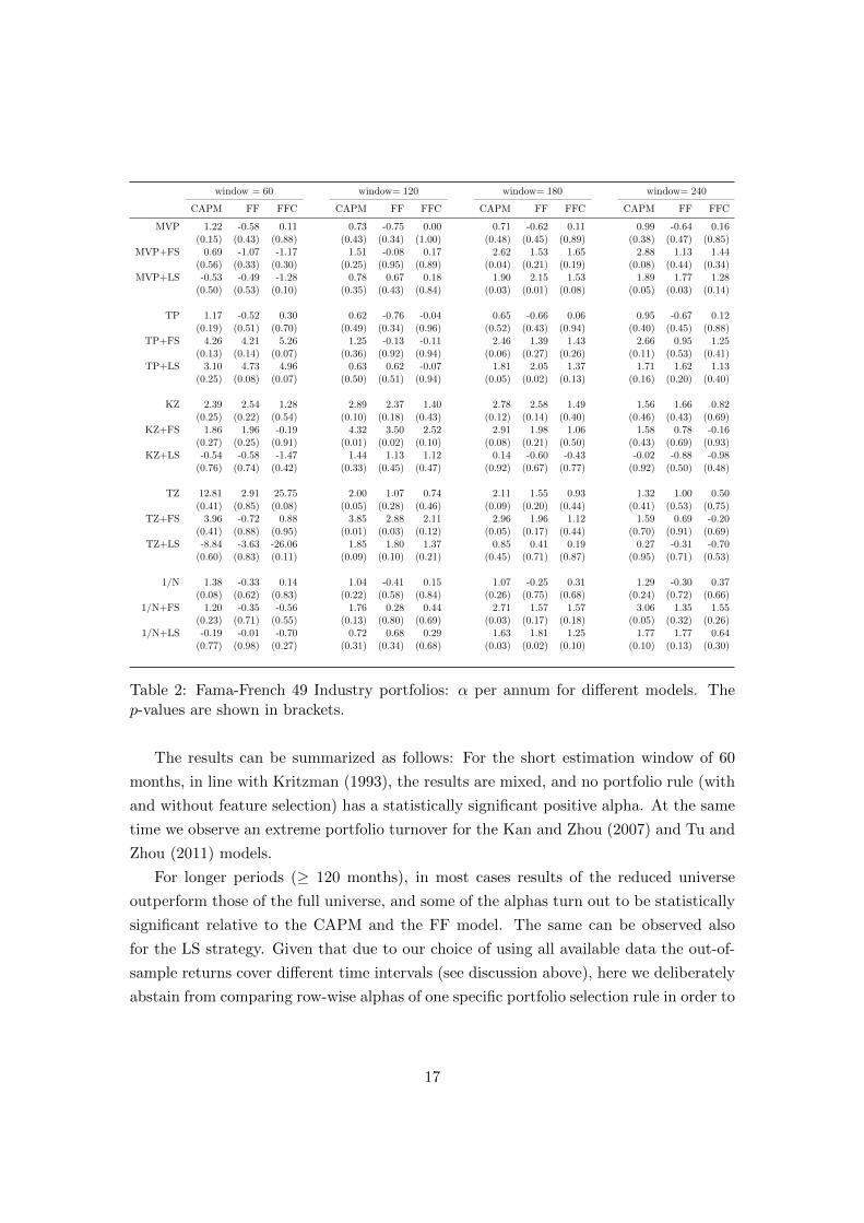
window = 60 window= 120 window= 180 window= 240

CAPM FF FFC CAPM FF FFC CAPM FF FFC CAPM FF FFC

MVP 1.22 -0.58 0.11 0.73 -0.75 0.00 0.71 -0.62 0.11 0.99 -0.64 0.16(0.15) (0.43) (0.88) (0.43) (0.34) (1.00) (0.48) (0.45) (0.89) (0.38) (0.47) (0.85)

MVP+FS 0.69 -1.07 -1.17 1.51 -0.08 0.17 2.62 1.53 1.65 2.88 1.13 1.44(0.56) (0.33) (0.30) (0.25) (0.95) (0.89) (0.04) (0.21) (0.19) (0.08) (0.44) (0.34)

MVP+LS -0.53 -0.49 -1.28 0.78 0.67 0.18 1.90 2.15 1.53 1.89 1.77 1.28(0.50) (0.53) (0.10) (0.35) (0.43) (0.84) (0.03) (0.01) (0.08) (0.05) (0.03) (0.14)

TP 1.17 -0.52 0.30 0.62 -0.76 -0.04 0.65 -0.66 0.06 0.95 -0.67 0.12(0.19) (0.51) (0.70) (0.49) (0.34) (0.96) (0.52) (0.43) (0.94) (0.40) (0.45) (0.88)

TP+FS 4.26 4.21 5.26 1.25 -0.13 -0.11 2.46 1.39 1.43 2.66 0.95 1.25(0.13) (0.14) (0.07) (0.36) (0.92) (0.94) (0.06) (0.27) (0.26) (0.11) (0.53) (0.41)

TP+LS 3.10 4.73 4.96 0.63 0.62 -0.07 1.81 2.05 1.37 1.71 1.62 1.13(0.25) (0.08) (0.07) (0.50) (0.51) (0.94) (0.05) (0.02) (0.13) (0.16) (0.20) (0.40)

KZ 2.39 2.54 1.28 2.89 2.37 1.40 2.78 2.58 1.49 1.56 1.66 0.82(0.25) (0.22) (0.54) (0.10) (0.18) (0.43) (0.12) (0.14) (0.40) (0.46) (0.43) (0.69)

KZ+FS 1.86 1.96 -0.19 4.32 3.50 2.52 2.91 1.98 1.06 1.58 0.78 -0.16(0.27) (0.25) (0.91) (0.01) (0.02) (0.10) (0.08) (0.21) (0.50) (0.43) (0.69) (0.93)

KZ+LS -0.54 -0.58 -1.47 1.44 1.13 1.12 0.14 -0.60 -0.43 -0.02 -0.88 -0.98(0.76) (0.74) (0.42) (0.33) (0.45) (0.47) (0.92) (0.67) (0.77) (0.92) (0.50) (0.48)

TZ 12.81 2.91 25.75 2.00 1.07 0.74 2.11 1.55 0.93 1.32 1.00 0.50(0.41) (0.85) (0.08) (0.05) (0.28) (0.46) (0.09) (0.20) (0.44) (0.41) (0.53) (0.75)

TZ+FS 3.96 -0.72 0.88 3.85 2.88 2.11 2.96 1.96 1.12 1.59 0.69 -0.20(0.41) (0.88) (0.95) (0.01) (0.03) (0.12) (0.05) (0.17) (0.44) (0.70) (0.91) (0.69)

TZ+LS -8.84 -3.63 -26.06 1.85 1.80 1.37 0.85 0.41 0.19 0.27 -0.31 -0.70(0.60) (0.83) (0.11) (0.09) (0.10) (0.21) (0.45) (0.71) (0.87) (0.95) (0.71) (0.53)

1/N 1.38 -0.33 0.14 1.04 -0.41 0.15 1.07 -0.25 0.31 1.29 -0.30 0.37(0.08) (0.62) (0.83) (0.22) (0.58) (0.84) (0.26) (0.75) (0.68) (0.24) (0.72) (0.66)

1/N+FS 1.20 -0.35 -0.56 1.76 0.28 0.44 2.71 1.57 1.57 3.06 1.35 1.55(0.23) (0.71) (0.55) (0.13) (0.80) (0.69) (0.03) (0.17) (0.18) (0.05) (0.32) (0.26)

1/N+LS -0.19 -0.01 -0.70 0.72 0.68 0.29 1.63 1.81 1.25 1.77 1.77 0.64(0.77) (0.98) (0.27) (0.31) (0.34) (0.68) (0.03) (0.02) (0.10) (0.10) (0.13) (0.30)

Table 2: Fama-French 49 Industry portfolios: α per annum for different models. Thep-values are shown in brackets.

The results can be summarized as follows: For the short estimation window of 60

months, in line with Kritzman (1993), the results are mixed, and no portfolio rule (with

and without feature selection) has a statistically significant positive alpha. At the same

time we observe an extreme portfolio turnover for the Kan and Zhou (2007) and Tu and

Zhou (2011) models.

For longer periods (≥ 120 months), in most cases results of the reduced universe

outperform those of the full universe, and some of the alphas turn out to be statistically

significant relative to the CAPM and the FF model. The same can be observed also

for the LS strategy. Given that due to our choice of using all available data the out-of-

sample returns cover different time intervals (see discussion above), here we deliberately

abstain from comparing row-wise alphas of one specific portfolio selection rule in order to

17

Without Feature Selection With Feature Selection Long/Short

T MVP TP KZ TZ 1/N MVP TP KZ TZ 1/N MVP TP KZ TZ 1/N

60 66.0 102.1 1033.1 458.5 38.2 46.9 87.6 179.8 148.7 42.7 184.6 243.4 1236.5 849.2 55.1120 62.6 63.5 581.8 315.6 39.1 41.1 42.0 124.0 102.3 44.5 161.9 188.3 692.3 450.5 56.8180 61.2 61.3 442.6 304.7 39.5 38.3 38.7 98.5 87.6 45.5 153.0 179.3 542.4 417.7 57.4240 61.1 61.1 408.5 307.5 40.9 33.7 34.5 70.5 64.5 49.3 145.6 170.1 472.0 385.8 60.4

Table 3: 49 industry portfolios: Average annual turnover in percentage over the completeback-test period.

find the optimal observation period.11 The indicated turnover for the portfolio selection

rules with feature selection considers the monthly readjustment of the portfolio weights

as well as the annual selection of new representative assets. To summarize, with the

exception of 1/N (where results are similar), applying feature selection on an annual

basis lowers the portfolio turnover. For the Kan and Zhou (2007) and Tu and Zhou

(2011) models this reduction in turnover is remarkable.

Interestingly, we observe this improvement also for the 1/N rule, which is normally

hard to outperform (see e.g. DeMiguel et al., 2009b). We explain this finding by the

avoidance of sector concentration together with choosing low-beta assets. As a support

to this argument, in Table 4 we indicate the beta of the 1/N rule for the whole and

the reduced universes. After selecting only the representative pillars of each cluster, the

beta declines considerably. In this way feature selection relates to the well documented

phenomenon of “betting against beta” of Frazzini and Pedersen (2014).

1/N 1/N+FS

60 months 1.03 0.95120 months 1.01 0.93180 months 1.00 0.89240 months 0.98 0.90

Table 4: 49 Industry portfolios: β of the 1/N rule; with and without feature selection.

As a robustness check, we divide the out-of-sample back-test period into consecutive

10-year periods (the number depends on the observation period) to check whether the

outperformance using feature selection is driven by a few sub-periods with a very large

alpha. Table 5 reports the percentage of 10-year periods in which alpha improves after

using feature selection. It is noteworthy that the majority of test cases show a percentage

well above 50%, i.e. alpha increases after applying feature selection. Again, in line

11When considering only out-of-sample returns of the same time-interval, we found that intermediateestimations windows of 10–20 years perform best. Results are available upon request.

18

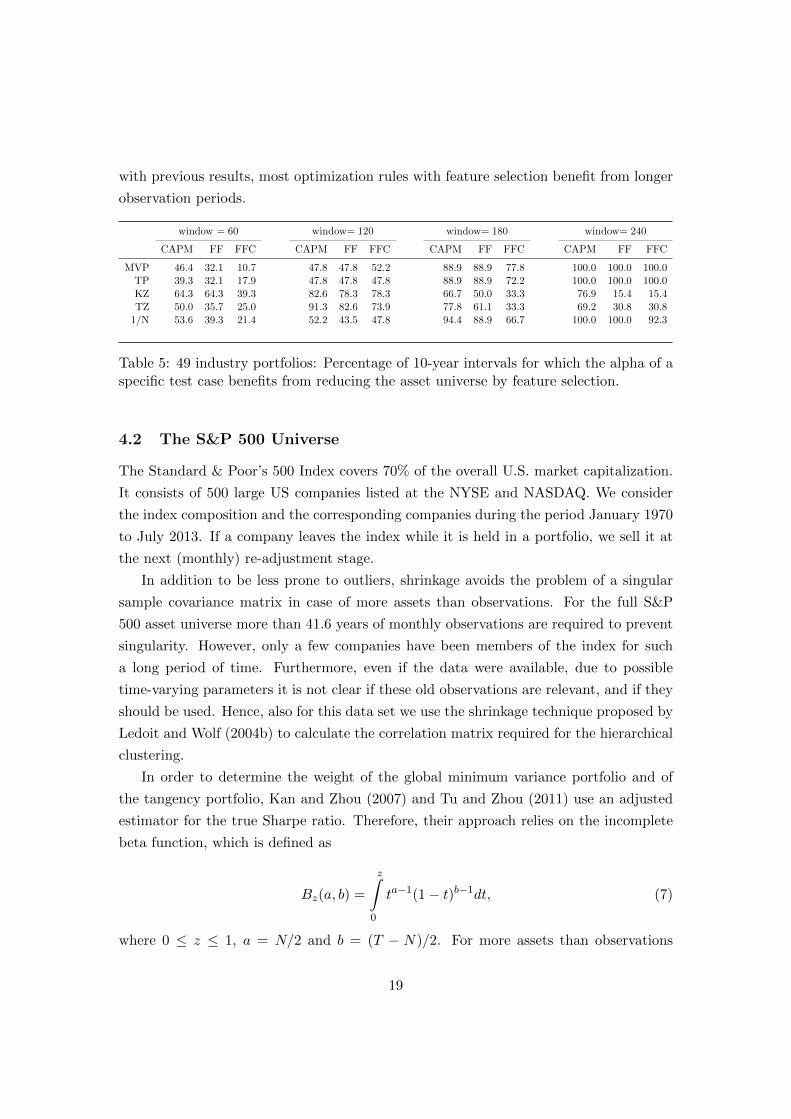
with previous results, most optimization rules with feature selection benefit from longer

observation periods.

window = 60 window= 120 window= 180 window= 240

CAPM FF FFC CAPM FF FFC CAPM FF FFC CAPM FF FFC

MVP 46.4 32.1 10.7 47.8 47.8 52.2 88.9 88.9 77.8 100.0 100.0 100.0TP 39.3 32.1 17.9 47.8 47.8 47.8 88.9 88.9 72.2 100.0 100.0 100.0KZ 64.3 64.3 39.3 82.6 78.3 78.3 66.7 50.0 33.3 76.9 15.4 15.4TZ 50.0 35.7 25.0 91.3 82.6 73.9 77.8 61.1 33.3 69.2 30.8 30.8

1/N 53.6 39.3 21.4 52.2 43.5 47.8 94.4 88.9 66.7 100.0 100.0 92.3

Table 5: 49 industry portfolios: Percentage of 10-year intervals for which the alpha of aspecific test case benefits from reducing the asset universe by feature selection.

4.2 The S&P 500 Universe

The Standard & Poor’s 500 Index covers 70% of the overall U.S. market capitalization.

It consists of 500 large US companies listed at the NYSE and NASDAQ. We consider

the index composition and the corresponding companies during the period January 1970

to July 2013. If a company leaves the index while it is held in a portfolio, we sell it at

the next (monthly) re-adjustment stage.

In addition to be less prone to outliers, shrinkage avoids the problem of a singular

sample covariance matrix in case of more assets than observations. For the full S&P

500 asset universe more than 41.6 years of monthly observations are required to prevent

singularity. However, only a few companies have been members of the index for such

a long period of time. Furthermore, even if the data were available, due to possible

time-varying parameters it is not clear if these old observations are relevant, and if they

should be used. Hence, also for this data set we use the shrinkage technique proposed by

Ledoit and Wolf (2004b) to calculate the correlation matrix required for the hierarchical

clustering.

In order to determine the weight of the global minimum variance portfolio and of

the tangency portfolio, Kan and Zhou (2007) and Tu and Zhou (2011) use an adjusted

estimator for the true Sharpe ratio. Therefore, their approach relies on the incomplete

beta function, which is defined as

Bz(a, b) =

z∫0

ta−1(1− t)b−1dt, (7)

where 0 ≤ z ≤ 1, a = N/2 and b = (T − N)/2. For more assets than observations

19

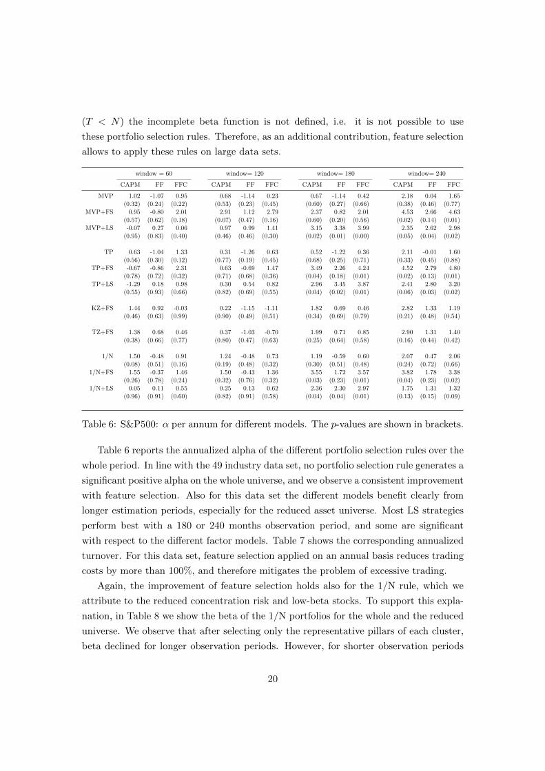
(T < N) the incomplete beta function is not defined, i.e. it is not possible to use

these portfolio selection rules. Therefore, as an additional contribution, feature selection

allows to apply these rules on large data sets.

window = 60 window= 120 window= 180 window= 240

CAPM FF FFC CAPM FF FFC CAPM FF FFC CAPM FF FFC

MVP 1.02 -1.07 0.95 0.68 -1.14 0.23 0.67 -1.14 0.42 2.18 0.04 1.65(0.32) (0.24) (0.22) (0.53) (0.23) (0.45) (0.60) (0.27) (0.66) (0.38) (0.46) (0.77)

MVP+FS 0.95 -0.80 2.01 2.91 1.12 2.79 2.37 0.82 2.01 4.53 2.66 4.63(0.57) (0.62) (0.18) (0.07) (0.47) (0.16) (0.60) (0.20) (0.56) (0.02) (0.14) (0.01)

MVP+LS -0.07 0.27 0.06 0.97 0.99 1.41 3.15 3.38 3.99 2.35 2.62 2.98(0.95) (0.83) (0.40) (0.46) (0.46) (0.30) (0.02) (0.01) (0.00) (0.05) (0.04) (0.02)

TP 0.63 -1.04 1.33 0.31 -1.26 0.63 0.52 -1.22 0.36 2.11 -0.01 1.60(0.56) (0.30) (0.12) (0.77) (0.19) (0.45) (0.68) (0.25) (0.71) (0.33) (0.45) (0.88)

TP+FS -0.67 -0.86 2.31 0.63 -0.69 1.47 3.49 2.26 4.24 4.52 2.79 4.80(0.78) (0.72) (0.32) (0.71) (0.68) (0.36) (0.04) (0.18) (0.01) (0.02) (0.13) (0.01)

TP+LS -1.29 0.18 0.98 0.30 0.54 0.82 2.96 3.45 3.87 2.41 2.80 3.20(0.55) (0.93) (0.66) (0.82) (0.69) (0.55) (0.04) (0.02) (0.01) (0.06) (0.03) (0.02)

KZ+FS 1.44 0.92 -0.03 0.22 -1.15 -1.11 1.82 0.69 0.46 2.82 1.33 1.19(0.46) (0.63) (0.99) (0.90) (0.49) (0.51) (0.34) (0.69) (0.79) (0.21) (0.48) (0.54)

TZ+FS 1.38 0.68 0.46 0.37 -1.03 -0.70 1.99 0.71 0.85 2.90 1.31 1.40(0.38) (0.66) (0.77) (0.80) (0.47) (0.63) (0.25) (0.64) (0.58) (0.16) (0.44) (0.42)

1/N 1.50 -0.48 0.91 1.24 -0.48 0.73 1.19 -0.59 0.60 2.07 0.47 2.06(0.08) (0.51) (0.16) (0.19) (0.48) (0.32) (0.30) (0.51) (0.48) (0.24) (0.72) (0.66)

1/N+FS 1.55 -0.37 1.46 1.50 -0.43 1.36 3.55 1.72 3.57 3.82 1.78 3.38(0.26) (0.78) (0.24) (0.32) (0.76) (0.32) (0.03) (0.23) (0.01) (0.04) (0.23) (0.02)

1/N+LS 0.05 0.11 0.55 0.25 0.13 0.62 2.36 2.30 2.97 1.75 1.31 1.32(0.96) (0.91) (0.60) (0.82) (0.91) (0.58) (0.04) (0.04) (0.01) (0.13) (0.15) (0.09)

Table 6: S&P500: α per annum for different models. The p-values are shown in brackets.

Table 6 reports the annualized alpha of the different portfolio selection rules over the

whole period. In line with the 49 industry data set, no portfolio selection rule generates a

significant positive alpha on the whole universe, and we observe a consistent improvement

with feature selection. Also for this data set the different models benefit clearly from

longer estimation periods, especially for the reduced asset universe. Most LS strategies

perform best with a 180 or 240 months observation period, and some are significant

with respect to the different factor models. Table 7 shows the corresponding annualized

turnover. For this data set, feature selection applied on an annual basis reduces trading

costs by more than 100%, and therefore mitigates the problem of excessive trading.

Again, the improvement of feature selection holds also for the 1/N rule, which we

attribute to the reduced concentration risk and low-beta stocks. To support this expla-

nation, in Table 8 we show the beta of the 1/N portfolios for the whole and the reduced

universe. We observe that after selecting only the representative pillars of each cluster,

beta declined for longer observation periods. However, for shorter observation periods

20

Without Feature Selection With Feature Selection Long/Short

T MVP TP KZ TZ 1/N MVP TP KZ TZ 1/N MVP TP KZ TZ 1/N

60 313.0 356.1 71.2 130.6 152.3 173.9 141.6 69.4 427.9 501.3 136.0120 260.5 285.0 71.0 117.2 120.0 132.7 117.0 68.1 364.9 391.2 134.1180 234.9 252.1 69.0 109.2 113.0 118.5 107.7 65.9 332.4 353.7 129.4240 202.6 211.8 68.5 90.3 93.1 92.6 87.4 63.7 282.9 294.5 125.9

Table 7: S&P500: Average annual turnover in percentage over the complete back-testperiod.

we could not observe this reduction in beta. Given the higher number of individual

assets (compared to the 49 portfolios in the previous data set), we attribute this fact

to a more severe parameter estimation problem. A more thorough investigation of the

effect of feature selection on the beta of a portfolio is left to future research.

1/N 1/N+FS

60 months 1.06 1.07120 months 1.02 1.02180 months 1.00 0.97240 months 0.99 0.95

Table 8: S&P500: β of the 1/N rule; with and without feature selection

window = 60 window= 120 window= 180 window= 240

CAPM FF FFC CAPM FF FFC CAPM FF FFC CAPM FF FFC

MVP 50.0 60.7 78.6 65.2 78.3 78.3 100 94.4 100 92.3 84.6 84.6TP 57.1 57.2 75.0 65.2 78.3 78.3 100 94.4 100 92.6 84.6 84.6

1/N 64.3 64.3 75.0 60.9 78.3 52.2 100 94.4 94.4 84.6 76.6 76.6

Table 9: S&P500: Percentage of 10-year intervals for which the alpha of a specific testcase benefits from reducing the asset universe by feature selection.

Table 9 shows the percentage of 10-year periods in which alpha increases with feature

selection. Here we can clearly see that longer estimation periods improve the results of

feature selection, especially for 15 and 20 years.

5 Conclusion

Parameter uncertainty is a major cause for the poor out-of-sample performance of port-

folio selection rules based on the sample mean and the sample covariance matrix. We

21

propose reducing the asset universe with hierarchical clustering before applying the port-

folio selection rule. To assess the benefits of our proposal with out-of-sample back-tests,

we apply five well-established portfolio selection rules with different estimation windows

on two different data sets: the Fama-French 49 industry portfolios and the constituents

of the S&P 500 index. For most test cases, alpha relative to different prominent factor

models is improved by using feature selection, and some alphas are statistically signifi-

cant. We apply a robustness check to show that our results are not driven by a couple

of return outliers. Furthermore, in some cases with longer estimation windows also the

alpha of a long/short strategy turns out to be statistically significant. We consider this

finding to be in support of the proposed approach. Finally, our method mitigates the

problem of excessive portfolio turnover.

Acknowledgements

We thank Michael Hanke, Kourosh Marjani Rasmussen, the Guest Editors Nalan Gulpinar,

Xuan V. Doan and Arne K. Strauss, and two anonymous referees for helpful comments.

Special thanks also to conference participants of the APMOD 2014 at the University

of Warwick and seminar participants at the University of Oxford and the Technical

University of Denmark.

22

References

Best, M. J. and Grauer, R. R. (1991). On the Sensitivity of Mean-Variance-Efficient

Portfolios to Changes in Asset Means: Some Analytical and Computational Results.

Review of Financial Studies, 4(2):315–342.

Black, F. and Litterman, R. (1992). Global Portfolio Optimization. Financial Analysts

Journal, 48(5):28–43.

Carhart, M. M. (1997). On Persistence in Mutual Fund Performance. The Journal of

Finance, 52(1):57–82.

Chopra, V. K. and Ziemba, W. T. (1993). The Effect of Errors in Means, Variances,

and Covariances on Optimal Portfolio Choice. The Journal of Portfolio Management,

19(2):6–11.

Clarke, R. G., de Silva, H., and Thorley, S. (2006). Minimum-Variance Portfolios in the

U.S. Equity Market. The Journal of Portfolio Management, 33(1):10–24.

DeMiguel, V., Garlappi, L., Nogales, F. J., and Uppal, R. (2009a). A Generalized Ap-

proach to Portfolio Optimization: Improving Performance by Constraining Portfolio

Norms. Management Science, 55(5):798–812.

DeMiguel, V., Garlappi, L., and Uppal, R. (2009b). Optimal Versus Naive Diversifi-

cation: How Inefficient is the 1/N Portfolio Strategy? Review of Financial Studies,

22(5):1915–1953.

DeMiguel, V. and Nogales, F. J. (2009). Portfolio Selection with Robust Estimation.

Operations Research, 57(3):560–577.

Duchin, R. and Levy, H. (2009). Markowitz Versus the Talmudic Portfolio Diversification

Strategies. The Journal of Portfolio Management, 35(2):71–74.

Fama, E. F. and French, K. R. (1993). Common Risk Factors in the Returns on Stocks

and Bonds. Journal of Financial Economics, 33(1):3–56.

Frazzini, A. and Pedersen, L. H. (2014). Betting Against Beta. Journal of Financial

Economics, 111(1):1–25.

Hartigan, J. A. (1981). Consistency of Single Linkage for High-Density Clusters. Journal

of the American Statistical Association, 76(374):388–394.

23

Haugen, R. A. and Baker, N. L. (1991). The Efficient Market Inefficiency of

Capitalization-weighted Stock Portfolios. The Journal of Portfolio Management,

17(3):35–40.

Jagannathan, R. and Ma, T. (2003). Risk Reduction in Large Portfolios: Why Imposing

the Wrong Constraints Helps. The Journal of Finance, 58(4):1651–1684.

Jorion, P. (1986). Bayes-Stein Estimation for Portfolio Analysis. The Journal of Finan-

cial and Quantitative Analysis, 21(3):279–292.

Kan, R. and Zhou, G. (2007). Optimal Portfolio Choice with Parameter Uncertainty.

Journal of Financial and Quantitative Analysis, 42(03):621–656.

Kritzman, M. (1993). What Practitioners Need to Know. . . About Factor Methods.

Financial Analysts Journal, 49(1):12–15.

Kritzman, M., Page, S., and Turkington, D. (2010). In Defense of Optimization: The

Fallacy of 1/ N. Financial Analysts Journal, 66(2):31–39.

Ledoit, O. and Wolf, M. (2003). Improved Estimation of the Covariance Matrix of Stock

Returns with an Application to Portfolio Selection. Journal of Empirical Finance,

10(5):603–621.

Ledoit, O. and Wolf, M. (2004a). A Well-conditioned Estimator for Large-dimensional

Covariance Matrices. Journal of Multivariate Analysis, 88(2):365–411.

Ledoit, O. and Wolf, M. (2004b). Honey, I Shrunk the Sample Covariance Matrix. The

Journal of Portfolio Management, 30(4):110–119.

Ledoit, O. and Wolf, M. (2012). Nonlinear Shrinkage Estimation of Large-dimensional

Covariance Matrices. The Annals of Statistics, 40(2):1024–1060.

Levy, H. and Levy, M. (2014). The Benefits of Differential Variance-based Constraints in

Portfolio Optimization. European Journal of Operational Research, 234(2):372–381.

Lisi, F. and Corazza, M. (2008). Clustering Financial Data for Mutual Fund Manage-

ment. In Perna, C. and Sibillo, M., editors, Mathematical and Statistical Methods in

Insurance and Finance, pages 157–164. Springer Milan.

Markowitz, H. (1952). Portfolio Selection. The Journal of Finance, 7(1):77–91.

Merton, R. (1980). On Estimating the Expected Return on the Market: An Exploratory

Investigation. Journal of Financial Economics, 8:323–361.

24

Nanda, S., Mahanty, B., and Tiwari, M. (2010). Clustering Indian Stock Market Data

for Portfolio Mnagement. Expert Systems with Applications, 37(12):8793–8798.

Scherer, B. (2011). A Note on the Returns from Minimum Variance Investing. Journal

of Empirical Finance, 18(4):652–660.

Tan, P.-N., Steinbach, M., and Kumar, V. (2006). Introduction to Data Mining. Pearson.

Tobin, J. (1958). Liquidity Preference as Behavior Towards Risk. The Review of Eco-

nomic Studies, 25(2):65–82.

Tola, V., Lillo, F., Gallegati, M., and Mantegna, R. N. (2008). Cluster Analysis for

Portfolio Optimization. Journal of Economic Dynamics and Control, 32(1):235–258.

Tu, J. and Zhou, G. (2011). Markowitz meets Talmud: A Combination of Sophisticated

and Naive Diversification Strategies. Journal of Financial Economics, 99(1):204–215.

Xu, R. and Wunsch, D. (2005). Survey of Clustering Algorithms. IEEE Transactions

on Neural Networks, 16(3):645–78.

25