- 7,

JR. LYANI-ALLEN--

FEBRUAR"I 19729

- ~Techiafl Report ERI"M-23

ANl INCREM ENT,"lA L V E LOCIT YMEASUREMENT ALGOURITH FOR US'E

* i INRTIL NAVIGAT ION ALIGNM"FENT

OFFI1CE OF NAVAL- RESEA.RCZý INFOPMATION SERVICE

DEC0AWTMN4-OF THE NAVY '

WASHNG-TON D C 20360 - .U

This documenthnw been apoved firpub&k rdJs~and wzle. Ut &fce utnibuon ij 'jni&itef

E~d Prelect'71 21-s

Unclassified

DOCUMENT CONTROL DATA - R &D

Engineering Research Institute I UnclassifiedIowa State University

Ames, Iowa 50010

AN INCREMENTAL VELOCITY MEASUREMENT ALGORITHM FOR USE IN

INTERNAL NAVIGATION ALIG*4NTT

Technical Report, February 1972* '.-.ons ,S , 'P- nam. reddl. mmhla* It ga'. .

R. L. VanAllen and R. G. Brown

February 1972 I /0

N00014-68-A-0162h ,P-o•C T 1,0o ISU-ERI-AMES-72023

ERI 712-SI is ZPO . '. thaF fN" t- ~.-tn,

dm

This document is approved for public release and sale: its distributionis unlimited

Office of Navai ResearchDepartment of the NavyWashington, D.C. 20360

In any inertial navigation system the platform must be initially aligned insome known frame of reference prior to operation in the navigation mode. Self-alignment methods are preferred in most applications, and the usual procedure isto align the platform locally level with one accelerometer axis pointing north.In the current generation of aircraft inertial systems the sensed acceleration isin the form of incremental velocity pulses. These are accumulated to yield a measureof total velocity within the granularity of the incremental velocity change. Kalmanfiltering techniques have recently been applied to the alignment problem, the usualmode of operation samples the total velocity at a fixed rate, and the resultingsequence of samples becomes the input to the Kalman filter. Granularity in thevelocity measurement is then treated as uncorrelated measurement noise.

"A new approach to the alignment problem is considered in this report wherebythe incremental velocity pulses are modeled directly as the measurement sequence.This leads to three important changes in the filter model: (1) aperiodic sampling

is obtained; (2) measurement noise due to granlarity is eliminated; an-4.") adelayed state appears in the measurement equati'n. This latter condition forces theuse of a modified form of the Kalman recursive equations. Rcsults of Monte Carlosimulaticns ior one set of noise parameters are given. Ihese indicate that con-sidera'ýe improvement in perfc-rmance may be expected from this technique relative

to the more conventional -ode.ing technique.

DD (PAGE 1) Uncasified

Unclassifiedz .¢Security Ci,..fxd atlon

'4LINK ALI K SLN CI

-1II I I - - II-I

S_ T O tE my

Navigation

Inertial Navigation

Kalman filter

Inertial alig-ament

I:I

* 'I

FORM U. tm. .m IIDD, "w6911473nBACe! N~ IS .. •:.. •:,Unclassified

ENGINEERINGRESEARCHENGINEERINGRESEARCHENGINEERINGRESEARCHENGINEERINGRESEARCHENGINEERINGRESEARCH

TECHNICAL REPORT

AN INCREMENTAL VELOCITYMEASUREMENT ALGORITHM FOR USEIN INERTIAL NAVIGATION ALIGNMENT

R. L. VanAInR.G. Brow.

Febtuay 1972

ce"-w! & "java. R0 .eea'c- iPe i -na' may tin! rnrh*fb flt tt.,f lZ1ite

tDenal-- of menar.. ol Ith United slaunThe.ns, Contract .*00014-68-A 0162

ENGINEERING RESEARCH INSTITUTEERIProlect 712-S IOWA STATE UNIVERSITY AMES

ABSTRACT

In any inertial navigation system the platform must be initially

aligned in some known frame of reference prior to operation in the

navigation mode. Self-alignment methods are preferred in most appli-

cations, and the usual procedure is to align the platform locally level

with one ac:elerometer exis pointing north. In the current generation

of aircraft inertial systems the sensed acceleration is in the form

of incremental velocity pulses. These are accurlated to yield a

measure of total velocity within the granularity of the incremental

velocity change. Kalman filtering techniques hbae reci-tly been applied

to the alignment problem, the usual mode of operation samples the total

velocity at a fixed rate, and the resulting sE-uence of samples becomes

the input to the Kalman filter. Granularity in the velocity weaure-

ment is then treated a- uacorrelated measurement noise.

A new approach to the alignment problem is considered in this

report wihereby the incremental velocity pulses are modeled directli as

the measurement sequence. This leads to three important changes in

the filter mo.el: (1) aperiodic sawpling is obtained: (2) measurement

noise due to granularity is eliminated; and (3) a delayed state appears

in the measurement equation. This latter condition forces the use of

a modified form of t,4,e Kal!an recursive equations. Results of Monte

Carl- simulations for one set of noise parameters are given. These indi-

cate that c¢nsiderable improvement in performance may be expected from.

this technique relative to the mcre conventional modeling tecnnique.

TABLE OF CONTENTS

Page

I. INTRODUCTION 1

Il. KALMAN RECURSIVE EQUATIONS 3

III. MATHEMATICAL MODELS 6

A. System Dynamics and Incremental Velocity 6Measurement Model

B. Incremental Time Measurement Model 20

IV. DIGITAL SIMULATION 23

A. Method of Analysis 23

B. Process and Measurement Simulation 23

C. Delta Velocity Kalman Estimator 30

D. Time Interval Kalman Estimator 34

E. HPHI Subroutine 34

V. RLSULTS 37

Vi. CONCLUSIONS 48

VII. LITERATURE CITED 49

VIII. AC.NOWLEDGEMENTS 50

IX. APPENNDIX A: SIMULATION PROGRAM 51

A. Main Program 51

B. DVWAL Subroutine 58

C. TII-AL Subroutine 62

D. HPHI Subroutine 66

X. APPENDIX B: GRAPHICAL RESTU"TS 70

A. Azimuth Error 70

B. Level Tilt 81

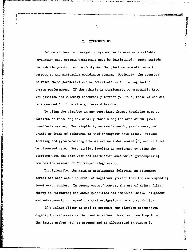
1. INTRuDUMtKIt

Before an inertial navigation system can be used as a reliable

navigation aid, certain qu.antities must be initialized. These include

the vehicle position and velocity and the platform orientation with

respect to the navigation coordinate system. Oviously, the accuracy

tc which these parameters can be determined is a limiting factor in

system performance. If the vehicle is stationary, we presumably know

its position and vAocity essentially perfectly. Thus, these values can

be accounted for in a straightforward fashion.

To align the platform in any coorainate frame, knowledge must be

5*tainec. of three angles, usually those along the axes of the given

coordinate system. For simplicity an x-a.is north, y-axis west, and

L-axis up frame of reference is used throughout this paper. Various

leveling and gyrocompassing schemes are well documented ! I, and will not

be discussed here. Essentially, leveling is performed to align the

platform with the east-west and north-south axes while gyrocompassing

reduces the azimuth or "north-pointing" error.

Traditionally, the azimuth misalignment following an alignment

period has been about an order of magnitude greater than the corresponding

level error angles. In recent ,,ears, however, the use of Kalmsn filter

theiry in iEstimating the above quantities has improved initial aligr=ent

and subsequently increased inertial navigatior accuracy capability.

If a Kalman filter is usei to estimace the platform orientation

angles, the estimates can be used in either closed or open loop form.

The latter method will be assumed and is illustrated in Figure 1.

2

Inertial Navigation

Vehicle System Kalman Platform

Dynamics (including Gyros and FilterF• Misorientation

Accelerometers) Angles

Figure 1. Open loop estimaticn

in this scheme output from the inertial navigation instrument cluster is

processed in the Kalman filter for some predetermined alignment time. At

the end of the alignment interval, platform correctior. information pro-

portional to the misalignment angles is used in the to::-uer motors to

correct any platform misorientation.

In this paper a gyrocompassing technique using a new and unique

incremental velocity measurement algorithm in a Kalman filter estimation

scheae is presented and compared with a system employing a somewhat

standard time inteýrval measurement method with simple periodic sampling.

3

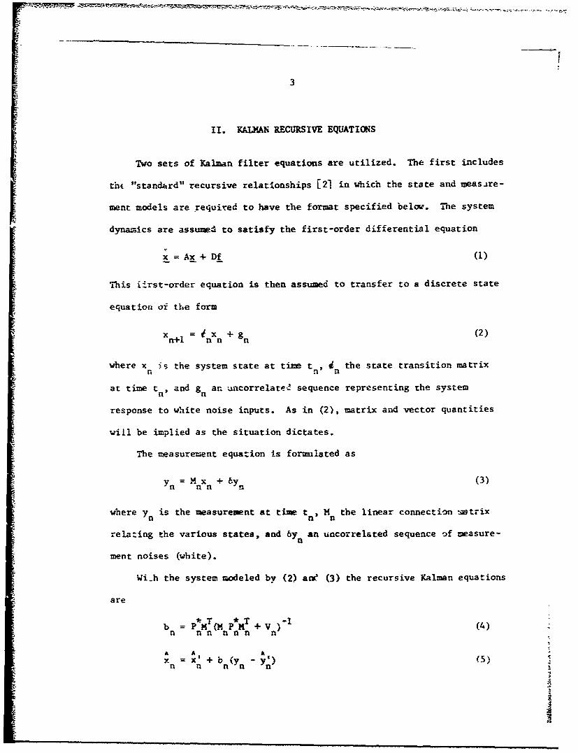
II. KALMAN RECURSIVE EQUATIONS

Two sets of Kalman filter equations are utilized. The first includes

th* "standard" recursive relationships [21 in which the state and measire-

ment models are required to have the format specified below. The system

dynamics are assumed to satisfy the first-order differential equation

x = Ax + Df (1)

This iirst-order equation is then assumed to transfer to a discrete state

equation of the form

X n+l inX + gn (2)

where x 5s the system state at time t n, the state transition matrixn n

at time tn, and g n an ancorrelate,2 sequence representing the system

response to white noise inputs. As in (2), matrix and vector quantities

will be implied as the situation dictates.

The measurement equation is formulated as

Yn = M nxn + 6y (3)

where yn is the measurement at time t, Mn the linear connection wtrix

rela:ing the various states, and 6yn an uncorrelated sequence of measure-

ment noises (white).

Wi.h the system modeled by (2) ane (3) the recursive Kalman equations

are

bn P p MTn + V) (4)

A A Ax' + b ny - y') 5)n n n n n

4

P= P bn(HnPnMn T V)b (6)

A A'+ 'm x n(7)Xn+l n n

Pn-i- an=6?+n (8)

where 6 = transition matrix for interv-al from t to tn+1

x = trae state at time tn n

Ax = optimum a posteriori estimate of x at time t

Ax' = optimum a priori estimate of x at :_ime t

n n

b = gain matrixn

v = measurement at time t

A Ay =Mx

n n nA

= covariance matrix .)f the estimation error (x' - x )n n n

A

P = covariance matrix of the estimation error (x - xna n"

M = measurement matrixn

V covariance matrix of the measurement error, i.e.,n

SVn = E(ýy T)nl II n

H = covariance matrix of the response of the states to alln

Twhite noise drivirg functions, i.e., H. E(g ngn)

Lt = time increment between tn and t +1

The other set of recursive equations used involve the use of a

modified (delayed-state) measurement model. The measurement equation is

Yn = M x + N x + (9)n an nan-i aY

That is, the measurement at time t consist= of a linear connection ton

states at both t and t . As before, the system is described by (2).staesatboh n tnI.

In this configuration the recursive relationships become [i3iJ

b = (PM + P N)Q (10)rt n r n-i n-i1n

A A AX = x' + bn(Y Y) (11)

n n n n n

P = P -bQb (12)n n nn

A, A (13)

n+l Tnn

*p T + H (14)'n+l = n n n n

where

lkjT .T TTQ= (MP'1 +V) +I p N + 'iP 0 +M P NT

= n n n n n n-1 n n n-1 n-i n n n-i n-1 n

(15)

and

A A A

"' =MX' + NX 1 (16)

A derivation of the above delayed-state equations in included in the

Appendix of [F4.

6

III. MATHEMATICAL MODELS

A. System DynarsIcs and Incremental VelocityMeasurement Model

The following development of the system dynamics is essentially

included in Pitman [L] while the incorporation of the new increwentul

velocity measurameat algorithm is taken largely from unpublished notes

by Dr. R. G. Brown of Iowa State University.

The basic equations that describe the inertial system error propaga-

tion for a stationary vehicle are

Sv -zy =x (17)

Equations ty + " -4 =e (18)

'z + x X C z (19)

"266 + -z 6e + W (60 + Vy 6a /R (20)

Schuler y z x 0 y + x

Dynamics 2"L 205ý 5 M - Z6' + w (60 +x)=- 6a /R (21)x z y o x Xy

where

ix ,Y6' 6 = actual platform coordinate frame errors

* 89 69 , 69 = computer coordinate frame errors

-69

A'x, 44 y' ,z = angular earth rate components along the

x, y, and z axes respectively

'Ex, Cy, Cz = gyro drift rsce (bias) errors

Fa 8a = accelerometer bias errorsx y

7

R = radius vector from the center of the

earth to •rue vehicle position2w 2 local gravity vector, g, divided by the

0

earth radius vector, R

The above angles are illustrated in Figure •'

Z* Z' ~x, y, z = Ideal coordinate

(up) system

x', y', z' = Actual platformcoordinates

x*, y*, z* = Computer platformcoordinates

-y*

y (west)

x ZI i

(north) 0. I

Figure 2. Coordinate system relationships

It should be noted that a third Schuler equation involving 60 is notz

included because the vertical error is assinmd to be zero. IThe physical quantities that we desire to estimate in our Kalman

filter are the level tilts (4 and 6 ) and azimuth e:ror (6 ). Thesex y z

angles can be inserted into the system equations through the relation

2A

8

6 = * + 60. The effect of knowing position perfectly is that 69 = 0.

Thus, an = j and (17), (18), and (19) become

'x -r y (22)

6 +z•6 -C = (23)y z x x z y

+ 6 =C_ (24)z x y

For the purposes of this study we make several simplifying assump-

tions. We first assume that so-e sort of coarse aligrment has taken

place such that the level tilts are relatively small as compared with

aziumuth error (statistically, at least). Also we let the gyro drifts and

accelerometer biases be zero (i.e., we assume perfect instruments).

Then (22), (23), and (24) become

x 0 (25)x

; -Ai '6 0 (26)y x z

Z6• 0 (27)

An explicit solution can now be written for 6 X 6y' and 6z"

ix(t) = 6x (0) (28)

() = 6 z(0) (29)z

tS(t) = aQ 6dt + 1 (0)y ' xz y

0

= 6 6 (O)t +•6 (0) (30)x z y

or

9I

1 0 0 46 (0)x xzero

4y = 0 1 0Oxt Ay (0) + driving (31)

0 0 1 0function

L zL0 J -0

These, then, are the ba3ic state equations.

The measurement model must take into account the "real-world"

accelerometer mechanization. Basically the accelerometer emits a pulse

nhe.ever a predetermined increment in velocity (integrated acceleration)

is reached. Physically this can take the form of an integrator at the

acceleuoz-eter output. The integratcr is used in; conjunction with a

threshold detector that emits a + LV pulse whenever the preset threshold

is reached. When the delta velocity pulse is emitted, the appropriate

positive or negative LV increment is fed back, ideally resetting the

integrator to zero. An example of an integrated acceleration functior

and the corresponding sequence of LV pulses is shown in Figure 3.

IntegrztedAcceleration

tIt 2 t 3 * Time

Accelerometer V ' [

igtput tegrted cl in Tio e

Figure 3. Integrated acceleration function

K10

Note the nonuniform time interval between pulses.

Using the open-loop correction scheme dihcussed ..bove, we want to

estimate the level tilts (6 6) and the azimuth error (6) based on

a sequence of AV measurements that occur in a finite interval of time.

Explicitly the LAV measurement is (for both accelerometers)

tn

a (t)dtt n -1I

andt

na (t)dt

x y

Now

ax g6 -gy + (Noise) x (32)

a= g6x + (Noise) (33)

y y

Using (31), (32), and (33) the problem decouples as foll s

6 6 (0) Process Modelx xEast-West i

Nort'h-South I6 I 1o 0 roes HdCiar-nel _3z 0 1 6 [.(O)

I = gi + (Noise) Measurementy x

At this point we will d_!velop only the north-south measurement equations

as that channel furnishes the informtion concerning azimuth error. The

east-west derivation proceeds in an analagous fashinn and will be

omitted.

The actual measuremnt is

t

a dtl-n-l

Writing this out explicitly we obtain (from (32)),

t t tn n n

a X(t)dt - gi (t)dt + noiset n-I t n-I t n-I

Substituting for 6 (t),

t t tn n n

a (t)dt=- g ( [i (O)t + 4(O))dt+ noiseSx: ytn-1 tn-1 tn_1

P- . A (0)(t •- t2_ -g6(o)(t -X z n n- y n n-I

t

n noise (34)

tn-1

NOW Subst ituting

y (0) = 6 (t) -0 xz t

= (t)) 6 ty n x zn

and 6 (0) 6 (t ) into (34) we obtainz n

a (t)dt=- g)(t 2-t 2 -g (t 04)6t )(t t )x xz n n-i y a X n n-iSt n-i t

+ noise (35)

tn-l

12

Rearranging (35)

tr• n

>>J t a x (t)dt TMg 0 x z (t n t n-1 t n n+t n-1 )J

Sn-L t ngy(t )(t t + noise (36)

J tx- xzt

Nc let t - = n At . Then

tn 2

ax(t)dt = ( g At2n)4 z( tn) + (- n t)y(tn)tnI ttn I+ Itn noise

(37)

n1-1

Equation (37) is now in the correct measurement format except for the

noise term.

To account properly for the integrated noise tern in (37), let us

assune that the major source of noise is random lateral motion of the

vehicle plus white instrumnt noise. Although lateral notion was ignored

in the systen process derivation, it is an important noise source due

to wind buffetirg, loading, and gt.-eral random motions that occur to the

vehicle. In deriving our noise model we will let the vehicle be an

aircraft, thus knowing that there is no appreciable net random motion

(position) when it is stationawy on the ground. At the acceleration

level this is a special type of noise; it is such that the double integral

of the acceleration noise is bounded, and is thus a stationary process.

Therefore, let us asst.w that at the position level, the process is

shaped .arkov. Then, so that acceleration and velocity have bounded

variance, w-e postulate the model shown in Figure 4 (position that is

13

Markov shaped by a secored-order filter). Note that position, ve!ocity,

Unity 2-AccelerationWhite r_______ NoiseNoise n1(7N

sf -3 J2nlt

position

Figuire 4. Noise model

2.and ac :eleration all have bounded variance- with the parameters j 5, >

Xrand r chosen to fit the physical situation at hand.

The second part of the integrated noise term~ is the con-tribution

due to instru-ment noise. This noise is assured to arise from the basic

acceleren'eter itself (e.g., proof mass jitter due to noise from the

serVo electronics) and thus appears as integrated acceleratic-n noise

at the instr=u-nt output. We will assume that the basic acceleration

noise i3 white, thus the acceleromter output is a random valk process

as shown in Figure 5. K1 is choasen to fit the physical situation.

The randon walk process is described b~y the first-order differential

equation

n2(t) =v(t) (33)

lategrating, we obtain

i, (t) n 2(0), + h(t)(Driven Response) (39)

14

or in difference equation format

n =n + h (40)n+l 2 n

where h is found by forming the convolution integrz1 [510

ist

hn J y(u)v(-t-u)du (41)0

y(u) is the weighting fuaction of the filter (i.e., the inverse Laplace

transform of l/s),

Instrumnt Noise Acceleration NoiseV(t) n2(t)

(white noise-amplitude tn)

Figure 5. Instrunent noise random process

Y(u)= ls) (42)

"Then

h 1-v(bt-u)iu = 0 (43)n J

0

since the white noise input v(t) has zero mean. Also,

At £1th2 -h 2 y(u)y(w)v(At-w)v(ý,t-u)dudw (44)

0 0

and At AtSh2 . . -5

h n= y(u)y(v)v(•-tu)v(Lt-w)dudw (45)

0 0

15

Since v(t) is white noise with amplitudeK1 , v(t-u)v(t-w) K -N (u-w).

where 5( ) is the Dirac delta function. Trhen

L"t At

hn . (-4-6)6u-w~du&; ( 6

0 0

Using sifting integral theory,

Lt

h 2 = IdS -1K

0

= K 1t (47)

Thus h can be represented by an uncorrelated sequence of Gaussian randomn

variables with zero mean and variance equal to K lt.

Let us now assign states to the physic;,l quantities to obtain the

correct process model format for r.e Ka mar filter. Let

xi = 6 ( 48)

x2 = z (49)

Figure I' can be redrawn as

2 AccelerationNoise

I, 2 2

(Unity (s + *)(s + 2w • s W r) z(t) Noise

White _____________ __

Noise , 1- PositionNoise

Figure 6. State formulation of noise model

i

3

16

Now let

x4 = z(t) (position noise) (50)

x4 = z(t) (velocity noise)

x (t) (acceleration noise) (52)

The basic differential equation is

2 2-(5 + 2Cw r) + Ur + 2w )z +5u z = f(t) (53)

Then in matrix form we have

x3 0 1 0 x3

x 4 0 0 1 x4

2 2 u -(5+2rCL r r r -+2r L 5

F 0+ 0 (54)

W r .B'• f(t) (5J

Equation (54) is in the standard state variable form of Equation (1).

Thct state transition matrix can now be found in closed form from

[(t) =t'E(sI - A)-l (55)

where I is the identity iatrix. Each term of 6(t) is of the form

Kie e + Lij e rsin (Wr + j) (56)

& 17

2where K L and 9.. are functions of . ," , and .

Tie driven responses for the states (gn) can be found in closed

form by again forming the convolution intiegral

t

x.(t) = y•i(u)f(t-u)du (57)2. 1

0

where yi (u) is the weighting function between f(t) and the state of

interest, x.. Then

t

x.(t) = = (u)f(t-u)du 0 (58)0

nndt t

x 2(t)- yM(u)y(v)f(t-,i)f(t-v)dudv (59)0 0

2

as before. x2(t) again indicates taking the expect.:d value. Since f(t)

is unity variance white noise, f(t-u)f(t-v) is just 6(u-v). Equation (59)

then becomes

t t2

x.(t) = - Yi(u)yi(v)5u-v)dudv (60)1

0 0

-2 (v)dv (61)

0

T-hus the driven response for cach state, xi, is a random variable with

t-2

zero mean and variance equal to y (v)dv, where we let t = at.

0

18

Recapping, then,

X (3,3) ] "3

,5,5)II Inx+l (Transition + g4

Matrix)

"xS n+lL x5 g5n n

The last state to be considered is described by (40). Here we let

n2 = x6 and hn = 96 " Thu.n n nF x = x6 + g6 (62)

n+l n n

Finally, combining all six states in matrix form,

i . Lt 0 0 00 rx0

0 1 0 0 0 0 0

0 0= n0(3,3) 1 x + n (63)

0 0 : through iO -n4 n0 0 6 (5,-)10 9

L I n0 0 0 0 0 g6

The process model is now in the correct format.

Returning to the measurement equation, (37), we now write

t-n

n- 2

tn

+ (Accelerometer Noise)titt

19

IBut th- integral of accelerometer noise is just x1 + x6 , thus,

y(t, )= (-stn)xl(t ) + % 1gxt 2 )x2(t

+ X4 (tn) - x 4 (tn 1 ) + x6 (tn) - x6 (tn-1 ) (64)

Note the delayed states in the measurement equation and the absence of

the "standard" measurement white noise. It should be noted from (62),

however, that x 6 (tn) - x6 (tn. 1 ) is just g6 (tn-1 ) or an uncorrelated

sequence of Gaussian random numbers :Tith zero mean and variance given

by (47). Thus this quantity could be accounted for in the me..surement

equation by denoting it as 5yn (measuretent noise:. Then (64) becomes

y(t) = (-g~tn)xl(t ) + (ýg Att2)x 2 (t)

+ x4 (tn) - x 4 (tn 1 ) + by(tn) (65)

Including state six as a noise contribution ia the measurement equation

contains a significant advantage when implementing a recursive routine

as this technilue reduces the dienionality of the problem by reducing

the order of the state process. However, (64) will be considered the

measurement equation for purposes of this paper because, zs will be

shown later, the incremental time measurement noise cannot be handled

as in (65) above.

The model is now complete for us_- in the delayed-state KilmanA

recursive equations, i.e.,

20

xt2Yn =[g~t n •g :ixAtn o I o I x nn xn

I+LO 0 0 -I 0 -ii Xn1 (66)

Also note that each measurement Y. is either a positive or negative delta

velocity quantum and that the measurement time interval, at n, is non-

uniform and varies as the process evolves.

B. Incremental Time Measurerent Model

As seen in the previous section the incremental velocity algorithm

involves delayed states and nonstandard time intervals. Schemes used

for Kalman filter gyrocompassing in previous studies have employed other

measurement models, usually involving a -.niform time interval. One

such model is described in some detail in [67.

In this model the output pulses frcm the accelerometer are stored

in a digital pulse count register. The register is then sampled at some

uniform rate to furnish the Kalman filter measurement. The pulse count

in the register, then, is a measure of the total velocity (integrated

acceleration) and not the incremental change. The measurement equation is

t

y(tn) -8 ;6gydt + (lategrated Acceleration Noise) + n (67)

0

The first term is handled as in the previous section except that

the time interval between measurements, At, is replaced by the total

elapsed time t. The second quantity in (67) is just x4 (tn) + x6 (tn)

as derived in Section A. Notice that the instrument noise, x 6 , must be

21

handled as a state since it is a random walk process and not a sequence

of uncorrelated random numbers. The n m term represents the quantization

error at each sampling of the accelerometer pulse count register.

Figure 7 illuscrates the measurement procedure for a typical member

function.

The registers are sampled at uniform At intervals and it can be

seen that the measurement may be in error by as much as + AV. Although

this measurement noise is not normally distributed with zero mean, and

is, in fact, uniformly distributed, the qiantization error is assumed

IntegratedAcceleration AV [ I

t I t2 Time

Pulse 2AV ms tCountRegister AV

t I t2 Time

SamleOatput 2AV4(at-At [!

intervals ) AV !

At 2,t . . . Time

• Figure 7. Time interval measurement

22

to be normally distributed [6j. Thus n is assumed to be zero mean

Gaussian white noise with variance (tAV)2. Letting na 6y0 we now

write (67) as

Y(t)= [-gt kfg 0xt 2 0 1 0 1J x(t ) + 6yn (68)

Equation (68) is now in the required for t for the standard recursive

Kalman equations. 6y is the measure~int noise with variarsce (AV)2'L

23

IV. DIGITAL SIM:I: TIOh

IA. Method of Analysis

Evaluation of the new incre-ntal velocity algorithm using any sort

of analytic technique is, at best, very difficult. For this reason,

comparison with a =ore or less "standard" estimtion technique was chosen

as the best means for evaluating system perforiance. The approach taken

was to simulate the physical random process and use both estimation

techniques simultaneously. At the end of some predeterxined alignment

time the ability of the estimators to determine the actual value of the

azimuth error and level tilt was compared. Ten Monte Carlo simulations

awere performed to establish some measure of statistical validity. The

S~actual computer program -*ed ior the si~mulation is included in Appendix A

while a flow chart illustrating program organization and the various

functional blocks is shown in Figure 8.

The program itself consists of four sections, those being the main

program and three subroutines. The main progiam simulates the physical

sytem and the delta velocity and time interval measurements while the

subroutines handle the Kalman estimation and the computation of the state

traxisition and H matrices in closed form (the H matrix is the covariance

matrix of the state response due to the white noise inputs).

B. Process and Measurement Simulation

The system is modeled by the difference equation described by (2)

and uses a delta time interval of one millisecond (Table 1). It should

24

System Process Initial Conditionsxn+1 =4 xn + Dn u n and Parameters

Actual Integrated Acceleration Function

S(-g-t)x I+ (k xtZ)x2 + x4

I ntegrated Acceleration from the Accelerometer

(-g-t)x 1 + ( x xt 2)x2 + x4 - x 4(0)

, . ,+ ResidualL Initial Condition

Pulse Count Register Output (above functionquantized into + &V steps)

Has Register Wtput Changed by AV?

Yes NoJKalamn E-stimotor Using

Velocity Measurement Algorithm

Has Time Increased by Uniform

Time Interval?

No Yes

Ka•lman Estinator Using

Tine Interval ?IeasurseqntA lgor ithm

Figure 8. Computer flowchart

25

be noted from Appendix A that XY. is not computed in a standard iteratiwe

m-nner from

Xlx + (69)ln+l n •xtXn

The second term in (69) is very small (typically 2 x 10-6) and when x

becomes large the technique is inaccurate due to round-off errors. This

problem could be handled by using double precision techniques or by

computing the second term at each iteration and adding it to the fixed

initial x 1 (0). The letter approach is utilized in Appendix A.

For purposes of the simulation we assue that the accelerometer

instrument noise, x6 9 is zero, i.e., again we assume perfect instruments.

Thus on.y five states are simulated in the program The state transition

matrix is computed from a-If (sI - A)- 1 ] as explained in Section III.

Noise parmeters chosen to fit the physical situation are included in

Table 1.

Table 1. Noise parameters

Parameter Value

222 9.0 inches 2

0.1 sec-1

0.5

w r 0.1 cps 0.2ff radians/second

at 0.001 second

latitude 40° N

TIC

26

The selected parameters represent a vehicle placed in a reasonably

benign environment. Aa exaple of this situation might be a large

flexible aircraft sitting on a ramp with moderate vi-nd, Loading, etc.

causing some random zotion. The Lt increment is chosen so that the

process looks essentially continuous with respect to the system dyramics.

Closed form equations for the state transition matrix using the above

parameters are given in the main program and HPHI subroutine and are

included in Appendix A.

Since we performed Mcnte Carlo simrlation, random initial conditions

were supplied t• the process for each run. Uncorrelated unity variance

random numbers with Gaussian distribution were available on magnetic tape

and were transformed via the Schmidt orthogonalization procedure 7, into

initial conditions with the desired variances and covariances. In order

to accomplish this, let zl, z 2 , z3 , z4, and z. be uncorrelated, unity• :~)-

variance, zero tean Gaussian random variables. States xI and x2 are

decoupled from the other states and are assuned uncorrelated. Their

assumed variances are (1 m=n)2 and (60 mi) I respectively, thus we let

x (0)

and

x2 (0) - 60 z2 (70)

States x3 , x4, and x, are not uncorrelated. Thus these initial conditions3-

must reflect the appropriate cross-corre:ation. Let

F! 27S(0) z3 a2 a "3

3(O 31 [a 23 31 I

x(O) -- c z4 b b bb 4 (71)x4 (- 4 1 2 '4

x.(O) zC c2 c3J z5 j

with a 2 , a 3 , ar.d b3 set equal to zero. Then

x 3(0) = a z3

and

x2(0 = 2 2 2x(0) = az = a 1 (72)

This, then, specifies a1. In a similar manner

0

x3 (O)x4 (O) = alblz3 + a = a b (73)

as z3 and z4 are uncorrelated and z 3 has unity variance. Since a1 is

specified by (72), b can aaw be found. The remaining members of C may

be obtained in a similar fashion.

c : .69 0 (74)-"161 0 .438 :

Although the terms in the g column vector were derived in Section III,sn

the use of some small time interval approximations sit*plify the computa-

tional effort (the derivations in Section III will be useful later in

computing the H matrix). If the system is described by (1), then,

integrating x yields

• • , •. . . • • , j • , m ~ m • • i ,• . • " • • ' • ' ' • • " ' • • .. .... .... " . . . .

28

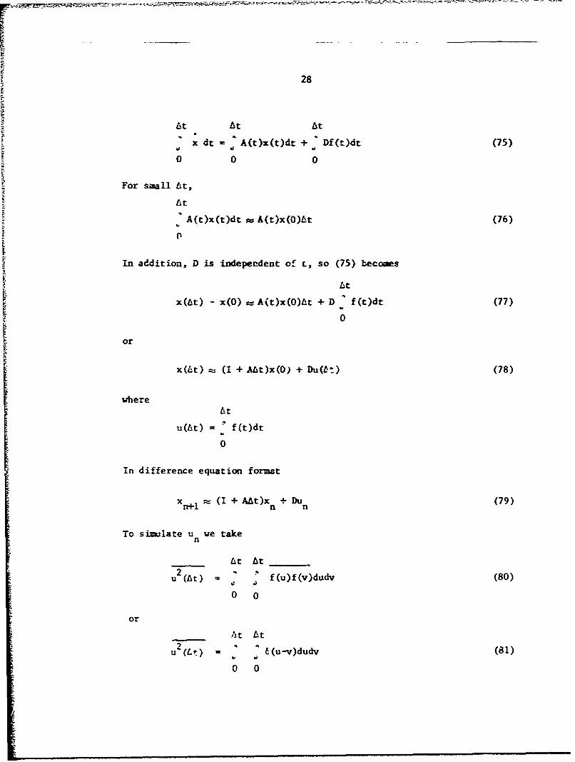
At At At

x dt A(t)x(t)dt + Df(r)dt (75)

0 0 0

For small At,

At

A(t)x(t)dt • A(t)x(0)At (76)

In addition, D is independent of L, so (75) becos

At

x(At) - x(O) =A(t)x(0)ft + D f(t)dt (77)

or

x(t) (. (I + ALt)x(0) + Du(Mt) (78)

where

At

u(ft) = f(t)dt

0

In difference equation format

x rfeIz (I + A~t)x n+ Du n(79)

To simulate u we taken

A t At

u2(At) - f(u)f(v)dudv (80)

0 0

or

At At

u (Lt) 6(u-v)dudv (81)

0 0

If 29

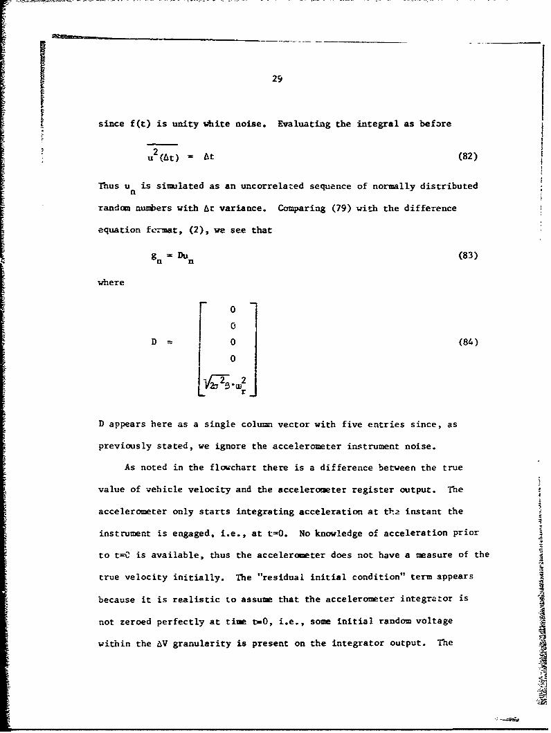
since f(t) is unity white noise. Evaluating the integral as before

u (At) At (82)

Thus u is simulated as an uncorrelated sequence of normally distributed

random numbers with At variance. Comparing (79) with the difference

equation fe.mat, (2), we see that

gn D Dn (83)

where

0

0

D 0 (84)

D appears here as a single column vector with five entries since, as

previously stated, we ignore the accelerometer instrument noise.

As noted in the flowchart there is a difference between the true

value of vehicle velocity and the accelerometer register output. The

accelerometer only starts integrating acceleration at thŽ instant the

instrument is engaged, i.e., at t=0. No knowledge of acceleration prior

to t--.. is available, thus the accelerometer does not have a measure of the

true velocity initially. The "residual initial condition" term appears

because it is realistic to assume that the accelerometer integrator is

not zeroed perfectly at time t=O, i.e., some initial random voltage

within the AV granularity is present on the integrator output. The

30

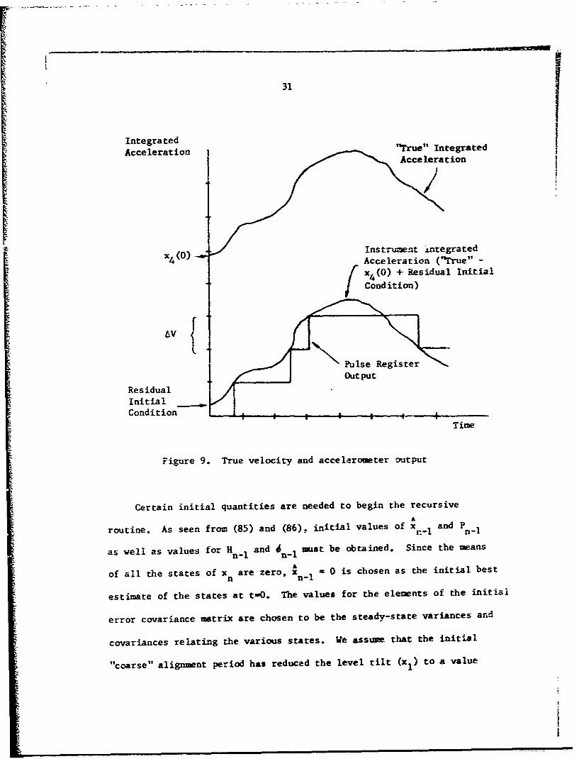
relation between these quantities for a typical velocity function is

illustrated in Figure 9. The AV quantization ,:sed for the siwailation

is taken to be the same as in :6] and is listed in Table 2.

C. Delta Velocity Kalman Estimator

The subroutine DVKAL is used to implement :he incremental velocity

Kalman estimator. The recursive equations used are slightly modified

from those given in (10) through (16). The relationships are

It A

X, = lnl - (85)

x = ++ - Hn (88)

b = P - ILI T (89)

n n n n

with the quantities as previously defined. Modification is required

because the "step-ahead" feature of the Kaluan filter is not possible,

as the time increment between neasurements is not known until the actual

measurement is made. Thus, it is not until time t that we have accessS~n

to the value tn - t . lThe a priori estimates of xn and Pn are

obtained at tn by evolving the optimm estimates at t through (85)

and (86).

31

Integrated ru"itgaeAcceleration Acrelegrateon

(0) Instrumment Integrated4 - Acceleration ("True"

x 4(0) + Residual Initial

Condition)

SPulIse Reggis ter

=-• output

Residual

InitialCondition -____.+

Time

Figure 9. True velocity and accelerometer output

Certain initial quantities are needed to begin the recursiveA

routine. As seen from (85) and (86). initial values of Xn.I and Pn-I

as well as values for Hn-i and in-1 must be obtained. Since the means

A

of all the states of x are zero, x n-1 = 0 is chosen as the initial best

estimate of the states at t-0. The values for the elements of the initial

error covariance matrix are chosen to be the steady-state variances and

covariances relating the various states. We assiue that the initial

"coarse" alignment period has reduced the level tilt (x1 ) to a value

32

Table 2. Quantities used in the simulation

DVKAL

[1 0 0 0 0

103600 0 0 0

Pn[(Initial) 0 0 8.808 0 -. 47741

0 0 .47741 01

0 0 -. 47741 0 .2184 j

Pn-l((,I) in (Uinutes of arc)2

P .1(2,2) in (minutes of arc) 2

n-1

p 1 (3,3) in (inches)2

Pn-1 (4,4) in (inches/second) 2

?n1(5,5) in (inches/second )2

V = E(iy AT) (.IAV) 2 = (.0394)2

m = (-gbt ½gQ2 t2 0 1 0)n n x n

N = (0 0 0 -1 0)n

Axn-1 =0

AV = I cm/sec = (1/2.54) in/sec

TIJAL

P* (Initial) = Same as P aboveSnni

2 2 2 2V = (V) (1/2.54)2 In2sec

n2

m =(-gt 2g.• t 0 1 0)A= x

fLt 1 I c'cond

33

having a standard deviation of one minute of arc while the azimuth

error (x2 ) is assumed to have a standard deviatiot of sixty minutes ofz2

arc. Although we assume zero initial cross-correlation between x1 and

x we must take cross-correlations of the noise states into account as

the white noise driving function distributes itself inti these states

as the process evolves. Values for these steady-state noise variances

and covariances may be obtained by choosing some arbitrary F matrix- n-i

and letting (86) evolve until the values converge. Note, however, that

as time approaches infinity 4 approaches zero, thus P (t isn-i an

equal to H (t - a). These values are readily computed via the HPHIn

subroutine (discussed in E below) and are given in Table 2. The Hn_1

and 6 n-lmatrices are obtained from the HPHI subroutine each time the

equations are used. Other quantities needed for the estimation are

Vn, Mn, and N and are included in T-ble 2. As noted in the table,

V is not 4ero as was assumed in Section III. The desire to insure an

"safe" measurement model for the simulation led to the addition of a

small amount of measurement noise. If the measurement noise is zero

we see from (15) that as P-I decreases, Q becomes very small. Since x

and x2 are deterministic, these elements of P eventually approach

zero making the value of Q subject to computer round-off error. Q can

in fact become negative, causing the Kalwn estimation to diverge. In

addition to the divergence problem, almost any physical situation has

some small amount of random noise nresent at the measurement. The

addition of the measurement noise thus makes the neasurenent u-,del

"safer" in a physical sense. The magnitude of the noise is assumed

34

to be 10% of the incremental granularity.

Since we asswm that the accelerometer integrator is not perfectly

zeroed at t-O, the first AV meacurement must be ignored as the At time

interval at the time of the measurement does not correspond to a true

velocity increment.

D. Time Interval Kalman Estimator

The TIKAL subroutine is included in Appendix A and implements (4)

through (8) to estimate the various states. The accelerometer pulse

count register is assumed to be sampled every second rb6 (i.e., At I

second), thus H and 6 are constant matrices with values obtained fromn n

the HPHI subroutine. The initial a priori estim&::e of xn is chosen to

be zero while the initial error covariance matrix, P , is obtalined as

in Part C above. These and other quantities used in the estimatton are

given in Table 2.

E. H1II Subroutine

The HPHI subroutine computes the state transition (PHI) and driven

response covariance (H) matrices in closed form, given a specified time

increment. As previously stated, PHI is obteined from the inverse

Laplace transform of (sl - A)- and in general form is

1 0 At 0 0 0

x

0 1 0 0 0

0t)= 0 0 6 (At) (90)1 33

0 0 I through

L0 0 65 5 00

35

As noted in Section III 63 3 (ft) through 05 5 (0t) are of the form (56)

where Kij., Lij and 9iJ have been previously computed and are functions

of C, f, Wr, anda .2 rI•. T

The H matrix is defined as E(g gT), the covariance matrix of then n n

state response due to the white noise input. The first two states are

completely decoupled from the white noise input, thus the corresponding

elements in the H matrix are zero. The variances and covariances relating

the final three states are obtained by forming :onvolution integrals in

the manner of (57) through (61). In general,

AC At

gig. = xx = Wj Y.(u)y.(v)6(u-v)dudv (91)

0 0

At

"iy(v)y (v)dv (92)

0

where yi(u) is the weighting function relating f(t) and x.. The various

weighting functions are obtained from Figure 6 with (92) having the

g- neral form

- 2 4[K e-2BAt• -- •g2g. r

-L (•eKw,)At [-(f+Cw) sin (-,t+) - cos (DMt*iC

13 C

I(1) t- t

-(54-tr)At [-('-tr) sin (DAt+Oj) -r ( cos ( )At+6 )+ Mij e j

SLC

t.

k3

36

+ Nij Cox eL -j -2CW r

(93)where

C + . 2 + 2C2r5 + W2

r

and

The constants Kij. Lij" Mij% NIj, Pij, and 6. are again precovmqutedand are functions of C, 9, 0, and c2

37

V. RESULTS

The performance of the incremental velocity Kalman estimator (DVKAL)

was evaluated by comprison with the "standard" time interval (TIKAL)

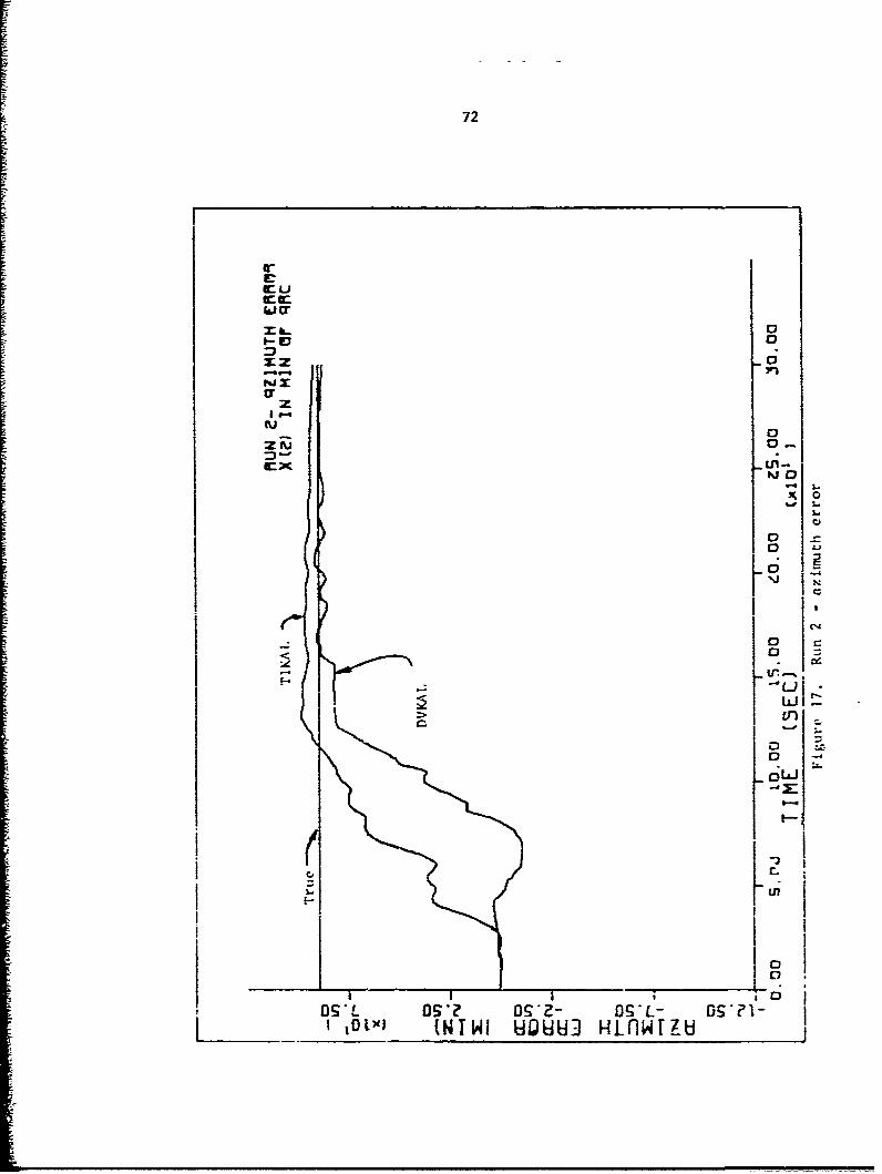
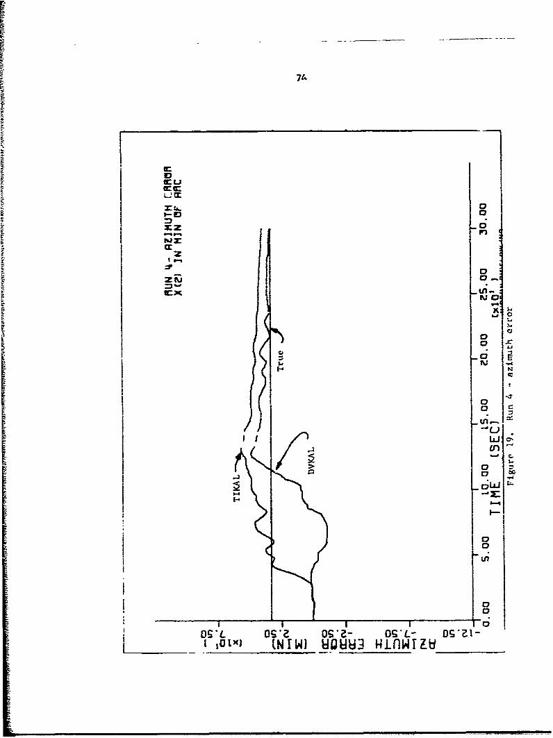
system. The results of the ten Monte Carlo simulations are shown graph-

ically in Appendix B. The DVAL and TIKAL estimates as well as the

true values of states one and two, are plotted versus time in these

graphs. In addition to the state estimates, of course, the Kalman filter

also computes the error covariance matrix. These error covariance term

for level tilt and azimuth error are averaged over the ten runs and

plotted with the actual squared error in Figures 10 through 13.

Two factors mast be considered when evaluating system performance,

these being the accuracy of state estimation and the speed at which this

accuracy is attained. Examining the azimuth error estimation curves in

Appendix B, we see that in every case the incremental velocity (DVKAL)

estimator is st perior or equal in both accuracy attained and speed of

response. Trarsients that appear In the individual runs are due to system

dynamics. The t.stimates and trt'.- values for the azimuth e:-ror at the end

of the alignment period (300 seconds) as well as the RVUS estimate errors

are given in Table 3. If we define the acceptable "criterion-of-goodness"

as estimating the azimuth error to within five .zinutes of arc, we see

that adequate performance is attained on only three -if the TIKAL runs.

This also is illustrated by the RMS error tera- which is greater than the

required bound. In comparing the response times, we observe from

Figures 12 and 13 that the average square of the DVKAL azimuth estimation

error is within the desired bound (25 mn 2) after approximately 200 seconds

38

*0Lhi

0

Cc- 00-

-in

0

0 0.

N0

0* C

0 0:

00

0

00*1~~,- SU -DGZo0*

(?.NIWIuiC *Ztns O U

39

0

w0

0

w~ci

ki

m 0

oo

00LnI

> 0

o 0

SU 2* 00

(EN IW) 03tinosUDUU

40

etcJ

kJM

0.- n.

m -6-

"~~ 1facJ

0 W-100

wJ oo0

0

oLA

C.'i

in ,.

00'h 00 0, 2 o"I o oI to1XI 2N IW) 03"utnns QU0

4 41

cic

cy 0

""Jo

bit

-i

w0

cc

0

0

0 ;6

0

0

1-.

cn

~50

00'h Dot~ 00,2 0 1 00,0~O~') NIWJ OJutffnJs UOQUU3

42

Table 3. Azimuth. error (minutes of arc) after 300 seconds

Run True Value DVMAL Estimate TIKAL Estimte

1 47.208 45.239 57.320

2 89.544 87.214 91.554

3 -5.046 -5.262 -8.219

4 33.240 32.650 39.217

5 -47.490 -47.280 -54.528

6 -81.720 -82.121 -83.994

7 13.332 12.240 4.174

8 42.780 40.228 33.007

9 58.116 54.924 64.869

10 -106.248 -104.198 -112.373

RMS Error 1.789 6.856

while the TIKAL error never reaches an acceptabie level.

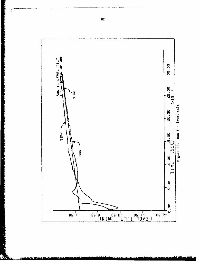
Results for the level tilts aze similar except that the estimate

is obtained more rapidly. The reason for this is that the only measure

that the Kalman filter has of azinuch error is its connection to the slope

of the level tilt. Thus we expect that th- filter must first estimate

the tilt correctly before it is able to accurately estimate the azimuth

error (which is constant).

The above results are not surprising as the TIKAL measurement algorithm,

in effect, models the physical situstion incorrectly. The signal phymrically

available to the TIKAL estimator is a measure of the total integrated

43

acceleraticz. from the acceleroeter (Figure 8) and is dependent upon

x 4 (t) and x4 (O). Since the estimator has no a priori knowledge of x

its best estimate of x4 (0) is zero. Thus we suspect that as x4 (0)

becomes larger the performance suffers accordingly. The DVKAL scheme

is not affected by this problem as it uses an incremental measurement

and estimates the necessary present and delayed states.

Another source of error is the "residual initial condition" which

is the randoui initial voltage on the accelerometer integrator. We see

from Figure 9 that the resulting integrated acceleration function is not

zero initially as is assumed in the TMKAL estimator. Since the DVKAL

technique ignores the first AV meaaurement, errors due to this residual

quantity are also avoided.

The random values used for x4 (O) and the "residual initial condition"

as well as the final squared difference between the azimuth error true

and estimated values are listed in Table 4. The actual numbers listed

for x 4(0) and the "residual initial condition" are unity variance random

numbers with the necessary additional scaling shown at the top of the table

(the "residual initial condition" does not have a truly normal distribu-

tion as it is not allowed to exceed toe granularity AV). As seen from

Table 4 there is a strong correlation between large final errors in the

TIKAL estimation and high initial values of x4, thus verifying our

previous suspicions. This effect is illustrated by taking simulation

Run I (which had a large value for x (0) ) and setting x4 (0) 0. The

result is shown in Figure 14. By comparing Figure 14 with the corre-

sponding graph in Appendix B, the dramatic improvement in performance

m44

6L-

10020

z

W0

U,

0xn

09* 0G2 o~- O'L ,?I

lotx (WII WUU3 inw zf

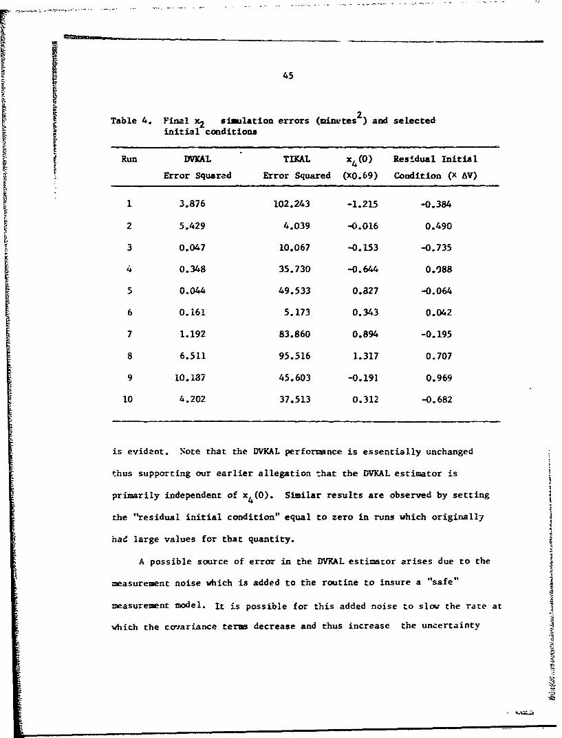
45

Table 4. Final simulation errors (minutes ) and selectedinitial conditions

Run MVKAL TIKAL x4 (0) Residual Initial

Error Squared Error Squared (XO.69) Condition (x AV)

1 3.876 102.243 -1.215 -0.384

2 5.429 4.039 -0.016 0.490

3 0.047 10.067 -0.153 -0.735

4 0.348 35.730 -0.644 0.988

5 0.044 49.533 0.827 -0.064

6 0.161 5.173 0.343 0.042

7 1.192 83.860 0.894 -0.195

8 6.511 95.516 1.317 0.707

9 10.187 45.603 -0.191 0.969

10 4.202 37.513 0.312 -0.682

is evident. Note that the DVKAL performance is essentially unchanged

thus supporting our earlier allegation that the DVKAL estimator is

primarily independent of x4 (O). Similar results are observed by setting

the "residual initial condition" equal to zero in runs which originally

had large values for that quantity.

A possible source of error in the DVKAL estimator arises due to the

measurement noise which is added to the routine to insure a "safe"

measurement model. It is possible for this added noise to slow the rate at

which the co-zariance terms decrease and thus increase the uncertainty

g• • • • am m • • • me m m • • m ima •4,

46

associated with the state estimates. In (15j and (10), the added noise

decreases the gain, b , thereby weighting the measurement term less.

Improvement in MEAL performance for Run 9 is illustrated in Figure 15

by setting the measurement noise equal to zero. The DMKAL response with

noise equal to 10% of AV is included for comparison. Thus, at least

for one run, improved performance does result from decreased measurement

noise. This means that a smaller value of measurement noise should have

been chosen for the simulation. A study was not conducted to determine

optimum magnitudes for this noise and the value selected was done so on

a purely heuristic basis.

From Figures 12 and 13 it is observed that the TIKAL covariance

quantities approach zero faster than the corresponding DVKAL values.

This is primarily due to the aforementioned DVKAL measurement noise and

(for the process selected, at least) a larger number of TIKAL measurements.

1~we 0

Ojz01

- I-

IV0

Co

'U

1009* 0sz OSL 0521I toEX N W -U3 iwiz

48

VI. CONCIXCSIONS

Under the conditions and limitations assumed (e.g., zero accelerom-

eter biases), the incremental vel,:ity (DVKAL) measurement algorithr.

is superior to the time interval (TIXAL) sampling scheme in both accuracy

of estimation and speed of response. Although the results presented have

been obtained using a single physical process, the positive nature of

these results indicates the need for a more extensive study to further

establish the performance level and limitations associated with the

incremental velocity technique.

The errors incurred by the time interval Ilgarithm are derived

primarily from its improper modeling of the physical situarion.

C 49

"VII. LITERATURE CITED

[11 G.R. Pitman Jr., Ed., Inertial Guidance. New York: Wiley,

1962.

r,21 R. G. Brown, "Kalman filter notes,'* Dept. Elec. Egr., IowaState University, June 1968.

L3 j R. G. Brcon and G. L. Hartman, "Kalman filter with delayedstates as observ.a1les,11 Proc. National Electronics Cnf.,July 1968.

[4] T. B. Cline, "Suboptiimization of a Kalman filter with delayeastates as observables," M.S. Thesis, Library, Iowa StateUniversity, 1970.

[5] R. C. Brown and J. W. Nilsson, Introduction to Linear SytemsAnalysis. New York: Wiley, 1962.

L6] L. D. Brock and G. T. Schmidt, "Statistical estimation ininertial navigation systems," Journal of Spacecraft andRockets, vol. 5, no. 2, February 1968, pp. 150-153.

"L7 H. W. Sorenson, "Kalman filtering techniques," in Advancesin Control Systems, vol. 3, C. T. Leondes, Ed. New York:Academic, 1966, pp. 219-292.

i4

50

VIII. ACKNOWLEDGMENTS

The author is indebted to Dr. R. G. Brown for suggesting the topic

for this study and for the guidance given during its investigation.

This work was supported by the Engineering Research Institute through

funds provided by the Office of Naval Research, contract number N00014-

68A-0162.

51

IX. APPENDIX A: SIIIJATION PROGRAM

A. Main Program

= _ _

52

0-

Z ~ U I--- I

Wu Wj LIE z z

9- U- M

3:I -c- <

+ > 10.-

U. z I.- D 4c

X 0M I- W W1

0.0- -I- w u.J

* C; o0 i- U. >- 1 Ww w -~4n I. Z0-- L I

W - - W0 X 1 u i Li""<o ZifI- 4 . w 0 0)-*OWZ 0 II-t

I 4x~Z 0 w .4 1-4 . 4 " 4 4cuu0 Z .- 4Z 44 U a u- a-

-a 0o _. S.- 4: 40 a O0. a6-a- -a um--j c

0. 0 ujl-Z . Nuuz q U

ZLu ) a )0 c --4 Li ~ > U.o 0

'-0o. OuZOV)~n qýwZ l- P- in 0,4Z W-XO--WZ wco..ua -P..Z _J C:w

ifli 00-w ZZWi. c W) w AZ OZ"C..: -- u->I- .- O- at > *-

Li ZVW & -U -' W~

0 Li "m fi C) D0 -I4U'- ý- * Z-<Z - oC o0pC )0-00W - W AZ W- -*L ýlý0 UI Z 4a U.. )-D -. S- p-

o0wi u.~ - z0 CD >- W -a- a0 .- 0 44 ' I.-= oLJ >-I

Z~JI Z)4nwnx0 a Z- Z)V 0 .-

53

NO

x z*

u.. WI

Z 0ZU. WLL

uiUZ.-W

x4 Z. z .- z:

Z- oEU Z

z Lu

In 0w 0 w 2%7 of ft-.- _j 8

c-U UJ 4 b..- uwO

Z -0 0 ccU ZD 0*V uc4 - 3C 0w 0 x 0

zx I. *. -4-zI.- -CLu 0N ct0 D 0 v -

oi W - w 5* *- 0 n 't V 4 *LU. or- LLOI- * 0+ .* c

8 ~ * -c NW Lu InC'o

*Z 0* cc ~ U- a)..J 0 0

< 0- n 6 cia- 0 -4 <mx" W4. l- @-ai _jU i * c- W*IA.A J 9* 7-C. %n .On9 -l

In - L) m. LiUn us 0- <- -W -X 4. - Uin~~ .0 0- -K--- 1-ZwW)V4-0UJ- &f&.-U WK OJ u.4b0svW a*Uls

4UV c) .C.N -4 X.0 J . X4)ft )( 3L- - - 4Aa .- V)Z- t, 0 0- *b**.)CU *44-w - e

Z 4A -u. LA -4 -N0 0- 01 C X

"o - 0 I 4N9 U .'0--Z - a a -a- -L -C S.-w Box got-$.- OulZ Z.a i-'. O -ic'

09 Z Luin cr a-e4 K v)l' a 9i- X -CC -- u--

- a WISL 0.4. -1 0.- <U iK. a%. a

00 0. (nwot zw Lu U l-j I 0K . ww cr .

00 C C W O-.j'0- 3 S

54

a, -O 4 4, -C:-.t0 0-0 V4 0) i

01 &1 00. e-4 -- 4* + + * %t

< LL

0

W X C ( .* w I i- I.- 2

0( ~ X JA~C M Ln- %"uý , zUt*- lo Pt 0. P- 004, a c4iinI - 0ngat~cJ-ýr z,. > -9 Lu x 0 .

4*J*.4.0Lu Z Z wLL+ 0 0--j10

LU z z 9.9

- 0X

wX Q~s x * w wZ I--r 0 0 mu- 0.le Zl Z --xOD~*u*j W p %t' ent C0 0i 0i P. 4 X

mit. w0* 0* -, .41 00 49 U1) 4j xU Xi4. #

4 to J4.-S , %m - 0. 4- 4n x D~ZOD 04 '..J OD zY b- CD0 -o-U . CU -

* * .eu.GN4c )CUNOOXC4- - JO .- + Z4'- 1 CO0OV)% '.j4D* )C.j Z Z 49o-o 0 1.-&L1L44.9N 3s 1 . *- * W * -4 X*4K 9.- l 9X.1- m 0 3O LV

ul UN x - < a a 8 5 V) I-e- 0 B - -L~. .. * ~4 .* - - - -j V -oxv ~ i.,.tmu-z o

Cl CL

0 e li Li %-) oo- * C.) rvCV uJ1-

55

z

u-j

LuLA.

LuJI- CL U'

If . Ci W

+ -j M4 C1 V

U. N : W (V

* .j M LL -j

U'~§A IV) Ca.

-~~ C., * .'I)

4 1- 2: 4D-~ ~ ~ U Luxa- - u UU' C.) x z I.--2

W InJ LuJ 0.-4 ai uiA -i Z 7y

9.- V: fl- Cl C, LI u. 49l uj el-j V ) W ta Or w "

Ua 0 - nU.

-4 0. %A L, ISI .

C i 2: Z4 C)3LA, .-j +. Lu > I.- o") V. LO

x 1 42 f- uj em a) Lu9j x 0n - a) vi 49 x i

a,- 3. C) w0 Di 2: I0 L;LLI.- x 1 CL .J 3E7 L 3: Lu a-q ) ..-CL 4 CIn f ' > > > -

CL %T* C.- 40 -A w -w- I-- -j ib-U0&-XCI9-V0W4 w3 j :4 a. - X9- '0 V.0

il U..,. 4 - 0 0 i-i-- +- CGO ) &L L. 1 I-- 0 an C.-i- alu - 0 > , C-- Nj w w-C >

> 4,ý. _ja0 .. 't -d '0 4ý )(3i C

LL 4-) -j : w ca. 0>> .. W 0>> w

>~.. g> -) C)- C),CUC~C

56

N a

LU Lu b.

0W WO .- -. - -<w tAnZ -Ci-- X elLA- .4 )X uW

-j CC,~ 0 w uV,

cuan = - a x cyin=

ai -7 .4 -7 -C

*X C ~ wýXv Ci c.ufn C" (1)f X en W .

2z XI .11 -. 0; fXfl

*w w 0 ev x 01Oi *: C4 N.

w . ' U- '- or wOr enN CC. X - -.

tv i.- x We N Cm .0x

- a 's 0 -X - -40. -. .1- I-. - DX -I*-' IU..- 4

I X X u4: x g-X4i =en V4 C) w tCu-4 cn C:

w I 2: 0 aI U% w ~ OD

Cca 44 eX w 3 aXa CC 4 4- N~jx

WiXu 0 ILI ui N e) I,- oujLUJ a .*CCMw wL U.X .x m U).ZX ~ X-QDUJ

-ax x P- < - I- I.- w . U...W *)(-4 0I . 1--I-- w x' 0 Z x 3ri Nb> u'~ -a~~.J UU xJ xW % O ~ a ~ .. ~.. D.LU -Xt u LU.- 17 0 6. *a -- X -Ui 4LU..O u .

w . .j4 LU .i (A I-- W% -.- -o 1ý- ) 4- cwz 4.. Oe X: 00I. - X-Z 0.0. W fn COI M3 - x.4 D w Z n- Z- Z tr

C)- CV 0 .- a' 149 ui ' ~ 0 1- ccw NoQ 0.)*aw A. CC 44 ea 41 - cc% -a' CC V- . -U. IlOa. U., - . I-- X .J. > -- X -inV4 pc- U.. 0 .

on fn a- IA .- I-4O< a -'L w N ee- UN fn.- '-OW3. ,a - X.~ Zx> + -x , r-- - X I-aX D(4IIA C. -I- OD M ~ a -Ji IZ W I.-w in. O ff. - A--= - I.- z

0- OXXL0owI-74 *CS-O..aI cnal---j=4. -7, *XI w <L4,..---Iac U. -m WU. *4. Ir a 3c -9 z ZCC CC e- fn~ rIfUL CC w Z

i.- w 39L I-- 3eLi0-41.X u- -L3t wv- '00n4 n .0 up (Ar 4 0~ v- v n-Z&

IA Dole x IA crin.- C

57I

44

100

i.-1

e.-aZ

* * J uwZ

z'n-D

='

58

B. DVKAL Subroutine

59

0.-

S*- sfoASO, Z

0 0

'I-

Sn cn a-

0 w U-.

x 0- W).

IW I.-r

- .-IIf Lu0I- o--in- z >

.0 0 C

.0) .-- x 0 U.0C) Z -- :)

.J Q in - 4d2

qIx -O J1l WOO -. . uj )e % t

Oj> .-4 an. In o .- c

a U) U 0 L1

X- 0 N ii%

Lu>Au *In Xvm it ica

wli U'1-O- ~ -JW 0 ji nV

40>0<X W"ý -ZZ 019 mO CC-- - ' - -- ~ -*uSZuix L.'O4I

CA -0 w -~ cc - - -

Iý .-4 .tu1 orw r I- > I--

CI

I-ap.- ~3E

- ~ frh -tLJ U.Cie

LI,)

o4 X

%n CL~ 4a+

ý* V4..- -ILN I- x - - " ' -. t 04

Z I ( 1 91 * * i n w

*~~ Z,- Z~ ; -

CL a

ND *4 4z * * X

~~.*Z 0 IN.

W

2 a4 r'-0-~~~ ~q a

~ -W . :r Q ~ 40.4~U

4 q-M~..4 't

.**O..*~~~~C9 * IZ - C a -, '-

Z ~~- C> N C. - . a v E %N~1 WW-

N 0.Z 'OZ

. J I" 4x + . . '.

1..X ) U CL OF is

61

a x

II

0 x

0 #. , - .

01

a-301 30. u

0- ZNwx w

U- Vý 0 i

UN C:) 0.&-

Ow 4.4 0..P4

Z ~ ~~~~ I I x2m Xaa

0 ~~' CLD 1 x-

V4 G 2u0.P- 0o ui c-

0- 0 * -a co-t .~ 4( a -WIfY ~.

62

C. TIKAL Subroutine

I

II

63 _ _ _ _ _

xI

UN'

4n in'

4 . 44.4

< -.

b: X: 4% 0JI-.

Z - PA^ u 4 L .0 0

T -.- &n 0Z W WO

-J12 I-Zu W Z n

1- 441 4n P4 0ti %4, KO. z- *CD t 4 - .C

N e1 C) X % 0 d 0P-wm 4- X <

X0V c. UN ZZt> nin4w

D-W 40X -0a- c- Un 1O

.- a: cc I... a I-m a a=Uý 4,c qI--4 M( q.. V%- * n nM --

M1 Z U LU - >0 Z w -Ic Q ~ 0 .4,U

4n L I U .-Lrav'd) 4 wwZ .)%

~J'4Z .Z W U t- eelCL 41Q .~6

u.Q..au s. UZ *0 4 t 4

64

.>

4.

x -41

a- .! &i a-,

re Z to

0L 1 1 cm

.41 Wt 0

tv Ca I

-z - W* -a.

*r - -Va &''

m I.- cucr X CL- wL

< w- Q-iLL a~Z P- - X- Q. CL a: a.a

m mW U)-Q 0..-+x v* +'.- 4* t-0 0 --- + -

z 1 I0- - * U*a W-. s-iaC.vCL. Uj.V4 X3- 0a. $-.. *-a a a W31- W u .- u -. x 't W

- 0. 0. 0. CL .4 a. w -4&Oi 1 ~-- O'Ww 0 0- 4W

.4~e .4. 94-4 4%6-LI 01 OD LI Lu zI -r

1 65

In CLiI;J

eZ4- D zJ

z a. z0 -ooxdbh-noz

M -- 0-

66

D. HRPI Subroutine

67

X- *

* 4z

Wo -f i

.4 Co*- IW 0

1-4- 39* *n

-~C j* -t* -%._ Y

U.O o.a UN0 %v A60v4*4 ZCit ~-z ie n4 - n w

Z4 -- vff40 - 4tt- W - Iw -

I 0 *U0 -. Y L _ n3 e - . a4

a e- N8 t

CO -j ft a of- 001- at --

ft . Il'A v &y30 A .u* 4 W

68

I.-

4. IL 4zN~w*4.cm

* w 0-

In) + + *z

X * X*;;* *

CY CY Wa~

39- u

* * I* I U*4 0

- 4 U* *II- Iq u N0zCMi 0 - 0* tv* *U 9-4.

* t m W -- C .% mC * W m *Uj -4 * .. 00

cn0 .* .*- N%. "...N * * * D0O%** 't. e. or N39 Z f0O 0* %.) v" CD 90 9, .4 ** 1 0 XdD X- 39 P e i P-a* -L'I ID X I I I~ &C I CDD-5 I8II - 3CI # ICm'.:Ww qA

a5 a a a- a a a a - a a a a 0 a a a &.- ". no I f +*

N X 0.-iCD 10V

C~j fr.+ #-I#.)

69

m~ 0-0 4 4 4

'O .04 * U, .0

o0 1 .- L)*IU u

* - 0.. Z Z Z

Z * I) I4 a aU *V. a - .- a I

1i- * 3u *L W*1W Awl xi wui

WO.-O* en4**0i0 e lX ~ J W% cu I

t- V4 P- m ' t U' 0

CV 9-~4* 00.

*c C I - I-lI

&,I X M Ux & &OCC UJ-X X*w*WLL&j

x I.- UN C -t u0%4. 4

w waWaago

:) 0-- - -t) - (flM 8 wm -0*Z U UNE I I .In0+( z - ZA 3- - .- V4 eaa en a' *t w w Z

MIEa, U I IIJ f .aXU. aS.'. 9.. Z c UU ZZ*. t wWI

04 ue 0 II I. Q C.d V" C.C.C CC,

L; u 4

70

X. APPENDIX B: GRAPHICAL REtUrLTS

A. Azimuth Error

71

Zk.0

cr0

0n

- iI 0

-- 1 0

to~~ ~ ~ ~ IX NWIUU3 o i

72

X6-v 0

x~z 0

I.-q

(uz 0

0oj

0l

u,

_JLL,

j I lI x INIWI UJQUUJ HLOwTi3~ ~~

73

CC

z a0Zk.In

U~q gq

OwlO

t.

OS' Los~z os~e DS*- KsI lot) (NI W)UQWU3Hinw5.it

7A

ICUW- m

Li M51z

x z 0

N. 0

I C31

0 a:

I- ~iv -n

'-4 0L&' Z- 0 * - D~ l

I 0OX(NTW) OUU3 inwUa

75

IccLim

CC00

rz_0Fn

I,.

zn 3w 0-

Ac0 0 3

0 £0

C~u

0

S, L991Z 09,- 09L- 0*Z oI to x) i~wi U UO H'W[Lb

76

ccum

CLz"&"lux:

0z~u 0.C)( In

os i. OS' os~z nclotx)~~~~m (NNPQU %h [t

77

0

zz 0

0

r,., L0i

to -(I (N~ 6U3H1w

78

cu

xzL

I" I .lk 0

104

- s Isz &L- 0 '

Dix) (Nfl YOU3 ~nw zo

79

IFo

I&JZJ

hi.

'Jo

0'

f0OG*LGG'2 05'- OSL- 0 'a 0

I JOIX MIN)69HU3 inwiz

80

LimZ

t z

0

in-

C),~

lol1-

0

OS'L~ We.~z )SL '-l

I loi) (NTWJ QWU3 Hinwr zb

81

B. Level Tilt

82

I- C

k-L

00

-i

z I~

E-4I

00-. 4

0~~~ s 1 t'D SltNTWI ~ ~ LI -33

83

0

-4J

z.-4

-4

>

oL2

0

6be

E- 4

(NIW)-4I 3 3

84

IAJwitk 0

kZ

00

0

r2t-4

C-n

00

OS'l s - Dosn-INTW)L~lLý3A3

85

iLI

9-, 0

Zipg, 0"P

LJZu 0

LiJ

-tI

0

if;u...

j Ca

-U7

0*09 * 09*- Dsl- O' ?I

(N r ) Llr 13A0

86

s-C

-0

V 0

bIZ

-jA20

Inn

CC.

DUI

-T--

09 1091 OG*- 0 *1- 9* oiwrw Lir13Ao

87

0

Z:: 0-

VI 0

2C

5.-rSnf sl- sos?(NIW Iw 33

88

-j c

uzI-j

IV0

Zr.i

'-,4

I IALD.

0&11 s~o -qlo- os*1i NI wi l L133

89

L4i

000 :

Li 4-JL

too

6LLJ

OS'D oso- os.z

IN. -I I L 3 3

90

Iu0

vz 0

-j

010

in

K41

-4

o40

-0 >

0

00

14 dwl

U?

o~to

(N IW) 1l1i 13A31

r 91

_rc

fr-L 0

bV z

00

COX tn-w 0

4-4

4.1

0-

C2in

C2,c

0 -4

0

0

O-O-(Nrw £111O I 1A31