february 21, 2000robotics 1 copyright martin p. aalund, ph.d. computational considerations

February 21, 2000 Robotics 1 Copyright Martin P. Aalund, Ph.D.

Computational Considerations

DOF4 6 7 10

Algorythm Adds Mults Adds Mults Adds Mults Adds MultsK 36.0 36.0 54.0 54.0 63.0 63.0 90.0 90.0IK 411.2 1372.8 1915.2 4230.0PC PID 21.0 16.0 31.0 24.0 36.0 28.0 51.0 40.0PC PIDG 169.0 186.0 263.0 286.0 310.0 336.0 451.0 486.0PC STR 727.0 838.0 1141.0 1294.0 1348.0 1522.0 1969.0 2206.0State Space 156.0 168.0 234.0 252.0 273.0 294.0 390.0 420.0Torque 516.0 482.0 824.0 760.0 978.0 899.0 1440.0 1316.0D 1364.0 4448.1 7161.1 22660.3DC 16912.0 32610.0 43170.3 90070.0


Kinematics

• Kinematics can play a large role in both the computational requirements for the robot, and in its range of motion.

• Most industrial robots have simple kinematics to reduce computational burden

• Often have spherical wrists.

• Almost always have 3 intersecting axes.– Pieper’s Solution guarantees a closed form inverse

• Sine and Cosine terms handled in look-up table.– We can store both the sine and cosine in one table.

– Need only one forth of the full table.

– A 16 bit look-up table would require only 32 Kbytes of memory.


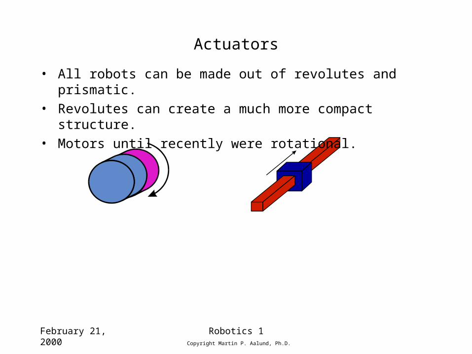
Actuators

• All robots can be made out of revolutes and prismatic.

• Revolutes can create a much more compact structure.

• Motors until recently were rotational.


Workspace

• Very dependent on the design of the manipulator.

• Small wrist Sphere or circle is important– Use Gimbals

– Combine actuators

– Reduce length of actuators.

• Reach of robot with a spherical wrist where all angles are possible is:– Distance to wrist minus the radius of wrist Sphere


Workspace Example


Wrist radius Vs workspace.

Actual Workspace


Arcmate Robot


Shilling Arm


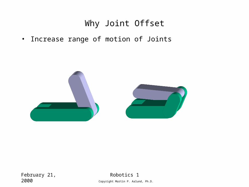
Why Joint Offset

5

• Increase range of motion of Joints


3D Parallel Mechanism


What's Next

• We now can calculate the position of the robot based on the joint angles and the joint angles based on the end-effector position.

• This is enough for very simple motion, but if we want to control the speed we need more.


Velocity

• Velocity is the derivative of position with respect to time.– Linear V

– Angular • Velocity vector is associated with a point in space.

• Velocities are relative to reference frames.– Train, Car, Fixed

• Speed is the magnitude of the velocity without direction information.

• Velocity contains information on direction and magnitude.


Example

Y

X

YX

QA B


Reference Frame Velocity

• We need to know what frame the position is in, and what frame we are taking the derivative relative.

• May be zero relative to some frames.– Link Example

• Frame of reference is designated by a leading superscript.– Example we have a position vector in reference frame

– We want the resultant derivative expressed in Frame A

Qdt

dV B

A

QBA )(

Reference Frame of Velocity Position Vector Being

Differentiated

Reference Frame of Position Vector

Reference Frame of Derivative

QB


Reference Frames Velocity

• If A and B are the same we drop the outer superscript

• We can always remove the outer superscript by including the rotation matrix.

• We will often consider the velocity of the origin of a frame {C} relative to an understood universal reference {U}

• Or expressed in Frame {A} but still differentiated in {U}

Qdt

dV B

B

QB

QBA

BQBA VRV )(

CORGU

Q Vv

CORGUA

UQA VRv


Angular Velocity

• Describes the motion of a frame or a body in space. • Definition

• The direction of AB represents the instantaneous axes of rotation of frame {B} relative to frame {A}.

• The magnitude represents the angular speed of rotation.

CU

C

Angular Velocity of Frame C relative to Global Coordinate Frame

Angular Velocity of Frame

Frame being measured

Frame measured Relative


Linear and Rotational Frames in Rigid Bodies


Motion of Rigid Bodies

• First attach a reference frame to each body

• Now we can study the motion of each frame relative to the next.

• The is the same methodology we used to study the forward position of the manipulator.

• Lets look at frame {A} and {B}

{A}

{B}

BQ


Rigid Bodies Cont.

• Lets look at a vector Q fixed in frame {B} BQ

• We want to describe the motion of this vector relative to frame A

• For now lets assume {A} is fixed.

• {B} is located relative to{A} by a position vector APBORG and a rotation matrices

{A}

{B}

BQ

APBORG

RAB


Rigid Bodies Linear Motion

• Three things can be in motion or changing with respect to time– The vector APBORG can be changing

– The vector BQ can be changing

– The orientation of {B} with respect to {A} may be changing.

• First lets look at linear motion, so assume is not changing.

• So we need only represent both velocity components in terms of {A}

• Remember the velocity of Q is just a vector so we can use a standard rotation matrices to transform its value from one frame to another.

• If we know Q(t) and APBORG(t) we can differentiate and plug into the above equation.

RAB

QBA

BBORGA

QA VRVV


Rigid Bodies Rotational Motion

• Now lets assume that Q is constant and fixed in B. BVQ=0

• Even though Q has no velocity relative to B it is clear it can still have motion relative to A

• The the motion is due to two components– The vector APBORG changing

– The orientation of {B} with respect to {A} changing in time AB.

– Lets look first at the change due to rotation

{A}{B}

BQAB


Rigid Bodies Rotational Motion Cont.

• Lets look at a small Q a small time later t

{A}{B}

BQ(t)AB

{B’}

BQ(t+t)

Q


Rigid Bodies Rotational Motion Cont.

• The change in Q for a very small motion is just the radius times the change in the angle.• Radius is Q sin()• Remember Q is not changing in time• So Q is just Q sin()t• This is just the cross product of

Q and

If Q Changes with Timethen

or in terms of {B} and R

Q(t)AB

Q(t+t)

Q

QV AB

AQ

A

)( QBAA

BA

QA VQV

QBA

BBA

BBA

QA VRQRV


Simultaneous Linear and Rotational Motion

• Linear

• Rotational

• BothQ

BAB

BABB

AQ

A VRQRV

QBA

BBORGA

QA VRVV

QBA

BBA

BBA

BORGA

QA VRQRVV


Propagation Link to Link Rotational

• So now that we can calculate the velocity of one body or reference frame relative to the other how do we apply this to a robot?

• A robot is a chain of bodies represented by links that can rotate or translate relative to each other.

• We already know how to assign a reference frame to each link.

• The velocity of link i+1 is the velocity of link i, plus the velocity component added at joint i+1.

• Angular velocities can be added if they are represented in the same frame.

• Remember we have defined all joint motion to be around or along Z.

11

1i11ˆθωω

iii

iii

ii ZR

1i

1

11

1i

θ

0

0

θ

i

ii Z


Propagation Link to Link Rotational

• For Linear velocity we get

• This is the same as we previously derived with iPi+1 a constant.• If we want the velocity and angular velocity in terms of i+1 we simply

pre-multiply by the rotation matrix.

• Remember that the derivatives are still taken relative to a universal frame. So vi is the velocity of the origin of link frame{i} and i is the angular velocity of link frame {i}. They can be expressed in any frame even frame {i}.

111 ω

ii

ii

ii

ii Pvv

111

11 ω

ii

ii

iii

iii PvRv

11

1i1

11

1i11

11 ˆθωˆθωω

ii

iiii

iiii

iiii

i ZRZRR


Propagation for Translational Joints

• Similarly for the case of a Translational joint we get

• No additional angular velocity component since it’s a transnational joint. Just a change of reference frame.

• But must add contribution due to linear motion of joint along Z axes

iiii

i R ωω 11

1

11

1111

11 ˆω

ii

iii

ii

iii

iii ZdPvRv


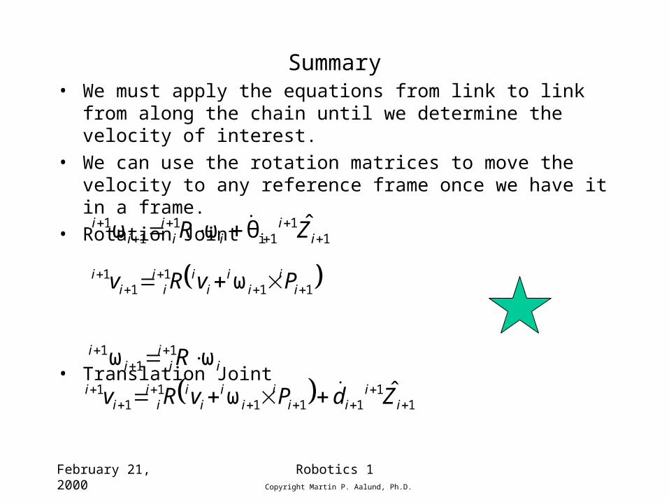
Summary• We must apply the equations from link to link from along the chain

until we determine the velocity of interest.

• We can use the rotation matrices to move the velocity to any reference frame once we have it in a frame.

• Rotation Joint

• Translation Joint

iiii

i R ωω 11

1

11

1111

11 ˆω

ii

iii

ii

iii

iii ZdPvRv

111

11 ω

ii

ii

iii

iii PvRv

11

1i1

11 ˆθωω

ii

iiii

i ZR


Jacobian

• What is a Jacobian

• Lets say we have a functions x=F(1,2) and y= G(1,2)

• We want to find the velocity vx and vy

• We use the chain rule to take the derivative

• Or in matrix format

t

G

t

G

t

G

t

yy

t

F

t

F

tt

xx

2

2

1

1

21

2

2

1

1

21

θ

θ

θ

θ

)θ,θ(

θ

θ

θ

θ

)θ,θF(

2

1

2

1

21

21

θ

θ

θ

θ

θθ

θθ

JGG

FF

y

x


Jacobian Cont.

• The Jacobian is multi-dimensional form of the derivative

• At any instant the Jacobian is linear transformation.

• The Jacobian will vary as a function of time.

• Most common Jacobian deals with joint velocities.– It relates the Cartesian coordinates of the tip of the robot arm to the joint

velocities or the derivatives of joint variables.

• The number of rows corresponds to the number of joints

• The number of columns corresponds to the number of Cartesian coordinates.

• The most general form is a 6x6 matrix. Does not have to be square.

• The Jacobian can be calculated for any orthogonal set of variables.– X,Y

– R,


Jacobian Cont

• For low degree of freedom robots the Jacobian can be found by directly differentiating the equations of motion

• This works for linear velocities but does not work for angular velocities.

• Changing frame of reference of a Jacobian.

• The general 6x6 Jacobian maps both the angular velocity vector and the linear velocity. If we view these two 3x1 vectors as one 6x1 vector we can see how we should change the Jacobian’s reference frame.

zv

yv

xv

v

zAy

Ax

A

A

ˆ

ˆ

ˆ

z

y

x

zA

yA

xA

A

ˆω

ˆω

ˆω

ω


Jacobian Cont

• We can use the following equation to convert from frame {B} to {A}

• Since the Jacobian performs a similar mapping.

• If the Jacobian is non singular we can invert it to find the joint rates in terms of the Cartesian coordinates.

• What does a singular Jacobian mean.– In general it means that no instantaneous motion along one of the

Cartesian coordinates is possible.

ω0

0

ω B

B

AB

AB

A

A v

R

Rv

J

R

RJ B

AB

ABA

0

0


Jacobian Cont.

• We can use the Jacobian to predict where these singularities occur

• If we don’t check for singularities, we can end up commanding our joints to move at high velocities.

• At the actual singularity we would require infinite motion from the joint.

• Two common singularities occur– One is when two joints line up.

– The second occurs at the edge of the workspace.

• Additional singularities may exist that are not predicted by the Jacobian.

• Structures can be designed to be singularity free from a Jacobian point of view.


Jacobian Example page 1• Given the simple manipulator below find the Jacobian referenced to

frame 4. Frame 4 is at the tip of the arm with the same orientation as frame 3

• The manipulator can be described by the transformation matrices (see Example 3.3).

1000

0 222323

212111231231

212111231231

03 SLCS

CSLSLCSSSC

CCLCLSSCCC

T

1000

0100

0010

001 3

34

L

T

TTT 34

03

04


Jacobian Example page 2

• We are mapping from Cartesian to joint space

• All Joints are revolutes so we can use

1

1

1

θ

θ

θ

J

Z

Y

X

11

11 ω

ii

ii

iii

iii PvRv

11

1i1

11 ˆθωω

ii

iii

iii ZR

IR

cs

sc

R

cs

sc

R

43

33

3332

22

2221

100

0

0

010

0

0

100

01

011

110 cs

sc

R


Jacobian Example page 3

• Propagating to get the velocity

1

11 0

0

ω

0

0

0

v11

2

12

12

22 ω

C

S

11

22 0

0

v

L

32

123

123

33ω

C

S

12211

223

223

33 v

CLL

LC

LS

33

44 ωω

123312211

323223

223

44 v

CLCLL

LLC

LS


Jacobian Example Page 4

• Answer

• We could also have differentiated the position vector and then changed the reference frame.

00

0

00

233221

3322

224

CLCLL

LLLC

LS

J

1000

0 233222323

2313212111231231

2313212111231231

04 SLSLCS

SCLCSLSLCSSSC

CCLCCLCLSSCCC

T


Static Forces in Manipulators

• Want to know what are the joint torques required to push or hold something.– Assume the robot is stationary, lock the joints so it becomes a structure.

– Do a force/moment balance in terms of link frames.

– Compute static torques about the joint.

• fi=force exerted on link i by link i-1

• ni=torque exerted on link i by link i-1

• For a force at the end of the robot we can propagate backwards

• To calculate the toques of forces required of the joint only need Z component– For a Prismatic

– For a Revolute

11

1

iii

iii fRf i

ii

ii

iiii

i fPnRn

111

1

ii

ii

i Zf ˆT

ii

ii

i Zn ˆT


Jacobean in Force Domain

• Virtual Work– Based on conservation of energy.

– Same amount of energy is required no mater what frame.

– Work is the dot product of the force or torque vector and the motion vector.

• – F is the Cartesian force-moment vector

– x is an Cartesian displacement vector

– is the joint toque-force vector

– is the joint position vector

• The Jacobian is defined as:

• So we can get the following

xF

Jx

TT JF FJ T


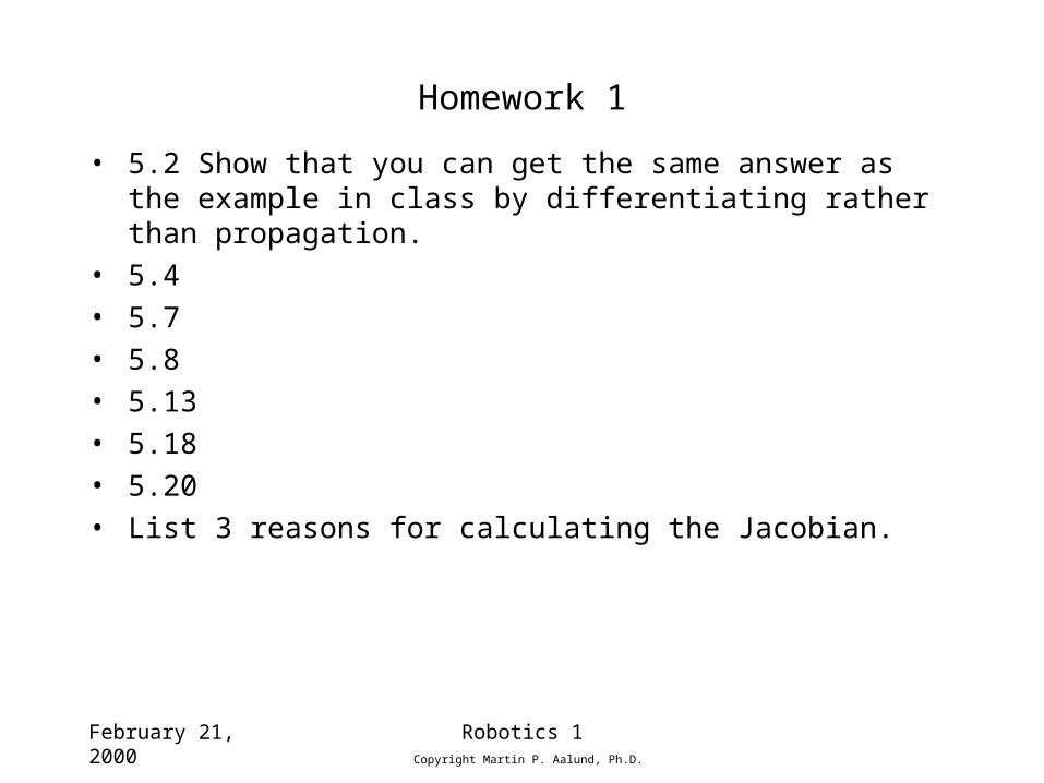
Homework 1

• 5.2 Show that you can get the same answer as the example in class by differentiating rather than propagation.

• 5.4

• 5.7

• 5.8

• 5.13

• 5.18

• 5.20

• List 3 reasons for calculating the Jacobian.

february 21, 2000robotics 1 copyright martin p. aalund, ph.d. computational considerations

Documents

copyright martin

b slide

velocity velocity

actual workspace slide

arcmate robot slide

reference frame velocity

radius of wrist sphere

shilling arm slide