federal planning bureau economic analyses and forecasts federal planning bureau economic analyses...

Federal Planning BureauEconomic analyses and forecasts

Federal Planning Bureau Economic analyses and forecasts

The option value approach in MIDAS_BE

Some work in progress

Jean-Charles Wijnandts1 and Raphaël Desmet2 and Gijs Dekkers3

1. University of Liège (student internship at the FPB)2. Federal Planning Bureau3. Federal Planning Bureau and Katholieke Universiteit

LeuvenPaper presented at the Ministero dell'Economia e delle Finanze, Rome, February 15th, 2011


The option value approach in MIDAS_BE: some work in progress

Overview of this presentation A very short introduction to the option value

approach

Why including the option value approach?

The current situation

How to include the option value approach in the alignment process?

Some very preliminary simulation results


A very short introduction to the option value approach*

* Note the word “approach” here.

The flow of expected future utilities can then be written as:

rbUayUarV sbrs

sts

sy

r

tss

tst

)(1

(1)

t the year of potential retirement r the year of actual retirement s future year, starting from either t or r ys labour income in year s bs(r) pension income in year s, given retirement in r Uy the utility of consumption Ub the utility of consumption in leisure β discount-factor =1/(1+discount rate) as the probability of survival from t to s

Given that r*= arg max(Vt(r)), it holds that Vt(r*)-Vt(r) > 0 for each year that r*≠ r. Considering all the future years that one can

choose to retire (i.e. from t to the year one reaches the mandatory retirement age), the option value in t is Gt(r*)=Vt(r*)-Vt(t), and one

will postpone retirement from year t for as long as Gt(r*)>0. In r*, there is no additional expected utility from working, and one will

therefore retire.


A very short introduction to the option value approach

The notion of actuarial neutrality involves setting the gains from postponing retirement by just one year against the associated lossesSOCIAL SECURITY WEALTH or SSW equals the flow of discounted expected utility

from retirement in the year r, as seen from t.

rs

sstst

r rbaSSW (1)

The WEALTH ACCRUAL is the change of SSW as a result of delaying retirement by just

one year

tr

tr

tr SSWSSWSSW 1 (2)

The IMPLICIT TAX ON WORKING LONGER is the ratio of expected losses (renounced

pension wealth) and gains (salary) for every year that retirement is postponed.

rrtr

trt

r ya

SSWitax

(3)




approach







The current version of MIDAS_Be has all kind of behavioural equations, but they lack any theoretical underpinning and have no explicit inclusion of retirement incentives.

The Belgian first-pillar employees’ pensions is highly actuarially non-neutral (Dekkers, IJM, 2007) and this affects the retirement decision (Dellis et al., in Gruber and Wise, 2004).

In the absence of an option value approach, the impact of any policy measure aiming to reduce actuarial imbalance on the retirement decision is likely to be underestimated by MIDAS.




approach






The labour market module in MIDAS_BE I


The labour market module in MIDAS_BE II


The labour market module in MIDAS_BE III

Table 1: Estimation results for labour market participation - Men

In work previous year Not in work previous year

Coef. Std. Err. Coef. Std. Err.

University -0.3270*** 0.1539 -0.2423** 0.1958

Upper secondary -0.2408*** 0.1345 -0.3555*** 0.1691

Ever had a job 0.7684*** 0.2552 0.9161*** 0.2278

Potential experience 0.0416*** 0.0191 -0.1876*** 0.0223

Potential experience2 -0.0026*** 0.0003 0.0013*** 0.0004

Chronically ill -0.5585*** 0.1302 -0.7686*** 0.1892

Other inactive (lag) - - -0.3428** 0.2147

Unemployed (lag) - - -0.9702*** 0.2043

Spouse in work (lag) - - 0.6741*** 0.2070

Intercept 4.7792*** 0.3414 2.1716*** 0.2758

Number of obs. 15395 2498

Pseudo R2 0.2018 0.3808

Notes: Coef. = coefficient; Std. Err. = standard error; * = p<0.10; ** = p<0.05; *** = p<0.01. Dashes indicate variables not included in the model.


The labour market module in MIDAS_BE IV

Table 2: Estimation results for labour market participation - Women

In work previous year Not in work previous year

Coef. Std. Err. Coef. Std. Err.

University 0.2296*** 0.1177 - -

Upper secondary - - -0.1860*** 0.1001

Ever had a job 0.4662*** 0.1706 0.7900*** 0.1344

Married 0.5570*** 0.1293 -0.7587*** 0.1324

Newly divorced/separated -0.6841*** 0.3636 0.6225** 0.3798

Number of children 0-11 -0.3441*** 0.0555 -0.3789*** 0.0585

Number of children 12-15 - - 0.1515** 0.0933

Potential experience -0.0387*** 0.0169 -0.1665*** 0.0166

Potential experience2 -0.0010*** 0.0003 0.0011*** 0.0003

Chronically ill -0.3916*** 0.1212 -0.5442*** 0.1409

Other inactive (lag) - - 0.1564*** -4.0400

Unemployed (lag) - - -0.3691*** 0.1670

Spouse in work (lag) -0.6413*** 0.1104 0.8166*** 0.1210

Intercept 5.1472*** 0.2700 1.6363*** 0.2107

Number of obs. 13333 6390

Pseudo R2 0.2050 0.2545

Notes: Coef. = coefficient; Std. Err. = standard error; * = p<0.10; ** = p<0.05; *** = p<0.01. Dashes indicate variables not included in the model.




approach







IN WORK

No

UNEMPLOYMENT

DISABILITY

EARLY-RETIREMENT, UNEMPLOYMENT FOR OLDER WORKERS, …

RETIREMENT

OTHER INACTIVE

Yes

)exp(1

)exp()(logit 1-

ii

iiiii X

XXr

Implicit tax on working longer

Alignment for people between 60 and 64

rrtr

trt

r ya

SSWitax

Alignment for people younger than 60




approach







Distribution of the implicit tax on work continuation for men and women at 60 and 64 in scenario 2

mean Nb of observations Scenario 2M60 -0.04774 129 Scenario 2M64 -0.18622 58 Scenario 2W60 -0.04013 150 Scenario 2W64 -0.05742 30

• Women have on average slightly higher implicit taxes than men

• Men and women selected at an earlier stage to stop their activity have higher implicit taxes on average than people selected at a later stage.



Average retirement benefits the year of labor market withdrawal for men and women at 60 and 64 in scenario 1 and 2

Mean Nb of observations

Scenario 1M60

15685.27 195

Scenario 2M60

14595.58 290

Scenario 1W60

14169.6 246

Scenario 2W60

13853.57 326

Scenario 1M64

20490.12 146

Scenario 2M64

17577.09 87

Scenario 1W64

18064.32 101

Scenario 2W64

17081.95 52



Proportion of men and women withdrawing from the labor market by age in scenario 1 and 2

60 61 62 63 64 Nb of observations Scenario 1 25.09 22.11 20.75 18.11 13.95 2352 Scenario 2 39.40 20.62 17.60 13.20 9.18 2114 Scenario 1M 22.31 21.34 19.63 20.68 16.04 1228 Scenario 2M 37.16 19.54 18.72 13.58 11.01 1090 Scenario 1W 28.11 22.95 21.98 15.30 11.65 1124

Scenario 2W 41.80 21.78 16.41 12.79 7.23 1024

The general trend is a strong increase of the market withdrawals at age 60 in scenario 2 at the expense of other ages between 61 and 64 years old


Some very preliminary simulation results: Gini coefficient


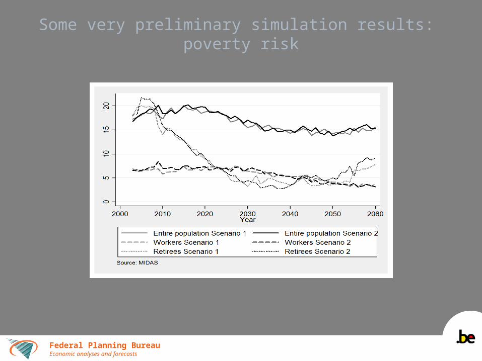
Some very preliminary simulation results: poverty risk


Conclusions This variant of MIDAS_BE applies the implicit tax to set the

ranking in the alignment of older workers

Men and women selected at an earlier stage to stop their activity have higher implicit taxes on average than people selected at a later stage.

The average pension benefit of the earliest and last leavers decrease as a result of introducing the implicit tax

The general trend is a strong increase of the market withdrawals at age 60 in scenario 2 at the expense of other ages between 61 and 64 years old

The rise in inequality among pensioners during the first two decades is less pronounced and inequality in generally lower when the implicit tax is introduced.

The impact of introducing the implicit tax on poverty risks is remarkably limited.

federal planning bureau economic analyses and forecasts federal planning bureau economic analyses...

Documents

option value approach

word approach

short introduction

current version of midas

progress overview

current situation

preliminary simulation

alignment process