An experimental analogue for memristor based Chua’s circuit

R. Jothimurugan∗ and K. Thamilmaran†

Centre for Nonlinear Dynamics, School of Physics,

Bharathidasan University, Tiruchirappalli-620 024, Tamilnadu, India

Ronilson Rocha‡

Federal University of Ouro Preto-UFOP/EM/DECAT,

Campus Morro do Cruzeiro, 35400-000, Ouro Preto, MG, Brazil.

(Dated: September 9, 2021)

Abstract

This paper presents the dynamics of a practical equivalent of a smooth memristor oscillator

derived from Chua’s circuit. This approach replaces the conventional Chua’s diode by a flux

controlled memristor with negative conductance. The central idea is to design a practical memristor

based circuit using electronic analogy in order to bypass problems related to the realization of

memristor equivalents. The amplitude and the frequency of the oscillations are previously defined

in the circuit design. The result is a robust and flexible circuit without inductors, which is able

to reproduce a rich variety of dynamical behaviors. The proposed analogue circuit is successfully

designed and implemented, producing experimental time series, phase portraits, and power spectra,

which are corroborated by numerical simulations. The “0-1 test” is also performed in order to verify

the regular and chaotic dynamics on the proposed analogue circuit.

Keywords: Memristor, Chua’s circuit, Electronic analogy, ‘0-1’ test

∗jothi@cnld.bdu.ac.in†maran.cnld@gmail.com‡rocha@em.ufop.br

1

arX

iv:1

408.

4905

v1 [

nlin

.CD

] 2

1 A

ug 2

014

I. INTRODUCTION

Leon O. Chua postulated the memristor in the year of 1971 based on the symmetry

arguments. It is believed to be the fourth fundamental passive circuit element followed

by the resistor, capacitor and inductor [1]. Memristor gets wide attention by the research

community after its physical realization by Stanley William’s group from HP labs in 2008

[2]. The memristor is a passive two-terminal electronic device described by a nonlinear

constitutive relation which is either one of the following two forms of the voltage-current

relationship, (i) v = M(q)i and (ii) i = W (φ)v. Here, the nonlinear functions M(q) and

W (φ) are regarded as memristance and memductance respectively, whose functional forms

are defined by M(q) = dφ(q)/dq and W (φ) = dq(φ)/dφ represent the slope of the scalar

functions φ = φ(q) and q = q(φ), respectively which are called memristor constitutive

relation [3].

The memristor has potential applications in physics, mathematics, engineering, biology,

and other various fields. Recent researches that involve synthesis of memristive devices

[2, 4], mathematical modeling and analysis [5–8], application of memristor theory to the

nano-battery [9], memory effects on light emitting diodes [10], memristive behavior of elec-

trical properties of the human skin [11], and synaptic connections among brain cell of the

human [12] explicitly demonstrate the potentiality of the memristor. In a nutshell, it can

be understood from the 18K+ citations registered for memristor in google scholar as on

01.07.2014 [13].

The analysis of nonlinear systems using experimental circuits is always an active area of

research that provides a better understanding on the theoretical concepts. The FitzHugh-

Nagumo circuit for neuron model [14, 15], the Lorenz oscillator based on a climate model

[16] and the popular Chua’s circuit [17] are few examples of this kind. In this context,

several studies are made on the development of memristor based circuits, since memris-

tors are commercially not available yet. For example, the analog integrator based smooth

memristor was implemented to study the behaviour of Chua’s circuit with memristor as

nonlinear element [18]. The time varying resistor based memristor circuit is implemented

on electronic circuit simulator to study the occurrence of chaotic beats in a driven Chua’s

circuit [19] and the nonsmooth bifurcations, transient hyperchaos and hyperchaotic beats in

a Murali-Lakshmanan-Chua circuit [20]. Apart from that, analogue circuits to explore the

2

voltage-current characteristic of the memristor are also reported in the literature [21, 22].

In all these studies, the memristor is separately conceived as a sub-circuit to follow the

specific choice of memristive function. All these sub-circuits are complex and prone to the

dynamical deviations from the mathematical modeling due to the tolerance effects of the

circuit components and the inherent noise effects. Further, all these reports having physical

inductors which are unwise to implement the circuits on PCB/VLSI designs.

In this paper, the smooth memristor based Chua’s circuit equation is implemented in

an experimental hardware in order to capture its dynamical behaviors on real time. The

circuit is designed using the concept of electronic analogy [23, 24]. The advantage of this

realization is that the amplitude of the each state variable can be scaled up/down according

to the application requirements, reducing the noise influence on the circuit dynamics. This

method of circuit implementation is straight forward and easy to implement with printed

circuit boards (PCBs) since it do not have physical or synthetic inductors. The functional

form of the memristor associated with this circuit is assumed to be smooth, continuous and

monotonically increasing nature. The proposed analogue circuit realization is versatile, sta-

ble, and it satisfactorily reproduces almost all simulated dynamics by numerical integration.

The experimental time series, phase portraits and power spectra are traced in real time on

digital storage oscilloscope, which are confirmed using numerical simulation. We also have

performed the newly developed “0-1” test to the experimental times series to distinguish the

regular and chaotic motion of the circuit dynamics. The parameter K results ‘0’ for regular

and ‘1’ for chaotic dynamics.

The rest of the paper is organized as follows: the original memristor based Chua’s circuit,

its state equations and the associated dynamics are discussed in Section 2. In Section 3, first

the procedure of amplitude scaling is explained and then, the method of constructing Chua’s

circuit using electronic analogy is described. The results of PSpice simulation, experimental

observation and the numerical integration studies are discussed in Section 4. In Section 5,

the “0-1 test” is performed using experimental time series data to verify the periodic and

chaotic dynamics of the circuit. Conclusions are given in section 6.

3

II. THE CHUA’S CIRCUIT WITH MEMRISTOR

The Figure 1 shows the memristor based Chua’s circuit. Here, NR is active nonlinear

element which comprises the parallel combination of negative conductance (−G) and two

terminal passive flux controlled memristor. The memristor is characterized by smooth con-

tinuous cubic monotonic-increasing nonlinearity given by [3, 18]:

q(φ) = aφ+ bφ3, (1)

where a and b are constants which are assumed to be greater than zero. From this expression,

the memductance W (φ) can be deduced as

W (φ) =dq(φ)

dφ= a+ 3bφ2. (2)

The circuit equation for memristor based Chua’s circuit can be written using Kirchoff’s

laws as follows [3],

dv1dt

=1

RC1

(v2 − v1 +GRv1 −RW (φ)v1), (3a)

dv2dt

=1

RC2

(v1 − v2 −RiL), (3b)

diLdt

= − 1

Lv2, (3c)

dφ

dt= v1, (3d)

where, v1, v2, i and φ are voltage across the capacitors C1, C2, current flowing through the

inductor L and the flux through the memristor respectively. Substituting the functional

form W (φ) in to Eq. 3(a) yields,

dv1dt

=1

RC1

(v2 − v1 +GRv1 −R(a+ 3bφ2)v1). (3e)

By applying transformation to the variables as x1 = v1, x2 = v2, x3 = iL, x4 = φ, α = 1/C1,

4

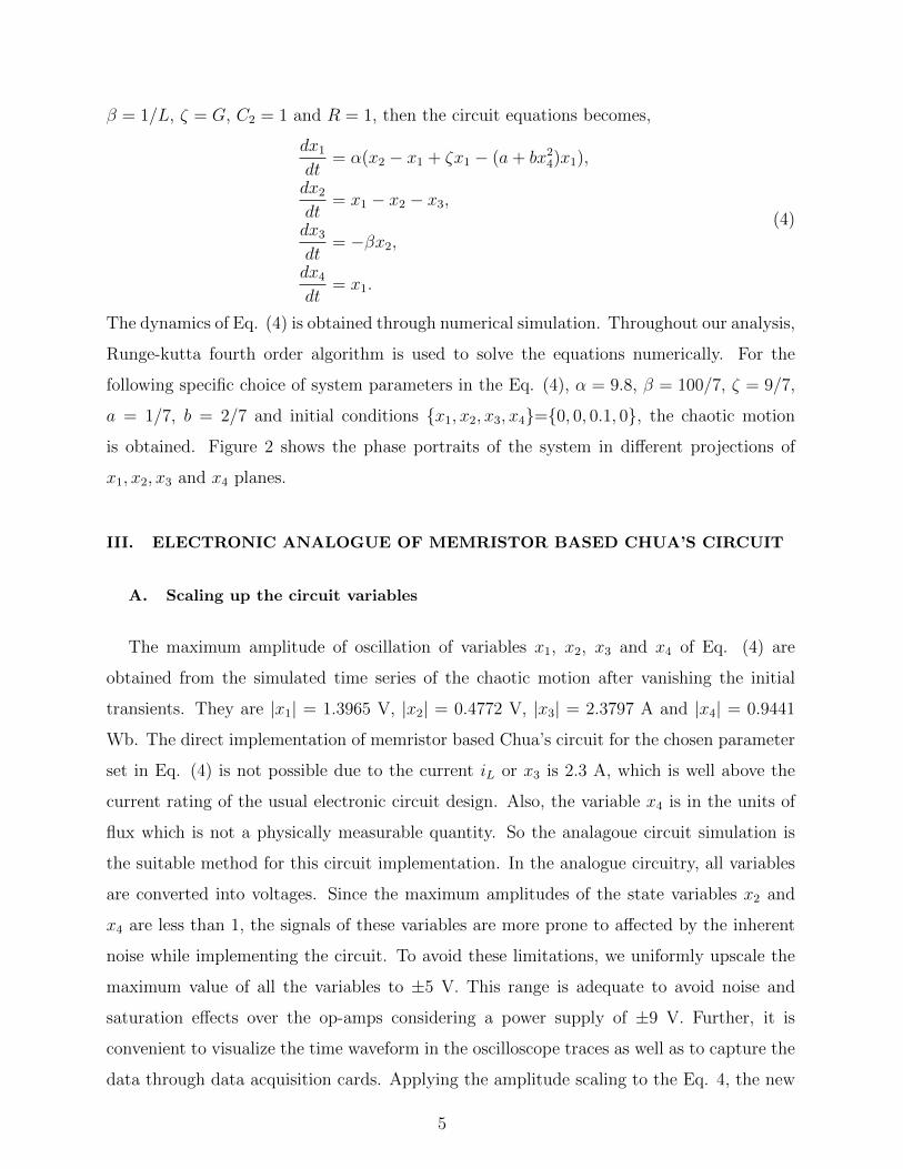
β = 1/L, ζ = G, C2 = 1 and R = 1, then the circuit equations becomes,

dx1dt

= α(x2 − x1 + ζx1 − (a+ bx24)x1),

dx2dt

= x1 − x2 − x3,

dx3dt

= −βx2,

dx4dt

= x1.

(4)

The dynamics of Eq. (4) is obtained through numerical simulation. Throughout our analysis,

Runge-kutta fourth order algorithm is used to solve the equations numerically. For the

following specific choice of system parameters in the Eq. (4), α = 9.8, β = 100/7, ζ = 9/7,

a = 1/7, b = 2/7 and initial conditions x1, x2, x3, x4=0, 0, 0.1, 0, the chaotic motion

is obtained. Figure 2 shows the phase portraits of the system in different projections of

x1, x2, x3 and x4 planes.

III. ELECTRONIC ANALOGUE OF MEMRISTOR BASED CHUA’S CIRCUIT

A. Scaling up the circuit variables

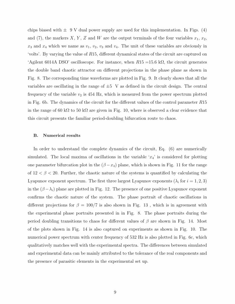
The maximum amplitude of oscillation of variables x1, x2, x3 and x4 of Eq. (4) are

obtained from the simulated time series of the chaotic motion after vanishing the initial

transients. They are |x1| = 1.3965 V, |x2| = 0.4772 V, |x3| = 2.3797 A and |x4| = 0.9441

Wb. The direct implementation of memristor based Chua’s circuit for the chosen parameter

set in Eq. (4) is not possible due to the current iL or x3 is 2.3 A, which is well above the

current rating of the usual electronic circuit design. Also, the variable x4 is in the units of

flux which is not a physically measurable quantity. So the analagoue circuit simulation is

the suitable method for this circuit implementation. In the analogue circuitry, all variables

are converted into voltages. Since the maximum amplitudes of the state variables x2 and

x4 are less than 1, the signals of these variables are more prone to affected by the inherent

noise while implementing the circuit. To avoid these limitations, we uniformly upscale the

maximum value of all the variables to ±5 V. This range is adequate to avoid noise and

saturation effects over the op-amps considering a power supply of ±9 V. Further, it is

convenient to visualize the time waveform in the oscilloscope traces as well as to capture the

data through data acquisition cards. Applying the amplitude scaling to the Eq. 4, the new

5

variables are defined as x1 = 3.3x1, x2 = 10x2, x3 = 2x3 and x4 = 5x4. Rewriting the Eq.

(4) to the new variables and dropping the bar over the variables for convenience, yields the

following upscaled system,

dx1dt

= α(0.33x2 − x1 + ζx1 − ax1 + 0.12bx24x1),

dx2dt

= 3.03x1 − x2 − 5x3,

dx3dt

= −0.2βx2,

dx4dt

= 1.5152x1.

(5)

Considering a probability of any intermediate signal to surpass the saturation voltage

limits, the entire system equation is then divided by the largest parameter. In the present

case, since the greatest parameter is β = 100/7 = 14.28, we divide the entire system by

the factor 15 on both sides of the Eq. (5). Although this procedure affects the operational

frequency of the circuit, it has not influence on the system dynamics. Hence, the rescalled

final set of equations are given by,

dx1dt

= 0.2156x2 + 0.09342x1 − 2.24109x24100

x1,

dx2dt

= 0.202x1 − 0.067x2 − 0.33x3,

dx3dt

= −0.0133βx2

dx4dt

= 0.10101x1.

(6)

In this rescaling, the parameter values used for numerical simulation of Eq. (4) is applied

for all the parameters except β, which is used to be the control parameter for the rest of the

study.

B. Implementation of analogue Memristor based Chua’s circuit

In the analogue computation, a first order differential equation can be solved primar-

ily using an weighted integrator. The dynamics of the memristor based Chua’s circuit is

described by a set of four first order coupled nonlinear differential equations as given in

Eq. (6). Hence, the analogue implementation of memristor based Chua’s circuit will have

6

four weighted integrators. Unit gain inverting amplifiers are used to change the sign of the

variables. To incorporate the nonlinear functional part present in the Eq. 6, the analogue

multipliers are used. Figure 3 shows these three fundamental cells namely (a) the weighted

inverting integrator, (b) scale changer (unit gain inverting amplifier) and (c) the multiplier

chip, used to realize the analogue memristor based Chua’s circuit. The transfer function of

the weighted integrator is given by

vo = − 1

RC

∫vinR∗

dt, (7)

where vin and v0 are the input and output voltages of the integrator respectively. The R∗

refers to the normalized value of the input resistance in relation to the base resistance R.

The frequency of the analogue circuit is determined by the value of the base resistance R

and the capacitance C. The sign of the any state variable can be electronically changed

using unit gain inverting amplifier. The transfer function of the inverting amplifier is,

vo = −vin, when Rin = Rf , (8)

where Rin and Rf are the input and feedback resistors of the amplifier unit. The analog

multiplier is useful component to multiply two analog signals. We use this component to

get the nonlinear part present in the Eq. 6. The product output W0 of a typical multiplier

can be written as,

W0 =(X1 −X2) ∗ (Y1 − Y2)

10+ Z, (9)

Here, X1 and X2 are X-multiplicand of non-inverting and inverting inputs, Y1 and Y2 are

Y -multiplicand of non-inverting and inverting inputs and Z is the summing input. The

dividing factor 10 is used to avoid the overflow of product output.

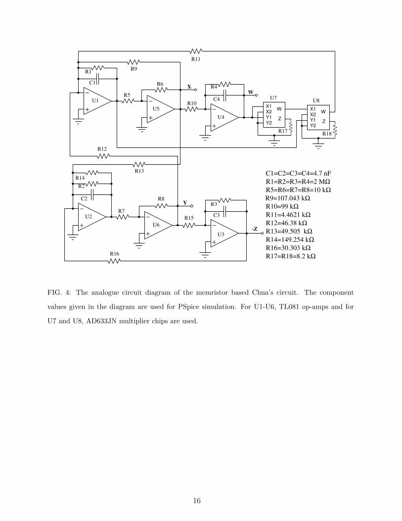
The analogue circuit to emulate the Eq. (6) is implemented using the above described

three electronic entities as shown in Fig. 4. In the circuit diagram U1, U2, U3 and U4

are the weighted integrators, U5 and U6 are inverting amplifiers and U7 and U8 represents

the multiplier chips. A feedback resistor with high value (R = 2 MΩ) is connected to each

integrator in order to fix the gain at low frequencies and to reduce the effect of the offset

voltages in the op-amps. This feedback resistor should be at least 10 times greater than the

input resistance of its respective integrator. For similar reasons, resistors are placed at the

Z terminals of the multipliers also.

7

The coefficients values values of the Eq. (6) are inversely proportional to R∗ values in the

circuit. To explain the calculation of the R∗ value from the coefficients of Eq. (6), we consider

last line in the Eq. (6). The variable x1 in the right hand side has the coefficient value

0.10101. The corresponding R∗ value to the input resistance of the W cell is 1/0.10101 = 9.9.

The value of corresponding resistor in the circuit is then directly calculated as (R∗xR) 9.9 x

10 kΩ = 99 kΩ. In the similar way, values of the resistance corresponding to all coefficients

in Eqns. (6) are obtained.

IV. RESULTS

A. Experimental results

On the implementation of analogous circuit, it is noticed that the calculated value of the

resistances are not fit with the off-the-shelf component values. Thus, the direct implemen-

tation of this circuit shown in Fig. 4 is firstly realized on the PSpice, a popular electronic

circuit simulation software. The component values given in Fig. 4 are used in PSpice sim-

ulation those are exactly the analogous to the numerical values. The double band chaotic

attractor on different phase projections obtained from the PSpice simulation are given in

Fig. 5 for R15 = 53.5 kΩ. Figure 6a shows the Fast Fourier Transform spctrum of the

variable ‘v2’. The measured central freqency in the FFT spectrum is 523 Hz. When the

resistances are adjusted for off-the-shelf values considering the hardware realization, the cir-

cuit dynamics remains unaltered. The PCB hardware circuit is shown in Fig. 7. The values

of the components are chosen as C1 = C2 = C3 = C4 = 4.7 nF, R1 = R2 = R3 = R4 =

2 MΩ, R5 = R6 = R7 = R8 = 10 kΩ, R9 = 106.8 kΩ, (R9A = 100 kΩ + R9B = 6.8 kΩ),

R10 = 100 kΩ, R11 = 4.46 kΩ, R12 = 47 kΩ, R13 = 49.2 kΩ, (R13A = 47 kΩ + R13B =

2.2 kΩ), R14 = 150 kΩ, R16 = 30 kΩ, (R16A = 10 kΩ + R16B=10 kΩ + R16C = 10 kΩ)

and R17 = R18 = 6.8 kΩ. These components may have the tolerance of 1% from the

standard value. To get the accurate reproduction of numerical results on experiment, the

resistors R9, R13, and R16 are split into parts whereby the sum of the resistors will yield

the closest possible value towards the numerical parameters. The variable resistor “R15”

will serve as the control parameter which is corresponding to β used as control parameter in

numerical analysis. The polyester type capacitors, TL081 op-amps and AD633JN multiplier

8

chips biased with ± 9 V dual power supply are used for this implementation. In Figs. (4)

and (7), the markers X, Y , Z and W are the output terminals of the four variables x1, x2,

x3 and x4 which we name as v1, v2, v3 and v4. The unit of these variables are obviously in

‘volts’. By varying the value of R15, different dynamical states of the circuit are captured on

‘Agilent 6014A DSO’ oscilloscope. For instance, when R15 =15.6 kΩ, the circuit generates

the double band chaotic attractor on different projections in the phase plane as shown in

Fig. 8. The corresponding time waveforms are plotted in Fig. 9. It clearly shows that all the

variables are oscillating in the range of ±5 V as defined in the circuit design. The central

frequency of the variable v2 is 454 Hz, which is measured from the power spectrum plotted

in Fig. 6b. The dynamics of the circuit for the different values of the control parameter R15

in the range of 60 kΩ to 50 kΩ are given in Fig. 10, where is observed a clear evidence that

this circuit presents the familiar period-doubling bifurcation route to chaos.

B. Numerical results

In order to understand the complete dynamics of the circuit, Eq. (6) are numerically

simulated. The local maxima of oscillations in the variable ‘x4’ is considered for plotting

one parameter bifurcation plot in the (β−x4) plane, which is shown in Fig. 11 for the range

of 12 < β < 20. Further, the chaotic nature of the systems is quantified by calculating the

Lyapunov exponent spectrum. The first three largest Lyapunov exponents (λi for i = 1, 2, 3)

in the (β−λi) plane are plotted in Fig. 12. The presence of one positive Lyapunov exponent

confirms the chaotic nature of the system. The phase portrait of chaotic oscillations in

different projections for β = 100/7 is also shown in Fig. 13 , which is in agreement with

the experimental phase portraits presented in in Fig. 8. The phase portraits during the

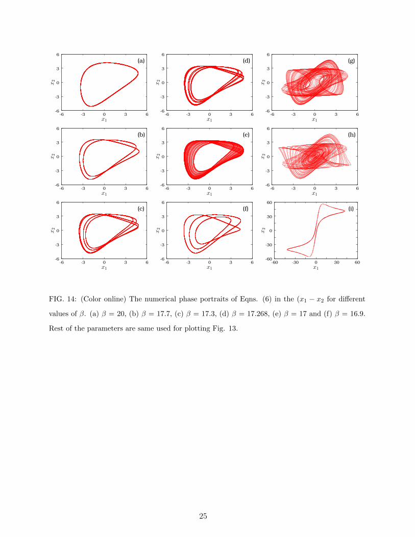
period doubling transitions to chaos for different values of β are shown in Fig. 14. Most

of the plots shown in Fig. 14 is also captured on experiments as shown in Fig. 10. The

numerical power spectrum with center frequency of 532 Hz is also plotted in Fig. 6c, which

qualitatively matches well with the experimental spectra. The differences between simulated

and experimental data can be mainly attributed to the tolerance of the real components and

the presence of parasitic elements in the experimental set up.

9

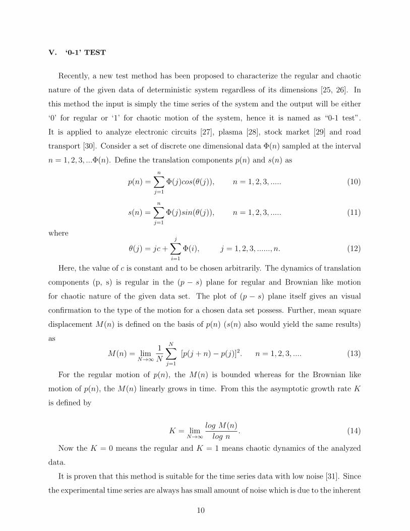
V. ‘0-1’ TEST

Recently, a new test method has been proposed to characterize the regular and chaotic

nature of the given data of deterministic system regardless of its dimensions [25, 26]. In

this method the input is simply the time series of the system and the output will be either

‘0’ for regular or ‘1’ for chaotic motion of the system, hence it is named as “0-1 test”.

It is applied to analyze electronic circuits [27], plasma [28], stock market [29] and road

transport [30]. Consider a set of discrete one dimensional data Φ(n) sampled at the interval

n = 1, 2, 3, ...Φ(n). Define the translation components p(n) and s(n) as

p(n) =n∑

j=1

Φ(j)cos(θ(j)), n = 1, 2, 3, ..... (10)

s(n) =n∑

j=1

Φ(j)sin(θ(j)), n = 1, 2, 3, ..... (11)

where

θ(j) = jc+

j∑i=1

Φ(i), j = 1, 2, 3, ......, n. (12)

Here, the value of c is constant and to be chosen arbitrarily. The dynamics of translation

components (p, s) is regular in the (p − s) plane for regular and Brownian like motion

for chaotic nature of the given data set. The plot of (p − s) plane itself gives an visual

confirmation to the type of the motion for a chosen data set possess. Further, mean square

displacement M(n) is defined on the basis of p(n) (s(n) also would yield the same results)

as

M(n) = limN→∞

1

N

N∑j=1

[p(j + n)− p(j)]2. n = 1, 2, 3, .... (13)

For the regular motion of p(n), the M(n) is bounded whereas for the Brownian like

motion of p(n), the M(n) linearly grows in time. From this the asymptotic growth rate K

is defined by

K = limN→∞

log M(n)

log n. (14)

Now the K = 0 means the regular and K = 1 means chaotic dynamics of the analyzed

data.

It is proven that this method is suitable for the time series data with low noise [31]. Since

the experimental time series are always has small amount of noise which is due to the inherent

10

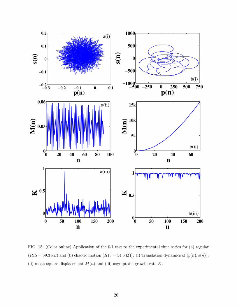
noise fluctuation present in the circuit itself. We perform the “0-1 test” for the experimental

data collected during the periodic and chaotic dynamics of the proposed circuit (Fig. 7). The

set of ‘n’data points of the time series ‘x4’ after the initial transients vanished, is collected

to the computer from the circuit using “Agilent-U2531A” data acquisition module with the

sampling rate of 500 kSa/s. The value of the constant ‘c’ is randomly varied between (0−π).

The calculated translation components (p, s), the mean square displacement M(n) and the

asymptotic growth rate K for regular (period-1 limit cycle at R15 = 59.3 kΩ) and chaotic

time series (double band chaotic attractor at R15 = 54.6 kΩ) are plotted in Fig. 15. These

plots clearly differentiates the regular and chaotic motion of the circuit.

VI. CONCLUSIONS

In this paper, the Chua’s circuit with smooth, cubic functional memristor is experi-

mentally designed and implemented. The difficulties on physical realization of memristor

sub-circuit are bypassed using a circuit design based in electronic analogy. To avoid the

inherent noise influence on variables oscillating on low amplitudes, the amplitude scaling is

applied to original circuit equations such that the maximum amplitude of the oscillations

is ±5V. This method of implementation is straight forward and it allows to reproduce all

possible dynamics captured in computational simulations. The designed circuit is flexible

and robust, presenting well comparable size in relation to other designs proposed in the

literature. The experimental implementation provides time waveforms, phase portraits, and

power spectra that present a good agreement with numerical simulation. Further, the nu-

merical simulation also confirms the period doubling bifurcation scenario identified in the

experiment. The regular and chaotic motion of the experimental data are clearly distin-

guished using “0-1 test”. In this context, the proposed analogue circuit can be used as a

prototype model for memristor based circuit, consisting in a good option for the investigation

of strange non-chaos, chaotic beats, nonlinear resonances and other associated behaviors.

Acknowledgments

The authors acknowledges the technical support of K. Suresh, S. Sabarathinam and P.

Megavarna Ezhilarasu during various stages of this work. R.J. is supported by the University

11

Grants Commission, India in the form of Research Fellowship in Science for Meritorious

Students. The work of K.T. forms a part of a Department of Science and Technology,

Government of India sponsored project grant no. SB/EMEQ-077/2013.

[1] Chua, L. O.: Memristor-The missing circuit element. IEEE Trans. Circuit Syst. 18(5), 507-519

(1971).

[2] Strukov, D. B., Snider, G. S., Stewart, D. R., Stanley Williams, R.: The missing memristor

found. Nature 453, 80-83 (2008).

[3] Itoh, M., Chua, L. O.: Memristor Oscillators. Int. J. Bifurcation and Chaos 18(11), 3183-3206

(2008).

[4] JoshuaYang, J., Pickett, M. D., Xuema Li, Ohlberg, D. A. A., Stewart, D. R., Stanley

Williams, R.: Memristive switching mechanism for metal/oxide/metal nanodevices. Nature

Nanotechnology 3 429-433 (2008).

[5] Botta, V. A., Nespoli, C., Messias, M.: Mathematical analysis of a third order memristor

based Chua’s oscillator. TEMA Tend. mat. Apl. Comput. 12(2), 91-99 (2011).

[6] Bao Bo-Cheng, Xu Jian-Ping, Liu Zhong: Initial state dependent dynamical behviours in a

memristor based chaotic circuit. Chin. Phys. Lett. 27(7), 070504 (2010).

[7] Teng, L., Iu, H. H. C., Wang, X., Wang, X.: Chaotic behaviour in fractional-order memristor-

based simplest chaotic circuit using fourth degree polynomial. Nonlinear Dyn. 77, 231-241

(2014).

[8] Slipko, V. A., Pershin, Y. V., Di Ventra, M.: Changing the state of a memristive system with

white noise. Phys. Rev. E 87, 042103 (2013).

[9] Valov, I., Linn, E., Tappertzhofen, S., Schmelzer, S., van den Hurk, J., Lentz, F., Waser, R.:

Nanobatteries in redox-based resistive switches require extension of memristor theory. Nature

Communications. 4, 1771 (2013).

[10] Zakhidov, A. A., Byungki Jung, Slinker, J. D., Abruna, H. D., Malliaras, G. G.: A light-

emitting memristor. Organic Electronics. 11, 150-153 (2010).

[11] Martinsen, O. G., Grimnes, S., Lutken, C. A., Johnsen, G. K.: Memristance in human skin.

J. Phys.: Conference Series 224, 012071 (2010).

[12] Andy Thomas: Memristor-based neural networks. J. Phys. D: Appl. Phys. 46, 093001 (2013).

12

[13] http://scholar.google.co.in/citations?user=Yc4TtpUAAAAJ&hl=en

[14] Bordet, M., Morfu, S.: Experimental and numerical study of noise effects in a FitzHugh-

Nagumo system driven by a biharmonic signal. Chaos Solitons and Fractals 54, 82-89 (2013).

[15] Bordet, M., Morfu, S., Marquie, P.: Ghost stochastic resonance in FitzHugh-Nagumo circuit.

Elect. Lett. 50(12), 861-862 (2014).

[16] Blakely, J. N., Eskridge, M. B., Corron, N. J.: A simple Lorenz circuit and its radio frequency

implementation. Chaos 17, 023112 (2007).

[17] Chua, L. O., Komuro, M., Matsumoto, T.: The double scroll family. IEEE Trans. Circuit.

Syst. 33(11), 1072-1118 (1986).

[18] Muthuswamy, B.: Implementing memristor based Chaotic circuits. Int. J. Bifurcation Chaos

20(5), 1335-1350 (2010).

[19] Ishaq Ahamed, I., Srinivasan, K., Murali, K., Lakshmanan, M.: Observation of chaotic beats

in a driven memristive Chua’s circuit. Int. J. Bifurcation Chaos. 21(3), 737- 757 (2011).

[20] Ishaq Ahamed, I., Lakshmanan, M.: Nonsmooth bifurcations, transient hyperchaos and hyper-

chaotic beats in a memristive Murali-Lakshmanan-Chua’s circuit. Int. J. Bifurcation Chaos.

23(6), 1350098 (2013).

[21] Bao Bo-Cheng, Feng Fei, Dong Wei and Pan Sai-Hu: The voltage-current relationship and

equivalent circuit implementation of parallel flux-controlled memristive circuits. Chin. Phys.

B 22(6), 068401 (2013).

[22] Juraj Valsa, Dalibor Biolek and Zdenek Biolek: An analogue model of the memristor. Int. J.

Numer. Model. 24, 400-408 (2011).

[23] Rocha, R., and Medrano-T, R. O.: An inductor-free realization of the Chua’s circuit based on

electronic analogy. Nonlinear Dyn. 56, 389-400 (2009).

[24] Rocha, R., Martins Filho, L. S., machado, R. E.: A methodology for teaching of dynamical

systems using analogue electronic circuits. Int. J. Electr. Eng. Educ. 43, 334-345 (2006).

[25] Gottwald, G. A., Melbourne, I.: A new test for chaos in deterministic systems. Proc. R. Soc.

Lon. A 460, 603-611 (2004).

[26] Ke-Hui, S., Xuan, L., Cong-Xu, Z.: The 0-1 test algorithm for chaos and its applications.

Chin. Phys. B 19(11), 110510 (2010).

[27] Cafagna, D., Grassi, G.: Fractional-order Chua’s circuit: Time-domain analysis, bifurcation,

chaotic behavior and test for chaos. Int. J. Bifurcation and Chaos 18, 615 (2008).

13

[28] Chowdhury, D. R., Iyengar, A. N. S., Lahiri, S.: Gottwald Melborune (0-1) test for chaos in

plasma. Nonlin. Processes Geophys. 19, 53-56, 2012.

[29] Webel, K.: Chaos in German stock returns-New evidence from 0-1 test. Economics Letters

115, 487-489 (2012)

[30] Krese, B., Govekar, E.: Analysis of traffic dynamics on a ring road-based transportation

network by means of 0-1 test for chaos and Lyapunov spectrum. Transportation Research

Part C 36, 27-34 (2013).

[31] Kulp, C. W., Smith, S.: Characterization of noisy symbolic time series. Phys. Rev. E 83

026201 (2011).

iC2

v1

R

C2 C1

iC1

v2

++

+

_ _ _L

iL

-G

i

v

Flux controlled

memristor

NR

FIG. 1: The Chua’s circuit with memristor (NR).

14

(a)

x1

x2

1.50.750-0.75-1.5

0.50

0.25

0.00

-0.25

-0.50

(b)

x1

x3

1.50.750-0.75-1.5

2.5

1.5

0.0

-1.5

-2.5

(c)

x1

x4

1.50.750-0.75-1.5

1.0

0.5

0.0

-0.5

-1.0

(d)

x2

x3

0.500.250-0.25-0.50

2.5

1.5

0.0

-1.5

-2.5

(e)

x2

x4

0.500.250-0.25-0.50

1.0

0.5

0.0

-0.5

-1.0

(f)

x3

x4

2.51.50-1.5-2.5

1.0

0.5

0.0

-0.5

-1.0

FIG. 2: (Color online) Different projections of phase portraits in the (a) (x1 − x2), (b) (x1 − x3),

(c) (x1−x4), (d) (x2−x3), (e) (x2−x4) and (f) (x3−x4) planes obtained numerically from Eqns.

4. The parameters of the system are fixed as α = 9.8, β = 100/7, γ = 9/7, a =1/7 and b =2/7.

The initial conditions are x1, x2, x3, x4=0, 0, 0.1, 0.

−

+

Vin

Vo

CRin

OA

(a)

(b)

−

+

−

+

−

+

OA

OA

OA

Z

(c)

1/10

−

+

Vin

Vo

Rin

OA

Rf

X1

X2

Y1

Y2

W0

FIG. 3: The fundamental units of the analogue computation. Namely, (a) the integrator, (b) the

inverting amplifier and (c) the schematic of an analog multiplier.

15

−

+

−

+

−

+

−

+

−

+

−

+

X1

X2

Y1

Y2

W

Z

X1

X2

Y1

Y2

W

Z

R1

R2

R3

R4

R5

R6

R7

R8

R9

R10

R11

R12

R13

R14

R15

R16

R17R18

C1

C2

C3

C4

U2

U1

U3

U4

U5

U6

U7U8

X

Y

-Z

C1=C2=C3=C4=4.7 nF

R1=R2=R3=R4=2 MΩ

R5=R6=R7=R8=10 kΩ

R9=107.043 kΩ

R10=99 kΩ

R11=4.4621 kΩ

R12=46.38 kΩ

R13=49.505 kΩ

R14=149.254 kΩ

R16=30.303 kΩ

R17=R18=8.2 kΩ

W

FIG. 4: The analogue circuit diagram of the memristor based Chua’s circuit. The component

values given in the diagram are used for PSpice simulation. For U1-U6, TL081 op-amps and for

U7 and U8, AD633JN multiplier chips are used.

16

FIG. 5: Different projections of PSpice simulated phase portraits in the (a) (v1−v2), (b) (v1−v3),

(c) (v1 − v4), (d) (v2 − v3), (e) (v2 − v4) and (f) (v3 − v4) planes.

17

FIG. 6: (Color online) Fast Fourier transform spectrum of the variable v2 for different simulation

platforms with central operating frequency. (a) PSpice circuit simulation : 523 Hz, (b) Hardware

circuit : 454 Hz, Scale: Horizontal axis = 200 Hz/div, Vertical axis = 10dB/div and (c) Numerical

simulation : 532 Hz.

18

FIG. 7: (Color online) Experimental setup of the memristor based Chua’s circuit. U1-U6 are

TL081 op-amps, U7,U8 are AD633 mulitipliers. The nodes ‘X’, ‘Y’, ‘Z’ and ‘W’ are outputs of the

circuit. The variable resistor “R15” is used as a control parameter.

FIG. 8: (Color online) Different projections of phase portraits obtained from experiment in the (a)

(v1 − v2), (b) (v1 − v3), (c) (v1 − v4), (d) (v2 − v3), (e) (v2 − v4) and (f) (v3 − v4) planes. Scale:

Horizontal axis = 1.36 V/div, Vertical axis = 1.52 V/div.

19

FIG. 9: (Color online) Experimental time waveform of the variables v1(t), v2(t), v3(t) and v4(t).

Scale: Horizontal axis = 5 mS/div, Vertical axis = (a) 2.5 V/div, (b) 3.0 V/div, (c) 4.0 V/div and

(d) 2.5 V/div.

20

FIG. 10: (Color online) Period doubling scenario of experimental phase portraits in the (v1 − v2)

plane. (a) period-1 limit cycle (R15 = 59.3 kΩ), (b) period-2 limit cycle (R15 = 57.2 kΩ), (c )

period-4 limit cycle (R15 = 55.9 kΩ), (d) single band chaos (R15 = 55.1 kΩ), (e) double band

chaos (R15 = 54.6 kΩ) and (f) saturated limit cycle (R15 = 53.1 kΩ).

21

181716

β

x4

2018161412

5

2

-1

-4

FIG. 11: (Color online) The one parameter diagram in the (β − x4) plane obtained by numerical

simulation. The period doubling sequence is clearly captured in the inset.

22

β

λi

2018161412

1.5

1.0

0.5

0

-0.5

-1.0

-1.5

FIG. 12: (Color online) The Lyapunov exponents spectrum for first three exponents (λi for i = 1, 2

and 3) are plotted in the (β−λi) plane. The fourth exponent is skipped to view the rest conveniently.

The positive values in the λ1 indicates the chaotic nature of the system.

23

(a)

x1

x2

630-3-6

6

3

0

-3

-6

(b)

x1

x3

630-3-6

6

3

0

-3

-6

(c)

x1

x4

630-3-6

6

3

0

-3

-6

(d)

x2

x3

630-3-6

6

3

0

-3

-6

(e)

x2

x4

630-3-6

6

3

0

-3

-6

(f)

x3

x4

630-3-6

6

3

0

-3

-6

FIG. 13: (Color online) The numerical phase portraits of Eqns. (6) in the (a) (x1 − x2), (b)

(x1 − x3), (c) (x1 − x4), (d) (x2 − x3), (e) (x2 − x4) and (f) (x3 − x4) planes. The parameters of

the system are fixed as α = 9.8, β = 100/7, γ = 9/7, a =1/7 and b =2/7. The initial conditions

are x1, x2, x3, x4=0, 0, 1.0, 0.

24

(a)

x1

x2

630-3-6

6

3

0

-3

-6

(d)

x1

x2

630-3-6

6

3

0

-3

-6

(g)

x1

x2

630-3-6

6

3

0

-3

-6

(b)

x1

x2

630-3-6

6

3

0

-3

-6

(e)

x1

x2

630-3-6

6

3

0

-3

-6

(h)

x1

x2

630-3-6

6

3

0

-3

-6

(c)

x1

x2

630-3-6

6

3

0

-3

-6

(f)

x1

x2

630-3-6

6

3

0

-3

-6

(i)

x1

x2

60300-30-60

60

30

0

-30

-60

FIG. 14: (Color online) The numerical phase portraits of Eqns. (6) in the (x1 − x2 for different

values of β. (a) β = 20, (b) β = 17.7, (c) β = 17.3, (d) β = 17.268, (e) β = 17 and (f) β = 16.9.

Rest of the parameters are same used for plotting Fig. 13.

25

−0.3 −0.2 −0.1 0 0.1−0.2

−0.1

0

0.1

0.2

p(n)

s(n)

−500 −250 0 250 500 750−1000

−500

0

500

1000

p(n)

s(n)

0 20 40 60 80 1000

0.03

0.06

n

M(n)

0 20 40 600

5k

10k

15k

n

M(n)

0 50 100 150 200

0

0.5

1

n

K

0 50 100 150 2000

0.5

1

n

K

a(i)

a(ii)

a(iii)

b(i)

b(ii)

b(iii)

FIG. 15: (Color online) Application of the 0-1 test to the experimental time series for (a) regular

(R15 = 59.3 kΩ) and (b) chaotic motion (R15 = 54.6 kΩ): (i) Translation dynamics of (p(n), s(n)),

(ii) mean square displacement M(n) and (iii) asymptotic growth rate K.

26