feedback control for optimal process operation · feedback control for optimal process operation...

www.elsevier.com/locate/jprocont

Journal of Process Control 17 (2007) 203–219

Feedback control for optimal process operation

Sebastian Engell *

Lehrstuhl fur Anlagensteuerungstechnik (Process Control Laboratory), Department of Biochemical and Chemical Engineering,

Universitat Dortmund, D-44221 Dortmund, Germany

Received 22 July 2006; received in revised form 27 October 2006; accepted 27 October 2006

Abstract

In chemical process operation, the purpose of control is to achieve optimal process operation despite the presence of significant uncer-tainty about the plant behavior and disturbances. Tracking of set-points is often required for lower-level control loops, but on the pro-cess level in most cases this is not the primary concern and may even be counterproductive. In this paper, different approaches how torealize optimal process operation by feedback control are reviewed. The emphasis is on direct optimizing control by optimizing an eco-nomic cost criterion online over a finite horizon where the usual control specifications in terms of, e.g., product purities enter as con-straints and not as set-points. The potential of this approach is demonstrated by its application to a complex process whichcombines reaction with chromatographic separation. Issues for further research are outlined in the final section.� 2006 Elsevier Ltd. All rights reserved.

Keywords: Optimizing control; Finite horizon optimization; Control of integrated processes

Contents

1. Introduction . . . . . . . . . . . . . . . . . . . . . . . . . . . . . . . . . . . . . . . . . . . . . . . . . . . . . . . . . . . . . . . . . . . . . . . . . . . . . . . 2042. Optimization by regulation (self-optimizing control) . . . . . . . . . . . . . . . . . . . . . . . . . . . . . . . . . . . . . . . . . . . . . . . . . . . 2043. Real-time optimization (RTO) . . . . . . . . . . . . . . . . . . . . . . . . . . . . . . . . . . . . . . . . . . . . . . . . . . . . . . . . . . . . . . . . . . 2064. Reducing the gap between regulation and RTO . . . . . . . . . . . . . . . . . . . . . . . . . . . . . . . . . . . . . . . . . . . . . . . . . . . . . . 208

0959-1

doi:10.

* TelE-m

4.1. Frequent RTO . . . . . . . . . . . . . . . . . . . . . . . . . . . . . . . . . . . . . . . . . . . . . . . . . . . . . . . . . . . . . . . . . . . . . 2084.2. Integration of steady-state optimization into model-predictive control . . . . . . . . . . . . . . . . . . . . . . . . . . . . . . . . 2084.3. Integration of nonlinear steady-state optimization in the linear MPC controller . . . . . . . . . . . . . . . . . . . . . . . . . 209

5. Direct finite horizon optimizing control . . . . . . . . . . . . . . . . . . . . . . . . . . . . . . . . . . . . . . . . . . . . . . . . . . . . . . . . . . . . 210
5.1. General ideal . . . . . . . . . . . . . . . . . . . . . . . . . . . . . . . . . . . . . . . . . . . . . . . . . . . . . . . . . . . . . . . . . . . . . . 2105.2. Case study: control of reactive simulated moving bed chromatographic processes . . . . . . . . . . . . . . . . . . . . . . . . 210
5.2.1. Process description. . . . . . . . . . . . . . . . . . . . . . . . . . . . . . . . . . . . . . . . . . . . . . . . . . . . . . . . . . . . . 2105.2.2. Control of SMB processes. . . . . . . . . . . . . . . . . . . . . . . . . . . . . . . . . . . . . . . . . . . . . . . . . . . . . . . . 2115.2.3. Online optimizing control . . . . . . . . . . . . . . . . . . . . . . . . . . . . . . . . . . . . . . . . . . . . . . . . . . . . . . . . 2115.2.4. The Hashimoto reactive SMB process . . . . . . . . . . . . . . . . . . . . . . . . . . . . . . . . . . . . . . . . . . . . . . . . 2115.2.5. Optimizing controller application . . . . . . . . . . . . . . . . . . . . . . . . . . . . . . . . . . . . . . . . . . . . . . . . . . . 212

5.3. Numerical aspects . . . . . . . . . . . . . . . . . . . . . . . . . . . . . . . . . . . . . . . . . . . . . . . . . . . . . . . . . . . . . . . . . . . 213
6. Open issues . . . . . . . . . . . . . . . . . . . . . . . . . . . . . . . . . . . . . . . . . . . . . . . . . . . . . . . . . . . . . . . . . . . . . . . . . . . 214
6.1. Modeling . . . . . . . . . . . . . . . . . . . . . . . . . . . . . . . . . . . . . . . . . . . . . . . . . . . . . . . . . . . . . . . . . . . . . . . . . 2146.2. Stability. . . . . . . . . . . . . . . . . . . . . . . . . . . . . . . . . . . . . . . . . . . . . . . . . . . . . . . . . . . . . . . . . . . . . . . . . . 2156.3. State estimation . . . . . . . . . . . . . . . . . . . . . . . . . . . . . . . . . . . . . . . . . . . . . . . . . . . . . . . . . . . . . . . . . . . . 215

524/$ - see front matter � 2006 Elsevier Ltd. All rights reserved.

1016/j.jprocont.2006.10.011

.: +49 2317555126.ail address: [email protected]

mailto:[email protected]

204 S. Engell / Journal of Process Control 17 (2007) 203–219

6.4. Measurement-based optimization. . . . . . . . . . . . . . . . . . . . . . . . . . . . . . . . . . . . . . . . . . . . . . . . . . . . . . . . . 2156.5. Reliability and transparency . . . . . . . . . . . . . . . . . . . . . . . . . . . . . . . . . . . . . . . . . . . . . . . . . . . . . . . . . . . . 2166.6. Effort vs. performance . . . . . . . . . . . . . . . . . . . . . . . . . . . . . . . . . . . . . . . . . . . . . . . . . . . . . . . . . . . . . . . . 216

7. Conclusions. . . . . . . . . . . . . . . . . . . . . . . . . . . . . . . . . . . . . . . . . . . . . . . . . . . . . . . . . . . . . . . . . . . . . . . . . . . . . . . . 216Acknowledgements. . . . . . . . . . . . . . . . . . . . . . . . . . . . . . . . . . . . . . . . . . . . . . . . . . . . . . . . . . . . . . . . . . . . . . . . . . . . 216

References . . . . . . . . . . . . . . . . . . . . . . . . . . . . . . . . . . . . . . . . . . . . . . . . . . . . . . . . . . . . . . . . . . . . . . . . . . . . . . . . 217

1. Introduction

From a process engineering point of view, the purposeof automatic feedback control (and that of manual controlas well) is not primarily to keep the controlled variables attheir set-points as well as possible or to nicely trackdynamic set-point changes, but to operate the plant suchthat the net return is maximized in the presence of distur-bances and uncertainties, exploiting the available measure-ments. The model used for plant design will usually notrepresent the real process exactly so that an operatingregime that was optimized for the plant model does notlead to an optimal operation of the real plant, but mayeven be infeasible. Feedback control, automatic or manual,is indispensable to handle the inaccuracies and uncertain-ties that are present in the design process, and to make fulluse of the capacity of the equipment. This has been pointedout in a number of papers (see e.g. [1–5]) but nonethelessalmost all of the literature on automatic control and con-troller design for chemical processes is concerned with thetask to make certain controlled variables track given set-points or set-point trajectories while assuring closed-loopstability. In chemical process control, however, good track-ing of set-points is mostly of interest for lower-level controltasks. This contributes to the attitude of managers and pro-cess engineers to consider the choice and the tuning of con-trollers as a necessary but uninteresting task, comparableto the procurement and maintenance of pumps or valvesfor a predefined purpose, which should be performed ascheaply as possible.

In their plenary lecture at ADCHEM 2000, Backx et al.[6] stressed the need for dynamic operations in the processindustries in an increasingly marked-driven economy whereplant operations are embedded in flexible supply chainsstriving at just-in-time production in order to maintaincompetitiveness. Minimizing operation cost while main-taining the desired product quality in such an environmentis considerably harder than in a continuous productionwith infrequent changes, and this cannot be achieved solelyby experienced operators and plant managers using theiraccumulated knowledge about the performance of theplant. Profitable agile operation calls for a new look onthe integration of process control with process operations.In this contribution, we give a review of the state of the artin integrated process optimization and control of continu-ous processes and highlight the option of direct or onlineoptimizing control (also called one-layer approach [7] orfull optimizing control [8]).

First the idea to implement the optimal plant operationby conventional feedback control, termed ‘‘self-optimizingcontrol’’ [5], is discussed in Section 2. In highly automatedplants, the goal of an economically optimal operation isusually addressed by a two-layer structure [9] which is dis-cussed in Section 3. On the upper layer, the operating pointof the plant is optimized based upon a rigorous nonlinearstationary plant model (real-time optimization, RTO).The optimal operating point is characterized by set-pointsfor a set of controlled variables that are passed to lower-level controllers that keep the chosen variables as close tothese set-points as possible by manipulating the availabledegrees of freedom of the process within certain bounds.This two-layer structure has some drawbacks. As the opti-mization is only performed intermittently at a low sam-pling rate, the adaptation of the operating conditions isslow. Inconsistencies may arise from the use of differentmodels on the different layers. These issues are partlyaddressed by schemes in which the economic optimizationis integrated within a linear MPC controller on the lowerlevel, as discussed in Section 4.

Recent progress in algorithms for numerical simulationand optimization enables to move from the two-layerarchitecture to direct online optimizing control. In thisapproach, the available degrees of freedom of the processare directly used to optimize an economic cost functionalover a certain prediction horizon based upon a rigorousnonlinear dynamic process model. The regulation of qual-ity parameters, which is usually formulated as a tracking ordisturbance rejection problem, can be integrated into theoptimization by means of additional constraints that haveto be satisfied over the prediction horizon. The applicabil-ity of this integrated approach is demonstrated for theoperation of simulated moving bed chromatographic pro-cesses. Finally, open issues and possible lines of futureresearch are discussed.

2. Optimization by regulation (self-optimizing control)

The idea behind what was termed ‘‘self-optimizing con-trol’’ by Skogestad [5] has been outlined already in [1]: afeedback control structure should have the property thatthe adjustments of the manipulated variables that areenforced by keeping some function of the measured vari-ables constant are such that the process is operated at theeconomically optimal steady state in the presence of distur-bances. Morari et al. [1] stated that the objective in the syn-thesis of a control structure is ‘‘to translate the economic

S. Engell / Journal of Process Control 17 (2007) 203–219 205

objectives into process control objectives’’, a point of viewthat has thereafter found surprisingly little attention inthe literature on control structure selection. A sub-goal inthis ‘‘translation’’ is to select the regulatory control struc-ture of a process such that steady-state optimality of pro-cess operations is realized to the maximum extentpossible if the selected controlled variables are driven tosuitably chosen set-points. In the approach describedbelow, the selection is done solely with respect to the sta-tionary process performance, the consideration of thedynamics of the controlled loops follows as a second step.This reflects that from a plant operations point of view, acontrol structure that yields nice transient responses andtight control of the selected variables may be useless oreven counterproductive if keeping these variables at theirset-points does not improve the economic performance ofthe process. The goal of the control structure selection isthat in the steady state a similar performance is obtainedas it would be realized by optimizing the stationary valuesof the operational degrees of freedom of the process forknown disturbances and parameter variations. Thus therelation between the manipulated variables u and the dis-turbances di, ucon = f(yset,di) which is (implicitly) realizedby regulating the chosen variables to their set-points shouldbe an approximation of the optimal input uopt(di). Theapplication of this idea to the selection of control structureshas been demonstrated in a number of application papers[10–12].

The effect of feedback control on the profit function J inthe presence of disturbances can be expressed as [12]

DJ ¼ Jðunom; d ¼ 0Þ � Jðunom; diÞþ Jðunom; diÞ � Jðuopt; diÞ þ Jðuopt; diÞ � Jðucon; diÞ:

ð1Þ

Fig. 1. Schematic representation of the influence of a disturbance on theprofit for different control approaches in the presence of measurementerrors. J(unom): performance for nominal inputs, J(uopt): performance foroptimal inputs, J(ucon): performance under feedback control with andwithout measurement errors.

The first term is the loss due to disturbances that would berealized if the manipulated variables were fixed at theirnominal values. The second term represents the effect ofan optimal adaptation of the manipulated variables tothe disturbance di, and the third term is the difference ofthe optimal compensation of the disturbance and the com-pensation which is achieved by the chosen feedback controlstructure. If the first term in (1) is much larger (in absolutevalue) than the second one, or if all terms are relativelysmall, then a variation of the manipulated variables offersno advantage, and neither optimization nor feedback con-trol is required for this disturbance. If the third term is notsmall compared to the attainable profit for optimized in-puts for all possible regulating structures, then online opti-mization or an adaptation of the set-points should beperformed rather than just regulation of the chosen vari-ables to fixed pre-computed set-points.

Eq. (1) represents the loss (which may also be negative,i.e. a gain) of profit for one particular disturbance di and afixed control structure. The economic performance of acontrol structure can then be measured by

DJ ¼Z d1;max

�d1;max

Z dn;max

�dn;max

wðdÞðJðunom; dÞ � Jðucon; dÞdd1 � � � ddn;

ð2Þ

where w(d) is the probability of the occurrence of the dis-turbance vector d, neglecting the effect of potential con-straint violations. As feedback control is based onmeasurements, errors in the measurements of the con-trolled variables must be taken into account. A variablemay be very suitable for regulatory control in the sense thatthe resulting inputs are a good approximation of the opti-mal inputs, but due to a large measurement error or a smallsensitivity to changes in the inputs, the resulting values ucon

may differ considerably from the desired values. This wasconsidered in an approximative fashion by checking thesensitivity of the profit with respect to the controlled vari-ables in [5]. An alternative is to consider the worst case con-trol performance for regulation of the controlled variablesto values in a range around the nominal set-point yset whichis defined by the measurement errors [12]. For a distur-bance scenario di, the performance measure of a controlstructure is

minu

Jðu; di; xÞ

s:t: _x ¼ f ðu; di; xÞ ¼ 0;

y ¼ mðxÞ ¼ Mðu; diÞ;yset � esensor 6 y 6 yset þ esensor;

ð3Þ

where f represents the plant dynamics. A regulatory controlstructure that yields a comparatively small value of theminimal profit is not able to guarantee the desired perfor-mance of the process in the presence of measurement errorsand hence is not suitable. This formulation includes thepractically relevant situation where closed-loop controlleads to a worse result than keeping the manipulated vari-ables constant at their nominal value. This will usually bethe case for small disturbances, as illustrated by Fig. 1,


where the effect of disturbances of different magnitudes onthe performance of a process is illustrated for fixed nominalinputs, optimized inputs, and feedback control with andwithout measurement errors. For small disturbances, keep-ing the controlled inputs at their set-points is better thanreacting to disturbed measurements of y. It is thereforeimportant to include scenarios with small disturbancesand not only those with very large ones into the set of dis-turbances that are considered in the analysis of the self-optimizing capacity of a control structure.

Application studies have shown that the profit loss thatis incurred by using regulation to fixed set-points instead ofsteady-state optimization can be quite low for well-chosencontrol structures. For example in [10] a performance lossof less than 5% is reported for the Tennessee Eastmanbenchmark problem [13].

The analysis described above and the control structureselection process that follows from it so far are limited todisturbances or variations of the plant behavior that persistover a very large period of time compared to the plantdynamics. The inclusion of disturbances with a higherbandwidth into the analysis as well as the integration withthe dynamic aspects of control structure selection is still anopen issue.

3. Real-time optimization (RTO)

A well-established approach to create a link betweenregulatory control and optimization of the economics ofthe unit or of the plant under control is real-time optimiza-tion (RTO) (see e.g. [9], and the references therein). AnRTO system is a model based, upper-level control systemthat is operated in closed loop and provides set-points tothe lower-level control systems in order to maintain theprocess operation as close as possible to the economic opti-mum. The general structure of an RTO system is shown inFig. 2. Its hierarchical structure follows the ideas put for-ward already in the 1970s, e.g. by Findeisen, et al. [14].

Planning and Scheduling

SS optimization Model update

Validation Reconciliation

C1 Cn

Plant

RTO

Fig. 2. Hierarchical control structure with real-time optimization (RTO),C1� � �Cn denote the local regulatory controllers.

The planning and scheduling system provides produc-tion goals (e.g. demands of products, quality parameters),parameters of the cost function (e.g. prices of products,raw materials, energy costs) and constraints (e.g. availabil-ity of raw materials), and the process control layer providesplant data on the actual values of all relevant variables ofthe process. This data is first analyzed for stationarity ofthe process and, if a stationary situation is confirmed, rec-onciled using material and energy balances to compensatefor systematic measurement errors. The reconciled plantdata is used to compute a new set of model parameters(including unmeasured external inputs) such that the plantmodel represents the plant as accurately as possible at thecurrent (stationary) operating point. Then new values forcritical state variables of the plant are computed whichoptimize an economic cost function while meeting the con-straints imposed by the equipment, the product specifica-tions, and safety and environmental regulations as well asthe economic constraints imposed by the plant manage-ment system. These values are filtered by a supervisory sys-tem (which usually includes the plant operators) (e.g.checked for plausibility, mapped to ramp changes, clippedto avoid large changes, etc. [15]) and forwarded to the pro-cess control layer which uses these values as set-points andimplements appropriate moves of the operational degreesof freedom (manipulated variables). For a discussion ofthe implementation of the optimal steady states by linearmodel-predictive controllers see the paper by Rao andRawlings [16].

As the RTO system employs a stationary process modeland the optimization is only performed if the plant isapproximately in a steady state, the time between succes-sive RTO steps must be large enough for the plant to reacha new steady state after the last commanded move. Thusthe sampling period must be several times the largesttime-constant of the controlled process. Reported samplingtimes are usually on the order of magnitude of several (4–8)hours or once per day.

The introduction of an RTO system provides a clearseparation of concerns and of time-scales between theRTO system and the process control system. The RTO sys-tem optimizes the plant economics on a medium time-scale(shifts to days) while the control system provides trackingand disturbance rejection on shorter time-scales from sec-onds to hours. Often the control system is again dividedinto separate layers in order to handle different speeds ofresponses and to structure the system into smaller modules.This separation of concerns however may be misunder-stood by the plant management leading to the erroneousconclusion that dynamics do not matter and that the hard-and software on the process control layer is a necessarypiece of equipment that is necessary to run the processbut it is the RTO system that helps to earn money.

In [17,18], a performance metric for RTO systems, calleddesign cost, was introduced where the profit obtainedby the use of the RTO system is compared to an estimateof the theoretical profit obtained from a hypothetical


delay-free static optimization and immediate implementa-tion of the optimal set-points without concern for the plantdynamics. The cost function consists of three parts:

• the loss in the transient period before the layered systemconsisting of the RTO system and the process controllayer has reached a new steady state,

• the loss due to model errors in the steady state,• the loss due to the propagation of stochastic measure-

ment errors to the optimized set-points.

The last contribution to the loss calls for a filtering ofthe changes before they are applied to the real plant toavoid inefficient moves [19,20]. The issue of model fidelitywas discussed in detail in [18,21]. In general, the use of arigorous model is recommended. Adequacy of a modelrequires that the gradient and the curvature of the profitfunction are described precisely whereas its absolute valueis not critical [22,23]. As parameter estimation is a core partof an RTO system, the commanded set-point changes havean influence on the model accuracy and hence on the close-ness to the true optimum. Yip and Marlin [24] made thevery interesting proposal to include the effect of set-pointchanges on the accuracy of the parameter estimates intothe RTO optimization.

The issue of (steady-state or iterative) optimization withinaccurate models has been addressed since long in the lit-erature. Roberts and co-workers proposed several algo-rithms that combine parameter re-estimation with the useof empirical gradients obtained from small perturbationsof the plant operation to account for structural plant-model mismatch [25–27]. Cheng and Zafiriou [28] proposeda modification of the FFSQ optimization algorithm [29] forsteady-state optimization on the RTO layer such that theobserved plant performance is taken into account whenthe search direction and the step size are computed butavoids the use of empirical gradients. Convergence to theoptimum can be assured even for considerable structuralplant-model mismatch, resulting from the use of simplifiedprocess models that do not satisfy the conditions for a suf-ficiently accurate model as formulated in [22].

Compared to running a plant with fixed set-points for theregulatory control layer, the introduction of the RTO layersignificantly increases the complexity of the control systemand causes additional costs in design, implementation andmaintenance. Thus the question arises, whether it pays offor not. Duvall and Riggs [30], in the evaluation of the per-formance of their RTO scheme for the Tennessee EastmanChallenge Problem pointed out: ‘‘RTO profit should be com-

pared to optimal, knowledgeable operator control of the pro-

cess to determine the true benefits of RTO. Plant operators,through daily control of the process, understand how process

set-point selection affects the production rate and/or operat-

ing costs’’. In particular, they state that the operators wouldmost likely know which variables should be kept at theirbounds but they will not be able to optimize set-pointswithin their admitted ranges according to the disturbances

encountered. This comparison therefore is quite similar tothe comparison with a well chosen, ‘‘self-optimizing’’ regu-latory control structure without RTO. In the example, a sig-nificant improvement by RTO was found.

Quoting the famous Dutch soccer player and coachJohan Cruyff, ‘‘every advantage is also a disadvantage’’.The advantage of the RTO/MPC structure is that it pro-vides a clear separation between the tasks of the controland the optimization layer. This separation is performedwith respect to time-scales as well as to models. Rigorousnonlinear models are used only on the steady-state optimi-zation layer. Such models nowadays are often availablefrom the plant design phase, so the additional effort todevelop the model sometimes is not very high. The controlalgorithms are based upon linear models (or no models atall if conventional controllers are tuned in simulations oron-site) which can be determined from plant data. Aspointed out by, e.g., Backx et al. [6]) and Sequeira et al.[31] this implies however that the models on the optimiza-tion layer and on the control layer will in general not befully consistent, in particular their steady-state gains maydiffer.

The main disadvantage of the RTO approach is thedelay of the optimization which is inevitably encounteredbecause of the steady-state assumption. After the occur-rence of a disturbance the optimization has to be delayeduntil the controlled plant has settled into a new steadystate. To detect whether the plant is in a steady state itselfis not a simple task (see e.g. [32]).

Suppose a step disturbance occurs in some unmeasuredexternal input to the plant. Then first the control systemwill regulate the plant (to the extent possible) to the set-points that were computed before the disturbanceoccurred. After all control loops have settled, the RTOoptimizer can be started, and after the results have beencomputed (which may also require a considerable amountof time, depending on the complexity of the model used)and validated, the control layer can start to regulate theplant to the new set-points. Thus it will take several timesthe settling time of the control layer to drive the plantto the new optimized mode of operation. In the first phase,the control system will try hard to maintain the previouslyoptimal operating conditions even if without fixing the con-trolled variables to their set-points the operation of theplant would have been more profitable. If the disturbancepersists for one sampling period of the RTO system plusone settling time of the regulatory layer, it can be estimatedthat the use of the RTO system on the average recoversabout half of the difference between the profit obtainedby the regulatory system alone (with fixed set-points) andan online-optimizing controller that implements the opti-mal set-points within the settling time of the regulatorycontrol layer. The combined RTO/regulatory controlstructure will work satisfactorily for infrequent stepchanges of feeds, product specifications or product quanti-ties but it will provide no benefit for changes that occur attime scales below the RTO sampling period.

Steady-state RTOslow sampling

QP/LP setpoint optimizationfast sampling

Linear constrained MPCfast sampling

Plant

costconstraints

setpoints

MVs

MVsCVs

MVsCVs

CVs

Fig. 3. Two-layer MPC with set-point optimization.


Marlin and Hrymak [9] listed several areas for improve-ment of RTO systems. Two important ones are alsoaddressed in the remainder of this paper: the integrationwith the process control layer, and the extension todynamic operation. They pointed out that instead of send-ing set-points to the control layer, an ideal RTO systemshould output a design (i.e. tuning parameters or even achoice of the control structure) of the control system thatleads to an optimized performance under the currentlong-term operating conditions.

4. Reducing the gap between regulation and RTO

4.1. Frequent RTO

As a consequence of the drawback that RTO is appliedwith rather long sampling periods, several authors have pro-posed schemes that use smaller sampling times on the opti-mizing layer. For example, Sequeira et al. [31] proposed tochange the set-points for the regulatory layer in muchshorter intervals (in the case study presented they used 1/50 of the settling time of the plant) and to perform a ‘‘real-time evolution’’ of the set-points by heuristic search (usedhere to reduce the computation time) based upon the sta-tionary process model and the available measurements. Toavoid overshooting behavior, the steps of the decision vari-ables are bounded in each step. In the example shown, thisscheme outperforms steady-state RTO with regulatory con-trol especially for non-stationary disturbances and in thefirst phase after a disturbance occurs, which is not too sur-prising. The idea that a ‘‘step in the right direction’’ shouldbe better than to wait until the process has settled to a newsteady state is certainly convincing, however the approachsuffers from neglecting the dynamics of the plant. Basaket al. [33] discussed an online optimizing control schemefor a complex crude distillation unit. They proposed to per-form a steady-state optimization of the unit for an economiccost function under constraints on the product propertieswith respect to the operational degrees of freedom and amodel parameter update at a sampling rate of 1–2 h and toapply the computed manipulated values directly to theplant. If the update of the manipulated variables is basedsolely on information on the plant inputs and the economics,such a scheme will react to disturbances only via the modelparameter update. If dynamic variables enter the optimiza-tion, the resulting dynamics of the controlled plant will beunpredictable from the stationary behavior. The idea to per-form updates of the operating point using a stationarymodel more frequently than every few settling times of theplant but to limit the size of the changes that are appliedto the plant such that quasi-stationary transients are realizedis also used in industrial practice. This leads to the imple-mentation of the optimal set-point changes by ramps ratherthan steps or, in other terms, of a nonlinear integral control-ler, causing slow moves of the overall system.

If a fast sampling RTO scheme is used, it will, at leastfor very short sampling times, interact with the regulatory

control layer causing uncontrolled effects because the sepa-ration of the time scales does no longer hold. The assump-tion that a steady-state optimization performed at aninstationary operating point yields the right move of theset-points is similar to the basic idea of gain schedulingcontrol. In both cases, a projection of the actual dynamicstate on a corresponding stationary point that is definedby the values of the measured, actuated or demanded vari-ables during transients is performed and the control moveis computed under the (in principle wrong) assumption thatthe plant actually is in this steady state. Fast samplingRTO thus shares the potential of stability problems withgain scheduling controllers which usually can only beavoided if ‘‘slow’’, quasi-stationary set-point changes arerealized (see e.g. [34,35]).

4.2. Integration of steady-state optimization

into model-predictive control

In order to narrow the gap between the low frequencynonlinear steady-state optimization performed on theRTO layer and the relatively fast linear MPC layer, theso-called LP-MPC and QP-MPC two-stage MPC struc-tures are frequently used in industry [36–41]. A detailedanalysis of their properties was given by Ying and Joseph[42]. The extended structure is shown in Fig. 3.

The task of the upper MPC layer is to compute the set-points (targets) both for the controlled variables and forthe manipulated inputs for the lower MPC layer by solvinga constrained linear or quadratic optimization problem,using information from the RTO layer and from theMPC layer. The optimization is performed with the samesampling period as the lower-level MPC controller. At eachsampling instant, the minimization

minyset ;uset

½ðyset � y�ÞT Cyðyset � y�Þ þ ðuset � u�ÞT Cuðuset � u�Þ

þ cyðyset � y�Þ þ cuðuset � u�Þ� ð4Þ


Subject to yset ¼ ASuset þ dðkÞ;dðkÞ ¼ dðk � 1Þ þ DðkÞ; ð5Þymin 6 yset 6 ymax;

umin 6 uset 6 umax

is performed.The steady-state gain AS and the disturbance estimate

are provided by the MPC layer whereas the nominal set-points y* and u* are provided by the RTO layer. This struc-ture addresses the following issues:

• A faster change of the set-points after the occurrence ofdisturbances is realized;

• The inconsistency of the nonlinear steady-state modelon the RTO layer and the linear steady-state model usedon the MPC layer is reduced;

• Large set-point changes that may drive the linear con-trollers unstable are avoided;

• The distribution of the offsets from the desired targetsthat are realized by the MPC controller is explicitly con-trolled and optimized.

The plant model and the disturbance estimate used onthe intermediate optimization layer is the same as that used(and eventually updated) on the MPC layer, thus avoidinginconsistencies, whereas the weights in the cost functionand the linear constraints are chosen such that theyapproximate the nonlinear cost function and the con-straints on the RTO layer around the present operatingpoint. As long as this approximation is good, optimal oper-ations are ensured.

A simpler approach to the integration of steady-stateoptimization and model-predictive control is to optimizethose tuning parameters of a dynamic matrix controller(DMC) or a QDMC controller that determine the steady-state behavior of the controller (set-points of the regulatedvariables, targets of the manipulated variables, weights onthe deviations of the regulated variables from the set-pointsand on the deviations of the of the manipulated variablesfrom the targets) such that the profit obtained is maximizedover a number of disturbance scenarios as proposed byKassidas et al. [43]. In the parameter optimization, a fullnonlinear steady-state plant model is used. Note that thisoptimization is only performed once (off-line), and onlythe usual computations of the DMC or QDMC controllermoves employing linear plant models have to be performedonline. The approach was compared to rigorous steady-state optimization (similar to what a RTO layer workingtogether with a zero-offset controller would yield) of thepurity set-points and to a controller that controls the plantto fixed pre-computed purity set-points (also optimizedover the various disturbance scenarios) for a simple distil-lation example. The optimization approach led to a consid-erable variation of the controlled outputs over the differentscenarios, while when the process is regulated to fixedset-points, this variation is mapped to the manipulated

variables. The optimally tuned DMC controller imple-ments a compromise between these extremes and realizesabout 70% of the average additional profit that resultsfor rigorous optimization. Even better results can beexpected for examples where the optimal operation ismostly determined by the constraints.

4.3. Integration of nonlinear steady-state optimization

in the linear MPC controller

Zanin et al. [7,44] reported the formulation, solutionand industrial implementation of a combined MPC/opti-mizing control scheme for a fluidized-bed catalytic cracker,FCC. The plant has seven manipulated inputs and six con-trolled variables. The economic criterion is the amount ofLPG produced. The optimization problem that is solvedin each controller sampling period is formulated in a mixedmanner: range control MPC with a fixed linear plant model(imposing soft constraints on the controlled variables by aquadratic penalty term that only becomes active when theconstraints are violated) plus a quadratic control movepenalty plus an economic objective that depends on the val-ues of the manipulated inputs at the end of the controlhorizon:

minDuðkþiÞ; i¼0;...;m�1

Xp

j¼1

kW 1ðyðkþ jÞ� rÞk22þXm�1

i¼0

kW 2Duðkþ iÞk22

þW 3fecoðuðkþm�1ÞÞþkW 4ðuðkþm�1Þ

�uðk�1Þ�DuðkÞÞk22þW 5½fecoðuðkþm�1Þ;yðkþ1ÞÞ

� fecoðuðkÞ;y0ðkþ1ÞÞ�2: ð6Þ

The value of the economic objective feco is computed usinga nonlinear steady-state process model. As only the firstmove of the controller is implemented, penalty terms areadded that penalize the deviation of the first values of themanipulated variables from their final values within thecontrol horizon in order to prevent that the economicallyoptimal control move is always ‘‘shifted to infinity’’. Sev-eral variants for this penalty term were investigated. Thedifferent components of the cost function were weightedsuch that the economic criterion and the MPC part havea similar influence on the values of the overall cost.

This combined optimizing/LMPC controller was imple-mented and tested at a real Petrobras FCC with a samplingrate of 1 min, a control horizon of two steps and a predic-tion horizon of 20 steps. An impressive performance isreported, both in terms of the economic performance andof the smoothness of the transients, pushing the processto its limits. The integrated control scheme performed sub-stantially better than the conventional scheme where theoperators chose set-points based on their experiences thatwere then implemented by a conventional MPC scheme.The final weights of the different contributions to the costfunction were determined by experiments. Simulations alsoshowed that the one-layer approach compared favorably to


a two-layer approach in which the economic optimizationprovided set-points for a linear MPC scheme in terms ofdynamic response. Nonetheless, the optimizing controllerwas not implemented in daily operation. The reasons willbe discussed below. A similar control scheme was experi-mentally validated in [45] for a paste dryer.

Fig. 4. Simulated moving bed principle.

5. Direct finite horizon optimizing control

5.1. General ideal

For demanding applications, the replacement of linearMPC controllers by nonlinear model-predictive control isa promising option and industrial applications have beenreported in particular in polymerization processes [46–49]. If nonlinear model-based control is used to implementoptimal set-points or optimal trajectories at a plant, it isonly a small step to replace the traditional quadratic costcriterion that penalizes the deviations of the controlledvariables from the reference values and the input variationsby an economic criterion. Constraints on outputs (e.g.strict product specifications) as well as process limitationscan then be included directly in the optimization problem.This approach has several advantages over a combinedsteady-state optimization/linear MPC scheme:

• Fast reaction to disturbances, no waiting for the plant toreach a steady state is required;

• Regulation of constrained variables to set-points whichimplies a safety margin between these set-points andthe constraints is avoided, the exact constraints can beimplemented for measured variables and only the modelerror has to be taken into account for unmeasured con-strained variables;

• Over-regulation is avoided, no variables are forced tofixed set-points and all degrees of freedom can be usedto optimize process performance;

• No inconsistency arises from the use of different modelson different layers;

• Economic goals and process constraints do not have tobe mapped to a control cost whereby economic optimal-ity is lost and tuning is difficult;

• The overall scheme is structurally simple.

An important point in favor of using an economic costcriterion and formulating restrictions of the process andthe product properties as constraints is that this reducesthe need for tuning of the weights in less explicit formula-tions. Exxon’s technology for NMPC employs a combina-tion of criteria that represent reference tracking, operatingcost and control moves [48].

In the next section, it will be demonstrated that directonline optimizing control can successfully be applied tocontrol problems that are hard to tackle by conventionalcontrol techniques. Other application studies have beenreported, e.g. by Singh et al. [50] and Johansen and Sbar-

baro [51] for blending processes and by Busch et al. [52]for a waste-water treatment plant.

5.2. Case study: control of reactive simulated moving bed

chromatographic processes

5.2.1. Process description

Chromatographic separations are a widespread separa-tion technology in the fine chemicals, nutrients and phar-maceutical industry. Chromatography is applied fordifficult separation tasks, in particular if the volatilities ofthe components are similar or if the valuable componentsare sensitive to thermal stress. The separation of enantio-mers (molecules that are mirror images of each other) isan example where chromatography is the method ofchoice. The standard chromatographic process is a batchseparation where pulses of the mixture that has to be sep-arated are injected into a chromatographic column fol-lowed by the injection of pure solvent. The componentstravel through the column at different speeds and can becollected at the end of the column in different purified frac-tions. In batch mode, the adsorbent is not used efficientlyand the process usually leads to highly diluted products.

The goal of a continuous operation of chromatographicseparations with a counter-current movement of the solidphase and the liquid phase led to the development of thesimulated moving bed (SMB) process by Broughton, [53].It is gaining increasing attention in industry due to itsadvantages in terms of productivity and solvent consump-tion [54,55]. An SMB process consists of several chromato-graphic columns connected in series which constitute aclosed loop. An effective counter-current movement ofthe solid phase relative to the liquid phase is achieved byperiodically and simultaneously moving the inlet and theoutlet lines by one column in the direction of the liquidflow (see Fig. 4).

After a start-up phase, SMB processes reach a periodicor cyclic steady state (CSS). The length of a cycle is equalto the duration of a switching period times the number ofcolumns, but relative to the port positions, the profilesare repeated every switching period. Fig. 5 shows the con-centration profiles of a binary separation along the col-

Fig. 5. Concentration profiles of an SMB process. The figure shows theconcentration profiles at different instances during one switching period.At the end of the period, the ports are switched.


umns plotted for different time instants within a switchingperiod.

5.2.2. Control of SMB processes

Classical feedback control strategies are not directlyapplicable to SMB processes due to their mixed discreteand continuous dynamics, spatially distributed state vari-ables with steep slopes, and slow and strongly nonlinearresponses of the concentrations profiles to changes of theoperating parameters. A summary of different approachesto control of SMB processes can be found in [56,57].

Klatt et al. [58] proposed a two-layer control architec-ture similar to the RTO/MPC scheme where the optimaloperating trajectory is calculated at a low sampling rateby dynamic optimization based on a rigorous processmodel. The model parameters are adapted using onlinemeasurements. The low level control task is to keep theconcentrations in the columns near the values at the opti-mal cyclic steady state despite disturbances, plant degrada-tion and plant/model mismatch. This is achieved bycontrolling the positions of the four concentration frontsin the process. The controller is based on input/outputmodels that are identified using simulation data producedby the rigorous process model near the optimal cyclicsteady state [58,59]. A disadvantage of this two-layer con-cept is that keeping the front positions at the valuesobtained from the rigorous optimization does not guaran-tee the product purities if structural plant/model mismatchoccurs. To ensure the specified product purities, an addi-tional purity controller is required, and the overall schemebecomes quite complex without actually ensuring optimaloperation because the lower-level controllers change theoptimized inputs in a suboptimal fashion.

5.2.3. Online optimizing control

As the progress in efficient numerical simulation andoptimization enabled a dynamic optimization of an SMB-process within one switching period, a direct finite hori-zon optimizing control scheme that employs the samerigorous nonlinear process model that is used for process

optimization in the two-layer structure was proposed andapplied to a 3-zones reactive SMB process for glucoseisomerization [60,61]. The key feature of this approach isthat the production cost is minimized online over a finitehorizon while the product purities are considered as con-straints, thus a real online optimization of all operationaldegrees of freedom is performed, and there is no trackingof pre-computed set-points or reference trajectories. In[62], this control concept was extended to the more com-plex processes VARICOL [63,64] and PowerFeed [65]where the ports are switched asynchronously and the flowrates are varied in the subintervals of the switching period.These process variants offer an even larger number ofdegrees of freedom that can be used for the optimizationof the process economics while satisfying the requiredproduct purities. In the optimizing control scheme pro-posed in [60,61], the states of the process model are deter-mined by forward simulation starting from measurementsin the recycle stream and in the product streams.

A different optimization-based approach to the controlof SMB processes was proposed by Erdem et al., [66–68].In their work, a moving horizon online optimization is per-formed based on a linear reduced-order model that isobtained from linearizing a rigorous model around theperiodic steady state. The state variables of the model areestimated by a Kalman Filter that processes the productconcentration measurements. Due to the use of repetitiveMPC [69] where the sampling time is equal to the switchingtime, the switching period has to be kept fixed which maycause a loss of performance compared to the optimizationof all available degrees of freedom.

5.2.4. The Hashimoto reactive SMB process

The integration of chemical reactions into chromato-graphic separations offers the potential to improve theconversion of equilibrium limited reactions. By the simulta-neous removal of the products from the reaction zone, thereaction equilibrium is shifted to the side of the products.This combination of reaction and chromatographic separa-tion can be achieved by packing the columns of the SMBprocess uniformly with adsorbent and catalyst, which leadsto the reactive SMB (SMBR) process. The SMBR processcan be advantageous in terms of higher productivity incomparison to a sequential arrangement of reaction andseparation units [70]. However, for equilibrium reactionsof the type A M B, a uniform catalyst distribution in theSMBR promotes the backward reaction near the productoutlet which is detrimental to the productivity. Furtheron, the renewal of deactivated catalyst is difficult when itis mixed with adsorbent pellets, and the same operatingconditions must be chosen for separation and reactionwhat may lead to either suboptimal reaction or suboptimalseparation. The Hashimoto SMB process [71,72] over-comes the disadvantages of the SMBR by performingseparation and reaction in separate units that containonly adsorbent or only catalyst. In this configuration, theconditions for reaction and for separation can be chosen

QDe ExQ

switching ofseparators

liquid flow

zone II zone IIIzone I zone IV

QRaQFe

recycle

Fig. 6. Four-zone Hashimoto reactive SMB process. White: separationunits, black: reactor units.


separately and the reactors can constantly be placed insome of the separation zones of the SMB process by appro-priate switching. The structure of a Hashimoto SMB pro-cess is shown in Fig. 6. The dynamics of this class ofprocesses is highly complex.

5.2.5. Optimizing controller application

The example application that will briefly be described inthe sequel is the racemization of Troger’s Base (TB) in com-bination with a chromatographic separation in order toproduce of the enantiomer TB – that is used for the treat-ment of cardiovascular diseases. More details can be foundin [73,74]. The solvent is an equimolar mixture of aceticacid that acts as the catalyst for the reaction and 2-propa-nole that increases the solubility of the mixture. Theadsorption of the Troger’s Base system to the solid phasecan be described by an adsorption isotherm that is ofmulti-component Langmuir type:

qi ¼H icp;i

1þP

kbi;kcp;k; k ¼ þ;�: ð7Þ

Here cp,i denotes the concentration of component i in thepores of the particle phase and qi the adsorbed fraction.The reaction takes place in plug flow reactors that are oper-ated at 80 �C whereby the catalyst is thermally activated. Inthe chromatographic columns that have a temperature of25 �C the catalyst is virtually deactivated. In the simulationrun shown below, a four-zone Hashimoto process witheight chromatographic columns, two reactors, and a col-umn distribution as shown in Fig. 6 is considered. Theobjective of the optimizing controller is to minimize the sol-vent consumption QDe for a constant feed flow and a givenpurity requirement in the presence of a plant/model mis-match. The inevitable mismatch between the model andthe behavior of the real plant is taken into account by feed-back of the difference of the predicted and the measuredproduct purities. A regularization term is added to theobjective function to obtain smooth trajectories of the in-put variables. The controller has to respect the purityrequirement for the extract flow which is averaged overthe prediction horizon, the dynamics of the HashimotoSMB model and the maximal flow rate in zone I due to lim-ited pump capacities. In order to guarantee that at least

70% of the mass of the components fed to the plant leavesthe plant in the extract product stream (averaged over theprediction horizon), an additional productivity require-ment was added. The resulting mathematical formulationof the optimization problem is

minbIi;bIIi

;bIIIi;bIVi

XHP

i¼1

QDeiþ DbiRDbi

s:t:~xk

smb ¼ xksmb þ

R st¼0

fsmbðxsmbðtÞ;bðtÞÞdt;

xkþ1smb ¼ P~xk

smb;

(

PHP

i PurEx;i

HP

P ðPurEx;min � DPurExÞ;PHP

i mEx;i

H P

P 0:7mFe � DmEx;

QI 6 Qmax;

QDe;QEx;QFe;QRe P 0;

ð8Þ

where the purity error DPurEx and the mass error DmEx arecalculated according to

DPurEx ¼ PurEx;plant;i�1 � PurEx;model;i�1;

DmEx ¼ mEx;plant;i�1 � mEx;model;i�1:ð9Þ

The model of the plant consists of rigorous dynamic mod-els of the individual columns of the plant and the nodeequations (represented by the function fsmb) and the portswitching (represented by the permutation matrix P). Thedegrees of freedom of the optimization problems are thetransformed flow rates bI–bIV in the four zones of the pro-cess which depend on the ratios of the flow rates of the li-quid phase in the zones to the effective solid flow rate thatis defined by the switching period s [58]. HP denotes theprediction horizon. The chromatographic columns are de-scribed by the general rate model [75] which accounts forall important effects of a radially homogeneous column,i.e. mass transfer between the liquid and the solid phase,pore diffusion, and axial dispersion. The partial differentialequations are discretized using a Galerkin approach on fi-nite elements for the bulk phase and orthogonal colloca-tion for the particle phase [76]. The reactors consist ofthree columns in series. Each column is discretized into12 elements, yielding an overall model with 1400 dynamicstates. For the solution of the optimization problem, thefeasible path solver FFSQ [29] is applied. It first searchesfor a feasible operating point and then minimizes the objec-tive function. The number of iterations of the SQP solverwas limited to 5 because the optimizer can perform at leastthis number of iterations within one cycle of the process(eight switching periods), as required for online control.If convergence is not achieved within five iterations, thebest feasible solution obtained is applied.

In the simulation scenario, a model/plant mismatch wasintroduced by disturbing the initial Henry coefficients H+

and H� of the model by +5% and �4%. The parametersof the controller are displayed in Table 1.

Table 1Controller parameters

Sampling time 1 cycle = 8 periodsPrediction horizon, HP 5 cycles = 40 periodsControl horizon, HC 1 cycle = 8 periodsRegularization, R [0.7 0.7 0.7 0.7]Number of finite elements per column 12Model order 1400


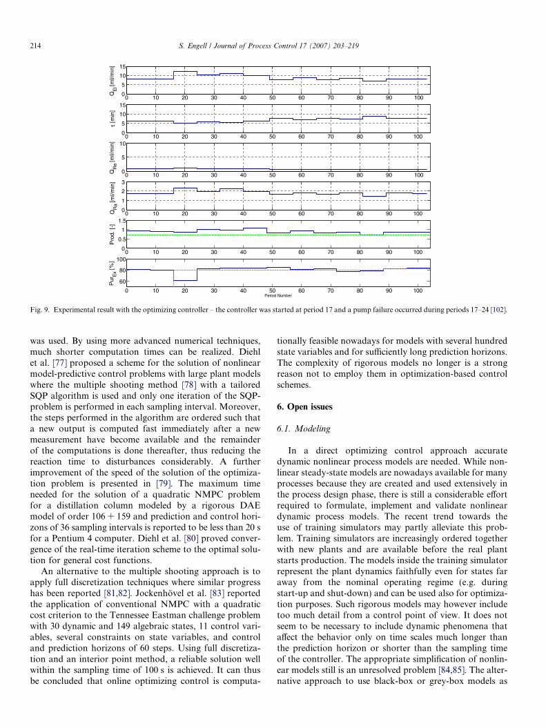
The performance of the controller is illustrated byFig. 7. The controller manages to track the purity referenceand to keep the productivity above its lower limits, while itimproves the economical operation of the plant by reduc-ing the solvent consumption. The optimizing controllerhas been implemented at a medium scale SMB plant usinga PLC-based process control system and an additional PCfor optimization and parameter estimation [102]. A photo-graph of the setup is shown in Fig. 8. The reactors are in aheated bath on top of the SMB plant. An experimentalresult where a significant disturbance – a pump failure –occurred exactly when the controller was switched on isshown in Fig. 9.

Fig. 8. Experimental SMB-plant with external reactors (in the heated bathon the top, left).

5.3. Numerical aspects

In the example described above, a relatively simplenumerical approach using direct simulation, computationof the gradients by perturbation and a feasible path SQPalgorithm for the computation of the optimal controls

0 50 100 150 200 250 300 350 400 4500

5

10

15

τ [m

in]

0 50 100 150 200 250 300 350 400 4500

5

10

15

QE

l [m

l/min

]

0 50 100 150 200 250 300 350 400 4500

5

10

QR

e [m

l/min

]

0 50 100 150 200 250 300 350 400 4500

1

2

3

QR

a [m

l/min

]

0 50 100 150 200 250 300 350 400 4500

0.5

1

1.5

Pro

d. [

-]

0 50 100 150 200 250 300 350 400 450

60

80

100

Pur

Ex [

%]

Period Number

Fig. 7. Simulation of the optimizing controller of the Hashimoto reactive SMB process. The controller was started at period 80. s denotes the switchingperiod, Prod the productivity. The dashed lines represent the set-points.

0 10 20 30 40 50 60 70 80 90 1000

5

10

15τ

[min

]

0 10 20 30 40 50 60 70 80 90 1000

5

10

15

QE

l [m

l/min

]

0 10 20 30 40 50 60 70 80 90 1000

5

10

QR

e [m

l/min

]

0 10 20 30 40 50 60 70 80 90 1000

1

2

3

QR

a [m

l/min

]

0 10 20 30 40 50 60 70 80 90 1000

0.5

1

1.5

Pro

d. [

-]

0 10 20 30 40 50 60 70 80 90 100

60

80

100

Pur

Ex [

%]

Period Number

Fig. 9. Experimental result with the optimizing controller – the controller was started at period 17 and a pump failure occurred during periods 17–24 [102].


was used. By using more advanced numerical techniques,much shorter computation times can be realized. Diehlet al. [77] proposed a scheme for the solution of nonlinearmodel-predictive control problems with large plant modelswhere the multiple shooting method [78] with a tailoredSQP algorithm is used and only one iteration of the SQP-problem is performed in each sampling interval. Moreover,the steps performed in the algorithm are ordered such thata new output is computed fast immediately after a newmeasurement have become available and the remainderof the computations is done thereafter, thus reducing thereaction time to disturbances considerably. A furtherimprovement of the speed of the solution of the optimiza-tion problem is presented in [79]. The maximum timeneeded for the solution of a quadratic NMPC problemfor a distillation column modeled by a rigorous DAEmodel of order 106 + 159 and prediction and control hori-zons of 36 sampling intervals is reported to be less than 20 sfor a Pentium 4 computer. Diehl et al. [80] proved conver-gence of the real-time iteration scheme to the optimal solu-tion for general cost functions.

An alternative to the multiple shooting approach is toapply full discretization techniques where similar progresshas been reported [81,82]. Jockenhovel et al. [83] reportedthe application of conventional NMPC with a quadraticcost criterion to the Tennessee Eastman challenge problemwith 30 dynamic and 149 algebraic states, 11 control vari-ables, several constraints on state variables, and controland prediction horizons of 60 steps. Using full discretiza-tion and an interior point method, a reliable solution wellwithin the sampling time of 100 s is achieved. It can thusbe concluded that online optimizing control is computa-

tionally feasible nowadays for models with several hundredstate variables and for sufficiently long prediction horizons.The complexity of rigorous models no longer is a strongreason not to employ them in optimization-based controlschemes.

6. Open issues

6.1. Modeling

In a direct optimizing control approach accuratedynamic nonlinear process models are needed. While non-linear steady-state models are nowadays available for manyprocesses because they are created and used extensively inthe process design phase, there is still a considerable effortrequired to formulate, implement and validate nonlineardynamic process models. The recent trend towards theuse of training simulators may partly alleviate this prob-lem. Training simulators are increasingly ordered togetherwith new plants and are available before the real plantstarts production. The models inside the training simulatorrepresent the plant dynamics faithfully even for states faraway from the nominal operating regime (e.g. duringstart-up and shut-down) and can be used also for optimiza-tion purposes. Such rigorous models may however includetoo much detail from a control point of view. It does notseem to be necessary to include dynamic phenomena thataffect the behavior only on time scales much longer thanthe prediction horizon or shorter than the sampling timeof the controller. The appropriate simplification of nonlin-ear models still is an unresolved problem [84,85]. The alter-native approach to use black-box or grey-box models as


proposed frequently in nonlinear model-predictive control[59,86–88] may be effective for regulatory control wherethe model only has to capture the essential dynamic fea-tures of the plant, but seems to be less suitable for optimiz-ing control where the optimal plant performance is aimedat and hence the best stationary values of the inputs andof the controlled variables have to be computed accuratelyby the controller.

6.2. Stability

Optimization of a cost function over a finite horizon ingeneral neither assures optimality of the complete trajec-tory beyond this horizon nor stability of the closed-loopsystem. Closed-loop stability has been addressed exten-sively in the theoretical research in nonlinear model-predic-tive control. The theoretical discussion has led to a clearunderstanding of what is required to ascertain the stabilityof a nonlinear model-predictive control scheme and clearlypointed out the deficiencies of less sophisticated schemes.Stability results so far have been proven for regulatoryNMPC where stability means convergence to the desiredequilibrium point. Stability can be assured by properchoice of the cost function within the prediction horizonand the addition of a cost on the terminal state and therestriction of the terminal state to a suitable set [89,90]. Ifthe cost function within the prediction horizon is an eco-nomic cost function, a bounded cost over the horizon willhowever in general not ensure boundedness of the devia-tion of the state vector from an equilibrium state becauseeconomic cost functions often involve only very few pro-cess variables, mostly input streams and mass flows leavingthe physical system. Moreover, in direct optimizing controlthere is no fixed equilibrium state.

A possible approach towards optimizing control withguaranteed stability is to compute the optimal steady stateonline first and then the optimal moves over the controlhorizon. In this case, the cost function can be extendedby a terminal cost that penalizes the distance of the stateat the end of the prediction horizon from the optimalsteady state and – if necessary by a (small) quadratic pen-alty term on the deviation of the state (or of suitable out-puts) from the terminal state within the predictionhorizon. If a suitable constraint on the terminal state isadded, this should provide a stabilizing control scheme.It has been demonstrated recently that algorithms of thistype are computationally feasible even for very large non-linear plant models [91]. By the choice of the weightingterms, a compromise can be established between optimiz-ing process performance over a limited horizon at a fastsampling rate and long-term performance under theassumption that no major disturbance occurs in the future.This leads to a hierarchical scheme similar to the RTO/MPC scheme where the upper layer provides the terminalstate and the terminal region and the lower layer now is‘‘cost-conscious’’ and no longer purely regulatory. In con-trast to the RTO/MPC-scheme, the optimization criteria as

well as the models used on both layers are consistent in thisstructure.

An alternative approach to guaranteeing stability of anoptimizing controller was applied in [51] to a linear processwith a static nonlinearity at the output, based on an aug-mented control Lyapunov function.

6.3. State estimation

For the computation of economically optimal processtrajectories based upon a rigorous nonlinear processmodel, the state variables of the process at the beginningof the prediction horizon must be known. As not all stateswill be measured in a practical application, state estimationis a key ingredient of a directly optimizing controller. Thestate estimation problem is of the same complexity as theoptimization problem, unless simple approaches as predict-ing the state by simulation of a process model areemployed. The natural approach is to formulate the stateestimation problem also as an optimization problem on amoving horizon [92–94]. The estimation of some importantbut variable or unknown model parameters can beincluded in this formulation. A control scheme whereNMPC is combined with moving horizon estimation hasrecently been realized in [95]. But still experience with theapplication of moving horizon state estimation is quite lim-ited to date. Simpler and computationally less demandingschemes as the constrained extended Kalman filter (CEKF)may provide a comparable performance and are more easyto implement (but not easier to tune) [48,96]. As accuratestate estimation is at least as critical for the performanceof the closed-loop system as the exact tuning of the opti-mizer, more attention should be paid to the investigationof the performance of state estimation schemes in realisticsituations with non-negligible model-plant mismatch.

6.4. Measurement-based optimization

In the scheme described in Section 5, feedback of themeasured variables is only realized via the updates of thestate and of the parameters and by a bias term in the for-mulation of the constraints and possibly in the cost crite-rion. As discussed in the Section on RTO, a near-optimalsolution requires that the gradients provided by the modeland the second derivatives are accurate. However in such ascheme there is no feedback present to establish optimalitydespite the presence of model errors. This can be addressedby the solution of a modified optimization problem [25,26]or by taking the presence of model errors into account inthe local search [28]. As shown by Tatjewski, [97], optimal-ity can be achieved in the presence of structural or para-metric plant-model mismatch even without parameterupdating by correcting the optimization criterion basedon gradient information derived from the available mea-surements. This idea was extended to handling constraintsand applied to batch chromatography in [98] and might beexplored in the continuous case as well. An alternative way


to implement measurement-based optimization is to for-mulate the optimization problem (partly) as the trackingof necessary conditions of optimality which are robustagainst model mismatch [99–101].

6.5. Reliability and transparency

As discussed above, relatively large nonlinear dynamicoptimization problems can nowadays be solved in real-time, so this issue does no longer prohibit the applicationof a direct optimizing control scheme to complex units. Apractically very important limiting issue however is thatof reliability and transparency. It is hard, if not impossibleto rule out that a nonlinear optimizer does not provide asolution which at least satisfies the constraints and givesa reasonable performance. While for RTO an inspectionof the commanded set-points by the operators usually willbe feasible, this is less likely in a dynamic situation. Henceautomatic result filters are necessary as well as a backupscheme that stabilizes the process in the case where theresult of the optimization is not considered safe. Butthe operators will still have to supervise the operation ofthe plant, so a control scheme with optimizing control mustbe structured into modules which are not too complex. Theconcept of adding a cost term that represents steady-stateoptimality as described above provides a possible solutionfor the dynamic online optimization of larger complexesbased on decentralized optimizing control of smaller units.The co-ordination of the units is performed by the steady-state real-time optimization that sends the desired terminalstates plus adequate penalty terms to the lower-level con-trols. These penalty terms must reflect the sensitivity ofthe global optimum with respect to local deviations, i.e.how an economic gain on the local level within the optimi-zation horizon is traded against a global loss due to notsteering the plant to the globally optimal steady state. Still,acceptance by the operators and plant managers will be amajor challenge. Good interfaces to the operators that dis-play the predicted moves and the predicted reaction of theplant and enable comparisons with their intuitive strategiesare believed to be essential for practical success.

6.6. Effort vs. performance

The gain in performance by a more sophisticated con-trol scheme always has to be traded against the increasein cost due to the complexity of the control scheme – acomplex scheme will not only cause cost for its implemen-tation but it will need more maintenance by better qualifiedpeople than a simple one. If a carefully chosen standardregulatory control layer leads to a close-to-optimal opera-tion, there is no need for optimizing control. If the distur-bances that affect profitability and cannot be handled wellby the regulatory layer (in terms of economic performance)are slow, the combination of regulatory control and RTOis sufficient. In a more dynamic situation or for complexnonlinear multivariable plants, the idea of direct optimiz-

ing control should be explored and implemented if signifi-cant gains can be realized in simulations. Similar to anyNMPC controller that is designed for reference tracking,a successful implementation will require careful engineeringsuch that as many uncertainties as possible are compen-sated by simple feedback controllers and only the keydynamic variables are handled by the optimizing controllerbased on a rigorous model of the essential dynamics and ofthe stationary relations of the plant without too muchdetail.

7. Conclusions

This survey paper points out that process control shouldbe seen as a means to optimize plant operations rather thanto just track pre-computed set-points. Appropriate selec-tion of the control structure and real-time optimization(RTO) provide significant contributions to plant profitabil-ity. Recent progress in numerical optimization algorithmsas well as in NMPC theory and technology has renderedthe application of online dynamic optimization based uponrigorous models to complex plants feasible. Using an eco-nomic cost function in the MPC computations instead ofa function that penalizes the distance to the desired set-points or trajectories which are assumed as given and fixedoffers new exiting possibilities. Several application studieshave already demonstrated the feasibility and the potentialof this approach. Industrial implementations will continueto require a considerable engineering effort in particularbecause of the issues of robustness and transparency. Thestructuring of a control system in hierarchical layers andsubsystems of reduced complexity will remain a key ingre-dient of solutions which are accepted in industrial practice,but the distribution of the functionalities between the lay-ers can be re-thought due to the possibilities of direct opti-mizing control.

Acknowledgements

The fruitful co-operation and discussions with MoritzDiehl, Karsten-Ulrich Klatt, Achim Kupper and AbdelazizToumi in the area of control of chromatographic separa-tions and in particular the efforts of the last two in the real-ization of the optimizing controller at a production-sizeplant in an university environment are very gratefullyacknowledged as well as the stimulating environment ofthe research unit (DFG-Forschergruppe) ‘‘IntegratedReaction and Separation Operations’’ at the Departmentof Biochemical and Chemical Engineering of UniversitatDortmund and the discussions within the co-operativeproject cluster (DFG-Paketantrag) ‘‘Optimization-basedcontrol of processing plants’’ comprising groups fromAachen, Dortmund, Heidelberg and Stuttgart. TheDeutsche Forschungsgemeinschaft provided essentialfinancial support in the context of these co-operativeresearch structures.


References

[1] M. Morari, G. Stephanopoulos, Y. Arkun, Studies in the synthesisof control structures for chemical processes, Part I, AIChE J. 26(1980) 220–232.

[2] L.T. Narraway, J.D. Perkins, G.W. Barton, Interaction betweenprocess design and process control: economic analysis of processdynamics, J. Process Control 1 (1991) 243–250.

[3] L.T. Narraway, J.D. Perkins, Selection of process control structurebased on linear dynamic economics, Ind. Eng. Chem. Res. 32 (1993)2681–2692.

[4] A. Zheng, R.V. Mahajannam, J.M. Douglas, Hierarchical procedurefor plantwide control system synthesis, AIchE J. 45 (1999) 1255–1265.

[5] S. Skogestad, Plantwide control: the search for the self-optimizingcontrol structure, J. Process Control 10 (2000) 487–507.

[6] T. Backx, O. Bosgra, W. Marquardt, Integration of model predictivecontrol and optimization of processes, in: Proceedings of IFACSymposium ADCHEM, Pisa, 2000, pp. 249–260.

[7] A.C. Zanin, M. Tvrzska de Gouvea, D. Odloak, Integrating real-time optimization into the model predictive controller of the FCCsystem, Contr. Eng. Pract. 10 (2002) 819–831.

[8] P.A. Rolandi, J.A. Romagnoli, A framework for online fulloptimizing control of chemical processes, in: Proceedings ofESCAPE 15, Elsevier, 2005, pp. 1315–1320.

[9] T.E. Marlin, A.N. Hrymak, Real-time operations optimization ofcontinuous processes, in: Proceedings of CPC V, AIChE SymposiumSeries, vol. 93, 1997, pp. 156–164.

[10] T. Larsson, K. Hestetun, E. Hovland, S. Skogestad, Self-optimizingcontrol of a large-scale plant: the Tennessee Eastman process, Ind.Eng. Chem. Res. 40 (2001) 4889–4901.

[11] T. Larsson, S. Govatsmark, S. Skogestad, Control structureselection for reactor, separator, and recycle processes, Ind. Eng.Chem. Res. 42 (2003) 1225–1234.

[12] S. Engell, T. Scharf, M. Volker, A methodology for control structureselection based on rigorous process models, in: 16th IFAC WorldCongress, Tu-E14-T0/6, 2005.

[13] J.J. Downs, E.F. Vogel, A plant-wide industrial process controlproblem, Comp. Chem. Eng. 17 (1993) 245–255.

[14] W. Findeisen, F.N. Bailey, M. Brdys, K. Malinowski, P. Wozniak,A. Wozniak, Control and Coordination in Hierarchical Systems,John Wiley, New York, 1980.

[15] I. Miletic, T.E. Marlin, Results analysis for real-time optimization(RTO): deciding when to change the plant operation, Comp. Chem.Eng. 20 (1996) 1077.

[16] C.V. Rao, J.B. Rawlings, Steady states and constraints in modelpredictive control, AIChE J. 45 (1999) 1266–1278.

[17] J.F. Forbes, T.E. Marlin, Design cost: a systematic approach totechnology selection for model-based real-time optimization sys-tems, Comp. Chem. Eng. 20 (1996) 717–734.

[18] Y. Zhang, J.F. Forbes, Extended design cost: a performancecriterion for real-time optimization systems, Comp. Chem. Eng. 24(2000) 1829–1841.

[19] I. Miletic, T.E. Marlin, On-line statistical results analysis in real-timeoperations optimization, Ind. Eng. Chem. Res. 37 (1998) 3670–3684.

[20] Y. Zhang, D. Nadler, J.F. Forbes, Results analysis for trustconstrained real-time optimization, J. Process Control 11 (2001)329–341.

[21] W.S. Yip, T.E. Marlin, The effect of model fidelity on real-timeoptimization performance, Comp. Chem. Eng. 28 (2004) 267–280.

[22] J.F. Forbes, T.E. Marlin, J. MacGregor, Model selection criteria foreconomics-based optimizing control, Comp. Chem. Eng. 18 (1994)497–510.

[23] J.F. Forbes, T.E. Marlin, Model accuracy for ecconomic optimizingcontrollers: the bias update case, Ind. Eng. Chem. Fund. 33 (1995)1919–1929.

[24] W.S. Yip, T.E. Marlin, Designing plant experiments for real-timeoptimization systems, Contr. Eng. Pract. 11 (2003) 837–845.

[25] P.D. Roberts, An algorithm for steady-state system optimizationand parameter estimation, Int. J. Syst. Sci. 10 (1979) 719–734.

[26] M. Brdys, J.E. Ellis, P.D. Roberts, Augmented integrated systemoptimization and parameter estimation technique: derivation, opti-mality and convergence, Proc. IEE 134 (1987) 201–209.

[27] H. Zhang, P.D. Roberts, On-line steady-state optimization ofnonlinear constrained processes with slow dynamics, Trans. Inst.Meas. Contr. 12 (1990) 251–261.

[28] J.H. Cheng, E. Zafiriou, Robust model-based iterative feedbackoptimization of steady-state plant operations, Ind. Eng. Chem. Res.39 (2000) 4215–4227.

[29] J. Zhou, A. Tits, C. Lawrence, User’s Guide for FFSQ, Version 3.7.,University of Maryland, 1997.

[30] P.M. Duvall, J.B. Riggs, On-line optimization of the TennesseeEastman challenge problem, J. Process Control 10 (2000) 19–33.

[31] E. Sequeira, M. Graells, L. Puigjaner, Real-time evolution of onlineoptimization of continuous processes, Ind. Eng. Chem. Res. 41(2002) 1815–1825.

[32] T. Jiang, B. Chen, X. He, P. Stuart, Application of steady-statedetection method based on wavelet transform, Comp. Chem. Eng.27 (2003) 569–578.

[33] K. Basak, K.S. Abhilash, S. Ganguly, D.N. Saraf, On-line optimi-zation of a crude distillation unit with constraints on productproperties, Ind. Eng. Chem. Res. 41 (2002) 1557–1568.

[34] J.S. Shamma, M. Athans, Gain scheduling: potential hazards andpossible remedies, IEEE Control Systems Magazine 12 (3) (1992)101–107.

[35] D.A. Lawrence, W.J. Rugh, Gain scheduling dynamic linearcontrollers for a nonlinear plant, Automatica 31 (1995) 381–390.

[36] A.M. Morshedi, C.R. Cutler, T.A. Skrovanek, Optimal solution ofdynamic matrix control with linear programming techniques, Proc.Am. Control Conf. 208 (1985).

[37] C. Brosilow, G.Q. Zhao, A linear programming approach toconstrained multivariable process control, Contr. Dyn. Syst. 27(1988) 14l.

[38] C. Yousfi, R. Tournier, Steady-state optimization inside modelpredictive control, Proc. Am. Control Conf. 1866 (1991).

[39] K.R. Muske, Steady-state target optimization in linear modelpredictive control, Proc. Am. Control Conf. 3597 (1997).

[40] R.C. Sorensen, C.R. Cutler, LP integrates economics into dynamicmatrix control, Hydrocarbon Process. 9 (1998) 57–65.

[41] R. Nath, Z. Alzein, On-line dynamic optimization of olefins plants,Comp. Chem. Eng. 24 (2000) 533–538.

[42] Ch. M. Jing, B. Joseph, Performance and stability analysis of LP-MPC and QP-MPC cascade control systems, AIChE J. 45 (7) (1999)1521–1534.

[43] A. Kassidas, J. Patry, T. Marlin, Integration of process andcontroller models for the design of self-optimizing control, Comp.Chem. Eng. 24 (2000) 2589–2602.

[44] A.C. Zanin, M. Tvrzska de Gouvea, D. Odloak, Industrial imple-mentation of a real-time optimization strategy for maximizingproduction of LPG in a FCC unit, Comp. Chem. Eng. 24 (2000)525–531.

[45] C.E.S. Costa, F.B. Freire, N.A. Correa, J.T. Freire, R.G. Correa,Two-layer real-time optimization of the drying of pastes in a spoutedbed: experimental implementation, in: 16th IFAC World Congress,Prague, 2005, Paper Fr-M06-TO/6.

[46] S.J. Qin, T. Badgewell, A survey of industrial model predictivecontrol technology, Contr. Eng. Pract. 11 (2003) 733–764.

[47] B.A. Foss, T.S. Schei, Putting nonlinear model predictive controlinto use. Preprints International Workshop on Assessment andFuture Directions of NMPC, Freudenstadt, 255–262.

[48] R.D. Bartusiak, NMPC: a platform for optimal control of feed- orproduct-flexible manufacturing, Preprints International Workshopon Assessment and Future Directions of NMPC, Freudenstadt,2005, pp. 3–14.

[49] K. Naidoo, J. Guiver, P. Turner, M. Keenan, M. Harmse,Experiences with nonlinear MPC in polymer manufacturing,


Preprints International Workshop on Assessment and FutureDirections of NMPC, Freudenstadt, 2005, pp. 335–345.

[50] A. Singh, J.F. Forbes, P.J. Vermeer, S.S. Woo, Model-based real-time optimization of automotive gasoline blending operations, J.Process Control 10 (2000) 43–58.

[51] T.A. Johansen, D. Sbarbaro, Lyapunov-based optimizing control ofnonlinear blending processes, IEEE Trans. Control Syst. Technol. 13(4) (2005) 631–638.

[52] J. Busch, M. Santos, J. Oldenburg, A. Cruse, W. Marquardt, Aframework for the mixed integer dynamic optimization ofwaste water treatment plants using scenario-dependent optimalcontrol, in: Proceedings of ESCAPE 15, Elsevier, 2005, pp.955–960.

[53] D. Broughton, C. Gerhold, Continuous sorption process employingfixed bed of sorbent and moving inlets and outlets, US Patent2985586, 1961.

[54] D.W. Guest, Evaluation of simulated moving bed chromatographyfor pharmaceutical process development, J. Chromatogr. A 760(1997) 159–162.

[55] M. Juza, M. Mazzotti, M. Morbidelli, Simulated moving-bedchromatography and its application to chirotechnology, TrendsBiotechnol. 18 (2000) 108–118.

[56] S. Engell, A. Toumi, Optimization and control of chromatography,Comp. Chem. Eng. 29 (2005) 1243–1252.

[57] A. Toumi, S. Engell, Advanced control of simulated moving bedprocesses, in: H. Schmidt-Traub (Ed.), Preparative Chromatogra-phy, Wiley-WCH, Weinheim, 2005, pp. 401–416 (Chapter 9).

[58] K.-U. Klatt, F. Hanisch, G. Dunnebier, S. Engell, Model-basedoptimization and control of chromatographic processes, J. ProcessControl 24 (2000) 1119–1126.

[59] C. Wang, K.-U. Klatt, G. Dunnebier, S. Engell, F. Hanisch, Neuralnetwork-based identification of SMB chromatographic processes,Contr. Eng. Pract. 11 (2003) 949–959.

[60] A. Toumi, S. Engell, Optimal operation and control of a reactivesimulated moving bed process, Preprints IFAC SymposiumADCHEM, Hong Kong, 2004, pp. 243–248.

[61] A. Toumi, S. Engell, Optimization-based control of a reactivesimulated moving bed process for glucose isomerization, Chem. Eng.Sci. 59 (2004) 3777–3792.

[62] A Toumi, M. Diehl, S. Engell, H.G. Bock, J.P. Schloder, Finitehorizon optimizing of control advanced SMB chromatographicprocesses, in: 16th IFAC World Congress, Fr-M06-TO/2, 2005.

[63] O. Ludemann-Hombourger, R.M. Nicoud, The VARlCOL process:a new multicolumn continuous separation process, Separat. Sci.Technol. 35 (2000) 1829–1862.

[64] A. Toumi, S. Engell, O. Ludemann-Hombourger, R.M. Nicoud, M.Bailly, Optimization of simulated moving bed and Varicol processes,J. Chromatogr. A 1006 (1–2) (2003) 15–31.

[65] M. Kearney, K. Hieb, Time variable simulated moving bed process,US Patent 5.102.553, 1992.

[66] G. Erdem, S. Abel, M. Morari, M. Mazzotti, M. Morbidelli,Automatic control of simulated moving beds. Part I: Linearisotherms, Ind. Eng. Chem. Res. 43 (2004) 405–421.

[67] G. Erdem, S. Abel, M. Morari, M. Mazzotti, M. Morbidelli,Automatic control of simulated moving beds. Part II: Nonlinearisotherms, Ind. Eng. Chem. Res. 43 (2004) 3895–3907.

[68] S. Abel, G. Erdem, M. Amanullah, M. Morari, M. Mazzotti, M.Morbidelli, Optimizing control of simulated moving beds-experi-mental implementation, J. Chromatogr. A 1092 (1) (2005) 2–16.

[69] S. Natarajan, J.H. Lee, Repetitive model predictive control appliedto a simulated moving bed chromatography system, Comp. Chem.Eng. 24 (2000) 1127–1133.

[70] T. Borren, J. Fricke, Chromatographic reactors, in: H. Schmidt-Traub (Ed.), Preparative Chromatography, Wiley-WCH, Weinheim,2005, pp. 371–400 (Chapter 8).

[71] T. Borren, J. Fricke, H. Schmidt-Traub, Reactive liquid chroma-tography, in: H. Schmidt-Traub, A. Gorak (Eds.), IntegratedReaction and Separation Operations, Springer, 2006 (Chapter 5).

[72] K. Hashimoto, S. Adachi, H. Noujima, Y. Ueda, A new processcombining adsorption and enzyme reaction for producing higher-fructose syrup, J. Biotechnol. Bioeng. 25 (1983) 2371–2393.

[73] A. Kupper, S. Engell, Nonlinear model predictive control of theHashimoto simulated moving bed process, in: International Work-shop on Assessment and Future Directions of NMPC, Freudenstadt,2005.

[74] A. Kupper, A. Toumi, S. Engell, Optimization and control ofreactive chromatographic processes, in: H. Schmidt-Traub, A.Gorak (Eds.), Integrated Reaction and Separation Operations,Springer, 2006, 2006 (Chapter 7).

[75] G. Guiochon, S. Golshan-Shirazi, A. Katti, Fundamentals ofPreparative and Nonlinear Chromatography, Academic Press,Boston, 1994.

[76] T. Gu, Mathematical Modelling and Scale Up of Liquid Chroma-tography, Springer, New York, 1995.

[77] M. Diehl, H.G. Bock, J.P. Schloder, Z. Nagy, F. Allgower, Real-time optimization and nonlinear model predictive control ofprocesses governed by differential-algebraic equations, J. Proc.Contr. 12 (2002) 577–585.

[78] H.G. Bock, K.J. Plitt, A multiple shooting algorithm for directsolution of optimal control problems, in: Proceedings of 9th IFACWorld Congress, Pergamon Press, Oxford, 1984, pp. 243–247.

[79] A. Schafer, P. Kuhl, M. Diehl, J.P. Schloder, H.G. Bock, Fastreduced multiple shooting methods for nonlinear model predictivecontrol, Chem. Eng. Process., submitted for publication.

[80] M. Diehl, H.G. Bock, J.P. Schloder, A real-time iteration scheme fornonlinear optimization in optimal feedback control, SIAM J.Control Optim. 43 (2005) 1714–1736.

[81] L.T. Biegler, A.M. Cervantes, A. Wachter, Advances in simulta-neous strategies for dynamic process optimization, Chem. Eng. Sci.57 (2002) 575–593.

[82] I.E. Grossmann, L.T. Biegler, Future perspective on optimization,Comp. Chem. Eng. 28 (2004) 1193–1218.

[83] T. Jockenhovel, L.T. Biegler, A. Wachter, Dynamic optimization ofthe Tennessee Eastman process using the OptControlCentre, Comp.Chem. Eng. 27 (2003) 1513–1531.

[84] J.H. Lee, Modeling and identification in nonlinear model predictivecontrol, in: F. Allgower, A. Zheng (Eds.), Nonlinear ModelPredictive Control, Birkhauser, 2000, pp. 269–293.

[85] W. Marquardt, Nonlinear model reduction for optimization basedcontrol of transient chemical processes, in: J.B. Rawlings, B.A.Ogunnaike, J.W. Eaton (Eds.), Proceedings of the 6th InternationalConference of Chemical Process Control, AIChE Symposium Series326, vol. 98, 2002, pp. 12–42.

[86] A. Draeger, S. Engell, Nonlinear model predictive control usingneural net plant models, in: R. Berber (Ed.), Methods of Model BasedProcess Control, Kluwer Academic Publishers, 1995, pp. 627–639.

[87] B.A. Foss, T.A. Johansen, A.V. Sorensen, Nonlinear predictivecontrol using local models – applied to a batch process, Control Eng.Practice 3 (1995) 389–396.

[88] E.F. Camacho, C. Bordons, Nonlinear model predictive control: anintroductory survey, Preprints International Workshop on Assess-ment and Future Directions of NMPC, Freudenstadt, 2005, pp. 15–30.

[89] H. Chen, F. Allgower, A quasi-infinite horizon nonlinear modelpredictive control scheme with guaranteed stability, Automatica 14(1998) 1205–1217.

[90] D.Q. Mayne, J.B. Rawlings, C.V. Rao, P.O.M. Scokaert, Con-strained model predictive control: stability and optimality, Autom-atica 36 (2000) 789–814.

[91] R. Roman, Z.K. Nagy, F. Allgower, S.P. Agachi, Dynamicmodeling and nonlinear model predictive control of a fluid catalyticcracking unit, in: Proceedings of ESCAPE 15, Elsevier, 2005, pp.1363–1368.

[92] S.-S. Jang, B. Joseph, H. Mukai, Comparison of two approaches toonline parameter and state estimation of nonlinear systems, Ind.Eng. Chem. Proc. Des. Develop. 25 (1986) 809–814.


[93] K.R. Muske, J.B. Rawlings, Nonlinear moving horizon stateestimation, in: R. Berber (Ed.), Methods of Model Based ProcessControl, Kluwer Academic Publishers, 1995, pp. 349–365.

[94] C.V. Rao, J.B. Rawlings, D.Q. Mayne, Constrained state estimationfor nonlinear discrete-time systems, IEEE Trans. AC 48 (2003) 246–258.

[95] M. Diehl, P. Kuhl, H.G. Bock, J.P. Schloder, B. Mahn, J. Kallrath,Combined nonlinear model predictive control and moving horizonestimation for a copolymerization process, in: Proc. ESCAPE 16/PSE 2006, Computer-Aided Chemical Engineering, vol. 21B, Else-vier, 2006, pp. 1527–1532.

[96] R. Gesthuisen, K.-U. Klatt, S. Engell, Optimization-based stateestimation – a comparative study fort the batch polycondensation ofPET, in: Proceedings of ECC 2001 Porto, 2001, pp. 1062–1067.

[97] P. Tatjewski, Iterative optimizing set-point control – the basicprinciple redesigned, in: 15th IFAC World Congress, Barcelona,2002, Paper T-Th-E16-3.

[98] W. Gao, S. Engell, Iterative set-point optimisation of batchchromatography, Comp. Chem. Eng. 29 (2005) 1401–1410.

[99] B. Srinivasan, D. Bonvin, E. Visser, S. Palanki, Dynamic optimi-zation of batch processes II. Role of measurements in handlinguncertainty, Comp. Chem. Eng. 27 (2002) 27–44.

[100] C. Chatzidoukas, C. Kiparissides, B. Srinivasan, D. Bonvin,Optimisation of grade transitions in an industrial gas-phaseolefin polymerization fluidized bed reactor via NCO tracking, in:16th IFAC World Congress, Prague, 2005, Paper Mo-A06-TO/2.

[101] J.V. Kadam, M. Schlegel, B. Srinivasan, D. Bonvin, W. Marquardt,Dynamic real-time optimization: from off-line numerical solution tomeasurement-based implementation. in: 16th IFAC World Con-gress, Prague, 2005, Paper Fr-M06-TO/1.

[102] A. Kupper, S. Engell, Optimizing control of the Hashimoto SMBprocess: experimental application, in: IFAC Symposium DYCOPS2007, submitted for publication.

feedback control for optimal process operation · feedback control for optimal process operation...

Documents