FEM and BEM simulations with the Gypsilab

framework

Francois Alouges∗and Matthieu Aussal†

Abstract

Gypsilab is a Matlab toolbox which aims at simplifying the devel-opment of numerical methods that apply to the resolution of problemsin multiphysics, in particular, those involving FEM or BEM simulations.The specifities of the toolbox, in particular its ease of use, are showntogether with the methodology we have followed for its development.Example codes that are short though representative enough are givenboth for FEM and BEM applications. A performance comparison withFreeFem++ is also provided.

1 Introduction

The finite element method (FEM) is nowadays extremely developed and hasbeen widely used in the numerical simulation of problems in continuum me-chanics, both for linear and non-linear problems. Many softwares exist amongwhich we may quote free ones (e.g. FreeFem++ [8], FENICS [12], FireDrake[13], Xlife++ [11], Feel++ [9], GetDP [14, 15], etc.) or commercial ones (e.g.COMSOL [16]). The preceding list is far from being exhaustive as the methodhas known many developments and improvements and is still under active studyand use. Numerically speaking, and without entering into too much details, letus say that the peculiarity of the method is that it is based on a variational for-mulation that leads to sparse matrices the size of which is typically proportionalto the number of unknowns. Direct or iterative methods can then be used tosolve the underlying linear systems.

On the other hand, the boundary element method (BEM) is used for prob-lems which can be expressed using a Green kernel. A priori restricted to linearproblems, the method inherently possesses the faculty of handling free spacesolutions and is therefore currently used for solving Laplace equations, wavescattering (in acoustics, electromagnetics or elastodynamics), or Stokes equa-tions for instance. Although it leads to dense matrices, which storage is pro-portional to the square of the number of unknowns, the formulation is usually

∗CMAP - Ecole Polytechnique, Universite Paris-Saclay, Route de Saclay, 91128, PalaiseauCedex, France. francois.alouges@polytechnique.edu .†CMAP - Ecole Polytechnique, Universite Paris-Saclay, Route de Saclay, 91128, Palaiseau

Cedex, France. matthieu.aussal@polytechnique.edu .

1

restricted to the boundary of the domain under consideration (e.g. the scat-terer), which lowers the dimension of the object that needs to be discretized.Nevertheless, due to computer limitations, those methods may require a specialcompression technique such as the Fast Multipole Method (FMM) [5, 7], theH-matrix storage [6] or the more recent Sparse Cardinal Sine Decomposition[1, 2, 3], in order to be applied to problems of sizes relevant for an accuratesimulation. In terms of softwares available for the simulation with this kind ofmethods, and probably due to the technicality sketched above, the list is muchshorter than before. In the field of academic, freely available softwares, one canquote BEM++ [10], or Xlife++ [11]. Commercial softwares using the methodare for instance the ones distributed by ESI Group (VAone for acoustics [25]and E-Field [26] for electromagnetism), or Aseris [27]. Again, the preceding listis certainly not exhaustive.

Eventually, one can couple both methods, in particular to simulate multi-physics problems that involve different materials and for which none of the twomethods apply directly. This increases again the complexity of the methodologyas the user needs to solve coupled equations that are piecewise composed of ma-trices sparsely stored combined with other terms that contain dense operatorsor compressed ones. How to express such a problem? Which format should beused for the matrix storage? Which solver applies to such cases, an iterative ora direct one? Eventually, the writing of the software still requires abilities thatmight be out of his/her field of expertise.

As a sake of example, it is very important to notice that, to the knowledgeof the authors, the only freely available software, which uses the BEM, and forwhich the way of programming is comparable to FreeFem++, is BEM++ thathas been interfaced into FENICS.

The preceding considerations have led us to develop the toolbox openFEMwhich aims at simplifying and generalizing the development of FEM-BEM cou-pling simulation algorithms and methods. Written as a full Matlab suite ofroutines, the toolbox can be used to describe and solve various problems thatinvolve FEM and/or BEM techniques. We have also tried to make the finiteelement programming as simple as possible, using a syntax comparable to theone used in FreeFem++ or FENICS/FireDrake and very close to the mathe-matical formulation itself which is used to discretize the problems. The toolboxis a part of a more general environment, called Gypsilab, that contains severaltoolboxes:

• openMSH for the handling of meshes;

• openDOM for the manipulation of quadrature formulas;

• openHMX that contains the full H-matrix algebra [6], including the LUfactorization and inversion;

• openFEM for the finite element and boundary element methods.

Other toolboxes are also developed inside Gypsilab that we plan to describeelsewhere.

2

Eventually, although the main goal is not the performance, the toolboxopenFEM may handle, on classical computers, problems whose size reachesa few millions of unknowns for the FEM part and a few hundreds of thousandsof unknowns for the BEM when one uses compression. For FEM applications,this performance is very much comparable to already proposed Matlab strate-gies [22, 23, 24], though with much higher generality and flexibility.

The present paper explains in some details the capabilities of the toolboxopenFEM together with its use. Explanations concerning the implementationare also provided that give insight of the genericity of the approach. In orderto simplify the exposition, we focus here on FEM or BEM applications, leavingcoupled problems to a forthcoming paper.

Due to its simplicity of use, we strongly believe that the software describedhere could become a reference in the field. Indeed, applied mathematicians,interested in developing new FEM-BEM coupled algorithms need such tools inorder to address problems of significant sizes for real applications. Moreover, thesoftware is also ideal for the prototyping of academic or industrial applications.

2 Simple examples

We show in this Section a series of small example problems and correspondingMatlab listings.

2.1 A Laplace problem with Neumann boundary condi-tions

Let us start with the writing of a finite element program that solves the partialdifferential equation (PDE) −∆u+ u = f on Ω ,

∂u

∂n= 0 on ∂Ω ,

(1)

where the right-hand side function f belongs to L2(Ω). Here Ω stands for adomain in R2 or R3.

The variational formulation of this problem is very classical and reads:

Find u ∈ H1(Ω) such that ∀v ∈ H1(Ω)∫Ω

∇v(x) · ∇u(x) dx+

∫Ω

v(x)u(x) dx =

∫Ω

f(x)v(x) dx .

The finite element discretization is also straightforward and requires solvingthe same variational formulation where H1(Ω) is replaced by one of its finitedimensional subspaces (for instance the set of continuous and piecewise affineon a triangular mesh of Ω in the case of linear P 1 elements).

3

We give hereafter the openFEM source code used to solve such a problemin the case where the domain under consideration is the unit disk in R2, andthe function f is given by f(x, y, z) = x2.

1 % Library paths2 addpath ( ' . . / openDom ' )3 addpath ( ' . . / openMsh ' )4 addpath ( ' . . / openFem ' )5 % Mesh o f the d i sk6 N = 1000 ;7 mesh = mshDisk (N, 1 ) ;8 % I n t e g r a t i o n domain9 Omega = dom(mesh , 3 ) ;

10 % F i n i t e e lements11 Vh = fem (mesh , 'P1 ' ) ;12 % Matrix and RHS13 f = @(X) X( : , 1 ) . ˆ 2 ;14 K = i n t e g r a l (Omega , grad (Vh) , grad (Vh) ) + i n t e g r a l (Omega ,Vh,Vh) ;15 F = i n t e g r a l (Omega , Vh, f ) ;16 % So lv ing17 uh = K \ F;18 f i g u r e19 graph (Vh, uh) ;

We believe that the listing is very clear and almost self explanatory. Besidesinitialization (lines 2-4), one recognizes the meshing part in which a disk ismeshed with 1000 vertices (lines 6-7), the definition of an integration domain(line 9), the finite element space (line 11), the variational formulation of theproblem (lines 13-15) and the resolution (lines 17). Let us immediately insiston the fact that the operators constructed by the integral keyword are reallymatrices and vectors Matlab objects so that one can use classical Matlabfunctionalities for the resolution (here the backslash operator \). Ploting thesolution (lines 20-21) leads to the figure reported in Fig. 1.

2.2 Fourier boundary conditions

We now consider the problem −∆u+ u = 0 on Ω ,∂u

∂n+ u = g on ∂Ω ,

(2)

Again, the variational formulation of the problem is standard and reads asfollows

Find u ∈ H1(Ω) such that ∀v ∈ H1(Ω)∫Ω

∇v(x) · ∇u(x) dx+

∫Ω

v(x)u(x) dx+

∫∂Ω

v(s)u(s) ds =

∫∂Ω

g(s)v(s) ds .

4

Figure 1: Numerical solution of (1) on a unit disk using Gypsilab.

The preceding code is modified in the following way (we have taken theexample where g(s) = 1).

1 % Library paths2 addpath ( ' . . / openDom ' )3 addpath ( ' . . / openMsh ' )4 addpath ( ' . . / openFem ' )5 % Create mesh d i sk + boundary6 N = 1000 ;7 mesh = mshDisk (N, 1 ) ;8 meshb = mesh . bnd ;9 % I n t e g r a t i o n domains

10 Omega = dom(mesh , 7 ) ;11 Sigma = dom(meshb , 3 ) ;12 % F i n i t e element space13 Vh = fem (mesh , 'P2 ' ) ;14 % Matrix and RHS15 K = i n t e g r a l (Omega , grad (Vh) , grad (Vh) ) ...16 + i n t e g r a l (Omega , Vh, Vh) ...17 + i n t e g r a l ( Sigma , Vh, Vh) ;18 g = @(x ) ones ( s i z e (x , 1 ) ,1 ) ;19 F = i n t e g r a l ( Sigma , Vh, g ) ;20 % Reso lut ion21 uh = K \ F;22 f i g u r e23 graph (Vh, uh) ;

Compared to the preceding example, a boundary mesh and an associatedintegration domain are also defined (lines 8 and 11). Let us note the piecewisequadratic (so-called P 2) element used (line 13) which leads to use more accurate

5

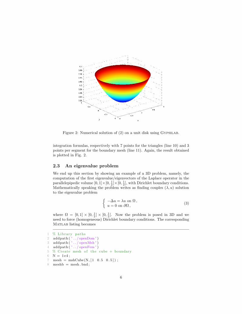
Figure 2: Numerical solution of (2) on a unit disk using Gypsilab.

integration formulas, respectively with 7 points for the triangles (line 10) and 3points per segment for the boundary mesh (line 11). Again, the result obtainedis plotted in Fig. 2.

2.3 An eigenvalue problem

We end up this section by showing an example of a 3D problem, namely, thecomputation of the first eigenvalue/eigenvectors of the Laplace operator in theparallelepipedic volume [0, 1]×[0, 1

2 ]×[0, 12 ], with Dirichlet boundary conditions.

Mathematically speaking the problem writes as finding couples (λ, u) solutionto the eigenvalue problem

−∆u = λu on Ω ,u = 0 on ∂Ω ,

(3)

where Ω = [0, 1] × [0, 12 ] × [0, 1

2 ]. Now the problem is posed in 3D and weneed to force (homogeneous) Dirichlet boundary conditions. The correspondingMatlab listing becomes

1 % Library paths2 addpath ( ' . . / openDom ' )3 addpath ( ' . . / openMsh ' )4 addpath ( ' . . / openFem ' )5 % Create mesh o f the cube + boundary6 N = 1e4 ;7 mesh = mshCube(N, [ 1 0 .5 0 . 5 ] ) ;8 meshb = mesh . bnd ;

6

9 % I n t e g r a t i o n domains10 Omega = dom(mesh , 4 ) ;11 % F i n i t e element space12 Vh = fem (mesh , 'P1 ' ) ;13 Vh = d i r i c h l e t (Vh, meshb ) ;14 % Matrix and RHS15 K = i n t e g r a l (Omega , grad (Vh) , grad (Vh) ) ;16 M = i n t e g r a l (Omega , Vh, Vh) ;17 % Reso lut ion18 Neig = 10 ;19 [V,EV] = e i g s (K,M, Neig , 'SM ' ) ;

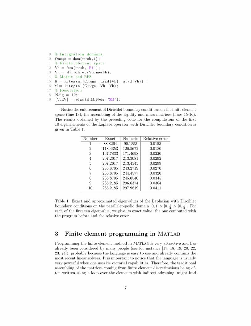
Notice the enforcement of Dirichlet boundary conditions on the finite elementspace (line 13), the assembling of the rigidity and mass matrices (lines 15-16).The results obtained by the preceding code for the computatoin of the first10 eigenelements of the Laplace operator with Dirichlet boundary condition isgiven in Table 1.

Number Exact Numeric Relative error1 88.8264 90.1853 0.01532 118.4353 120.5672 0.01803 167.7833 171.4698 0.02204 207.2617 213.3081 0.02925 207.2617 213.4545 0.02996 236.8705 243.2719 0.02707 236.8705 244.4577 0.03208 236.8705 245.0540 0.03459 286.2185 296.6374 0.036410 286.2185 297.9819 0.0411

Table 1: Exact and approximated eigenvalues of the Laplacian with Dircihletboundary conditions on the parallelepipedic domain [0, 1] × [0, 1

2 ] × [0, 12 ]. For

each of the first ten eigenvalue, we give its exact value, the one computed withthe program before and the relative error.

3 Finite element programming in Matlab

Programming the finite element method in Matlab is very attractive and hasalready been considered by many people (see for instance [17, 18, 19, 20, 22,23, 24]), probably because the language is easy to use and already contains themost recent linear solvers. It is important to notice that the language is usuallyvery powerful when one uses its vectorial capabilities. Therefore, the traditionalassembling of the matrices coming from finite element discretizations being of-ten written using a loop over the elements with indirect adressing, might lead

7

to prohibitive execution times in Matlab. This problem was identified a longtime ago and several ways have already been proposed to circumvent it. Inparticular, in [22], are given and compared different alternatives that lead tovery efficient assembling. Many languages are also compared (C++, Matlab,Python, FreeFem++), and it is shown that the C++ implementation onlybrings a slight improvement in performance. Other Matlab implementationsare proposed in the literature (see e.g. [17, 19, 20, 23, 24]), but they all sufferfrom the lack of generality. The problem solved is indeed very often the Lapla-cian with piecewise linear finite elements and one needs to adapt the approachfor any different problem.

We have followed yet another strategy that has the great advantage to bevery general and easily adaptable to a wide variety of possible operators tobuild and solve, and which also enables the user to assemble matrices that comefrom the coupling between different finite elements. Moreover, we will see thatthe method also leads to reasonably good assembling times. To this aim, wegive the following example from which one can understand the generality of theapproach and the way openFEM is coded.

Let us consider the case of assembling the mass matrix. To be more precise,we call T a conformal triangulation1 on which one has to compute the matrixA whose entries are given by

Aij =

∫Tφi(x)φj(x) dx . (4)

Here we have used the notation (φi)1≤i≤N to denote the basis functionsof the finite element (discrete) space of dimension N . To gain generality, thepreceding integral is usually not computed exactly, but rather approximatedusing a quadrature rule. Thus, calling (xk, ωk)1≤k≤M the set of all quadraturepoints over T , we write

Aij ∼M∑k=1

ωkφi(xk)φj(xk) . (5)

Introducing now the two matrices W and C (respectively of size M×M andM ×N) defined by

Wkk = ωk for 1 ≤ k ≤M , and Bkj = φj(xk) for 1 ≤ k ≤M, 1 ≤ j ≤ N , (6)

we may rewrite (5) asA ∼ BtW B , (7)

the approximation coming from the fact that a quadrature rule has been usedinstead of an exact formula. In particular, we notice that if the quadratureformula is exact in (5), then the approximation is in fact an equality.

From the preceding considerations the procedure that enables to assemblethe sparse mass matrix can be summarized as:

1Triangulation usually means a 2D problem, while we would have to consider a tetrahedralmesh for 3D problems. This is not a restriction as we can see.

8

• Knowing the triangulation (resp. tetrahedral mesh), and a quadrature for-mula on a reference triangle (resp. tetrahedron), build the set of quadra-ture points/weights (xk, ωk)1≤k≤M .

• Knowing the finite element used (or, equivalently, the basis functions(φj)1≤j≤N ) and the quadrature points (xk)1≤k≤M , build the matrices Wand B.

• Eventually, compute A = BtW B .

Notice that the matrices W and B are usually sparse. Indeed, W is actuallydiagonal, while B has a non zero entry Bjk only for the quadrature points xkthat belong to the support of φj . In terms of practical implementation, thematrix W is assembled using a spdiags command while the matrix B is builtusing a vectorized technique.

The preceding procedure is very general and does only rely on the chosenfinite element or the quadrature formula. Moreover, the case of more compli-cated operators can also be treated with only slight modifications. Indeed, ifone considers the case of the Laplace operator, for which the so-called rigiditymatrix is given by

Kij =

∫T∇φi(x) · ∇φj(x) dx , (8)

one may write similarly

Kij ∼M∑k=1

ωk∇φi(xk) · ∇φj(xk) , (9)

from which one deduces

K ∼ CtxW Cx + Ct

yW Cy + CtzW Cz ,

where the matrix W is the same than before and the matrices Cx, Cy and Cz

are given for 1 ≤ k ≤M, 1 ≤ j ≤ N by

Cx,kj =∂φj∂x

(xk) , Cy,kj =∂φj∂y

(xk) , Cz,kj =∂φj∂z

(xk) . (10)

In openFEM all those matrices are built “on the fly” upon request of theuser of the desired final matrix. This might slow down a bit the method to thebenefit of a very little footprint in memory and much higher genericity.

4 Quick overview of openFEM

This section is not intended to be a user’s manual. We just give the mainfunctionalities of openFEM and refer the interested reader to the website [28].openFEM follows the programming principles of the whole environment Gyp-silab which tries to compute as much as possible the quantities “on the fly”,

9

or in other words, to keep in memory as little information as possible. Themain underlying idea is that storing many matrices (even sparse) might becomememory consuming, and recomputing on demand the corresponding quantitiesdoes not turn to be the most costly part in usual computations. Having thisidea in mind helps in understanding all the “philosophy” that we have followedfor the development of the different toolboxes. Moreover, the whole library isobject oriented and the toolboxes have been implemented as value classes.

4.1 The mesh and the integration domain

openFEM is built in strong interaction with the toolboxes openMSH andopenDOM which are respectively devoted to handle meshes ans quadratureformula. Namely, we distinguish between two geometrical objects:

• The mesh. It is a purely geometric object with which one can computeonly geometric quantities (e.g. normals, volumes, edges, faces, etc.). Amesh can be of dimension 1 (a curve), 2 (a surface) or 3 (a volume) butis always embedded in the dimension 3 space and is a simplicial mesh(i.e. composed of segments, triangles or tetrahedra). It is defined by threetables :

– A list of vertices, which is a table of size Nv × 3 containing the threedimensional coordinates of the vertices ;

– A list of elements, which is a table of size Ne × (d + 1), d being thedimension of the mesh and Ne the number of elements ;

– A list of colours, which is a column vector of size Ne × 1 defining acolour for each element of the mesh, this last table being optional.

A typical msh object is given by the following structure.

>>mesh

mesh =

2050x3 msh array with properties:

vtx: [1083x3 double]

elt: [2050x3 double]

col: [2050x1 double]

The openMSH toolbox does not yet contain a general mesh generator perse. Only simple objects (cube, square, disk, sphere, etc.) can be meshed.More general object may be nevertheless loaded using classical formats(.ply, .msh, .vtk, .stl, etc.). Since the expected structure for a mesh isvery simple, the user may also his/her own wrapper to create the abovetables.

10

Any operation on meshes (e.g. intersection or union of different meshes,extraction of the boundary, etc.) is coded inside the openMSH toolbox.Let us emphasize that upon loading, meshes are automatically cleaned byremoving unnecessary or redondant vertices or elements.

• The domain which is a geometric object on which one can furthermoreintegrate. Numerically speaking, this is the concatenation of a mesh anda quadrature formula, identified by a number, that one uses with the cor-responding simplices of the mesh, in order to integrate functions. Thedefault choice is a quadrature formula with only one integration point lo-cated at the center of mass of the simplices.This is usually very inaccurate,and this is almost always mandatory to enhance the integration by takinga higher degree quadrature formula. A domain is defined using the dom

keyword. For instance, the command

1 Omega = dom(mesh ,4);

defines an integration domain Omega from the mesh, using an integrationformula with 4 integration points. If such an integration formula is notavailable, the program returns an error. Otherwise, the command createsan integration domain with the structure shown by the following output.

>> omega = dom(mesh,4)

omega =

dom with properties:

gss: 4

msh: [2050x3 msh]

We believe that making the construction of the quadrature formula veryexplicit helps the user to pay attention to this very important point, andmake the right choice for his/her application. In particular, for finiteelement computing, the right quadrature formula that one needs to usedepends on the order of the chosen finite element. Integration functional-ities are implemented in the openDOM toolbox (see below).

4.2 The Finite Element toolbox (openFEM)

Finite element spaces are defined through the use of the class constructor fem.Namely, the command

1 Vh = fem(mesh , name);

creates a finite element space on the mesh (an arbitrary 2D or 3D mesh definedin R3) of type defined by name. At the moment of the writing of this paper 3different families of finite elements are available:

11

• The Lagrange finite elements. The orders 0, 1 and 2 are only availablefor the moment. They corresponds to piecewise polynomials of degree 0,1 and 2 respectively. They are available in 2D or 3D.

• The edge Nedelec finite element. It is a space of vectorial functions whosedegrees of freedom are the circulation along all the edges of the underlyingmesh. This finite element is defined in both 2D and 3D. In 2D is imple-mented a general form for which the underlying surface does not need tobe flat.

• The Raviart-Thomas, also called Rao-Wilton-Glisson (RWG) finite ele-ments. Also vectorial, the degrees of freedom are the fluxes through theedges (in 2D) or the faces (in 3D) of the mesh. Again, the 2D implemen-tation is available for general non-flat surfaces.

For the two last families, only the lowest orders are available. The value of thevariable name should be one of ’P0’, ’P1’, ’P2’, ’NED’, ’RWG’ respectively,depending on the desired finite element in the preceding list.

Besides the definition of the finite element spaces, the toolbox openFEMcontains a few more functionalities, as the following.

• Operators. Operators can be specified on the finite element space itself.Indeed, we have already seen the example

1 A = integral(dom , grad(Vh), grad(Wh));

which returns the matrix of the Laplacian. Available operators are:

– grad, div, curl, which are differential operators that act on scalaror vectorial finite elements.

– curl, div, nxgrad, divnx, ntimes. Those operators are definedwhen solving problems on a bidimensional surface in R3. Here n

stands for the (outer) normal to the surface and all the differentialoperators are surfacic. Such operators are commonly used when solv-ing problems with the BEM (see below).

• Plots. Basic functions to plot a finite element or a solution are available.Namely, we have introduced

1 plot(Vh);

where Vh is a finite element space to plot the degrees of freedom the defineits functions, and

1 surf(Vh ,u);

in order to plot a solution. In that case the figure produced consists in thegeometry on which the finite element is defined coloured by the magnitudeof the u. Eventually, as we have seen in the first examples presented in thispaper, the command graph plots the graph of a finite element computedon a 2D flat surface.

12

1 graph(Vh ,u);

4.3 The integral keyword (openDOM)

Every integration done on a domain is evaluated through the keyword integral.Depending on the context explained below, the returned value can be either anumber, a vector or a matrix. More precisely, among the possible syntaxes are

• I = integral(dom, f);

where dom is an integration domain on which the integral of the functionf needs to be computed. In that case the function f should be defined ina vectorial way, depending on a variable X which can be a N × 3 matrix.For instance the definitions

1 f = @(X) X(:,1).*X(:,2);

2 g = @(X) X(:,1).^2 + X(:,2).^2 + X(:,3) .^2;

3 h = @(X) X(:,1) + X(:,2).*X(:,3);

respectively stand for the (3 dimensional) functions

f(x, y, z) = xy , g(x, y, z) = x2 + y2 + z2 , h(x, y, z) = x+ yz .

Since domains are all 3 dimensional (or more precisely embedded in the 3dimensional space), only functions of 3 variables are allowed.

• I = integral(dom, f, Vh);

In that case, f is still a 3 dimensional function as before while Vh standsfor a finite element space. The returned value I is a column vector whoseentries are given by

Ii =

∫dom

f(X)φi(X) dX

for all basis function φi of the finite element space.

• I = integral(dom, Vh, f);

This case is identical to the previous one but now, the returned vector isa row vector.

• A = integral(dom, Vh, Wh);

where both Vh and Wh are finite element spaces. This returns the matrixA defined by

Aij =

∫dom

φi(X)ψj(X) dX

where φi (resp. ψj) stands for the current basis function of Vh (resp. Wh).

• A = integral(dom, Vh, f, Wh);

This is a simple variant where the entries of the matrix A are now givenby

Aij =

∫dom

f(X)φi(X)ψj(X) dX .

13

As a matter of fact, the leftmost occuring finite element space is assumed tocorrespond to test functions while the rightmost one to the unknowns.

5 Generalization of the approach to the BEM

It turns out that the preceding approach, described in section 3, can be gen-eralized to the Boundary Element Method (BEM). In such contexts, after dis-cretization, one has to solve a linear system where the underlying matrix is fullypopulated. Typical examples are given by the acoustic or electromagnetic scat-tering. Indeed, let us consider a kernel2 G(x, y) for which one has to computethe matrix A defined by the entries

Aij =

∫x∈Σ1

∫y∈Σ2

φi(x)G(x, y)ψj(y) dx dy . (11)

This is very typical when one implements the BEM with a Galerkin approxi-mation, the functions (φi)1≤i≤N1 and (ψj)1≤j≤N2 , being basis functions of pos-sibly different finite element spaces. Taking discrete integration formulas on Σ1

and Σ2 respectively defined by the points and weights (xk, ωk)1≤k≤Nint1and

(yl, ηl)1≤l≤Nint2, leads to the approximation

Aij ∼∑k

∑l

φi(xk)ωkG(xk, yl)ηlψj(yl) , (12)

which enables us to write in a matrix form

A ∼ ΦWxGWyΨ . (13)

In this formula, the matricesWx andWy are the diagonal sparse matrices definedas before in (6) which depend on the quadrature weights ωk and ηl respectively.The matrices Φ and Ψ are the (usually sparse) matrices defined as in (7) forthe basis functions φi and ψj respectively, and G is the dense matrix of sizeNint1 ×Nint2 given by Gkl = G(xk, yl).

Again, building the sparse matrices as before, one only needs to furthercompute the dense matrix G and assemble the preceding matrix A with onlymatrix products.

5.1 Generalization of the integral keyword (openDOM)

In terms of the syntax, we have extended the range of the integral keywordin order to handle such integrals. Indeed, the preceding formulas show thatthere are very little differences with respect to the preceding FEM formulations.Namely, we now need to handle

• Integrations over 2 possibly different domains Σ1 and Σ2;

2For instance, in the case of acoustic scattering, G is the Helmholtz kernel defined by

G(x, y) =exp(ik|x−y|)

4π|x−y| .

14

• Any kernel depending on two variables provided by the user;

• As before, two finite element spaces that are evaluated respectively on xand y.

Furthermore, other formulations exist for the BEM, such as the so-called collo-cation method, in which one of the two integrals is replaced by an evaluation ata given set of points. This case is also very much used when one computes (seethe section below) the radiation of a computed solution on a given set of points.

To handle all these situations three possible cases are provided to the user:

• The case with two integrations and two finite element spaces. This corre-sponds to computing the matrix

Aij =

∫x∈Σ1

∫y∈Σ2

φi(x)G(x, y)ψj(y) dx dy ,

and is simply performed in Gypsilab by the following command.

1 A = integral(Sigma1 , Sigma2 , Phi , G, Psi);

As before, the first finite element space Phi is considered as the test-function space while the second one, Psi, stands for the unknown. Thetwo domains on which the integrations are performed are given in the sameorder than the finite element spaces (i.e. Phi and Psi are respectivelydefined on Σ1 and Σ2).

• The cases with only one integration and one finite element space. Twopossibilities fall in this category. Namely the computation of the matrix

Bij =

∫x∈Σ1

φi(x)G(x, yj) dx ,

for a collection of points yj and the computation of the matrix

Cij =

∫y∈Σ2

G(xi, y)ψj(y) dy ,

for a collection of points xi. Both cases are respectively (and similarly)handled by the two following commands.

1 B = integral(Sigma1 ,y_j ,Phi ,G);

2 C = integral(x_i ,Sigma2 ,G,Psi);

In all the preceding commands, G should be a Matlab function that takes asinput a couple of 3 dimensional variables X and Y of respective sizes NX ×3 andNY × 3. It should also be defined in order to possibly handle sets of such pointsin a vectorized way. As a sake of example, G(x, y) = exp(ix · y) can simply bedeclared as

1 G = @(X,Y) exp(1i*X*Y');

where it is expected that both X and Y are matrices that contain 3 columns(and a number of lines equal to the number of points x and y respectively).

15

5.2 Regularization of the kernels

It is commonly known that usual kernels that are used in classical BEM formu-lations (e.g. Helmholtz kernel in acoustics) are singular near 0. This creates adifficulty when one uses the BEM which may give very inaccurate results sincethe quadrature rules used for the x and y integration respectively may possesspoints that are very close one to another. However, the kernels often possess asingularity which is asymptotically known.

In the toolbox, we provide the user with a way to regularize the consideredkernel by computing a correction depending on its asymptotic behavior. As asake of example, we consider the Helmholtz kernel which is used to solve theequations for acoustics (see section 5.4 for much more details)

G(x, y) =eik|x−y|

4π|x− y|. (14)

This kernel possess a singularity when x ∼ y which asymptotic expansion readsas

G(x, y) ∼x∼y1

4π|x− y|+O(1) .

The idea is that the remainder is probably well approximated using Gaussquadrature rule and we only need to correct the singular part coming fromthe integration of 1

|x−y| . In Gypsilab, this reads as

1 A = 1/(4∗ pi ) ∗( i n t e g r a l ( Sigma , Sigma ,Vh, Gxy ,Vh) ) ;2 A = A+1/(4∗ pi ) ∗ r e g u l a r i z e ( Sigma , Sigma ,Vh, ' [ 1/ r ] ' ,Vh) ;

The first line, as we have already seen assemble the full matrix defined by theintegral

Aij =

∫Σ

∫Σ

G(x, y)φi(x)φj(y) dx dy ,

where (φi)i stands for the basis functions of the finite element space Vh.The second line, however, regularizes the preceding integral by considering

only the asymptotic behavior of G. This latter term computes and returnsthe difference between an accurate computation and the Gauss quadratureevaluation of ∫

Σ

∫Σ

φ(x)φ(y)

4π|x− y|dx dy .

The Gauss quadrature is evaluated as before while the more accurate integrationis computed using a semianalytic method in which the integral in y is computedanalytically while the one in x is done using a Gauss rule. The correctionterms are only computed for pairs of integration points that are close enough.Therefore the corresponding correction matrix is sparse.

5.3 Coupling with openHMX

As it is well-known, and easily seen from the formula (13), the matrices com-puted for the BEM are fully populated. Indeed, usual kernels G(x, y) (e.g. the

16

Helmholtz kernel) never vanish for any couple (x, y) which therefore leads to amatrix G in (13) for which no entry vanishes. Furthermore, the number of inte-gration points Nint1 and Nint2 is very often much larger than the correspondingnumbers of degree of freedom. This means that the matrix G will have a sizemuch larger that the final size of the (still fully populated) matrix A3. Boththese facts limit very much the applicability of the preceding approach on clas-sical computers to a number of degrees of freedom of a few thousands, which isoften not sufficient in practice. For this reason we also provide a coupling withthe Gypsilab toolbox openHMX [28] in order to assemble directly a hierar-chical H−matrix compressed version of the preceding matrices. Namely, for agiven tolerance tol, the commands

1 A = integral(Sigma1 ,Sigma2 ,Phi ,G,Psi ,tol);

2 B = integral(Sigma1 ,y_j ,Phi ,G,tol);

3 C = integral(x_i ,Sigma2 ,G,Psi ,tol);

return the same matrices than before, but now stored in a hierarchicalH−matrixformat, and approximated to the desired tolerance. In particular, this enablesthe user to use the +, −, ∗, \, lu or spy commands as if they were classicalMatlab matrix objects.

These generalizations, together with the possibility of directly assemble H-matrices using the same kind of syntax, seem to us one of the cornerstones of theopenFEM package. To our knowledge, there is, at the moment, no comparablesoftware which handles BEM or compressed BEM matrices defined in a way asgeneral as here.

5.4 Acoustic scattering

As a matter of example, we provide hereafter the resolution of the acousticscattering of a sound soft sphere and the corresponding program in Gypsilab-openFEM. For this test case, one considers a sphere of unit radius S2, and anincident acoustic wave given by

pinc(x) = exp(ikx · d) (15)

where k is the current wave number and d is the direction of propagation of thewave. It is well known that the total pressure ptot outside the sphere is givenby ptot = pinc + psca where the scattered pressure wave obeys the formula

psca(x) =

∫S2G(x, y)λ(y) dσ(y) . (16)

3As a sake of example, when one uses P 1 finite elements but an integration on triangleswith 3 Gauss points per triangle, there are 6 times more Gauss points than unknowns (in atriangular mesh, the number of elements scales like twice the number of vertices). Calling Nthe number of unknowns, the final matrix A has a size N2 while the matrix corresponding tothe interaction of Gauss points is of size (6N)2 = 36N2 which is much bigger.

17

In the preceding formula, the Green kernel of Helmholtz equation is given by(14) and the density λ is computed using the so-called single layer formula

−pinc(x) =

∫S2G(x, y)λ(y) dσ(y) , (17)

for x ∈ S2. This ensures that ptot = 0 on the sphere. Solving the equation (17)with the Galerkin finite element method amounts to solve the weak form∫

S2

∫S2µ(x)G(x, y)λ(y) dσ(x) dσ(y) = −

∫S2µ(x)pinc(x) dσ(x) , (18)

where the test function µ and the unknown λ belong to a discrete finite elementspace. We take the space P 1 defined on a triangulation Th of S2.

1 % Library path2 addpath ( ' . . / openMsh ' )3 addpath ( ' . . / openDom ' )4 addpath ( ' . . / openFem ' )5 addpath ( ' . . / openHmx ' )6 % Parameters7 N = 1e3 ;8 t o l = 1e−3;9 X0 = [ 0 0 −1];

10 % S p h e r i c a l mesh11 sphere = mshSphere (N, 1 ) ;12 S2 = dom( sphere , 3 ) ;13 % Radiat ive mesh − V e r t i c a l square14 square = mshSquare (5∗N, [ 5 5 ] ) ;15 square . vtx = square . vtx ( : , [ 1 3 2 ] ) ;16 % Frequency adjusted to maximum edge s i z e17 stp = sphere . s tp ;18 k = 1/ stp (2 )19 f = ( k∗340) /(2∗ pi )20 % Inc iden t wave21 PW = @(X) exp (1 i ∗k∗X∗X0 ' ) ;22 % Green ke rne l : G(x , y ) = exp ( ik | x−y | ) / | x−y |23 Gxy = @(X,Y) femGreenKernel (X,Y, ' [ exp ( i k r ) / r ] ' , k ) ;24 % F i n i t e element space25 Vh = fem ( sphere , 'P1 ' ) ;26 % Operator \ i n t Sx \ i n t Sy p s i ( x ) ' G(x , y ) p s i ( y ) dx dy27 LHS=1/(4∗ pi ) ∗( i n t e g r a l ( S2 , S2 ,Vh, Gxy ,Vh, t o l ) ) ;28 LHS=LHS+1/(4∗ pi ) ∗ r e g u l a r i z e ( S2 , S2 ,Vh, ' [ 1/ r ] ' ,Vh) ;29 % Wave t ra c e −−> \ i n t Sx p s i ( x ) ' pw( x ) dx30 RHS = i n t e g r a l ( S2 ,Vh,PW) ;31 % Solve l i n e a r system [−S ] ∗ lambda = − P032 lambda = LHS \ RHS;33 % Radiat ive operator \ i n t Sy G(x , y ) p s i ( y ) dy34 Sdom = 1/(4∗ pi ) ∗ i n t e g r a l ( square . vtx , S2 , Gxy ,Vh, t o l ) ;35 Sdom = Sdom+1/(4∗ pi ) ∗ r e g u l a r i z e ( square . vtx , S2 , ' [ 1/ r ] ' ,Vh) ;

18

36 % Domain s o l u t i o n : Pdom = Pinc + Psca37 Pdom = PW( square . vtx ) − Sdom ∗ lambda ;38 % Graphical r e p r e s e n t a t i o n39 f i g u r e40 p l o t ( square , abs (Pdom) )41 t i t l e ( ' Total f i e l d s o l u t i o n ' )42 co l o rba r43 view (0 , 0 ) ;44 hold o f f

The preceding program follows the traditional steps for solving the problem.Namely, one recognizes the spherical mesh and domain (lines 11-12), the radia-tive mesh on which we want to compute and plot the solution, here a square(lines 14-15), the incident plane wave (line 21), the Green kernel definition (line23), the finite element space (line 25), the assembling of the operator (line 27-28), the construction of the right-hand side (line 30), and the resolution of theproblem (line 32). The rest of the program consists in computing from the so-lution λ of (17), the total pressure on the radiative mesh, and plot it on thesquare mesh. Notice that due to the presence of the tol parameter in the as-sembling of the operator (and also of the radiative operator), the correspondingmatrices are stored as H−matrices. Notice also that the key part of the method(assembling and resolution) are completely contained between lines 21-32. Thefigures of the total pressure are given in Fig. 3 for the two cases N = 104 andN = 9 · 104. The H-matrix produced in the former case is shown in Fig. 4.

Figure 3: Magnitude of the pressure produced in the acoustic scattering by aunit sphere of a plane wave coming from above, using Gypsilab. On the left,the sphere is discretized with 104 vertices and the frequency is 103 Hz. On theright the sphere is discretized with 9 · 104 vertices and the frequency used is3 · 103 Hz.

19

Figure 4: The H-matrix produced in the case of the acoustic scattering with 104

unknowns. The left-hand side picture is obtained by using the spy commandon the matrix itself. A zoom on the upper left part of the matrix (right) showsthat each block conatins an information about the local rank.

5.5 Electromagnetic scattering

In electromagnetic scattering, formulations involving integral equations dis-cretized with the BEM are also commonly used. We refer the reader to [4, 21]for an overview of classical properties of integral operators and discretizations.Three formulations are used to compute the magnetic current J = n × H onthe surface of the scatterer. Namely, we distinguish

• The Electric Field Integral Equation (EFIE)

TJ = −Einc,t

where the single layer operator T is defined by

TJ = ik

∫Σ

G(x, y)J(y) dy +i

k∇x

∫Σ

G(x, y)divJ(y) dy

and Einc,t is the tangential component of the incident electric field.

• The Magnetic Field Integral Equation (MFIE)(1

2− n×K

)J = −n×Hinc,t

where the double layer operator K is defined by

KJ =

∫Σ

∇yG(x, y)J(y) dy

20

and Hinc,t is the tangential component of the incident magnetic field.

• The Combined Field Integral Equation (CFIE), used to prevent the ill-posedness of the preceding formulations at some frequencies. It is a linearcombination of the Electric and Magnetic Field Integral Equations(

−βT + (1− β)

(1

2− n×K

))J = βEinc,t − (1− β)n×Hinc,t .

As before, the kernel is the Helmholtz Green kernel defined by (14).The classical finite element formulation for this problem uses the Raviart-

Thomas elements for J which are available in openFEM. The key part of theprogram assembling the CFIE operator and solving the scattering problem isgiven hereafter. For simplicity, we only focus on the assembling and solvingparts and do not provide the initialization part and the radiation and plotingparts.

1 % Inc iden t d i r e c t i o n and f i e l d2 X0 = [ 0 0 −1];3 E = [ 0 1 0 ] ; % P o l a r i z a t i o n o f the e l e c t r i c f i e l d4 H = c r o s s (X0 ,E) ; % P o l a r i z a t i o n o f the magnetic f i e l d5 % Inc iden t Plane wave ( e l e c t r omagne t i c f i e l d )6 PWE1 = @(X) exp (1 i ∗k∗X∗X0 ' ) ∗ E(1) ;7 PWE2 = @(X) exp (1 i ∗k∗X∗X0 ' ) ∗ E(2) ;8 PWE3 = @(X) exp (1 i ∗k∗X∗X0 ' ) ∗ E(3) ;9 %

10 PWH1 = @(X) exp (1 i ∗k∗X∗X0 ' ) ∗ H(1) ;11 PWH2 = @(X) exp (1 i ∗k∗X∗X0 ' ) ∗ H(2) ;12 PWH3 = @(X) exp (1 i ∗k∗X∗X0 ' ) ∗ H(3) ;13 % Green ke rne l f unc t i on G(x , y ) = exp ( ik | x−y | ) / | x−y |14 Gxy = @(X,Y) femGreenKernel (X,Y, ' [ exp ( i k r ) / r ] ' , k ) ;15 Hxy1 = @(X,Y) femGreenKernel (X,Y, ' grady [ exp ( i k r ) / r ] 1 ' , k ) ;16 Hxy2 = @(X,Y) femGreenKernel (X,Y, ' grady [ exp ( i k r ) / r ] 2 ' , k ) ;17 Hxy3 = @(X,Y) femGreenKernel (X,Y, ' grady [ exp ( i k r ) / r ] 3 ' , k ) ;18 % F i n i t e e lements19 Vh = fem ( sphere , 'RWG' ) ;20 % F i n i t e element mass matrix21 Id = i n t e g r a l ( sigma ,Vh,Vh) ;22 % F i n i t e element boundary operator23 T = 1 i ∗k/(4∗ pi ) ∗ i n t e g r a l ( sigma , sigma ,Vh, Gxy ,Vh, t o l ) ...24 −1 i /(4∗ pi ∗k ) ∗ i n t e g r a l ( sigma , sigma , div (Vh) ,Gxy , div (Vh) , t o l ) ;25 T = T + 1 i ∗k/(4∗ pi ) ∗ r e g u l a r i z e ( sigma , sigma ,Vh, ' [ 1/ r ] ' ,Vh) ...26 −1 i /(4∗ pi ∗k ) ∗ r e g u l a r i z e ( sigma , sigma , div (Vh) , ' [ 1/ r ] ' , d iv (Vh) ) ;27 % F i n i t e element boundary operator28 nxK = 1/(4∗ pi ) ∗ i n t e g r a l ( sigma , sigma , nx (Vh) ,Hxy ,Vh, t o l ) ;29 nxK = nxK+1/(4∗ pi ) ∗ r e g u l a r i z e ( sigma , sigma , nx (Vh) , ' grady [1/ r ] ' ,

Vh) ;30 % Le f t hand s i d e31 LHS = −beta ∗ T + (1−beta ) ∗ ( 0 . 5∗ Id − nxK) ;

21

32 % Right hand s i d e33 RHS = beta ∗ i n t e g r a l ( sigma ,Vh,PWE) ...34 − (1−beta ) ∗ i n t e g r a l ( sigma , nx (Vh) ,PWH) ;35 % Solve l i n e a r system36 J = LHS \ RHS;

As one can see, the program is a direct transcription of the mathematicalweak formulation of the problem. This follows the same lines as in the acousticscattering problem except for the operators that are different and the finiteelement used. Notice also the regularization of the double layer kernel in line29.

6 Performances

6.1 Performances in FEM

In this section we compare Gypsilab with FreeFem++. The machine that wehave used for this comparison possesses Xeon X5675 processors with a frequencyof 3.07 GHz and 146 GB of memory. Although the machine is equipped with twosuch processors, meaning that up to 12 cores could be used for the computation,we only chose a single core to run the test, both for FreeFem++ and Matlabwhich is therefore launched using the -singleCompThread option. We havechosen in what follows to assemble three dimensional finite element matriceswith three different finite elements, namely, the Lagrange piecewise linear P 1,the Raviart-Thomas RT 0 and the order 0 Nedelec elements. We use the notation(φi)i, (ψi)i and (θi)i for the set of basis functions for those three finite elementsrespectively. In the tables below we show the computational time needed toassemble the three sparse matrices

A1,ij =

∫C

∇φi · ∇φj dx , A2,ij =

∫C

div(ψi)div(ψj) dx

and A3,ij =

∫C

curl(θi) · curl(θj) dx ,

where C is the unit cube in R3 meshed regularly, with (N + 1)3 points andconsider values for N that range from 20 up to 100 depending on the case. Thisleads to a number of degrees of freedom which is given as Ndof . Eventually, wehave used FreeFem++ version 3.34 and Matlab R2017a to run the test. Thefirst Table 2, shows the timings for the assembling of the Laplacian matrix A1

with P 1 finite elements. In Table 3, we give the assembling time of the matrix A2

where 3D Raviart-Thomas finite elements are used. Eventually, in Table 4, wegive the assembling time of the matrix A3 where 3D Nedelec finite elements areused. We observe that both FreeFem++ and Gypsilab give assembling timesthat are very similar, even for quite large matrices (up to roughly 106 × 106).

Here, there is a clear advantage in terms of speed for Gypsilab. Indeed,for each case the time to assemble the matrix is roughly the half of that ofFreeFem++.

22

From these tables, we can observe that, although not yet as complete asFreeFem++, Gypsilab-openFEM has performances very much comparable.It is therefore a right tool for prototyping models in an efficient way.

N FreeFem++ Gypsilab-openFEM Ndof

20 0.40 0.46 9 26130 1.36 1.21 29 79140 3.12 2.81 68 92150 6.50 5.43 132 65160 10.9 9.98 226 98170 17.03 15.9 357 91180 25.77 24.77 531 44190 37.89 36.17 753 571100 50.37 50.28 1 030 301

Table 2: Timings for the assembling of the Laplace matrix A1 for P 1 finiteelements. The unit cube C is meshed with (N + 1)3 points, N ranging from 20to 100 and the total number of degrees of freedom is given by Ndof .

N FreeFem++ Gypsilab-openFEM Ndof

20 1.01 0.74 98 40030 3.78 2.38 329 40040 8.10 5.77 777 60050 15.67 11.63 1 515 00060 28.0 20.64 2 613 600

Table 3: Timings for the assembling of the matrix A2 for Raviart-Thomas finiteelements. The unit cube C is meshed with (N + 1)3 points, N ranging from 20to 60 and the total number of degrees of freedom is given by Ndof .

6.2 Performances in BEM

We report in this section the performances attained by the acoustic scattering ofthe sphere previously described. Here, the goal is not to compare with anothersoftware and we have used a 4 core machine to run the test. The Gypsilabtoolbox takes advantage of the mutlicore parallelism. We give hereafter the tim-ings for different meshes of the sphere corresponding to an increasing numberN of degrees of freedom in the underlying system. The first part of Table 5gives the timings to assemble the full BEM matrix for sizes ranging from 1000to 150000 degrees of freedom. Above 10000 unknowns, the matrix of the ker-nel computed at the integration points no longer fits into the memory of theavailable machine and the swap in memory significantly slows down the code

23

N FreeFem++ Gypsilab-openFEM Ndof

20 2.8 1.11 59 66030 9.24 3.82 197 19040 22.78 9.42 462 52050 43.6 19.91 897 65060 74.71 34.61 1 544 58070 117.67 56.13 2 445 310

Table 4: Timings for the assembling of the matrix A3 for Nedelec finite elements.The unit cube C is meshed with (N + 1)3 points, N ranging from 20 to 70 andthe total number of degrees of freedom is given by Ndof .

making the method impracticable. Therefore, we turn to use the hierarchicalcompression for the matrix, i.e. the H−matrix paradigm available through theuse of openHMX. This enables us to increase the size of reachable problems byan order of magnitude and more. This is reported in the bottom part of Table5. Notice that the frequency of the problem is adapted to the precision of themesh as shown in the last column of the table.

In order to see the effect of the frequency on the construction of the H-matrix and the resolution, we have tried to fix the frequency to 316 Hz (thesmallest value for the preceding case) and check the influence on the assembling,regularization and solve timings in the problem. The data are given in Table 6.It can be seen that the underlying matrix is much easier compressed and quicklyassembled and the resolution time is also significantly reduced. Indeed, the timeto assemble the H-matrix becomes proportional to the number of unknowns.

7 Conclusion

The openFEM toolbox of the package Gypsilab is a numerical library writtenin full Matlab that allows the user to solve PDE using the finite elementtechnique. Very much inspired by the FreeFem++ formalism, the packagecontains classical FEM and BEM functionalities. In this latter case, the libraryallows the user to store the operators in aH-matrix format that makes it possibleto factorize the underlying matrix and solve using a direct method the linearsystem. We are not aware of any comparable software that combines ease ofuse, generality and performances to the level reached by openFEM. We haveshown illustrative examples in several problems ranging from classical academicLaplace problems to the Combined Field Integral Equation in electromagnetism.Eventually, a short performance analysis shows that the library possesses enoughperformance to run problems with a number of unknowns of the order of amillion in reasonable times. A lot remains to be done, as extending the availablefinite elements, proposing different compression strategies or coupling FEM andBEM problems, that we wish to study now. In particular solving coupled FEM-

24

Ndof Tass Treg Tsol THass TH

reg THsol Freq. (Hz)

1000 1.20 0.84 0.06 2.4 0.80 0.21 3163000 8.5 1.51 0.66 9.11 1.73 2.23 5475000 23.7 2.26 2.67 13.06 2.57 5.59 70710000 102.2 10.4 23.0 27.28 5.24 17.68 100020000 NA NA NA 63.51 9.99 54.42 141440000 NA NA NA 170.26 21.18 187.39 200080000 NA NA NA 487.09 47.51 653.8 2828150000 NA NA NA 1412.6 230.53 3664.7 3872

Table 5: Timings in seconds for assembling, regularize and solve the problemof acoustic scattering given in section 5.4. The second half of the table corre-sponds to the timings using the H−matrix approach using in the Gypsilab-openHMX package. For problems of moderate size it is slightly faster to usethe classical BEM approach, while the sizes corresponding to the bottom linesare beyond reach for this method. Notice that when we solve this problemusing the H−matrices, a complete LU factorization is computed. This is notoptimal in the present case, in particular when compared to other compressiontechniques such as the FMM, since the underlying linear system is solved onlyonce (with only one right hand side).

BEM problems in Gypsilab will be the subject of a forthcoming paper.Finally, Gypsilab is available under GPL licence [28] and therefore makes

it a desirable tool for prototyping.

References

[1] Alouges, F. and Aussal, M.: The Sparse Cardinal Sine Decompositionand its Application to fast numerical convolution. Numerical Algorithms,70(2), 427–448 (2015).

[2] Alouges, F., Aussal, M., Lefebvre-Lepot, A., Pigeonneau F. and Sellier, A.:Application of the sparse cardinal sine decomposition applied to 3D Stokesflows, International Journal of Comp. Meth. and Exp. Meas. 5(3) (2017).

[3] Alouges, F., Aussal M. and Parolin, E.: FEM-BEM coupling for elec-tromagnetism with the Sparse Cardinal Sine Decomposition, accepted toESAIM Procs (2017).

[4] Colton, D. and Kress, R.: Inverse Acoustic and Electromagnetic ScatteringTheory, Second Edition. Springer-Verlag, New York, (1998)

[5] Greengard, L.: The rapid evaluation of potential fields in particle systems.MIT Press (1988)

[6] Hackbusch, W.: Hierarchische Matrizen. Springer (2009) .

25

Ndof THass TH

reg THsol Freq. (Hz)

10000 16.88 5.93 14.55 31620000 32.56 11.7 34.31 31640000 67.18 23.77 82.11 31680000 134.33 49.43 179 316150000 253.1 98.2 423 316

Table 6: Timings in seconds for assembling, regularize and solve the problemof acoustic scattering given in section 5.4 at a fixed frequency f = 316Hz onthe unit sphere. The number of unknown is given as Ndof and the H-matrixcompression technique is ueed.

[7] See http://www.cims.nyu.edu/cmcl/fmm3dlib/fmm3dlib.html .

[8] Hecht, F.: New development in FreeFem++, J. Numer. Math., 20, 3-4,251–365 (2012). See also http://www.freefem.org.

[9] See http://www.feelpp.org.

[10] Smigaj, W., Arridge, S., Betcke, T., Phillips, J. and Schweiger, M., SolvingBoundary Integral Problems with BEM++, ACM Trans. Math. Software41, 6:1–6:40 (2015).

[11] See https://uma.ensta-paristech.fr/soft/XLiFE++/ .

[12] See https://fenicsproject.org .

[13] See http://firedrakeproject.org.

[14] Geuzaine, C. GetDP: a general finite-element solver for the de Rham com-plex,PAMM Volume 7 Issue 1. Special Issue: Sixth International Congresson Industrial Applied Mathematics (ICIAM07) and GAMM Annual Meet-ing, 7, 1010603–1010604, Zurich 2007, Wiley (2008).

[15] See http://getdp.info.

[16] See https://www.comsol.fr.

[17] Alberty, J., Carstensen, C. and Funken, S. A.: Remarks around 50 linesof Matlab: short finite element implementation, Numerical Algorithms 20,117–137 (1999).

[18] Funken, S., Praetorius, D. and Wissgott, P. : Efficient implementation ofadaptive P1-FEM in Matlab, Comput. Methods Appl. Math., 11(4), 460–490 (2011).

[19] Sutton, O. J.:The virtual element method in 50 lines of Matlab, NumericalAlgorithms, 75(4), 1141–1159 (2017).

26

[20] Kwon, Y. W. and Bang, H.:The finite element method using Matlab, secondedition, CRC Press, (2000).

[21] Nedelec, J.-C.: Acoustic and Electromagnetic Equations, Integral Repre-sentations for Harmonic Problems, Springer, 2001.

[22] Cuvelier, F., Japhet, C. and Scarella, G.:An efficient way to assemble finiteelement matrices in vector languages

[23] Anjam, I. and Valdman, J.: Fast MATLAB assembly of FEM matrices in2D and 3D: Edge elements. Applied Mathematics and Computation. 267.(2014). doi:10.1016/j.amc.2015.03.105.

[24] Rahman, T. and Valdman, J.:Fast MATLAB assembly of FEM matrices in2D and 3D: Nodal elements, Appl. Math. Comput. 219, 7151–7158 (2013).

[25] See https://www.esi-group.com/fr/solutions-logicielles/

performance-virtuelle/vibro-acoustique .

[26] See https://www.esi-group.com/software-solutions/

virtual-environment/electromagnetics/cem-one/efield-time-domain .

[27] See https://imacs.polytechnique.fr/ASERIS.htm .

[28] Gypsilab is freely available under GPL 3.0 license, seewww.cmap.polytechnique.fr/~aussal/gypsilab , and on GitHubat https://github.com/matthieuaussal/gypsilab .

27