fem l1(c)
DESCRIPTION
Finite Element MethodTRANSCRIPT

Dr.S.Rasool MohideenDepartment of l Engineering Mechanics
Faculty of Mechanical and Manufacturing EngineeringUniversity Tun Hussein Onn Malaysia
1
FINITE ELEMENT METHODFINITE ELEMENT METHOD
( BDA 4033 )( BDA 4033 )
Lecture #03Lecture #03

Dr.S.Rasool MohideenDepartment of l Engineering Mechanics
Faculty of Mechanical and Manufacturing EngineeringUniversity Tun Hussein Onn Malaysia
2
SYLLABUSCHAPTER 1- INTRODUCTION
Introduction and history of FEM Basic steps in the Finite Element
Methods Direct Formulation Minimum Total Potential Energy
Formulation
• Weighted Residual formulations
Dr.S.Rasool MohideenDepartment of l Engineering Mechanics
Faculty of Mechanical and Manufacturing EngineeringUniversity Tun Hussein Onn Malaysia
3
Weighted Residual Formulation• Direct formulation is useful for simple geometries• Minimum Potential Energy Formulation is meant for
complex structural applications• For Non- Structural applications , Weighted residual
method is preferred• The method of weighted residuals is
– an approximate technique – for solving boundary value problems – that utilizes trial functions – satisfying the prescribed boundary conditions and – an integral formulation to minimize error, in an average
sense, over the problem domain.

Dr.S.Rasool MohideenDepartment of l Engineering Mechanics
Faculty of Mechanical and Manufacturing EngineeringUniversity Tun Hussein Onn Malaysia
4
Weighted Residual:• Given a differential equation of the general form
D [y (x ), x ] = 0 a < x < b• subject to homogeneous boundary conditions
y(a) = y(b) = 0 • the method of weighted residuals seeks an approximate solution in the form
where y* is the approximate solution expressed as the product of ci unknown,constant parameters to be determined and Ni (x ) trial functions.
• On substitution of the assumed solution into the given differential Equation, a residual error ( or residual) results such that
where R(x) is the residual which is also a function of the unknown parameters ci.
Weighted Residual Formulation (Contd.)

Dr.S.Rasool MohideenDepartment of l Engineering Mechanics
Faculty of Mechanical and Manufacturing EngineeringUniversity Tun Hussein Onn Malaysia
5
Weighted Residual Formulation (Contd.)
• The method of weighted residuals requires that the unknown parameters ci be evaluated such that
where wi (x ) represents n arbitrary weighting functions. • On integration, the above equation results in n algebraic
equations, which can be solved for the n values of ci. • The above equation expresses that the sum (integral) of
the weighted residual error over the domain of the problem is zero.
• The solution is exact at the end points (the boundary conditions must be satisfied) but, in general, at any interior point the residual error is nonzero.

Dr.S.Rasool MohideenDepartment of l Engineering Mechanics
Faculty of Mechanical and Manufacturing EngineeringUniversity Tun Hussein Onn Malaysia
6
Weighted Residual Formulation (Contd.)
• Several techniques of MWR exist
• they vary primarily in how the weighting factors are determined or selected.
• The most common techniques are – point collocation, – sub domain collocation, – least squares, and– Galerkin’s

Dr.S.Rasool MohideenDepartment of l Engineering Mechanics
Faculty of Mechanical and Manufacturing EngineeringUniversity Tun Hussein Onn Malaysia
7
Galerkin’s Weighted Residual Formulation
• In Galerkin’s weighted residual method, the weighting functions are chosen to be identical to the trial functions
• That is,• Unknown parameters are thus determined via
• Results in n algebraic equations for evaluation of the unknown parameters.

Dr.S.Rasool MohideenDepartment of l Engineering Mechanics
Faculty of Mechanical and Manufacturing EngineeringUniversity Tun Hussein Onn Malaysia
8
Galerkin’s Weighted Residual Formulation
• Consider the problem
• where xj and xj+1 are contained in (a, b) and define the nodes of a finite element.
• The appropriate boundary conditions applicable to the above equation are
these are the unknown values of the solution at the end points of the sub-domain.

Dr.S.Rasool MohideenDepartment of l Engineering Mechanics
Faculty of Mechanical and Manufacturing EngineeringUniversity Tun Hussein Onn Malaysia
9
Galerkin’s Weighted Residual Formulation (Contd.)
• The proposed approximate solution be of the form
• Where the trial functions are
• satisfy the conditions

Dr.S.Rasool MohideenDepartment of l Engineering Mechanics
Faculty of Mechanical and Manufacturing EngineeringUniversity Tun Hussein Onn Malaysia
10
Galerkin’s Weighted Residual Formulation (Contd.)
• Substitution of the assumed solution into the equation gives the residual as
where the superscript ‘e’ is used to indicate that the residual is for the element.
• Applying the Galerkin’s weighted residual criterion results in

Dr.S.Rasool MohideenDepartment of l Engineering Mechanics
Faculty of Mechanical and Manufacturing EngineeringUniversity Tun Hussein Onn Malaysia
11
Galerkin’s Weighted Residual Formulation (Contd.)
• The element residual equation
• Applying integration by parts to the first integral results in

Dr.S.Rasool MohideenDepartment of l Engineering Mechanics
Faculty of Mechanical and Manufacturing EngineeringUniversity Tun Hussein Onn Malaysia
12
Galerkin’s Weighted Residual Formulation (Contd.)
• After evaluation of the non-integral term and rearranging gives the two equations
• Setting j = 1 for notational simplicity and substituting, the equation yields

Dr.S.Rasool MohideenDepartment of l Engineering Mechanics
Faculty of Mechanical and Manufacturing EngineeringUniversity Tun Hussein Onn Malaysia
13
Galerkin’s Weighted Residual Formulation (Contd.)
• The above equation is of the form
• The terms of the coefficient (element stiffness) matrix are defined by
• the element nodal forces are given by the right-hand side of the Equation.

Dr.S.Rasool MohideenDepartment of l Engineering Mechanics
Faculty of Mechanical and Manufacturing EngineeringUniversity Tun Hussein Onn Malaysia
14
Galerkin’s Weighted Residual Formulation for a Bar Element
• For a bar element , the governing differential equation is given ( from constant strain & stress) as
• Denoting element length by L, the displacement field is discretized by the Equation
• Galerkin residual equations is then given as

Dr.S.Rasool MohideenDepartment of l Engineering Mechanics
Faculty of Mechanical and Manufacturing EngineeringUniversity Tun Hussein Onn Malaysia
15
Galerkin’s Weighted Residual Formulation for a Bar Element (Contd..)
• Integrating by parts and rearranging
• Substituting the trial functions,
right side of the equation represents the applied nodal force since σA = F.

Dr.S.Rasool MohideenDepartment of l Engineering Mechanics
Faculty of Mechanical and Manufacturing EngineeringUniversity Tun Hussein Onn Malaysia
16
Galerkin’s Weighted Residual Formulation for a Bar Element (Contd..)
• The above equation can be readily combined into matrix form as
• Carrying out the indicated differentiations and integrations,

Dr.S.Rasool MohideenDepartment of l Engineering Mechanics
Faculty of Mechanical and Manufacturing EngineeringUniversity Tun Hussein Onn Malaysia
17

Dr.S.Rasool MohideenDepartment of l Engineering Mechanics
Faculty of Mechanical and Manufacturing EngineeringUniversity Tun Hussein Onn Malaysia
18
One Dimensional Heat Conduction Problem
• Considering a surface insulated body as shown below
• The principle of conservation of energy is applied to obtain the governing equation for steady-state, one-dimensional conduction as

Dr.S.Rasool MohideenDepartment of l Engineering Mechanics
Faculty of Mechanical and Manufacturing EngineeringUniversity Tun Hussein Onn Malaysia
19
One Dimensional Heat Conduction Problem (Contd..)
• Applying the Galerkin finite element method , the trial function equation is given as
where T1 and T2 are the temperatures at nodes 1 and 2, which define the element and N1 and N2 are the interpolation functions
• The residual integral is
• Integrating the first term by parts

Dr.S.Rasool MohideenDepartment of l Engineering Mechanics
Faculty of Mechanical and Manufacturing EngineeringUniversity Tun Hussein Onn Malaysia
20
One Dimensional Heat Conduction Problem (Contd..)
• Evaluating the first term at the limits and substituting the trial function Equation and rearranging,
• Equations 5.63 and 5.64 are of the form
where [k] is the element conductance (“stiffness”) matrix having terms defined by
Dr.S.Rasool MohideenDepartment of l Engineering Mechanics
Faculty of Mechanical and Manufacturing EngineeringUniversity Tun Hussein Onn Malaysia
21
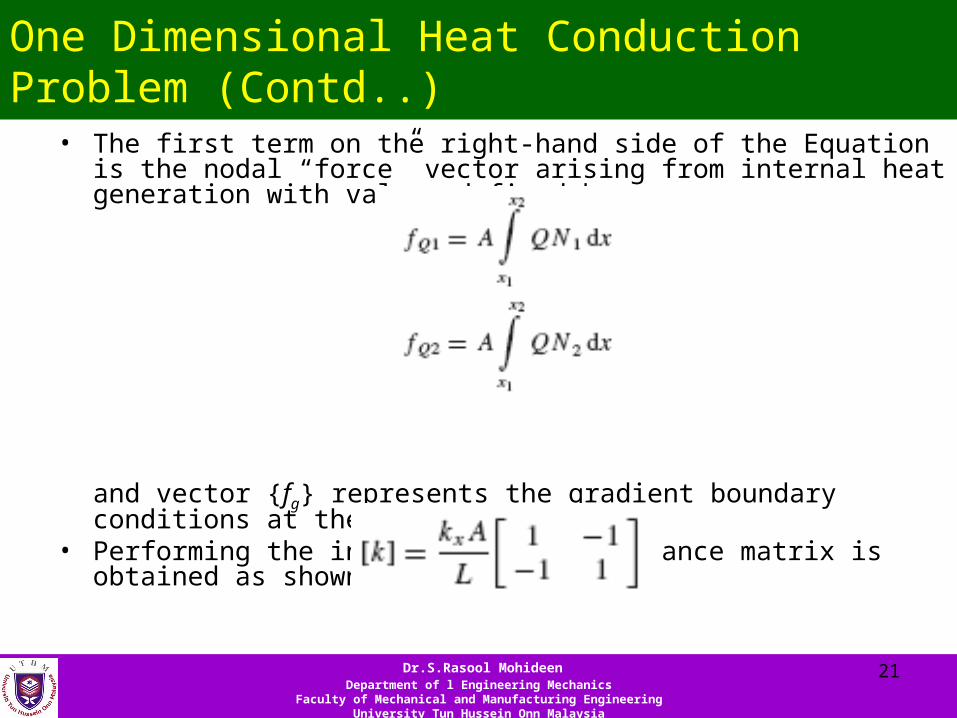
One Dimensional Heat Conduction Problem (Contd..)
• The first term on the right-hand side of the Equation is the nodal “force” vector arising from internal heat generation with values defined by
and vector {fg} represents the gradient boundary conditions at the element nodes.
• Performing the integrations, conductance matrix is obtained as shown below

Dr.S.Rasool MohideenDepartment of l Engineering Mechanics
Faculty of Mechanical and Manufacturing EngineeringUniversity Tun Hussein Onn Malaysia
22
One Dimensional Heat Conduction Problem (Contd..)
• constant internal heat generation (Q) matrix and the element gradient matrix are given as
and

Dr.S.Rasool MohideenDepartment of l Engineering Mechanics
Faculty of Mechanical and Manufacturing EngineeringUniversity Tun Hussein Onn Malaysia
23
Problem 1
• The circular rod shown in Figure has – an outside diameter of 60 mm, – length of 1 m and– is perfectly insulated on its circumference.
• The left half of the cylinder is – aluminum, for which kx = 200 W/m-°C and – the right half is copper having kx = 389 W/m-°C. – The extreme right end of the cylinder is maintained at a temperature
of 80°C, – while the left end is subjected to a heat input rate 4000 W/m2.
• Using four equal-length elements, determine the steady-state temperature distribution in the cylinder.

Dr.S.Rasool MohideenDepartment of l Engineering Mechanics
Faculty of Mechanical and Manufacturing EngineeringUniversity Tun Hussein Onn Malaysia
24
Solution
• The elements and nodes are chosen as shown in the bottom of Figure.
• For aluminum elements 1 and 2, the conductance matrices are
• For copper elements 3 and 4, the conductance matrices are
Dr.S.Rasool MohideenDepartment of l Engineering Mechanics
Faculty of Mechanical and Manufacturing EngineeringUniversity Tun Hussein Onn Malaysia
25
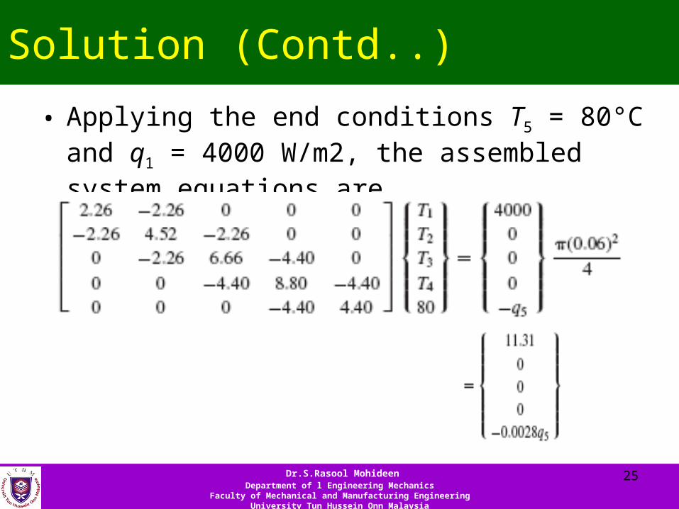
Solution (Contd..)
• Applying the end conditions T5 = 80°C and q1 = 4000 W/m2, the assembled system equations are

Dr.S.Rasool MohideenDepartment of l Engineering Mechanics
Faculty of Mechanical and Manufacturing EngineeringUniversity Tun Hussein Onn Malaysia
26
Solution (Contd..)

Dr.S.Rasool MohideenDepartment of l Engineering Mechanics
Faculty of Mechanical and Manufacturing EngineeringUniversity Tun Hussein Onn Malaysia
27
Solution (Contd..)• Applying the end conditions T5 = 80°C and q1 = 4000 W/m2, the assembled system
equations are
• Accounting for the known temperature at node 5, the first four equations can be written as
• Solving for unknowns, the temperatures areobtained as
• Substituting the unknown (T4) in 5th equation,