ferromagnetic and antiferromagnetic order in bacterial ...dunkel/papers/2016wietal_natphys.pdf ·...

LETTERSPUBLISHED ONLINE: 4 JANUARY 2016 | DOI: 10.1038/NPHYS3607

Ferromagnetic and antiferromagnetic order inbacterial vortex latticesHugoWioland1,2†, Francis G. Woodhouse1,3†, Jörn Dunkel4 and Raymond E. Goldstein1*Despite their inherently non-equilibrium nature1, livingsystems can self-organize in highly ordered collective states2,3that share striking similarities with the thermodynamicequilibrium phases4,5 of conventional condensed-matter andfluid systems. Examples range from the liquid-crystal-likearrangements of bacterial colonies6,7, microbial suspensions8,9and tissues10 to the coherent macro-scale dynamics in schoolsof fish11 and flocks of birds12. Yet, the generic mathematicalprinciples that govern the emergence of structure in suchartificial13 and biological6–9,14 systems are elusive. It is not clearwhen, or even whether, well-established theoretical conceptsdescribing universal thermostatistics of equilibrium systemscan capture and classify ordered states of living matter. Here,we connect these two previously disparate regimes: throughmicrofluidic experiments and mathematical modelling, wedemonstrate that lattices of hydrodynamically coupledbacterial vortices can spontaneously organize into distinctpatterns characterized by ferro- and antiferromagnetic order.The coupling between adjacent vortices can be controlledby tuning the inter-cavity gap widths. The emergence ofopposing order regimes is tightly linked to the existence ofgeometry-induced edge currents15,16, reminiscent of those inquantum systems17–19. Our experimental observations canbe rationalized in terms of a generic lattice field theory,suggesting that bacterial spin networks belong to the sameuniversality class as a wide range of equilibrium systems.

Lattice field theories (LFTs) have been instrumental inuncovering a wide range of fundamental physical phenomena,from quark confinement in atomic nuclei20 and neutron stars21 totopologically protected states of matter22 and transport in novelmagnetic23 and electronic24,25 materials. LFTs can be constructedeither by discretizing the spacetime continuum underlying classicaland quantum field theories20, or by approximating discretephysical quantities, such as the electron spins in a crystal lattice,through continuous variables. In equilibrium thermodynamics,LFT approaches have proved invaluable both computationallyand analytically, for a single LFT often represents a broad classof microscopically distinct physical systems that exhibit thesame universal scaling behaviours in the vicinity of a phasetransition4,26. However, until now there has been little evidenceas to whether the emergence of order in living matter can beunderstood within this universality framework. Our combinedexperimental and theoretical analysis reveals a number of strikinganalogies between the collective cell dynamics in bacterial fluids

and known phases of condensed-matter systems, thereby implyingthat universality concepts may be more broadly applicable thanpreviously thought.

To realize a microbial non-equilibrium LFT, we injected densesuspensions of the rod-like swimming bacterium Bacillus subtilisinto shallow polydimethyl siloxane (PDMS) chambers in whichidentical circular cavities are connected to form one- and two-dimensional (2D) lattice networks (Fig. 1, Supplementary Fig. 6and Methods). Each cavity is 50 µm in diameter and 18 µm deep,a geometry known to induce a stably circulating vortex when adense bacterial suspension is confined within an isolated flatteneddroplet15. For each cavity i, we define the continuous vortex spinvariable Vi(t) at time t as the total angular momentum of the localbacterial flow within this cavity, determined by particle imagingvelocimetry (PIV) analysis (Fig. 1b,f; Supplementary Movies 1and 2 and Methods). To account for the e�ect of oxygenationvariability on suspension motility9, flow velocities are normalizedby the overall root-mean-square (r.m.s.) speed measured in thecorresponding experiment. Bacterial vortices in neighbouringcavities interact through a gap of predetermined width w(Fig. 1f). To explore di�erent interaction strengths, we performedexperiments over a range of gap parameters w (Methods). Forsquare lattices, we varied w from 4 to 25 µm and found that forall but the largest gaps, w w⇤ ⇡20 µm, the suspensions generallyself-organize into coherent vortex lattices, exhibiting domainsof correlated spins whose characteristics depend on couplingstrength (Fig. 1a,e). If the gap size exceeds w⇤, bacteria can movefreely between cavities and individual vortices cease to exist. Here,we focus exclusively on the vortex regime w < w⇤ and quantifypreferred magnetic order through the normalized mean spin–spincorrelation � = h6i⇠jVi(t)Vj(t)/6i⇠j|Vi(t)Vj(t)|i, where 6i⇠jdenotes a sum over pairs {i, j} of adjacent cavities and h · i denotestime average.

Square lattices reveal two distinct states of preferred magneticorder (Fig. 1a,e,i), one with � <0 and the other with � >0,transitioning between them at a critical gap width wcrit ⇡ 8 µm(Fig. 1j). For subcritical values w < wcrit, we observe anantiferromagnetic phase with anti-correlated (� < 0) spinorientations between neighbouring chambers on average (Fig. 1aand Supplementary Movie 1). By contrast, for w >wcrit, spins arepositively correlated (� >0) in a ferromagnetic phase (Fig. 1e andSupplementary Movie 2). Noting that the r.m.s. spin hVi(t)2i1/2decays only slowly with increasing gap width w !w⇤ (Fig. 1k),and that the chambers do not impose any preferred handedness

1Department of Applied Mathematics and Theoretical Physics, University of Cambridge, Wilberforce Road, Cambridge CB3 0WB, UK. 2Institut JacquesMonod, Centre Nationale pour la Recherche Scientifique (CNRS), UMR 7592, Université Paris Diderot, Sorbonne Paris Cité, F-75205 Paris, France. 3Facultyof Engineering, Computing and Mathematics, The University of Western Australia, 35 Stirling Highway, Crawley, Perth, Western Australia 6009, Australia.4Department of Mathematics, Massachusetts Institute of Technology, 77 Massachusetts Avenue, Cambridge, Massachusetts 02139-4307, USA. †Presentaddresses: Institut Jacques Monod, Centre Nationale pour la Recherche Scientifique (CNRS), UMR 7592, Université Paris Diderot, Sorbonne Paris Cité,F-75205 Paris, France (H.W.); Department of Applied Mathematics and Theoretical Physics, University of Cambridge, Wilberforce Road,Cambridge CB3 0WB, UK (F.G.W.). *e-mail: [email protected]

NATURE PHYSICS | ADVANCE ONLINE PUBLICATION | www.nature.com/naturephysics 16

http://dx.doi.org/10.1038/nphys3607

mailto:[email protected]

www.nature.com/naturephysics

LETTERS NATURE PHYSICS DOI: 10.1038/NPHYS3607

P

V

P

V

V

P

V

P

V

V

V

V

V

P

V

P

V

V

P

V

P

V

V

V

V

V

CW

ACW1

0∗∗ ∗

∗∗

−1

Vort

ex sp

in

CW

ACW1

0

−1

Vort

ex sp

in

d

h

c

g

a

e

b

f

0 5 15 20 25wcrit

0.1

0.2

−0.1

−0.2

−0.3

Spin

−spi

n co

rrela

tion

0.0

Gap width (µm) Gap width (µm)

a

e

j

R.m.s. pillar spin0.5

0.6

0.7

R.m

.s. v

orte

x sp

in

0 5 10 15 20 25

0.15

0.20

0.25

ki

Time (s)

Vort

ex sp

in

0

1

−1

01

−10 2 4 6 8 10

Gapwidth

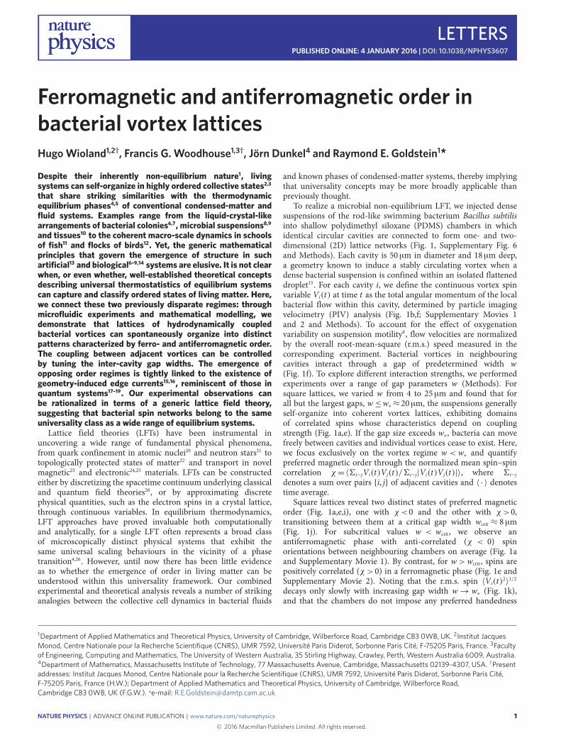
Figure 1 | Edge currents determine antiferromagnetic and ferromagnetic order in a square lattice of bacterial vortices. a, Three domains ofantiferromagnetic order highlighted by dashed white lines (gap width w=6 µm). Scale bar, 50 µm. Overlaid false colour shows spin magnitude (seeSupplementary Movie 1 for raw data). b, Bacterial flow PIV field within an antiferromagnetic domain (Supplementary Movie 1). For clarity, not all velocityvectors are shown. Largest arrows correspond to speed 40 µm s�1. Scale bar, 20 µm. c, Schematic of bacterial flow circulation in the vicinity of a gap. Forsmall gaps w<wcrit, bacteria forming the edge currents (blue arrows) swim across the gap, remaining in their original cavity. Bulk flow (red) is directedopposite to the edge current15,16 (Supplementary Movie 3). d, Graph of the Union Jack double-lattice model in an antiferromagnetic state with zero netpillar circulation. Solid and dashed lines depict vortex–vortex and vortex–pillar interactions of respective strengths Jv and Jp. Vortices and pillars arecolour-coded according to their spin. e, For supercritical gap widths w>wcrit, extended domains of ferromagnetic order predominate (SupplementaryMovie 2; w= 11 µm). Scale bar, 50 µm. f, PIV field within a ferromagnetic domain (Supplementary Movie 2). Largest arrows: 36 µm s�1. Scale bar, 20 µm.g, For w>wcrit, bacteria forming the edge current (blue arrows) swim along the PDMS boundary through the gap, driving bulk flows (red) in the oppositedirections, thereby aligning neighbouring vortex spins. h, Ferromagnetic state of the Union Jack lattice induced by edge current loops around the pillars.i, Trajectories of neighbouring spins (⇤-symbols in a,e) fluctuate over time, signalling exploration of a fluctuating steady state under a non-zero e�ectivetemperature (top, antiferromagnetic; bottom, ferromagnetic). j, The zero of the spin–spin correlation � at wcrit ⇡8 µm marks the phase transition. Thebest-fit Union Jack model (solid line) is consistent with the experimental data. k, R.m.s. vortex spin hV2

i i1/2 decreases with the gap size w, showingweakening of the circulation. R.m.s. pillar spin hP2

j i1/2 increases with w, reflecting enhanced bacterial circulation around pillars. Each point in j,k representsan average over �5 movies in 3 µm bins at 1.5 µm intervals; vertical bars indicate standard errors (Methods).

on the vortex spins (Supplementary Fig. 1 and SupplementarySection 1), we conclude that the observed phase behaviour iscaused by spin–spin interactions. However, although both phasespossess a well-defined average vortex–vortex correlation, theindividual spins fluctuate randomly over time as ordered domainssplit, merge and flip (Fig. 1i and Supplementary Figs 1 and 3)while the system explores configuration space inside a statisticalsteady state (Supplementary Sections 1 and 3). Thus, althoughthe bacterial vortex spins {Vi(t)} define a real-valued lattice field,the phenomenology of these continuous bacterial spin lattices isqualitatively similar to that of the classical 2D Ising model4 withdiscrete binary spin variables si 2 {±1}, whose configurationalprobability at finite temperature T = (kB�)�1 is described by athermal Boltzmann distribution / exp(��J6i⇠jsisj), where J > 0corresponds to ferromagnetic and J <0 to antiferromagnetic order.The detailed theoretical analysis below shows that the observedphases in the bacterial spin system can be understood quantitativelyin terms of a generic quartic LFT comprising two dual interacting

lattices. The introduction of a double lattice is necessitated by themicroscopic structure of the underlying bacterial flows. By analogywith a lattice of interlocking cogs, one might have intuitivelyexpected that the antiferromagnetic phase would generally befavoured, because only in this configuration does the bacterialflow along the cavity boundaries conform across the inter-cavitygap, avoiding the potentially destabilizing head-to-head collisionsthat would occur with opposing flows (Fig. 1b,c). However, theextent of the observed ferromagnetic phase highlights a competingbiofluid-mechanical e�ect.

Just as the quantum Hall e�ect17 and the transport propertiesof graphene18,19 arise from electric edge currents, the opposingorder regimes observed here are explained by the existence ofanalogous bacterial edge currents. At the boundary of an isolatedflattened droplet of a bacterial suspension, a single layer of cells—an edge current—can be observed swimming against the bulkcirculation15,16. This narrow cell layer is key to the suspensiondynamics: the hydrodynamics of the edge current circulating

2 NATURE PHYSICS | ADVANCE ONLINE PUBLICATION | www.nature.com/naturephysics6



NATURE PHYSICS DOI: 10.1038/NPHYS3607 LETTERSin one direction advects nearby cells in the opposite direction,which in turn dictate the bulk circulation by flow continuitythrough steric and hydrodynamic interactions16,27. Identical edgecurrents are present in our lattices (Supplementary Movie 3) andexplain both order regimes as follows. In the antiferromagneticregime, when w < wcrit, the bacterial edge current driving aparticular vortex will pass over the gap without leaving the cavity(Fig. 1c). Interaction with a neighbouring edge current throughthe gap favours parallel flow, inducing counter-circulation ofneighbouring vortices and therefore driving antiferromagneticorder (Fig. 1d). However, when w > wcrit, the edge currentscan no longer pass over the gaps and instead wind around thestar-shaped pillars dividing the cavities (Fig. 1g). A clockwise(resp. anticlockwise) bacterial edge current about a pillar inducesanticlockwise (resp. clockwise) fluid circulation about the pillarin a thin region near its boundary. Flow continuity then inducesclockwise (resp. anticlockwise) flow in all cavities adjacent to thepillar, resulting in ferromagnetic order (Fig. 1h). Thus by viewingthe system as an anti-cooperative Union Jack lattice28,29 of both bulkvortex spins Vi and near-pillar circulations Pj, we accommodateboth order regimes: antiferromagnetism as indefinite circulationsPj =0 and alternating spins Vi =±V (Fig. 1d), and ferromagnetismas definite circulations Pj =�P < 0 and uniform spins Vi =V > 0(Fig. 1h). To verify these considerations, we determined the netnear-pillar circulation Pj(t) using PIV (Methods) and found thatthe r.m.s. circulation hPj(t)2i1/2 shows the expected monotonicincrease as the inter-cavity gap widens (Fig. 1k).

Competition between the vortex–vortex and vortex–pillarinteractions determines the resultant order regime. Their relativestrengths can be inferred by mapping each experiment onto acontinuous-spin Union Jack lattice (Fig. 1d,h). In this model, theinteraction energy of the time-dependent vortex spins V={Vi} andpillar circulations P={Pj} is defined by the LFT Hamiltonian

H(V,P) = �JvX

Vi⇠Vj

ViVj � JpX

Vi⇠Pj

ViPj

+X

Vi

✓12avV 2

i + 14bvV 4

i

◆+X

Pj

12apP2

j (1)

The first two sums are vortex–vortex and vortex–pillar interactionswith strengths Jv, Jp <0, where ⇠ denotes adjacent lattice pairs. Thelast two sums are individual vortex and pillar circulation potentials.Vortices must be subject to a quartic potential function with bv >0to allow for a potentially double-welled potential if av <0, encodingthe observed symmetry breaking into spontaneous circulationin the absence of other interactions15,27. In contrast, our dataanalysis implies that pillar circulations are su�ciently describedby a quadratic potential of strength ap > 0 (Supplementary Fig. 4and Supplementary Section 4). To account for the experimentallyobserved spin fluctuations (Fig. 1i and Supplementary Fig. 1), wemodel the dynamics of the lattice fieldsV andP through the coupledstochastic di�erential equations (SDEs)

dV=�(@H/@V)dt+p2TvdWv (2)

dP=�(@H/@P)dt+p2TpdWp (3)

where Wv and Wp are vectors of uncorrelated Wiener processesrepresenting intrinsic and thermal fluctuations. The overdampeddynamics in equations (2) and (3) neglects dissipative Onsager-type cross-couplings, as the dominant contribution to frictionstems from the nearby no-slip PDMS boundaries (SupplementarySection 7). The parameters Tv and Tp set the strength of

random perturbations from energy-minimizing behaviour. In theequilibrium limit when Tv =Tp =T , the stationary statistics of thesolutions of equations (2) and (3) obey the Boltzmann distribution/e�H/T . We inferred all seven parameters of the full SDE modelfor each experiment by linear regression on a discretization ofthe SDEs (Supplementary Fig. 2 and Supplementary Section 2).The di�ering sublattice temperatures Tv 6= Tp found show thatthe system is not in thermodynamic equilibrium owing to itsactive microscopic constituents (Supplementary Fig. 2). Instead,the system is in a pseudo-equilibrium statistical steady state(Supplementary Section 1), which we will soon show can bereduced to an equilibrium-like description. As a cross-validation,we fitted appropriate functions of gapwidthw to these estimates andsimulated the resulting SDEmodel over a range ofw on a 6⇥6 latticeconcordant with the observations (Supplementary Section 3). Theagreement between experimental data and the numerically obtainedvortex–vortex correlation �(w) supports the validity of the double-lattice model and its underlying approximations (Fig. 1j).

To reconnect with the classical 2D Ising model and understandbetter the experimentally observed phase transition, we projectthe Hamiltonian (1) onto an e�ective square lattice model bymaking a mean-field assumption for the pillar circulations. Inthe experiments, Pi is linearly correlated with the average spinof its vortex neighbours [Pi]V = (1/4)6j :Vj⇠PiVj, with a constantof proportionality �↵ < 0 only weakly dependent on gap width(Supplementary Fig. 4 and Supplementary Section 4). Replacinge�ectively Pi ! �↵[Pi]V as a mean-field variable in the modeleliminates all pillar circulations, yielding a standard quartic LFTfor V (see Supplementary Section 4 for a detailed derivation).The mean-field dynamics are then governed by the reducedSDE dV = �(@H/@V) dt + p

2TdW with e�ective temperatureT ⇡Tv +4TpJ 2p /a2p and energy

H(V)=�JX

Vi⇠Vj

ViVj +X

Vi

✓12aV 2

i + 14bV 4

i

◆

which has steady-state probability density p(V) / e��H with� =1/T , and where a = av � 4J 2p /ap and b = bv . Note thatin the limit a ! �1 and b ! +1 with a/b fixed, theclassical two-state Ising model is recovered by identifyingsi =Vi/

p|a|/b2{±1}. The reduced coupling constant J relates tothose of the double-lattice model (Jv, Jp) in the thermodynamiclimit as J ⇡ Jv � (1/2)↵Jp (Supplementary Section 4), makingmanifest how competition between Jv and Jp can result inboth antiferromagnetic (|Jv| > (1/2)↵|Jp|) or ferromagnetic(|Jv| < (1/2)↵|Jp|) behaviour. We estimated �J , �a and �bfor each experiment by directly fitting the e�ective one-spinpotential V e�(V | [V ]V ) = �4�JV [V ]V + (1/2)�aV 2 + (1/4)�bV 4

via the log-likelihood logp(V | [V ]V )=�V e� +const (Fig. 2,Supplementary Fig. 5 and Supplementary Section 5). Theseestimates match those obtained independently using SDEregression methods (Fig. 2a–c and Supplementary Section 5), andshow the transition from antiferromagnetic interaction (�J < 0)to ferromagnetic interaction (�J > 0) at wcrit (Fig. 2a). As the gapwidth increases, the energy barrier to spin change falls (Fig. 2b)and the magnitude of the lowest energy spin decreases (Fig. 2c)as a result of weakening confinement within each cavity, visible asa flattening of the one-spin e�ective potential V e� (Fig. 2d–f andSupplementary Fig. 5).

Experiments on lattices of di�erent symmetry groups lendfurther insight into the competition between edge currents and bulkflow. Unlike their square counterparts, triangular lattices cannotsupport antiferromagnetic states without frustration. Therefore,ferromagnetic order should be enhanced in a triangular bacterialspin lattice. This is indeed observed in our experiments: atmoderate gap size w . 18 µm, we found exclusively a highly





a cb

0 5 10 15 20 25Gap width (µm)

0 5 10 15 20 25Gap width (µm)

0 5 10 15 20 25Gap width (µm)

0.2

0.4

0.6

0.0

−0.2

−0.4

E�ec

tive

inte

ract

ion

0.5

0.0

1.0

Ener

gy b

arrie

r

0.0

0.2

0.4

0.6

0.8

Spin

of m

inim

um e

nerg

y

0

4

−4

8

−10

1

−10

1

0.0

Meanadjacent spin

Meanadjacent spin

0.40.8

Vortex spinVortex spin

E�ec

tive

pote

ntia

l

d e f

0

4

−4

8

0.00.4

0.8E�

ectiv

e po

tent

ial

−10

1Meanadjacent spin Vortex spin

0

4

−4

8

0.00.4

0.8

E�ec

tive

pote

ntia

l

Figure 2 | Best-fit mean-field LFT model captures the phase transition in the square lattice. a, A sign change of the e�ective interaction �J signals thetransition from antiferro- to ferromagnetic states. b, The e�ective energy barrier, �a2/(4b) when a<0 and zero when a>0 (Supplementary Section 5),decreases with the gap size w, reflecting increased susceptibility to fluctuations. c, The spin Vmin minimizing the single-spin potential (SupplementarySection 5) decreases with w in agreement with the decrease in the r.m.s. vortex spin (Fig. 1k). Each point in a–c represents an average over �5 movies in3 µm bins at 1.5 µm intervals; blue circles are from distribution fitting, red diamonds are from SDE regression, and vertical bars indicate standard errors(Methods). d–f, Examples of the e�ective single-spin potential Ve� conditional on the mean spin of adjacent vortices [V]V . Data (points) and estimatedpotential (surface) for three movies with gap widths 6, 10 and 17 µm.

ba

c

0 10 20 30Gap width, w (µm)

Spin

−spi

n co

rrela

tion

0.0

0.5

1.0

−0.5a b

d

CW ACW10−1

Vortex spin

c

Figure 3 | Frustration in triangular lattices determines the preferred order.a,b, Triangular lattices favour ferromagnetic states of either handedness(Supplementary Movie 4). Vortices are colour-coded by spin. c, At thelargest gap size, bacterial circulation becomes unstable. Scale bar, 50 µm.d, The spin–spin correlation � shows strongly enhanced ferromagneticorder compared with the square lattice (Fig. 1j). Each point represents anaverage over �5 movies in 3 µm bins at 1.5 µm intervals; vertical barsindicate standard errors (Methods).

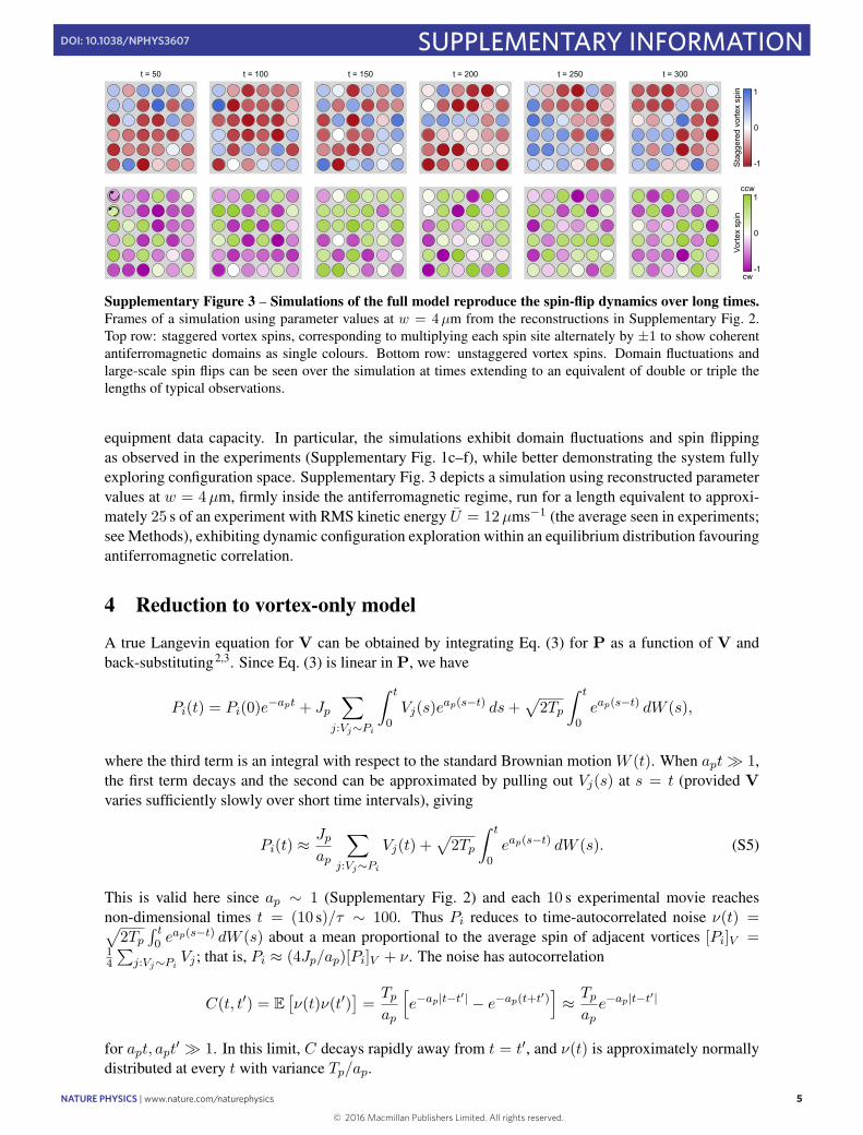
robust ferromagnetic phase of either handedness (Fig. 3a,b,d andSupplementary Movie 4), reminiscent of quantum vortex latticesin Bose–Einstein condensates30. At comparable gap size, the spincorrelation is approximately four to eight times larger than in thesquare lattice. Increasing the gap size beyond 20 µm eventuallydestroys the spontaneous circulation within the cavities and adisordered state prevails (Fig. 3c,d), with a sharper transitionthan for the square lattices (Fig. 1j). Conversely, a 1D line latticeexclusively exhibits antiferromagnetic order as the suspension isunable to maintain the very long uniform edge currents thatwould be necessary to sustain a ferromagnetic state (SupplementaryFig. 6 and Supplementary Section 6). These results manifest theimportance of lattice geometry and dimensionality for vortexordering in bacterial spin lattices, in close analogy with theirelectromagnetic counterparts.

Understanding the ordering principles of microbial matter is akey challenge in active materials design13, quantitative biology andbiomedical research. Improved prevention strategies for pathogenicbiofilm formation, for example, will require detailed knowledge ofhow bacterial flows interact with complex porous surface structuresto create the stagnation points at which biofilms can nucleate. Ourstudy shows that collective excitations in geometrically confinedbacterial suspensions can spontaneously organize in phases ofmagnetic order that can be robustly controlled by edge currents.These results demonstrate fundamental similarities with a broadclass of widely studied quantum systems17,19,30, suggesting thattheoretical concepts originally developed to describe magnetism indisordered media could potentially capture microbial behaviours incomplex environments. Future studiesmay try to explore further therange and limits of this promising analogy.

MethodsMethods and any associated references are available in the onlineversion of the paper.

4 NATURE PHYSICS | ADVANCE ONLINE PUBLICATION | www.nature.com/naturephysics6





NATURE PHYSICS DOI: 10.1038/NPHYS3607 LETTERSReceived 11 June 2015; accepted 13 November 2015;published online 4 January 2016

References1. Schrödinger, E.What is Life? (Cambridge Univ. Press, 1944).2. Vicsek, T. & Zafeiris, A. Collective motion. Phys. Rep. 517, 71–140 (2012).3. Marchetti, M. C. et al . Hydrodynamics of soft active matter. Rev. Mod. Phys. 85,

1143–1189 (2013).4. Kardar, M. Statistical Physics of Fields (Cambridge Univ. Press, 2007).5. Mermin, N. D. The topological theory of defects in ordered media. Rev. Mod.

Phys. 51, 591–648 (1979).6. Ben Jacob, E., Becker, I., Shapira, Y. & Levine, H. Bacterial linguistic

communication and social intelligence. Trends Microbiol. 12, 366–372 (2004).7. Volfson, D., Cookson, S., Hasty, J. & Tsimring, L. S. Biomechanical ordering of

dense cell populations. Proc. Natl Acad. Sci. USA 150, 15346–15351 (2008).8. Riedel, I. H., Kruse, K. & Howard, J. A self-organized vortex array of

hydrodynamically entrained sperm cells. Science 309, 300–303 (2005).9. Dunkel, J. et al . Fluid dynamics of bacterial turbulence. Phys. Rev. Lett. 110,

228102 (2013).10. Wu, J., Roman, A.-C., Carvajal-Gonzalez, J. M. & Mlodzik, M. Wg and Wnt4

provide long-range directional input to planar cell polarity orientation indrosophila. Nature Cell Biol. 15, 1045–1055 (2013).

11. Katz, Y., Ioannou, C. C., Tunstro, K., Huepe, C. & Couzin, I. D. Inferring thestructure and dynamics of interactions in schooling fish. Proc. Natl Acad. Sci.USA 108, 18720–18725 (2011).

12. Cavagna, A. et al . Scale-free correlations in starling flocks. Proc. Natl Acad. Sci.USA 107, 11865–11870 (2010).

13. Sanchez, T., Chen, D. T. N., DeCamp, S. J., Heymann, M. & Dogic, Z.Spontaneous motion in hierarchically assembled active matter. Nature 491,431–434 (2012).

14. Sokolov, A. & Aranson, I. S. Physical properties of collective motion insuspensions of bacteria. Phys. Rev. Lett. 109, 248109 (2012).

15. Wioland, H., Woodhouse, F. G., Dunkel, J., Kessler, J. O. & Goldstein, R. E.Confinement stabilizes a bacterial suspension into a spiral vortex. Phys. Rev.Lett. 110, 268102 (2013).

16. Lushi, E., Wioland, H. & Goldstein, R. E. Fluid flows created by swimmingbacteria drive self-organization in confined suspensions. Proc. Natl Acad. Sci.USA 111, 9733–9738 (2014).

17. Büttiker, M. Absence of backscattering in the quantum Hall e�ect inmultiprobe conductors. Phys. Rev. B 38, 9375–9389 (1988).

18. Kane, C. L. & Mele, E. J. Quantum spin Hall e�ect in graphene. Phys. Rev. Lett.95, 226801 (2005).

19. Castro Neto, A. H., Guinea, F., Peres, N. M. R., Novoselov, K. S. & Geim, A. K.The electronic properties of graphene. Rev. Mod. Phys. 81, 109–162 (2009).

20. Wilson, K. G. Confinement of quarks. Phys. Rev. D 10, 2445–2459 (1974).21. Glendenning, N. K. Compact Stars: Nuclear Physics, Particle Physics, and

General Relativity (Springer, 2000).22. Battye, R. A. & Sutcli�e, P. M. Skyrmions with massive pions. Phys. Rev. C 73,

055205 (2006).23. Nagaosa, N. & Tokura, Y. Topological properties and dynamics of magnetic

skyrmions. Nature Nanotech. 8, 899–911 (2013).24. Novoselov, K. S. et al . Two-dimensional gas of massless Dirac fermions in

graphene. Nature 438, 197–200 (2005).25. Drut, J. E. & Lähde, T. A. Lattice field theory simulations of graphene. Phys.

Rev. B 79, 165425 (2009).26. Fernández, R., Fröhlich, J. & Sokal, A. D. RandomWalks, Critical Phenomena,

and Triviality in Quantum Field Theory (Springer, 1992).27. Woodhouse, F. G. & Goldstein, R. E. Spontaneous circulation of confined active

suspensions. Phys. Rev. Lett. 109, 168105 (2012).28. Vaks, V. G., Larkin, A. I. & Ovchinnikov, Y. N. Ising model with interaction

between non-nearest neighbors. Sov. Phys. JETP 22, 820–826 (1966).29. Stephenson, J. Ising model with antiferromagnetic next-nearest-neighbor

coupling: spin correlations and disorder points. Phys. Rev. B 1,4405–4409 (1970).

30. Abo-Shaeer, J. R., Raman, C., Vogels, J. M. & Ketterle, W. Observation of vortexlattices in Bose–Einstein condensates. Science 292, 476–479 (2001).

AcknowledgementsWe thank V. Kantsler and E. Lushi for assistance and discussions. This work wassupported by European Research Council Advanced Investigator Grant 247333 (H.W.and R.E.G.), EPSRC (H.W. and R.E.G.), an MIT Solomon Buchsbaum Fund Award (J.D.)and an Alfred P. Sloan Research Fellowship (J.D.).

Author contributionsAll authors designed the research and collaborated on theory. H.W. performedexperiments and PIV analysis. H.W. and F.G.W. analysed PIV data and performedparameter inference. F.G.W. and J.D. wrote simulation code. All authors wrotethe paper.

Additional informationSupplementary information is available in the online version of the paper. Reprints andpermissions information is available online at www.nature.com/reprints.Correspondence and requests for materials should be addressed to R.E.G.

Competing financial interestsThe authors declare no competing financial interests.




http://www.nature.com/reprints



MethodsExperiments.Wild-type Bacillus subtilis cells (strain 168) were grown in TerrificBroth (Sigma). A monoclonal colony was transferred from an agar plate to 25ml ofmedium and left to grow overnight at 35 �C on a shaker. The culture was diluted200-fold into fresh medium and harvested after approximately 5 h, when more than90% of the bacteria were swimming, as visually verified on a microscope. 10ml ofthe suspension was then concentrated by centrifugation at 1,500g for 10min,resulting in a pellet with volume fraction approximately 20% which was usedwithout further dilution.

The microchambers were made of polydimethyl siloxane (PDMS) bound to aglass coverslip by oxygen plasma etching. These comprised a square, triangular orlinear lattice of ⇠18-µm-deep circular cavities with 60 µm between centres, each ofdiameter ⇠50 µm, connected by 4–25-µm-wide gaps for linear and square lattices(Fig. 1a,e and Supplementary Fig. 6) and 10–25-µm-wide gaps for triangular lattices(Fig. 3a–c). The smallest possible gap size was limited by the fidelity of the etching.

Approximately 5 µl of the concentrated suspension was manually injected intothe chamber using a syringe. Both inlets were then sealed to prevent external flow.We imaged the suspension on an inverted microscope (Zeiss, Axio Observer Z1)under bright-field illumination, through a 40⇥ oil-immersion objective. Movies10 s in length were recorded at 60 f.p.s. on a high-speed camera (Photron FastcamSA3) at 4 and 8min after injection. Although the PDMS lattices were typically ⇠15cavities across, to avoid boundary e�ects and to attain the pixel density necessaryfor PIV we imaged a central subregion spanning 6⇥6 cavities for square lattices,7⇥6 cavities for triangular lattices, and 7 cavities for linear lattices (multiple ofwhich were captured on a single slide).

Fluorescence in Supplementary Movie 3 was achieved by labelling themembranes of a cell subpopulation with fluorophore FM4-64 following theprotocol of Lushi et al.16 The suspension was injected into an identical triangularlattice as in the primary experiments and imaged at 5.6 f.p.s. on a spinning-discconfocal microscope through a 63⇥ oil-immersion objective.

Analysis. For each frame of each movie, the bacterial suspension flow fieldu(x ,y , t) was measured by standard particle image velocimetry (PIV) without timeaveraging, using a customized version of mPIV (http://www.oceanwave.jp/softwares/mpiv). PIV subwindows were 16⇥16 pixels with 50% overlap, yielding⇠150 vectors per cavity per frame. Cavity regions were identified in each movie bymanually placing the centre and radius of the bottom left cavity, measuring vectorsto its immediate neighbours, and repeatedly translating to generate the full grid.Pillar edges were then calculated from the cavity grid and the gap width (measuredas the minimum distance between adjacent pillars).

The spin Vi(t) of each cavity i at time t is defined as the normalized planarangular momentum

Vi(t)=z ·

hP(x ,y)i ri(x ,y)⇥u(x ,y , t)

i

UP

(x ,y)i |ri(x ,y)|

where ri(x ,y) is the vector from the cavity centre to (x ,y), and sums run over allPIV grid points (x ,y)i inside cavity i. For each movie, we normalize velocities bythe root-mean-square (r.m.s.) suspension velocity U = hu(x ,y , t)2i1/2, where theaverage is over all grid points (x ,y) and all times t , to account for the e�ects ofvariable oxygenation on motility9; we found an ensemble averageE[U ]=12.1 µms�1 with s.d. 3.6 µms�1 over all experiments. This definition hasVi(t)>0 for anticlockwise spin and Vi(t)<0 for clockwise spin. A vortex ofradially independent speed—that is, u(x ,y , t)=u✓ , where ✓ is the azimuthal unitvector—has Vi(t)=±1; conversely, randomly oriented flow has Vi(t)=0. Theaverage spin–spin correlation � of a movie is then defined as

� =* P

i⇠j Vi(t)Vj(t)Pi⇠j |Vi(t)Vj(t)|

+

where 6i⇠j denotes a sum over pairs {i, j} of adjacent cavities and h·i denotes anaverage over all frames. If all vortices share the same sign, then � =1(ferromagnetism); if each vortex is of opposite sign to its neighbours, then � =�1(antiferromagnetism); if the vortices are uniformly random, then � =0. Similarly,the circulation Pj(t) about pillar j at time t is defined as the normalized averagetangential velocity

Pj(t)=P

(x ,y)j u(x ,y , t) · tj(x ,y)UP

(x ,y)j 1

where tj(x ,y) is the unit vector tangential to the pillar, and sums run over PIV gridpoints (x ,y)j closer than 5 µm to the pillar j.

Results presented are typically averaged in bins of fixed gap width. All plotswith error bars use 3 µm bins, calculated every 1.5 µm (50% overlap), and bins withfewer than five movies were excluded. Error bars denote standard error. Bin countsfor square lattices (Figs 1j,k and 2a–c and Supplementary Figs 4 and 7) are 8, 8, 13,14, 21, 27, 27, 22, 18, 22, 20, 11, 7, 13, 7; bin counts for triangular lattices (Fig. 3d)are 5, 14, 16, 13, 16, 15, 5, 5, 10, 7; and bin counts for linear lattices (SupplementaryFig. 6) are 5, 7, 8, 8, 9, 9, 6, 5, 6, 7, 6, 8, 9, 5, 6, 5, 6.

NATURE PHYSICS | www.nature.com/naturephysics6


http://www.oceanwave.jp/softwares/mpiv

http://www.oceanwave.jp/softwares/mpiv


Ferromagnetic and antiferromagnetic order in bacterial vortex latticesSupplementary information

Hugo Wioland1,2† , Francis G. Woodhouse1†,3, Jorn Dunkel4, and Raymond E. Goldstein1

1Department of Applied Mathematics and Theoretical Physics, University of Cambridge, WilberforceRoad, Cambridge CB3 0WB, U.K.2Institut Jacques Monod, Centre Nationale pour la Recherche Scientifique (CNRS), UMR 7592, Uni-versite Paris Diderot, Sorbonne Paris Cite, F-75205 Paris, France3Faculty of Engineering, Computing and Mathematics, The University of Western Australia, 35 StirlingHighway, Crawley, Perth WA 6009, Australia4Department of Mathematics, Massachusetts Institute of Technology, 77 Massachusetts Avenue, Cam-bridge MA 02139-4307, U.S.A.†Present address.

1 Experimental consistency with theoretical model

In populating our chosen theoretical models, we make important assumptions of the experimental dataconcerning spin bias, statistical steadiness, and phase-space exploration. In the following, we discussthese assumptions and provide evidence for their validity.

1.1 Absence of spin handedness bias

In the Hamiltonian (1), we assume a symmetric local quartic potential. For this to be valid, the vorticesmust be free of any handedness bias that might be induced by interactions between the chiral bacteriaand the upper and lower surfaces of the chamber. Plotting a histogram of the time-averaged spins acrossall experiments shows no discernible bias towards either vorticity handedness (Supplementary Fig. 1a),so this assumption is justified.

1.2 Statistical steady state

When estimating parameters using movies taken after 4 and 8 minutes with equal weight, we are as-suming that the suspension has reached a sufficiently statistically-steady state no later than 4 minutesafter injection. We checked this assumption by comparing the spin–spin correlation in movies takenat 4 and 8 minutes with identically acquired movies taken 1 minute after injection. We found that themean correlation changed much less between 4 and 8 minutes than between 1 and 4 minutes for experi-ments both below and above the critical transition gap size (Supplementary Fig. 1b), indicating sufficientequilibration to perform parameter estimation at both 4 and 8 minutes independently.

1.3 Phase-space exploration

A system following an equilibrium-like description such as the model in Eqs. (2) and (3) will not befrozen into one configuration for all time. Rather, given sufficient time, it should explore all states ofits configuration space according to a steady-state probability distribution. Our experiments show thisexploration behaviour, with spins fluctuating and changing sign over time (Supplementary Fig. 1e,f).This is particularly noticeable when comparing between the same experiment at the two observationtimes of 4 and 8 minutes, during which time some (Supplementary Fig. 1c) or most (SupplementaryFig. 1d) spins may have changed orientation. However, the system is always exploring a distributionconsistent with a particular preferred antiferromagnetic or ferromagnetic correlation, dependent on thegap size.

1

Ferromagnetic and antiferromagnetic order in bacterial vortex lattices












1












1












1












1

SUPPLEMENTARY INFORMATIONDOI: 10.1038/NPHYS3607

NATURE PHYSICS | www.nature.com/naturephysics 1

6

0

0.05

0.10

-0.05

-0.10

-0.15

-0.20

w < wcrit w > wcrit

Mea

n sp

in-s

pin

corr

elat

ion

1 min4 min8 min

Vorte

x sp

in

0

1

-1

4 min

Time (s)

0

1

-10 2 4 6 8 10

Vorte

x sp

in

4 min

8 min

Time (s)0 2 4 6 8 10

8 min

cw

ccw1

0

-1

Vorte

x sp

in

4 min 8 min

0 0.5 1-0.5-1Mean ortex spin

0

100

200

00

reen

c400

500

b

e

f

d

a c

cw

ccw1

0

-1

Vorte

x sp

in

4 min 8 min

Supplementary Figure 1 – Experiments are unbiased and explore a statistical steady state. a, Histogram oftime-averaged vortex spin of each cavity ⟨Vi(t)⟩ across all square lattice experiments, exhibiting symmetry aboutzero spin. b, Spin–spin correlation χ averaged over all movies taken 1, 4 or 8min after injection, categorised bygap size w < wcrit or w > wcrit. The suspension is not equilibrated 1min after injection, but results are similarbetween 4 and 8min indicating equilibration. c,d, Frames from movies taken from two experiments at 4 and8min, with w = 7µm (c) and w = 11µm (d), showing phase-space exploration between the observation times.e,f, Spin–time traces of four adjacent vortices from the experiments shown in c,d (line colours correspond to starcolours in c,d).

2 Parameter inference under the full model

For a given sequence of discrete experimental observations {V(t),P(t)}t=n∆t derived from one moviewith constant time step ∆t = 1/60 s and rescaled by U (Methods), we wish to estimate the most likelyparameter values assuming the SDE model in Eqs. (2) and (3) holds. We do this by first discretizingEqs. (2) and (3) and then applying linear regression. First, the rescaling by U used to eliminate variableoxygenation effects (Methods) implies that we must also rescale the time step to δt = ∆t/τ , whereτ = ℓ/U is a time scaling with length scale ℓ = 1µm selected as the characteristic width of a bacterium.All parameters are subsequently dimensionless under these scalings; those for an unscaled experiment(denoted by tildes) with desired or observed RMS velocity U can then be recovered as Jv = Jv/τ ,Jp = Jp/τ , av = av/τ , bv = bv/(U

2τ), ap = ap/τ , Tv = U

2Tv/τ and Tp = U

2Tp/τ . Now, using this

time step, Eqs. (2) and (3) discretize in the Euler–Maruyama scheme1 as

V(t+ δt) = V(t)− (∂H/∂V)tδt+√

2TvδtNv, (S1)

P(t+ δt) = P(t)− (∂H/∂P)tδt+√

2TpδtNp, (S2)

where Nv and Np are vectors of independent N (0, 1) random variables. Component-wise, Eqs. (S1)and (S2) read

Vi(t+ δt) = (1− avδt)Vi(t)− bvδtVi(t)3

+ Jvδt∑

j :Vj∼Vi

Vj(t) + Jpδt∑

j :Pj∼Vi

Pj(t) +√2TvδtNv,i, (S3)

Pi(t+ δt) = (1− apδt)Pi(t) + Jpδt∑

j :Vj∼Pi

Vj(t) +√

2TpδtNp,i. (S4)

By Eq. (S4), using data from all observation times and vortices to perform a linear regression of Pi(t+δt)on the two variables

⎧⎨

⎩Pi(t),∑

j :Vj∼Pi

Vj(t)

⎫⎬

⎭

yields estimates {1− apδt, Jpδt} of the variables’ respective coefficients and thence estimates ap and Jpof ap and Jp. Next, after substituting the estimate Jp = Jp into Eq. (S3) to reduce the dimensionality, alinear regression of Vi(t+ δt)− Jpδt

∑j :Pj∼Vi

Pj(t) on the three variables⎧⎨

⎩Vi(t), Vi(t)3,

∑

j :Vj∼Vi

Vj(t)

⎫⎬

⎭

yields estimates {1− avδt,−bvδt, Jvδt} of their respective coefficients and thence estimates av, bv andJv of av, bv and Jv. Finally, the variances 2Tvδt and 2Tpδt of the residuals to the regressions in Eqs. (S3)and (S4) respectively yield estimates Tv and Tp of Tv and Tp.

Boundary terms are treated by assuming a truly finite system with free boundary conditions, effec-tively fixing all pillar and vortex spins at zero outside of the observed domain. Since we do not image afull 6× 6 offset lattice of pillars, but instead the internal 5× 5 lattice, periodic boundary conditions arenot possible; indeed, for a small system, free boundaries are often preferable over periodic boundariesin general.

3 Simulations

To reconstruct the vortex–vortex correlation function χ(w) as a continuous function of gap width w, wereconstructed the parameters as functions of w from the experimental data and numerically integratedthe model in Eqs. (2) and (3) over a range of w. The simulations can then be used to explore the systemon longer time scales than possible experimentally. We discuss this process further in the followingsection.

3.1 Parameter reconstruction

Running the parameter estimation procedure for every suitable experimental movie (those not contain-ing any ‘locked’ immobile cavities, occasionally seen at small w) results in a set of parameter estimatesEi at gaps wi. Estimates for movies from the same experiment were averaged, and then placed into non-overlapping w-bins of size 2.5µm and averaged in both w and parameter value within each bin (Supple-mentary Fig. 2, points). Using non-linear least-squares regression estimation, the parameters were then

3

2 NATURE PHYSICS | www.nature.com/naturephysics

SUPPLEMENTARY INFORMATION DOI: 10.1038/NPHYS3607

6

time step, Eqs. (2) and (3) discretize in the Euler–Maruyama scheme1 as

V(t+ δt) = V(t)− (∂H/∂V)tδt+√2TvδtNv, (S1)

P(t+ δt) = P(t)− (∂H/∂P)tδt+√2TpδtNp, (S2)

where Nv and Np are vectors of independent N (0, 1) random variables. Component-wise, Eqs. (S1)and (S2) read

Vi(t+ δt) = (1− avδt)Vi(t)− bvδtVi(t)3

+ Jvδt∑

j :Vj∼Vi

Vj(t) + Jpδt∑

j :Pj∼Vi

Pj(t) +√

2TvδtNv,i, (S3)

Pi(t+ δt) = (1− apδt)Pi(t) + Jpδt∑

j :Vj∼Pi

Vj(t) +√

2TpδtNp,i. (S4)

By Eq. (S4), using data from all observation times and vortices to perform a linear regression of Pi(t+δt)on the two variables

⎧⎨

⎩Pi(t),∑

j :Vj∼Pi

Vj(t)

⎫⎬

⎭

yields estimates {1− apδt, Jpδt} of the variables’ respective coefficients and thence estimates ap and Jpof ap and Jp. Next, after substituting the estimate Jp = Jp into Eq. (S3) to reduce the dimensionality, alinear regression of Vi(t+ δt)− Jpδt

∑j :Pj∼Vi

Pj(t) on the three variables⎧⎨

⎩Vi(t), Vi(t)3,

∑

j :Vj∼Vi

Vj(t)

⎫⎬

⎭

yields estimates {1− avδt,−bvδt, Jvδt} of their respective coefficients and thence estimates av, bv andJv of av, bv and Jv. Finally, the variances 2Tvδt and 2Tpδt of the residuals to the regressions in Eqs. (S3)and (S4) respectively yield estimates Tv and Tp of Tv and Tp.

Boundary terms are treated by assuming a truly finite system with free boundary conditions, effec-tively fixing all pillar and vortex spins at zero outside of the observed domain. Since we do not image afull 6× 6 offset lattice of pillars, but instead the internal 5× 5 lattice, periodic boundary conditions arenot possible; indeed, for a small system, free boundaries are often preferable over periodic boundariesin general.

3 Simulations

To reconstruct the vortex–vortex correlation function χ(w) as a continuous function of gap width w, wereconstructed the parameters as functions of w from the experimental data and numerically integratedthe model in Eqs. (2) and (3) over a range of w. The simulations can then be used to explore the systemon longer time scales than possible experimentally. We discuss this process further in the followingsection.

3.1 Parameter reconstruction

Running the parameter estimation procedure for every suitable experimental movie (those not contain-ing any ‘locked’ immobile cavities, occasionally seen at small w) results in a set of parameter estimatesEi at gaps wi. Estimates for movies from the same experiment were averaged, and then placed into non-overlapping w-bins of size 2.5µm and averaged in both w and parameter value within each bin (Supple-mentary Fig. 2, points). Using non-linear least-squares regression estimation, the parameters were then

3



6

0.016

0.012Tp

0 10 20 300.008

0.014

0.010

Gap width (μm)

g

a

0 10 20 30

0

-0.01

-0.02

-0.03

-0.04

Jv

Gap width (μm)0 10 20 30

Gap width (μm)

Jp

b 0

-0.05

-0.1

-0.15

-0.20 10 20 30

av

Gap width (μm)

c 0.05

0

-0.05

-0.10

0.4

0.3

0.2

0 10 20 30

bv

Gap width (μm)

d

ap

0 10 20 30Gap width (μm)

e 1.5

1

0.5

0

Tv

0 10 20 30Gap width (μm)

f 0.04

0.03

0.02

0.01

Supplementary Figure 2 – Parameters in the full model can be inferred using regression methods. Points areaverages within non-overlapping 2.5µm bins of parameters inferred for each experiment using linear regressionon a discretization of Eqs. (2) and (3), and lines are parametric best fits of selected functional forms to the points(Sec. 2).

fitted with chosen functional forms: Jv, Jp, ap with a logistic function α1+α2/(1+10α3(α4−w)); av, bvwith a rational function α1/(w+α2); and Tv, Tp with a rational function (α1+α2w)/(w2+α3w+α4)(Supplementary Fig. 2, lines). These forms were chosen as appearing to give the best representationof the data points’ behaviour (such as not introducing maxima where none are observed for Jv, Jp, ap,and not presuming too detailed a functional form for the noisiest parameters av and bv) with the fewestpossible fit parameters.

3.2 Simulation method

We numerically integrated Eqs. (2) and (3) using the discretization in Eqs. (S1) and (S2), wherein weset N = 6 and δt = 1/600 (equivalent to 1/60 s when U = 10µm). We initialized V and P to zero,and after an equilibration period of 50/δt frames we recorded every frame. Trial and error showedan observation period of 8000/δt frames in an ensemble of 25 identical repetitions to be sufficient toobtain a stable estimate of the average vortex–vortex correlation χ. This was evaluated at each of 101regularly-spaced values of w in the range minwi ≤ w ≤ maxwi (Fig. 1j).

In all simulations we use free boundary conditions (that is, setting components of P and V to zerooutside of the simulation domain) consistent with the conditions used in parameter inference. Becauseof the small size of the system being simulated, periodic boundary conditions are inappropriate as theyhave too great a dynamical influence and do not reproduce the expected spin–spin correlation behaviour.Simulations on moderately larger lattices with free boundary conditions retain the same form of cor-relation curve as for the 6 × 6 grid, but as the number of grid points increases, the antiferromagneticphase eventually disappears. This reflects the sensitivity of the system to fluctuations as vortex and pil-lar interactions compete near to a critical point; were experiments to be performed on larger lattices andparameters inferred from that data, this regime would reappear in simulations.

3.3 Spin fluctuations

As in the experiments, after equilibrating during the burn-in period, each simulation explores configura-tion space within the statistical steady state. The simulations then allow us to examine system behaviourover time scales longer than those of the experimental movies, whose durations were constrained by

4

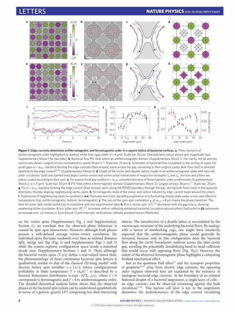
Supplementary Figure 3 – Simulations of the full model reproduce the spin-flip dynamics over long times.Frames of a simulation using parameter values at w = 4µm from the reconstructions in Supplementary Fig. 2.Top row: staggered vortex spins, corresponding to multiplying each spin site alternately by ±1 to show coherentantiferromagnetic domains as single colours. Bottom row: unstaggered vortex spins. Domain fluctuations andlarge-scale spin flips can be seen over the simulation at times extending to an equivalent of double or triple thelengths of typical observations.

equipment data capacity. In particular, the simulations exhibit domain fluctuations and spin flippingas observed in the experiments (Supplementary Fig. 1c–f), while better demonstrating the system fullyexploring configuration space. Supplementary Fig. 3 depicts a simulation using reconstructed parametervalues at w = 4µm, firmly inside the antiferromagnetic regime, run for a length equivalent to approxi-mately 25 s of an experiment with RMS kinetic energy U = 12µms−1 (the average seen in experiments;see Methods), exhibiting dynamic configuration exploration within an equilibrium distribution favouringantiferromagnetic correlation.

4 Reduction to vortex-only model

A true Langevin equation for V can be obtained by integrating Eq. (3) for P as a function of V andback-substituting2,3. Since Eq. (3) is linear in P, we have

Pi(t) = Pi(0)e−apt + Jp

!

j:Vj∼Pi

" t

0Vj(s)e

ap(s−t) ds+#

2Tp

" t

0eap(s−t) dW (s),

where the third term is an integral with respect to the standard Brownian motion W (t). When apt ≫ 1,the first term decays and the second can be approximated by pulling out Vj(s) at s = t (provided Vvaries sufficiently slowly over short time intervals), giving

Pi(t) ≈Jpap

!

j:Vj∼Pi

Vj(t) +#

2Tp

" t

0eap(s−t) dW (s). (S5)

This is valid here since ap ∼ 1 (Supplementary Fig. 2) and each 10 s experimental movie reachesnon-dimensional times t = (10 s)/τ ∼ 100. Thus Pi reduces to time-autocorrelated noise ν(t) =#

2Tp$ t0 e

ap(s−t) dW (s) about a mean proportional to the average spin of adjacent vortices [Pi]V =14

%j:Vj∼Pi

Vj ; that is, Pi ≈ (4Jp/ap)[Pi]V + ν. The noise has autocorrelation

C(t, t′) = E&ν(t)ν(t′)

'=

Tp

ap

(e−ap|t−t′| − e−ap(t+t′)

)≈ Tp

ape−ap|t−t′|

for apt, apt′ ≫ 1. In this limit, C decays rapidly away from t = t′, and ν(t) is approximately normallydistributed at every t with variance Tp/ap.

5



6

Supplementary Figure 2 – Parameters in the full model can be inferred using regression methods. Points areaverages within non-overlapping 2.5µm bins of parameters inferred for each experiment using linear regressionon a discretization of Eqs. (2) and (3), and lines are parametric best fits of selected functional forms to the points(Sec. 2).

fitted with chosen functional forms: Jv, Jp, ap with a logistic function α1+α2/(1+10α3(α4−w)); av, bvwith a rational function α1/(w+α2); and Tv, Tp with a rational function (α1+α2w)/(w2+α3w+α4)(Supplementary Fig. 2, lines). These forms were chosen as appearing to give the best representationof the data points’ behaviour (such as not introducing maxima where none are observed for Jv, Jp, ap,and not presuming too detailed a functional form for the noisiest parameters av and bv) with the fewestpossible fit parameters.

3.2 Simulation method

We numerically integrated Eqs. (2) and (3) using the discretization in Eqs. (S1) and (S2), wherein weset N = 6 and δt = 1/600 (equivalent to 1/60 s when U = 10µm). We initialized V and P to zero,and after an equilibration period of 50/δt frames we recorded every frame. Trial and error showedan observation period of 8000/δt frames in an ensemble of 25 identical repetitions to be sufficient toobtain a stable estimate of the average vortex–vortex correlation χ. This was evaluated at each of 101regularly-spaced values of w in the range minwi ≤ w ≤ maxwi (Fig. 1j).

In all simulations we use free boundary conditions (that is, setting components of P and V to zerooutside of the simulation domain) consistent with the conditions used in parameter inference. Becauseof the small size of the system being simulated, periodic boundary conditions are inappropriate as theyhave too great a dynamical influence and do not reproduce the expected spin–spin correlation behaviour.Simulations on moderately larger lattices with free boundary conditions retain the same form of cor-relation curve as for the 6 × 6 grid, but as the number of grid points increases, the antiferromagneticphase eventually disappears. This reflects the sensitivity of the system to fluctuations as vortex and pil-lar interactions compete near to a critical point; were experiments to be performed on larger lattices andparameters inferred from that data, this regime would reappear in simulations.

3.3 Spin fluctuations

As in the experiments, after equilibrating during the burn-in period, each simulation explores configura-tion space within the statistical steady state. The simulations then allow us to examine system behaviourover time scales longer than those of the experimental movies, whose durations were constrained by

4

cw

ccw1

0

-1

Vorte

x sp

in

1

0

-1Stag

gere

dvo

rtex

spin

t = 50 t = 100 t = 150 t = 200 t = 250 t = 300

Supplementary Figure 3 – Simulations of the full model reproduce the spin-flip dynamics over long times.Frames of a simulation using parameter values at w = 4µm from the reconstructions in Supplementary Fig. 2.Top row: staggered vortex spins, corresponding to multiplying each spin site alternately by ±1 to show coherentantiferromagnetic domains as single colours. Bottom row: unstaggered vortex spins. Domain fluctuations andlarge-scale spin flips can be seen over the simulation at times extending to an equivalent of double or triple thelengths of typical observations.

equipment data capacity. In particular, the simulations exhibit domain fluctuations and spin flippingas observed in the experiments (Supplementary Fig. 1c–f), while better demonstrating the system fullyexploring configuration space. Supplementary Fig. 3 depicts a simulation using reconstructed parametervalues at w = 4µm, firmly inside the antiferromagnetic regime, run for a length equivalent to approxi-mately 25 s of an experiment with RMS kinetic energy U = 12µms−1 (the average seen in experiments;see Methods), exhibiting dynamic configuration exploration within an equilibrium distribution favouringantiferromagnetic correlation.

4 Reduction to vortex-only model

A true Langevin equation for V can be obtained by integrating Eq. (3) for P as a function of V andback-substituting2,3. Since Eq. (3) is linear in P, we have

Pi(t) = Pi(0)e−apt + Jp

!

j:Vj∼Pi

" t

0Vj(s)e

ap(s−t) ds+#

2Tp

" t

0eap(s−t) dW (s),

where the third term is an integral with respect to the standard Brownian motion W (t). When apt ≫ 1,the first term decays and the second can be approximated by pulling out Vj(s) at s = t (provided Vvaries sufficiently slowly over short time intervals), giving

Pi(t) ≈Jpap

!

j:Vj∼Pi

Vj(t) +#

2Tp

" t

0eap(s−t) dW (s). (S5)

This is valid here since ap ∼ 1 (Supplementary Fig. 2) and each 10 s experimental movie reachesnon-dimensional times t = (10 s)/τ ∼ 100. Thus Pi reduces to time-autocorrelated noise ν(t) =#2Tp

$ t0 e

ap(s−t) dW (s) about a mean proportional to the average spin of adjacent vortices [Pi]V =14

%j:Vj∼Pi

Vj ; that is, Pi ≈ (4Jp/ap)[Pi]V + ν. The noise has autocorrelation

C(t, t′) = E&ν(t)ν(t′)

'=

Tp

ap

(e−ap|t−t′| − e−ap(t+t′)

)≈ Tp

ape−ap|t−t′|

for apt, apt′ ≫ 1. In this limit, C decays rapidly away from t = t′, and ν(t) is approximately normallydistributed at every t with variance Tp/ap.

5



6

-0.4 -0.2 0 0.2 0.4Mean spin of adjacent vortices

Pill

ar s

pin

-0.4

-0.2

0

0.2

0.4

-0.4 0-0.8 0.4Mean spin of adjacent vortices

Pill

ar s

pin

-0.4

-0.2

0

0.2

0.4

-0.4 0 0.80.4Mean spin of adjacent vortices

Pill

ar s

pin

-0.4

-0.2

0

0.2

c

ba

d

0 5 10 15 20 25Gap width (μm)

0.3

0.5

0.6

Pill

ar to

vor

tex

spin

ratio

ba c

0.4

Freq

uenc

y

20

40

80

0

60

100 Supplementary Figure 4 – Pillar spin distribu-tions vary linearly with the average spin of ad-jacent vortices. a–c, Two-dimensional histogramof (Pi, [Pi]V ) from three example movies, show-ing uniform spread about a line Pi ∝ [Pi]V . Gapwidths 7, 10 and 18µm, respectively. d, The pro-portionality constant α, where Pi ≈ −α[Pi]V , de-pends weakly on gap width. Direct correlationsfrom data (blue circles) compare well with the theo-retical result α = −4Jp/ap calculated with inferredmodel parameters (red diamonds). Each point rep-resents an average over ≥ 5 movies in 3µm binsat 1.5µm intervals; vertical bars indicate standarderrors (Methods).

Now, in Eq. (2), interaction with P arises through the term Jp∑

j:Pj∼ViPj in ∂H/∂Vi. By Eq. (S5),

this approximates to

Jp∑

j:Pj∼Vi

Pj ≈J2p

ap

⎡

⎣4Vi + 2∑

j:Vj∼Vi

Vj + (n.n.n.)

⎤

⎦+ Jp

4∑

j=1

ν(j), (S6)

where ν(j) are i.i.d. noise processes as above, and ‘n.n.n.’ denotes next-nearest-neighbour interactionswhich we neglect. When substituted into Eq. (2), each noise term contributes Jpν(j)dt, which representsa contribution of the form Jp

∫ t0 ν

(j)(s) ds in the formal integral representation of Eq. (2). Inserting thedefinition of ν into this integral and exchanging the order of integration implies

Jp

∫ t

0ν(j)(s) ds =

Jp√

2Tp

ap

∫ t

0[1− eap(s−t)] dW (s).

In our experiments, we found |Jp/ap| ≈ 1/10 and Tp ! Tv over all gap widths (Supplementary Fig.2), so these are weak contributions to the noise in V. Indeed, the integral has variance t − 3/(2ap) +O(e−apt) as t → ∞, so for large ap its effect can be approximated by the pure Brownian motion∫ t0 dW (r) (whose variance is t). Thus the contributions Jpν(j)dt reduce to small Brownian noise terms(Jp

√2Tp/ap)dW , which combine with the existing noise into one single term

√2TdW of slightly

increased temperature T = Tv + 4TpJ2p/a

2p. Substituting Eq. (S6) into Eq. (2) yields new approximate

V dynamics obeying dV = −(∂H/∂V)dt+√2TdW with effective Hamiltonian

H(V) = −J∑

Vi∼Vj

ViVj +∑

Vi

(12aV

2i + 1

4bV4i

),

where the effective coupling constants are J = Jv + 2J2p/ap, a = av − 4J2

p/ap and b = bv.Though this reduction will only be achieved exactly in the thermodynamic limit when boundary ef-

fects are eliminated, this still serves as a good approximation for a finite system. To verify this reductionwith our experimental data, we compared Pi with [Pi]V . Consistent with Eq. (S5), we found Pi to belinearly correlated with [Pi]V in every square-lattice experiment (Supplementary Fig. 4a–c), confirmingour use of a quadratic potential for P. Writing −α for the correlation coefficient, we found α ≈ 0.5with weak dependence on the gap width; this compares well with the analytic result α = −4Jp/ap fromEq. (S5) when calculated using experimentally inferred parameters (Supplementary Fig. 4d).

6



6

Supplementary Figure 4 – Pillar spin distribu-tions vary linearly with the average spin of ad-jacent vortices. a–c, Two-dimensional histogramof (Pi, [Pi]V ) from three example movies, show-ing uniform spread about a line Pi ∝ [Pi]V . Gapwidths 7, 10 and 18µm, respectively. d, The pro-portionality constant α, where Pi ≈ −α[Pi]V , de-pends weakly on gap width. Direct correlationsfrom data (blue circles) compare well with the theo-retical result α = −4Jp/ap calculated with inferredmodel parameters (red diamonds). Each point rep-resents an average over ≥ 5 movies in 3µm binsat 1.5µm intervals; vertical bars indicate standarderrors (Methods).

Now, in Eq. (2), interaction with P arises through the term Jp∑

j:Pj∼ViPj in ∂H/∂Vi. By Eq. (S5),

this approximates to

Jp∑

j:Pj∼Vi

Pj ≈J2p

ap

⎡

⎣4Vi + 2∑

j:Vj∼Vi

Vj + (n.n.n.)

⎤

⎦+ Jp

4∑

j=1

ν(j), (S6)

where ν(j) are i.i.d. noise processes as above, and ‘n.n.n.’ denotes next-nearest-neighbour interactionswhich we neglect. When substituted into Eq. (2), each noise term contributes Jpν(j)dt, which representsa contribution of the form Jp

∫ t0 ν

(j)(s) ds in the formal integral representation of Eq. (2). Inserting thedefinition of ν into this integral and exchanging the order of integration implies

Jp

∫ t

0ν(j)(s) ds =

Jp√

2Tp

ap

∫ t

0[1− eap(s−t)] dW (s).

In our experiments, we found |Jp/ap| ≈ 1/10 and Tp ! Tv over all gap widths (Supplementary Fig.2), so these are weak contributions to the noise in V. Indeed, the integral has variance t − 3/(2ap) +O(e−apt) as t → ∞, so for large ap its effect can be approximated by the pure Brownian motion∫ t0 dW (r) (whose variance is t). Thus the contributions Jpν(j)dt reduce to small Brownian noise terms(Jp

√2Tp/ap)dW , which combine with the existing noise into one single term

√2TdW of slightly

increased temperature T = Tv + 4TpJ2p/a

2p. Substituting Eq. (S6) into Eq. (2) yields new approximate

V dynamics obeying dV = −(∂H/∂V)dt+√2TdW with effective Hamiltonian

H(V) = −J∑

Vi∼Vj

ViVj +∑

Vi

(12aV

2i + 1

4bV4i

),

where the effective coupling constants are J = Jv + 2J2p/ap, a = av − 4J2

p/ap and b = bv.Though this reduction will only be achieved exactly in the thermodynamic limit when boundary ef-

fects are eliminated, this still serves as a good approximation for a finite system. To verify this reductionwith our experimental data, we compared Pi with [Pi]V . Consistent with Eq. (S5), we found Pi to belinearly correlated with [Pi]V in every square-lattice experiment (Supplementary Fig. 4a–c), confirmingour use of a quadratic potential for P. Writing −α for the correlation coefficient, we found α ≈ 0.5with weak dependence on the gap width; this compares well with the analytic result α = −4Jp/ap fromEq. (S5) when calculated using experimentally inferred parameters (Supplementary Fig. 4d).

6

0

1

0.5

Mea

n ad

jace

nt v

orte

x sp

in

0

1

0.5

Mea

n ad

jace

nt v

orte

x sp

in

-1.5 -1 -0.5 0 0.5 1.51-3

-2

-1

0

1

3

2

Vortex spin

Veffanti

-1.5 -1 -0.5 0 0.5 1.51Vortex spin

-3

-2

-1

0

1

3

2

Veffanti

a b c

-1.5 -1 -0.5 0 0.5 1.51Vortex spin

-3

-2

-1

0

1

3

2

Veffanti

-1.5 -1 -0.5 0 0.5 1.51Vortex spin

2

4

6

0

-2

Veffsym

-1.5 -1 -0.5 0 0.5 1.51Vortex spin

2

4

6

0

-2

Veffsym

d e f

-1.5 -1 -0.5 0 0.5 1.51Vortex spin

2

4

6

0

-2

Veffsym

Supplementary Figure 5 – Parameters in the reduced model can be inferred by fitting effective single-spinpotentials. Reduced model parameters βJ , βa and βb are estimated by fitting the antisymmetric and symmetricparts of the effective potential Veff(Vi | [Vi]V ) (Sec. 5.1). Data shown from three example movies of square latticeswith gap widths 7µm (a,d), 10µm (b,e) and 18µm (c,f). a–c, The antisymmetric part of the effective potentialreveals the vortex–vortex coupling βJ , spanning the range J < 0 (a), J ≈ 0 (b) and J > 0 (c). Estimated Veff

anti

(points), coloured by mean adjacent spin [Vi]V . d–f, The symmetric part of the effective potential reveals thenon-interacting single-spin potential, which flattens with increasing gap width. Estimated Veff

sym (points) colouredby mean adjacent spin [Vi]V , with fitted single-spin potentials (lines).

5 Parameter inference under the reduced model

5.1 Distribution fitting

We assume that V obeys a Boltzmann distribution p(V) ∝ e−βH(V). The probability density p(Vi | [Vi]V )of one spin Vi conditional on the mean of its adjacent spins [Vi]V = 1

4

!j :Vj∼Vi

Vj satisfies

log p(Vi | [Vi]V )− log p(0 | [Vi]V ) = −Veff(Vi | [Vi]V ), (S7)

where we have defined the effective single-vortex potential

Veff(Vi | [Vi]V ) = −4βJVi[Vi]V + 12βaV

2i + 1

4βbV4i .

We estimate p(Vi | [Vi]V ) for each movie by forming a two-dimensional histogram in Vi and [Vi]V andthen normalizing at every fixed Vi. In forming the histogram, we exploit the invariance of Veff under thetransformation Vi → −Vi and [Vi]V → −[Vi]V to double the number of data points.

Taking the antisymmetric part Veffanti = 1

2

"Veff(Vi | [Vi]V )− Veff(−Vi | [Vi]V )

#eliminates the non-

interacting terms, so Eq. (S7) implies

12 [− log p(Vi | [Vi]V ) + log p(−Vi | [Vi]V )] = −4βJVi[Vi]V .

This allows estimation of the interaction constant βJ from the density p(Vi|[Vi]V ) (Fig. 2a and Supple-mentary Fig. 5a–c). The symmetric part Veff

sym = 12

"Veff(Vi | [Vi]V ) + Veff(−Vi | [Vi]V )

#eliminates the

interaction term in a similar fashion, so Eq. (S7) now implies

1

2[− log p(Vi | [Vi]V )− log p(−Vi | [Vi]V )] + log p(0 | [Vi]V ) =

1

2βaV 2

i +1

4βbV 4

i .



6

Typically there are fewer observations near Vi = 0, so p(0 | [Vi]V ) can be difficult to infer directly. In-stead, we adjust log p(0 | [Vi]V ) for each [Vi]V bin to minimize the difference between Veff

sym(V | [Vi]V )

and Veffsym(V | 0). We then fit the remaining single vortex potential with parameters βa and βb (Supple-

mentary Fig. 5d–f), from which we compute the spins ±Vmin (Vmin > 0) minimizing the local effectivesingle-spin energy Veff

sym, namely

Vmin =

{√|a|/b if a < 0,

0 if a > 0,

and the effective spin-flip energy barrier

Veffsym(0)− Veff

sym(±Vmin) =

{βa2/(4b) if a < 0,

0 if a > 0,

which together characterize the single-spin symmetric quartic potential (Fig. 2b,c).To ensure boundary conditions do not have a strong effect on the inferred parameters by compar-

ison with those used in the SDE discretization method (see below), boundary terms are treated in thismethod using neighbour averaging whereby the mean adjacent spin [Vi]V is computed as an averageover only two spins (in a corner) or three spins (at an edge). This corresponds to assuming that, in eachcomputation of [Vi]V , spin sites absent from the lattice are the mean of the sites present in the sum.

5.2 SDE discretization

Estimations made by the above method were verified by estimations obtained through the same SDE dis-cretization method used in the full model. Though the absence of pillars now means periodic boundaryconditions could be used, we retain the free boundary conditions to maintain consistency with the fullmodel and for comparison with the averaging conditions used above. The components of the reducedmodel SDE dV = −(∂H/∂V)dt+

√2TdW have Euler–Maruyama discretization

Vi(t+ δt) = (1− aδt)Vi(t)− bδtVi(t)3 + Jδt

∑

j :Vj∼Vi

Vj(t) +√2T δtNi,

where Ni are independent N (0, 1) random variables. Performing linear regression of Vi(t+ δt) on thethree variables

⎧⎨

⎩Vi(t), Vi(t)3,

∑

j :Vj∼Vi

Vj(t)

⎫⎬

⎭

then gives estimates {1 − aδt,−bδt, Jδt} of the respective coefficients, from which estimates a, b andJ of the variables a, b and J can be deduced. The estimate T of the fluctuation strength T is estimatedvia the variance 2T δt of the residuals to the regression, which gives an estimate β = 1/T of the inverse‘temperature’ β in the Boltzmann distribution. The non-dimensional combinations βJ , βa and βb canthen be directly compared with the estimates obtained using the distribution-fitting method.

Though SDE discretization independently gives both temperature and coupling constants, it is likelyto possess greater intrinsic bias than distribution fitting. Discretization was the only method open forthe full model, as the SDE steady state cannot be solved analytically. However, since the reduced modelallows for distribution fitting, coupling constant values obtained using that method are preferable, withSDE discretization functioning as an independent verification.

6 One-dimensional geometries

As well as the square and triangular lattices discussed in the main text (Figs. 1 and 3), we also per-formed experiments on lines of connected vortices (Supplementary Fig. 6). As the finite-circumference

8



6

Typically there are fewer observations near Vi = 0, so p(0 | [Vi]V ) can be difficult to infer directly. In-stead, we adjust log p(0 | [Vi]V ) for each [Vi]V bin to minimize the difference between Veff

sym(V | [Vi]V )

and Veffsym(V | 0). We then fit the remaining single vortex potential with parameters βa and βb (Supple-

mentary Fig. 5d–f), from which we compute the spins ±Vmin (Vmin > 0) minimizing the local effectivesingle-spin energy Veff

sym, namely

Vmin =

{√|a|/b if a < 0,

0 if a > 0,

and the effective spin-flip energy barrier

Veffsym(0)− Veff

sym(±Vmin) =

{βa2/(4b) if a < 0,

0 if a > 0,

which together characterize the single-spin symmetric quartic potential (Fig. 2b,c).To ensure boundary conditions do not have a strong effect on the inferred parameters by compar-

ison with those used in the SDE discretization method (see below), boundary terms are treated in thismethod using neighbour averaging whereby the mean adjacent spin [Vi]V is computed as an averageover only two spins (in a corner) or three spins (at an edge). This corresponds to assuming that, in eachcomputation of [Vi]V , spin sites absent from the lattice are the mean of the sites present in the sum.

5.2 SDE discretization

Estimations made by the above method were verified by estimations obtained through the same SDE dis-cretization method used in the full model. Though the absence of pillars now means periodic boundaryconditions could be used, we retain the free boundary conditions to maintain consistency with the fullmodel and for comparison with the averaging conditions used above. The components of the reducedmodel SDE dV = −(∂H/∂V)dt+

√2TdW have Euler–Maruyama discretization

Vi(t+ δt) = (1− aδt)Vi(t)− bδtVi(t)3 + Jδt

∑

j :Vj∼Vi

Vj(t) +√2T δtNi,

where Ni are independent N (0, 1) random variables. Performing linear regression of Vi(t+ δt) on thethree variables

⎧⎨

⎩Vi(t), Vi(t)3,

∑

j :Vj∼Vi

Vj(t)

⎫⎬

⎭

then gives estimates {1 − aδt,−bδt, Jδt} of the respective coefficients, from which estimates a, b andJ of the variables a, b and J can be deduced. The estimate T of the fluctuation strength T is estimatedvia the variance 2T δt of the residuals to the regression, which gives an estimate β = 1/T of the inverse‘temperature’ β in the Boltzmann distribution. The non-dimensional combinations βJ , βa and βb canthen be directly compared with the estimates obtained using the distribution-fitting method.

Though SDE discretization independently gives both temperature and coupling constants, it is likelyto possess greater intrinsic bias than distribution fitting. Discretization was the only method open forthe full model, as the SDE steady state cannot be solved analytically. However, since the reduced modelallows for distribution fitting, coupling constant values obtained using that method are preferable, withSDE discretization functioning as an independent verification.

6 One-dimensional geometries

As well as the square and triangular lattices discussed in the main text (Figs. 1 and 3), we also per-formed experiments on lines of connected vortices (Supplementary Fig. 6). As the finite-circumference

8

a b

c d

Spi

n-sp

in c

orre

latio

n

cb

0 20Gap width (µm)

10 4030

0

-0.5

a

-1

CW

CCW1

0

-1

orte

spi

n

Supplementary Figure 6 – One-dimensionallattices adopt antiferromagnetic states. a, Atthe smallest gap widths, vortices interact weaklyresulting in strong but randomly oriented circula-tion. Gap width 7µm. b,c, Intermediate and largegaps show strong antiferromagnetic order. Gapwidths 16 and 28µm. False colour in a–c denotesmeasured vortex spin. Scale bar: 50µm. d, Thespin–spin correlation χ shows the antiferromag-netic state to be largely favoured in lines of cav-ities. Each point represents an average over ≥ 5movies in 3µm bins at 1.5µm intervals; verticalbars indicate standard errors (Methods).

pillars are no longer present in a line of vortices, it is not clear whether the same edge-current-mediatedferromagnetism should be expected. Indeed, we did not observe significant ferromagnetic behaviour atany gap sizes (Supplementary Fig. 6d), suggesting that it is difficult to maintain the single long, uniformedge current that would be necessary for a positively-correlated state. Furthermore, experiments per-formed on isolated pairs of vortices support these results, in which 76% of the vortex pairs adopted anantiferromagnetic state (out of 34 pairs) with gap sizes between 20µm and 38µm.

7 Model generalizations

There are more general forms of the model in Eqs. (2) and (3) which preserve at least some form of localequilibrium. These add flexibility through further couplings or fields at the expense of increased com-plexity. Though we did not find a need for any further generality, they cannot necessarily be disregardeda priori, which we discuss further here.

7.1 Cross-coupled models with frictional dissipation

One generalization of Eqs. (2) and (3) is to add dissipative cross-couplings. Write X = (V,P) for theconcatenation of the vectors V and P. In this formalism, Eqs. (2) and (3) read

dXi = − ∂H

∂Xidt+

!2TidWi, (S8)

where Ti is Tv or Tp as appropriate and the Wi are uncorrelated Wiener processes as before. (Repeatedindices do not imply summation.) However, in general, we need not have diagonal coupling to deriva-tives of H . We could instead write4

dXi = −"

j

Mij∂H

∂Xjdt+

"

j

mij

!2TjdWj ,

where the Mij are the components of a more general coupling matrix, and m is the square-root matrixsuch that m2 = M. Onsager reciprocity would then demand Mij = Mji if the vortex spins and pillarflows were relaxing to a true thermodynamic equilibrium with Tv = Tp.

The simplest form of this generalization would be to posit a constant coupling between a vortexVi and the gradients ∂H/∂Pj of its neighbouring pillars Pj , plus the corresponding reverse coupling.However, a single bacterial vortex experiences most frictional dissipation against the confining upperand lower walls of the cavity, rather than against the much smaller and more porous contact area ofthe edge currents. Similarly, a single pillar edge current experiences most friction against the solid



6

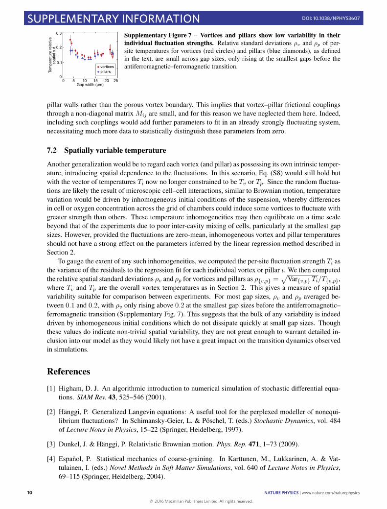
0 5 15 20 25

0.1

0.3

Tem

pera

ture

rela

tive

spat

ial s

.d.

0

Gap width (μm)

0.2

vorticespillars

10

Supplementary Figure 7 – Vortices and pillars show low variability in theirindividual fluctuation strengths. Relative standard deviations ρv and ρp of per-site temperatures for vortices (red circles) and pillars (blue diamonds), as definedin the text, are small across gap sizes, only rising at the smallest gaps before theantiferromagnetic–ferromagnetic transition.

pillar walls rather than the porous vortex boundary. This implies that vortex–pillar frictional couplingsthrough a non-diagonal matrix Mij are small, and for this reason we have neglected them here. Indeed,including such couplings would add further parameters to fit in an already strongly fluctuating system,necessitating much more data to statistically distinguish these parameters from zero.

7.2 Spatially variable temperature

Another generalization would be to regard each vortex (and pillar) as possessing its own intrinsic temper-ature, introducing spatial dependence to the fluctuations. In this scenario, Eq. (S8) would still hold butwith the vector of temperatures Ti now no longer constrained to be Tv or Tp. Since the random fluctua-tions are likely the result of microscopic cell–cell interactions, similar to Brownian motion, temperaturevariation would be driven by inhomogeneous initial conditions of the suspension, whereby differencesin cell or oxygen concentration across the grid of chambers could induce some vortices to fluctuate withgreater strength than others. These temperature inhomogeneities may then equilibrate on a time scalebeyond that of the experiments due to poor inter-cavity mixing of cells, particularly at the smallest gapsizes. However, provided the fluctuations are zero-mean, inhomogeneous vortex and pillar temperaturesshould not have a strong effect on the parameters inferred by the linear regression method described inSection 2.

To gauge the extent of any such inhomogeneities, we computed the per-site fluctuation strength Ti asthe variance of the residuals to the regression fit for each individual vortex or pillar i. We then computedthe relative spatial standard deviations ρv and ρp for vortices and pillars as ρ{v,p} =

!Var{v,p} Ti/T{v,p},

where Tv and Tp are the overall vortex temperatures as in Section 2. This gives a measure of spatialvariability suitable for comparison between experiments. For most gap sizes, ρv and ρp averaged be-tween 0.1 and 0.2, with ρv only rising above 0.2 at the smallest gap sizes before the antiferromagnetic–ferromagnetic transition (Supplementary Fig. 7). This suggests that the bulk of any variability is indeeddriven by inhomogeneous initial conditions which do not dissipate quickly at small gap sizes. Thoughthese values do indicate non-trivial spatial variability, they are not great enough to warrant detailed in-clusion into our model as they would likely not have a great impact on the transition dynamics observedin simulations.

References

[1] Higham, D. J. An algorithmic introduction to numerical simulation of stochastic differential equa-tions. SIAM Rev. 43, 525–546 (2001).

[2] Hanggi, P. Generalized Langevin equations: A useful tool for the perplexed modeller of nonequi-librium fluctuations? In Schimansky-Geier, L. & Poschel, T. (eds.) Stochastic Dynamics, vol. 484of Lecture Notes in Physics, 15–22 (Springer, Heidelberg, 1997).

[3] Dunkel, J. & Hanggi, P. Relativistic Brownian motion. Phys. Rep. 471, 1–73 (2009).

[4] Espanol, P. Statistical mechanics of coarse-graining. In Karttunen, M., Lukkarinen, A. & Vat-tulainen, I. (eds.) Novel Methods in Soft Matter Simulations, vol. 640 of Lecture Notes in Physics,69–115 (Springer, Heidelberg, 2004).

10



6

ferromagnetic and antiferromagnetic order in bacterial ...dunkel/papers/2016wietal_natphys.pdf ·...

Documents