fertility and mortality estimation using model stable age distributions

FERTILITY AND MORTALITY ESTIMATION USING MODEL STABLE AGE DISTRIBUTIONS

A. BACKGROUND OF METHODS

1. Gcnerdprinci@es underlying the use of model stable populat~onr for estimation purposes

Lotkai proved that the age distribution of any population that is subject, for a sufficiently long time, to constant fertility and mortality becomes fixed. He called this end-product of constant demographic conditions a "stable population", characterized both by an unchang- ing age distribution and by a fixed annual rate of natural increase.

The age distribution of a stable population is jointly determined by the mortality schedule (that is, by the life table) to which the population has been subject and by its annual rate of growth. In chapter I, section C, the equation defining the density function determining the age distribution of a stable population was presented. It has the form

where c(x) is the infinitesimal proportion of the stable population at exact age x ; b is the constant birth rate; r is the constant rate of natural increase; and I(x) is the probability of surviving from birth to age x (that is, it is the usual life table function with an l(0) radix of 1.0).

The usefulness of model stable populations in estimating the parameters determining the growth and structure of actual populations derives from three considerations. First, it has been found that for a population in which fertility has been approximately constant and in which mortality has recently undergone a steady reduction, the age distribution closely resembles that of a stable population generated by equation (A.l), with l(x) being the probability of survival to age x in the current life table and r being the current rate of increase. Secondly, these conditions (the recent course of fertility approximately constant and mortality either approximately constant or recently declining) are, or have until recently been, characteristic of the population of many developing countries. Thirdly, the availability of fairly flexible sets of model stable populations, such as those generated on the basis of the ~ o a l e - ~ e m e n q life tables with a range

l~ l fred J. Lotka and F. R. Sharpe, "A problem in a e distribution'', Philosophicul Mugazine, vol. 2 I . N o I24 (April lh ;). pp. 435-438.

Andey J. Code and Paul Demeny. Regional Model Lifc Tables and St& Popu/utiom (Princeton, New Jersey. Princeton Un~venity Press. 1 %6).

of growth rates, makes it possible to identify with rela- tive ease a stable age distribution approximating a reported age distribution in an actual application. The underlying characteristics of the stable population can then be adopted as estimates of the demographic parameters of the population being studied.

Useful estimates can be made by selecting a model stable population matching two characteristics, presumed to have been accurately recorded .or estimated, of the reported population. In the Coale- Demeny system, a model stable population within each family is fully determined by the level of mortality and the growth rate; thus, two parameters are sufficient to identify a stable population within a given family. For example, the reported proportion under any given age, in conjunction with any one of the following parameters-an estimated 1 (x) for any age x , the rate of increase or the population death rate-uniquely determines a model stable population, provided that a specific pattern of mortality has been deemed an appropriate representation of that experienced in reality.

When a model stable population has been identified, selected characteristics of the stable population serve as estimates of the corresponding characteristics of the population in question. For example, the birth rate in a given pppulation can be estimated by identifying a model stable population in which the probability of surviving from'birth to age 5, 1(5), and the proportion under age I5 are the same as those in the given population. The birth rate in the stable population is then taken as an estimate of the actual birth rate.

The value of estimates based on fitting model stable populations is limited by a number of practical considerations. First, no actual population is genuinely stable. Fertility may vary as a result of recent trends or because of special past episodes, such as wars or epi- demics. Age-selective and sex-selective migration can affect both the rate of growth and the age distribution of the population, and the recent mortality declines observed in many countries produce age distributions that do not conform exactly to those predicted by the equation defining a stable population. Secondly, the characteristics of the population being studied that are available to identify a model stable population are often imprecisely recorded (the age distribution is distorted by differential omission by age, or the intercensal rate of increase calculated from census counts at two points in time is biased because of differential completeness of coverage between the two censuses). Lastly, the esti-

mates of a certain parameter (the birth rate, for example) obtained by using different sets of model stable populations (such as those generated by the different mortality families of the Coale-Demeny set) may be quite different. In most cases, there is uncertainty about which mortality pattern approximates most closely that experienced by a given population; and since the number of model families is limited, there is no guarantee that they cover all possible experience, so the accuracy of the estimates obtained may often be question- able. In this respect, it is appropriate to mention that the availability of the United Nations model life tables for developing countries,' in conjunction with stable populations generated by them: will substantially enhance the estimation capabilities by expanding the spectrum of models from which one can choose.

Ideally, the estimates derived by fitting a model stable population to a reported age distribution should be insensitive to the practical difficulties mentioned above. Therefore, they should not be much affected by the deviations from stability most commonly encountered in practice. To achieve this end, the fitted stable population should be identified on the basis of parameters for which estimates are least likely to be biased by the usual data flaws (such as age-misreporting) and which should assume much the same values whichever set of model stable populations is employed to derive them. (In this chapter, only stable populations based on the four Coale-Demeny families are used, so this last desirable

' M o d ti l Tables or lkvcloping Countries (United Nations publi- cation, Sales 4 o. E.81. 4 111.7). ' S1461C P o ~ i o n s Cornspondin to the New United Natiom Mo&l

ti@ T ~ S ~ W wWg ~ t t m s &T/ES*/SER.R N().

feature will at most be satisfied with respact to variations between these four models.)

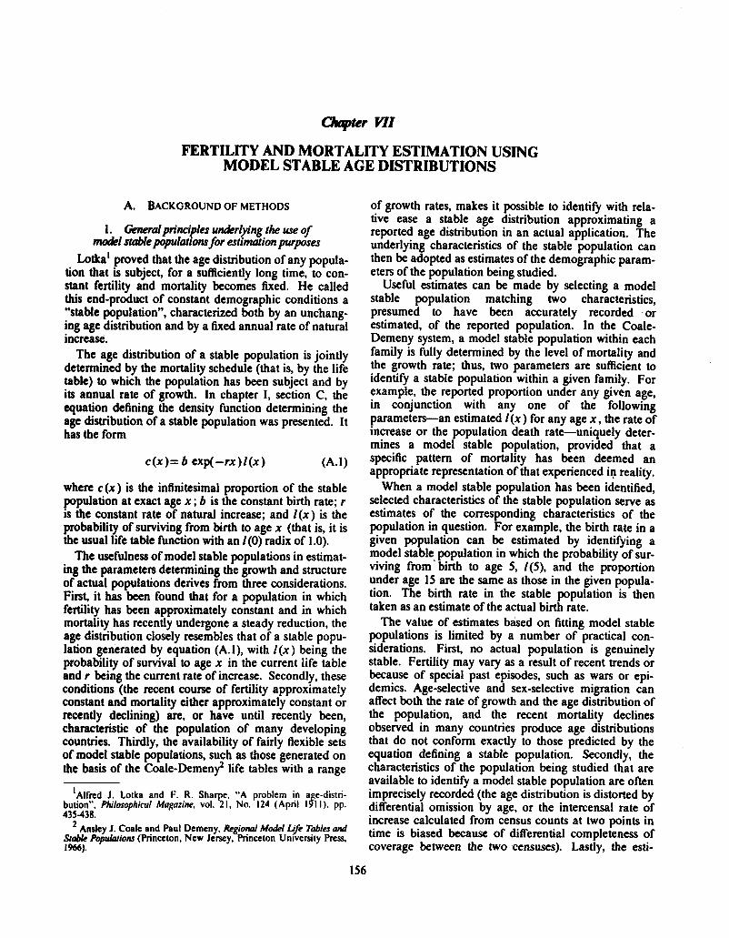
Experience has shown that the most efficient use of stable populations requires the identification not of one single stable population from which all parameters are derived, but rather of a number of stable populations identified by using different pairs of reported values and applied to estimate different sets of underlying parameters. For example, it is often the case that the best estimate of fertility in the population under review (meas- ured as the birth rate or as total fertility) may be obtained by selecting the model stable population that matches the value of Z(5) and the proportion of the population of both sexes under age 15; while in order to estimate mortality levels over age 5, a model stable population should be fitted on the basis of the estimated growth rate and the proportion of the population under age 15. Surprisingly enough, some of the estimates derived from a model stable population by using the first of these strategies are quite accurate even when the population in question is very far from being stable. As examples, table 141 shows the estimated birth rates obtained by fitting a stable population, on the basis of the reported proportion under age 15 for both sexes combined, Z(5) and the growth rate, to populations that, as in the case of Sweden, cannot be considered even remotely stable since they have experienced substantial declines both in fertility and in mortality. For comparison, table 141 also displays estimates of the birth rate derived from registered births (in all the countries considered, birth registration is virtually complete). The coincidence between the two sets of estimates is reassur- ing.

2. Ogmmuzation of this chapter Essentially, only two methods of estimation using

TABLE 141. ESTIMATION OF AVERAGE BIRTH RATE OVER THE 15-YEAR PERIOD PRECEDING ENUMERATION FROM THE PROPORtlON OF THE POPULATION UNDER AGE 15. C(I5). THE PROBABILITY OF SURVIVING TO AGE 5. I($). AND THE CONSTANT R A ~ OF NATURAL INCREASE. r . FOR SELECTED NON-STABLE POPULA~ONS

A ~ w m I r M I l g I h e I J ~ ~ ~ m

lnumnrd

P2 J-ol "%mznkw - * mA2F "r;;" 5- (3) (4) (5)

(a) Swviwrship pmbability estimated from &a on chilokn e w borrp M d d v i n g for nvmen aged 30-34

..................... Belgium 1961-1970 Dec. 1970 0.0 163 0.0167 Bulgaria ..................... 1956-1965 Dec. 1965 0.0184 0.0 180

................. C~sta Rica 1963-1973 Mar. 1973 0.0406 0.04 17 Poland ........................ 1960-1970 Dec. 1970 0.0202 0.0 199 Y ugdavia ................. 1961-1971 Mar. 1971 0.02 15 0.02 13

(b) Surviwnhip probability obtained from published life tables cornsponding to about 7.5 yrars befom enumeration

............... Hong Kong 1960-1971 Mar. 1971 0.0302 0.0295 Japan ......................... 1950-1%5 Oct. 1965 0.0 190 0.01%

............... Netherlands 1918.1922- , 1933-1937 1933-1937 0.0235 0.0238

Sweden ...................... 1798- 1802- 1833- 1837 1813-1817 0.03 19 0.03 13

Sweden ...................... 1918-1922: 1933-1937 1933-1937 0.0167 0.0167

Sweden ...................... 194-1965 1965 0.0148 0.0 1 50

model stable populations are presented in this chapter. Experience has shown that these variants of the more general procedures described in a United Nations manual5 are more likely to yield acceptable parameter estimates in populations that are not truly stable (because of recent changes in mortality) or whose basic data are distorted by reporting errors. Model stable populations can also be used to assass the extent of such errors and to identify typical distortion patterns in

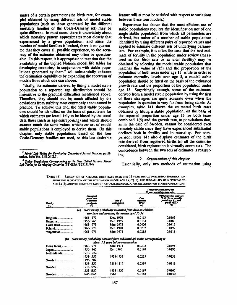
reported age distributions; and because it is important to explore the quality of the available data before any estimation method is applied, one of the sections that follows is devoted to the description of a simple procedure that allows the assessment of age distributions. To guide the reader in the use of this chapter, the contents of the sections are briefly described below (table 142 presents the data requirements of, and the parameters estimated by, the methods suggested):

TABLE 142. SCHEMATIC GUIDE TO CONT ENfS OF CHAFTER VII

*PI011

B. Evaluation of age distributions

C. Estimation of fertility from the proportion of the population under age I5 and the probability of surviving to age 5

D. Estimation of the expectation of life at age 5 and of the death rate over age 5 from the proportion under age I5 and the rate of increase

W 6 W h Population classified by five-year age

group and by sex

Population classified by five-year age group (and by sex, if available)

An estimate of 1(5), the probability of surviving from birth to age 5, for both sexes and referring to the mid- dle of the 15-year period preceding enumeration

m-P-'--J Assessment of data quality, with par-

ticular emphasis on age-reporting

Average birth rate over the 15-year period preceding enumeration

Average total fertility during the same period

Average gross reproduction rate during the same period

Population classified by five-year age Adjusted estimate of the birth rate group

An estimate of the growth rate for the 15-year period preceding enumeration

An estimate of l(5) for both sexes. referring roughly to the mid-point of the 15-year period precedihg enumeration

Population classified by five-year age Expectation of life over age 5 group and by sex Death rate over age 5

An estimate of the rate of natural in- A life table over age 5 crease for the period preceding enumeration (usually obtained from census counts at two points in time)

Section B. Evaluation of age distributions. This section presents a simple procedure for assessing the quality of a reported age distribution and its similarity to that of a truly stable population;

Section C. Estimation of fertility from the proportion of the population under age 15 and the probability of surviving to age 5. This section presents a method that allows the estimation of the birth rate and of total fertility by fitting a stable population on the basis of the reported proportion under age 15 for both sexes, denoted by C(15), and an estimate of 1(5), the probability of surviving from birth to age 5, also for both sexes;

Secrion D. Estimation of the expectation of life at age 5 and of the death rate over age 5 from the proportion u d r

Manual IY: Methocir o Ertimaring Basic Demographic Memures

E.67.XIII.2). J fnun Incomplere Doro ( nited Natlons publicat~on, Sales No.

age 15 and the rate of increase. This section presents a method that allows the estimation of mortality over age 5 by fitting a stable population on the basis of the reported proportion under age 15 for both sexes, C(15), and an estimate of the rate of natural increase, r , of the entire population.

B. EVALUATION OF AGE DISTRIBUTIONS

1. h i s of method and its rationale Knowledge of the population classified by age and

sex, that is, the population age distribution, is generally a starting-point in identifying an appropriate model stable population. Because of major errors that may be present in the recorded age distribution, it is not always easy to select a model stable population that best fits the underlying true age distribution, even when that distribution is very close to being genuinely stable.

There are two main causes of error in age distributions: the selective omission of persons of a given age; and the misreporting of age of those counted. Very often, it is impossible to distinguish the magnitude of each of these two types of error, since their effects are similar. For example, a deficit of persons in a certain age group may be caused by their total omission or by their transference to other age groups, or by both factors combined. Age-misreporting is generally the most pre- valent error in age distributions, but differential coverage by age and sex is also a likely cause of some distortions for particular age ranges.

Misclassification of the enumerated population according to age is often due to defective age-reporting by its members (or to defective estimation of age by interviewers). A very common type of age-misreporting is known as "age-heaping", which consists of the tendency on the part of respondents or interviewers to "round" the reported age to a slightly different age ending in some preferred digit. In practice, ages ending with zero or five are usually preferred over other endings (one or nine, for example), so age distributions by single years of age often exhibit peaks at ages 20,25,30 and so on, while troughs are associated with ages 29,3 1,39,4 1, etc. If, for cultural reasons, some other ages are important to the population in question, they may also attract more respondents than would be expected. Thus, it is

b frequently found that age 12 is more attractive than either age 10 or age 15.

Age-heaping is reduced when age can be ascertained by means of a question about date of birth rather than about age itself. Respondents are less likely to round year of birth than age, although interviewers, when assigning ages in cases of uncertainty, may mix the rounding of the year of birth with the translation of rounded ages into years of birth. In addition, some heaping on years of birth ending in preferred digits may be expected; and the analyst must bear this possibility in mind as its age pattern may not resemble that of conventional age-heaping. Furthermore, this method of inves- tigating age (through date of birth) only performs better than a direct question on age if most members of the population know their date of birth (an age distribution based on dates of birth may exhibit less heaping than one based on information about age but be no more accurate on an overall basis). In countries where a size- able proportion of the population is illiterate and where the reckoning of age is traditionally not important, the use of a question on age may be equally appropriate, since often the respondents will not--or cannot-supply a year of birth or even an age, which must therefore be estimated by the interviewer.

When an age distribution by single year of age is available, the incidence of age-heaping can be easily ascertained by plotting the numbers observed at each age. If age-reporting were perfect and there were no omission, the age distribution would approximate a smooth curve, disturbed only by genuinely large or small cohorts resulting from wars or other episodes caus- ing sharp fluctuations in the birth rate or in infant mor-

tality. However, such genuine fluctuations will not recur at the same digits in the successive age decades.

Because most age distributions are more or less affected by heaping, the use of data classified by single year of age is not recommended for most demographic analysis. Rather, cumulated data should be used, since cumulation reduces the effects of heaping and other forms of age-misreporting. The most common form of cumulation is a five-year group, which, though less sensitive to heaping than a single-year group, is still quite affected by transfers into and out of each age group. For most countries, a graph of the numbers observed within each five-year age group, though less ragged than the plot of the age distribution by single years, still exhi- bits marked irregularities.

A better way of reducing the effects of heaping, and of age-misreporting in general, is to cumulate from age. zero to age x (usually a multiple of five); or, equivalently, from age x to the upper age-limit of the population, o. Age groups of this type are affected only by transfers across their only boundary (age x ) and therefore introduce a strong smoothing element. Because of their robustness to age-misreporting, this type of age group is used when identifying a best fitting stable population.

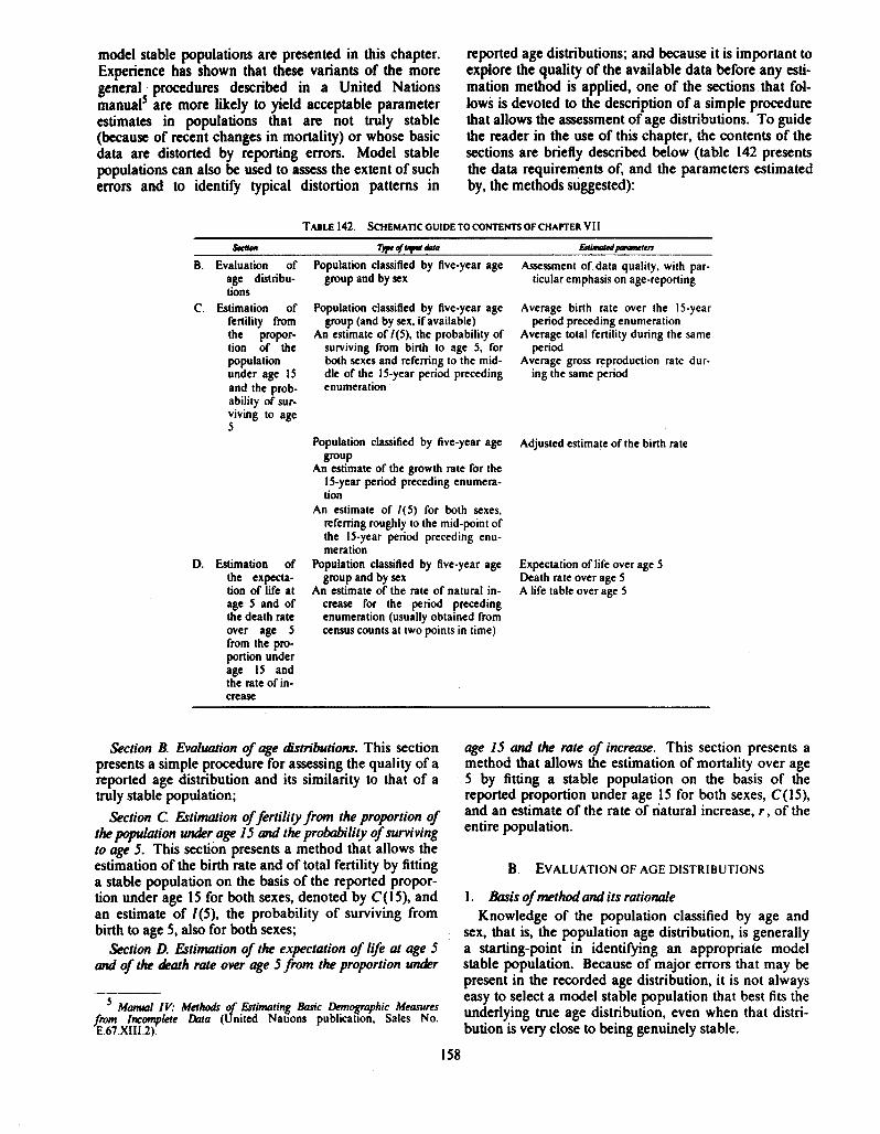
A simple procedure employing the Coale-Demeny model stable populations makes it possible to gain a visual impression of how closely the reported age distribution resembles a stable age distribution; or, con- versely, how much it is distorted by misreporting, selective omission or genuine differences. The method is based on a remarkable feature of stable populations that are within the same family (North, South, East or West) of the Coale-Demeny model stable populations. Each stable age distribution generated by a particular combination of a model life table and rate of increase is matched very closely by other stable distributions formed by life tables with the same overall pattern but with quite different levels of mortality, combined with different rates of increase. For example, as shown in figure 17, the following model stable populations in the family of West model stable populations for females are very similar: that with an expectation of life at birth of 35 years and a growth rate of 0.010; that with an expectation of life at birth of 45 years and a growth rate of 0.015; and that with an expectation of life at birth of 60 years and a growth rate of 0.020. In other words, a genuinely stable population can be rather closely matched (in terms of its proportions in successive five- year age groups, and especially in terms of its cumula- tive proportions under successive ages five years apart) by an appropriately chosen model stable population at an arbitrary level of mortality. It follows that, in erder to judge the congruence of a reported age distribution with that of a stable population, it suffices to compare the recorded age distribution with the model stable populations generated by a particular mortality level (arbitrarily chosen) and different rates of increase.

Specifically, the procedure recommended is the deter- mination of the sequence of birth rates. h ( x ). for x = 5.

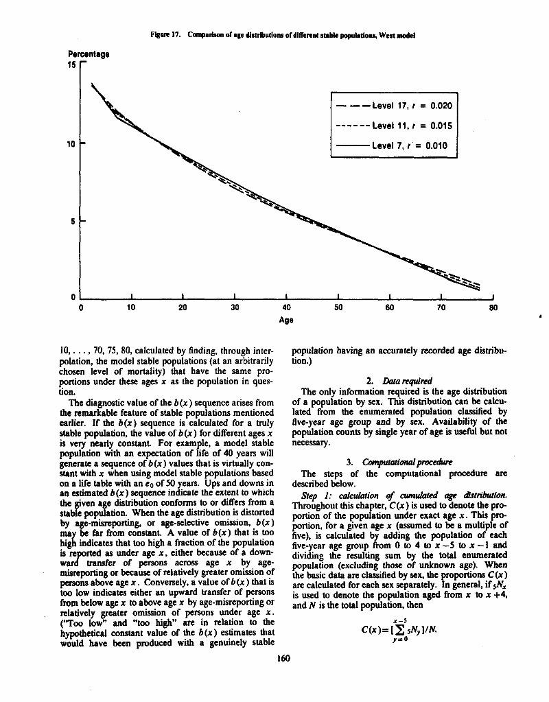
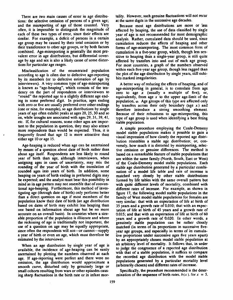
Figwe 17. Comparison of age distributions of different stable populations, West model

I___/ Level 17, r = 0.020

I --- - -- Level 11, r = 0.015 1 I Level 7, r = 0.010

10, . . . , 70, 75,80, calculated by finding, through inter- population having an accurately recorded age distribu- polation, the model stable populations (at an arbitrarily tion.) chosen level of mortality) that have the same proportions under these ages x as the population in ques- 2. &tareqwqwred tion. The only information required is the age distribution

The diagnostic value of the b(x) sequence arises from of a population by sex. This distribution can be calcu- the remarkable feature of stable populations mentioned lated from the enumerated population classified by earlier. If the b(x) sequence is calculated for a truly five-year age group and by sex. Availability of the stable population, the value of b(x) for different ages x population counts by single year of age is useful but not is very nearly constant. For example, a model stable necessary. population with an expectation of life of 40 years will generate a sequence of b(x) values that is virtually con- 3. Gmputational procedure stant with x when using model stable populations based The steps of the computational procedure are on a life table with an eo of 50 years. Ups and downs in described below. an estimated b(x) sequence indicate the extent to whlch aep 1: C ~ ~ o t i o n of dlribhtion. the given to Or differs from a Throughout this chapter, C(x) is used a denote the pm- stable population. When the age distribution is distorted podon of the population under exact age hi^ pro- by age-mkwpohng, or age-selective omission, b(x) portion, for a given age x (assumed to be a multiple of may be far from constant- A b(x) that is five), is calculated by adding the population of each high indicates that too high a fraction of the population five-year age group from 0 to 4 to -5 to - 1 and is as under age x* either because of a dividing the resulting sum by the total enumerated ward of pemm across age by age- population (excluding those of unknown age). When mhwpohng or because of greater the basic data are classified by sex, the propadons C(x) vns above age x. a b(x ) that is are calculated for each sex separately. In general, if 5NX too low indicates either an upward transfer of persons is =d to denote the population aged from to +4, from below age x to above age x by age-misreporting or is the total population, then relatively greater omission of persons under age x. ('Too low" and "too high" are in relation to the x -5

hypothetical constant value of the b(x) estimates that c ( x ) = [ C 5Ny11N would have been produced with a genuinely stable y = 0

160

Percentage 15

10

5

0 ,

'

-

-

i I I I I I I I 0 10 20 30 40 50 60 70 80

Age

Step 2: estimation of a set of mpmsentatiw birth rates at mortality level 13 4 the We-Demeny model stable populations. This step constitutes the computational core of this procedure; and it requires that, within the set of model stable populations subject to mortality level 13 of the Coale-Demeny life-table system, those whose proportions under ages x match the reported C(x) values be identified by means of a birth rate. To indicate that a given birth-rate estimate determines the stable population consistent with the observed C(x) value at mortality level 13, such an estimate is denoted by b(x). Note should be taken that this birth rate still refers to the whole of the stable population. The index x does not mean that only a portion of the stable population is considered.

The set of b(x) estimates is obtained by interpolating linearly (see annex IV) between the printed C(x) values of €he model stable populations. For a given, reported value of C(x), denoted by Co (x), the two stable populations whose C(x) values bracket this value (in the sense that C I(X) <Co .(x ) <C2(x )) are identified; and b (x ) is obtained by interpolating between their corresponding birth rates, denoted here by bl(x) and b z ( x ) , respectively. The detailed example that follows will help to clarify this calculation process.

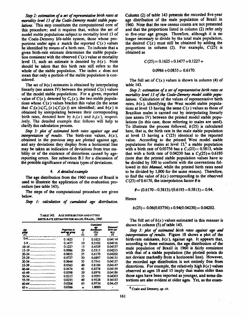
st& 3: plot 4 esti&ted birth rates against age and inte'pretation of msults. The birth-rate values, b (x ), obtained in the previous step are plotted against age, and any deviations they display from a horizontal line may be taken as indication of deviations from true stability or of the existence of distortions caused by age- reporting errors. See subsection B.l for a discussion of the possible significance of certain types of deviations.

4. A detailed example The age distribution from the 1960 census of Brazil is

used to illustrate the application of the evaluation procedure (see table 143).

The steps of the computational procedure are given below.

Step 1: calculation of cumulated age dstribution.

TABLE 143. AGE DISTRIBUTION AND FITTED BIRTH-RATE ESTIMATES FOR MALES. B WIL. 1960

Column (2) of table 143 presents the recorded five-year age distribution of the male population of Brazil in 1960. Note that the raw census counts are not presented and that the proportions listed in column (2) refer only to five-year age groups. Therefore, although it is no longer necessary to divide by the total male population, the desired C(x) must still be obtained by adding the proportions in column (2). For example, C(25) is obtained as

The full set of C(x) values is shown in column (4) of table 143.

Step 2: estimation of a set of mpresentatiw birth rates at mortality level 13 of the We-Demeny model stable populations. Calculation of the values of representative birth rates, b(x), identifying the West model stabie populations at level 13 having the same C(x) values as those of Brazilian males is carried out by interpolating linearly (see annex IV) between the printed model stable populations (in this case, those refemng to males are used). To illustrate the process followed, b(25) is calculated here, that is, the birth rate in the male stable population at level 13 having a C(25) identical to the reported value. According to the printed West model stable populations for males at level 13: a stable population with a birth rate of 0.03756 has a C1(25)= 0.5813, while that with a birth rate of 0.04230 has a C2(25)= 0.6193 (note that the printed stable population values have to be divided by 100 to conform with the conventions followed in this Manual, while the printed birth rates need to be divided by 1,000 for the same reason). Therefore, to find the value of b(x) corresponding to the'observed C(25) of 0.6 170, the interpolation factor B is

Hence

The full set of b (x ) values estimated in this manner is shown in column (5) of table 143.

Step 3: plot of estimated birth rates agaircst age Md interpreation of .results. Figure 18 shows a plot of the birth-rate estimates, b(x), against age. It appears that, according to these estimates, the age distribution of the male population of Brazil in 1960 is fairly consistent with that of a stable population (the plotted points do not deviate markedly from a horizontal line). However, the recorded age distribution is not entirely free from distortions. For example, the relatively high b(x) values observed at ages 10 and 15 imply that males older than t h ~ ages have been reported as younger, and some distortions are also evident at older ages. Yet, as the exam-

Age x

ples that appear in the next section prove, the observed distortions are minimal; and, in and by themselves, they would not be sufficient to preclude the use of estimation methods based on model stable populations in this case.

5. l)pidpdknu o / t k birth-- uli?naw

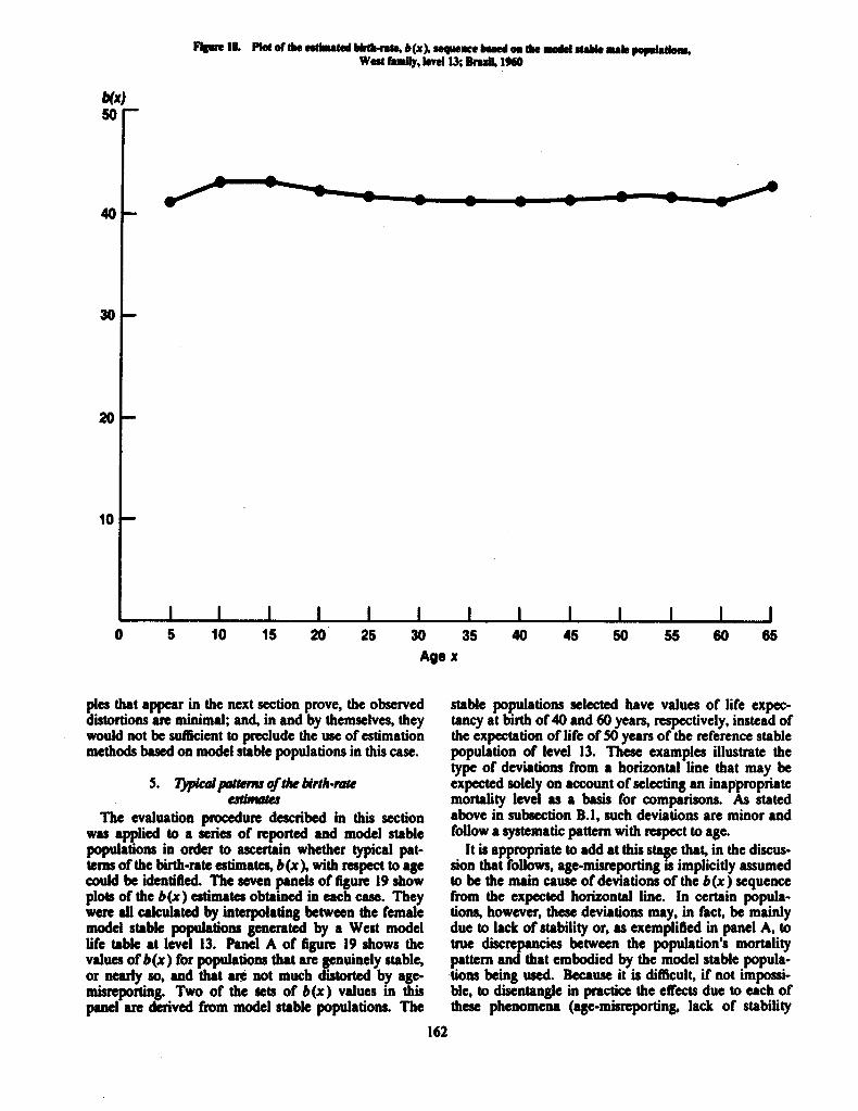
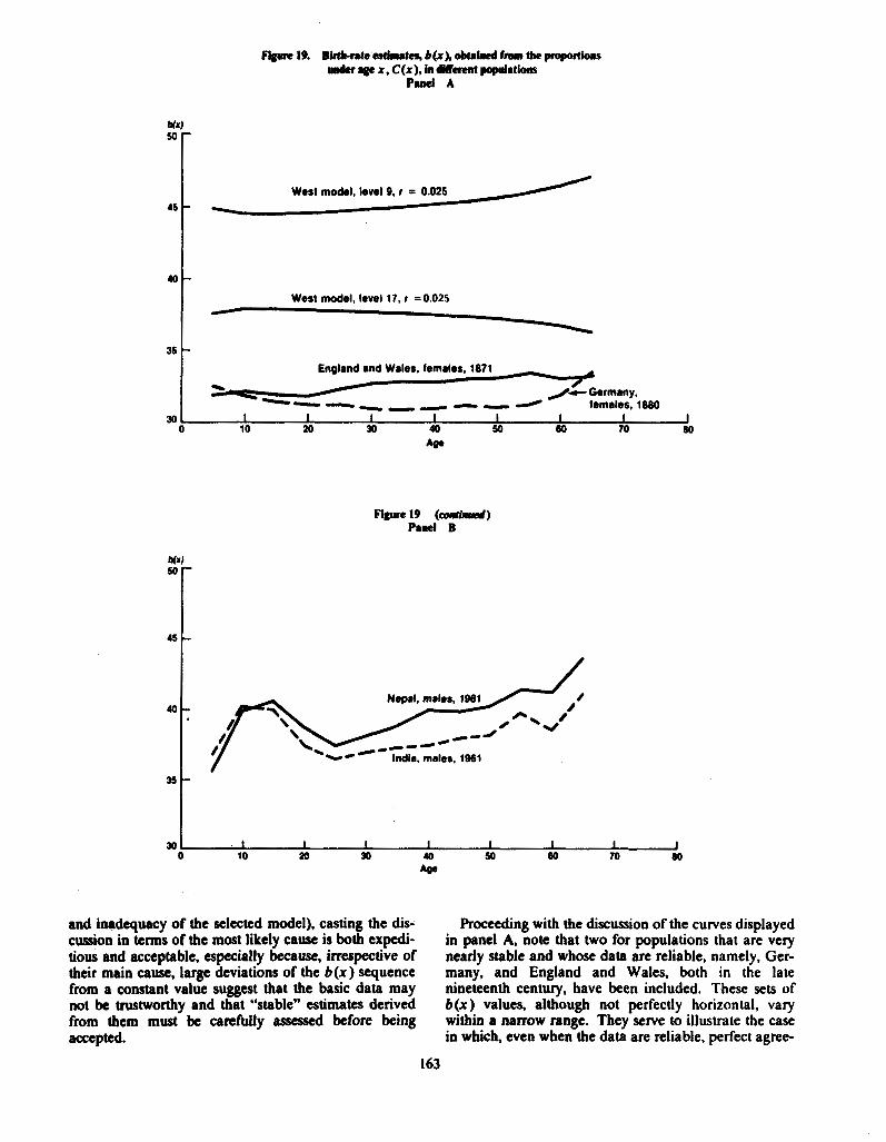
The evaluation procedure described in this section was applied to a series of reported and model stable populations in order to ascertain whether typical patterns of the birth-rate estimates, b (x ), with respect to age could be identified. The seven p e l s of figure 19 show plots of the b(x) estimates obtuned in each case. They were dl calculated by interpolating between the female model stable populations generated by a West model life 1.Mt at level 13. Panel A of Agure 19 shows the values of b(x) for populations that are genuinely stable, or nearly so, and that are not much distorted by age- misnporting. Two of the a ts of b(x) values in this panel are derived from model stable populations. The

stable populations selected have values of life expectancy at birth of 40 and 60 years, respectively, instead of the expectation of life of 50 years of the reference stable population of level 13. These examples illustrate the type of deviations from a horizontal line that may be expected solely on account of selecting an inappropriate mortality level as a basis for comparisons. As stated above in subsection B.l, such deviations are minor and follow a systematic pattern with respect to age.

It is appropriate to add at this stage that, in the discussion that follows, age-misrcporting is implicitly assumed to be the main cause of deviations of the b(x) sequence from the expected horizontal line. In certain populations, however, these deviations may, in fact, be mainly due to lack of stability or, as exemplified in panel A, to true discrepancies between the population's mortality pattern and that embodied by the model stable popula- .tions being used. Because it is difficult, if not impossible, to disentangle in practice the effects due to each of these phenomena (age-misnporting, lack of stability

19. BWuatc atimtes, b(x), obtahed fmm tbe proportions un&r age x . C(x), in Merent populations

P d A

-1 - West model, level 9, r = 0.025

West model, level 17. r = 0.025

5

Figure 19 (continual) Pane1 B

0

India. males, 1961

and inadequacy of the selected model), casting the discussion in tenns of the most likely cause is both expedi- tious and acceptable, especially because, irrespective of their main cause, large deviations of the b(x) sequence from a constant value suggest that the basic data may not be trustworthy and that "stable" estimates derived from them must be carefully assessed before being accepted.

Roceeding with the discussion of the curves displayed in panel A, note that two for populations that are very nearly stable and whose data are reliable, namely, Ger- many, and England and Wales, both in the late nineteenth century, have been included. These sets of b(x) values, although not perfectly horizontal, vary within a narrow range. They serve to illustrate the case in which, even when the data are reliable. perfect agree-

' \ India, females, 1961

I Nepal, f G l e s , 1961

- - - aham, mahr, 1960 - Morocco, males, 1960

ment between the models and the observed data is not achieved.

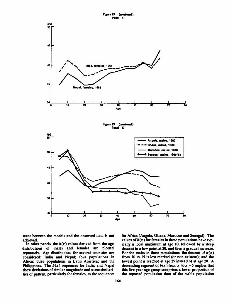
In other panels, the b(x) values derived from the age distributions of males and females are plotted separately. Age distributions for several countries are considered: India and Nepal; four populations in Africa; three populations in Latin America; and the Philippines. The b(x) sequences for India and Nepal show deviations of similar magnitude and some similari- ties of pattern, particularly for females, to the sequences

for Africa (Angola, Ghana, Morocco and Senegal). The values of b(x ) for females in these populations have typ ically a local maximum at age 10, followed by a steep descent to a low point at 20, and then a gradual increase. For the males in these populations, the descent of b(x) from 10 to 15 is less marked (or non-existent); and the lowest point is reached at age 25 instead of at age 20. A descending segment of b(x) from x to x +5 implies that this five-year age group comprises a lower proportion of the reported population than of the stable population

- - - ahma, kmales, 1960 - Morocco, iemabs, 1960

- Brazil, males, 1960 - -- Mexico, msles. 1960 - Peru, males, 1961 - Philippines, males, 1960 I fitted to C(x), and a rising segment implies that there is a higher proportion of the reported population in this five-year age internal than in the stable population with the same C(x ). Thus, the rise in the b(x ) sequences for India and Nepal from age 5 to age 10 implies a reported proportion in age group 5-9 higher than that in the stable population, and the universal decline from 10 to 15 and from 15 to 20 for females implies that these two age groups (10-14 and 15-19) comprise a lower proportion of the reported than of the stable population. The low values at 20 and 25 imply a substantial upward

transfer (caused by age-misreporting) across these two age boundaries.

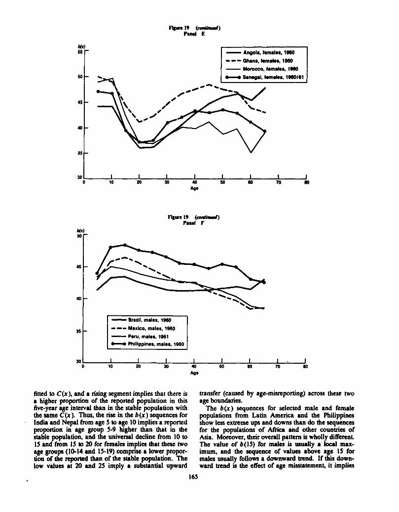
The b(x) sequences for selected male and female populations from Latin America and the Philippines show less extreme ups and downs than do the sequences for the populations of Africa and other countries of Asia. Moreover, their overall pattern is wholly different. The value of b(l5) for males is usually a local mu- imum, and the sequence of values above a e 15' for mala usually follows a downward mnd. If $ downward trend is the effect of age misstatement, it implies

-- -- - Mexico, females, 1960 - Peru, females, 1961

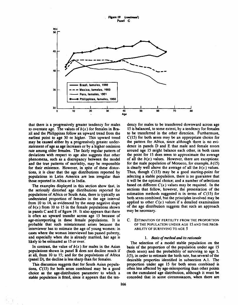
that there is a progressively greater tendency for males to overstate age. The values of b(x) for females in Bra- zil and the Philippines follow an upward trend from the earliest point to age 50 or higher. This upward trend may be caused either by a progressively greater under- statement of age as age increases or by a higher omission rate among older females. The fairly regular pattern of deviations with respect to age also suggests that other phenomena, such as a discrepancy between the model and the true patterns of mortality, may be responsible for their existence. However, in spite of these distortions, it is clear that the age distributions reported by populations in Latin America are less irregular than those reported in Africa or in India.

The examples displayed in this section show that, in the seriously distorted age distributions reported for populations of Africa or South Asia, there is typically an understated proportion of females in the age interval from 10 to 14, as evidenced by the steep negative slope of b(x) from 10 to 15 in the female populations shown in panels C and E of figure 19. It also appears that there is often an upward transfer across age 15 because of age-misreporting in these female populations. It is probable that such misstatement arises because the interviewer has to estimate the age of young women: in cases where the woman interviewed has passed puberty, and especially when she is already married, her age is likely to be estimated as 15 or over.

In contrast, the value of b(x) for males in the Asian populations shown in panel B does not decline much if at all, from 10 to 15; and for the populations of Africa (panel D), the decline is less sharp than for females.

This discussion suggests that for South Asian populations, C(15) for both sexes combined may be a good choice as the age-distribution parameter to which a stable population is fitted, since it appears that the ten-

dency for males to be transferred downward across age 15 is balanced, to some extent, by a tendency for females to be transferred in the other direction. Furthermore, C(15) for both sexes may be an appropriate choice for the pattern for Africa, since although there is no evidence in panels D and E that male and female errors around age 15 might balance each other, in both cases the point for 15 does seem to approximate the average of all the b(x ) values. However, there are exceptions: for the male population of Morocco, for example, b(15) is clearly well above the average of all the b (x) values. Thus, though C(15) may be a good starting-point for selecting a stable population, there is no guarantee that it will be the optimal choice; and a number of selections based on different C(x) values may be required. In the sections that follow, however, the presentation of the estimation methods suggested is in terms of C(15) for both sexes combined, but the principles involved may be applied to other C(x ) values if a detailed examination of the age distribution suggests that such an approach may be necessary.

C. ESTIMATION OF FERTILITY FROM THE PROPORTION OF THE POPULATION UNDER AGE 15 AND THE PROB- ABILITY OF SURVIVING TO AGE 5

1. h i s of method and its rationale The selection of a model stable population on the

basis of the proportion of the population under age 15 (both sexes) and the probability of surviving to age 5, 1 (5), in order to estimate the birth rate, has several of the desirable properties identified in subsection A.1. The proportion under age 15 for both sexes combined is often less affected by age-misreporting than other points on the cumulated age distribution, although it must be conceded that in some circumstances, when there are

high omission rates of young children or when certain problems arise at the time of interview (as, for instance, when heaping concentrates at age 14 as a result of women trying to avoid being interviewed individually in surveys where the target population is that aged from I5 to 49), C(15) can be either too low or too high. There- fore, although fairly robust to the effects of typical age- misreporting patterns, the estimation methods based on C(15) may still yield biased estimates in particular situa- tions. Hence, a careful evaluation of the accuracy of C(15) is recommended before these methods are applied.

The use of l(5) as an indicator of mortality in childhood also enhances the overall robustness of this method. As described in chapter 111, l(5) can be estimated from the proportion of children surviving among those ever borne by women aged from 30 to 34 (or duration of marriage of 10-14 years). This estimate of mortality is usually fairly reliable; and when mortality has been changing, it refers to a period located some six or seven years before the time of the interview, about the appropriate time reference for estimating the average birth rate during the 15 years preceding enumeration.

Thirdly, model stable populations identified on the basis of values of C(1S) and l(5) from the four families of Coale-Demeny models have nearly the same birth rate and the same total fertility. Such consistency does not extend to stable populations from the different' models having the same C(15) and rate of increase. For example, in model stable populations with a C(15) value of 0.4195 and an l(5) of 0.8185, the birth rate ranges only from 0.0408 to 0.0414; and total fertility varies only from 5.70 to 5.89 (to calculate these total fertility rates, the mean age of the fertility schedule was assumed to be 29 years and the sex ratio at birth used was 105 male births per 100 female births). On the other hand, in model stable populations with the same value of C(15) (0.4195) and a rate of increase of 0.025, the birth rate ranges from 0.0408 to 0.0440 and total fertility varies from 5.70 to 6.22.

Lastly, and most surprisingly, the selection of a model stable population on the basis of C(15) and l(5) provides an estimate of the birth rate that closely matches the average birth rate during the 15 years preceding enumeration, even when the population in question is far from stable.

The remarkable accuracy of this approximation in the case of non-stable populations can be explained in heuristic terms by viewing the estimation of a stable birth rate from C(15) and l(5) as a form of reverse projection yielding an estimate of the average birth rate during the 15 years preceding the time of enumeration. In a stable population, the average birth rate during this period is, of course, the same as the current birth rate, but it could be estimated from the stable age distribution by the conventional procedure of reverse projection. The number of births in the period, estimated by reverse projection to birth &f the population in each age interval under 15, divided by the number of person-years lived

during the period by the total population (estimated by reverse projection of the current population using the stable rate of natural increase), would yield the desired birth-rate estimate. For a non-stable population, the equivalent calculations would involve the same reverse projection to birth of the persons in each five-year age group in the 0-14 range, and the division of the resulting total number of births by the total population reverse- projected according to the actual rate.of increase.

A stable population selected so that its parameters match the observed C(15) and l(5) values must incor- porate a life table with l(x) values up to age 15 that are fairly similar to those characterizing mortality in the given population over the preceding 15 years or so. The repofled population under 15 may be allocated to the three five-year age groups in the 0-14 range in a different way than that of the fitted stable population, but because of the low mortality rates that usually characterize these ages (at least from age 3 to age 14), the differences in the age distribution under 15 between the reported and the stable populations should have only a slight effect on the number of births calculated by reverse projection. Thus, the fitted stable population may be expected to provide an adequate representation of the numerator of the birth rate, that is, the number of births in the preceding 15 years.

A more important difference is likely to affect the denominator; and it arises from differences between the observed and the stable rates of increase, especially if there has been a recent change in fertility. In such an instance, the stable population fitted to the observed C(I5) and l(5) values is unlikely to have the same growth rate as the reported population had over the preceding 15 years; in general, the stable population has a lower growth rate. Continuing with the analogy to reverse projection, the birth rate of the stable population could be improved, as an estimate of the true average birth rate over the preceding 15 years, if an adjustment were made for the difference between the true and the stable growth rates in order to estimate more accurately the denominator of the birth rate. If the stable growth rate is lower than the true growth rate, according to the reverse-projection analogy, it would result in somewhat too high an estimate of the person-years lived by the population over the preceding 15 years, which in turn would give rise to too low an estimate of the birth rate. Thus, the birth rate can be adjusted upward by multiplying it by the ratio of the number of person-years lived implied by the stable growth rate to the true number of person-years actually lived by the reported population, that is, by No exp [ -7.5r,]/N0 exp [ -7.5r0], where No is the total reported population; r, is the stable growth rate; and ro is the reported growth rate. If the difference between the true average growth rate over the preceding 15 years and the growth rate of the fitted stable population is 0.002 (say, a true value of 0.022 against a stable value of 0.020). for instance, the adjustment for the denominator can be made directly to the birth rate of the fitted stable population, multiplying it by the factor exp [7.5(0.022-0.020)]. The adjustment would thus be about 1.5 per cent upward. A similar procedure should

also prove effective in cases of destabilization resulting from mortality change. It should be pointed out, however, that the adjustment does not always improve the initial estimate of the birth rate, particularly in the case of very recent fertility change. Further, the adjustment may not be suitable in practice if the reported growth rate is distorted by changes in enumeration completeness.

Table 141 shows the results obtained when this estimation procedure was applied to several populations with accurate birth registration. The average birth rates estimated from l(5) and C(15) are compared with the average birth rates registered during the 15-year period preceding each census. In the first part of table 141,1(5) has been estimated from data on children ever born and surviving. In the second part, covering countries for which such data are not available, the value of l(5) has been taken from official life tables referring approximately to the period 7.5 years before each census. In these cases at least, the procedure yields very good estimates of the birth rate for populations that are clearly not stable.

2. &a ~qau'red The following data are required for this method: (a) The enumerated population classified by five-year

age group and by sex. Strictly speaking, only the population of both sexes under age 15 and the total population enumerated are required. However, in order to assess the quality of the data (for example, by using the procedure described in section B), further classification by sex is necessary;

(b) An estimate of l(5) for both sexes combined referring approximately to the period between six and eight years before the time of enumeration. (Refer to chapter I11 for methods yielding this estimate from data on children ever born and surviving.);

(c) An estimate of net migration during the period preceding the time at which the population was enumerated. If net migration is substantial, stable population analysis should be carried out only after the reported age distribution has been adjusted for its effects;

(d ) An estimate of the sex ratio at birth; (e) An estimate of the growth rate during the 15 years

or so preceding enumeration (this estimate is necessary only if there is evidence suggesting that the reported population is not approximately stable and if, as a result, an adjustment of the stable birth rate for the difference between the reported and stable growth rates is desirable).

3. Compuationalpnmchw Step 1: calculation of pportion under age 15 for both

sexes. The calculation of this proportion, C(lS), is carried out according to the general principles described in step 1 in subsection 8.3. Essentially,

to x +4; and N is the total enumerated population (excluding those of unknown age).

Step 2: i&ntijication of a mortality level consistent with thepmbability of surviving to age 5. The desired mortality level is identified by interpolating linearly (see annex IV) between the probabilities of surviving to age 5,1 (S), listed in annex VIII for the mortality pattern selected as most suited for the country concerned. Note that the mortality level should be found for males or females, but not for both sexes combined, since although I(5) refers to both sexes combined, identification of a mortality level is carried out using the tables referring to a given sex (male or female). The reason for this procedure is that model stable populations referring to both sexes combined are not published in the Coale-Demeny volume?

Step 3: idmtificution of the stable population with the same pbtahlity of surviving to age 5 and proportion under: age 15 as the nporled population. Using the mortality level identified in step 2 and the selected family of models for a given sex (male or female), two populations at the estimated mortality level are found whose proportions under age 15 enclose the reported C(15) for both sexes, denoted by Co(15), in the sense that C1(15), (C' (15)<C2(15). Once identified, interpolation between the parameter values of the two stable populations yields the required stable estimates (the birth rate, the growth rate and the death rate, for example). Note again that, although the observed Co (15) refers to both sexes combined, interpolation is carried out only within the stable populations referring to one selected sex (male or female). This procedure implies that one is assuming the underlying pattern of mortality of both sexes of the population under study to be similar to either the male or female model chosen as reference.

Step 4: calculation of p reproduction rate and of total fertility for the selected stable population. The population identified in step 3 refers to both sexes combined, so that the calculation of parameters that refer only to the female population is not straightforward. To obtain their values, it is necessary to identify the female stable population associated with that already selected for both sexes combined. A serviceable choice of a female stable population is made by estimating the female birth rate as

where b, is the estimated birth rate for both sexes combined; B /B, is the proportion of births that are female (B stan d for the number of births); and N /N, is the h proportion of the population that is female ( stands for number of persons). The proportion of female births can be taken as about 48.8 per cent of the total, except in tropical Africa, or in populations of primarily African origin, where a proportion of about 49.3 per cent should

C(15)= GNo+jNj +sNlo)/N (C.1)

when jN, is the population of both sexes aged from x ' IM.

be used. The proportion female in the population can be taken from the census, unless sex selective omission is evident.

Note that Bf /B, can also be written as

where SRB is the sex ratio at birth defined as the number of male births per female birth. Therefore, knowledge of SRB and of the total male and female population counts is sufficient to calculate bI from 6,.

Once bl is available, using the mortality level identified m step 2, the value of the gross reproduction rate, GRR, can be estimated by interpolation within the female set of stable populations of the family being used. However, the printed model stable populations give only estimates of the gross reproduction rate for certain mean ages of the fertility schedule. It is recommended that a first estimate of this rate be calculated by setting this mean age, p, to 29. Then if p can be more accurately estimated for the population in question (see annex 111). the preliminary GRR(29) estimate can be adjusted by using the following relation:

GRR (p) = GRR (29) exp((p - 29Xr +&))I (C.4)

where &) is the death rate at p and is estimated as

where 5M, is the central death rate for females aged from x to x +4 in the life .table at the level identified in step 2.

Lastly, an estimate of total fertility is obtained as

It should be mentioned that step 4 should not be carried out if there is evidence suggesting that the population being studied is not approximately stable, since the estimates obtained according to the procedures described in this step refer only to a stable population. Therefore, especially when fertility has been declining, these estimates may be misleading.

Step 5: @ushnent of stable birth-mte estimate when the population is not truly stable. If there is evidence suggesting that the population has experienced important fertility and mortality changes, the stable birth rate obtained in step 3 cannot be considered an adequate estimate of the corresponding parameter of the true population. Fortunately, if the average growth rate of the population during the 15 years or so preceding the time of enumeration is known, the stable birth rate estimate may be adjusted for the effects of declining fertility. As in other instances, the required growth rate is estimated on the basis of population counts at different points in time. The equation used to calculate it is

where 4 is the total population enumerated at time ti (including those of unknown age).

When r, is different from the stable growth rate, r, , estimated in step 3, the stable birth-rate estimate also obtained in that step can be adjusted by

4. A detailed example The case of Brazil in 1960 is used as an example. A

census with 1 September as reference date was camed out in that year. Its results have already been used in chapter 111, subsection E.4 (b) to obtain estimates of child mortality. Furthermore, the reliability of the reported age distribution of the male population was assessed above in subsections B.4 and B.5. As is often the case, the proportion under age 15 for males appears to be overstated, while there is no unambiguous bias in the female C(15) (see panels F and G of figure 19). Hence, there seems to be no reason for fitting a stable population to any C(x) in preference to C(15); but, bearing in mind that errors in the male and female C(15) values may not cancel each other out in this case, for illustrative purposes the method described in this section is applied.

The steps of the computational procedure are given below.

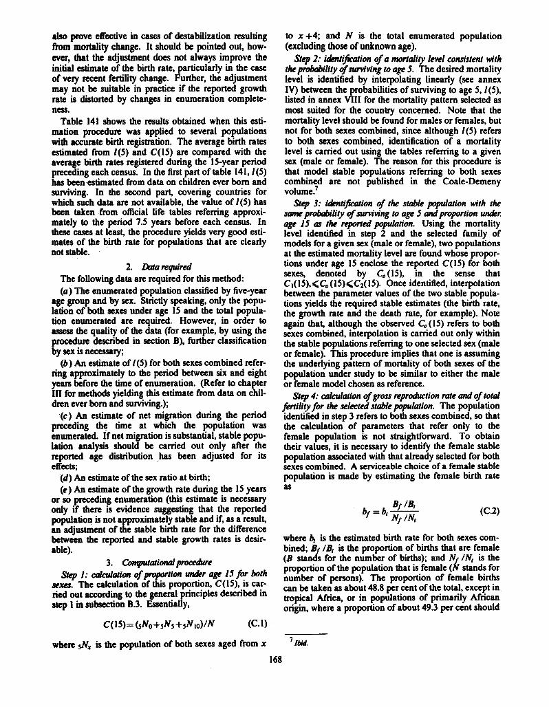
Step I: calculation of pmportion w&r age 15 for both sexes. Table 144 presents the basic population counts in the form of cumulated numbers of persons under selected ages. Classification by sex is available. Accord- ing to this table,

while

so that

TABLE 144. POWIATION UNDER EXACT AGE& N(x -) BY SEX. BIUZIL, I960 (-1

Step 2: identi$cation of a mortaliy level consistent with the ptoboblity of surviving to age 5. The estimation of child mortality from data on children ever born and surviving collected during the 1960 census of Brazil, was camed out in chapter 111, subsection E.4 (b). Table 79 in that chapter contains the raw data, while table 80 shows the resulting child mortality estimates. The estimate of l(5) for both sexes combined is 0.8222. In subsection E.4 (b) of chapter 111, it was stated that if the sex ratio at birth of the Brazilian population is assumed to be 1.05 male births per female birth, this value of l(5) is consistent with level 13.6 of the West model life tables for both sexes combined. However, if in the application of the methods described in this chapter one were to use consistently life tables for both sexes combined, it would be necessary to generate new stable populations using those Life tables, since the Coale and Demeny tables refer only to males or females separately. Given the robustness of the methods described here to variations in the model patterns of mortality (see section C.1), it does not seem necessary to insist on absolute consistency by using stable populations refemng to both sexes combined. It is more expedient and scarcely less satisfactory from the point of view of the accuracy of the estimates obtained to use the sex-specific model stable populations published in the Coale-Demeny set as if they were adequate representations of the experience of both sexes combined. This approach is equivalent to assuming that if, for example, only the female tables are used, the mortality pattern embodied in the female life tables is an adequate representation of the mortality pattern prev- alent in the whole population (both sexes combined). In the case of the method at hand, this assumption is more satisfactory than it would appear at first sight because only the mortality up to age 15 is of major importance; and for the age range 0-14, differences between the mortality pattern for both sexes combined and those for each one separately are relatively small.

In the case of Brazil in 1960, the female life tables for model West a n assumed to be adequate representations of true mortality pattern. Accordingly, the model l(5) values listed in table 236 (see annex VIII) are used to identify the mortality level corresponding to the observed value of 0.8222. As usual, linear interpolation is used (see annex IV) to find this level. The process involves searching the values listed under label "1 (5)" in table 236 for two values that enclose the observed l(5). In this case, they are ll3(15)= 0.81848 and 114(15)= 0.84106, where the subindices indicate the level

with which each value is associated. Then, the interpolation factor 8 is obtained as

Hence, the female West level desired is 13.16. Step 3: i&ntijication of the stable population with the

same probability of surviving to age 5 andproportion under age 15 as the mpwted population. The first task in this step is to calculate the values of the proportion under age 15, C(lS), at level 13.16 for West female stable populations with different birth rates (or growth rates). Refemng to the printed stable age distributions, one finds that at level 13, C1(15)= 0.4195 for a population with an annual growth rate of 0.025, and C2(15)= 0.4539 for a population growing annually at a qte of 0.030. The c?rresponding values at level 14 are C1(l 5) = 0.4 14 1 and C2(1 5)= 0.4487. Hence, in order to obtain the corresponding estimates at level 13.16, one uses the interpolation factor 8 of 0.16 as follows: .

where the superindex indicates that the C(15) values correspond to level 13.16. It remains to find the growth rate and birth rate with which the reported C(15)= 0.4268 is associated. Note that the C *(15) estimates presented above enclose the reported value as desired. The reported C(l5) is used to interpolate between the C*(15) values, the necessary interpolation factor being

The growth rate associated with the reported C(15) is found using 8:

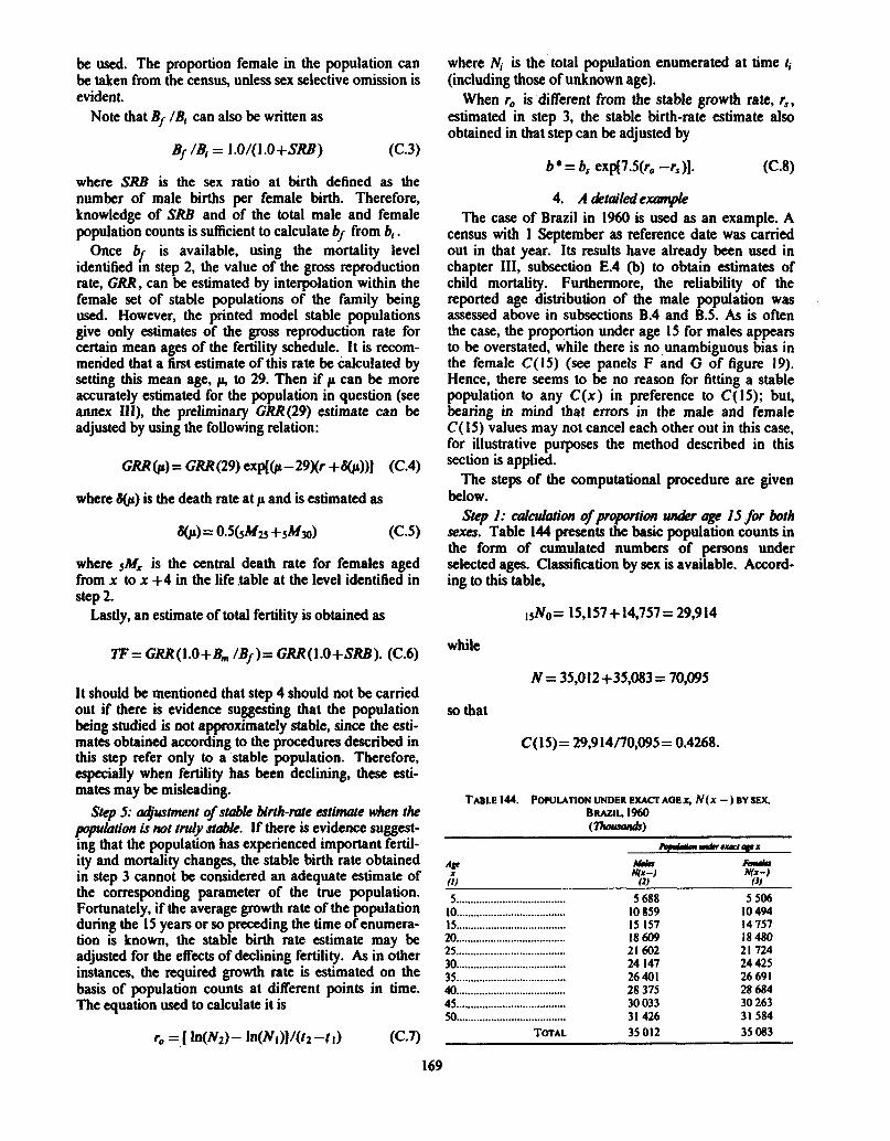
Table 145 shows some of the intermediate results of these calculations. It also gives the estimates of the birth rate. Those at level 13.16 for growth rates 0.025 and 0.030 are obtained exactly in the same way as the C*(15) estimates given above. The birth rate for r, = 0.0262 is then calculated as

TABLE 145. IDENTIFICATION OF THE STABLE POPULATION DETERMINED BY THE REPORTED PROPORTION UNDER AGE 15 AT LEVEL 13.16, BIIAZIL. 1960

This value is therefore the stable estimate of the birth rate.

Stcp 4: cakulation of grau npraduction rate and of total fertility for the selected stablc ptpdation. As is shown in the next section, the stable population identified in step 3 is not an adequate representation of the Brazilian population in 1960. Hence, it makes no sense to calculate at this point other parameters of this stable population, because they are not likely to be acceptable as estimates for the'actual population. For this reason, the application of step 4 is deferred (see subsection C.5).

Step 5: @wbnent of stable birth-me estimate Wiren the ppdation is not t d y stable. Brazil carried out censuses on 1 July 1950 as well as on 1 September of 1960, and they yielded total population counts (including persons of unknown age) amounting to 51,916,000 and 70,119,000 persons, respectively. Hence, the 1950- 1960 intercensal growth rate is calculated as follows:

This growth rate is evidently much higher than that estimated in step 3 for the fitted stable population. Such a discrepancy suggests either that the Brazilian population was not stable, as a result of mortality or fertility changes the influence of which on the estimated birth rate must be taken into account, or that some other methodological problems may exist. Ignoring for the moment the possibility of the latter situation, for the sake of illustration, an adjusted birth rate is calculated by using equation (C.8) as follows:

5. c4mwmrs on the &tartarilcd exmple Several remarks must be made about the example just

presented and, as will be seen, some will lead to the complete modification of the estimates found above. The first comment, however, is mostly of a methodological nature and refers to the question whether male or female model stable populations should be used in applying this method. In the case just analysed, if the male West model stable populations had been used, the observed l(5) for both sexes combined would have implied a mortality level of 13.97, and the preliminary estimates of the stable birth rate and growth rates would have been 0.04155 and 0.0260, respectively. Adjustment of the former by exp(7.5(0.0035)] = 1.0265 would have yielded a final birth rate estimate of 0.04265, in which the first three significant figures agree with those of the estimate obtained in step 5 by using the female models. This is yet another example of the robustness of the estimation procedure to changes in the model mortality pattern d.

Next to be considered is an evaluation of the estimates obtained. The difference between the estimated stable

growth rate of 0.0262 and the intercensal growth rate of 0.0295 could arise either because the 1960 ansus was more complete than the 1950 ansus, or because the West mortality pattern is an inadequate representation of the mortality of the Brazilian population (higher growth rates would be expected in populations with a given C(15) subject to heavier mortality below age 5 and lower mortality above age 5 than those embodied by the West model).

To assess the influence that the selection of a certain mortality model has on the final estimates and to explore the fits of other models, the estimation process is repeated using the South model. The first step is to obtain adequate child mortality estimates also referring to the South model. The appropriate coefficients given in table 47 (see chapter 111) and the observed P(l)/P(2) and P(2)/P(3) ratios given in table 80 (see chapter III), together with D(4), are used to obtain the required estimate of l(5). Its value for both sexes is 0.8201, implying a mortality level of 14.85 in the female tables. Repeat- ing step 3 with the South family, the preliminary estimate of the birth rate obtained from C(15) at level 14.85 is 0.0423 1, and the corresponding estimate of the growth rate is 0.02859. Had male stable populations been used instead of female, the corresponding results would have been 0.04221 and 0.02805, showing that the choice between the sex-specific stable models is not important. This growth rate is comfortingly close to the intercensal growth rate, implying an adjustment factor of only 1.0068 for the stable birth rate, the adjusted birth rate estimate being therefore 0.04260. The fact that this adjusted estimate virtually coincides with that obtained earlier using a different mortality model illustrates again the robustness to choice of mortality pattern of the method that uses 1(5), C(15) and r to estimate the birth rate. A very accurate estimate of the birth rate is possible (assuming, of course, that the underlying data are correct), regardless of whether the population is stable and without regard to the family of model stable populations employed in the calculation. In addition, the high level of agreement between the intercensal rate of increase and the estimated stable growth rate when the South family of stable populations is used supports the suitability of this model as a good representation of mortality patterns in Brazil during the 15-year period preceding 196G, provided, of course, that the intercensal estimate of the growth rate may be considered reliable.

Having established a best estimate of the birth rate for the Brazilian population during the 15 years or so preceding 1960, the rest of this section is devoted to the estimation of other parameters of the population being studied from those of the fitted stable population. For this purpose, step 4 of the detailed example is again presented below. Step 4: caldation of grars np&tion rate and of total

fertility for the sekted s t d e ptpdation. To estimate total fertility and the gross reproduction rate, it is necessary to identify a female stable population consistent with the observed population. This identification is based on the estimated l(5) for both sexes combined, the female birth rate implied by the final birth rate estimate

(6 = 0.0426). the sex ratio at birth and the sex ratio of che reported population. If one assumes that the sex ratio at b i d .is 1.05 male births per female birth, 48.8 per cent of all births are female, and since the fraction of the reported population that is female is

the birth rate for females is

bf = (0.0426X0.488)/0.5005 = 0.04 15.

Similarly, that for males is

& = (0.0426X 1 .O -0.488)/(1 .O -0.j005)

= (0.0426X0.5 12)/0.4995 = 0.0437.

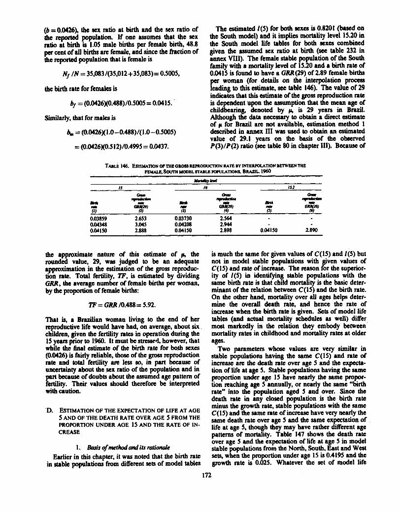
The estimated l(5) for both sexes is 0.8201 (based on the South model) and it implies mortality level 15.20 in the South model life tables for both sexes combined given the assumed sex ratio at birth (see table 232 in annex VIII). The female stable population of the South family with a mortality level of 15.20 and a birth rate of 0.0415 is found to have a GRR (29) of 2.89 female births per woman (for details on the interpolation proms leading b this estimate, see table 146). The value of 29 indicates that this estimate of the gross reproduction rate is dependent upon the assumption that the mean age of childbearing, denoted by is 29 years in Brazil. Although the data necessary to obtain a direct estimate of p for Brazil an not available, estimation method 1 described in annex I11 was used to obtain an estimated value of 29.1 years on the basis of the observed P(3)/P(2) ratio (see table 80 in chapter 111). Because of

TABh 146. ES~~MTION oP THE 0 ~ 0 ~ s ~ P R o D u ~ O N Mil! BY lNTEllPOUTlON BETWEEN THE ~ e r u ~ e . S o v m MODEL srrsste POWLATIONS. BRAZIL. 1960

the approximate naturc of this estimate of p, the rounded value, 29, was judged to be an adequate approximation in the estimation of the gross rcproduc- tion rate. Total fertility, TF, is estimated by dividing GRR, the average number of female births per woman, by the proportion of female births:

TF = GRR /0.488 = 5.92.

That is, a Brazilian woman living to the end of her reproductive life would have had, on average, about six children, given the fertility rates in operation during the 15 years prior to 1960. It must be stressed, however, that while t4e final estimate of the birth rate for bo.th sexes (0.0426) is fairly reliable, those of the gross reproduction rate and total fertility are less so, in part because of uacertainty about the sex ratio of the population and in part because of doubts about the assumed age pattern of fertility. Their values should therefore be interpreted with caution.

'D. ESTIMATION OF THE EXPECTATION OF LIFE AT AGE 5 AND OF THE DEATH RATE OVER AGE 5 FROM THE PROPORTION UNDER AGE 15 AND THE RATE OF IN- CREASE

1. h i s of methd and its rationale Earlier in this chapter, it was noted that the birth rate

in stable populations from different sets of model tables

is much the same for given values of C(15) and I(5) but not in model stable populations with given values of C(15) and rate of increase. The reason for the superior- ity of l(5) in identifying stable populations with the same birth rate is that child mortality is the basic deter- minant of the relation between C(15) and the birth rate. On the other hand, mortality over all ages help deter- mine the overall death rate, and hence the rate of increase when the birth rate is given. Sets of model life tables (and actual mortality schedules as well) differ most markedly in the relation they embody between mortality rates in childhood and mortality rates at older ages.

Two parameters whose values are very similar in stable populations having the same C(15) and rate of increase are the death rate over age 5 and the expectation of life at age 5. Stable populations having the same proportion under age 15 have nearly the same proportion reaching age 5 annually, or nearly the same "birth rate" into the population aged 5 and over. Since the death rate in any closed population is the birth rate minus the growth rate, stable populations with the same C(15) and the same rate of increase have very nearly the same death rate over age 5 and the same expectation of life at age 5, though they may have rather different age patterns of mortality. Table 147 shows the death rate over age 5 and the expectation of life at age 5 in model stable populations from the North, South, East and West sets, when the proportion under age 15 is 0.4195 and the growth rate is 0.025. Whatever the set of model life

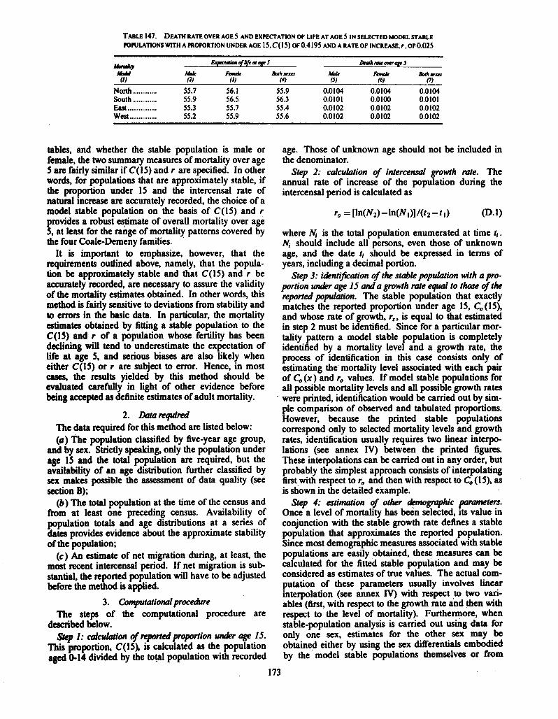
TABLE 147. DEATH RATE OVER AGES AND EXPECTATION OF LIFE AT AGE 5 IN SELECTED MODEL STABLE W U T I O N S WITH A PROPORTION UNDER AGE 15. C(15) OF 0.4 195 AND A RATE OF INCREASE. r . OF 0.025

Mnrmm E q e c t a t h ~ & m c y J I k a h r a t e m r ~ J

lb~l' Faplr Ibrh xur Mole Fen& Ibrh xur 111 111 (3) (4) f.0 (6) (7)

North ............. 55.7 56.1 55.9 0.0 104 0.0104 0.0104 South ............. 55.9 56.5 56.3 0.0101 0.0100 0.0101 East ................ 55.3 55.7 55.4 0.0102 0.0102 0.0102 Wcst ............... 55.2 55.9 55.6 0.0 102 0.0 102 0.0102

tables, and whether the stable population is male or age. Those of unknown age should not be included in female, the two summary measures of mortality over age the denominator. 5 are fairly similar if C(15) and r are specified. In other Step 2: cdCUlation of interned growth W e . The words, for populations that are approximately stable, if annual rate of increase of the population during the the proportion under 15 and the intercensal rate of intercensal period is calculated as natural increase are accurately recorded, the choice of a model stable population on the basis of C(15) and r = [ln(Nz)-ln(N~)l/(tz -t I) provides a robust estimate of overall mortality over age

(D.1)

5, at least for the range of mortality patterns covered by where 4 is the total population enumerated at time t,. the four Code-Demeny families. N, should include all persons, even those of unknown

It is important to emphasize, however, that the age, and the date t, should be expressed in terms of requirements outlined above, namely, that the popula- years, including a decimal portion. tion be approximately stable and that C(15) and r be Step 3: i&ntification ofthe stable population wfth a pro- accurately recorded, are necessary to assure the validity portion un&r age I5 and a growth mte equal to those ofthe of the mortality estimates obtained. In other words, this reported populaion. The stable population that exactly method is fairly sensitive to deviations from stability and matches the proportion under age 15, c0 (15), to emon in the basic data- In particular, the mortality and whose rate of growth, r,, is equal to that estimated estimates obtained by fitting a stable population to the in step 2 must be identified. Since for a particular mor- C(15) and r of a population whose fertility has been tality pattern a model stable population is completely declining will tend to underestimate the expectation of identified by a mortality level and a growth rate, the life at age 5, and serious biases are also likely when process of identification in this case consists only of either C(15) or r are subject to error. Hence, in most estimating the mortality level associated with each pair cases, the results Yielded by this method should be of Co ( x ) and ro values. If model stable populations for evaluated carefully in light of other evidence before all possible mortality levels and all possible growth rates being accepted as definite estimates of adult mortality. - were printed, identification would be cam'ed out by sim-

ple comparison of observed and tabulated proportions. 2. Doro required However, because the printed stable populations

The data required for this method are listed below: correspond only to selected mortality levels and growth (a) The population classified by five-year age group, rates, identification usually requires two linear interpo-

and by sex. Strictly speaking, only the population under lations (see annex IV) between the printed figures. age 15 and the total population are required, but the These interpolations can be carried out in any order, but availability of an age distribution further classified by probably the simplest approach consists of interpolating sex makes possible the assessment of data quality (see first with respect to ro and then with respect to C, (1 5). as section B); is shown in the detailed example. (6) The total population at the time of the census and Step 4: estimation of other dpmopphic pameters.

from at least one preceding census. Availability of Once a level of mortality has been selected, its value in population totals and age distributions at a series of conjunction with the stable growth rate defines a stable dates provides evidence about the approximate stability population that approximates the reported population. of the population; Since most demographic measures associated with stable

(c) An estimate of net migration during, at least, the populations are easily obtained, these measures can be most recent intercensal period. ~f net migration is sub- calculated for the fitted stable population and may be stantial, the reported population will have to be adjusted considered as estimates of true values. The actual com- before the method is applied. putation of these parameters usually involves linear

interpolation (see annex IV) with respect to two vari- 3. Gmputaionalp~~~edure ables (first, with respect to the growth rate and then with

The steps of the computational procedure are respect to the level of mortality). Furthennore, when described below. stable-population analysis is carried out using data for

Slcp I : dculation o f e p e d p p o r t i o n un&r age 15. only one sex, estimates for the other sex may be TG pmportion, C(l5). is calculated as the population obtained either by using the sex differentials embodied agcd 0-14 divided by the total population with recorded by the model stable populations themselves or from

173

knowledge of the sex ratio at birth and the actual sex ratio of the total population. The detailed example illustrates how these procedures are carried out in practice.

It must be recalled, however, that although a complete set of demographic parameters may be calculated for the fitted stable population, they will not all be equally reliable as estimates of the parameters underlying the reported population. According to the discussion in subsection D.l, at least es, the expectation of life over age 5, and d(5+), the death rate over age 5, are

likely to be trustworthy. The calculation of other parameters, although possible, should pot be construed as leading necessarily to satisfactory estimates.

4. A &tailed excaple The population of Colombia in 195 1 is analysed as an

example of the estimation of demographic parameters from C(15) and r . A series of censuses has been held in Colombia during the twentieth century. The dates and the total populations enumerated by them are shown in table 148.

TABLE 148. TIXAL POPULATION OFCOLOMIA. ACCORDING TO ITS CENSUSES

15 June 1905 ............. ............. 5 Mar. 1912 .............. 14 Oct. 1918

17 Nov. 1928 ..........? 5 June 1938 ............. 9 May 195 1 ..............

.............. I5 July 1964 24 Oct. 1973 ..............

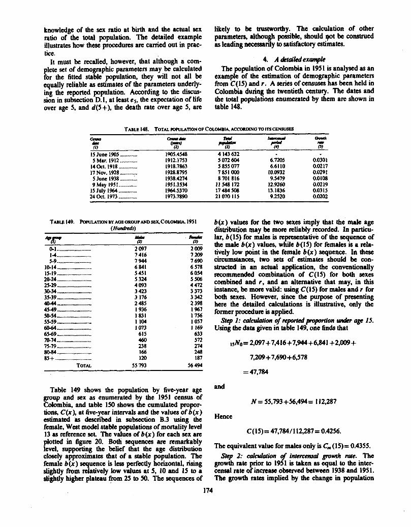
Tlrs~e 149. POWLATION BY AGE GROUP AND SEX, COU)MBI& 195 1 ( H w d d )

""6- xda .F#b @) (3)

0-1 ................................... 2 097 2009 14 ................................... 7 416 7 209 5-9-, --...... , ................ 7 944 7 690

10-14 - ................................. 6 841 6 578 15-19.. ................................. 5 451 6 054 20-24 ................................... 5 324 5506 25-29 - ............................... 4 093 4 472 30.34 .................................. 3 423 3 373 35-39 - ......... 1 ..................... 3 176 3 342 4044 ................... w .............. 2 485 2 398 4549 ................................... 1 936 1 967 50-54 ... " .............................. 1 831 1 756 55-59" ................................ 1 104 1 057 6064 ......................... - ........ 1 073 1 169 65-69 ., .............................. 615 633 70-74 ........... - ...................... 460 572 75-79 -.- .............................. 238 274

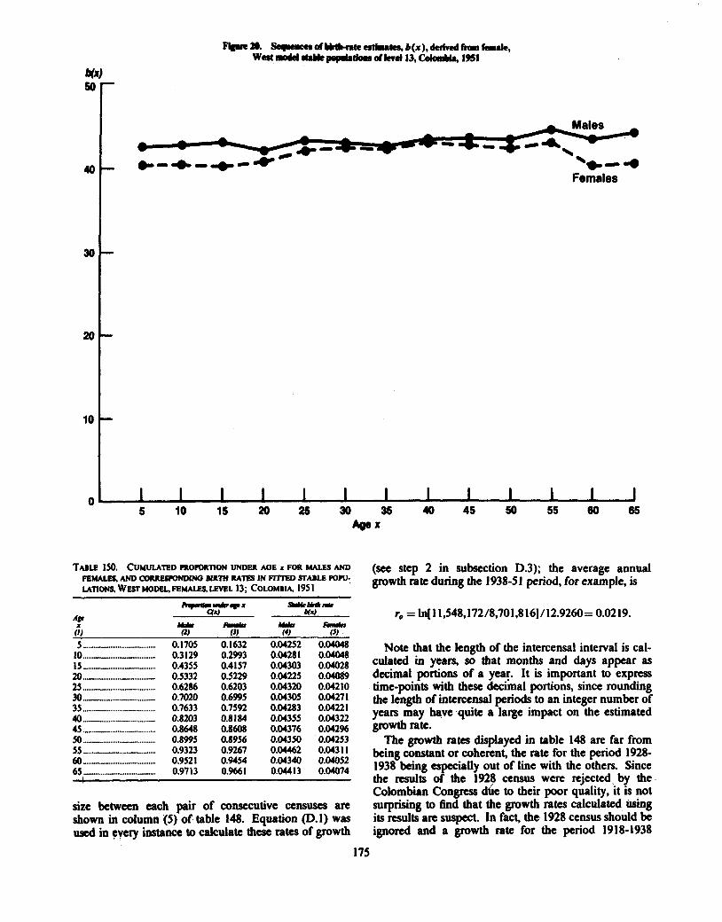
b(x) values for the two sexes imply that the male age distribution may be more reliably recorded. In particular, b(l5) for males is representative of the sequence of the male b(x ) values, while b(I5) for females is a relatively low point in the female b(x) sequence. In these circumstances, two sets of estimates should be con- structed in an actual application, the conventionally recommended combination of C(15) for both sexes combined and r , and an alternative that may, in this instance, be more valid: using C(15) for males and r for both sexes. However, sina the purpose of presenting here the detailed calculations is illustrative, only the former procedure is applied.

Step 1: caldhtion ~ m ~ p r o p o m m o n un&r agr 15. Using the data given in table 149, one finds that

Table 149 shows the population by five-year age group and sex as enumerated by the 1951 census of Colombia, and table 150 shows the cumulated proportions, C(x), at five-year intervals and the values of b(x) estimated as described in subsection B.3 using the female, West model stable populations of mortality level 13 as reference set. The values of b(x) for each sex are plotted in figure 20. Both sequences are remarkably level, supporting the belief that the age distribution closely approximates that of a stable population. The female b(x) sequence is less perfectly horizontal, rising slightly from relatively low values at 5, 10 and 15 to a slightly higher plateau from 25 to 50. The sequences of

and

Hence

The quivalent value for males only is C, (IS)= 0.4355. Step 2: arrliwhtion I# htemnsol p w t k rate. The

growth rate prior to 1951 is taken as qua1 to the intercensal rate of increase observed between 1938 and 195 1. The growth rates implied by the change in population

Figwe 20. Squaws dbtfth-mte crtiutcr, b(x), &cd tmm tauk, West model lPWc papatadom d Ievd 13, CokaWa, 1951

l a = 40 c-.c---(c.-~ Females

TABLE 1%. CUMULATED IRO~ORTION UND~R AOE r FOR MALES AND (set step 2 in subsection D.3); the average annual ~~~ AND cmmeswNDSNO M* IN - *IU: growth rate during the 1938-5 1 period, for example, is LATIONS WEST MODEL, FEMALES, LEVEL 13; COLOMBIA, 195 1

size between each pair of consecutive censuses arc shown in column (5) of table 148. Equation (D.l) was used in every instance to calculate these rates of growth

Note that the length of the intcrcensal interval is calculated in years, so that months and days appear as decimal portions of a yeq. It is important to express time-points with these decimal portions, since rounding the length of intercensal periods to an integer number of years may have quite a large impact on the estimated growth rate.

The growth rates displayed in table 148 are far from being constant or coherent, the rate for the period 1928- 1938 being especially out of line with the others. Since the results of the 1928 census were rejected by the Colombian Congress d6e to their poor quality, it is not surprising to find that the growth rates calculated using its results a n suspect. In fact, the 1928 census should be ignored and a growth rate for the period 1918-1938

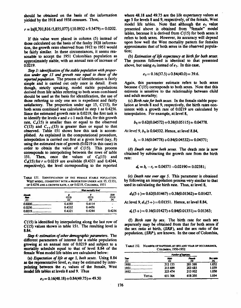
should be obtained on the basis of the information yielded by the 1918 and 1938 censuses. Thus,

If this value were placed in column (5) instead of those calculated on the basis of the faulty 1928 information, the growth rates observed from 1912 to 1951 would be fairly similar. In these circumstances, it seems rea- sonable to accept the 1951 Colombian population as approximately stable, with an annual rate of increase of 0.0219.

Step 3: i&ntification of the stable poplation with proportion d r age 15 Md growth rate equal to those of the ~ e d p o p d a t i o n . The process of identification is fairly simple and is carried out only once in detail. Even though, strictly speaking, model stable populations derived from life tables refemng to both sexes combined should be used as the basii for identification, the use of those refemng to only one sex is expedient and fairly satisfactory. The proportion under age 15, C(15), for both sexes combined was calculated in step 1 as 0.4256. Since the estimated growth rate is 0.0219, the first task is to identify the levels v and 9+ 1 such that, for this growth rate, C,(15) is smaller than or equal to the observed C(15) and C,+1(15) is greater than or equal to that observed. Table IS1 shows how this task is accom- plished. As explained in the computational procedure, interpolation is carried out first at a given level (say, 8) using the estimated rate of growth (0.0219 in this case) in order to obtain the value of C(15). This process corresponds to interpolating between the rows of table 151. Then, once the values of C8(15) and Cs(15) for r = 0.0219 are available (0.4321 and 0.4244, respectively), the level corresponding to the reported

where 48.18 and 49.75 arc the life expectancy values at age 5 for levels 8 and 9, respectively, of the female, West model life tables. Note that although the es value presented above is obtained from "female" model tables, because it is derived from C(15) for both sexes it refers to both sexes. However, its accuracy will depend upon how well the West mortality pattern for females approximates that of both sexes in the observed population;

(b) &timation of lfe expectancy at birth for both sexes. The process followed is identical to that presented above, but using eo instead of e5. in this cast,

Again, this parameter estimate refers to both sexes because C(15) corresponds to both sexes. Note that this estimate is sensitive to the relationship between child and adult mortality;

(c) Birth mte for both sexes. In the female stable population at levels 8 and 9, respectively, the birth rates consistent with a growth rate of 0.0219 are calculated by interpolation. For example, at level 8,

At level 9, b9 is 0.04532. Hence, at level 8.84,

(d) b h rate for both sexes. The death rate is now obtained by subtracting the growth rate from the birth rate:

TABLE 151. IDENTIFICATION OF THE FEMALE STABLE POPULATION. (e) &ath rate owr age 5. This parameter is obtained WEST MODEL CONSISTENT WITH A PROPORTION UNDER AGE 15, C( IS), by following an interpolation process very similar to that OF 0.4256 AND A GROWTH RATE. r, OF 0 . 0 2 19, COLOMBIA. 195 1 used in calculating the birth rate. Thus, at level 8,

w.* nayuy kul

on* 8 9 LM da(5 +) = 0.62(0.01467) +0.38(0.01362)= 0.01427. k* q.l9 q.l* cy.l>) (1) (2) (3) (4)

0.0200.-.,. ......-.. ............. 0 . 4 1 9 2 0 .41 1 4 At level 9, d9(5 +) =0.0135 1. Hence, at level 8.84,

C(15) is identified by interpolating along the last row of C(15) values shown in table 151. The resulting level is 8.84.

Srcp 4: estimation of other &mogqphicparameters. The different parameters of interest for a stable population growing at an annual rate of 0.0219 and subject to a mortality schedule equal to that of level 8.84 of the female West model life tables are calculated below:

(a) lEjrpctation of life at age 5, both sexes. Using 8.84 as the representative level, e5 may be estimated by interpolating between the e~ values of the female, West model life tables at levels 8 and 9. Thus

( f ) Birth m e by sex. The birth rate for each sex separately may be obtained from that for both sexes if the sex ratio at birth, (SRB), and the sex ratio of the population, (SRP), are known. In the case of Colombia,

TABLE 152. NUMBER OF BAPTISMS. BY SEX AND YEAR OF OCCURRENCE, COLOMBIA 1950-1952

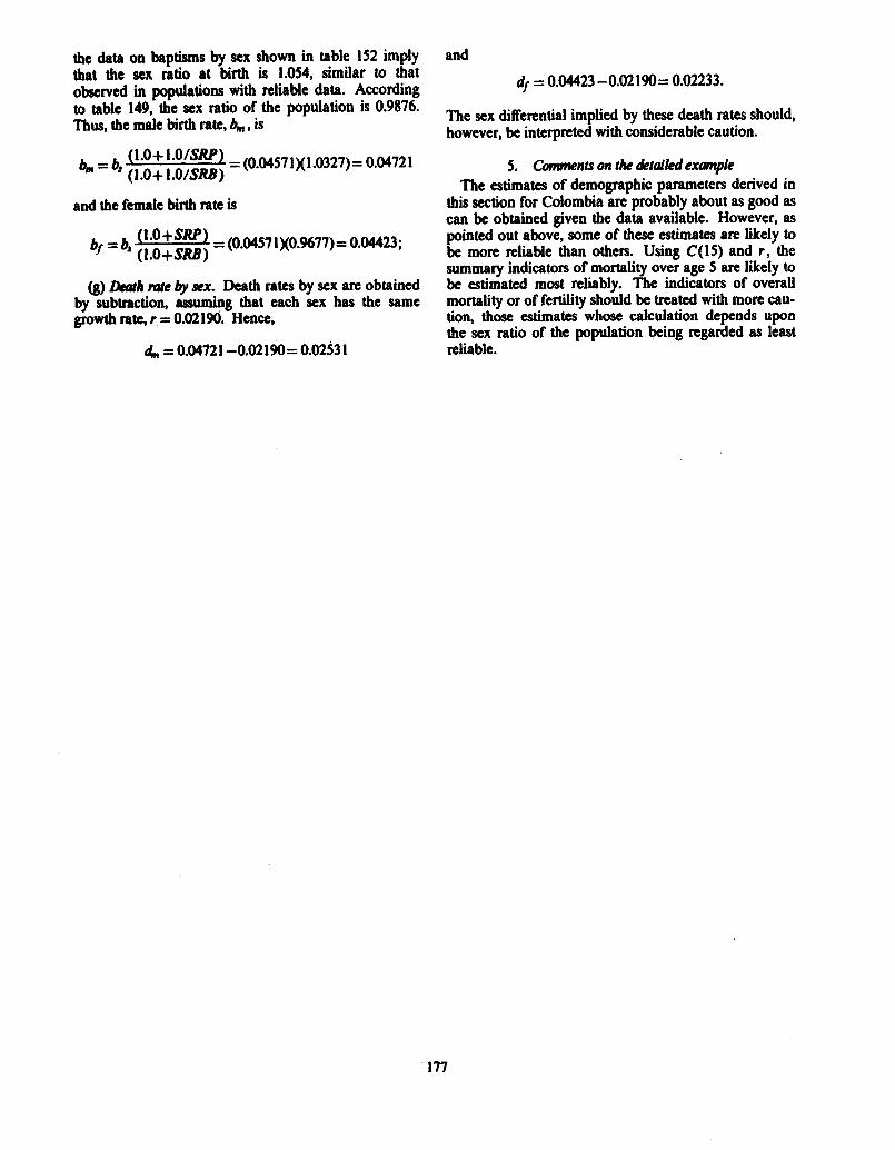
the data on baptisms by sex shown in table 152 imply that the sex ratio at birth is 1.054, similar to that observed in populations with reliable data. According to table 149, the sex ratio of the population is 0.9876. Thus, the male birth rate, 6, , is

and the female birth rate is

(8) Lkwth rate by sex. Death rates by sex are obtained by subtraction, assuming that each sex has the same growth rate, r = 0.02 1W. Hence,

and

The sex differential implied by these death rates should, however, be interpreted with considerable caution.

5. Gmments on the detailed example The estimates of demographic parameters derived in

this section for Colombia are probably about as good as can be obtained given the data available. However, as pointed out above, some of these estimates are likely to be more reliable than others. Using C(15) and r , the summary indicators of mortality over age 5 are likely to be estimated most reliably. The indicators of overall mortality or of fertility should be treated with more caution, those estimates whose calculation depends upon the sex ratio of the population being regarded as least reliable.

fertility and mortality estimation using model stable age distributions

Documents