feynman™s path integral approach to quantum field … · feynman™s path integral approach to...
TRANSCRIPT
FEYNMAN�S PATH INTEGRAL APPROACH TO QUANTUM FIELD THEORY
c William O. Straub, PhDPasadena, California
April 2004
�Consider the lilies of the goddamn �eld.��Ulysses Everett McGill, O Brother, Where Art Thou?
Here�s an elementary explanation of the mathematics behind Feynman�s path integral, along with a verysimpli�ed overview of its application to self-interacting quantum �eld theory (QFT), also known as �4 scalar�eld theory. Although it�s elementary, there�s enough information to provide a basic understanding of whatthe path integral is and how it leads to a many-particle interpretation in QFT. The discussion is very detailedin some of the �ner points, and some of the material is just plain overkill, so it�s rather longer than I wanted.But if you can stand my frankly insu¤erable didactic style, it may help you �ll in the blanks.
NotationMost of the integrals in QFT are four dimensional, but for brevity I have used dx in lieu of d4x wheneverpossible. Similarly, dk and k are four dimensional (although occasionally k is the 3-momentum), while kxis shorthand for k�x�. The Dirac delta function is denoted as �
4(x), which may occasionally look like thefourth-power functional derivative operator �4=�J4, so don�t get them confused. Unless speci�ed otherwise,integration limits are �1 to +1: Einstein�s summation convention is assumed, as is Dirac notation.
PrerequisitesFor basic background material on quantum mechanics, I very strongly recommend that you read J.J. Sakurai�sModern Quantum Mechanics, which is probably the best book on the subject at the advanced undergraduateor beginning graduate level. The �rst few chapters provide an especially clear overview of the basic principles,with emphasis on the mathematical notation I use here (the so-called Dirac notation), along with Sakurai�sextremely lucid exposition on quantum dynamics. As a student, I didn�t like Sakurai�s book much at �rstbecause I didn�t want to work with Dirac notation and because Sakurai seemed to leave out too many stepsin his derivations. Now I cannot imagine anyone learning quantum theory without his book. At the sametime, I cannot imagine how anyone could learn anything from Dirac�s Principles of Quantum Mechanics �itseems ancient, dry and boring to me, even though it was written (in my opinion) by the greatest theoreticalphysicist who ever lived. But if Sakurai isn�t your cup of tea, try the second edition of R. Shankar�s Principlesof Quantum Mechanics, which is probably just as good and devotes two chapters to path integrals to boot.
As for QFT itself, there are many books available, all of them somewhat di¢ cult and obtuse, in my opinion(this is most likely because I�m an engineer, and there are many aspects of QFT that strain my logicalabilities). The best advice I can give you is to �nd a text that speaks to you at your level, then trymore advanced subjects as your con�dence increases. For me, L. Ryder�s Quantum Field Theory is aboutas comprehensible as they come, and I would recommend it as a starting point. It has a very readableintroduction to the Lagrangian formulation and canonical quantization, the latter of which should be readso that the reader will fully appreciate how much simpler the path integral approach is. Another relativelyunderstandable text is M. Kaku�s Quantum Field Theory, although the notation is occasionally a tri�e bizarre(for example, he expresses the closure relation as jpi
Rdp hpj = 1). If you�re desperate to learn QFT, and the
above books are still over your head, then try A. Zee�s excellent book Quantum Field Theory in a Nutshell.The author practically takes you by the hand for the �rst 60 pages or so, and if that doesn�t do the trick foryou then you�re probably a hopeless case.
Understanding the path integral is a snap, but picking up quantum �eld theory is a di¢ cult task. It�ssomewhat like learning a new language; it takes a while, but soon it starts to make sense, and then thingsget much easier. I hope you have a great deal of intellectual curiosity, because in the end that�s the mainthing that will motivate you to learn it. Hopefully, you�ll also learn to appreciate what a truly strange andwonderful world God created for us undeserving and witless humans. Good luck!
1
1. Derivation of the Propagator In Quantum MechanicsIn order to derive Feynman�s path integral, we �rst need to develop the concept of the propagator in quantumdynamics using the time translation operator U(t). To do this we shall need to review the distinction betweenoperators in the Schrödinger and Heisenberg �pictures.�
In the so-called Schrödinger operator picture, state vectors are assumed to be time-dependent, whereasoperators are taken as time-independent quantities. In this picture, all time dependence is assumed to comefrom the �moving� state ket j�; ti, while operators stay �xed in time. Even the Hamiltonian operator Hnormally is not itself dependent on time, but instead operates on state vectors whose time-dependent parts�feel�the e¤ect of H.
In elementary quantum dynamics, we de�ne the time translation operator U(t00; t0), which takes the valuethat some state ket j�; t0i has at time t0 and returns the value that the ket would have at time t00; thus,
j�; t00i = U(t00; t0) j�; t0i , where
U(t00; t0) = exp[�iH(t00 � t0)=�h]
(Please note that I�m going to drop the hat notation on the U and H operators from here on out.) Similarly,a state bra changes according to
h�; t00j = h�; t00jUy(t00; t0)where Uy(t00; t0) is the hermitian adjoint of U (I suppose that in this case, the quantity U(t00; t0) voids ourde�nition of a Schrödinger operator as being strictly time-independent, but we�ll have to overlook this fornow).
Now consider h�; t0j�; t0i. If the state vector is normalized, this quantity is unity. Obviously, if we evaluatethis quantity at some other time t00 nothing changes; that is,
h�; t00j�; t00i = h�; t0jUy(t00; t0)U(t00; t0) j�; t0i= h�; t0j�; t0i
(Actually, this holds trivially for any unitary operator, since the product of the operator and its adjoint isunity.) But now let�s see how the situation changes when we look at the expectation value of some operatorA, which we denote as h�; t0jAj�; t0i. At time t00, this goes over to
h�; t00jAj�; t00i = h�; t0jUy(t00; t0) A U(t00; t0) j�; t0i= [ h�; t0jUy] A [U j�; t0i ] (1.1)
= h�; t0j [UyAU ] j�; t0i (1.2)
Notice that we have used the associativity law of operator multiplication to write this in two ways. In (1.1),the operator A is sandwiched between time-translated state vectors, while in (1.2) the product operator UyAUappears wedged between unchanged state kets. The �rst situation (where the operator A is time-independent)corresponds to the Schrödinger picture, whereas the second involves the time-dependent Heisenberg operatorUyAU operating on the state vector j�; t0i, which keeps whatever value it has at time t0 for all time. Wetherefore have two ways of looking at dynamical systems, either of which is completely valid:
Schrödinger Picture : A is static, j�; t0i �! j�; t00iHeisenberg Picture : j�; t0i is static, A �! UyAU
We now need to look at how eigenkets change in the Heisenberg picture. First, let�s rename the time-independent operator A as AS , where S stands for Schrödinger. Similarly, the quantity UyAU is renamedAH for the obvious reason. We then have
AH = UyASU
Now let�s right-multiply both sides of this by the quantity Uyjaii, where jaii is a base ket of the operatorAS . We get
AH Uyjaii = UyASUU
yjaii= UyAS jaii= aiU
yjaii
2
Evidently, the quantity Uyjaii is the base ket in the Heisenberg picture, and the eigenvalue ai is the samein both pictures. Consequently, even though state vectors are considered time-independent in this picture,the base kets are not. To summarize, we have, in the Heisenberg picture,
jai; t00i = Uy(t00; t0)jai; t0i and
hai; t00j = hai; t0jU(t00; t0)
where U(t00; t0) = exp[�iH((t00 � t0)=�h]. Thus, the situation is reversed from what you�d normally expect�we don�t operate with U(t00; t0) on a base ket, we use Uy(t00; t0) instead to get the time-translated version.That�s all there is to it.
If you�re confused, please try to think of it this way: the operator Uy(t00; t0) replaces the t0 it �nds in aneigenket to its right with t00, while the operator U(t00; t0) does exactly the same thing to an eigenbra to itsleft. If a base ket or bra doesn�t specify any t (for example, jaii), then it�s assumed that t0 = 0. In that case,U(t00; 0) = U(t00), which replaces t = 0 with t = t00, etc.
Now let�s do something interesting with all this. For any state ket j�; t0i, we have as usual
j�; t00i = exp[�i=�hH(t00 � t0)]j�; t0i
The operator thus moves the state ket from its value at t0 to the value it would have at time t00 (we assumet00 > t0). We now move over to the Heisenberg picture. Let�s multiply the above ket by the position eigenbrahx00j (note that t0 = 0 is assumed here). We then get
hx00 j�; t00i = hx00j exp[�i=�hH(t00 � t0)] j�; t0i= hx00j exp[�i=�hH t00] exp[i=�hH t0] j�; t0i= hx00jU(t00)Uy(t0)j�; t0i= hx00; t00jUy(t0) j�; t0i
Notice how U(t00) found a bra to its left with t = 0 and stuck t00 into it. We now insert the closure relationZdx0 jx0ihx0j = 1
immediately to the right of Uy(t0) and write this as
hx00j�; t00i =Zdx0 hx00; t00jUy(t0)jx0ihx0j�; t0i
Again, the Heisenberg picture changes this to
hx00j�; t00i =Zdx0 hx00; t00jx0; t0ihx0j�; t0i
Now, you might recall that the wave function is just �(x; t) = hxj�; ti, so this can be expressed simply as
�(x00; t00) =
Zdx0 hx00; t00jx0; t0i�(x0; t0) (1.3)
How do we interpret this? Whatever the quantity hx00; t00jx0; t0i is, it acts kind of like the double Dirac deltafunction �3(x00 � x0) �(t00 � t0). In fact, for t00 = t0 it is precisely the delta function �3(x00 � x0). However,when t00 6= t0 we give it the name propagator. The propagator hx00; t00jx0; t0i is actually a Green�s functionthat determines how the wave function develops in time and space (it�s often written as K(x00; t00;x0; t0);which to me detracts from the Dirac notation we�ve been using). It can (and should) be viewed as theprobability amplitude for a particle located originally at x0; t0 to be found at x00; t00 (remember that wealways read probability amplitudes from right to left, like Hebrew or Arabic). In anticipation of where thisis all going, I�ll mention here that the propagator can easily be extended to the case of a quantum �eldpropagating from one state to another. For example, in the path integral approach to quantum �eld theory,
3
the propagator h0;1j0;�1i expresses the amplitude of the vacuum state �j0i� to transition from minusin�nity back to itself in the distant future via an in�nite number of non-vacuum states involving particlecreation and annihilation.
Note also that the propagator can be broken into multiple steps; that is,
hxn; tnjx0; t0i � hxn; tnjx; ti hx; tjx0; t0i
where the spacetime point x; t is intermediate between x0; t0 and xn; tn. Obviously, we can promote this tothe equality
hxn; tnjx0; t0i =Zdx hxn; tnjx; ti hx; tjx0; t0i
where we have used a closure relation to link the two propagators. We can do this again and yet again:
hxn; tnjx0; t0i =ZZZ
dx1 dx2 dx3 hxn; tnjx3; tihx3; tjx2; tihx2; tjx1; ti hx1; tjx0; t0i
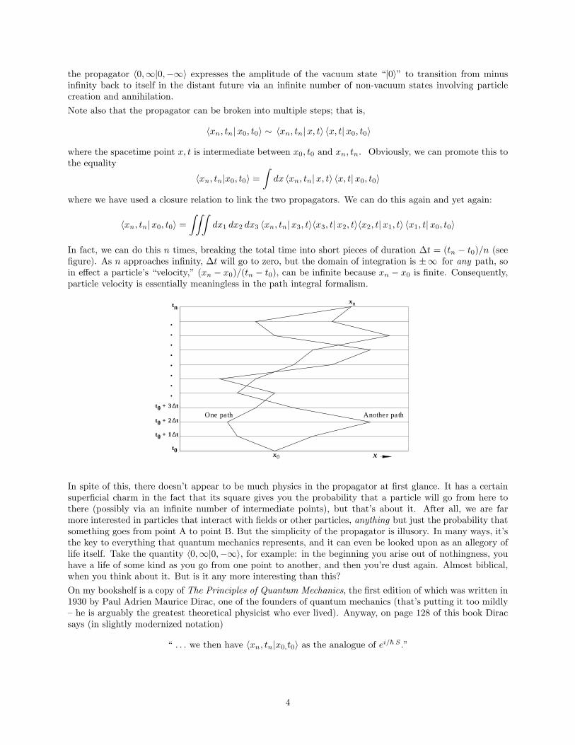
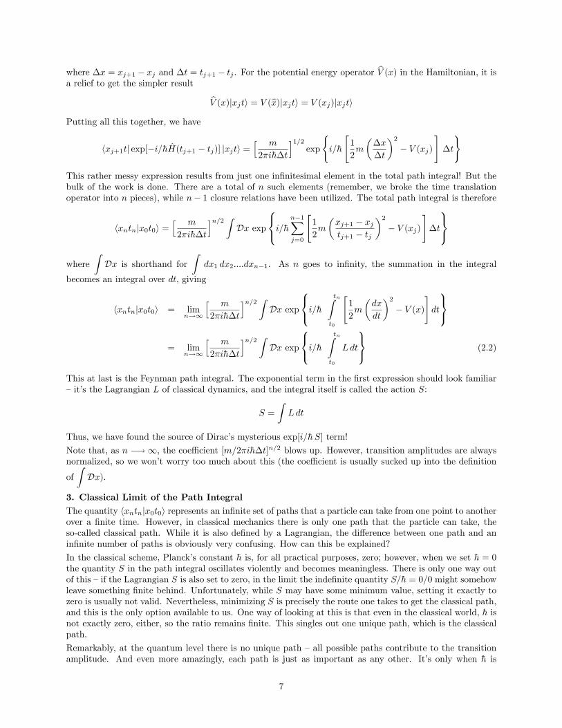
In fact, we can do this n times, breaking the total time into short pieces of duration �t = (tn � t0)=n (see�gure). As n approaches in�nity, �t will go to zero, but the domain of integration is �1 for any path, soin e¤ect a particle�s �velocity,� (xn � x0)=(tn � t0), can be in�nite because xn � x0 is �nite. Consequently,particle velocity is essentially meaningless in the path integral formalism.
t0
One path Another path
x0
xn
t0 + 1 ∆t
t0 + 2 ∆t
t0 + 3 ∆t
tn
.
.
.
.
.
.
.
.
x
In spite of this, there doesn�t appear to be much physics in the propagator at �rst glance. It has a certainsuper�cial charm in the fact that its square gives you the probability that a particle will go from here tothere (possibly via an in�nite number of intermediate points), but that�s about it. After all, we are farmore interested in particles that interact with �elds or other particles, anything but just the probability thatsomething goes from point A to point B. But the simplicity of the propagator is illusory. In many ways, it�sthe key to everything that quantum mechanics represents, and it can even be looked upon as an allegory oflife itself. Take the quantity h0;1j0;�1i, for example: in the beginning you arise out of nothingness, youhave a life of some kind as you go from one point to another, and then you�re dust again. Almost biblical,when you think about it. But is it any more interesting than this?
On my bookshelf is a copy of The Principles of Quantum Mechanics, the �rst edition of which was written in1930 by Paul Adrien Maurice Dirac, one of the founders of quantum mechanics (that�s putting it too mildly�he is arguably the greatest theoretical physicist who ever lived). Anyway, on page 128 of this book Diracsays (in slightly modernized notation)
� : : : we then have hxn; tnjx0;t0i as the analogue of ei=�hS .�
4

Here, Dirac�s S is the familiar action quantityRLdt, where L(x; _x; t) is the Lagrangian of classical mechanics.
Now, how does this come about? The Lagrangian has everything built into it �kinetic and potential energy,including interaction terms �so if Dirac�s remark is true, then the propagator is truly a wonderful discovery.Could it be that a principle of least action holds in quantum mechanics (as it does in classical mechanics),such that by minimizing S the quantity hxn; tnjx0;t0i will describe the true path of a particle? As a younggraduate student at Princeton University, Richard Feynman is said to have been fascinated by this ratherbrusque, throw-away remark by Dirac. What did Dirac mean by �analogue,�and how does the Lagrangianenter into it, anyway? (Dirac made a similar remark in a seminal paper he published in 1933 [apparently,this is the one Feynman was intrigued by]; see the references). To make a long story short, Feynman tookthe idea and made it the basis of his 1942 PhD dissertation (The Principle of Least Action in QuantumMechanics), and in doing so discovered a completely new approach to quantum theory �the path integral.You can do it, too �just recognize that hxn; tnjx0;t0i = hxnjU(tn � t0)jxi, and remember that U containsthe Hamiltonian operator H, which provides all the physics. Getting the ei=�hS term out of this is just onestep in what all physicists consider to be one of the most profound discoveries of quantum physics �the pathintegral approach to quantum �eld theory.
2. Derivation of the Path IntegralLet us write the Heisenberg-picture propagator as hxn tnjx0 t0i, which represents the transition amplitudefor a particle to move from the point x0 at time t0 to some other point xn at another time tn(again, assumetn > t0). In this picture, we�ll use the shorthand notation
hxn tnjx0 t0i � hnj0i = hxn tj exp[�i=�hH(tn � t0)] jx0 ti
Remember that the two t�s on the right hand side are completely arbitrary, because the time translationoperator is going to replace them with tn and t0. In most texts, they�re not even shown.
Let�s now split the time up into n equal pieces by setting �t = (tn � t0)=n. We can then write the timetranslation operator as the n-term product
exp[�i=�hH(tn � tn�1)] exp[�i=�hH(tn�1 � tn�2)] : : : exp[�i=�hH(t2 � t1)] exp[�i=�hH(t1 � t0)]
where tj+1 � tj = �t; j = 0; 1; 2 :::n � 1. We now insert a position eigenket closure relation just before thelast exponential term:
hnj0i =Zdx1 hxntjexp[�i=�hH�t]| {z }
n�1 times
jx1 tihx1 tj exp[�i=�hH(t1 � t0)] jx0ti
(where the time t is arbitrary and the limits of integration are from �1 to 1). The last term is
hx1tj exp[�i=�hH(t1 � t0)] jx0ti = hx1t1jx0t0i
The integral over dx1 means summation over every possible spacetime point along the t = 1 time step, so ine¤ect we are integrating over every possible path between t0 and t1.
Let�s repeat this procedure by inserting another closure relationRdx2jx2tihx2tj just to the left of the next
exponential operator. Using
hx2tj exp[�i=�hH(t2 � t1)] jx1ti = hx2t2jx1t1i
we now have
hnj0i =ZZ
dx1dx2 hxntjexp[�i=�hH�t]| {z }n�2 times
jx2tihx2t2jx1t1ihx1t1jx0t0i
The integrals over x1 and x2 mean that every path between t0 and t2 has been accounted for. Continuingthis process of closure insertion a total of n� 1 times, we have
hnj0i =Zdx1dx2 : : : dxn�1 hxnjxn�1tn�1ihxn�2tn�2jxn�3tn�3i : : : hx1t1jx0t0i (2.1)
5

where the single integral sign is now shorthand for an n � 1-dimensional integral (please note that we arenot integrating over the initial and �nal points). This simply shows that the propagator hxntnjx0t0i can beexpressed as the product of smaller propagator terms, as I indicated earlier. No big surprise here, and youmay think that it is all a big waste of time and e¤ort to write this as an n� 1-dimensional integral, which at�rst glance appears impossible to evaluate anyway. What we have then in the above integral is an expressionfor taking n � 1 paths to get from the starting point to the end, where each path is itself integrated overevery time step �t.
Of course, you can see what�s going to happen �we�re going to let n go to in�nity, which means that wewill consider all possible paths in the complete propagator, which includes every possible point in spacetimefrom the starting point 0 to the end point n. We will do this not to make life more di¢ cult, but to seewhat happens when we retain the exponential terms exp[�i=�hH�t]; naturally, the time step will now go like�t �! dt. I regard the fact that we can carry this out in a (mostly) mathematically unambiguous manneras nothing short of a miracle.
As indicated earlier, the physics in all this lies in the Hamiltonian H, which describes just about anyproblem, from the free particle to the hydrogen atom and beyond. The exponential terms containing H inthe last expression disappeared, but only so that the propagator could be expressed as a product term ofmany smaller propagators. Now we will see what Feynman discovered back in his days as a young graduatestudent at Princeton.
Let us pick a typical term in the above integral:
hxj+1tj+1jxjtji = hxj+1tj exp[�i=�hH(tj+1 � tj)] jxjti
We�re going to express H in its most familiar form, H = p2=2m + V (x), where the little hats as usual meanthat the quantities are operators. This is not relativistic, of course, but it will serve our purposes for thetime being. Let�s deal with the momentum operator term �rst. Since jxj ti is a position eigenket, we needsomething for the momentum operator p to �hit,�so we insert a momentum closure relation (again, all limitsare � in�nity) and rewrite this as the integral
hxj+1tj+1jxjtji =Zdp hxj+1tj exp[�i=�hH(tj+1 � tj)] jpihpjxjti
But this is justZdp hxj+1tj exp[�i=�hH(tj+1 � tj)] jpihpjxjti =
Zdp hxj+1tjpihpjxjti exp[�i=�hp2=2m (tj+1 � tj)]
where the p term in the exponential is no longer an operator. From any basic quantum mechanics text, welearn that
hxj+1jpi =1p2��h
exp[i=�h pxj+1]
andhpjxji =
1p2��h
exp[�i=�h pxj ]
both which hold for any t. We then haveZdp hxj+1tjpihpjxjti exp[�i=�hp2=2m (tj+1�tj)] =
1
2��h
Zdp exp
�i=�h
�p(xj+1 � xj)� i=�hp2=2m (tj+1 � tj)
�This is a Gaussian integral, and it can be solved exactly once we complete the square in the exponential term(you should be happy to know that the high school algebra exercise of �completing the square�actually hasa practical use). To save time, I�ll just write down the answer:
hxj+1tj exp[�i=�hH(tj+1 � tj)] jxjti =h m
2�i�h�t
i1=2exp
"i=�h
1
2m
��x
�t
�2�t
#
6
where �x = xj+1 � xj and �t = tj+1 � tj . For the potential energy operator bV (x) in the Hamiltonian, it isa relief to get the simpler result bV (x)jxjti = V (bx)jxjti = V (xj)jxjti
Putting all this together, we have
hxj+1tj exp[�i=�hH(tj+1 � tj)] jxjti =h m
2�i�h�t
i1=2exp
(i=�h
"1
2m
��x
�t
�2� V (xj)
#�t
)This rather messy expression results from just one in�nitesimal element in the total path integral! But thebulk of the work is done. There are a total of n such elements (remember, we broke the time translationoperator into n pieces), while n� 1 closure relations have been utilized. The total path integral is therefore
hxntnjx0t0i =h m
2�i�h�t
in=2 ZDx exp
8<:i=�hn�1Xj=0
"1
2m
�xj+1 � xjtj+1 � tj
�2� V (xj)
#�t
9=;where
ZDx is shorthand for
Zdx1 dx2::::dxn�1. As n goes to in�nity, the summation in the integral
becomes an integral over dt, giving
hxntnjx0t0i = limn!1
h m
2�i�h�t
in=2 ZDx exp
8<:i=�htnZt0
"1
2m
�dx
dt
�2� V (x)
#dt
9=;= lim
n!1
h m
2�i�h�t
in=2 ZDx exp
8<:i=�htnZt0
Ldt
9=; (2.2)
This at last is the Feynman path integral. The exponential term in the �rst expression should look familiar�it�s the Lagrangian L of classical dynamics, and the integral itself is called the action S:
S =
ZLdt
Thus, we have found the source of Dirac�s mysterious exp[i=�hS] term!
Note that, as n �! 1, the coe¢ cient [m=2�i�h�t]n=2 blows up. However, transition amplitudes are alwaysnormalized, so we won�t worry too much about this (the coe¢ cient is usually sucked up into the de�nition
ofZDx).
3. Classical Limit of the Path IntegralThe quantity hxntnjx0t0i represents an in�nite set of paths that a particle can take from one point to anotherover a �nite time. However, in classical mechanics there is only one path that the particle can take, theso-called classical path. While it is also de�ned by a Lagrangian, the di¤erence between one path and anin�nite number of paths is obviously very confusing. How can this be explained?
In the classical scheme, Planck�s constant �h is, for all practical purposes, zero; however, when we set �h = 0the quantity S in the path integral oscillates violently and becomes meaningless. There is only one way outof this �if the Lagrangian S is also set to zero, in the limit the inde�nite quantity S=�h = 0=0 might somehowleave something �nite behind. Unfortunately, while S may have some minimum value, setting it exactly tozero is usually not valid. Nevertheless, minimizing S is precisely the route one takes to get the classical path,and this is the only option available to us. One way of looking at this is that even in the classical world, �h isnot exactly zero, either, so the ratio remains �nite. This singles out one unique path, which is the classicalpath.
Remarkably, at the quantum level there is no unique path �all possible paths contribute to the transitionamplitude. And even more amazingly, each path is just as important as any other. It�s only when �h is
7

comparatively small that the paths begin to interfere destructively, leaving a large propagation amplitudeonly in the vicinity of the classical path. When you studied the electron double-slit experiment, your professorno doubt informed you that each electron in reality passes through both slits on the screen on its way to thedetector and, in doing so, interferes with itself, which is why the detector shows an interference pattern. Fora triple slit, the electron has three possible routes, and there is a corresponding interference pattern. We canin fact make an in�nite number of slits in an in�nite number of sequential screens (leaving empty space!),and the electron will then be describable by Feynman�s path integral formalism. Fantastic as this may seem,the formalism appears to be a correct description of reality.
4. The Free Particle PropagatorThe real power of the path integral lies in the fact that it includes the interaction term V (x). We cantherefore (in principle) compute the amplitude of a particle that interacts with external �elds and otherparticles as it propagates from one place to another, an in�nite number of times, if necessary (which isnormally the case). Another advantage lies in the fact that the Lagrangian can accommodate any numberof particles, because we can always write
L =Xk
"1
2mk
�dxkdt
�2� V (xk)
#(4.1)
Consequently, the path integral can be applied to many-particle systems, making it a good candidate for aquantum �eld theoretic approach (in my opinion, it�s unequivocally the best and most natural approach). Youmay recall that quantum mechanics normally deals with only one or several particles, and gets progressivelymore di¢ cult as the number of particles becomes large. In quantum �eld theory, large numbers of particlesare par for the course.
What assurance do we have that the path integral in (2.2) represents reality? Well, we might try toactually compute one, hopeless though this appears at �rst glance. After all, a single integral may not bea problem, but computing an in�nite-dimensional integral might become tedious after a while. It turns outthat, for the case V (x) = 0, the path integral can be obtained in closed form. This leads us to the freeparticle propagator.
First let�s derive this quantity using ordinary quantum mechanics. It is simplicity itself. We write
hxntnjx0t0i = hxntj exp��i=�h p2=2m (tn � t0)
�jx0ti
=
Zdp hxntj exp
��i=�h p2=2m (tn � t0)
�jpihpjx0ti
=1
2��h
Zdp exp
�i=�h p(xn � x0)� i=�hp2=2m (t)
�This is the same Gaussian integral we evaluated earlier. The integration over p is elementary, and the freeparticle propagator turns out to be
hxntnjx0t0i =r
m
2�i�h(tn � t0)exp
�im
2�h(tn � t0)(xn � x0)2
�(4.2)
Well, that was easy enough. Can we reproduce this using the path integral? We can indeed, although thealgebra is a bit more involved. Let�s rewrite (2.2) as
hxntnjx0t0i =h m
2�i�h�t
in=2 ZDx exp
24� n�1Xj=0
a (xj+1 � xj)235
where
a = � im
2�h�t
Why did I write this so that a would have a negative sign? It�s because we want a decreasing exponentialto evaluate the Gaussian integrals that we will introduce next (the fact that a is pure imaginary completely
8
voids this argument, but what the hell). Now let�s focus on the �rst integral we�ll have to evaluate, which is
I1 =
Zexp
��a(x2 � x1)2 � a(x1 � x0)2
�dx1
(we�re starting from the far right-hand side of the integral string). This is a Gaussian integral, as promised,although the integration variable x1 is coupled with x0 and x2. Holding the latter two variables constant,the integration is straightforward, and we get
I1 =
r�
2aexp
��12a(x2 � x0)2
�Now we need to do the next integral, which looks like
I2 =
Zexp
��a(x3 � x2)2 �
1
2a(x2 � x0)2
�dx2
Again, this is just another Gaussian integral, though slightly di¤erent than the one we evaluated for I1.Holding x0 and x3 constant, this time around we get
I2 =
r2�
3aexp
��13a(x3 � x0)2
�I can keep doing this, but hopefully you�ve already spotted the pattern, which is
Ik =
sk�
(k + 1)aexp
�� 1
k + 1a(xk+1 � x0)2
�As a result, we get a chain of leading square root terms in the complete integration, which goes liker
1�
2a
r2�
3a
r3�
4a: : : �! 1p
n
h�a
i(n�1)=2(The n�1 term results from the fact that we�re doing a total of n�1 integrals.) Putting everything together(including the (m=2�i�h�t)n=2 term), we have �nally
hxntnjx0t0i =h m
2�i�h�t
in=2 1pn
h�a
i(n�1)=2exp
�� 1na (xn � x0)2
�=
h m
2�i�hn�t
i1=2exp
�im
2�hn�t(xn � x0)2
�where we have inserted the de�nition for a into the second expression. Lastly, we set n�t = tn � t0, leavingus with
hxntnjx0t0i =r
m
2�i�h(tn � t0)exp
�im
2�h(tn � t0)(xn � x0)2
�which is the free particle propagator again! Although the e¤ort was enormous, the path integral has du-plicated a result from quantum mechanics (let this simple example be a lesson to you � computing pathintegrals is no fun). This happy outcome indicates that the path integral approach seems to work, eventhough it is an entirely di¤erent way of looking at things. Furthermore, we now have greater con�dence thatthe path integral approach will be valid even when the potential term V (x) is retained. Indeed, for simplesystems like the harmonic oscillator, the path integral approach exactly replicates the results of quantummechanics (I won�t do that one here, as this discussion is already long enough). We are now ready to makethe big leap from quantum mechanics to quantum �eld theory using Feyman�s path integral.
5. The Path Integral Approach to Quantum Field TheoryThe transition from quantum mechanics to quantum �eld theory is straightforward, but the underlying
concept is a little di¢ cult to grasp (at least it was for me). Basically, three issues must be dealt with.
9
One, we demand that the theory be dynamically relativistic (in other words, E = p2=2m+ V must be giventhe axe). Two, space and time variables must share equal billing; this is just another relativistic demand.In quantum mechanics, time is just a parameter whereas position is an operator (that�s why we see thingslike jxi, whereas the object jti is nonsensical). And third, quantum mechanics is primarily a one-particletheory, while a quantum �eld theory we must somehow accommodate many particles (to account for particlecreation and destruction). The path integral ful�lls all of these requirements admirably.
Now here�s the big leap in a nutshell: quantum �eld theory replaces the position coordinate x with a �eld�(x), where the quantity x is now shorthand for x, y, z, t. That is, dimensional coordinates are downgradedfrom operators to parameters, just like t, so everything�s on the same footing (in relativity, space and timeare conjoined into spacetime). This process of coordinate reassignment is known as second quantization.To reiterate (this is very important), we must have a quantity whose functions are x; y; z and t, somethinglike the wave function (�!x ; t). In quantum �eld theory, we assume the existence of a quantum �eld �(x)which may also include speci�cations concerning particle spin, particle number, angular momentum, etc. Inwhat is known as canonical �eld theory, the �eld itself is an operator (path integrals thankfully avoid thiscomplication). If all of this makes sense to you (and even if it doesn�t), then it shouldn�t surprise you thatwe can write the path integral in quantum �eld theory as
Z =
Z 1
�1D� exp
�i
�h
Z 1
�1L(�; x�; @��) d
4x
�(5.1)
where we assume that any and all coe¢ cients (nasty or otherwise) are now lumped into the D� notation,which goes like �(x1)�(x2) : : :. Why it�s called Z is just convention. You might want to think of this quantityas the transition amplitude for a �eld to propagate from the vacuum at t = �1 to the vacuum again att = 1, but I�m not sure that this prescription really describes it. A �eld can be just about anything, butyou can look at it in this situation as a quantity that might describe a population of particles, energy �eldsand/or force carriers at every point in spacetime. Also, it is no longer appropriate to call (5.1) a pathintegral, since it does not describe the situation in terms of paths in spacetime anymore. It is now called theZ functional integral.
You might now be wondering what the boundaries of the �eld are in terms of its possible values. Well, we cansingle out one very special �eld �the so-called vacuum state �in which the energy density of spacetime inthe vicinity of the system being considered is a minimum (usually zero), so that Z � j0i. By this we mean astate such that the modulus of the quantity Z cannot possibly assume any smaller value. By convention, weconsider a vacuum state which arises at t = �1, then propagates along as something other than a vacuumstate before returning to a vacuum �eld at t =1. In propagator language, we say that Z = h0, 1j0, �1i.In between these times, the �eld interacts with particles and other �elds (and even creates them) in a mannerprescribed by the Lagrangian. Thus, the �eld is born at t = �1, enjoys a �life�of some sort, and then diesat t =1 (that�s why both integrals in (5.1) go from minus to plus in�nity). Very simplistic, perhaps, but itseems to work alright in practice. By the way, this business of selecting the vacuum state as a starting pointis fundamental to what is to follow. Because the path integral with interaction terms cannot be evaluateddirectly, a perturbative approach must be used. Selection of the vacuum or �ground�state ensures that theperturbation method will not �undershoot�the vacuum and give sub-vacuum results, which are meaningless.If the true vacuum state is not assigned from the beginning, then the system may jump to states of evenlower energy. In QFT this would be a disaster, because (as we will see shortly) the method of solving forZ uses successive approximations (perturbation theory), and if we have a false vacuum, this method failsutterly. In fact, the Higgs process (which you may have read about) absolutely depends on �xing the truevacuum under a gauge transformation of the bosonic Lagrangian.
The form of the Lagrangian for a �eld depends on what kind of particles and force carriers are going tobe involved. Consequently, there are Lagrangians for scalar (spin zero) particles (also called bosons), spinors(spin 1/2 particles, also called fermions), and vector (spin one) particles. There�s even a messy one for spin-2gravitons. The simplest of these is the scalar or bosonic Lagrangian, and it is the one we will use here. Thescalar Lagrangian for relativistic �elds is given by
L =1
2[ @��@
���m2�2]� V
10
(for a derivation, see any intermediate quantum mechanics text).
Just like the ordinary propagator in quantum mechanics, we�re going to experience problems evaluatingZ when the potential term V is not a linear or quadratic function of its argument. As God would have it,the simplest interaction term for a scalar particle in quantum �eld theory turns out to be V � ��4, where �is called a coupling constant. This gives rise to what is called a self-interacting �eld theory; that is, the �eldinteracts with itself and with any particles that are created along the way. As a result, the integral for Zcannot be obtained in closed form, and we will have to resort to perturbation theory, as previously indicated.This leads to a very interesting interpretation of particle creation and propagation as a consequence of thismodel �at every order in the perturbative expansion (including zero order), particles appear and begin topropagate about the spacetime stage. Since in principle there is an in�nite number of spacetime points whereinteraction can occur, the number of particles involved can also be in�nite. However, the total number of allinteractions is �xed by the number of � that enter the perturbative expansion of Z.
So the problem comes down to solving the integral
Z(�) =
ZD� exp
�i
�h
Z �1
2
�@��@
���m2�2�� ��4
�d4x
�(5.3)
Alas, I will tell you right now that this integral cannot be attacked in this form. The main problem isthe in�nite-dimensional integral; it is simply too unwieldy. We will have to make some changes before aperturbative solution can be employed.
6. Modifying the Z Functional IntegralConsider the free-space (� = 0) form of Z with a �source�term J(x):
Z(J) =
ZD� exp
�i
Z �1
2
�@��@
���m2�2�+ J(x)�
�d4x
�(6.1)
which we will set to zero later (note that from here on, in keeping with the fashion standard in physics, I�msetting �h = c = 1 so I won�t have to carry them around everywhere). Although the introduction of J(x) intothe integral is a standard mathematical arti�ce, there is some physical justi�cation for it, but I won�t boreyou with the details. Integrating by parts over the @��@�� term, we getZ
1
2
�@��@
���m2�2�d4x = �
Z �1
2�@2�+
1
2m2�2
�d4x
Now assume that the �eld � can be written as
�(x) = �0(x) + '(x)
where �0 is the so-called �classical�solution to the heterogeneous equation
��@2 +m2
��0 = J (6.2)
and ' is the corresponding �1� 1��eld. The classical solution is unique (it corresponds to the classical�path�), but it�s just one of the in�nite identities the �eld can assume. Please don�t worry about that leadingminus sign; you can ignore it if you want, as it�s really not critical (I�m just following convention). Now, thesolution to (6.2) can be obtained using the usual method of Green�s functions:
��@2 +m2
�G(x� x0) = �4(x� x0) (6.3)
where G(x� x0) is the four-dimensional Green�s function associated with the operator ��@2 +m2
�. Then
�0(x) =
ZG(x� x0) J(x0) d4x0
is the desired solution (after all, this is what Green�s functions do for a living). To solve (6.3) for G(x� x0),we assume that it can be expressed as a Fourier transform
G(x� x0) =Z
d4k
(2�)4G(k) eik�(x
��x�0) (6.4)
11

where k is the momentum four-vector (E=c;�!p ). By hitting (6.4) with the operator ��@2 +m2
�, you should
be able to show that (6.3), along with the de�nition for the Dirac delta function
�4(x� x0) =Z
d4k
(2�)4eik�(x
��x�0)
leads to
G(k) =1
k2 �m2, so that (6.5)
G(x� x0) =
Zd4k
(2�)4eik�(x
��x�0)
k2 �m2and (6.6)
�0(x) =
ZG(x� x0) J(x0) d4x0 (6.7)
In scalar QFT, it is conventional to rename the Green�s function in (6.6) as the Feynman propagator �F (x�x0). At the same time, the momentum-space propagator (6.5), which is not an integral quantity, will be of uselater when we de�ne the so-called Feynman rules for a scattering process. [The above de�nition for G(x�x0)normally includes a �fudge factor�in the denominator (that is, k2 �m2 + i�) to help with convergence, butI will not use it just yet.] Anyway, we now have
�0(x) =
Z�F (x� x0) J(x0) d4x0; where
�F (x� x0) =
Zd4k
(2�)4eik(x�x
0)
k2 �m2
where kx means k�x�. That done, we can then write (6.1) as
Z(J) =
ZD' exp
�i
2
Z �@�'@
�'�m2'2�d4x�
ZZJ(x0)�F (x
00 � x0)J(x00) d4x0 d4x00�
Okay, now here�s the trick: J(x) appears under the integral, but it is an explicit function of the spacetimecoordinates x, and not a function of ', so the J integral term can be taken out of the in�nite-dimensionalintegral altogether :
Z(J) = exp
�� i2
ZZJ(x0)�F (x
0 � x00) J(x00) d4x0 d4x00� Z
D' exp�i
2
Z �@�'@
�'�m2'2��d4x
So just what is the residual integral over D'? Who knows, and who cares; it�s just some number, and youcan call it N if you want (like most textbooks), but I will set N = 1 because we�ll be using normalizedamplitudes later on. We then have, �nally,
Z(J) = exp
�� i2
ZJ(x)�F (x� x0) J(x0) dx dx0
�(6.8)
where I�m now using one integral sign and dx for brevity. Believe it or not, this is an enormous achievement,for we have successfully rid ourselves of that in�nite-dimensional integral and replaced it with two four-dimensional integrals. From here on out, everything we do will involve taking successive derivatives of Zwith respect to the J(x). This is the main reason why Z was �simpli�ed� in this way � it provides aparameter, J(x), with which the solution of Z(�) can now be straightforwardly developed.
7. Power Series Representation of the Z Functional Integral; Green�s FunctionsBecause we will have to resort to approximation to solve Z when the interaction term is included, it will behelpful to see how this quantity can be expressed as a power series expansion (more importantly, it servesas a means of introducing a form of Green�s function that is critical to the approximation scheme). Recall
12
that the series expansion of any two-variable function F (x; y) about zero can be written as
F (x; y) = F (0; 0) + x@F (x; y)
@xjx;y=0 + y
@F (x; y)
@yjx;y=0 +
1
2!xy
@2F (x; y)
@x @yjx;y=0 + : : :
=1Xn=0
nXm=0
1
n!xmyn�m
@nF (x; y)
@xm@yn�mjx;y=0
The extension of this formula to n variables is straightforward (but you�ll need n summation symbols!).By de�nition, a functional is a function of one or more functions. For a functional, the variables x and ybecome functions which we can expand out to a string of n quantities [say, s(x1); s(x2); : : : ; s(xn)] and thesummations become integrals over dx1dx2 : : : dxn, so the analogous expression for a functional looks like
F [s(x1); s(x2) : : : s(xn)] =1Xn=0
Z1
n!dx1dx2 : : : dxn s(x1) s(x2) : : : s(xn)Rn(x1; x2 : : : xn)
where
Rn(x1; x2 : : : xn) =
��
�s(x1)
�
�s(x2): : :
�
�s(xn)
�F [s]js=0
The operator � is what is known as the functional derivative operator. I�ll discuss this operator a little lateron, but for now all you need to know is that it more or less does to functionals (which are almost alwaysintegrals containing one or more functions of the integrating argument) what the ordinary partial derivativeoperator does to functions, except that:
@xi@xj
= �ij (the Kronecker delta)
�F (x)
�F (y)= �4(x� y) (the Dirac delta)
Believe it or not, the quantity Rn(x1; x2 : : : xn) is a kind of Green�s function, but in QFT it is called then-point function. We will see shortly that the n-point function is nonzero only for even n.In view of this, the functional Z(J) can be written as
Z(J) =
1Xn=0
Zin
n!dx1dx2 : : : dxn J(x1)J(x2) : : : J(xn)G(x1; x2 : : : xn)
where
G(x1;x2 : : : xn) =1
in
��
�J(x1)
�
�J(x2): : :
�
�J(xn)
�Z(J)jJ=0
The G functions pretty much de�ne the mathematical problem at hand, so if we know them then we knowZ. Therefore, knowing how to calculate them e¢ ciently is very important. Physicists have learned (or atleast they believe) that the quantities G(x1;x2 : : : xn) are the amplitudes for particles going from place toplace. For example, using (6.8) we can calculate the two-point function
G(x1;x2) =1
i2
��
�J(x1)
�
�J(x2)
�Z(J)jJ=0
= i�F (x1 � x2)
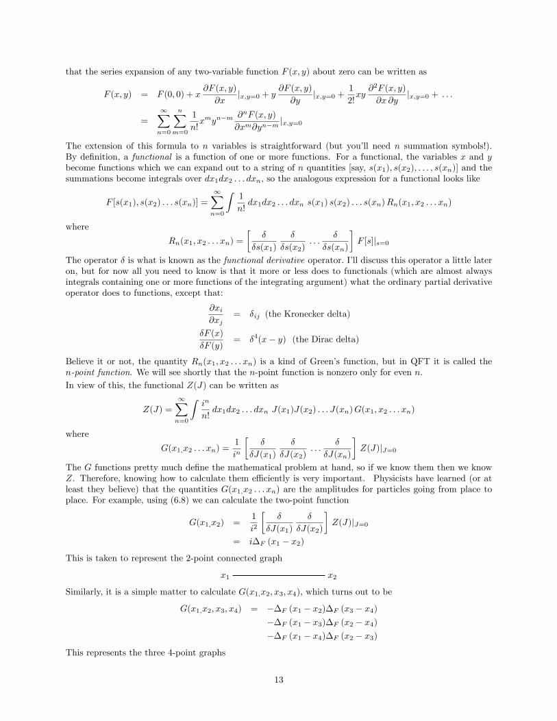
This is taken to represent the 2-point connected graph
x1 x2
Similarly, it is a simple matter to calculate G(x1;x2; x3; x4), which turns out to be
G(x1;x2; x3; x4) = ��F (x1 � x2)�F (x3 � x4)��F (x1 � x3)�F (x2 � x4)��F (x1 � x4)�F (x2 � x3)
This represents the three 4-point graphs
13
x3 x4
x1 x2
x3 x4
x1 x2
x3 x4
x1 x2
(Note that there are only three ways to connect the four points. This is basically what all these graphsinvolve �permutations of diagrams, connected up in every possible way.) I strongly urge you to calculateG(x1;x2; x3; x4) for yourself. Z is an exponential, so we can never run out of functional derivatives, no matterhow many of them we take. You will see that although it is straightforward, it�s somewhat tedious. Youwill learn that QFT can involve the calculation of Z(J) to many orders of xi, so we will have to �nd a wayof determining them without actually doing the calculations. Fortunately, there is a simple formula for thisthat you will learn later on.
Try to think of the G quantities as associated with particles that get created at some point (say, xi),propagate along a connecting line for a while [the line is represented by the quantity �F (xf �xi)], and thenget annihilated at a terminating point (xf ). The Feynman propagator �F is therefore the basic buildingblock of the n-point functions. Because the mathematics is described basically by points sitting on oppositesends of lines represented by �F , it should come as no surprise that these little points and lines are themselvesthe building blocks of what are known as Feynman diagrams. We will see that when the interaction term �gets involved, the lines will get attached only at points at which � occurs.
8. Interpretation of Z as a Generator of ParticlesFeynman recognized that this business of multiple Z di¤erentiations brings down terms that combine in waysthat are describable by simple graphs. Each term has a coe¢ cient associated with it that comes from thetopology of the associated diagram, and each term has a multiplicity that depends on the number of waysthat the diagram can be drawn. These amplitudes and multiplicities can be expressed mathematically usingcombinatorial algebra. We�ll get to that later. But �rst let�s have a look at those diagrams.
I�m going to show you how physicists interpret Z and how they associate diagrams with its expansion. Let�sstart with the free-space version,
Z(J) = exp
�� i2
ZZdx0dx00J(x0)�F (x
0 � x00) J(x00)�
(8.1)
Now replace each term in the integral with its Fourier counterpart (I�m retaining all the integral signs herefor accounting purposes):
Z(J) = exp
"� i2
1
(2�)12
ZZdx0dx00
ZZZdp0dp00dk J(p0) J(p00)
eix0p0eix
00p00eik(x0�x00)
k2 �m2
#
= exp
�� i2
1
(2�)4
ZZZdp0dp00dk J(p0) J(p00)
1
k2 �m2�4(p0 + k) �4(p00 � k)
�= exp
�� i2
1
(2�)4
Zdk J(k)
1
k2 �m2J(�k)
�(8.2)
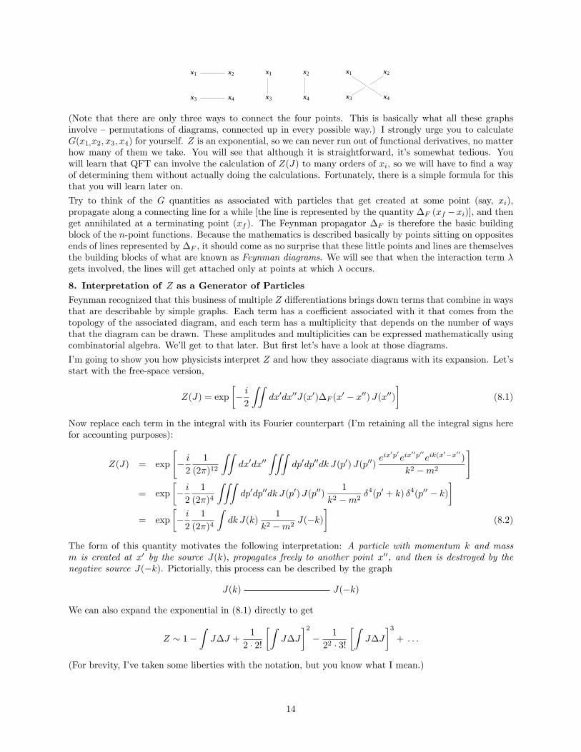
The form of this quantity motivates the following interpretation: A particle with momentum k and massm is created at x0 by the source J(k), propagates freely to another point x00, and then is destroyed by thenegative source J(�k). Pictorially, this process can be described by the graph
J(k) J(�k)
We can also expand the exponential in (8.1) directly to get
Z � 1�ZJ�J +
1
2 � 2!
�ZJ�J
�2� 1
22 � 3!
�ZJ�J
�3+ : : :
(For brevity, I�ve taken some liberties with the notation, but you know what I mean.)
14
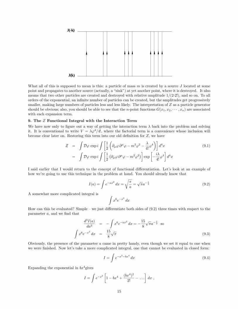
J(-k)
J(k)
What all of this is supposed to mean is this: a particle of mass m is created by a source J located at somepoint and propagates to another source (actually, a �sink�) at yet another point, where it is destroyed. It alsomeans that two other particles are created and destroyed with relative amplitude 1/(2�2!), and so on. To allorders of the exponential, an in�nite number of particles can be created, but the amplitudes get progressivelysmaller, making large numbers of particles less and less likely. The interpretation of Z as a particle generatorshould be obvious; also, you should be able to see that the n-point functions G(x1; x2; � � � ; xn) are associatedwith each expansion term.
9. The Z Functional Integral with the Interaction TermWe have now only to �gure out a way of getting the interaction term � back into the problem and solvingit. It is conventional to write V = �'4=4!, where the factorial term is a convenience whose inclusion willbecome clear later on. Restoring this term into our old de�nition for Z, we have
Z =
ZD' exp i
Z �1
2
�@�'@
�'�m2'2 � �
4!'4��
d4x (9.1)
=
ZD' exp i
Z �1
2
�@�'@
�'�m2'2��exp
�� i�4!'4�d4x
I said earlier that I would return to the concept of functional di¤erentiation. Let�s look at an example ofhow we�re going to use this technique in the problem at hand. You should already know that
I(a) =
Ze�ax
2
dx =
r�
a=p�a�
12 (9.2)
A somewhat more complicated integral is Zx6e�x
2
dx
How can this be evaluated? Simple �we just di¤erentiate both sides of (9.2) three times with respect to theparameter a, and we �nd that
d3I(a)
da3= �
Zx6e�ax
2
dx = �158
p�a�
72 soZ
x6e�x2
dx =15
8
p� (9.3)
Obviously, the presence of the parameter a came in pretty handy, even though we set it equal to one whenwe were �nished. Now let�s take a more complicated integral, one that cannot be evaluated in closed form:
I =
Ze�x
2�bx4 dx (9.4)
Expanding the exponential in bx4gives
I =
Ze�x
2
�1� bx4 + (bx
4)2
2!� : : :
�dx ;
15

so one approach to evaluating this is to use integral identities like (9.3) for all powers of x4. This will givea solution involving an in�nite number of terms, but if b is small we can always truncate the series at somepoint and obtain a solution that is as accurate as we want. But there�s another way of looking at this basicapproach. Let us write (9.4) without the x4 term but with another that is proportional to x:
I(c) =
Ze�x
2+cx dx (9.5)
Let us now di¤erentiate this four times with respect to the new parameter c, multiply by b, and then resolvethe integral at c = 0:
bd4I
dc4=
Zbx4 e�x
2
dx
Subtracting this from I(0), we get the quantityZe�x
2 �1� bx4
�dx
The quantity in brackets represents the �rst two terms in the expansion of exp[�bx4]. You should be able toconvince yourself that, by taking appropriate di¤erentiations of the integral I with respect to c, we can buildup all the terms we need to put exp[�bx4] under the integral. In essence, what we are doing is constructingthe exponential operator
exp
��b d
4
dc4
�which will now act on the �generating�integral (9.5). We then haveZ
e�x2�bx4 dx = exp
��b d
4
dc4
� Ze�x
2+cx dx
(remember to take c = 0 at the end). I have to admit that I was really quite impressed the �rst time I sawthis little trick, although it is a rather common mathematical device. We�re going to use this same basicapproach to introduce the exponential term involving � into the Z(J) generating function (6.8). We willtherefore have
Z(�) = exp
�� i�4!
Zdx
�4
i4�J(x)4
�exp
�� i2
Zdx0dx00J(x0)�F (x
0 � x00) J(x00)�
(9.6)
(Since i4 = 1, I�m going to just drop this term from here on.) This time, there�s an integration that has tobe performed following the quadruple derivative. The problem should now be clear. First, by expandingthe operator exponential in (9.6), we�ll have to deal with the multiple di¤erential operators
exp
�� i�4!
Zdx
�4
�J(x)4
�= 1� i�
4!
Zdx
�4
�J(x)4� �2
2!(4!)2
Zdx
�4
�J(x)4
Zdy
�4
�J(y)4: : : (9.7)
Note the change from ordinary to functional derivative operators. Note also that for increasing orders of �,each integral operator gets a di¤erent dummy integration variable. But that�s just the beginning. To seethe e¤ect of the interaction on particle creation and annihilation, we�ll have to take even more di¤erentialsas required by the n-point functions (did you forget about them?). Therefore, to solve the problem to justsecond order for the 4-point function, we have to perform a total of 12 di¤erentiations on Z. The good newsis that, since Z is an exponential, the operations are relatively easy. Even better, there are simple formulasyou can use that will eliminate the need to do anything (well, hardly anything). But �rst, let�s make sureyou understand functional di¤erentiation and how it will be used on Z.
When the integral (9.5) involves functions c(x) and not scalar parameters, it is known as a functional integral,and the same mathematical approach outlined above is known as functional integration. In the Feynmanpath integral, the source term J(x) is a function of the four coordinates x, so it is a function, not a parameter.When dealing with functional parameters, we cannot use plain old partial di¤erentiation anymore. However,
16

this complication is easily �xed by formally de�ning the process of functional di¤erentiation. Recall thede�nition for an ordinary partial derivative:
@F (x; y; z:::)
@x= lim
�x�!0
F (x; y; z:::+�x)� F (x; y; z:::)�x
We de�ne functional di¤erentiation as
�F [J(x)]
�J(y)= lim
��!0
F [J(x) + ��4(x� y)]� F [J(x)]�
However, in practice the distinction between the two de�nitions is hardly even noticeable, and you will �ndthat functional di¤erentiation and ordinary di¤erentiation look and act pretty much the same.
When you functionally di¤erentiate the double integral in Z with respect to J taken at some speci�c spacetimepoint x1, you get
�
�J(x1)
�� i2
ZJ(x0)�F (x
0 � x00) J(x00) dx0 dx00�
= � i2
Z�4(x1 � x0)�F (x0 � x00) J(x00) dx0 dx00 �
i
2
ZJ(x0)�F (x
0 � x00) �4(x1 � x00) dx0 dx00
= �iZJ(x0)�F (x1 � x0) dx0
Consequently,�Z
�J(x1)=
��iZJ(x0)�F (x1 � x0) dx0
�Z (9.8)
(Very important �note that this quantity vanishes for J = 0.) A second di¤erentiation works on both theintegral and on Z again, giving
�2Z
�J(x1)�J(x2)= [�i�F (x1 � x2)] Z �
�i
ZJ(x0)�F (x2 � x0) dx0
��Z
�J(x2)(9.9)
It is convenient to adopt a shorthand for these operations. I use Z1 = �Z=�J(x1), Z12 = �2Z=�J(x1) �J(x2),and so on, along with �12 = �(x1 � x2). Using (9.8), we can eliminate the integral term in brackets andwrite (9.9) as
Z12 = �i�12 Z +1
ZZ1Z2
Remember that everything will eventually be evaluated at J = 0, so that the only terms that will survive arethose proportional to Z (which goes to unity), while any Z term with a subscript goes to zero. As we willbe taking multiple derivatives of Z (at least four to accommodate each order of �), it is also very importantto note that terms with odd numbers of derivatives (like Z12345) will go to zero; only even-numbered termssurvive (so that Z12jJ=0 �! �i�12, etc.).
10. Problem De�nitionLet us (�nally) write down the Z functional integral with the interaction term in the form that we�ll use:
Z(�) =exp
h� i�4!
Rdx �4
�J(x)4
iexp
�� i2
Rdx0dx00J(x0)�F (x
0 � x00) J(x00)�
exph� i�4!
Rdx �4
�J(x)4
iexp
�� i2
Rdx0dx00J(x0)�F (x0 � x00) J(x00)
�jJ=0
(10.1)
Notice that this is the same as (9.6), but here Z has been normalized using the denominator term (this iswhy I�m calling it Z). Recalling (8.1), we can also write this as
Z(�) =exp
h� i�4!
Rdx �4
�J(x)4
iZ
exph� i�4!
Rdx �4
�J(x)4
iZ jJ=0
(10.2)
17

You can see from this that the very �rst thing we have to do is apply the integral operator, where x is thepoint of interaction. But that�s just the start. To get the n-point functions G(xi), we�ll have to performadditional di¤erentiations on Z at the labelled �starting�and �ending�spacetime points x1; x2; : : : xn. Forexample, the �rst-order 4-point function will be Zxxxx1234, while the second-order 4-point function would golike Zxxxxyyyy1234, all evaluated at J = 0. Obviously, taking all these di¤erentials is going to be a pain inthe neck. What we need are those formulas I promised earlier for calculating these quantities.
11. Di¤erentiation Formulas and Symmetry FactorsIn a nutshell, to �nd Z we have to determine the n-point functions G(x1; x2; : : : xn), and to �nd them wehave to take n functional derivatives of Z, all evaluated at J = 0. Let�s do a few and see what we get:
ZajJ=0 = 0
ZabjJ=0 = �i�F (a� b)ZabcjJ=0 = 0
ZabcdjJ=0 = ��F (a� b)�F (c� d)��F (a� c)�F (b� d)��F (a� d)�F (b� c)
ZabcdejJ=0 = 0
Zabcdef jJ=0 = i�F (a� b)�F (c� d)�F (e� f) + 14 other terms
Do a few more and you�ll see the pattern for n di¤erentiations: when n is odd, we get zero; when n iseven we get a total of (n � 1)!! terms (for odd m we de�ne m!! = 1 � 3 � 5 � 7 : : :m), where each term is a1=2n-multiple of the Feynman propagator �F , along with a prefactor like i or �1 (you should to able toclearly see the heavy hand of permutation at work in these formulas). Thus, you can almost automaticallywrite down the derivative of Z to any order. Each non-zero di¤erential term can be viewed as a connectedgraph. For example, there are three ways to connect the points a; b; c; d (we already did this in the graphon page 14). That�s why odd-numbered di¤erentiations go to zero: every connecting line must have two andonly two points. This is no big deal, but it gets more interesting when the di¤erential arguments are thesame (for example, when a = b):
To see this, let�s calculate Zabcd = Zxxxx the hard way �by just doing the di¤erentiations. It�s not too bad,and you should have no trouble getting
Zxxxx = �3�2xx Z �6
Zi�xx Z
2x +
1
Z3Z 4x (11.1)
where �xx is shorthand for �F (x� x) [Most textbooks write this as �F (0). Ryder expresses it as a circle, , to signify that a particle is created at x, propagates for a while, and then gets annihilated at the samex. It thus goes around in a little loop, and the analogy makes a lot of sense. But I�m going to leave it as�xx, for a reason that will become apparent later.].
From (11.1) we have ZxxxxjJ=0 = �3�2xx (Ryder expresses this as �3 , which also makes sense). Thefactor �3 represents a weighting factor, and in fact it is known as the symmetry factor for the term Zxxxx.The symmetry factor re�ects the number of ways that a graph can be drawn. In a sense, the problem ofdoing the di¤erentiations and �guring out these symmetry factors is one and the same. Obviously, whenmany di¤erentials are involved, the required calculations can become exceedingly laborious. Is there anyway to get these quantities directly? The answer is yes, and it�s really quite simple.
Let�s look at the problem from a combinatoric point of view. Because non-zero results are obtained onlyfor an even number of di¤erentiations, it makes sense to consider the number of ways we can pair theseoperations. Let each pair be represented schematically by brackets, i.e., Zxx = [xx]. Try think of this asputting the two identical �objects�x and x into a single grouping (I�d use a box to group these quantities,but my word processor is not quite up to the task). The combinatoric formula for this combination is justx!=(211!), where x = 2. Therefore, x!=2 = 1 Direct calculation shows that ZxxjJ=0 = �i�xx. Setting[xx] = �xx and ignoring, the �i factor for the moment, we have agreement. Now let�s go with two moreoperations. We now have Zxxxx = [xx][xx] = [xx]2 = �2xx, and the number of ways this can be expressed is
18
x!=(222!) = 3, where x = 4. Again, ignoring the �1 factor, we have agreement with (11.1). A little inductivereasoning reveals that the prefactor is just (�i) x=2, so the symmetry factor C for any term can be expressedas
C = (�i)x=2 x!
2SxxSxx!
where Sxx represents the number of xx pairs that are involved. You should try this formula on a few examplesto convince yourself that it works.
But what happens when we di¤erentiate with respect to speci�c spacetime points? To see this, let us takeZxx12, which schematically is Zxx12jJ=0 = [xx][1 2] = �xx�12 (where 1 = x1, etc.). However, rearrangementof the terms allows this to also be written as Zxx12 = [x 1][x 2] = �x1�x2. The addition of the points allowsus to �spread out�or �share�the x points, giving an additional set of pairs. Combinatorially, the numberof ways each of these terms can be written is x!=211! = 1 and x! = 2, respectively. Direct calculation givesZxx12jJ=0 = ��xx�12 � 2�x1�x2, so we�re on the right track. If the number of speci�c spacetime points isp, then the prefactor is (�i)1=2(x+p) and the combinatoric formula for the terms can be written as
C = (�i)1=2(x+p) x!
2SxxSxx!(11.2)
If your combinatoric algebra is rusty, you�ll just have to take my word for it that these formulas are correct.
It is easy to see that the number of xx pairs Sxx is given by ns = p=2 + 1 up to a maximum of x=2 + 1. ForZxxxx1234, we�ll have Sxx = 2; 1; 0; using (11.2), I get
Zxxxx1234jJ=0 =4!
222![xx]2[1 2][3 4] +
4!
211![xx][x 1][x 2][3 4] +
4!
200![x 1][x 2][x 3][x 4]
= 3�2xx�12�34 + 12�xx�x1�x2�34 + 24�x1�x2�x3�x4
However, actual calculation of this quantity gives
Zxxxx1234jJ=0 = 3�2xx�12�34 + 12�xx�x1�x2�34 + 24�x1�x2�x3�x4
+3�2xx�23�14 ++3�2xx�13�24
+12�xx�x2�x4�13 + 12�xx�x2�x3�14
+12�xx�x3�x4�12 + 12�xx�x1�x4�23
+12�xx�x1�x3�24
Hmm . . . there is a 3-fold multiplicity in the �2xx term and a 6-fold multiplicity in the �xx. How didthat happen? It�s because the positions of the point labels can be permuted to give equivalent graphs (see�gure below). For example, the spacetime points in the term �xx�x2�x4�13 can be rearranged to give�xx�x2�x3�14, etc., and this rearrangement can be performed a total of di¤erent six ways. Notice that thenumber p has no e¤ect on the symmetry factor (with the possible exception of some power of i), and themost it can do is produce �copies�of equivalent terms. Combinatoric analysis shows that the multiplicityM of any term can be expressed by
M =p!
2tt!(p� 2t)! (11.3)
wheret = Sxx +
1
2(p� x) (11.4)
19

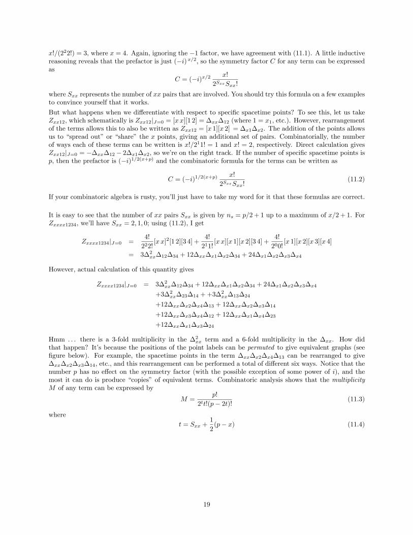
.x1 x2x3 x4
.
x1 x2
x3 x4
x4
.
x3
x1 x2
Symmetry Factor: 12Multiplicity: 6
Symmetry Factor: 3Multiplicity: 3
Symmetry Factor: 24Multiplicity: 1
-iλ
-iλ
-iλ
From (9.7) you can see that taking derivatives higher than 4 with respect to the interaction point requiresa new dummy integration variable (for example, to second order in � we�ll have Zxxxxyyyy). The aboveformulas for C and t then become
C = (�i)1=2(x+y+p) x! y!
2Sxx2SyySxx!Syy!Sxy!
t =1
2(p� x� y) + Sxx + Syy + Sxy
where Syy and Sxy are the exponents in �yy and �xy terms, respectively (the de�nition forM is unchanged).The extension of these expressions to higher orders of � should be obvious.
For n orders of interaction, the prefactor term will look like (�i)1=2(p+4n). However, since amplitudes arealways squared, the prefactor will square to unity, so most authors don�t even bother with it; consequently,I will dispense with it from here on.
It is important to note that the quantities x; y, etc. have 4 as their maximum value (that is, you must takefour di¤erentiations �per interaction�). Thus, for n-order problems the numerator in C will go like (4!)n.This explains the reason why we wrote the interaction term as V � �=4!; as the interaction exponentialis expanded, the 4! terms will cancel one another to all orders of �. In view of this, we can dispense withthese numerator factorials altogether and write the symmetry factors and multiplicities using the simple butrather ugly combinatorial expressions
C =
nYi;j=1(i�j)
1
2Sii Sij !and
M =p!
2tt!(p� 2t)! where
t =1
2(p� 4n) +
nXi;j=1(i�j)
Sij (11.5)
and where n is the order of interaction.
20

At the risk of being obsessively complete, I need to tell you that there is one more symmetry that can enterinto the above de�nition of C. Earlier, I noted that the symmetry factor is just a number that re�ects thenumber of ways that a diagram can be labelled (and by this I mean the interaction labels), so it is essentiallya combinatoric quantity. The expressions in (11.5) are the result of algebraic combinatorics, but there�sanother, purely topological, symmetry that resists being put into any formula (that is to say, I haven�t foundany). To see this, consider the following graph:
x1 x2
.
.
x y
a
b
..
This corresponds to n = 4; p = 2; Sxx = Syy = Saa = Sbb = 0; and all Sij = 1. According to (11.5), weshould then have
C =1
(20)4(1!)5= 1
However, the correct value is C = 1=2. Notice that the interaction indices a; b can be interchanged withoutchanging the signatures of any of the internal propagators. This interchangeability introduces an additionalfactor of two into the denominator of C. For really complicated diagrams, the topological symmetry factorcan be very di¢ cult to determine, and even seasoned quantum �eld theorists can get �ummoxed. In practice,you should use (11.5) �rst, then look to see if the graph has this type of exchange symmetry.
Lastly, please don�t confuse the symmetry operations that lie behind C and M with one another. Thesymmetry factor C always deals with permutations of the interaction labels, while M involves permutationsresulting from the relabelling of the external points p.
Let�s do a few examples to practice what (I hope) you�ve learned. The graph
x1 x2..x y
has n = 2, p = 2, Sxx = Syy = 0, Sxy = 3, t = 0 and M = 1. There�s no topological symmetry to worryabout, so
C =1
3!=1
6
One more, this time a bit more complicated to make sure you�ve got the hang of it:
...... .
.. .
x1
x2
x3
x4
ab
cd
e
f
gh
i
k
Here, n = 10, p = 4, Sbb = 1; Scd = 3; Ski = 2; Sih = 2; Shg = 2; Sgf = 2, with all other S terms equal tozero or 1; t = 0 and M = 1, and so
C =1
211!3!2!2!2!2!=
1
192
21

You will note from these examples that the only S terms you need to deal with come from internal lines(that is, lines that are connected from one interaction to another). With a little practice, you can �gure outC by just looking at the graphs.
As an exercise, let�s now calculate Z for the �rst-order, 4-point problem. To start, we expand (10.2) to �rstorder in �:
Z(�) =
h1� i�
4!
Rdx �4
�J(x)4
iZh
1� i�4!
Rdx �4
�J(x)4
iZ jJ=0
Using the notation we�ve developed, this is
Z(�) =Z � i�
4!
RZxxxx dx�
Z � i�4!
RZxxxx dx
�jJ=0
=Z � i�
4!
RZxxxx dx
1� i�4!
R(�3�2xx) dx
=Z � i�
4!
RZxxxx dx
1 + i�8
R�2xx dx
The 4-point Green�s function is then given by
G(x1; x2; x3; x4) = Z1234
=1
i4Z1234 � i�
24
RZxxxx1234 dx
1 + i�8
R�2xx dx
(11.6)
(The numerator will be evaluated at J = 0 after the di¤erentiations have been performed.) Using (11.5),we see that
Z1234jJ=0 = ��12�34 ��13�24 ��14�23while Z
Zxxxx1234 dxjJ=0 = 3�2xx�12�34 + 3�2xx�13�24 + 3�
2xx�14�23
+24
Z�x1�x2�x3�x4 dx
+12�xx
Z�x1�x2�34 dx+ 12�xx
Z�x2�x4�13 dx
+12�xx
Z�x2�x3�14 dx+ 12�xx
Z�x3�x4�12 dx
+12�xx
Z�x1�x4�23 dx+ 12�xx
Z�x1�x3�24 dx
Now, the denominator in (11.6) can be binomially inverted to �rst order in �, giving
1
1 + i�8
R�2xx dx
= 1� i�
8
Z�2xx dx
Multiplying this into the numerator in (11.6), we see that all of the double vacuum terms �2xx cancel eachother, and we�re left with
G(x1; x2; x3; x4) = ��12�34 ��13�24 ��14�23
�i�Z�x1�x2�x3�x4 dx
�12i�
��xx
Z�x1�x2�34 dx+ the 5 other terms
�(11.7)
22
The elimination of the pure vacuum term is a neat characteristic of normalization, and it can be shownto persist to all orders of the perturbation process. The �rst three terms in (11.7) do not participate in theinteraction and so can be ignored. Schematically, G represents the processes shown in the �gure on page 19.
Only the � term is fully �connected�in the sense that all propagators in the process are connected to oneanother. The point of connection is of course the interaction point x. Because of this, it is the only term inthe entire process that we�re really interested in; the other terms are all disconnected to some extent, as theyinclude propagators involving particles that go from one point to another without interacting with anything.Notice that the coe¢ cient of � is �i�. The vertex is the point x, but remember that this actually involvesintegration over all of spacetime,
R�x1�x2�x3�x4 dx.
Please note that we�ve focussed on a 4-point function for a good reason. It clearly represents a process inwhich two scalar particles are created at the lower end of � (points x1 and x2), propagate along until theyinteract with each other at some point x, then move away from each other until they are annihilated at theupper end of � at the points x3 and x4. If we look at the vertical and horizontal directions of these diagramsas representing time and space, respectively, then this is an ideal way of representing a scattering processfor two scalar particles (such as mesons).
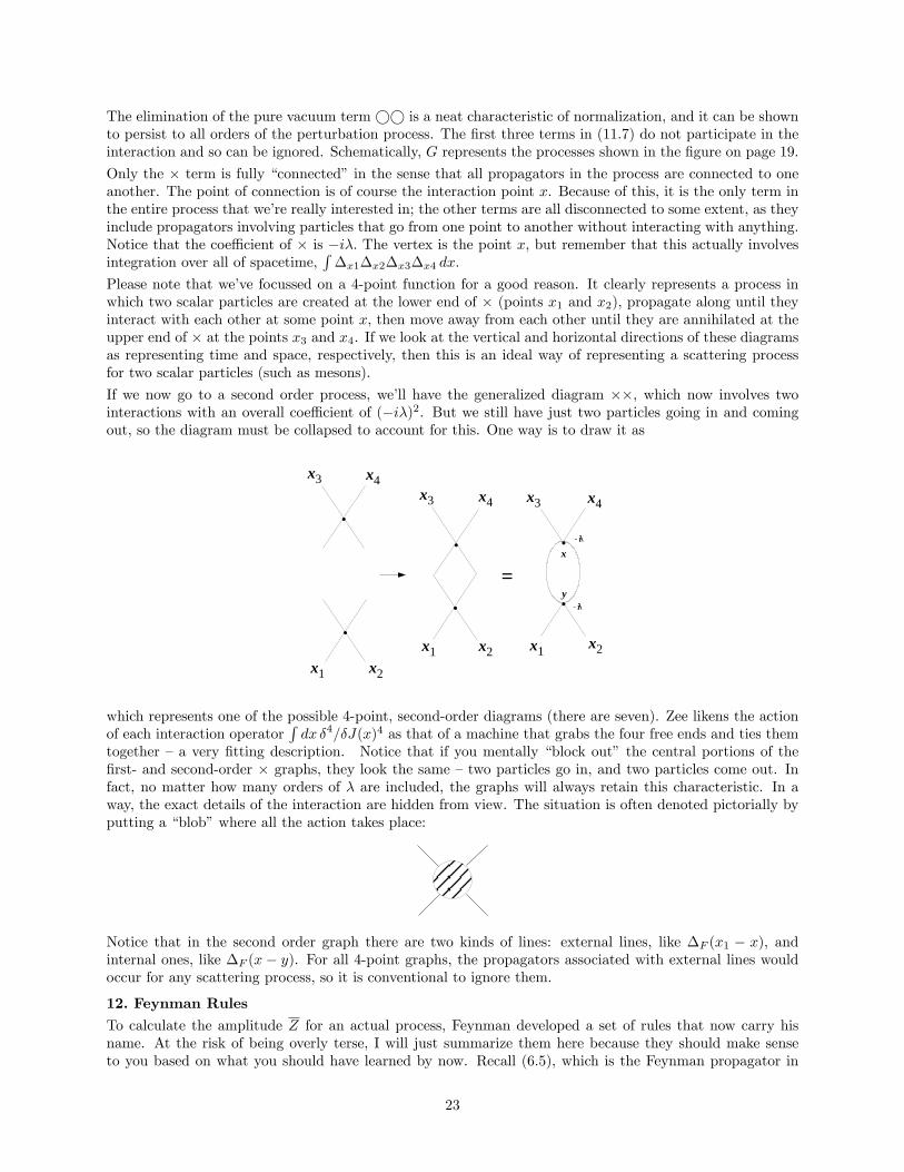
If we now go to a second order process, we�ll have the generalized diagram ��, which now involves twointeractions with an overall coe¢ cient of (�i�)2. But we still have just two particles going in and comingout, so the diagram must be collapsed to account for this. One way is to draw it as
x1 x2
.
.
=
x1 x2
x3 x4x3 x4
.
.
x
y
.
.
x3 x4
x1 x2
- iλ
- iλ
which represents one of the possible 4-point, second-order diagrams (there are seven). Zee likens the actionof each interaction operator
Rdx �4=�J(x)4 as that of a machine that grabs the four free ends and ties them
together �a very �tting description. Notice that if you mentally �block out� the central portions of the�rst- and second-order � graphs, they look the same �two particles go in, and two particles come out. Infact, no matter how many orders of � are included, the graphs will always retain this characteristic. In away, the exact details of the interaction are hidden from view. The situation is often denoted pictorially byputting a �blob�where all the action takes place:
Notice that in the second order graph there are two kinds of lines: external lines, like �F (x1 � x), andinternal ones, like �F (x � y). For all 4-point graphs, the propagators associated with external lines wouldoccur for any scattering process, so it is conventional to ignore them.
12. Feynman RulesTo calculate the amplitude Z for an actual process, Feynman developed a set of rules that now carry hisname. At the risk of being overly terse, I will just summarize them here because they should make senseto you based on what you should have learned by now. Recall (6.5), which is the Feynman propagator in
23
transform space. This is actually much more convenient than using the space form �xy, and we can use(6.5) to associate every line in a Feynman diagram with a four-momentum k. The Feynman rules for �4
QFT are then:
1. Draw all possible diagrams corresponding to the desired number of interactions and spacetime points,using time as the vertical axis and space as the horizontal axis. For each graph, label each internaland external line with a momentum kn and give it an arrow indicating direction (the direction can becompletely arbitrary). For each internal line, write the integral/propagator combinationZ
dkn(2�)4
i
k2n �m2
2. For each interaction vertex, write down a factor �i�.
3. For each interaction vertex, write a Dirac delta function that expresses the conservation of momentumabout that vertex:
(2�)4 �4
"Xi
ki
#where ki is positive if the line is entering the vertex and negative if it is exiting the vertex.
4. For each graph, there will be a residual delta function of the form (2�)4�4(k1+k2+ : : :) that expressesoverall conservation of momentum in the diagram. Cancel this term.
5. If there are any integrals remaining, you�ll have to do them. However, the delta functions you encoun-tered in Step 3 simplify things enormously, and you may not even have to do any integrals.
6. Calculate the symmetry factor for each graph using (11.5) and multiply this by the result obtained inStep 5.
7. Determine the total amplitude by taking the products of all the graphs. By convention, the totalamplitude is calledM.
That�s it. If any of the integrals diverge (as often happens for certain loop diagrams), then you�ll have toconsult a more advanced resource than this one �you�ve encountered the divergence problem (see the nextsection).
Note that for any physical process there can be a huge number of possible diagrams depending on how manyinteraction orders you�re willing to consider. As the interaction order n grows, the number and complexityof possible diagrams increases rapidly. However, the interaction term � is generally a small quantity; inquantum electrodynamics it is numerically equal to about 1/137), so the smallness of the (�i�)n term forlarge n e¤ectively reduces the probability that a complicated process will actually occur. This is why theperturbation approach works �you need only consider the most likely processes to get an accurate result.Even so, processes involving more than just a couple of orders in the interaction term can be a real pain tocalculate (Feynman used to joke that this is why we have graduate students). In the path-integral approachto the strong force (gluons), the interaction term � is relatively large, requiring the calculation of many termsto get decent convergence. The observed magnetic moment of the proton, for example, is approximately2.79275, but gluonic QFT gives us at best a �gure of 2.7, with a rather big margin of error. It seems nothingcomes easily in QFT!
Maybe some day a really bright young physicist will come along and discover a way to do the Z functionalintegral in closed form (if she does happen along, though, I hope she will turn her attention �rst to someof humankind�s more pressing problems, like the need for an environmentally friendly sustainable energysource).
ExamplesTo see how these rules work, let�s try two examples (for brevity, I�ll do this for speci�c graphs and not entireprocesses). For the � diagram, all the lines are external, so we don�t have to do very much. From (11.5),we have C = 1 and M = 1, and the amplitude is just Zxxxx1234 = �i�.
24

Now let�s calculate the amplitude for Zxxxxyyyy1234. We label it up as indicated below. We have twointeraction terms, which contribute an overall factor (�i�)2 to the amplitude. We have two internal lines,so we write
Z = (�i�)2Z Z
d4k
(2�)4d4q
(2�)4i
k2 �m2
i
q2 �m2(2�)4�4(k1 + k2 � k � q) (2�)4�4(k + q � k3 � k4)
This simpli�es to
Z = �2Z
d4k
(2�)41
(k2 �m2)
1
(k1 + k2 � k)2 �m2(2�)4�4(k1 + k2 � k3 � k4)
.
.
-iλ
-iλ
k1 k2
k3 k4
k q
x
y
x1 x2
x3 x4
where, as promised, there is a residual delta function expressing overall conservation of momentum. We cancelthis term and move on to the symmetry factor. For this diagram, Zxxxxyyyy1234 = [xx1][xx2][y x3][y x4][x y]2;therefore, Sxx = Syy = 0, Sxy = 2. Using (11.5), we have
C =1
2!=1
2
This leaves
Z =1
2�2Z
d4k
(2�)41
(k2 �m2)
1
(k1 + k2 � k)2 �m2
Does this integral converge? Well, for large momenta k the integral will go likeZd4k
k4=
Zk3dk
k4� log k �!1
Well, damn � the integral diverges. This is the famous �ultraviolet divergence� that bedeviled physicistsfor 20 years. Like I said, you�ll have to consult another resource if you want to �nd the amplitude for thisparticular second order process. (Zee gives the answer in Chapter 3 of his book. If you�re anything like me,you won�t be particularly happy with the solution approach, which is called renormalization).
13. Interpretation of Feynman�s Propagator for a Scalar ParticleIn the Feynman path integral, we have seen that the Feynman propagator �F (x�x0) plays a central role inthe perturbative expansion of the functional integral Z(J) in the presence of the interaction term ��4. Herewe�ll take a closer look at the propagator and provide an interpretation of its physical signi�cance. We have
�F (x� � x0�) =
Zd4k
(2�)4eik�(x
��x0�)
k2 �m2
25
where d4k = dk0 dkx dky dkz and k2 = g��k�k� = k20 � k2x � k2y � k2z = k20 ��!k 2(remember that we�re using
units in which c = �h = 1, while kx is the momentum in the x-direction, etc.). Thus, the propagator expressesthe probability amplitude that a particle of mass m will move from the spacetime point x0� to some otherpoint x�. Now let�s expand this in terms of the time variable k0:
�F (x� x0) =Zd3k ei
�!k ��!x
(2�)4
Zdk0 eik0x
0
k20 ��!k 2 �m2
If we now try to integrate this improper Fourier integral over dk0, we�re going to run into trouble becausethe pole occurs at k20 =
�!k 2 + m2, which inconveniently lies along the real axis of the complex plane. In
complex analysis, this is a disaster, because we cannot use the theory of residues to resolve the integral. Toget around this, we resort to the usual arti�ce of introducing a small imaginary term i� into the denominator:
�F (x� x0) =Zd3k ei
�!k ��!x
(2�)4
Zdk0 eik0x
0
k20 � !2 + i�(13.1)
where !2 =�!k 2 +m2 (I�ve always hated this trick, because in reality there�s no way to avoid the real axis,
but everybody does it, and it seems to work, so what the hell). We can then write
�F (x� x0) =Zd3k e�i
�!k ��!x
(2�)4
Zdk0 eik0x
0
(k0 � ! + i�)(k0 + ! � i�)(13.2)
I know what you�re thinking �the expanded denominator in (13.2) doesn�t match the one in (13.1). Butremember that the number i� is generic: if we multiply it by any positive real number, it�s still of order i�,so nothing has changed (sometimes it�s written as i� to show that i� has been multiplied by something).Anyway, we now have two complex poles, and evaluation of the integral is a snap. When x0 = ct is positive,we must use an integration contour in the upper complex plane; this surrounds only one pole (k0 = �!+ i�),and the residue is therefore 2�i exp[�i!x0]=(�2!) (I�ve let � = 0, so we can now pretend that we did nothingamiss when we stuck that i� term in). For x0 < 0 we have to close in the lower plane, where the pole isk0 = !� i�; this gives us the residue �2�i exp[+i!x0]=(2!). Putting this all together, we can now write thepropagator as
�F (x� x0) =�i(2�)3
Zd3k
2![e�i(!x
0+�!k ��!x )�(x0) + ei(!x
0��!k ��!x )�(�x0)]
where �(�x0) is the unit step function for forward or backward time, which is either zero or one dependingon the sign of its argument. To make the terms in
�!k � �!x symmetric, notice that we can replace k with �k
in the integral without changing anything :
d3k = k2dk sin �k d�k d�k = d3(�k)
So we then have, equivalently,
�F (x� x0) =�i(2�)3
Zd3k
2![e�i(!x
0��!k ��!x )�(x0) + ei(!x0��!k ��!x )�(�x0)] (13.3)
Notice that ! has units of energy; that is, if we put back the speed of light term c in !2 =�!k 2 +m2, we
recover the familiar relativistic energy relation E2 = c2�!p 2 +m2c4, where E = �h!. You may recall fromelementary quantum mechanics that a wave corresponding to a particle having positive energy propagateslike � exp[�iEt=�h]. We can see this quantity in (13.3), where it is constrained to move in the forwardtime direction by �(x0). This is a good thing �we interpret this as positive-energy particles moving forwardin time in the Feynman propagator. However, there is that other term exp[iEt=�h] �(�x0) in (13.3) which,by the same logic, must be interpreted as negative-energy particles propagating backward in time. How dowe make sense of this? Simple �if E is negative and t is running backward, the conjugate pair Et can alsobe viewed as positive E and positive t. We therefore have a prescription for positive-energy antiparticlesmoving forward in time, since both views are mathematically equivalent. The ability of the propagator to
26

accommodate scalar (bosonic) antiparticles into the same theory is just one of the fantastic successes thatFeynman�s calculus has achieved. This same prescription holds when we go from a scalar theory to a spin1/2 fermionic theory, which can also be developed using the same basic path integral approach.Incidentally, sooner or later you�re going to have to evaluate 4-dimensional integrals �all the way,�not justthrough dx0. When you do, you may initially have trouble (like I did) dealing with the notation �d4k.�
Since many integrands will have terms like ei�!k ��!x = eikx cos �, it makes sense to consider doing the integrals
in spherical coordinates, where d3k = k2dk sin � d� d� (just think of the momentum 3-vector�!k as behaving
like the radial vector �!r ). In four dimensions, we have k2 = k20 � k2x � k2y � k2z = k20 ��!k 2, so you�ll have to
mind the occasional confusion between k2 (which is 4-dimensional), and�!k 2, which is also usually denoted
as k2 as well.There�s yet another way of looking at d4k. Consider a 90
�rotation of the time coordinate in the complex
plane so that t �! it. Then k2 = �k20 � k2x � k2y � k2z , and we say that space is �euclidean.�In this space,any direction is mathematically the same as any other, so that d4k = k3dk (that is, it depends only on themagnitude of the four-vector k). Why k3 and not k2? In regular polar coordinates, one has dA = r dr d�and dV = r2dr sin � d� d�, so the exponent on r is always one less than number of dimensions. In tensorlanguage, we have dA =
pg dx1dx2 and dV =
pg dx1dx2dx3, where
pg is the metric determinant (exactly
how the tensor prescription produces d4k = k3dk in four dimensions escapes me for the moment).As you�ve already seen, you�re going to encounter Feynman diagrams (loop diagrams, in particular) that givedivergent results. This complication (sometimes called the �problem of the in�nities�) plagued quantum �eldtheory until the rather dubious (in my opinion) mathematical technique known as renormalization arrivedon the scene to bail out the theory. I�m certainly not going to discuss renormalization in any detail in thissimple write-up, but I can give you a taste of what the approach involves.Consider the 2-point function to �rst order in �, which is
G(x1; x2) = Z12 =1
i2Z12 � i�
24
RZxxxx12 dx
1 + i�8
R�2xx dx
= i�12 �1
2��xx
Z�x1�x2 dx
Expanding the integral term, we have
( ) = �12��xx
Zdp dq dx
(2�)8eipxe�ipx1eiqxe�iqx2
(p2 �m2)(q2 �m2)
= �12��xx
Zdp dq �4(p+ q)
(2�)4e�ipx1e�iqx2
(p2 �m2)(q2 �m2)
= �12��xx
Zdp
(2�)4eip(x1�x2)
(p2 �m2)2
Now, since
i�12 = i
Zdp
(2�)4eip(x1�x2)
(p2 �m2)
we have
G(x1; x2) = i
Zdp eip(x1�x2)
(2�)4(p2 �m2)
�1 +
i��xx2(p2 �m2)
�Binomial expansion allows us to write
1 +i��xx
2(p2 �m2)=
�1� i��xx
2(p2 �m2)
��1so that
G(x1; x2) = i
Zdp eip(x1�x2)
(2�)4(p2 � em2)
= ie�12 = eG(x1; x2)27

where em2 = m2 + i��xx=2. Thus, we have a new version of the 2-point function, eG(x1; x2), that looksjust like G(x1; x2) except that it contains the revised mass term em. Since �xx diverges, em is an in�nitequantity � the e¤ect of the interaction term is to make the particle mass in�nite! This is annoying, butin the laboratory we always measure the physical mass m, which is not necessarily the same quantity thatstarts out in the Lagrangian (at least when the interaction term is present). The mass is then said to berenormalized.
Along the same line, you may have noticed that the denominator in the Feynman propagator, k2 �m2, isnormally zero (it�s just the relativistic mass-energy relation E2 � c2p2 � m2c4 = 0). But in QFT, whenk2�m2 6= 0 we say that the particle is o¤ mass shell, so the integral doesn�t blow up. Particle 4-momentumconservation has to hold at each interaction vertex, but not when the particle is just �propagating along.�
If you can swallow all of this, I congratulate you!
14. Is Quantum Field Theory Real?Let�s wrap up this overly long discussion by asking the question �Is there any reason to believe that quantum�eld theory is not an accurate depiction of reality after all? In spite of its impressive ability to correctlypredict a wide variety of experimental results, we cannot rigorously prove that all those in�nite-dimensionalintegrals are convergent. To see this, let�s take an exceedingly simple problem: a single Gaussian integralwith an interaction term but no kinetic term:
Z(m;�) =
Ze�
12m
2�2���4d� (14.1)
where � is the coupling constant. You can think of this as a vastly simpli�ed version of what we�re trying todo with QFT. Certainly, (14.1) must have a solution if QFT is to have any chance of being a valid theory!Although this integral cannot be evaluated in closed form, we can do it term by term by expanding theexponential in ��4. We then have
Z(m;�) =1Xn=0
(�1)n�n
n!
Z�4n e�
12m
2�2d�
The integral can be performed by noticing that repeated di¤erentiation of the Gaussian integral
Z(m; 0) =
Ze�
12m
2�2d� =p2�m�1
with respect to m will introduce enough �2 terms into the integral for us to build up the required �4n term(this is just like using the source term J(x) in the functional integral to �bring down�the expansion termsassociated with ��4 in the full theory). The answer is
Z(m;�) =
p2�
m+
p2�
m
1Xn=1
(�1)n�n(4n� 1)!!n!m4n
The double factorial can be written as
(4n� 1)!! = 2(4n� 1)!4n(2n� 1)!
so that
Z(m;�) =
p2�
m+
p2�
m
1Xn=1
(�1)n 2�n(4n� 1)!n!4nm4n(2n� 1)!
Does this quantity converge? For large factorials, we can use Sterling�s approximation N ! �p2�N [N=e]N
to simplify things. Plugging this into the above, I get
Z(m;�) ���16�nm4e
�n
28

Well, this is a disaster � as n approaches in�nity, the integral Z blows up. This is quite discouraging,particularly in view of the fact that (14.1) is the simplest possible integral we can imagine that is QFTish.Can we ever hope that the in�nite-dimensional integrals in interacting quantum �eld theory have anythingto do with reality?In my opinion, there are few satisfactory ways out of this dilemma. It is known in QFT that renormalizationforces us to abandon the idea that the actual values for mass and charge are really what we think theyare. The renormalized mass of a particle, as you have seen, is in�nite. Is it possible that an in�nite masssomehow cancels the in�nity in Z(m;�) for large values of n? Very unlikely, because the actual value for thecoupling constant � isn�t what we think it is, either! Most physicists believe that QFT is valid only within acertain range of n which they call the radius of convergence. Within this range, QFT provides the fantasticaccuracy it has shown for quantum electrodynamics and other applications, while outside this range it givesnonsensical in�nities.As little more than a neophyte myself, I would like to o¤er another possible answer, and that is this: Muchof the mathematics that physicists use is non-rigorous (it may look impressive at �rst glance, but it is oftenvery sloppy and makes mathematicians cringe), and it�s possible that we�ve just pushed things further thanwe should have in order to obtain a solution. In my opinion, physicists are not above resorting to dirtytricks to make things work, especially when improper integrals are lurking about. A case in point is theintegral expression for Z(J; �) in (9.1). I won�t go into it, but physicists usually insert the term 1
2 i��2 into
the Lagrangian (where � is a small, positive real constant) which ensures that the integral will converge;afterwards, they set � = 0, and nobody is any the wiser. They can even rotate the spacetime coordinates tomake time imaginary, which also makes the Z integral converge. I�ll give you an example that may be easierto understand. Consider the much simpler quantity
I(!) =
1Z0
ei!x dx
which occurs occasionally in quantum mechanical problems (! is taken to be real and positive). Thisintegrates straightforwardly to
I(!) =1
i!
�ei!1 � 1
�At x =1, the exponential oscillates violently, so I(!) doesn�t converge. However, if we replace ! with !+ i�in the integrand, this becomes
I(!) =1
i(! + i�)
�ei!xe��1 � 1
�The e��1 term now kills o¤ the o¤ending harmonic factor, giving us I(!) = i=! after we cancel the remaining� in the denominator. As an engineer, this kind of mathematical chicanery has always bothered me, but Iguess it beats not having a solution.
15. Final Thoughts
1. You should look at all this as a very elementary beginning to QFT. In the end, it�s not all that interestingbecause what we�ve been discussing is scalar QFT; much more interesting is fermionic QFT, especiallyquantum electrodynamics. It is here that you will �nd the kind of Feynman diagrams you�ve no doubtseen in books, with the squiggly photon lines and such, along with some pretty amazing calculations.But the scalar version is a good place to get your feet wet.
2. Anthony Zee has written a wonderful book (see references) in which he has tried to encapsulate thegist of QFT �in a nutshell.�He bemoans the fact that what started out as an introductory overviewended up covering over 500 pages. Now I know how he feels, because it is impossible to cover this topicin a few dozen pages or so. I strongly encourage you to get his book and look at how rich QFT is, evenat a very elementary level.
3. Remember that the square of the amplitudeM is proportional to the probability that the process ina particular Feynman diagram will occur. The proportionality constant comes from what is known asFermi�s Golden Rule (this is a simple formula, but I will not go into it any further here). Putting allthis together, you can accurately calculate things like particle decay rates and event cross sections.
29

4. The Feynman rules for quantum electrodynamics (QED) are the same as those for scalar particles, butthe terms are a little di¤erent. For example, the photon propagator is proportional to i=k2, which mightbe expected since the photon is massless. While the divergence problem persists in QED, physicistshave developed powerful renormalization techniques which, while perhaps aesthetically unpleasing,have resulted in calculations whose predictive accuracy is nothing less than fantastic (the calculatedgyromagnetic ratio of the electron, for example, matches the experimental value to within 10 decimalplaces).
5. Lastly, think of how amazing all this is �in spite of our pathetic model-building and mathematical hand-waving over particles and things that we can never actually observe (or truly understand), quantum�eld theory is nothing less than a glimpse into the mind of God. Although the path integral is abeautiful mathematical edi�ce, imagine how incredibly beautiful the true reality behind the curtain ofexistence must be!
And with that rather philosophical remark, I bid you adieu and God bless.
References
1. P.A.M. Dirac, The Principles of Quantum Mechanics. Clarendon Press, 4th ed., Oxford, 1967. Diracis just about my favorite physicist, perhaps in part because he started out in life as an electricalengineer! Born in Bristol, England on 8 August 1902 to a Swiss father and English mother, Dirac wasalready a giant in the �eld of quantum theory by the time he was 25. Aloof (but not unfriendly) andultra-taciturn (look up taciturn in the dictionary and you�ll �nd his picture), Dirac preferred solitarywalks and thinking about physics to just about everything else. He discovered the relativistic electronequation in 1927 �to me, the most profound and beautiful achievement of the human mind.
A brilliant physicist, Dirac was an equally brilliant mathematician. The Dirac delta function is anindispensible tool to physicists and mathematicians alike, while his introduction of creation and an-nihilation operators has made the harmonic oscillator problem transparent to generations of physicsstudents. Dirac�s mind also gave us antimatter, the graviton, the magnetic monopole, quantum elec-trodynamics, and the four-component spinor formalism. He is said to have been particularly happywith his development of the bra and ket �language� of modern quantum mechanics, which is morecommonly (and rightly) called Dirac notation.
Elected Lucasian Professor of Mathematics at St. John�s College in Cambridge in 1932 (Isaac Newton�sold post), Dirac won the Nobel Prize in physics in 1933, sharing it with Erwin Schrödinger. In 1937,Dirac married the sister of fellow physics Nobel laureate Eugene Wigner. In 1969, Dirac left Cambridgeand in 1972 joined the faculty of Florida State University in Tallahassee! Dirac died there on 20 October1984 and was buried at Roselawn Cemetery, not far from the school. In November 1995, a plaque wasplaced in his honor at Westminster Abbey in London, close to the tomb of Newton (Stephen Hawking,the current Lucasian Professor, delivered the dedication address via voice synthesizer). On the plaqueis engraved �i � @ = m,�Dirac�s relativistic electron equation. In a saner and more orderly world,Dirac�s name would be as recognizable as Einstein�s or Newton�s. The fact that it is not is a greatmystery to the world�s physicists and mathematicians, who owe so much to this quiet genius fromBristol.
Dirac�s book on quantum mechanics appeared in 1930 and became an instant classic (Dirac�s pathintegral �analogy�remark appears in this book). However, I have had one hell of a time understandingit, and I simply don�t know why � maybe it�s the language Dirac uses, or maybe it�s the book�stypesetting; it just doesn�t speak to me. Maybe you�ll have better luck.
2. D. Gri¢ ths, Introduction to Elementary Particles. Wiley & Sons, New York, 1987. In my opinion, thebest book of its kind �cleverly written and lucid, with much of Gri¢ ths�wonderful humor thrown into liven things up. I highly recommend it.
30

3. F. Halzen and A. Martin, Quarks and Leptons: An Introductory Course in Modern Particle Physics.Wiley & Sons, New York, 1984. Kind of like a companion book to Gri¢ ths� text. A recommendedintroduction.
4. M. Kaku, Quantum Field Theory: A Modern Introduction. Oxford University Press, New York, 1993.Highly readable for the beginner by an author who is also an expert on superstring theory. The bookincludes a chapter on this topic, along with supergravity.
5. P. Ramond, Field Theory : A Modern Primer. Addison-Wesley, 2nd ed., Redwood City, California,1989. Written by one of the giants of string theory, this book is somewhat more advanced and detailedthan Kaku�s text but is very readable nevertheless. I was disappointed to �nd that some of the formulasI thought I had discovered were in this book! Also highly recommended.
6. L. Ryder, Quantum Field Theory. Cambridge University Press, 2nd ed., Cambridge, 1996. The mostcomprehensive and readable book on the subject that I have seen to date. Alas, this second editionincludes a chapter on supersymmetry, and is far over my head.
7. J.J. Sakurai, Modern Quantum Mechanics. Addison-Wesley, Redwood City, California, 1985. Trag-ically, Sakurai died in an accident at the age of 49, and this book was �nished by a colleague. Thechapters written by Sakurai include the most lucid expositions on quantum physics I have ever read,and I cannot recommend it too highly.
8. J.J. Sakurai, Advanced Quantum Mechanics. Addison-Wesley, Redwood City, California, 1967. Oddlyenough, Sakurai wrote this book many years before the previously-cited text. In the preface, he writesthat the purpose of the book was to present QFT �in a manner that cannot be made any simpler.�Well, I can�t make head or tails out of this book, and if you�re just starting out, I suggest you stayaway from it.
9. J. Schwinger (ed.), Selected Papers on Quantum Electrodynamics. Dover Publications, 1958. Hereyou�ll �nd the collected works of many great physicists on QED, including Dirac�s 1933 paper on thequantum mechanical action principle and Feynman�s 1948 classic on the path integral.
10. R. Shankar, Principles of Quantum Mechanics. Yale University, 2nd ed., New York, 1994. Thistextbook is an undergraduate favorite, and includes two chapters on the path integral and applications.If your basic quantum mechanics is a little rusty, this is a great book to seek out.
11. A. Zee, Quantum Field Theory in a Nutshell. Princeton University Press, Princeton, New Jersey, 2003.Years ago I wondered why nobody had ever written a book along the lines of �Quantum Field Theoryfor Dummies.�Well, Dr. Zee has done it, and done it well. Even if your math is not quite up to QFTstandards, you will bene�t from his insightful, comprehensive, enthusiastic and very understandableapproach to the subject. The book includes relatively easy mathematical treatments of many relatedtopics, including renormalization, quantum gravity and cosmology, symmetry breaking, condensedmatter theory, grand uni�cation and strings. This is the book I wish I had 25 years ago. If you buyjust one book on QFT, get this one.
31