field evaluation of compaction monitoring technology: phase i

FIELD EVALUATION OF COMPACTION MONITORING

TECHNOLOGY: PHASE I

Sponsored bythe Iowa Department of Transportationand the Iowa Highway Research Board

Final Report September 2004

Iowa DOT Project TR-495CTRE Project 03-141

Partnership for Geotechnical Advancement

The opinions, findings, and conclusions expressed in this publication are those of the authors andnot necessarily those of the Iowa Department of Transportation or the Iowa Highway Research Board.

CTRE’s mission is to develop and implement innovative methods, materials, and technologies forimproving transportation efficiency, safety, and reliability while improving the learning environment ofstudents, faculty, and staff in transportation-related fields.

Technical Report Documentation Page

1. Report No. 2. Government Accession No. 3. Recipient’s Catalog No. Iowa DOT Project TR-495

4. Title and Subtitle 5. Report Date September 2004 6. Performing Organization Code

Field Evaluation of Compaction Monitoring Technology: Phase I

7. Author(s) 8. Performing Organization Report No. David J. White, Edward J. Jaselskis, Vernon R. Schaefer, E. Thomas Cackler, Isaac Drew, and Lifeng Li

CTRE Project 03-141

9. Performing Organization Name and Address 10. Work Unit No. (TRAIS) 11. Contract or Grant No.

Center for Transportation Research and Education Iowa State University 2901 South Loop Drive, Suite 3100 Ames, IA 50010-8634

12. Sponsoring Organization Name and Address 13. Type of Report and Period Covered Final Report 14. Sponsoring Agency Code

Iowa Department of Transportation 800 Lincoln Way Ames, IA 50010 15. Supplementary Notes 16. Abstract This Phase I report describes a preliminary evaluation of a new compaction monitoring system developed by Caterpillar, Inc. (CAT), for use as a quality control and quality assurance (QC/QA) tool during earthwork construction operations. The CAT compaction monitoring system consists of an instrumented roller with sensors to monitor machine power output in response to changes in soil-machine interaction and is fitted with a global positioning system (GPS) to monitor roller location in real time. Three pilot tests were conducted using CAT’s compaction monitoring technology. Two of the sites were located in Peoria, Illinois, at the Caterpillar facilities. The third project was an actual earthwork grading project in West Des Moines, Iowa. Typical construction operations for all tests included the following steps: (1) aerate/till existing soil; (2) moisture condition soil with water truck (if too dry); (3) remix; (4) blade to level surface; and (5) compact soil using the CAT CP-533E roller instrumented with the compaction monitoring sensors and display screen. Test strips varied in loose lift thickness, water content, and length. The results of the study show that it is possible to evaluate soil compaction with relatively good accuracy using machine energy as an indicator, with the advantage of 100% coverage with results in real time. Additional field trials are necessary, however, to expand the range of correlations to other soil types, different roller configurations, roller speeds, lift thicknesses, and water contents. Further, with increased use of this technology, new QC/QA guidelines will need to be developed with a framework in statistical analysis. Results from Phase I revealed that the CAT compaction monitoring method has a high level of promise for use as a QC/QA tool but that additional testing is necessary in order to prove its validity under a wide range of field conditions. The Phase II work plan involves establishing a Technical Advisor Committee, developing a better understanding of the algorithms used, performing further testing in a controlled environment, testing on project sites in the Midwest, and developing QC/QA procedures.

17. Key Words 18. Distribution Statement compaction monitoring—earthwork construction—machine energy—quality control/quality assurance—soil compaction

No restrictions.

19. Security Classification (of this report)

20. Security Classification (of this page)

21. No. of Pages 22. Price

Unclassified. Unclassified. 188 NA

FIELD EVALUATION OF COMPACTION MONITORING TECHNOLOGY: PHASE I

Iowa DOT Project TR-495

CTRE Project 03-141

Principal Investigator E. Thomas Cackler, Director

Partnership for Geotechnical Advancement, Iowa State University

Co-Principal Investigators David J. White, Assistant Professor

Department of Civil, Construction and Environmental Engineering, Iowa State University

Edward J. Jaselskis, Associate Professor Department of Civil, Construction and Environmental Engineering, Iowa State University

Vernon R. Schaefer, Professor

Department of Civil, Construction and Environmental Engineering, Iowa State University

Research Assistants Isaac Drew Lifeng Li

Authors

David J. White, Edward J. Jaselskis, Vernon R. Schaefer, E. Thomas Cackler, Isaac Drew, and Lifeng Li

Preparation of this report was financed in part

through funds provided by the Iowa Department of Transportation through its research management agreement with the Center for Transportation Research and Education.

Center for Transportation Research and Education

Iowa State University 2901 South Loop Drive, Suite 3100

Ames, IA 50010-8634 Phone: 515-294-8103 Fax: 515-294-0467

www.ctre.iastate.edu

Final Report • September 2004

iii

TABLE OF CONTENTS

EXECUTIVE SUMMARY ........................................................................................................XIII

INTRODUCTION ...........................................................................................................................1 Project Scope .......................................................................................................................2 Research Objectives.............................................................................................................3 Significant Findings and Recommendations from Phase I ..................................................3

BACKGROUND .............................................................................................................................5 Soil Compaction...................................................................................................................5

Soil Type..................................................................................................................6 Moisture Content .....................................................................................................7 Compaction Effort ...................................................................................................8

Quality Control of Field Compaction ..................................................................................9 Intelligent Compaction ..........................................................................................10 Continuous Compaction Control ...........................................................................11 Future Applications of Compaction Technologies ................................................11

Theoretical Development...................................................................................................12

RESEARCH METHODOLOGY...................................................................................................14 Description of Pilot Tests ..................................................................................................14

Project No. 1 – Caterpillar Peoria Proving Ground (PPG) Field Test...................14 Project No. 2 – Caterpillar Edwards Facility Field Test........................................15 Project No. 3 – Wells Fargo Headquarter Project, Des Moines, IA ......................15

In situ Test Measurements .................................................................................................16 Analysis of Compaction Monitoring Output .....................................................................16

PILOT PROJECTS RESULTS AND DISCUSSION....................................................................18 Project No. 1 – Caterpillar Peoria Proving Ground (PPG) Field Test...............................18

Soil Index Properties..............................................................................................18 Soil Strength and Stiffness.....................................................................................21 Site Preparation and Construction Operations.......................................................23 In situ Test Measurements .....................................................................................24 Compaction Monitoring Output Results................................................................26 Regression Analysis...............................................................................................30 Key Findings and Recommendations – Project No. 1. ..........................................34

Project No. 2 – Caterpillar Edwards Facility Field Test....................................................35 Soil Index Properties..............................................................................................35 Soil Strength and Stiffness.....................................................................................38 Site Preparation and Compaction Operations........................................................40 In situ Test Measurements .....................................................................................41

iv

Compaction Monitoring Output Results................................................................52 Exploratory Study of Compaction Monitoring Output..........................................57 Variability of Power Values ..................................................................................59 Regression Analysis...............................................................................................62 Key Findings and Recommendations – Project No. 2. ..........................................64

Project No. 3 – Wells Fargo Headquarter Project, Des Moines, IA ..................................66 Soil Index Properties..............................................................................................66 Site Preparation and Compaction Operations........................................................67 In situ Test Measurements .....................................................................................70 Compaction Monitoring Output Results................................................................79 Exploratory Study of Compaction Monitoring Output..........................................84 Regression Analysis...............................................................................................86 Key Findings and Recommendations – Project No. 3 ...........................................88

SUMMARY AND CONCLUSIONS ............................................................................................90

RECOMMENDATIONS...............................................................................................................91 Develop Better Understanding of Algorithms ...................................................................91 Perform Controlled Experiments .......................................................................................91 Field Testing ......................................................................................................................92 Develop QC/QA Guidelines ..............................................................................................92 Investigate Transferability to Asphalt Pavement...............................................................93

REFERENCES ..............................................................................................................................94

APPENDIX A: LABORATORY TEST RESULTS – PROJECT NO. 1 ......................................96

APPENDIX B: STATISTICAL ANALYSIS RESULTS– PROJECT NO. 1 .............................102

APPENDIX C: LABORATORY AND FIELD TEST RESULTS – PROJECT NO. 2 ..............110

APPENDIX D: STATISTICAL ANALYSIS RESULTS – PROJECT NO. 2............................152

APPENDIX E: LABORATORY AND FIELD TEST RESULTS – PROJECT NO. 3...............168

APPENDIX F: STATISTICAL ANALYSIS RESULTS – PROJECT NO. 3 ............................173

v

LIST OF FIGURES

Figure 1. CAT Compaction monitoring system components ..........................................................2 Figure 2. Standard and Modified compaction curves (Holtz and Kovacs 1981).............................6 Figure 3. Effect of soil type on dry unit weight versus water content (Spangler and Handy 1982)7 Figure 4. Simplified 2-D free body diagram of stresses acting on a rigid compaction drum........13 Figure 5. Laboratory compaction test results on PPG till for various compaction energies .........18 Figure 6. Semi-logarithmic relationship between compaction energy and optimum water content

and maximum dry unit weight (PPG till)...........................................................................19 Figure 7. Influence of compaction energy on dry unit weight as a function of moisture content

(PPG till) ............................................................................................................................20 Figure 8. Energy as a function of moisture content for various degrees of compaction (PPG till)20 Figure 9. Semi-logarithmic relationship between undrained shear strength and compaction

energy as a function of water content (PPG till)................................................................22 Figure 10. Semi-logarithmic relationship between secant modulus and compaction energy as a

function of water content (PPG till)...................................................................................22 Figure 11. Compaction being performed by CAT CP-533E roller in reverse direction for test

strip 2A ..............................................................................................................................24 Figure 12. Trimble GPS base-station system used in situ test point locations ..............................25 Figure 13. CIV stiffness measurements using the Clegg impact hammer.....................................25 Figure 14. GeoGauge stiffness measurements...............................................................................26 Figure 15. DCP strength profile measurements.............................................................................26 Figure 16. Compaction monitor results for test strips 2 and 3.......................................................27 Figure 17. Coverage monitor results for test strips 2 and 3...........................................................28 Figure 18. Machine power values as a function of roller pass for test strip 2A at Peoria Proving

Grounds..............................................................................................................................28 Figure 19. Machine power values as a function of roller pass for test strip 2B at Peoria Proving

Grounds..............................................................................................................................29 Figure 20. Machine power values as a function of roller pass for test strip 3A at Peoria Proving

Grounds..............................................................................................................................29 Figure 21. Machine power values as a function of roller pass for test strip 3B at Peoria Proving

Grounds..............................................................................................................................30 Figure 22. R2 versus moving average span for models predicting dry density .............................33 Figure 23. R2 versus moving average span for models predicting CIV ........................................33 Figure 24. Laboratory compaction test results on Edwards till for various compaction energies.35 Figure 25. Semi-logarithmic relationship between compaction energy, optimum water content,

and maximum dry unit weight (Edwards till) ....................................................................36 Figure 26. Influence of compaction energy on dry unit weight as a function of moisture content

(Edwards till) .....................................................................................................................37 Figure 27. Energy as a function of moisture content for various degrees of compaction (Edwards

till)......................................................................................................................................38 Figure 28. Semi-logarithmic relationship between undrained shear strength and compaction

energy as a function of water content (Edwards till) .........................................................39 Figure 29. Semi-logarithmic relationship between secant modulus and compaction energy as a

function of water content (Edwards till) ............................................................................39 Figure 30. Comparison of drive core and nuclear density values..................................................42 Figure 31. Depth versus density results for nuclear gauge (Test Strip C) .....................................42

vi

Figure 32. Test strips F and G after tilling with RR350 ................................................................43 Figure 33. Test strips A through D after compaction ....................................................................43 Figure 34. Surface condition after compaction for Test Strip B....................................................44 Figure 35. Surface condition after compaction for Test Strip C....................................................44 Figure 36. Surface condition after compaction for Test Strip D ...................................................44 Figure 37. Surface condition after compaction for Test Strip E....................................................45 Figure 38. Surface condition after compaction for Test Strip F ....................................................45 Figure 39. Surface condition after compaction for Test Strip G ...................................................45 Figure 40. TDR equipment ............................................................................................................47 Figure 41. TDR vs. nuclear and oven volumetric water contents (%)...........................................47 Figure 42. TDR standard output vs. calibrated moisture content based on nuclear gauge m% ....48 Figure 43. TDR m% vs. actual m% based on actual m%..............................................................48 Figure 44. Nuclear versus oven on volumetric basis .....................................................................49 Figure 45. Average MDCP index vs. moisture..............................................................................50 Figure 46. Average MDCP index vs. lift thickness .......................................................................51 Figure 47. CBR plot of test point 4 from test strip F .....................................................................51 Figure 48. Influence of water content on CIV measurements .......................................................52 Figure 49. Monitor output for machine energy after 1, 4, and 10 roller passes (a – c) on test strip

H at Edwards Test Facility.................................................................................................53 Figure 50. Monitor output for machine coverage after 1, 4, and 10 roller passes (a – c) on test

strip H at Edwards Test Facility ........................................................................................54 Figure 51. Machine power values as a function of roller pass for test strip G at Edwards Test

Facility ...............................................................................................................................55 Figure 52. Machine power values as a function of roller pass for test strip H at Edwards Test

Facility ...............................................................................................................................56 Figure 53. Machine power values as a function of roller pass for test strip D at Edwards Test

Facility ...............................................................................................................................56 Figure 54. Machine power values as a function of roller pass for test strip F at Edwards Test

Facility ...............................................................................................................................57 Figure 55. Box plots for gross power versus number of passes for test strip A ............................58 Figure 56. Box plots for net power versus number of passes for test strip A................................58 Figure 57. Histogram for standard deviation for net power ..........................................................60 Figure 58. Histogram for standard deviations for gross power .....................................................60 Figure 59. Histogram of COV values for gross power ..................................................................61 Figure 60. Histogram of COV values for net power......................................................................61 Figure 61. Laboratory compaction test results on Des Moines clay 1 (natural on-site soil) for

standard Proctor energy .....................................................................................................66 Figure 62. Laboratory compaction test results on Des Moines clay 2 (fill material) for standard

Proctor energy....................................................................................................................67 Figure 63. Machine energy output and resulting dry unit weight as a function of roller passes on

test strip A..........................................................................................................................71 Figure 64. Machine energy output and resulting percent standard Proctor as a function of roller

passes on test strip A..........................................................................................................71 Figure 65. Machine energy output and resulting MDCP as a function of roller passes on test strip

A.........................................................................................................................................72 Figure 66. Machine energy output and resulting CIV as a function of roller passes on test strip A72 Figure 67. Machine energy output and resulting dry unit weight as a function of roller passes on

test strip B ..........................................................................................................................73

vii

Figure 68. Machine energy output and resulting percent standard Proctor as a function of roller passes on test strip B..........................................................................................................73

Figure 69. Machine energy output and resulting MDCP as a function of roller passes on test strip B.........................................................................................................................................74

Figure 70. Machine energy output and resulting CIV as a function of roller passes on test strip B74 Figure 71. Machine energy output and resulting dry unit weight as a function of roller passes on

test strip C (no vibratory)...................................................................................................75 Figure 72. Machine energy output and resulting percent standard Proctor as a function of roller

passes on test strip C (no vibratory)...................................................................................75 Figure 73. Machine energy output and resulting MDCP as a function of roller passes on test strip

C (no vibratory) .................................................................................................................76 Figure 74. Machine energy output and resulting CIV as a function of roller passes on test strip C

(no vibratory) .....................................................................................................................76 Figure 75. Machine energy output and resulting dry unit weight as a function of roller passes on

test strip CV (vibratory).....................................................................................................77 Figure 76. Machine energy output and resulting percent standard Proctor as a function of roller

passes on test strip CV (vibratory).....................................................................................77 Figure 77. Machine energy output and resulting MDCP as a function of roller passes on test strip

CV (vibratory)....................................................................................................................78 Figure 78. Machine energy output and resulting CIV as a function of roller passes on test strip

CV (vibratory)....................................................................................................................78 Figure 79. Compaction machine ....................................................................................................79 Figure 80. Monitor output for machine energy after 1-8 roller passes (a – h) on test strip B at W.

Des Moines project site......................................................................................................82 Figure 81. Monitor output for machine coverage after 1-4 roller passes (a – d) on test strip A at

W. Des Moines project site................................................................................................83 Figure 82. Box plots for engine powers on level test strips...........................................................84 Figure 83. Box plots for engine powers when driving up and down slope, alternately ................85 Figure 84. Box plots of measured soil properties for third field test .............................................86 Figure 85. Suggested test point settings to improve R2 .................................................................88 Figure A1. Dry unit weight results from unconfined compression tests for various compaction

energies (Edwards till) .......................................................................................................97 Figure A2. Unconfined compression results for various compaction energies at approximately

5.0% moisture content (PPG till) .......................................................................................98 Figure A3. Unconfined compression results for various compaction energies at approximately



10.0% moisture content (PPG till) .....................................................................................99 Figure A6. Unconfined compression results delivered with a compaction energy of 355 kJ/m3 at

various moisture contents (PPG till) ................................................................................100 Figure A7. Unconfined compression results delivered with a compaction energy of 592 kJ/m3 at



various moisture contents (PPG till) ................................................................................101

viii

Figure C1. Dry unit weight results from unconfined compression tests for various compaction energies (Edwards till) .....................................................................................................111

Figure C2. Unconfined compression results for various compaction energies at approximately 5.0% moisture content (Edwards till) ..............................................................................112

Figure C3. Unconfined compression results for various compaction energies at approximately 8.5% moisture content (Edwards till) ..............................................................................112

Figure C4. Unconfined compression results for various compaction energies at approximately 11.0% moisture content (Edwards till) ............................................................................113

Figure C5. Unconfined compression results for various compaction energies at approximately 14.0% moisture content (Edwards till) ............................................................................113

Figure C6. Unconfined compression results delivered with a compaction energy of 355 kJ/m3 at various moisture contents (Edwards till) .........................................................................114




Figure C10. Unconfined compression results delivered with a compaction energy of 2693 kJ/m3 at various moisture contents (Edwards till) .....................................................................116

Figure C11. Monitor output for machine energy after 1 - 6 roller pass (a – f) on test strips no. 1 – 4 at Edwards Test Facility ...............................................................................................135

Figure C12. Monitor output for machine energy after 1-10 roller passes (a – j) on test strip no. 6 at Edwards Test Facility ..................................................................................................139

Figure C13. Monitor output for machine energy after 1-10 roller passes (a – j) on test strip no. 5 at Edwards Test Facility ..................................................................................................143

Figure C14. Monitor output for machine energy after 2-3, 5-9 roller pass (a – g) on test strip no.7 at Edwards Test Facility ..................................................................................................146

Figure C15. Monitor output for machine coverage after 2-3, 5-9 roller pass (a –g) on test strip no.7 at Edwards Test Facility ..........................................................................................149

Figure C16. Machine power values as a function of roller pass for test strip 1 at Edwards Test Facility .............................................................................................................................150



Figure E1. Monitor output for machine energy after 1-4 roller pass (a – d) on test strip A at W. Des Moines project site....................................................................................................170

Figure E2. Monitor output for machine energy after 1, 2, 4, and 6 roller pass (a – d) on test strips C and CV at W. Des Moines project site .........................................................................172

ix

LIST OF TABLES

Table 1. Statistical analysis on undrained shear strength and stiffness for PPG till......................23 Table 2. Summary of compaction monitoring output and in situ measurements (PPG) ...............24 Table 3. Probabilities for power item coefficients being zero.......................................................32 Table 4. R2 Values for regression models using different moving average span ..........................32 Table 5. Statistical analysis on dry unit weight for Edwards till ...................................................38 Table 6. Statistical analysis on strength and stiffness for Edwards till .........................................40 Table 7. Summary of compaction monitoring output and in situ measurements (Edwards Test

Facility) ..............................................................................................................................41 Table 8. MDCP index test results ..................................................................................................50 Table 9. Summary statistics of coefficients of variation for gross and net power values .............59 Table 10. R2 values for different regression models using 6 ft long unit sections ........................63 Table 11. R2 values using an entire test strip as a unit section ......................................................63 Table 12. Comparison of wheel path and drum path soil properties .............................................64 Table 13. Summary of compaction monitoring output and in situ measurements (West Des

Moines - test strip A) .........................................................................................................69 Table 14. Summary of compaction monitoring output and in situ measurements (West Des

Moines - test strip B) .........................................................................................................69 Table 15. Summary of compaction monitoring output and in situ measurements (West Des

Moines - test strip C (no vibratory)) ..................................................................................69 Table 16. Summary of compaction monitoring output and in situ measurements (West Des

Moines - test strip CV (vibratory)) ....................................................................................69 Table 17. R2 values for different regression models for test strips A and B .................................87 Table 18. Proposed test plan for Phase II controlled experiments.................................................92 Table C1. Summary of test results for test strip A.......................................................................117 Table C2. Summary of test results for test strip B.......................................................................117 Table C3. Summary of test results for test strip C.......................................................................118 Table C4. Summary of test results for test strip D.......................................................................118 Table C5. Summary of test results for test strip E .......................................................................119 Table C6. Summary of test results for test strip F .......................................................................119 Table C7. Summary of test results for test strip G.......................................................................119 Table C8. Summary of test results for test strip H.......................................................................120

xi

ACKNOWLEDGMENTS

The Highway Division of the Iowa Department of Transportation (Iowa DOT) and the Iowa Highway Research Board (IHRB) sponsored Phase I of this study under contract TR-495. In kind and match support was provided by Caterpillar, Inc. (CAT), the Iowa Association of General Contractors (AGC), Iowa State University’s Center for Transportation Research and Education (CTRE), Asphalt Paving Association of Iowa (APAI), and the Iowa DOT. Numerous people assisted the authors in identifying projects for testing, refining research tasks, and providing review comments. Some of the contributors are listed below. Their support is greatly appreciated.

Paul Corcoran, Tom Congdon, Donald Hutchen, and Susan Grandone Schroeder with CAT provided assistance in developing pilot project test plans and assisted with field testing. Claude Keefer with CAT provided information on use of the CAT Peoria Proving Grounds GPS base station system, and Steve Kibby provided guidance on intellectual property issues. Chris Mazur with Ziegler CAT provided a Trimble GPS receiver for use at the pilot project sites and downloaded results for the research team.

Dwayne McAninch, Doug McAninch, and Don Taylor with the McAninch Corporation provided access to a pilot earthwork construction projects, donated time and equipment to assist with site preparation, and provided helpful feedback concerning potential benefits to contractor efficiency and earthwork quality.

John Adam, Sandra Larson, and Mark Dunn with the Iowa DOT and Max Grogg with the Federal Highway Administration (FHWA) provided helpful input in developing this research program through the Partnership for Geotechnical Advancement (PGA) at CTRE. Guidance with intellectual property issues were provided from Ken Kirkland with the Iowa State University Research Foundation (ISURF).

xiii

EXECUTIVE SUMMARY

This Phase I report describes a preliminary evaluation of a new compaction monitoring system developed by Caterpillar, Inc. (CAT), for use as a quality control and quality assurance (QC/QA) tool during earthwork construction operations. The CAT compaction monitoring system consists of an instrumented roller with sensors to monitor machine power output in response to changes in soil-machine interaction and is fitted with a global positioning system (GPS) to monitor roller location in real time. The research methodology for Phase I included the following four tasks: (1) conduct detailed literature search on current compaction monitoring systems including GPS capabilities; (2) identify 2 to 3 pilot earthwork construction projects for field evaluation of the CAT compaction monitoring technology; (3) carry out a statistical study to determine spatial sampling requirements for spot field tests (e.g., cores samples, nuclear density gauge, Dynamic Cone Penetrometer (DCP), Clegg hammer, and GeoGauge vibration tests); and (4) collect field data using the compaction monitoring system and compare to field and laboratory measurement data using appropriate statistical analysis tools.

Three pilot tests were conducted using CAT’s compaction monitoring technology. Two of the sites were located in Peoria, Illinois, at the Caterpillar facilities. The third project was an actual earthwork grading project in West Des Moines, Iowa. Typical construction operations for all tests included the following steps: (1) aerate/till existing soil; (2) moisture condition soil with water truck (if too dry); (3) remix; (4) blade to level surface; and (5) compact soil using the CAT CP-533E roller instrumented with the compaction monitoring sensors and display screen. Test strips varied in loose lift thickness, water content, and length. A brief description of each test site is given in the following section, with more detailed results provided in the project results and discussion section of this report.

Project No. 1 – Caterpillar Peoria Proving Ground (PPG) Field Test The first field test was conducted at an open test field in Peoria, IL, on September 25 and 26, 2003. The test field was divided into three 100-foot-long test sections, each containing 20 test points evenly spaced on a 10-foot grid. The first section was compacted with one pass using the nonvibratory mode. Sections 2 and 3 were compacted two and three times without vibration, respectively. The soil was fairly uniform but included some large stones. Machine position and compactor engine power outputs were collected using the compaction monitoring system. Moisture content and dry density were measured on the site using nuclear gauge, Clegg impact value (CIV), and mean dynamic cone penetrometer (MDCP) for measuring soil strength. GPS coordinates were obtained at each test point using both a handheld unit and a Trimble base station unit.

Project No. 2 – Caterpillar Edwards Facility Field Test The second field test was conducted at the indoor test field of Caterpillar’s Edwards Facility in Peoria, Illinois, on March 25 and 26, 2004. Eight test strips, identified as A through H, were constructed and tested. The test strips were established to have different characteristics, such as lift thickness and moisture content, to evaluate the performance of the compaction monitoring system. The soil type was relatively uniform and of glacial origin. The test areas identified as test

xiv

strips A through D were compacted first. Compaction was achieved with 6 roller passes ⎯ all conducted in the forward machine direction. Loose lift thicknesses for these test strips were approximately 12 inches for A and 16 inches for B through D. Based on nuclear tests, the average moisture content increased from A to D, as follows: 9.5%, 12.2%, 15.4%, and 17.3%. A standard Proctor test indicated that optimum water content was around 12% to 13%.

Test strip E was compacted in the forward and reverse directions with 10 passes (5 forward and 5 reverse). Loose lift thickness averaged about 10 inches and moisture content was about 8.9%. Test strips F and G were also compacted in the forward and reverse directions. Loose lift thicknesses averaged about 26 to 28 inches. The average moisture contents for F and G were about 15.6% and 12.8%, respectively. Test strip H was compacted with 10 passes in the forward direction only and had a loose lift thickness of about 12 inch and water content near optimum at about 12.9%.

Four soil property parameters, including moisture content, dry density, CIV, and MDCP values, were measured at randomly selected test points. Locations of the test points were randomized both in the longitudinal and transverse directions relative to the compactor’s rolling direction. Thus, some test points were located on the drum path and some on the rear tire paths. Because the soil in the tire path was compacted twice, once by the drum and once by the wheel, the effect of the wheel compaction was also examined.

Project No. 3 – Wells Fargo Headquarter Project, Des Moines, IA The third field test was conducted at the Wells Fargo Headquarter site in West Des Moines, Iowa, from July 26 to 28, 2004. Machine power values and soil properties from four test strips were collected. Three to five test points were randomly selected from each strip. Soil properties at these points were measured after every one or two passes of compaction until the compaction monitoring system indicated that the soil had been fully compacted. In the first strip of this field test, a 1:15 foot slope was involved. Thus, the performance of the soil compaction system under sloped conditions was tested for the first time. The impact of vibration was also checked by comparing the compaction effects on two almost identical strips with the only exception that one strip was compacted with vibration and the other without.

Key Findings from Phase I To determine relationships between machine energy from the compaction monitoring system and various field measurements (density, DCP, and CIV), multiple linear regression analyses were performed. The R2 of these models indicate that compaction energy accounts for more variation in dry unit weight than DCP index or Clegg impact values. Including water content in the regression analyses greatly improves the R2 models for DCP index and Clegg hammer, indicating the importance of water content on strength and stiffness.

The results of this study show that it is possible to evaluate soil compaction with relatively good accuracy using machine energy as an indicator, with the advantage of 100% coverage with results in real time. Additional field trials are necessary, however, to expand the range of correlations to other soil types, different roller configurations, roller speeds, lift thicknesses, and

xv

water contents. Further, with increased use of this technology, new QC/QA guidelines will need to be developed with a framework in statistical analysis.

Recommendations for Phase II Research Phase II tasks will deal with performing additional tests in Iowa and surrounding states, comparing the new technology with existing compaction equipment and methods, evaluating computer algorithms used to develop compaction monitoring output, and developing detailed QC/QA specifications with a statistical framework considering data variability and reliability.

Further, once there is a better understanding of the algorithms used in the Caterpillar compaction monitoring technology and further enhancements to the system are made, additional controlled experiments need to be performed prior to full-scale field testing. These experiments should investigate the effects of varying the soil type, lift thickness, moisture content, slope, and direction. Testing could be accomplished over a concentrated period of time at the Edwards facility or CAT Proving Grounds.

1

INTRODUCTION

This Phase I research report describes results from an industry/government partnership to evaluate a new compaction monitoring technology developed by Caterpillar, Inc. (CAT). The primary objective of Phase I was to conduct a preliminary evaluation of this innovative technology’s effectiveness in earthwork construction as a method control process (i.e., documentation of roller pass coverage) and in soil compaction as an end-result measurement (i.e., machine-soil interaction response). Through this effort, guidelines and specifications are being developed for contractor quality control and owner quality assurance (QC/QA) operations. Prior to initiating Phase I of this research program (May 2003), CAT had conducted limited testing to show promise for the compaction monitoring technology through pilot tests at Caterpillar’s Peoria Proving Ground (PPG) site in Peoria, Illinois. Based on the results of their study, this two-phase research project was funded jointly by the Federal Highway Administration (FHWA) Technology and Innovation Funding Program, the Iowa Highway Research Board (IHRB), and CAT, Inc. Phase I of the research project is described in this report. The report discusses results from three pilot studies and gives recommendations for the Phase II study. The work plan for Phase II is proposed to include (1) a larger number of test sites in Iowa and surrounding states for evaluation, (2) side-by-side comparisons of the new technology with existing compaction equipment and methods, (3) evaluation of computer algorithms used to develop the compaction monitoring output, and (4) development of detailed QC/QA specifications based on a statistical framework considering data variability and reliability.

Historically, measuring soil compaction during earthwork construction operations has been a key element to ensure adequate performance of the fill. Current state-of-practice relies primarily on process control (lift thickness and number of passes) and/or end-result spot tests using nuclear moisture-density gauge or other devices to ensure adequate compaction and proper moisture control has been achieved. While providing relatively accurate information, these inspection approaches have several disadvantages: (1) require continuous observation for method/process control; (2) offer measurements only for a small percentage of the fill volume (typically 1:1,000,000) for spot tests; (3) require construction delays to allow time for testing; (4) result in downtime for data analysis; and (5) cause safety issues due to personnel in the vicinity of equipment. To improve upon the traditional approaches of process control and spot tests, CAT has been developing compaction monitoring technology for determining real-time compaction results with 100% test coverage. Monitoring of sensors attached to the compaction machine, determining machine location with a differential global positioning satellite (DGPS) system, analyzing data with newly developed computer algorithms, and presenting the results on an on-board ruggidized computer monitor makes this possible (Figure 1).

A significant advantage of this system is that measurements are output to a computer screen in the cab of the roller in real time to allow the operator to identify areas of poor compaction and make necessary rolling pattern changes. By making the compaction machine a measuring device and insuring compaction requirements are met the first time, the compaction process should be better controlled to improve quality, reduce rework,

2

maximize productivity, and minimize costs. Productivity should be improved and delays for post process inspections could be avoided. Improved safety is an additional benefit due to reduction of people on the ground for inspection measurements.

In contrast to other compaction monitoring and intelligent compaction systems (Thurner and Sandström 1980; Forssblad 1980; Hoover 1985; Froumentin et al. 1997; Thurner and Sandström 2000; Anderegg and Kaufmann 2004; Sandström and Pettersson 2004) that rely on dynamic responses of vibratory rollers, CAT’s compaction monitoring system uses machine drive power within the static or vibratory roller mode as a semiempirical measure of the compaction energy delivered to the soil. Laboratory compaction tests and analysis algorithms were developed by CAT to create a compaction model that relates the required compaction energy, compaction efficiency, and water content to the minimum target compaction value or density.

Figure 1. CAT Compaction monitoring system components

Project Scope

This report summarizes field measurements and preliminary analyses for data collected during pilot studies at the CAT facilities in Peoria, Illinois, and on an actual earthwork project in West Des Moines, Iowa. At each site, reference in situ tests and surveys were conducted using conventional and currently accepted practices to evaluate the technology. Field spot measurements of density, moisture content, strength (dynamic

Sub-meter DGPS

PitchSensor

Machine Sensors

ECM

OPERATOR DISPLAY

3

cone penetrometer [DCP]), and stiffness (Clegg impact hammer) show a high level of promise for the technology with strong correlations to the machine energy output⎯R2 values over 0.9 for certain field conditions. Recommendations for further analysis and testing are described as this new technology continues to improve and evolve.

As briefly described above, this research is being conducted in two phases. The first phase described in this report involves preliminary evaluation of the CAT compaction monitoring technology. The second phase will involve further evaluation by several field trials (5 to 6) and deployment and technology transfer activities encompassing Iowa and three or four surrounding states. As part of this research program, a geographical information system (GIS) database was developed. This GIS database works in conjunction with compaction monitoring data and the Geotechnical–Remote Acquisition of Data (G-RAD) system developed at Iowa State University (ISU). Further, engineering parameter correlations were developed for various moisture-strength-stiffness-compaction energy relationships that may be better indicators of performance than percent compaction alone. Finally, recommendations are being developed so that contractors and owners are informed of the benefits that come from utilizing the proposed technology.

Research Objectives

The primary research objectives for this project were the following:

• Evaluate the compaction monitoring technology on various project sites for a wide range of compaction materials.

• Identify any modifications needed to be made on the technological and communication systems

• Develop QC/QA guidelines for the technology. • Identify benefits for contractors and owners in using the technology.

Each of the objectives is incorporated into the Phase II research activities. Significant Findings and Recommendations from Phase I

To determine relationships between machine energy from the compaction monitoring system and various field measurements (density, DCP, and Clegg impact value [CIV]), multiple linear regression analyses were performed. The R2 of these models indicate that compaction energy accounts for more variation in dry unit weight than DCP index or Clegg impact values. Including water content in the regression analyses greatly improves the R2 models for DCP index and Clegg impact hammer, indicating the importance of water content on strength and stiffness.

The results of this study show that it is possible to evaluate soil compaction with relatively good accuracy using machine energy as an indicator, with the advantage of 100% coverage with results in real time. Additional field trials are necessary, however, to

4

expand the range of correlations to other soils types, different roller configurations, roller speeds, lift thicknesses, and water contents. Further, with increased use of this technology, new QC/QA guidelines will need to be developed with a framework in statistical analysis.

5

BACKGROUND

Soil Compaction

The compaction of soil occurs on almost every civil engineering project and thus is of great interest and importance to the construction industry. Volumes of literature have been prepared on the subject of soil compaction, and the review provided here is intended only to introduce the fundamentals of the topic and discuss some of the key factors affecting engineering properties of compacted soils.

Soil compaction is the densification of soils by the application of mechanical energy (ASTM). Compaction is essentially a process for expelling air from the soil. It improves the strength characteristics of a soil, reduces soil settlement, and reduces permeability. Even though the process of compaction seems straightforward, even with today’s technology, the subject of soil compaction is complex.

Soil compaction was largely a trial-and-error process until the 1930s, when R.R. Proctor conducted a series of tests aimed at relating field density to laboratory density (Proctor 1933). Proctor found that molding a series of soil specimens by dropping a weight from a given height and using various water contents resulted in a dry unit weight–water content relationship, as shown in Figure 2.

From this figure, several important points can be drawn. At low water contents, the dry density is low, and it increases as the water content increases to a maximum dry density at a given water content. As additional water is added above this point, the soil density decreases. This gives rise to a maximum dry density for the soil at a given compactive effort and at a particular water content, termed the optimum water content. If a different compactive energy is used in the soil, a different dry unit weight–water content relationship will be found for a given soil. There are two primary energies that have been used in laboratory testing—Standard Proctor energy and Modified Proctor energy. The difference in the dry unit weight-water content curves for the two energies is shown in Figure 2. There is a theoretical dry unit weight at which there is no air in the void space, (i.e., the degree of saturation is 100%), and this occurs along the curve in Figure 2 denoted as the zero air voids curve. Through his pioneering tests, Proctor established that the primary factors affecting soil density are the soil type, the water content at compaction, and the amount of compaction energy imparted to the soil.

6

Figure 2. Standard and Modified compaction curves (Holtz and Kovacs 1981)

Proctor (1933) believed that the first principle of soil compaction was that water lubricated soil particles reducing the energy needed to force the particles together. Subsequent to Proctor’s work, the theory of cohesive soil compaction has been studied in detail by several investigators (Hogentogler 1936; Hilf 1956; Lambe 1960; Olsen 1963; Barden and Sides 1970). Research has shown that soil compaction is very complex, including not only soil lubrication, but also capillary suction pressure, hysteresis, pore air pressure, pore water pressure, permeability, surface phenomena, and osmotic pressures (Hilf 1991). Despite the complexity of soil compaction, general relationships between dry unit weight, water content, soil type, and compaction energy are predictable.

Soil Type

Soils can be divided into three basics types: cohesive soils, granular soils, and organic soils. Cohesive soils are generally fine-grained materials, consist of silts and clays, and, due to their surface properties, tend to adsorb water, which affects their behavior. Granular soils are generally coarse-grained materials, consist of sands and gravels, and, in general, their properties are not affected by water adsorption. Organic soils contain significant amounts of organic material and are not desirable for construction. Complicating the discussion of soil type is that cohesive and granular soils can readily mix and thus reflect the behavior both types. In general, the more well-graded a soil (having soil particles of many different sizes), the denser the soil will compact. Also, granular soils can be compacted to higher unit weights than cohesive soils, unless the sand is uniformly sized (poorly graded), in which case the sand grains cannot pack together easily. The effect of soil type on dry unit weight is illustrated in Figure 3.

7

Moisture Content

Figure 2 showed the influence of the molding moisture content on the resultant dry unit weight of a soil, and it can be seen that the maximum dry unit weight is achieved at an optimum moisture content (OMC). Hence, it is important to establish the optimum moisture content. The OMC, however, is affected by the compactive effort imparted to the soil. As the compactive effort increases, the OMC reduces, and vise versa. This interplay of compactive energy and OMC becomes important when trying to relate the results of laboratory tests to field results. To establish the correct dry unit weight-moisture content relationship, the compactive effort of the laboratory test and the field compaction equipment must be relatively similar.

Figure 3. Effect of soil type on dry unit weight versus water content (Spangler and

Handy 1982)

8

The influence of moisture content in the compaction of cohesive soils is more complicated than that of sands. Lambe (1958a) showed that the structure of compacted cohesive soils was affected by whether the soil was compacted dry of optimum or wet of optimum. Compaction of cohesive soils dry of optimum resulted in a flocculated structure, where the flat clay particles tended to form in a card house type of structure with edge to face bonding. Compaction of cohesive soils wet of optimum resulted in a more dispersed soil structure, in which the clay particles were more oriented in a horizontal direction. Studies by Lambe (1958b) showed that this effect of structure resulted in much different permeabilities for soils compacted dry or wet of optimum, with much higher permeabilities for the flocculated structure dry of optimum. Seed and Chan (1959) showed that the strength and stiffness of cohesive soils was also affected by the molding water content. Soils compacted dry of optimum exhibited higher strengths and stiffness than soils compacted wet of optimum, with strength decreasing with increasing moisture content.

Compaction Effort

There are four types of compaction effort that can be used on soils: impact compaction, pressure compaction, kneading compaction, and vibratory compaction. Each of these types can be imparted in laboratory tests and also in the field using different types of equipment. Generally, vibratory compaction is most efficient in granular soils and the other methods are used for cohesive soils.

In the lab, the most common type of compaction is impact compaction where a weight is dropped onto a loose layer of soil to squeeze out the air and reduce the thickness of the lift. This is the method used in the Proctor tests, named after R.R. Proctor, following his development of the test in the 1930s. For impact, or dynamic, compaction, the determination of the input energy is relatively straightforward, consisting of the weight of the hammer used, the height of the drop, and the number of drops used in a soils sample.

Kneading compaction is accomplished in the lab by pushing a spring-loaded steel rod into the soil, thereby causing the soil to densify as it moves up and around the tip of the rod. Pressure compaction, also known as static compaction, is achieved by taking a volume of soil and squeezing it into a smaller volume in a press. Vibratory compaction is achieved through means of a vibratory table or by tamping the side of a compaction mold. The determination of the input energy for kneading, static, and vibratory compaction is less clear than for the Proctor test.

In the field, compaction can be achieved using a variety of equipment, including smooth-drum rollers, pneumatic rubber-tired rollers, sheepsfoot rollers, and vibratory rollers. Additionally, soil compaction can be achieved by dropping weights on the soil, a process called dynamic compaction and generally used in ground improvement. In general, the use of smooth-drum rollers and pneumatic-tired rollers is analogous to pressure compaction, in the lab, and the use of a sheepsfoot roller is analogous to kneading compaction. Hence, comparisons of laboratory and field compaction results can be

9

complicated by the type of laboratory test used and the type of equipment used in the field to achieve the soil compaction.

Seed and Chan (1959) showed that the type of laboratory compaction used had a marked effect on soil structure and resultant soil properties. Seed and Chan (1959) found that dry of optimum type of compaction had little effect on soil structure, but that wet of optimum type of compaction affected the soil structure, with kneading compaction producing a more oriented structure than impact or static compaction. Conversely, strength and stiffness properties were more affected by type of compaction dry of optimum than wet of optimum.

Quality Control of Field Compaction

The quality control of field compaction has long been accomplished by conducting field tests that allow comparison of the field dry density and moisture content with the results obtained from laboratory Proctor tests. Hence, in specifications for earthwork, the requirements for soil compaction are generally written in terms of achieving 90 to 95 percent of the maximum dry unit weight as determined from the laboratory Proctor test, at a moisture content that is related to the optimum moisture content. In the field, the soil density can be determined using the sand cone test, the rubber balloon test, or the nuclear density gage. The moisture content can be determined using the nuclear gage or taking soil samples and determining the water content of the soil either in the field or in the lab through oven drying or other methods. Conventional compaction control has thus relied primarily on the use of density tests taken at discrete points. Difficulties arising from this methodology are that compaction efforts must often be stopped or delayed to conduct the density tests or to wait on the results of the water content determination.

Numerous studies have considered the interrelationship between laboratory tests and field tests and dichotomy of differences between the two. Despite decades of use, no consensus has been developed. Due to concerns about the quality of embankments constructed, a comprehensive study of the interrelationship between construction methods, specifications, quality control, etc. has recently been conducted in Iowa (White et al. 2002). As a result of this work, a comprehensive study of embankment quality has focused on the development of new QC/QA guidelines that improve end-result quality.

According to Selig (1966), observations of construction practice over several decades lead to the following conclusions, which still apply today:

• No new inspection procedures have been introduced except nuclear density methods of determining in-place moisture and density.

• The percentage of soil tested is extremely small compared to the amount of soil placed. Thus, the compacted soil is accepted by relying heavily on the judgment of the inspector.

10

• The amount of testing conducted for compaction is usually insufficient. Thus, the testing that is completed is only sufficient for document certification or for guiding the inspector’s judgment.

Intelligent Compaction

Intelligent compaction is the use of real-time measurements of the response of a compaction machine to provide on-the-fly adjustments to the machine parameters that affect compaction, such as drum vibration, amplitude, frequency, and roller speed. The beginnings of intelligent compaction can be traced to work in Sweden, where vibratory compactors were instrumented to measure the accelerations of drum roller during the compaction process. Forssblad (1980) and Thurner and Sandström (1980) describe the development of a compaction meter which monitors the acceleration of the vibratory roller drum during the compaction process. A compaction meter value (CMV) is a unitless value determined by comparing the quotient of the acceleration amplitude of the first harmonic to the acceleration of the fundamental frequency of the drum vibration. A roller with an integrated compaction meter was introduced in 1980 and was called the Compactometer (Forssblad 1980; Thurner and Sandström 1980). Field results using the Compactometer showed good correlation between CMV output and surface settlement tests at a constant speed of 3 km/h (Forssblad 1980). Forssblad (1980) showed that the CMV is a function of the roller type, the roller speed and travel direction, the number of roller passes, and the ground properties. Fossblad (1980) noted that the CMV corresponded well with the modulus of elasticity of the soil and that, for fine-grained soils, the CMV must be related to the relevant water content. Thurber and Sandström (1980) demonstrated that successive pass data of the CMV output was reliable to identify zones of high and low degrees of compaction.

Hoover (1985) conducted research on cohesionless soils (GW and SW) with a device called a Terrameter, which was similar to the Compactometer. The device outputted an “Omega value” and had an indicator light to inform the operator when maximum compaction was accomplished. Multiple regression analysis showed great correlation with lab CBR at 0.1 inch penetration versus field penetration at average Omega values at the first (r = 0.987) and second (r = 0.996) indicator lights. Reasonable correlation also resulted between lab CBR penetrations of 0.1-0.2 inches and average omega values at the first indicator light (r = 0.905 and 0.882). It was concluded that the indicator light had considerable potential in identifying maximum density and penetration resistance for granular soils (GW and SW). Tests on sandy clays (CL) were inconclusive. However, it was noted that perhaps compacting with a sheepsfoot roller would allow for a better representation of the Terrameter’s capabilities with cohesive soils.

The drum of an oscillating roller exposes the soil to repeated horizontal shear forces in addition to the vertical applied load. Thurner and Sandström (2000) describe the development of an Oscillometer and a corresponding oscillator meter value (OMV), which is obtained from the amplitude of the horizontal acceleration of the drum and includes the occurrence of slip between the drum and soil. Intelligent Compaction

11

Machines are currently being marketed by Geodynamik (Dynapac) of Sweden, BOMAG of Germany, and AMMANN of Switzerland.

To date, it appears that intelligent compaction research and development has focused primarily on vibratory compaction of cohesionless soils.

Continuous Compaction Control

Continuous Compaction Control (CCC) is based on the use of a compaction meter and comparison of the compaction meter results with a recommended or calibrated minimum value for the particular compaction meter used (Thurner and Sandström 2000). A machine operator monitors a display in the cab of the machine that indicates areas that do not meet the minimum CMV. The operator can then work areas of the fill surface until they meet the minimum CMV. A continuous record of the output of the CMV, machine location, and other machine parameters can be saved for later analysis.

Future Applications of Compaction Technologies

New developments will continue to change the face of intelligent compaction. Current developments include a compaction system that automatically adjusts the amplitude, frequency, and roller speed on vibratory rollers (Anderegg and Kauffmann 2004). The control algorithms are based on nonlinear and chaotic vibration theories. During compaction, the algorithms control the drum by decreasing amplitude and increasing the frequency as the soil stiffens. Thus, the operator can focus primarily on maintaining proper vehicle speed and rolling pattern.

Another significant development in intelligent compaction has been the incorporation of global positioning system (GPS) technology and compaction operations. There are a number of advantages in the incorporating the two systems. Won-Seok et al. (1999) document two major advantages. One is that it allows an operator to compact a section freely without being restricted to a predetermined area inputted in a computer system. In contrast, sensor guided systems like CDS and other laser positioning systems offer these restrictions that limit the operator. The second advantage in GPS is its free availability to the public and its most recent affordability of instrumentation.

Froumentin et al. (1997) conducted field trials on a prototype compaction aid that utilized GPS technology. The system was dual frequency and had an accuracy of +1 cm. The cab was fitted with a GPS receiver, on board processor, and a touch-sensitive color graphic screen (11.5 x 8 in). The processor was connected to the vibratory system, enabling the program to include passes that involved vibratory compaction. Like CDS, the operator can determine the position of the vehicle on the screen, number of passes, and speed. In addition, the system indicates a range of four compaction energy levels delivered to the soil based on the passes at a location. Energy levels are designated by color. Centerline guidance and speed indicators on the screen further allow the operator to achieve uniform compaction.

12

Theoretical Development

The basic premise of determining soil engineering properties from changes in equipment response is that the efficiency of mechanical motion pertains not only to the mechanical system, but also to the physical properties of the material being compacted. Theoretical relationships for determining wheel resistance as an opposing force vector date back to Coulomb in the late 1700’s, according to Morin (1865). However, it was not until later that Schuring (1966) developed workable formulae identifying motion resistance with energy loss in soil (Bekker 1969). Equation 1 presents a simplified two-dimensional relationship relating the energy loss in soil (Es) to the torque (M) applied to the roller (see Figure 4), the radius of the roller (r), the drawbar pulling force (R), the horizontal distance traveled by the roller (l), and the wheel slippage (i). Substituting simplifying relationships for R and M, Equation 1 can be rewritten in terms of the resultant horizontal and vertical stresses acting on the roller (�h and �v) and the circumference of contact between the roller and soil (Equation 2). The interface contact angle (Equation 3) is further related to the sinkage depth (z), which varies with the shear strength and compressibility of the compacting soil (Equation 4).

( ) ⎥⎦⎤

⎢⎣⎡ +−

−=

rMiR

ilEs 1

1 (1)

⎥⎥⎦

⎤

⎢⎢⎣

⎡+

−= ∫∫

2

1

2

11

θ

θ

θ

θ

θθσθσ ddirbi

lE vhs (2)

⎟⎠⎞

⎜⎝⎛ −

= −

rzr i

i1cosθ (3)

( )( )

122

33 +

⎥⎥⎦

⎤

⎢⎢⎣

⎡

+−=

n

ci Dbkkn

Wzφ

(4)

Equation 4 shows that sinkage is dependent on the diameter (D), the weight of the roller (W), the roller width (b), cohesion and friction moduli of deformation (kc and kφ) of the soil, and the exponent of soil sinkage (n). The values kc, kφ, and n empirically define the stress-strain relationship of the soil, but are difficult to determine, requiring plate load tests of multiple sizes and extrapolation (Bekker 1956). While kc and kφ depend on soil shear strength parameters, n is highly sensitive to changes in soil density (WES 1964). Thus, sinkage is directly related to soil compaction. Unfortunately, the absolute value of sinkage may be impossible to predict due to the inherent variability in soil and unknown sources of error in machine-soil interaction. Thus, using theory as a guide, a more reliable estimate of energy loss in soil as a function of compaction can be developed through semi-empiricism.

13

The gross power (Pg) (energy/time) required to move the compaction roller through the uncompacted layer of fill can be represented as shown in Equation 5. Here, Ps represents the portion of the power needed to overcome resistance from moving the compactor through the soil, and Psa is the additional machine power only associated with sloping grade or machine accelerations. Pml is the internal machine power loss.

sasmlg PPPP ++= (5) Equation 5 can be re-written in terms of energy loss in soil by multiplying by a unit time (t).

tgaWVtPtPE lmgs ⎟⎟

⎠

⎞⎜⎜⎝

⎛+−−= αsin (6)

In this equation, a is acceleration, g is acceleration of gravity, α is the slope angle, t is time, and V is velocity.

Fortunately, soil compaction has been empirically related to number of roller passes and the logarithm of compaction energy (Bell 1997; Liston and Martin 1966; Johnson and Sallberg 1960) and can be re-written in terms of a simplified linear equation.

δβγ += Ed logmax (7) In this equation, β and δ are curve fitting exponents that vary as a function of the soil type and water content. In general, Equation 7 indicates that, as compaction energy increases, the incremental increase in relative compaction decreases to some asymptotic maximum value.

The relationships in Equations 1 through 7 provide the framework for relating machine power (or energy) to degree of soil compaction and changes in strength and stiffness.

Figure 4. Simplified 2-D free body diagram of stresses acting on a rigid compaction drum

R

W

z2 α

θ1

θ2

z1

M

σ

τ

14

RESEARCH METHODOLOGY

The purpose of this project is to evaluate CAT’s new compaction monitoring technology using a two-phase approach. Phase I tasks involved performing a preliminary evaluation of the technology through pilot projects and is described in this report. Phase II tasks will deal with performing additional tests in Iowa and surrounding states, comparing the new technology with existing compaction equipment and methods, evaluating computer algorithms used to develop compaction monitoring output, and developing detailed QC/QA specifications with a statistical framework considering data variability and reliability. The research methodology for Phase I included the following four tasks:

Task 1: Conduct detailed literature search on current compaction monitoring systems, including GPS.

Task 2: Identify 2 to 3 pilot earthwork construction projects for field evaluation of the CAT compaction monitoring technology.

Task 3: Carry out a statistical analysis to determine spatial sampling requirements for spot field tests (e.g., cores samples, nuclear density gauge, dynamic cone penetrometer (DCP), Clegg hammer, and GeoGauge vibration tests).

Task 4: Collect field data on compaction monitoring system and compare to field and laboratory measurement data using appropriate statistical analysis tools.

Description of Pilot Tests

Three pilot tests were conducted using CAT's compaction monitoring technology. Two of the sites were located in Peoria, Illinois, at the Caterpillar facilities. The third project was an actual earthwork grading project in West Des Moines, Iowa. Typical construction operations for all tests included the following steps: (1) aerate/till existing soil, (2) moisture condition soil with water truck (if too dry), (3) remix, (4) blade to level surface, and (5) compact soil using the CAT CP-533E roller instrumented with the compaction monitoring sensors and display screen (Figure 1). Test strips varied in loose lift thickness, water content, and length. A brief description of each test site is given below, and more detailed description is provided in the project results and discussion section of this report.

Project No. 1 – Caterpillar Peoria Proving Ground (PPG) Field Test

The first field test was conducted at an open test field in Peoria, Illinois, on September 25 and 26, 2003. The test field was divided into three 100-foot-long test sections, each containing 20 test points evenly spaced on a 10-foot grid. The first section was compacted with one pass using the nonvibratory mode. Sections 2 and 3 were compacted two and three times without vibration, respectively. The soil was fairly uniform but included some large stones. Machine position and compactor engine power outputs were

15

collected using the compaction monitoring system. Such soil properties as moisture content and dry density were measured on the site using nuclear gauge, Clegg impact value (CIV), and mean dynamic cone penetrometer (MDCP) for measuring soil strength. GPS coordinates were obtained at each test point using both a handheld unit and a Trimble base station unit.

Project No. 2 – Caterpillar Edwards Facility Field Test

The second field test was conducted at the indoor test field of Caterpillar’s Edwards Facility in Peoria, Illinois, on March 25 and 26, 2004. Eight test strips, identified as A through H, were constructed and tested. The test strips were established to have different characteristics, such as lift thickness and moisture content, to evaluate the performance of the compaction monitoring system. The soil type was relatively uniform and of glacial origin. The test areas identified as test strips A through D were compacted first. Compaction was achieved with 6 roller passes ⎯ all conducted in the forward machine direction. Loose lift thicknesses for these test strips were approximately 12 inches for A and 16 inches for B through D. Based on nuclear tests, the average moisture content increased from A to D, as follows: 9.5%, 12.2%, 15.4%, and 17.3%. A standard Proctor test indicated that optimum water content was around 12% to 13%.

Test strip E was compacted in the forward and reverse directions with 10 passes (5 forward and 5 reverse). Loose lift thickness averaged about 10 inches and moisture content was about 8.9%. (Test strip E was eventually eliminated from statistical analyses because of a malfunction with the indoor laser location system.) Test strips F and G were also compacted in the forward and reverse directions. Loose lift thicknesses averaged about 26 to 28 inches. The average moisture contents for F and G were about 15.6% and 12.8%, respectively. Test strip H was compacted with 10 passes in the forward direction only and had a loose lift thickness of about 12 inches and water content near optimum at about 12.9%.

Four soil property parameters, including moisture content, dry density, CIV, and MDCP values, were measured at randomly selected test points. Locations of the test points were randomized both in the longitudinal and transverse directions relative to the compactor’s rolling direction. Thus, some test points were located on the drum path and some on the rear tire paths. Because the soil in the tire path was compacted twice, once by the drum and once by the wheel, the effect of the wheel compaction was also examined.

Project No. 3 – Wells Fargo Headquarter Project, Des Moines, IA

The third field test was conducted at the Wells Fargo Headquarter site in West Des Moines, Iowa, from July 26 to 28, 2004. Machine power values and soil properties from four test strips were collected. Three to five test points were randomly selected from each strip. Soil properties at these points were measured after every one or two passes of compaction until the compaction monitoring system indicated that the soil had been fully compacted. In the first strip of this field test, a 1:15 foot slope was involved. Thus, the

16

performance of the soil compaction system under sloped conditions was tested for the first time. The impact of vibration was also checked by comparing the compaction effects on two almost identical strips with the only exception that one strip was compacted with vibration and the other without.

In situ Test Measurements

To evaluate changes in soil properties as a result of compaction, 5 to 10 test points were randomly identified within each test strip and measured for density (nuclear and drive cone methods), water content (nuclear, oven, and time-domain reflectometry methods), strength (dynamic cone penetrometer), and stiffness (Clegg impact hammer). At each test point of the second and third pilot tests, it was noted if the test location was within or out of the rear roller wheel paths.

Drive core and/or bag samples were collected at each test location to determine water contents using the oven method in the lab. Density comparisons were also made by comparing the drive core density values with the in situ nuclear density measurements. The drive core samples were taken in the top 3 to 6 inches, whereas the nuclear test averages a measurement over the top 8 to 12 inches.

In addition to oven and nuclear gravimetric moisture content determinations, a TDR (Time Domain Refectrometry) technique was used to determine volumetric water content for the second and third pilot tests. The probe template was used to create pilot holes for the TDR probe as close as possible to the site marker (stake). If the initial attempt at penetration was unsuccessful due to rocky or extremely stiff soil, a new site was selected near the previously attempted site. After the pilot holes were made, the probe was inserted into the pilot holes and a reading was taken using the Data-Pilot. Standard volumetric moisture content (θstd) and TDR-level readings were manually recorded on a data sheet.

Analysis of Compaction Monitoring Output

Data for this research project are stored in a geographic information system (GIS). GIS is computer based system for collecting, checking, integrating, and analyzing information related to the surface of the earth (Rhind 2001). A GIS has four subsystems: (1) data input, (2) data storage and retrieval, (3) data manipulation and analysis, and (4) reporting.

To determine relationships between power output (gross and net power) from the compaction monitoring system and various field measurements (density, DCP, and CIV), simple multiple linear regression analyses were initially performed. Due to the nonlinear nature of the data, other forms of regression analysis involving exponential, quadratic, and cubic functions, for example, were also performed. Additionally, because some field test points were situated within the wheel path of the compactor, analyses were conducted to determine if measurements taken in the wheel path were significantly

17

different than tests between the wheel paths. The following steps were followed to perform the regression analysis:

• Coordinate conversion and data representation in ArcGIS, a geographic information system software package by ESRI.

• Group power data by the number of passes for each test strip (section) using ArcMap, a component of ArcGIS.

• Divide test strip or section into roughly 7 by 10 ft unit sections and allocate the test points and power points to these unit sections based on their locations.

• Calculate means for the power data (i.e., net power and gross power) and soil properties (e.g., moisture content and dry density) for each unit section.

• Plot paired scatter plots to observe trends and propose regression models. • Perform multiple linear regression analyses for each moving average span. • Summarize and interpret results.

The following section of the report describes in greater detail the results and analyses for each pilot project.

18

PILOT PROJECTS RESULTS AND DISCUSSION

Project No. 1 – Caterpillar Peoria Proving Ground (PPG) Field Test

This section summarizes field measurements and analyses for data collected during the September 25, 2003 pilot study at the Caterpillar Peoria Proving Grounds (PPG) site in East Peoria, Illinois.

Soil Index Properties

Soil at the PPG test site consisted of glacial till. Laboratory classification tests indicate that the soil is sandy lean clay (CL) with a liquid limit of 19% and plasticity index of 8%. Standard Proctor maximum dry unit weight for the material is 21.0 kN/m3 at an optimum water content of 8.0%. Material passing the 200 sieve was approximately 44%. The specific gravity of the soil solids is 2.72.

Proctor compaction test results are presented in Figure 5. Tests were conducted at four different energy levels (355, 592, 987, and 2693 kJ/m3). The zero air voids curve (100% saturation) is shown as a solid line. Saturation lines from 50% to 90% are shown with dashed lines. The compaction test results show that increased compaction energy increases the maximum dry unit weight and decreases the optimum moisture content.

18

19

20

21

22

23

3.0 6.0 9.0 12.0 15.0Moisture Content, (%)

Dry

Uni

t Wei

ght,

(kN

/m3 )

355

592

987

2693

ZAV Curve

Compaction Energy (kJ/m3)

Indicate % sat. inincrements of 10%

Figure 5. Laboratory compaction test results on PPG till for various compaction

energies

19

Maximum dry unit weights and optimum moisture contents are plotted against the logarithm of compaction energy in Figure 6. The best correlation between the two plots is seen between the maximum dry unit weight and logarithm of compaction energy (R2 = 0.96). A good correlation was also observed between the optimum moisture contents and logarithm of compaction energy with an rR2 value of 0.76. Maximum dry unit weights and optimum water contents occurred between the 80% and 90% saturation limits. Below this saturation range, dry unit weight increased with increasing moisture content. Above this saturation range, dry unit weight decreased with increasing moisture content.

y = -1.5847Ln(x) + 18.416R2 = 0.7262

y = 0.8075Ln(x) + 15.714R2 = 0.9581

5

10

15

20

25

100 1000 10000


Opt

imum

Wat

er C

onte

nt (%

) and

Max

imum

Dry

U

nit W

eigh

t (kN

/m3 )

Optimum Moisture Content

Maximum Dry Unit Weight

Figure 6. Semi-logarithmic relationship between compaction energy and optimum

water content and maximum dry unit weight (PPG till)

Figure 7 shows the dry unit weight versus the logarithm of compaction energy for all Proctor compaction test points from Figure 5. Examination of Figure 7 shows that achieving 100% standard Proctor compaction is possible for water contents ≤ 9.3%. Furthermore, as water content decreases, the compaction energy needed to achieve 100% standard Proctor compaction increases. At water content ≥ 11.0%, 100% standard Proctor compaction could not be achieved regardless of the compaction energy applied. Figure 8 shows in further detail the effect water content and compaction energy have on relative compaction. At high water contents, the required increase in compaction energy to achieve a target density rises substantially.

20

18

19

20

21

22

23

100 1000 10000


Dry

Uni

t Wei

ght (

kN/m

3 )

5.16.88.29.310.73.76.1

Moisture (%)

100%StandardProctorEnergy

Figure 7. Influence of compaction energy on dry unit weight as a function of

moisture content (PPG till)

0

500

1000

1500

2000

2500

3000

0 2 4 6 8 10 12 14

Moisture Content (%)

Ene

rgy

(kJ)

100SP

95SP

100MP

95MP

97.5MP

Figure 8. Energy as a function of moisture content for various degrees of

compaction (PPG till)

21

Results of the Proctor tests were also investigated with a simple and multiple linear regression analysis. As expected, linking both moisture content and logarithm of energy as independent variables yielded the strongest correlation with dry unit weight as a dependent variable. The following equation resulted from that analysis:

DD = 1.645(Log E) - 0.04(m%) + 15.5 [1] In this equation, DD is the dry unit weight (kN/m3), E is the compaction energy (kJ), and m% is the percent water content. The adjusted R2 value for this analysis is only 0.39. For this regression model, logarithm of energy explains approximately 44% of the variability in dry unit weight and moisture content approximately 1% of the variability. The poor regression coefficients suggest that water content is not linearly related to dry unit weight, as Figure 5 shows. Refinements to this regression models using non-linear analyses are currently being developed to improve the prediction of dry unit weight from compaction energy and water content.

Soil Strength and Stiffness

Specimens for strength and stiffness (secant modulus) evaluation were prepared by compacting soil in a cylindrical mold with dimensions of height = 14.2 cm and diameter = 7.1 cm. The specimens were loaded in unconfined compression. The purpose of these tests was to investigate the influence of compaction energy on strength and stiffness. Results of undrained shear strength and stiffness of the PPG till are plotted as a function of the logarithm of compaction energy in Figure 9 and 10, respectively. Moisture contents dry of standard Proctor optimum yield the highest strength and stiffness values.

Strength increases with increasing compaction energy at moisture contents dry of optimum, and stiffness decreases with increasing energy as moisture contents increase past a moisture content of about 7%. In short, compaction energy appears to have little influence on strength or stiffness for specimens compacted wet of optimum. Dry unit weights and stress-strain results for the unconfined compression test specimens are provided in Figures A.1 through A.9 of Appendix A.

22

0

100

200

300

400

500

600

100 1000 10000Compaction Energy (kJ/m3)

Und

rain

ed S

hear

Stre

ngth

(kP

a)

5.46.889.6


Figure 9. Semi-logarithmic relationship between undrained shear strength and

compaction energy as a function of water content (PPG till)

0

20000

40000

60000

80000

100 1000 10000Compaction Energy (kJ/m3)

Sec

ant M

odul

us, E

50 (k

Pa)

5.46.889.6


Figure 10. Semi-logarithmic relationship between secant modulus and compaction

energy as a function of water content (PPG till)

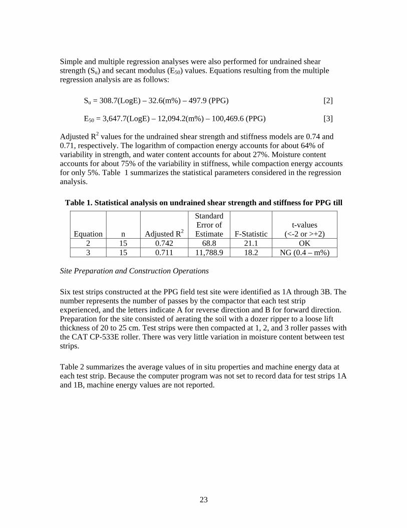
23

Simple and multiple regression analyses were also performed for undrained shear strength (Su) and secant modulus (E50) values. Equations resulting from the multiple regression analysis are as follows:

Su = 308.7(LogE) – 32.6(m%) – 497.9 (PPG) [2]

E50 = 3,647.7(LogE) – 12,094.2(m%) – 100,469.6 (PPG) [3] Adjusted R2 values for the undrained shear strength and stiffness models are 0.74 and 0.71, respectively. The logarithm of compaction energy accounts for about 64% of variability in strength, and water content accounts for about 27%. Moisture content accounts for about 75% of the variability in stiffness, while compaction energy accounts for only 5%. Table 1 summarizes the statistical parameters considered in the regression analysis.

Table 1. Statistical analysis on undrained shear strength and stiffness for PPG till

Equation n Adjusted R2

Standard Error of Estimate F-Statistic

t-values (<-2 or >+2)

2 15 0.742 68.8 21.1 OK 3 15 0.711 11,788.9 18.2 NG (0.4 – m%)

Site Preparation and Construction Operations

Six test strips constructed at the PPG field test site were identified as 1A through 3B. The number represents the number of passes by the compactor that each test strip experienced, and the letters indicate A for reverse direction and B for forward direction. Preparation for the site consisted of aerating the soil with a dozer ripper to a loose lift thickness of 20 to 25 cm. Test strips were then compacted at 1, 2, and 3 roller passes with the CAT CP-533E roller. There was very little variation in moisture content between test strips.

Table 2 summarizes the average values of in situ properties and machine energy data at each test strip. Because the computer program was not set to record data for test strips 1A and 1B, machine energy values are not reported.

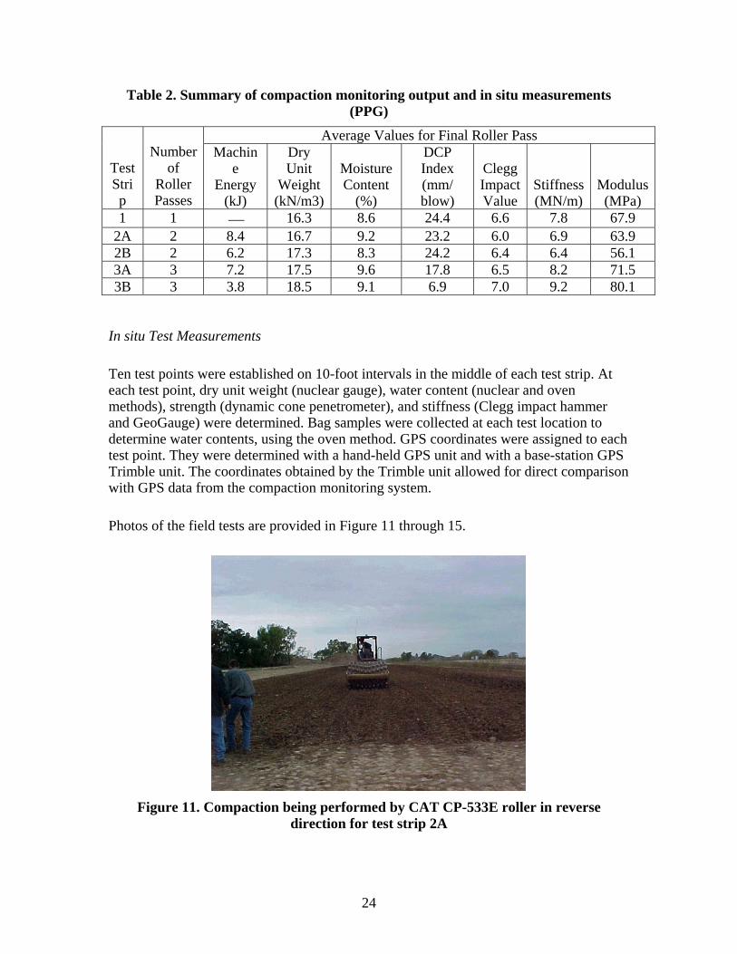
24

Table 2. Summary of compaction monitoring output and in situ measurements (PPG)

Average Values for Final Roller Pass

Test Strip

Number of

Roller Passes

Machine

Energy (kJ)

Dry Unit

Weight (kN/m3)

Moisture Content

(%)

DCP Index (mm/ blow)

Clegg Impact Value

Stiffness (MN/m)

Modulus(MPa)

1 1 ⎯ 16.3 8.6 24.4 6.6 7.8 67.9 2A 2 8.4 16.7 9.2 23.2 6.0 6.9 63.9 2B 2 6.2 17.3 8.3 24.2 6.4 6.4 56.1 3A 3 7.2 17.5 9.6 17.8 6.5 8.2 71.5 3B 3 3.8 18.5 9.1 6.9 7.0 9.2 80.1


Ten test points were established on 10-foot intervals in the middle of each test strip. At each test point, dry unit weight (nuclear gauge), water content (nuclear and oven methods), strength (dynamic cone penetrometer), and stiffness (Clegg impact hammer and GeoGauge) were determined. Bag samples were collected at each test location to determine water contents, using the oven method. GPS coordinates were assigned to each test point. They were determined with a hand-held GPS unit and with a base-station GPS Trimble unit. The coordinates obtained by the Trimble unit allowed for direct comparison with GPS data from the compaction monitoring system.

Photos of the field tests are provided in Figure 11 through 15.

Figure 11. Compaction being performed by CAT CP-533E roller in reverse

direction for test strip 2A

25

Figure 12. Trimble GPS base-station system used in situ test point locations

Figure 13. CIV stiffness measurements using the Clegg impact hammer

26

Figure 14. GeoGauge stiffness measurements

Figure 15. DCP strength profile measurements

Compaction Monitoring Output Results

Compaction monitoring results for the PPG field test strips are shown in Figure 16 and 17. The consolidation screen (Figure 16) displays the machine response after 2 and 3 passes for test sections 2 and 3. The reference color bar on the right side of the figure indicates machine power scale with a color transition from red (low compaction) to green (high compaction). Cell colors in test strip 2 were mostly yellow with spots of red and green. Colors in test strip 3 were mostly green with spots of yellow and red. Based on color changes, it can be determined that machine power was dissipating with increasing coverage. However, some areas of red (low compaction) still existed.

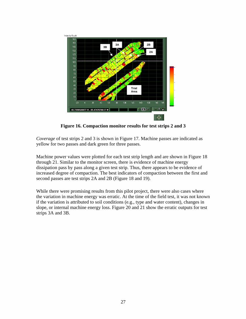
27

Figure 16. Compaction monitor results for test strips 2 and 3

Coverage of test strips 2 and 3 is shown in Figure 17. Machine passes are indicated as yellow for two passes and dark green for three passes.

Machine power values were plotted for each test strip length and are shown in Figure 18 through 21. Similar to the monitor screen, there is evidence of machine energy dissipation pass by pass along a given test strip. Thus, there appears to be evidence of increased degree of compaction. The best indicators of compaction between the first and second passes are test strips 2A and 2B (Figure 18 and 19).

While there were promising results from this pilot project, there were also cases where the variation in machine energy was erratic. At the time of the field test, it was not known if the variation is attributed to soil conditions (e.g., type and water content), changes in slope, or internal machine energy loss. Figure 20 and 21 show the erratic outputs for test strips 3A and 3B.

3B3A 2B

2A

Trial Area

28

Figure 17. Coverage monitor results for test strips 2 and 3

0

15

30

45

0 10 20 30

Location (m)

Mac

hine

Ene

rgy

(kJ)

Pass 1Pass 2

Figure 18. Machine power values as a function of roller pass for test strip 2A at

Peoria Proving Grounds

3B3A 2B

2A

Trial Area

9 8 7 6 5 4 3 2 1

29

0

15

30

45

0 10 20 30

Location (m)

Mac

hine

Ene

rgy

(kJ)

Pass 1Pass 2

Figure 19. Machine power values as a function of roller pass for test strip 2B at


0

15

30

45

0 10 20 30

Location (m)

Mac

hine

Ene

rgy

(kJ)

Pass 1Pass 2Pass 3

Figure 20. Machine power values as a function of roller pass for test strip 3A at


30

0

15

30

45

0 10 20 30

Location (m)

Mac

hine

Ene

rgy

(kJ)

Pass 1Pass 2Pass 3

Figure 21. Machine power values as a function of roller pass for test strip 3B at


Regression Analysis

The CAT compaction monitoring system relies on a net power value and number of roller passes as an indicator of compaction. Thus, testing the numeric relationship between the soil properties and net power value was determined to be a good starting point for the evaluation.

The regression analysis included the following steps:

• Enter data into ArcGIS, a geographic information system software package by ESRI.

• Group power data by the number of passes for each test strip using ArcMap, the mapping module in ArcGIS.

• Determine engine power values for each test strip. • Match power point values with the corresponding test points. • Calculate means for the power data (i.e., net power and gross power) and soil

properties (e.g., moisture content, dry density, and MDCP) for each unit section. • Calculate two to ten unit section moving averages using unit section mean power

and soil property values. • Plot paired scatter plots to observe trends and propose regression models. • Perform simple and multiple linear regression analyses using a data set for each

moving average span.

31

• Summarize findings. A two unit (20 ft) to ten unit (100 ft) moving average method was used to evaluate the minimum test strip size to develop an accurate regression model. One problem with this type of regression method is that larger unit sections overlap, potentially causing auto-correlation problems. Theoretically, this is not a proper treatment of data for regression analysis because the independent error assumption is violated. However, the analysis result is still reported here simply to show that with an increased number of unit section lengths, a higher regression correlation can be obtained between power values and soil properties.

In this analysis, net power was considered the prime indicator for correlation to soil properties. Based on patterns observed from the paired scatter plot (refer to “Paired Scatter Plot” in Part I of Appendix B), the following regression models were tested:

• Model A: Dry Density (DD) = Net Power (NP) • Model B: DD = Log (NP) • Model C: DD = Log(NP) + Moisture Content (MC) • Model D: CIV = NP • Model E: CIV = Log(NP) + MC • Model F: CIV = Log(NP) + MC

Table 3 shows the probabilities that the coefficients for power items are equal to zero. When these coefficients are zero, it means that the soil properties do not have a significant relationship with the power values. Generally, when the probability value is below 5%, it can be asserted that the coefficient is not zero. Otherwise, there is no sufficient evidence to say that the coefficients are not zero (correlations between the power values and the soil properties are weak or non-existent). According to Table 3, when using the unit section means for regression (MA Span = 1), the correlation between soil properties and net power values is weak. The correlations become stronger as the MA span increases (i.e., including a larger test area in the regression analysis).

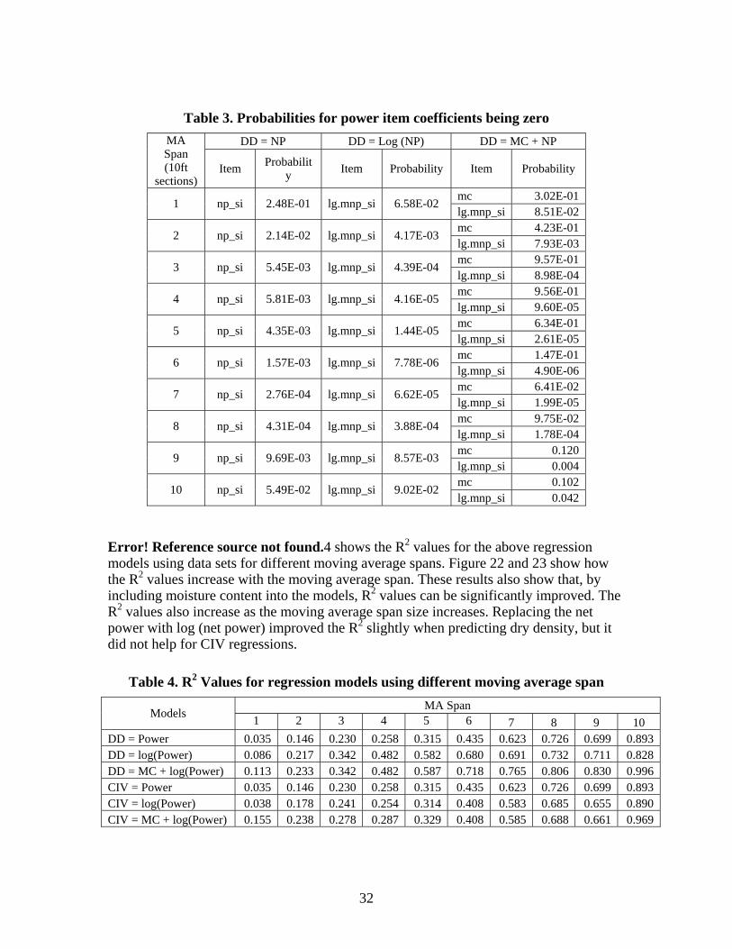
32

Table 3. Probabilities for power item coefficients being zero

DD = NP DD = Log (NP) DD = MC + NP MA Span (10ft

sections) Item Probabilit

y Item Probability Item Probability

mc 3.02E-01 1 np_si 2.48E-01 lg.mnp_si 6.58E-02 lg.mnp_si 8.51E-02 mc 4.23E-01 2 np_si 2.14E-02 lg.mnp_si 4.17E-03 lg.mnp_si 7.93E-03 mc 9.57E-01 3 np_si 5.45E-03 lg.mnp_si 4.39E-04 lg.mnp_si 8.98E-04 mc 9.56E-01 4 np_si 5.81E-03 lg.mnp_si 4.16E-05 lg.mnp_si 9.60E-05 mc 6.34E-01 5 np_si 4.35E-03 lg.mnp_si 1.44E-05 lg.mnp_si 2.61E-05 mc 1.47E-01 6 np_si 1.57E-03 lg.mnp_si 7.78E-06 lg.mnp_si 4.90E-06 mc 6.41E-02 7 np_si 2.76E-04 lg.mnp_si 6.62E-05 lg.mnp_si 1.99E-05 mc 9.75E-02 8 np_si 4.31E-04 lg.mnp_si 3.88E-04 lg.mnp_si 1.78E-04 mc 0.120 9 np_si 9.69E-03 lg.mnp_si 8.57E-03 lg.mnp_si 0.004 mc 0.102 10 np_si 5.49E-02 lg.mnp_si 9.02E-02 lg.mnp_si 0.042

Error! Reference source not found.4 shows the R2 values for the above regression models using data sets for different moving average spans. Figure 22 and 23 show how the R2 values increase with the moving average span. These results also show that, by including moisture content into the models, R2 values can be significantly improved. The R2 values also increase as the moving average span size increases. Replacing the net power with log (net power) improved the R2 slightly when predicting dry density, but it did not help for CIV regressions.

Table 4. R2 Values for regression models using different moving average span MA Span Models 1 2 3 4 5 6 7 8 9 10

DD = Power 0.035 0.146 0.230 0.258 0.315 0.435 0.623 0.726 0.699 0.893 DD = log(Power) 0.086 0.217 0.342 0.482 0.582 0.680 0.691 0.732 0.711 0.828 DD = MC + log(Power) 0.113 0.233 0.342 0.482 0.587 0.718 0.765 0.806 0.830 0.996 CIV = Power 0.035 0.146 0.230 0.258 0.315 0.435 0.623 0.726 0.699 0.893 CIV = log(Power) 0.038 0.178 0.241 0.254 0.314 0.408 0.583 0.685 0.655 0.890 CIV = MC + log(Power) 0.155 0.238 0.278 0.287 0.329 0.408 0.585 0.688 0.661 0.969

33

0.0

0.2

0.4

0.6

0.8

1.0

1.2

1 2 3 4 5 6 7 8 9 10

Moving Average Span

R2

DD = Pow erDD = log(Pow er)

DD = MC + log(Pow er)

Figure 22. R2 versus moving average span for models predicting dry density

0.0

0.2

0.4

0.6

0.8

1.0

1.2

1 2 3 4 5 6 7 8 9 10

Moving Average Span

R2

CIV = Pow erCIV = log(Pow er)

CIV = MC + log(Pow er)

Figure 23. R2 versus moving average span for models predicting CIV

34

Key Findings and Recommendations – Project No. 1.

In this field test, three test sections, each with two test strips (forward and reverse machine direction), were compacted with one, two, or three passes, respectively. Test strip one data was not included in the analysis because the machine data was not properly recorded. In situ soil property measurements, including dry density, moisture content, Clegg impact value, and DCP, were measured after the last pass of the respective test strips. To test how well the CAT compaction monitoring system performed, soil properties were regressed with net power values collected by the monitoring system. A moving average method was used to find the optimal length of unit sections. The regression results show that, when a small unit section length (10 ft) is used, the correlations between the soil properties and the net power value are weak. As the unit section length increases, the relationship between the net power and the soil properties improves.

Two possible reasons may exist for the poor performance of net power in predicting soil properties using small unit section lengths: (1) an insufficient number and variation in situ test results were provided for the regression and (2) the machine response was masking the true variability in changing soil conditions.

It is recommended that the highly erratic behavior in the machine power values be addressed. For future testing, it is also recommended to evaluate the compaction monitoring response to variations in moisture contents and loose lift thicknesses.

35

Project No. 2 – Caterpillar Edwards Facility Field Test

This project report summarizes field measurements and analyses for data collected during the March 24-26, 2004, pilot study at the indoor CAT Edwards Facility near Peoria, IL.


Soil at this test site was relatively uniform and of glacial origin. Classification tests identified the soil as sandy lean clay (CL) with a liquid limit of 29% and plasticity index of 13%. The maximum dry unit weight at standard Proctor compaction is 18.8 kN/m3 and optimum moisture content is about 12%. The percent passing the No. 200 sieve is approximately 69%. The specific gravity of the soil solids was determined to be 2.70.

Figure 24 presents the results of Proctor compaction tests for compaction energy levels of 355, 592, 987, 1463, and 2693 kJ/m3. Indicated on this figure are the zero air void curve and degree of saturation lines from 50% to 100% in increments of 10%. The results show that increased compaction energy increases the maximum dry unit weight and decreases the optimum moisture content.

16

17

18

19

20

21

5.0 10.0 15.0 20.0Moisture Content, (%)

Dry

Uni

t Wei

ght,

(kN

/m3 )

355

592987

1643

2693ZAV curve

Indicate % sat. in increments of 10%


Figure 24. Laboratory compaction test results on Edwards till for various

compaction energies

36

Figure 25 shows the linear correlation between the logarithm of compaction energy, maximum dry unit weight, and optimum moisture content. An R2 value of 0.96 for maximum dry unit weight versus compaction energy and an R2 value of 0.89 for optimum moisture content versus compaction energy show a strong linear correlation. Maximum dry unit weights and optimum water contents occurred between 85% and 90% saturation for this soil. Below 85% saturation, dry unit weight decreases with decreasing moisture content. Above 90% saturation, dry unit weight decreases with increasing moisture content.

y = -2.0757Ln(x) + 25.315R2 = 0.8918

y = 1.2477Ln(x) + 11.015R2 = 0.9593

8.0

10.0

12.0

14.0

16.0

18.0

20.0

22.0

100 1000 10000


Opt

imum

Wat

er C

onte

nt (%

) and

Max

imum

Dry

U

nit W

eigh

t (kN

/m3 )

Optimum MoistureContent

Maximum Dry UnitWeight

Figure 25. Semi-logarithmic relationship between compaction energy, optimum

water content, and maximum dry unit weight (Edwards till)

Figure 26 shows the relationship between dry unit weight and the logarithm of compaction energy for all compaction energies (Figure 24). Plotting the results in this way shows that achieving 100% standard Proctor compaction is only possible for moisture contents ≤ 15%. Furthermore, in order to achieve 100% standard Proctor compaction at moisture contents dry of optimum (≤ 12%), compaction energy must be greater than 987 kJ/m3. The effect that moisture content and compaction energy have on relative compaction is also shown in Figure 27, indicating that, at high water contents, no level of compaction energy will provide the desired level of relative compaction.

Results of the Proctor compaction tests were further evaluated statistically using multiple regression analyses. These analyses were performed not only to derive relationships for estimating the dry unit weight, but also to enable an understanding of factors contributing to variation in dry unit weight. The following equation resulted from the analyses:

37

DD = 2.92(Log E) - 0.02(m%) + 10.0 [1] In this equation, DD is the dry unit weight, E is the compaction energy, and m% is the percent moisture content (gravimetric). The adjusted R2 value for this analysis is 0.76. Logarithm of energy accounts for about 77% of the variability in the dry unit weight, while moisture content accounts for 8%. Other summary statistics are shown in Table 5.

16

17

18

19

20

21

100 1000 10000


Dry

Uni

t Wei

ght (

kN/m

3 )

7.69.611.713.315.25.917.7


100% StandardProctor Energy

Figure 26. Influence of compaction energy on dry unit weight as a function of

moisture content (Edwards till)

38

0

500

1000

1500

2000

2500

3000

0 5 10 15 20


Ene

rgy

(kJ)

100% SP95% SP100% MP95% MP97.5% MP

Figure 27. Energy as a function of moisture content for various degrees of

compaction (Edwards till)

Table 5. Statistical analysis on dry unit weight for Edwards till




1 26 0.755 0.51 39.6 NG (0.5 – m%) Soil Strength and Stiffness

Figure 28 and 29 show the undrained shear strength and stiffness (secant modulus) of the Edwards till as a function of the logarithm of compaction energy. The highest strength values were measured for water contents ≤ 12%. In general, increased compaction energy increases strength for water contents less than optimum, but does not increase strength for water contents greater than optimum. Stiffness values also increase with increasing compaction energy, but only for water contents well below optimum (5%). For moisture contents at optimum and wetter, increased compaction energy exhibits little influence on stiffness. In fact, close examination of Figure 29 shows that stiffness decreases with increased compaction energy for water contents just below and above optimum. Figure C.1 in Appendix C displays the corresponding dry unit weights of unconfined compression test specimens. Figures C.2–C.10 in Appendix C show stress-strain compression test results comparatively between energy levels at similar moisture contents and between moisture contents at the same energy levels.

39

0

100

200

300

400

500

600

100 1000 10000

Compaction Engery, (kJ/m3)

Und

rain

ed S

hear

Stre

ngth

, (kP

a)

5.3

8.6

11.2

13.9


Figure 28. Semi-logarithmic relationship between undrained shear strength and

compaction energy as a function of water content (Edwards till)

0

40000

80000

120000

160000

200000

100 1000 10000

Energy (kJ/m3)

Sec

ant M

odul

us, E

50 (k

Pa)

5.3

8.6

11.2

13.9


Figure 29. Semi-logarithmic relationship between secant modulus and compaction

energy as a function of water content (Edwards till)

40

Multiple regression analyses were also performed for undrained shear strength (Su) and secant modulus (E50). The following set of equations resulted from the analyses:

Su = 326(Log E) – 15.5(m%) – 577 [2] E50 = 41262(Log E) – 8062(m%) – 2362 [3]

Adjusted R2 values for the undrained shear strength and stiffness models are 0.74 and 0.54, respectively. For strength, the logarithm of energy accounts for more of the variability, at 63%, while moisture content explains about 17% of the variation. In contrast, moisture content explains about 47% of the variability in stiffness, while compaction energy only explains about 14%. Other summary statistics are displayed in Table 6.

Table 6. Statistical analysis on strength and stiffness for Edwards till




2 19 0.737 69.0 26.3 OK 3 19 0.539 26,292.2 11.5 OK

Site Preparation and Compaction Operations

Eight test strips, identified as A through H, were constructed and tested. Construction operations consisted of the following steps: (1) aerate/till existing soil with an RR350, (2) moisture condition soil with water truck, (3) remix with 1 to 2 additional passes of the RR350, (4) blade to level surface, and (5) compact with 6 to 10 passes of the CAT CP-533E roller. The test strips varied in loose lift thickness and water content. Table 7 summarizes the average values of lift thickness, number of passes, in situ test results, and machine energy values for each test strip. Tests results on a point-by-point basis are provided in Appendix C.

41

Table 7. Summary of compaction monitoring output and in situ measurements (Edwards Test Facility)

Average Values for Final Roller Pass

Test Strip

Loose Lift

Thickness (cm)

Number of

Roller Passes

Machine Energy

(kJ)

Dry Unit

Weight (kN/m3)

Moisture Content

(%)

DCP Index

(mm/blow)

Clegg Impact Value

A 30 6 33.3 17.48 9.5 24 13.0 B 40 6 36.1 17.24 13.6 47 9.0 C 40 6 33.4 17.87 15.4 80 5.7 D 40 6 39.6 17.67 15.7 81 5.1 F 68 10 30.4 18.11 15.6 60 7.6 G 68 10 26.1 18.53 12.8 41 11.6 H 30 10 20.52 19.09 12.8 25 13.0

Test strips A through D were compacted first. Test strips F through G were compacted in the forward and reverse directions, and test strip H was compacted with 10 passes in the forward direction only.


To evaluate changes in soil properties with compaction, 5 to 10 test points were randomly identified within each test strip and measured for density (nuclear and drive core methods), water content (nuclear, oven, and time-domain reflectometry methods), strength (dynamic cone penetrometer), and stiffness (Clegg impact hammer). At each test point, it was noted if the test location was within or out of the rear roller wheel paths.

Drive core and/or bag samples were collected at each test location to determine water contents, using the oven method. Density comparisons were also made by comparing the drive core density values with the in situ nuclear density measurements. Figure 30 shows that the drive core samples generally yield a higher density. The drive core samples were taken in the top 5 to 13 cm, whereas the nuclear tests averaged a measurement over the top 20 to 30 cm. Shallower nuclear tests (i.e., 10, 15, 20 cm) also show higher density values near the surface (Figure 31). This finding suggests that the compaction effort was not reaching the full depth of the loose lift.

42

15

16

17

18

19

20

15 16 17 18 19 20

Nuclear Dry Unit Weight (kN/m3)

Driv

e C

ore

Dry

Uni

t Wei

ght (

kN/m

3 )

Figure 30. Comparison of drive core and nuclear density values

0

5

10

15

20

25

30

35

16 17 18 19Dry Unit Weight (kN/m3)

Dep

th (c

m)

Point 7Point 8Drive Core

Figure 31. Depth versus density results for nuclear gauge (Test Strip C)

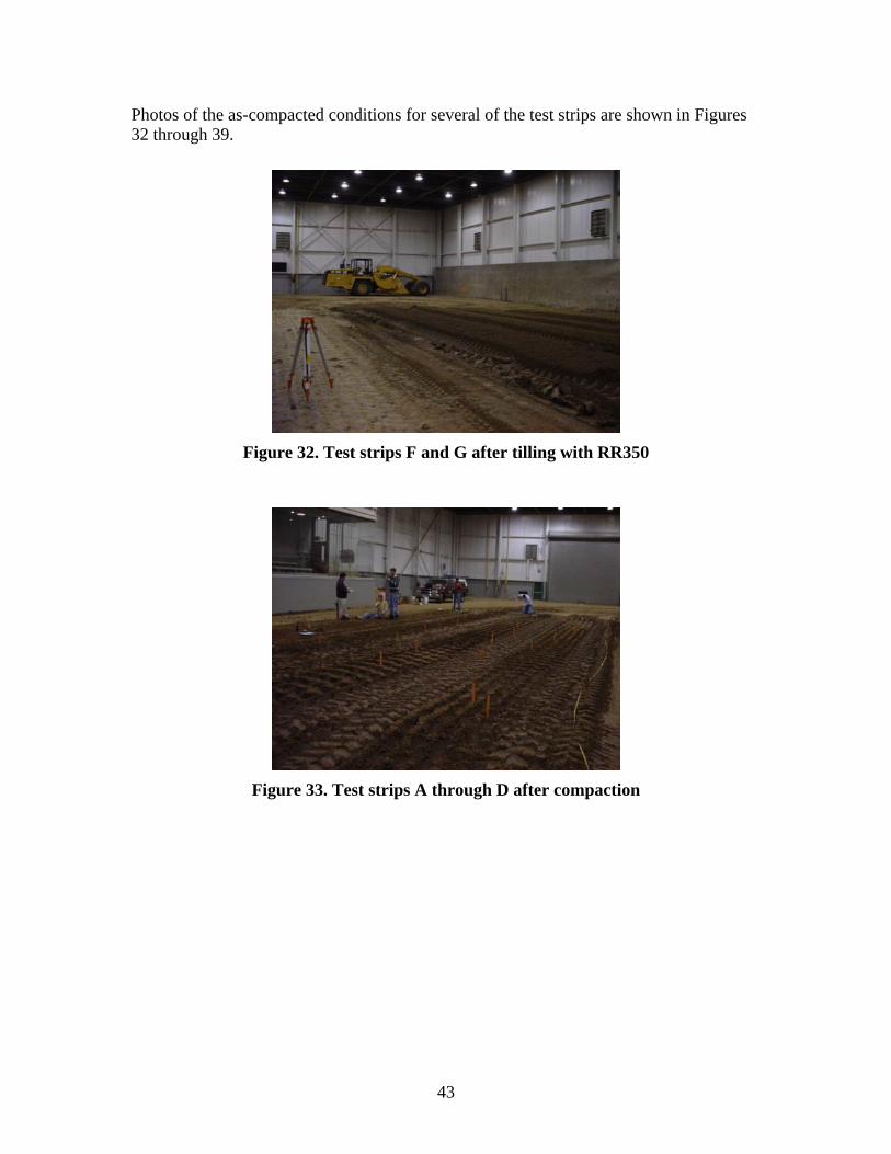
43

Photos of the as-compacted conditions for several of the test strips are shown in Figures 32 through 39.

Figure 32. Test strips F and G after tilling with RR350

Figure 33. Test strips A through D after compaction

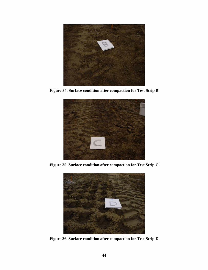
44

Figure 34. Surface condition after compaction for Test Strip B

Figure 35. Surface condition after compaction for Test Strip C

Figure 36. Surface condition after compaction for Test Strip D

45

Figure 37. Surface condition after compaction for Test Strip E

Figure 38. Surface condition after compaction for Test Strip F

Figure 39. Surface condition after compaction for Test Strip G

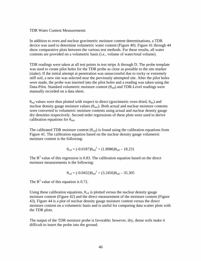
46

TDR Water Content Measurements

In addition to oven and nuclear gravimetric moisture content determinations, a TDR device was used to determine volumetric water content (Figure 40). Figure 41 through 44 show comparative plots between the various test methods. For these results, all water contents are provided on a volumetric basis (i.e., volume of water/total volume).

TDR readings were taken at all test points in test strips A through D. The probe template was used to create pilot holes for the TDR probe as close as possible to the site marker (stake). If the initial attempt at penetration was unsuccessful due to rocky or extremely stiff soil, a new site was selected near the previously attempted site. After the pilot holes were made, the probe was inserted into the pilot holes and a reading was taken using the Data-Pilot. Standard volumetric moisture content (θstd) and TDR-Level readings were manually recorded on a data sheet.

θstd values were then plotted with respect to direct (gravimetric oven dried, θdir) and nuclear density gauge moisture values (θnuc). Both actual and nuclear moisture contents were converted to volumetric moisture contents using actual and nuclear density gauge dry densities respectively. Second order regressions of these plots were used to derive calibration equations for θstd.

The calibrated TDR moisture content (θcal) is found using the calibration equations from Figure 41. The calibration equation based on the nuclear density gauge volumetric moisture content is the following:

θcal = (-0.0187)θstd2 + (1.8986)θstd – 18.231

The R2 value of this regression is 0.83. The calibration equation based on the direct moisture measurements is the following:

θcal = (-0.0432)θstd2 + (3.2456)θstd – 35.305

The R2 value of this equation is 0.72.

Using these calibration equations, θcal is plotted versus the nuclear density gauge moisture content (Figure 42) and the direct measurement of the moisture content (Figure 43). Figure 44 is a plot of nuclear density gauge moisture content versus the direct moisture content on a volumetric basis and is useful for comparing data scatter plots with the TDR plots.

The output of the TDR moisture probe is favorable; however, dry, dense soils make it difficult to insert the probe into the ground.

47

Figure 40. TDR equipment

y = -0.0432x2 + 3.2456x - 35.305R2 = 0.7236

y = -0.0187x2 + 1.8986x - 18.231R2 = 0.8277

10

15

20

25

30

35

10 20 30 40 50

TDR std. calibration volumetric water content (%)

Nuc

lear

and

ove

n vo

lum

etric

wat

er c

onte

nt (%

)

Nuclear vs. TDR

Actual vs. TDR

Figure 41. TDR vs. nuclear and oven volumetric water contents (%)

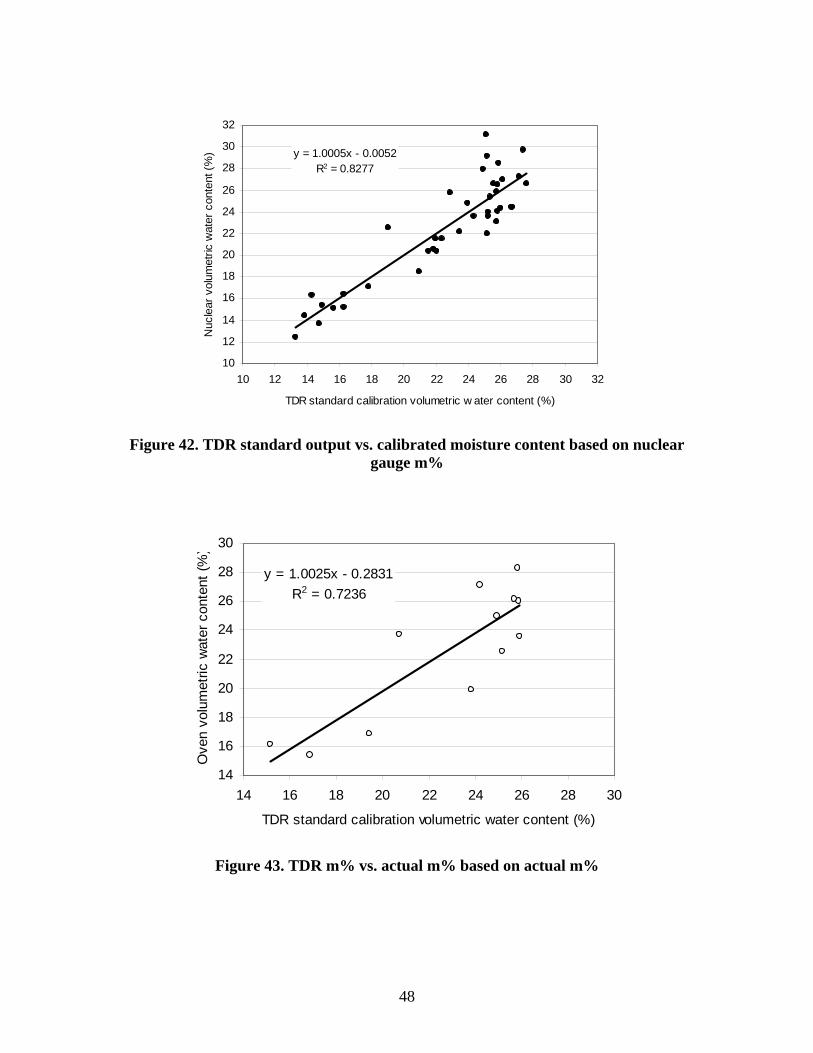
48

y = 1.0005x - 0.0052R2 = 0.8277

10

12

14

16

18

20

22

24

26

28

30

32

10 12 14 16 18 20 22 24 26 28 30 32

TDR standard calibration volumetric w ater content (%)

Nuc

lear

vol

umet

ric w

ater

con

tent

(%)

Figure 42. TDR standard output vs. calibrated moisture content based on nuclear

gauge m%

y = 1.0025x - 0.2831R2 = 0.7236

14

16

18

20

22

24

26

28

30

14 16 18 20 22 24 26 28 30

TDR standard calibration volumetric water content (%)

Ove

n vo

lum

etric

wat

er c

onte

nt (%

)

Figure 43. TDR m% vs. actual m% based on actual m%

49

y = 1.0655x + 0.2304R2 = 0.8523

4.0

6.0

8.0

10.0

12.0

14.0

16.0

18.0

20.0

4 6 8 10 12 14 16 18 20

Oven volumetric water content (%)

Nuc

lear

vol

umet

ric w

ater

con

tent

(%)

Figure 44. Nuclear versus oven on volumetric basis

DCP Test Results

Dynamic Cone Penetrometer (DCP) tests were performed at all test points to develop strength versus depth profiles. Table 8 summarizes the average water content, average loose lift thickness, average compacted lift thickness, and the average MDCP index results for each test strip. Individual DCP test results are provided in Appendix C.

Compacted lift thicknesses were obtained from the DCP plots by observing the change in the DCP index profile with depth. The MDCP index was calculated by averaging the index values in the uppermost lift and ignoring results from the underlying layer.

In relation to strength, in this case California Bearing Ratio (CBR), the DCP index values decrease with increasing CBR. Figure 45 shows that the DCP index values increase with increasing water content. Figure 46 shows the scattered influence of lift thickness on MDCP index.

50

Table 8. MDCP index test results

Test Strip A B C D E F G H Average w% 9.5 12.2 15.4 17.3 8.9 15.6 12.8 12.9

Average Loose lift(in)

12 16 16 16 10 26-28 26 12

Average Compacted Lift(in)

10.1 9.8 10 10.1 7.4 17.8 21.2 6.4

Test Point MDCP index (mm/blow) 1 12 45 53 34 12 59 47 25 2 17 52 116 55 18 60 41 28 3 37 50 116 93 10 69 41 22 4 20 49 66 71 19 49 38 28 5 15 44 90 92 12 57 38 36 6 28 50 91 87 16 95 ⎯ 24 7 28 48 63 76 26 56 ⎯ 17 8 32 43 90 100 17 47 ⎯ 34 9 19 49 68 130 16 54 — 20 10 31 39 51 73 9 49 — 17

Average 24 47 80 81 15 60 41 25

y = 7.8716x - 56.646R2 = 0.8078

0

20

40

60

80

100

120

140

5 10 15 20

Moisture (%)

Avg

MD

CP

(mm

/blo

w)

Figure 45. Average MDCP index vs. moisture

51

0

20

40

60

80

100

120

140

0 5 10 15 20 25

Lift thickness (inches)

Ave

rage

MD

CP

(mm

/blo

w)

Figure 46. Average MDCP index vs. lift thickness

Observations of the individual DCP plots in Appendix C reveal that all test strips, with the exception of H, show significant “Oreo cookie” profiles. The top part (crust) is dense and the bottom is soft. This is observed in most plots but is more pronounced for the larger lift thicknesses (see Figure 47).

0

5

10

15

20

25

30

35

40

1 10CBR

DEP

TH, i

n.

0

100

200

300

400

500

600

700

800

900

10001 10 100

DEP

TH, m

m

Figure 47. CBR plot of test point 4 from test strip F

52

Stiffness

Clegg Impact Values (CIV) are empirically related to CBR and soil stiffness parameters (i.e., modulus of subgrade reaction) and can simulate penetration of a roller pad/foot. Figure 48 shows that the CIV increases as the water content decreases.

y = -1.4869x + 30.111R2 = 0.7823

0

5

10

15

20

25

30

35

5 10 15 20

Gravimetric Water Content (%), Nuclear Measurements

Cle

gg Im

pact

Val

ue (C

IV)

Figure 48. Influence of water content on CIV measurements


Transitions from red to green were observed on the consolidation screen of the cab display monitor: red indicated areas of higher machine power and green indicated lower machine power. Color coded changes were clearly seen on the coverage screen, transitioning from yellow to red with increased number of roller passes. Yellow indicates one pass and red indicates ten or more passes. All test strips were compacted until the consolidation screen indicated green throughout the majority of the test strip area. Once this threshold was achieved, the soil was considered compacted, and the in situ comparison field tests were performed. Figure 49 and 50 show screen captures from the compaction monitor for test strip H for consolidation and coverage. Similar screen captures are provided in Appendix C.

Figure 49 shows the consolidation results for 1, 4, and 10 roller passes. As shown, the consolidation display shows areas of red (low compaction) for pass number one, but with increased number of passes, the output transitions from red to green, indicating a higher degree of compaction. Figure 50 shows the corresponding coverage area (number of passes) for 1, 4, and 10 roller passes.

53

(a)

(b)

(c)

Figure 49. Monitor output for machine energy after 1, 4, and 10 roller passes (a – c) on test strip H at Edwards Test Facility

54

(a)

(b)

(c)

Figure 50. Monitor output for machine coverage after 1, 4, and 10 roller passes (a – c) on test strip H at Edwards Test Facility

55

Machine response to the soil was evaluated further by considering machine power values pass by pass along individual test strips. Similar to project no. 1, there continued to be good evidence of machine energy dissipation pass by pass along a given test strip, which is indicative of increased degree of compaction. Figures 51 and 52 show machine energy variation along the length of the test strips G and H, respectively.

In some cases, the variation in machine energy was erratic and may be attributed to variations in soil conditions (e.g., type and water content) or changes in slope or internal machine energy loss. Figure 53 and 54 show the most evident examples of variable output from test strips D and F.

0

20

40

60

80

0 3 6 9 12

Location (m)

Mac

hine

Ene

rgy

(kJ)

Pass 2Pass 4Pass 8Pass 10

Figure 51. Machine power values as a function of roller pass for test strip G at

Edwards Test Facility

56

0

20

40

60

80

0 5 10 15 20

Location (m)

Mac

hine

Ene

rgy

(kJ)


Figure 52. Machine power values as a function of roller pass for test strip H at


0

20

40

60

80

0 5 10 15 20

Location (m)

Mac

hine

Ene

rgy

(kJ)

Pass1

Pass 3

Pass 6

Figure 53. Machine power values as a function of roller pass for test strip D at


57

0

20

40

60

80

0 5 10 15 20Location (m)

Mac

hine

Ene

rgy

(kJ)


Figure 54. Machine power values as a function of roller pass for test strip F at


Exploratory Study of Compaction Monitoring Output

Box plots for engine power values were plotted as a function of the number of roller passes for each test strip. Box plots (Chambers 1983) are a statistical tool for conveying location and variation information in data sets and are particularly useful for detecting and illustrating location and variation changes between different groups of data. Five basic statistics are required to draw a box plot: the upper whisker, the third (upper) quartile, the median, the first (lower) quartile, and the lower whisker. The upper whisker is the lower of the maximum observation and the third quartile plus 1.5 times the interquartile range (the difference between the lower and the upper quartiles). The lower whisker is the higher of the minimum observation and the first quartile minus 1.5 times the interquartile range. The mean of the group of data was also added to a box plot.

A general trend between the engine power values and the number of passes can be observed from the box plots, as illustrated in Figure 55 and 56. On a level test strip, the gross power and net power values generally have a decreasing trend as the number of passes increases, but the difference between neighboring passes also decreases with the increase in number of passes. For box plots of gross power and net power for all test strips of field test two, refer to the “Box Plots” for “Measured Power Values” in Appendix D.

58

Figure 55. Box plots for gross power versus number of passes for test strip A

Figure 56. Box plots for net power versus number of passes for test strip A

Lower whisker

3rd Quartile Median

Mean

1st Quartile

Upper whisker

59

Variability of Power Values

Table 9 shows the summary statistics of standard deviation and coefficients of variation (COV) for gross and net power values for each roller pass. The COV is defined as the standard deviation of the net or gross power divided by the respective mean net or gross power values. The COV provides a measure of the relative variation in net or gross power for a given pass. The results indicate that the standard deviation for net power is smaller than that for the gross power (5.1 vs. 7.9), but the average COV value for net power is larger than that for the gross power (60% versus 20%).

Table 9. Summary statistics of coefficients of variation for gross and net power values

Standard Deviation Coefficient of Variation (%)

NP (KW) GP (KW) NP GP Mean 5.1 7.9 63 24 Median 4.6 7.1 65 19 Standard Deviation 2.4 5.5 22 22 Range 11.3 25.5 97 113 Minimum 1.0 1.4 3 2 Maximum 12.3 26.9 100 115 Count (Passes) 54

Figure 57 shows the distribution of standard deviation for net power values. One third (18 out of 54) of the net power values lies between 3 and 5. Three passes have standard deviation for net power over 9. The maximum standard deviation for net power is 12.4.

Figure 58 shows the distribution of standard deviation for gross power values. Of the 54 passes studied, one third (18 out of 54) of the passes have standard deviations below 5. Five passes have standard deviations over 17 and two passes over 23. The maximum standard deviation for gross power is 26.9.

60

0

2

4

6

8

10

12

14

16

18

20

3 5 7 9 11 13 More

Freq

uenc

y

Figure 57. Histogram for standard deviation for net power

0

2

4

6

8

10

12

14

16

18

20

5 8 11 14 17 20 23 26 29 More

Standard Deviation

Freq

uenc

y

Figure 58. Histogram for standard deviations for gross power

61

Figure 59 shows that, for most passes (about 85%), the COV for gross power lies between 10% and 40%. About 50% lie between 10% and 20%. Three passes have COV for gross power values over 90%, which may indicate highly variable soil conditions or erroneous machine response values. Figure 60 shows that most passes have COV values for net power between 30% and 100%.

0

5

10

15

20

25

30

0.1 0.2 0.3 0.4 0.5 0.6 0.7 0.8 0.9 1 1.1 More

Gross Power C.O.V. Values

Freq

uenc

y

Figure 59. Histogram of COV values for gross power

0

1

2

3

4

5

6

7

8

9

10

0.1 0.2 0.3 0.4 0.5 0.6 0.7 0.8 0.9 1 More

Net Power C.O.V. Values

Freq

uenc

y

Figure 60. Histogram of COV values for net power

62

Regression Analysis

To determine relationships between power output (gross and net) from the compaction monitoring system and various field measurements (density, DCP, and CIV), simple multiple linear regression analyses were performed. Further, because some field test points were located within the wheel path of the compactor, analyses were conducted to determine if measurements taken in the wheel path are significantly different from the ones taken between the wheel paths.

The regression analysis included the following steps:

• Enter data into ArcGIS, a Geographic Information System software package by ESRI.

• Group power data by the number of passes for each test strip using ArcMap, the mapping module in ArcGIS.

• Determine engine power values for each test strip. • Match power point values with the corresponding test points. • Calculate means for the power data (i.e., net power and gross power) and soil

properties (e.g., moisture content, dry density, and MDCP) for each unit section. • Plot paired scatter plots to observe trends and propose regression models. • Perform simple and multiple linear regression analyses. • Summarize findings.

A unit section is a data point in the regression analysis. To avoid autocorrelation between observations, moving averages of small unit sections (1/10 of the strip length) were not used in the regression analysis. Instead, two unit section lengths were used: 1/10 of the strip length (about 2 meters) and the length of the entire test strip (about 20 meters).

Based on findings from project no. 1, the following models were tested using both gross power and net power values to find out which one is a better indicator of soil properties.

• Model A: Dry Density (DD) = Power (Net Power or Gross Power) • Model B: DD = Log (Power) • Model C: DD = Log(Power) + Moisture Content (MC) • Model D: CIV = Power • Model E: CIV = Log(Power) + MC • Model F: CIV = Log(Power) + MC • Model F: MDCP = Power • Model G: MDCP = Log(Power) • Model H: MDCP = Log(Power) + MC

Complete results for the regression analysis for the second field test are shown in part I of Appendix D. Table 10 shows the R2 values for the different regression models using 1.8

63

m (6 ft) long unit sections. The results show that gross power has a moderate correlation with Dry Density, CIV, and MDCP (R2 values between 0.2 and 0.4). Meanwhile, the net power has a very low correlation with the Dry Density (R2 value 0.0014) but moderate correlations with the CIV and MDCP values (R2 values between 0.2 and 0.3). Including Moisture Content as an independent variable did not help for predicting the dry density but could improve models using CIV and MDCP as dependent variables.

Table 10. R2 values for different regression models using 6 ft long unit sections

Models GP NP DD = Power 0.3626 0.0014 DD = log(Power) 0.3988 7.2E-06 DD = MC + log(Power) 0.4057 0.0032 CIV = Power 0.2802 0.2259 CIV = log(Power) 0.2884 0.2152 CIV = MC + log(Power) 0.6969 0.5736 MDCP = Power 0.2229 0.2946 MDCP = log(Power) 0.2304 0.2371 MDCP = MC + log(Power) 0.7058 0.6331

Table 11 shows the R2 values for the regression analysis using an entire test strip as a unit section. The results show that Dry Density has a higher correlation with gross power than net power (0.83 versus 0.11), but CIV and MDCP have considerably higher correlations with the net power (0.70 and 0.66, respectively) than with the gross power (0.47 and 0.38, respectively).

Table 11. R2 values using an entire test strip as a unit section

Models GP NP DD = Power 0.8324 0.1138 DD = log(Power) 0.8620 0.1265 DD = MC + log(Power) 0.9336 0.2679 CIV = Power 0.4693 0.7007 CIV = log(Power) 0.4573 0.6930 CIV = MC + log(Power) 0.9726 0.8521 MDCP = Power 0.3838 0.6575 MDCP = log(Power) 0.3757 0.6087 MDCP = MC + log(Power) 0.9065 0.8040

The R2 values in Table 11 are considerably larger than those in Table 10. The high R2 values in Table 11 confirm that a significant relationship exists between soil properties and engine power output. This relationship, however, is of limited use in predicting the soil properties.

For project no. 2, some test point locations in and out of the wheel paths were measured and recorded. A two-sample t-tests analysis was conducted to test if there is significant difference in Dry Density, CIV, and DCP between points on the wheel path and the drum

64

path. The t-test included data collected from 65 test points. The t-test results, as shown in Table 12, reveal that mean dry densities between test points on drum paths and wheel paths are statistically different. The mean dry density is 17.26 kN/m3 for test points in the drum paths and 17.72 kN/m3 for points in the wheel paths. The difference is about 0.46 kN/m3, with a level of significance of 0.02. The CIV and the DCP values are not statistically different. The mean CIV is 8.61 for test points in the wheel paths and 9.84 for those in the drum paths. The difference is about 1.24. The MDCP is 55.7 mm/blow for points in the drum paths and 46.52 mm/blow for points in the wheel paths. The difference is about 9.2. The levels of significance for these two tests are 0.19 and 0.15. These results show that soil in the wheel paths does get more compaction that that in the drum paths. However, in real world construction where the wheel paths normally overlap with drum paths, the difference in compacted soil properties can make this a non-issue.

Table 12. Comparison of wheel path and drum path soil properties

Item Mean Std. Dev. Method t (equal

var.) P-value Significantly

Different? Drum path 17.263 0.823 DD

(KN/m3) Wheel path 17.719 0.729 Equal Var. -2.31 0.0242 Yes

Drum path 8.605 3.772 CIV Wheel path 9.844 3.651

Equal Var. -1.32 0.1908 No

Drum path 55.737 30.442 MDCP (mm/blow) Wheel path 46.519 21.212

Unequal Var. 1.44 0.1552 No

Key Findings and Recommendations – Project No. 2.

For project no. 2, eight test strips were compacted with 6 to 10 passes. In situ soil properties were tested for each test strip after the last pass. Box plots for the engine power values by number of passes show that a trend exists between the power values and the number of passes. Regression results show that significant correlations exist between dry density, CIV, MDCP, and gross power. Significant correlations also exist between CIV, MDCP, and net power. Unfortunately, the net power did not prove to be a good indicator of soil dry density. It is also not more efficient in predicting the CIV and MDCP than the gross power. Analysis of power values shows that the variability in net power is lower than gross power. The relative variability for net power, represented by COV, is almost 2.5 times that for gross power.

The trend in power values stimulates the interest to study whether similar trend exists in the soil properties as the number of passes increase. Thus, it is recommended that in situ soil properties be measured after each pass of compaction in future field tests.

The two field tests have demonstrated that this compaction monitoring technology has promise. In the first field test, we found that net power and moisture content were highly correlated to dry density using a 60 ft moving average of data. In the second field test, we found similar results but discovered that a significant dry density, strength, and stiffness relationship existed between gross power and moisture content using a shorter moving

65

average of data (about 40 ft). There appeared to be some improvement in the results from the second test, but it is difficult to explain why gross power would be a better indicator of soil properties than net power. Moreover, it was discovered that a significant difference exists for dry density values in the wheel path and out of the wheel path. This may indicate the need to reassess the algorithm that assigns power values (shown as different colors on the coverage screen) to each of the 1’ x 1’ cells. It appears that further refinement to this compaction monitoring technology is necessary.

The Iowa State University (ISU) research team would like to assist Caterpillar in refining its soil compaction monitoring technology by better understanding its “black box” in terms of its assumptions (e.g., net power transformation approach), equations, and data processing procedures. Each part of the “black box” needs to be carefully reviewed and understood, which might lead to important changes. It might be appropriate, for example, to solicit consultation from ISU Statistics Department, one of the best in the nation, to help analyze raw net power data and better understand the steady state and random nature of these data. Once this review is accomplished and appropriate modifications are made, then it would seem appropriate to expand the field testing effort.

66

Project No. 3 – Wells Fargo Headquarter Project, Des Moines, IA

This project report summarizes field measurements and preliminary analyses for data collected during the July 26-28, 2004, study at the Wells Fargo construction project in West Des Moines, IA.


Two similar soils (one existing and the other fill) were tested at the Wells Fargo project. Laboratory classification tests identify the soils as lean clays (CL). The existing on-site soil has a liquid limit of 42, a plasticity index of 10, and 99% pass the no. 200 sieve. The fill material has a liquid limit of 49, plasticity limit of 19, and 97% pass the no. 200 sieve.

Standard Proctor maximum dry unit weight is 16.2 kN/m3 for the on-site soil and 15.8 kN/m3 for the fill material. Optimum water contents are 20.0% and 26.0%, respectively. Specific gravities of the soils are about 2.70.

Proctor compaction test results for the soils are presented in Figure 61 and 62. Maximum dry unit weight and optimum water content occurred at approximately 85% saturation for both soils.

14

16

18

20

12.0 16.0 20.0 24.0 28.0

Moisture, (%)

Dry

Uni

t Wei

ght,

(kN

/m3 ) 592

ZAV

Compaction Energy, (kJ/m3)


Figure 61. Laboratory compaction test results on Des Moines clay 1 (natural on-site soil) for standard Proctor energy

67

12

14

16

18

20

18.0 20.0 22.0 24.0 26.0 28.0 30.0 32.0


Dry

Uni

t Wei

ght (

kN/m

3 ) 592ZAV

Indicate % sat.in increments of 10%

Figure 62. Laboratory compaction test results on Des Moines clay 2 (fill material)

for standard Proctor energy

Site Preparation and Compaction Operations

The Wells Fargo field tests were performed at three different areas on the project site. Soil at test strips A and B was disked with a tow-behind disk prior to compaction. Moisture contents were lower on test strip B due to aeration prior to compaction. Loose lift thicknesses for test strips A and B varied from 35 to 50 cm. The fill material test strips (C and CV) were disked and leveled to a loose lift thickness of about 40 cm. Compaction was performed with the CAT CP-533E roller. As recommended from project no. 2, in situ tests were performed between passes.

68

Table 13 through 16 summarize the average values of in situ test results and machine energy values for each pass.

Since previous tests had been conducted on relatively flat surfaces, test strip A was selected for the purpose of observing the compaction monitoring system’s response when compacting on a slope. Alternate passes were conducted with the roller going down and up the slope.

The vibratory option on the roller was also experimented with in regard to monitor response. Vibration was used on passes 7 and 8 for test strip B. A comparative analysis was performed on the fill material test strips, with one strip compacted with vibration (test strip CV) and the other without (test strip C). Test strips B, C, and CV were all compacted in the forward direction.

69

Table 13. Summary of compaction monitoring output and in situ measurements (West Des Moines - test strip A)

Average Values from Successive Roller Passes

Pass Number

Machine Energy

(kJ)

Dry Unit Weight (kN/m3)

Moisture Content

(%) DCP Index (mm/blow)

Clegg Impact Value

1 19.6 12.4 27.8 121 2.9 2 38.5 13.2 26.9 105 3.7 3 26.4 12.8 27.8 88 2.7 4 35.4 13.5 27.8 85 3.4

Table 14. Summary of compaction monitoring output and in situ measurements

(West Des Moines - test strip B)


Pass Number

Machine Energy

(kJ)


Moisture Content


Clegg Impact Value

1 60.0 13.2 25.4 150 2.8 2 47.7 13.5 22.4 151 3.1 3 48.2 13.5 22.0 109 3.6 4 42.6 14.2 21.3 102 3.8 6 37.6 14.5 21.9 120 3.8

8 (vibratory) 22.6 14.7 22.1 160 3.8

Table 15. Summary of compaction monitoring output and in situ measurements (West Des Moines - test strip C (no vibratory))


Pass Number

Machine Energy

(kJ)


Moisture Content


Clegg Impact Value

2 48.5 12.4 26.4 58 4.8 4 41.0 13.2 25.8 61 6.4 6 42.6 13.1 25.7 54 6.4

Table 16. Summary of compaction monitoring output and in situ measurements

(West Des Moines - test strip CV (vibratory))


Pass Number

Machine Energy

(kJ)


Moisture Content


Clegg Impact Value

2 47.4 12.6 28.8 56 6.1 4 37.3 13.4 28.0 51 6.9 6 39.0 13.5 24.7 48 6.9

70


Similar to project no. 2, in situ test points were randomly selected and measured for density (nuclear and drive core methods), water content (nuclear and oven methods), strength (dynamic cone penetrometer), and stiffness (Clegg impact hammer). A Trimble GPS base station system was again utilized to record in situ coordinates for later regression analysis.

Five test measurements were taken after each pass in test strips A and B. However, after pass 4 on test strip B, the measurements were taken every other pass. On strip C, three in situ measurements were taken after every two passes. Five measurements were taken after every two passes on strip CV.

Machine energy values are displayed in Figure 63 through 78 as a function of the number of roller passes. Here, the values were averaged and plotted on a semi-logarithmic scale versus the number of roller passes. A secondary axis was added to plot average in situ measurements. Results indicate trends of dry unit weight, percent compaction, and Clegg impact values (stiffness) increasing with decreasing machine energy values. There is also a slight trend in MDCP (strength) values decreasing with decreasing machine values. However, while the standard deviation is not plotted, the DCP values exhibited a high variation. Moreover, investigation of DCP profiles clearly show soft zones below the upper crust that were not compacted (i.e., “Oreo cookie” effect). This indicates that loose lifts constructed for the field tests were too thick for the pad-foot roller.

More importantly, this introduces a new problem to address ⎯ without the DCP profile, one was left to assume that efficient compaction had been performed based solely on the output from the consolidation monitor screen, i.e., on the appearance of green cells. This was not the case, however, due to the overly thick lifts. This finding emphasizes the importance of process control in addition to end-result measurements.

Dissipation of machine energy values was observed in test strips B, C, and CV with increased number of roller passes. Figures 67, 71, and 75 show trends between mean energy values and number of roller passes with relatively low variation. In some cases, (Figure 65) poor correlations and high variability are observed (strip A). The high variability in these examples appears to be related to negative energy values observed in the output. Negative machine values cannot be explained by the ISU research team. It has been proposed that perhaps the sloping ground conditions of test strip A were a contributor to the negative machine energy values. More research is needed to develop an explanation of this behavior.

Another note of interest is found in the results of the tests involving the vibratory option of the roller. Mean energy values in passes 7 and 8 of test strip B dropped significantly with vibratory option. Also, in situ measurements in test CV indicated denser and slightly stronger fill than in test strip C (non-vibratory). A comparison between the mean machine values for test strips C and CV shows them to be similar.

71

0

25

50

75

Number of Roller Passes

Mac

hine

Ene

rgy

(kJ)

14

15

16

Dry

Uni

t Wei

ght (

kN/m

3 )

Machine Energy Dry Unit Weight (Avg.)

2 3 4 5 6 7 8 9 101

Figure 63. Machine energy output and resulting dry unit weight as a function of

roller passes on test strip A

0

25

50

75


Mac

hine

Ene

rgy

(kJ)

85%

90%

95%

100%

% S

tand

ard

Pro

ctor

Machine Energy % Standard Proctor

2 3 4 5 6 7 8 9 10 1

Figure 64. Machine energy output and resulting percent standard Proctor as a

function of roller passes on test strip A

72

0

25

50

75


Mac

hine

Ene

rgy

(kJ)

0

60

120

180

DC

P (m

m/b

low

)

Machine Energy Mean DCP (Avg.)

2 3 4 5 6 7 8 9 10 1

Figure 65. Machine energy output and resulting MDCP as a function of roller

passes on test strip A

0

25

50

75


Mac

hine

Ene

rgy

(kJ)

0

2

4

6

8C

legg

Impa

ct V

alue

(CIV

)Machine Energy Clegg Value (Avg.)

2 3 4 5 6 7 8 9 101

Figure 66. Machine energy output and resulting CIV as a function of roller passes

on test strip A

73

0

25

50

75


Mac

hine

Ene

rgy

(kJ)

14

15

16

Dry

Uni

t Wei

ght (

kN/m

3 )


2 3 4 5 6 7 8 9 101

Figure 67. Machine energy output and resulting dry unit weight as a function of roller passes on test strip B

0

25

50

75


Mac

hine

Ene

rgy

(kJ)

85%

90%

95%

100%%

Sta

ndar

d P

roct

or


2 3 4 5 6 7 8 9 101


function of roller passes on test strip B

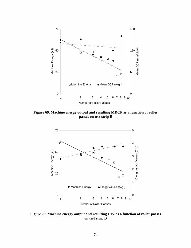
74

0

25

50

75

1 10


Mac

hine

Ene

rgy

(kJ)

0

60

120

180

Mea

n D

CP

(mm

/blo

w)


2 3 4 5 6 7 8 9


passes on test strip B

0

25

50

75

1 10


Mac

hine

Ene

rgy

(kJ)

0

1

2

3

4

5

Cle

gg Im

pact

Val

ues

(CIV

)

Machine Energy Clegg Values (Avg.)

2 3 4 5 6 7 8 9


on test strip B

75

0

25

50

75


Mac

hine

Ene

rgy

(kJ)

14

15

16

Dry

Uni

t Wei

ght (

kN/m

3 )


2 3 4 5 6 7 8 9 10 1


roller passes on test strip C (no vibration)

0

25

50

75


Mac

hine

Ene

rgy

(kJ)

85%

90%

95%

100%%

Sta

ndar

d P

roct

or


2 3 4 5 6 7 8 9 10 1


function of roller passes on test strip C (no vibration)

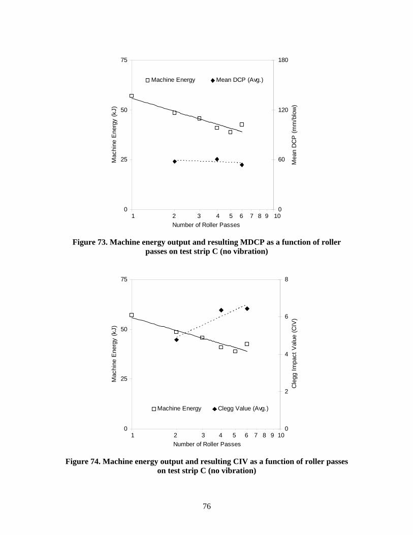
76

0

25

50

75


Mac

hine

Ene

rgy

(kJ)

0

60

120

180

Mea

n D

CP

(mm

/blo

w)


2 3 4 5 6 7 8 9 10 1


passes on test strip C (no vibration)

0

25

50

75


Mac

hine

Ene

rgy

(kJ)

0

2

4

6

8

Cle

gg Im

pact

Val

ue (C

IV)

Machine Energy Clegg Value (Avg.)

2 3 4 5 6 7 8 9 101


on test strip C (no vibration)

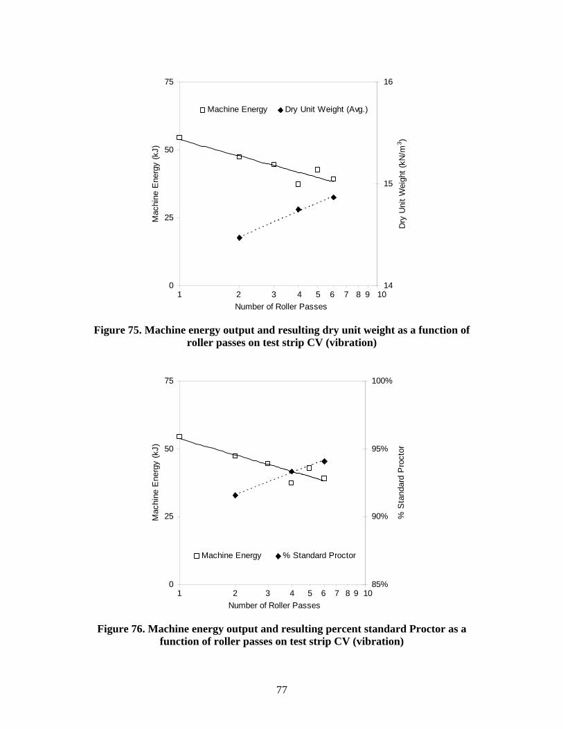
77

0

25

50

75


Mac

hine

Ene

rgy

(kJ)

14

15

16

Dry

Uni

t Wei

ght (

kN/m

3 )


2 3 4 5 6 7 8 9 101


roller passes on test strip CV (vibration)

0

25

50

75


Mac

hine

Ene

rgy

(kJ)

85%

90%

95%

100%

% S

tand

ard

Pro

ctor


2 3 4 5 6 7 8 9 101


function of roller passes on test strip CV (vibration)

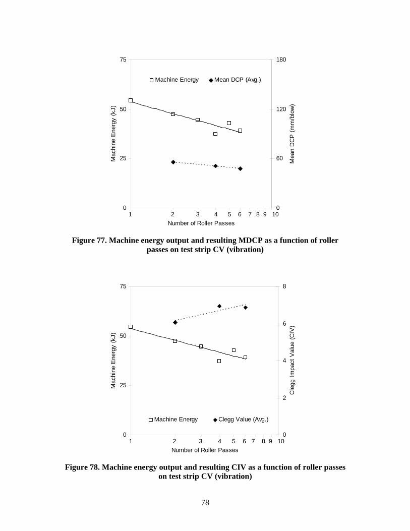
78

0

25

50

75


Mac

hine

Ene

rgy

(kJ)

0

60

120

180

Mea

n D

CP

(mm

/blo

w)


2 3 4 5 6 7 8 9 101


passes on test strip CV (vibration)

0

25

50

75


Mac

hine

Ene

rgy

(kJ)

0

2

4

6

8C

legg

Impa

ct V

alue

(CIV

)

Machine Energy Clegg Value (Avg.)

2 3 4 5 6 7 8 9 101


on test strip CV (vibration)

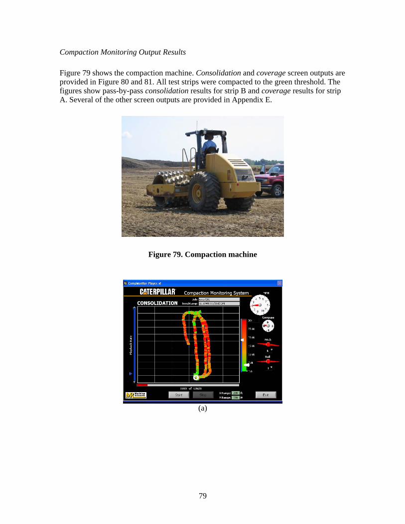
79


Figure 79 shows the compaction machine. Consolidation and coverage screen outputs are provided in Figure 80 and 81. All test strips were compacted to the green threshold. The figures show pass-by-pass consolidation results for strip B and coverage results for strip A. Several of the other screen outputs are provided in Appendix E.

Figure 79. Compaction machine

(a)

80

(b)

(c)

(d)

81

(e)

(f)

(g)

82

(h)

Figure 80. Monitor output for machine energy after 1-8 roller passes (a – h) on test strip B at W. Des Moines project site

(a)

83

(b)

(c)

(d)

Figure 81. Monitor output for machine coverage after 1-4 roller passes (a – d) on test strip A at W. Des Moines project site

84

Exploratory Study of Compaction Monitoring Output

Trend of Engine Power versus Number of Passes

Similar trends as observed in project no. 2 (i.e., reduced machine power with successive roller passes), can be observed in the machine power value box plots for test strip B (refer to Figure 82). Test strip B was on relatively flat ground. For Test strip A, where a 1:15 slope exists, the net power shows a similar pattern as the gross power (Figure 83). This suggests that the additional power required for driving uphill may not be adequately accounted for in determining the net power. Thus, the net power values may need further refinement to correctly reflect the mechanical property change in the soil being compacted.

Figure 82. Box plots for engine powers on level test strips

85

Figure 83. Box plots for engine powers when driving up and down slope, alternately

General Trend of Soil Properties versus Number of Passes

Soil mechanical properties were measured after one or two passes. Box plots and scatter plots show the expected trends in the soil properties as the number of passes increases. As shown in Figure 84, mean dry density and Clegg impact values shows an upward trend as the number of passes increases, while the MDCP values showed a downward trend, as anticipated.

86

Figure 84. Box plots of measured soil properties for third field test

However, large variations can be observed in certain soil properties at certain passes. Possible reasons for this are the inherent variability of the soil and errors in the measurement method. To reduce variation, the test points were selected in the same location for each round of measurements.

Regression Analysis

Regression analyses for test strips A and B were conducted to examine relationships between last pass power values and soil property measurements at selected test points. Based on the distance between test points, a unit section length of about 5 meters (16 ft) was used for test strip A, and a unit section length of about 3.5 m (12 ft) was used for test strip B. Soil properties measured after pass 8 in test strip B were not used in the regression analysis because the vibration was turned on only after pass 7. The impact of vibration is not discussed in the regression analysis because of the limited data set.

The same regression models were used as in previous field tests:

• Model A: Dry Density (DD) = Power (Net Power, or Gross Power) • Model B: DD = Log (Power) • Model C: DD = Log(Power) + Moisture Content (MC) • Model D: CIV = Power

87

• Model E: CIV = Log(Power) + MC • Model F: CIV = Log(Power) + MC • Model F: MDCP = Power • Model G: MDCP = Log(Power) • Model H: MDCP = Log(Power) + MC

Table 17 shows R2 values for regression models for test strips A and B. The R2 for models with GP using data from test strip A are low because of the up-hill and down-hill influences. Unfortunately, the net power did not significantly improve the regression coefficients. This is expected as the net power values did not demonstrate the desired trend in the box plots (Figure 82).

For test strip B, the gross power shows weak correlations to dry density values, CIV, and MDCP index. The net power shows improved correlations with dry density and CIV, but not DCP.

Table 17. R2 values for different regression models for test strips A and B

Test Strip A Test Strip B Models GP NP GP NP

DD = Power 0.0017 0.1070 0.2576 0.4552 DD = log(Power) 0.0001 0.0974 0.2673 0.5276 DD = MC + log(Power) 0.1120 0.2518 0.4188 0.5405 CIV = Power 0.0108 0.0020 0.1013 0.1906 CIV = log(Power) 0.0308 0.0025 0.0969 0.2128 CIV = MC + log(Power) 0.1722 0.1656 0.1880 0.2295 MDCP = Power 0.0177 0.0024 0.0069 0.0268 MDCP = log(Power) 0.0430 0.0121 0.0037 0.0301 MDCP = MC + log(Power) 0.0985 0.0984 0.0723 0.0694

The R2 value for a regression model represents the portion of variation (errors) in the dependent variable that can be explained by the independent variables. The regression results show that large portions of the errors have not been explained. It would be interesting to study the possible sources of errors with the hope that some of them can be eliminated or reduced in future tests. Some possible sources for errors in the regression models are described below.

• Soil property and power value matching method. The engine output at a certain point should be jointly determined by the soil properties at points where the compactor interacts with the soil, which should be the soil beneath the drum and wheels (refer to Figure 85). The current approach matches the power values with test points directly under the GPS receiver. Thus, the difference between the soil properties below the GPS unit and the weighted average of soil properties below the drum and the wheel will bring some errors to the regression model. To reduce this error, the test point selection method illustrated in Figure 85 is suggested.

88

Figure 85. Suggested test point settings to improve R2

• Measurement error of engine power values. Detailed information is not available regarding the accuracy of the measurement error of engine power values. Analysis results shown above have demonstrated that the net power values still need further improvement. Missing power values clearly exist, and errors in the GPS signals can also misappropriate power point values to a different unit section, thus potentially matching them to another soil property value.

• Soil property measurement error. Accurate in situ soil property measurement could have been an issue with the third field test since soil properties were collected in the exact same location each time. One solution to lower the errors from this source is to use different test points for each round of measurement of soil properties.

Key Findings and Recommendations – Project No. 3

Four test strips were compacted and tested in this third field test. A 1:15 slope exists for test strip A. To test the performance of the compaction monitoring system under sloped sited conditions, the compactor ran up-hill and down-hill alternatively. In test strip B, soil properties were measured after every one or two passes to study the relationship between soil properties and number of passes. Box plots for net power of test strip A shows that the additional power required for running up-hill is not correctly removed from the net power. Regression results using data from test strip A also confirm that under sloped conditions, the net power is not a good indicator of soil mechanical properties. Box plots for soil properties using data from test strip B demonstrate the expected trends. The regression results show that significant correlations exist between engine power values, dry density, and CIV. However, correlation between power values and MDCP values was very weak.

Two test points on wheel path

One test point on drum path

GPS receiver and location of power points

Driving direction

Test point location for current approach

89

Three possible sources of errors in the regression analysis were discussed. The following recommendations were made to reduce errors in future tests:

• Use the test point selection and power and test point matching method illustrated in Figure 85.

• Use different test point locations for each round of soil property measurement.

90

SUMMARY AND CONCLUSIONS

Measuring soil compaction during earthwork construction operations has been a key element to ensure adequate performance. Current state-of-practice relies primarily on process control (lift thickness and number of passes) and end-result spot tests. This process has several described disadvantages. To improve upon the traditional approach of spot tests, Caterpillar, Inc. (CAT), has been developing compaction monitoring technology for determining real-time compaction results with 100% test coverage. A significant advantage of this system is that measurements are output to a computer screen in the cab of the roller in real time to allow the operator to identify areas of poor compaction and make necessary rolling pattern changes. These recent developments will completely change the future of earthwork construction.

The basic premise of determining soil compaction from changes in equipment response is that mechanical energy to power the roller relates to the physical properties of the material being compacted. Laboratory compaction and strength tests show that correlating dry unit weight to the logarithm of compaction energy results in R2 values of 0.8 and that, by including water content in the multiple regression analyses, strength and stiffness can be predicted with R2 values of 0.9 and 0.6, respectively. These behavior modes set the stage for the field pilot tests.

To determine relationships between machine energy from the compaction monitoring system and various field measurements (density, DCP, and CIV), multiple linear regression analyses were also performed. The R2 of these models indicate that compaction energy accounts for more variation in dry unit weight than DCP index or Clegg impact values. Including water content in the regression analysis greatly improves the R2 models for DCP index and Clegg hammer, indicating the importance of water content on strength and stiffness.

The results of this study show that it is possible to evaluate soil compaction with relatively good accuracy using machine energy as an indicator, with the advantage of 100% coverage with results in real time. Additional field trials are necessary, however, to expand the range of correlations to other soil types, different roller configurations, roller speeds, lift thicknesses, and water contents. Further, with increased use of this technology, new QC/QA guidelines will need to be developed with a framework in statistical analysis to interpret the results. Recommendations for testing and analysis are described for Phase II in the next section of this report.

91

RECOMMENDATIONS Results from Phase I revealed that the Caterpillar compaction monitoring method has a high level of promise for use as a QC/QA tool but that additional testing is necessary in order to prove its validity under a wide range of field conditions. The Phase II work plan involves establishing a Technical Advisor Committee, developing a better understanding of the algorithms used, performing further testing in a controlled environment, testing on project sites in the Midwest, and developing QC/QA procedures, as described in more detail below.

Develop Better Understanding of Algorithms

The ISU research team needs to be able to better understand the algorithms used in the Caterpillar compaction monitoring method in order to better explain the results obtained and help develop more effective future experiments. Some of the important issues are the following:

• How net power is derived from gross power.

• How slope and machine losses are taken into account.

• Where the power values are located relative to the drum and wheels. Initially, power values were located in the middle of the compactor. Now, we understand that these values are located under the front drum. Providing some power values under the tires may need to be considered as well since compaction is occurring there too, as was shown by the difference in dry density for samples taken in and out of the wheel path.

• How the program addresses outlier data or smoothes the data. By understanding these and other issues, the ISU research team will be able to help Caterpillar refine its approach and come up with more consistent results.

Perform Controlled Experiments

Once there is a better understanding of the algorithms used in the Caterpillar compaction monitoring technology and further enhancements to the system are made, additional controlled experiments need to be performed prior to full-scale field testing. These experiments should investigate the effects of varying the soil type, lift thickness, moisture content, slope, and direction. Testing could be accomplished over a concentrated period of time at the Edwards facility or CAT Proving Grounds. A proposed testing matrix is shown in Table 18. This is a suggested work structure, but is by no means the final plan. Each test will need to be carefully considered as strategic to proving this technology. The purpose of these tests is to determine the robustness of the system under many different conditions.

92

Table 18. Proposed test plan for Phase II controlled experiments

Soil Type Moisture Content

(Relative to Optimum) Loose Lift Thickness Slope Direction

Test No. SC CL CH Dry Optimal Wet 6” 8” 10”

Down/Up Level Forward Reverse

1 x x x x x x x 2 x x x x x x x 3 x x x x x x x 4 x x x x x x x 5 x x x x x x x 6 x x x x x x x 7 x x x x x x x

These results would need to be compared to in situ test measurements, including water content, density, strength, and stiffness. Depending on the results obtained, additional adjustments to the compaction technology may be required. The research team will make every effort to standardize the field and laboratory testing methods so as to eliminate this potential source of error.

Field Testing

Field testing of the Caterpillar compaction monitoring system will be conducted on actual sites located in three or four Midwest states, one of them being Iowa. The sites will be selected based on input from the Iowa DOT, FHWA, Caterpillar, and the Technical Advisory Committee. The research team will try to select sites that have different characteristics in terms of soil type and terrain. The purpose of the field tests will be to evaluate the compaction monitoring technology under actual field conditions and a wider range of soil types. The field projects also provide the opportunity to demonstrate the technology to contractors and state agencies.

Develop QC/QA Guidelines

Based on results from these new field tests, develop a set of QC/QA guidelines for earthwork construction. The specifications are likely to be divided into method versus end-result specifications. The method specification will consider process control operations, including the number of passes of the roller and lift thickness. The end-result specification will likely involve test strip construction and validation with spot tests. Because the compaction monitoring system provides 100% test coverage, statistic procedures need to be developed to evaluate variability of data sets. Further, it is possible that incentive type specifications (i.e., owners pay based on achieved quality) could be developed similar to the paving industry.

93

Investigate Transferability to Asphalt Pavement

The initial concept considered the use of the Caterpillar compaction monitoring technology for both earthwork and asphalt compaction. All testing to date has been performed on soil. This final task will allow the research team to investigate how effective this approach will be on hot mix asphalt pavement. The ISU research team could work with a local contractor or through Caterpillar to conduct tests on different asphalt mixes. However, at this time, it is anticipated that the major research effort/scope for Phase II will continue to focus on soil compaction.

94

REFERENCES Anderegg, R. and K. Kaufmann. 2004. “Intelligent compaction with vibratory rollers.”

Transportation Research Board Annual Meeting CD-ROM, Washington, DC. Barden, L. and G. R. Sides. 1970. “Engineering behavior and structure of compacted

clay,” Journal of he Soil Mechanics and Foundations Division, ASCE, Vol. 96, No. SM4, pp. 1171.

Bekker, M. G. 1969. Introduction to Terrain-Vehicle Systems. The University of Michigan Press: Ann Arbor, Mich.

Bekker, M. G. 1956. Theory of Land Locomotion. University of Michigan Press, Ann Arbor, Mich. (2nd edition, 1962).

Bell, J.R. 1977. “Compaction Energy Relationships of Cohesive Soils.” Transportation Research Record, No. 641, p. 29-34.

Chambers, John, et al. 1983. Graphical Methods for Data Analysis, Wadsworth. Forssblad, L. 1980. “Compaction meter on vibrating rollers for improved compaction

control.” Proceedings of International Conference on Compaction, Vol. II, Paris, p. 541-546.

Froumentin, M., F. Peyret, and Y. Marineau. 1997. “GPS helps compactor operator.” Revue Generale des Routes et Des Aerodromes, Paris, pp. 1-8.

Froumentin, M., F. Peyret, and Y. Martineau. (1997). “GPS Helps Compactor Operator.” Revue Generale des Routes et de aerodromes.

Hilf, J. W. 1956. “An Investigation of Pore-Water Pressure in Compacted Cohesive Soils,” Technical Memorandum 654, U.S. Department of he Interior, Bureau of Reclamation, Denver, Colorado.

Hilf, J. W. 1991. “Compacted Fill,” in Fang, Hsai-Yang, Foundation Engineering Handbook. 2nd Edition, VanNostrand Reinhold, New York.

Hogentogler, C. A. 1936. “Essentials of soil compaction,” Proc. of the Highway Research Board, National Research Council, Washington, D.C., pp. 309-316.

Holtz, R.D. and W.D. Kovacs. 1981. An Introduction to Geotechnical Engineering. Prentice Hall, Englewood Cliffs, NJ.

Hoover, J.M. 1985. In situ Stability of Smooth-Drum Vibratory Compacted Soils with Bomag Terrameter. Final Report ERI Project 1722. Engineering Research Institute, Iowa State Univ., Ames, Iowa, 64 pp.

Johnson, A. W., and J. R. Sallberg. 1960. “Factors That Influence Field Compaction of Soil,” Highway Research Board, Bulletin No. 272.

Lambe, T.W. 1958a. “The structure of compacted clay.” Journal of the Soil Mechanics and Foundation Division, ASCE, Vol. 84, No. SM2, pp. 1654-1 to 34.

Lambe, T.W. 1958b. “The engineering behavior of compacted clay.” Journal of the Soil Mechanics and Foundation Division, ASCE, Vol. 84, No. SM2, pp. 1655-1 to 35.

95

Lambe, T. W. 1960. “The character and identification of expansive soils, soil PVC meter,” Federal Housing Administration, Technical Studies Program, FHA 70 1.

Liston, R. A., L. A. Martin. 1966. “Multipass Behavior of a Rigid Wheel,” Proc. Sec. Int. Conf. on Terrain-Vehicle Systems, Quebec City, Que., Toronto Univ. Press, Toronto.

Morin, M. 1865. Second Memoire sur le triage des voitures et sur les effets destructeurs, qu’elles exercent sur les routes. (Second memorandum on hauling carriages), Comptes Rendus Acad. De Science, Vol. X, pp. 101-4.

Olsen, R. E. 1963. “Effective stress theory of soil compaction,” Journal of the Soil Mechanics and Foundation Division, ASCE, Vol. 89, No. SM2, pp. 27-45.

Proctor, R. R. 1933. “The design and construction of roller earth dams,” Engineering News Record III, August 31, September 7,21, and 28

Rhind, D. 2001. Geographic Information System and Science, John Wiley & Sons, Inc., Hoboken, NJ.

Sandström, A.J. and C.B. Pettersson. 2004. “Intelligent Systems for QA/QC in Soil Compaction.” Presented, Transportation Research Board. 83rd Meeting, Washington D.C., January 11-15.

Seed, H.B. and C.K. Chan. 1959. “Structure and strength characteristics of compacted clays.” Journal of the Soil Mechanics and Foundation Division, ASCE, Vol. 85, No. SM5, pp. 87-128.

Selig, E.T. 1966. “Variability of Compacted Soils.” National Conference on Statistical Quality Control Methodology in Highway and Airfield Construction, Nov. 1966, pp. 181-213.

Shuring, D. J. 1966. “The Energy Loss of a Wheel,” Proc. Sec. Int. Conf. on Terrain-Vehicle Systems, Quebec City, Que., Toronto Univ. Press, Toronto.

Spangler, M.G. and R.L. Handy. 1982. Soil Engineering. Fourth Edition, Harper and Row Publishers, New York.

Thurner, H.F. and A.J. Sandström. 1980. “A New Device for Instant Compaction Control.” Proceedings of International Conference on Compaction, Vol. II, Paris, p. 611-614.

Thurner, H.F., and A.J. Sandström. 2000. “Continuous Compaction Control, CCC.” Compaction of Soils and Granular Materials. Modeling and Properties of Compacted Materials, Paris, p. 237-245.

WES. 1964. “Trafficability Tests with the Marsh Screw Amphibian,” Waterways Experiment Station No. 3-641, Vicksburg, Miss.

White, D.J., K.L. Bergeson, and C.T. Jahren. 2002. “Embankment Quality – Phase III,”

Final Report, Iowa DOT Project TR-401, CTRE Project 97-8, June 2002. Won-Seok, D. A.A. Oloufa, and H.R. Thomas. 1999. “Evaluation of global positioning

system devices for a quality control system for compaction operations.” Transportation Research Record 1675, pp. 67-74.

96

APPENDIX A: LABORATORY TEST RESULTS – PROJECT NO. 1

97

18

19

20

21

22

23

4.0 6.0 8.0 10.0 12.0Moisture Content, (%)

Dry

Uni

t Wei

ght,

(kN

/m3 )

355

592

987

2693

ZAV



Figure A1. Dry unit weight results from unconfined compression tests for various compaction energies (Edwards till)

98

0

300

600

900

0.00 0.02 0.04 0.06 0.08Strain (mm/mm)

Stre

ss (k

Pa)

355 at 6.0592 at 5.5987 at 5.22693 at 5.0

Compaction Energy (kJ/m3)at Moisture Content (%)

Figure A2. Unconfined compression results for various compaction energies at

approximately 5.0% moisture content (PPG till)

0

100

200

300

400

500

600

0.00 0.01 0.02 0.03 0.04 0.05 0.06 0.07Strain (mm/mm)

Stre

ss (k

Pa)

355 at 6.7592 at 6.8987 at 6.82693 at 7.0




99

0

100

200

300

0.00 0.02 0.04 0.06 0.08 0.10 0.12 0.14Strain (mm/mm)

Stre

ss (k

Pa)

355 at 7.7592 at 7.7987 at 8.42693 at 8.1




0

30

60

90

120

150

0.00 0.05 0.10 0.15 0.20Strain (mm/mm)

Stre

ss (k

Pa)

355 at 9.2592 at 9.4987 at 10.1




100

0

20

40

60

80

100

120

140

160

180

200

0.00 0.05 0.10 0.15 0.20Strain (mm/mm)

Stre

ss (k

Pa)

66.77.79.2


Figure A6. Unconfined compression results delivered with a compaction energy of

355 kJ/m3 at various moisture contents (PPG till)

0

70

140

210

280

350

0.00 0.02 0.04 0.06 0.08 0.10 0.12 0.14Strain (mm/mm)

Stre

ss (k

Pa)

5.56.87.79.4




101

0

100

200

300

400

500

0.00 0.05 0.10 0.15 0.20Strain (mm/mm)

Stre

ss (k

Pa)

5.26.88.410.1




0

300

600

900

0.00 0.02 0.04 0.06 0.08 0.10 0.12Strain (mm/mm)

Stre

ss (k

Pa)

578.1




102

APPENDIX B: STATISTICAL ANALYSIS RESULTS– PROJECT NO. 1

103

Outline of Statistical Analysis – Project No. 1

I. Soil Property – Engine Power Relationship A. Paired Scatter Plots

B. Regression Results II. Measure Power Values A. Box Plots B. Summary Statistics III. Measure Soil Properties A. Box Plots B. Summary Statistics

I. Soil Property – Engine Power Relationship

A. Paired Scatter Plots

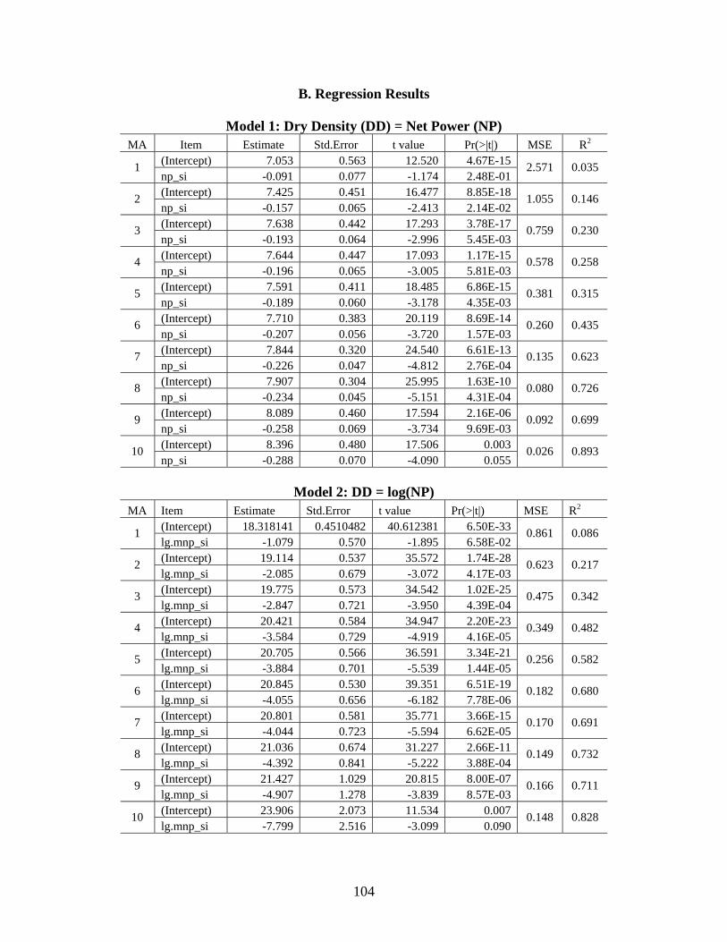
104

B. Regression Results

Model 1: Dry Density (DD) = Net Power (NP) MA Item Estimate Std.Error t value Pr(>|t|) MSE R2

(Intercept) 7.053 0.563 12.520 4.67E-15 1 np_si -0.091 0.077 -1.174 2.48E-01

2.571 0.035


1.055 0.146


0.759 0.230


0.578 0.258


0.381 0.315


0.260 0.435


0.135 0.623


0.080 0.726


0.092 0.699

(Intercept) 8.396 0.480 17.506 0.003 10 np_si -0.288 0.070 -4.090 0.055

0.026 0.893

Model 2: DD = log(NP)

MA Item Estimate Std.Error t value Pr(>|t|) MSE R2 (Intercept) 18.318141 0.4510482 40.612381 6.50E-33 1 lg.mnp_si -1.079 0.570 -1.895 6.58E-02

0.861 0.086

(Intercept) 19.114 0.537 35.572 1.74E-28 2 lg.mnp_si -2.085 0.679 -3.072 4.17E-03

0.623 0.217


0.475 0.342


0.349 0.482


0.256 0.582


0.182 0.680


0.170 0.691


0.149 0.732


0.166 0.711

(Intercept) 23.906 2.073 11.534 0.007 10 lg.mnp_si -7.799 2.516 -3.099 0.090

0.148 0.828

105

Model 3: DD = log(NP) + MC MA Item Estimate Std.Error t value Pr(>|t|) MSE R2

(Intercept) 19.557 1.267 15.433 1.06E-17 mc -0.143 0.136 -1.046 3.02E-01 1 lg.mnp_si -1.013 0.573 -1.769 8.51E-02

0.8592

0.1125


0.6288

0.2326


0.4913

0.3422

(Intercept) 20.354 1.355 15.020 5.09E-14 mc 0.009 0.155 0.055 9.56E-01 4 lg.mnp_si -3.596 0.776 -4.635 9.60E-05

0.3627

0.4821


0.2653 0.587


0.1693

0.7181


0.1394

0.7649


0.1197

0.8056

(Intercept) 17.618 2.212 7.964 0.001 mc 0.490 0.262 1.871 0.120 9 lg.mnp_si -5.686 1.152 -4.937 0.004

0.117 0.8298


0.0075

0.9956

106

Model 4: Clegg Impact Value (CIV) = NP MA Item Estimate Std.Error t value Pr(>|t|) MSE R2


2.571 0.035


1.055 0.146


0.759 0.230


0.578 0.258


0.381 0.315


0.260 0.435


0.135 0.623


0.080 0.726


0.092 0.699

(Intercept) 8.396 0.480 17.506 0.003 10 np_si -0.288 0.070 -4.090 0.055

0.026 0.893

Model 5: CIV = log(NP)

MA Item Estimate Std.Error t value Pr(>|t|) MSE R2 (Intercept) 7.368 0.778 9.471 1.51E-11 1 lg.mnp_si -1.210 0.983 -1.231 2.26E-01

2.562 0.038


1.016 0.178


0.749 0.241


0.581 0.254


0.382 0.314


0.272 0.408


0.150 0.583


0.093 0.685


0.105 0.655


0.027 0.890

107

Model 6: CIV = log(NP) + MC MA Item Estimate Std.Error t value Pr(>|t|) MSE R2


2.311 0.155


0.969 0.238


0.737 0.278


0.577 0.287


0.391 0.329


0.288 0.408


0.161 0.585

(Intercept) 9.291 1.548 6.003 2.02E-04 mc -0.055 0.178 -0.309 0.764 8 lg.mnp_si -3.035 0.724 -4.192 0.002

0.102 0.688

(Intercept) 9.780 2.279 4.291 0.008 mc -0.079 0.270 -0.294 0.781 9 lg.mnp_si -3.315 1.187 -2.794 0.038

0.124 0.661


0.015 0.969

108

II. Measured Power Values

A. Box Plots

B. Summary Statistics for Net Power by Pass:

Section 2 Section 3

Pass 1 Pass 2 Pass 1 Pass 2 Pass 3 Means (KW): 12.558 7.285 11.563 5.408 6.231 Std Devs (KW) 4.470 4.885 4.834 5.881 4.504 C.O.V. (%) 36 67 42 109 72 Maxs (KW): 21.801 25.854 19.744 35.391 20.269 Medians (KW): 13.617 6.629 12.255 3.574 6.160 Mins (KW): 0.826 0.017 0.115 0.002 0.034

109

III. Measured Soil Properties A. Box Plots

B. Summary Statistics

Dry Density Section 1 Section 2 Section 3 Means (KW): 16.274 16.990 18.030 Std Devs (KW) 0.738 0.643 0.950 C.O.V. (%) 4.5 3.8 5.3 Maxs (KW): 18.045 18.226 20.002 Medians (KW): 16.207 17.001 17.712 Mins (KW): 14.895 15.657 16.474

Moisture Content

Section 1 Section 2 Section 3 Means (KW): 8.560 8.740 9.333 Std Devs (KW) 0.832 0.968 1.158 C.O.V. (%) 9.7 11.1 12.4 Maxs (KW): 10.000 10.750 11.350 Medians (KW): 8.650 8.575 9.200 Mins (KW): 7.000 7.500 7.850

Clegg Impact Value

Section 1 Section 2 Section 3 Means (KW): 6.635 6.205 6.720 Std Devs (KW) 2.729 1.644 1.577 C.O.V. (%) 41 27 24 Maxs (KW): 16.000 10.300 10.700 Medians (KW): 6.000 5.750 6.350 Mins (KW): 3.800 4.200 4.600

110

APPENDIX C: LABORATORY AND FIELD TEST RESULTS – PROJECT NO. 2

111

16

17

18

19

20

21

22

4.0 8.0 12.0 16.0 20.0

Moisture Content, (%)

Dry

Uni

t Wei

ght,

(kN

/m3 )

35559298716432693ZAV curve



Figure C1. Dry unit weight results from unconfined compression tests for various

compaction energies (Edwards till)

112

0

200

400

600

800

1000

0.000 0.005 0.010 0.015 0.020 0.025Strain (mm/mm)

Stre

ss (k

Pa)

355 at 5.4 592 at 5.5987 at 5.41643 at 5.12693 at 5.1

Compaction Energy (kJ/m3) at Mosture Content (%)

Figure C2. Unconfined compression results for various compaction energies at

approximately 5.0% moisture content (Edwards till)

0

300

600

900

1200

0.00 0.01 0.02 0.03 0.04 0.05

Strain (mm/mm)

Stre

ss (k

Pa)

355 at 8.5592 at 8.9987 at 8.71643 at 8.52693 at 8.3

Compaction Energy (kJ/m3)at MoistureContent (%)



113

0

150

300

450

600

750

900

0.00 0.05 0.10 0.15Strain (mm/mm)

Stre

ss (k

Pa)

355 at 11

592 at 11.2

987 at 11.2

1643 at 10.7

1643 at 12.4

2693 at 10.8




0

70

140

210

280

350

0.00 0.05 0.10 0.15 0.20Strain (mm/mm)

Stre

ss (k

Pa)

355 at 13.8%12375 at 13.7%20624 at 14.1%56248 at 13.8%




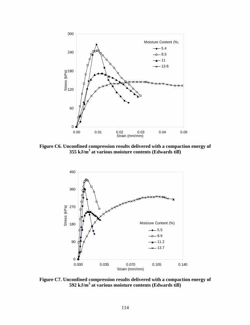
114

0

60

120

180

240

300

0.00 0.01 0.02 0.03 0.04 0.05Strain (mm/mm)

Stre

ss (k

Pa)

5.48.51113.8


Figure C6. Unconfined compression results delivered with a compaction energy of

355 kJ/m3 at various moisture contents (Edwards till)

0

90

180

270

360

450

0.000 0.035 0.070 0.105 0.140Strain (mm/mm)

Stre

ss (k

Pa)

5.58.911.213.7




115

0

100

200

300

400

500

600

0.00 0.05 0.10 0.15 0.20Strain (mm/mm)

Stre

ss (k

Pa)

5.48.711.214.1




0

300

600

900

0.000 0.035 0.070 0.105 0.140Strain (mm/mm)

Stre

ss (k

Pa)

4.55.18.510.712.4




116

0

220

440

660

880

1100

0.00 0.06 0.12 0.18Strain (mm/mm)

Stre

ss (k

Pa)

5.18.310.813.8




117

Table C1. Summary of test results for test strip A

Nuclear Field Samples TDR Measurements

Test Point

X-coord.

Y-coord.

Water content

(%)

Dry Unit Weight (pcf)

Water content (%)


Clegg Impact Value

MDCP Index (mm/ blow)

Test in wheel path?

UCS Estimated from Pocket Penetrometer

(tsf)

Loose lift (in)

Number of

Roller Passes

Theta-v std

cal. Theta-v Theta V

1A 44 27 9.0 105.4 8.3 115.7 17.2 12 Y 4.5 12 6 23.1 15.12 15.39 2A 55 26 8.0 106.7 8.5 ⎯ 16.7 17 Y ⎯ 12 6 22.2 13.67 0.00 3A 57 32 12.9 99.8 8.2 ⎯ 10.5 37 Y ⎯ 12 6 29.9 20.62 0.00 4A 67 29 10.8 98.8 9.3 113.1 15.4 20 N 4.5 12 6 25.3 17.10 16.86 5A 71 27 9.7 106.2 8.5 ⎯ 14.9 15 N ⎯ 12 6 23.7 16.42 0.00 6A 79 29 9.4 102.4 9.1 ⎯ 13.7 28 N ⎯ 12 6 22.4 15.42 0.00 7A 82 29 9.5 100.0 8.6 ⎯ 11.8 28 N ⎯ 12 6 23.7 15.22 0.00 8A 85 29 10.0 101.8 9.3 108.2 10.6 32 N 4.5 12 6 21.8 16.31 16.13 9A 97 25 7.2 108.1 7.8 ⎯ 11.7 19 Y ⎯ 12 6 20.9 12.47 0.00

10A 97 29 8.9 102.0 8.5 ⎯ 7.5 31 N ⎯ 12 6 21.4 14.46 0.00

Table C2. Summary of test results for test strip B


Test Point

X-coord.

Y-coord.

Water content

(%)

Dry Unit Weight

(pcf)

Water content (%)

Dry Unit Weight

(pcf)

Clegg Impact Value


Test in wheel path?

UCS Estimated

from Pocket Penetrometer

(tsf)

Loose lift (in)

Number of

Roller Passes

Theta-v std


1B 47 35 14.3 103.2 12.9 ⎯ 10.5 45 Y ⎯- 16 6 34.8 23.57 0.00 2B 48 38 13.8 101.8 13.2 112.2 7.1 52 N 3.8 16 6 26.6 22.51 23.73 3B 60 38 13.4 100.1 12.7 ⎯ 6.8 50 N ⎯ 16 6 30.1 21.50 0.00 4B 65 36 14.5 101.7 12.4 113.1 7.5 49 N 4.5 16 6 33.4 23.55 22.54 5B 67 39 13.6 101.2 12.5 ⎯ 11.5 44 Y ⎯ 16 6 34.7 21.96 0.00 6B 75 39 13.5 102.7 12.7 ⎯ 9.1 50 Y ⎯ 16 6 32.1 22.22 0.00 7B 82 40 15.3 104.0 12.8 ⎯ 8.1 48 Y ⎯ 16 6 35.1 25.40 0.00 8B 86 36 12.6 101.0 12.1 ⎯ 11.2 43 N ⎯ 16 6 29.5 20.39 0.00 9B 92 37 13.5 99.7 12.2 101.8 8.3 49 N 3.6 16 6 30.6 21.56 19.90

10B 96 35 11.4 101.7 11.4 ⎯ 9.7 39 N ⎯ 16 6 28.8 18.49 0.00

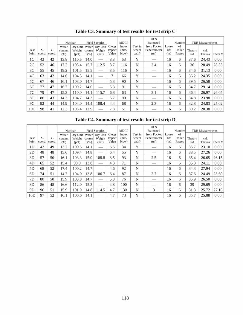
118

Table C3. Summary of test results for test strip C


Test Point

X-coord.

Y-coord.

Water content

(%)

Dry Unit Weight

(pcf)

Water content (%)

Dry Unit Weight

(pcf)

Clegg Impact Value


Test in wheel path?

UCS Estimated


(tsf)

Loose lift (in)

Number of

Roller Passes

Theta-v std


1C 42 42 13.8 110.5 14.0 ⎯ 8.3 53 Y ⎯ 16 6 37.6 24.43 0.00 2C 52 46 17.2 103.4 15.7 112.5 3.7 116 N 2.4 16 6 36 28.49 28.333C 55 45 19.2 101.5 15.5 ⎯ 3.5 116 N ⎯ 16 6 34.6 31.13 0.00 4C 63 42 14.6 104.5 14.1 ⎯ 7 66 Y ⎯ 16 6 36.2 24.35 0.00 5C 67 46 16.1 103.0 14.7 ⎯ 5.3 90 N ⎯ 16 6 39.5 26.58 0.00 6C 72 47 16.7 109.2 14.0 ⎯ 5.3 91 Y ⎯ 16 6 34.7 29.14 0.00 7C 79 47 15.3 110.0 14.1 115.7 6.8 63 Y 3.1 16 6 36.4 26.97 26.058C 86 43 14.3 104.7 14.3 ⎯ 5.7 90 N ⎯ 16 6 34.8 23.98 0.00 9C 92 44 14.9 104.0 14.4 108.4 4.4 68 N 2.3 16 6 32.8 24.83 25.02

10C 98 41 12.3 103.4 12.9 ⎯ 7.3 51 N ⎯ 16 6 30.2 20.38 0.00

Table C4. Summary of test results for test strip D


Test Point

X-coord.

Y-coord.

Water content

(%)

Dry Unit Weight

(pcf)

Water content (%)

Dry Unit Weight

(pcf)

Clegg Impact Value


Test in wheel path?

UCS Estimated


(tsf)

Loose lift (in)

Number of

Roller Passes

Theta-v std


1D 42 49 13.2 109.5 14.1 ⎯ 6.5 34 Y ⎯ 16 6 35.7 23.10 0.00 2D 48 48 15.6 109.4 14.8 ⎯ 6.4 55 Y ⎯ 16 6 38.5 27.26 0.00 3D 57 50 16.1 103.3 15.0 108.8 3.5 93 N 2.5 16 6 35.4 26.65 26.154D 65 52 15.4 98.0 13.8 ⎯ 4.3 71 N ⎯ 16 6 35.8 24.11 0.00 5D 68 52 17.4 100.2 14.7 ⎯ 4.6 92 N ⎯ 16 6 34.3 27.94 0.00 6D 74 51 14.7 104.0 13.8 106.7 6.4 87 N 2.7 16 6 37.6 24.49 23.607D 80 50 15.9 103.8 14.7 ⎯ 5.3 76 N ⎯ 16 6 35.9 26.50 0.00 8D 86 48 16.6 112.0 15.3 ⎯ 4.8 100 N ⎯ 16 6 39 29.69 0.00 9D 96 51 15.9 101.0 14.8 114.5 4.7 130 N 3 16 6 31.3 25.72 27.16

10D 97 52 16.1 100.6 14.1 ⎯ 4.7 73 Y ⎯ 16 6 35.7 25.88 0.00

119

Table C5. Summary of test results for test strip E


Test Point

X-coord.

Y-coord.

Water content

(%)

Dry Unit Weight

(pcf)

Water content

(%)


Clegg Impact Value


Test in wheel path?

UCS Estimated


(tsf)

Loose lift (in)

Number of

Roller Passes

Theta-v std


1E 16 67 10.3 104.9 8.5 ---- 19.8 12 ---- ---- 10 10 ⎯ ⎯ ⎯ 2E 21 64 7.6 106.4 8.2 108.6 19 18 ---- 4.5 10 10 ⎯ ⎯ ⎯ 3E 32 66 8.4 105.7 8.3 ---- 22.7 10 ---- ---- 10 10 ⎯ ⎯ ⎯ 4E 36 68 9.3 99.8 8.4 ---- 13.4 19 ---- ---- 10 10 ⎯ ⎯ ⎯ 5E 41 63 8.9 107.9 8.3 113.5 21.7 12 ---- 4.5 10 10 ⎯ ⎯ ⎯ 6E 47 62 8.5 105.8 8.3 ---- 14.5 16 ---- ---- 10 10 ⎯ ⎯ ⎯ 7E 51 67 8.7 106.3 8.2 ---- 24.7 26 ---- ---- 10 10 ⎯ ⎯ ⎯ 8E 58 61 8.5 104.9 9.1 115.3 16.6 17 ---- 4.5 10 10 ⎯ ⎯ ⎯ 9E 64 60 9.6 106.4 8.2 ---- 19.1 16 ---- ---- 10 10 ⎯ ⎯ ⎯

10E 69 64 9.2 108.1 8.2 ---- 31.3 9 ---- ---- 10 10 ⎯ ⎯ ⎯

Table C6. Summary of test results for test strip F


Test Point

X-coord.

Y-coord.

Water content

(%)


Water content

(%)

Dry Unit Weight

(pcf)

Clegg Impact Value


Test in wheel path?

UCS Estimated


(tsf)

Loose lift (in)

Number of

Roller Passes

Theta-v std


1F 43 81 18.4 100.7 13.7 115.4 6.1 59 Y 3.8 26-28 10 ⎯ ⎯ ⎯ 2F 52 81 18.0 103.9 13.6 ⎯ 6.9 60 Y ⎯ 26-28 10 ⎯ ⎯ ⎯ 3F 60 86 15.8 108.2 14.1 ⎯ 7.5 69 Y ⎯ 26-28 10 ⎯ ⎯ ⎯ 4F 63 84 14.4 105.8 12.3 ⎯ 8 49 N ⎯ 26-28 10 ⎯ ⎯ ⎯ 5F 67 81 13.3 111.5 12.1 121.8 7.1 57 N 4.5 26-28 10 ⎯ ⎯ ⎯ 6F 72 85 17.2 107.3 15.1 ⎯ 4.6 95 Y ⎯ 26-28 10 ⎯ ⎯ ⎯ 7F 83 83 15.5 111.8 14.5 117.2 5.7 56 N 2.4 26-28 10 ⎯ ⎯ ⎯ 8F 88 82 13.1 110.3 13.5 ⎯ 7.5 47 N ⎯ 26-28 10 ⎯ ⎯ ⎯ 9F 96 81 15.5 103.1 12.5 ⎯ 8.7 54 N ⎯ 26-28 10 ⎯ ⎯ ⎯

10F 98 81 14.7 105.5 12.6 ⎯ 14.1 49 N ⎯ 26-28 10 ⎯ ⎯ ⎯

Table C7. Summary of test results for test strip G


Test Point

X-coord.

Y-coord.

Water content

(%)


Water content (%)


Clegg Impact Value


Test in wheel path?

UCS Estimated


(tsf)

Loose lift (in)


Theta-v std


1G 63 95 12.8 112.8 12.1 123.6 10.4 47 Y 4.5 26 10 ⎯ ⎯ ⎯ 2G 69 98 12.7 109.1 12.2 123.2 12.4 41 N 4.5 26 10 ⎯ ⎯ ⎯ 3G 74 97 12.7 102.4 12.0 115.6 9.2 41 N 4.5 26 10 ⎯ ⎯ ⎯ 4G 82 99 12.9 110.8 12.0 ⎯ 12.9 38 Y ⎯ 26 10 ⎯ ⎯ ⎯ 5G 88 99 13.0 111.7 11.6 ⎯ 13.1 38 Y ⎯ 26 10 ⎯ ⎯ ⎯

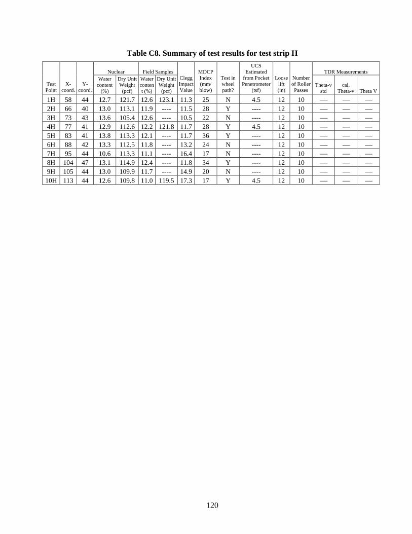
120

Table C8. Summary of test results for test strip H


Test Point

X-coord.

Y-coord.

Water content

(%)


Water content (%)


Clegg Impact Value


Test in wheel path?

UCS Estimated


(tsf)

Loose lift (in)


Theta-v std


1H 58 44 12.7 121.7 12.6 123.1 11.3 25 N 4.5 12 10 ⎯ ⎯ ⎯ 2H 66 40 13.0 113.1 11.9 ---- 11.5 28 Y ---- 12 10 ⎯ ⎯ ⎯ 3H 73 43 13.6 105.4 12.6 ---- 10.5 22 N ---- 12 10 ⎯ ⎯ ⎯ 4H 77 41 12.9 112.6 12.2 121.8 11.7 28 Y 4.5 12 10 ⎯ ⎯ ⎯ 5H 83 41 13.8 113.3 12.1 ---- 11.7 36 Y ---- 12 10 ⎯ ⎯ ⎯ 6H 88 42 13.3 112.5 11.8 ---- 13.2 24 N ---- 12 10 ⎯ ⎯ ⎯ 7H 95 44 10.6 113.3 11.1 ---- 16.4 17 N ---- 12 10 ⎯ ⎯ ⎯ 8H 104 47 13.1 114.9 12.4 ---- 11.8 34 Y ---- 12 10 ⎯ ⎯ ⎯ 9H 105 44 13.0 109.9 11.7 ---- 14.9 20 N ---- 12 10 ⎯ ⎯ ⎯

10H 113 44 12.6 109.8 11.0 119.5 17.3 17 Y 4.5 12 10 ⎯ ⎯ ⎯

121

DCP Index Test Results 1A 2A

0

5

10

15

20

25

30

35

40

1 10 100CBR

DEP

TH, i

n.0

100

200

300

400

500

600

700

800

900

10001 10 100

DEP

TH, m

m

0

5

10

15

20

25

30

35

40

1 10 100CBR

DEP

TH, i

n.

0

100

200

300

400

500

600

700

800

900

10001 10 100

DEP

TH, m

m

3A 4A

0

5

10

15

20

25

30

35

40

1 10CBR

DEP

TH, i

n.

0

100

200

300

400

500

600

700

800

900

10001 10 100

DE

PTH

, mm

0

5

10

15

20

25

30

35

40

1 10 100CBR

DEP

TH, i

n.

0

100

200

300

400

500

600

700

800

900

10001 10 100

DE

PTH

, mm

5A 6A

0

5

10

15

20

25

30

35

40

1 10 100CBR

DEP

TH, i

n.

0

100

200

300

400

500

600

700

800

900

10001 10 100

DE

PTH

, mm

0

5

10

15

20

25

30

35

40

1 10 100CBR

DEP

TH, i

n.

0

100

200

300

400

500

600

700

800

900

10001 10 100

DE

PTH

, mm

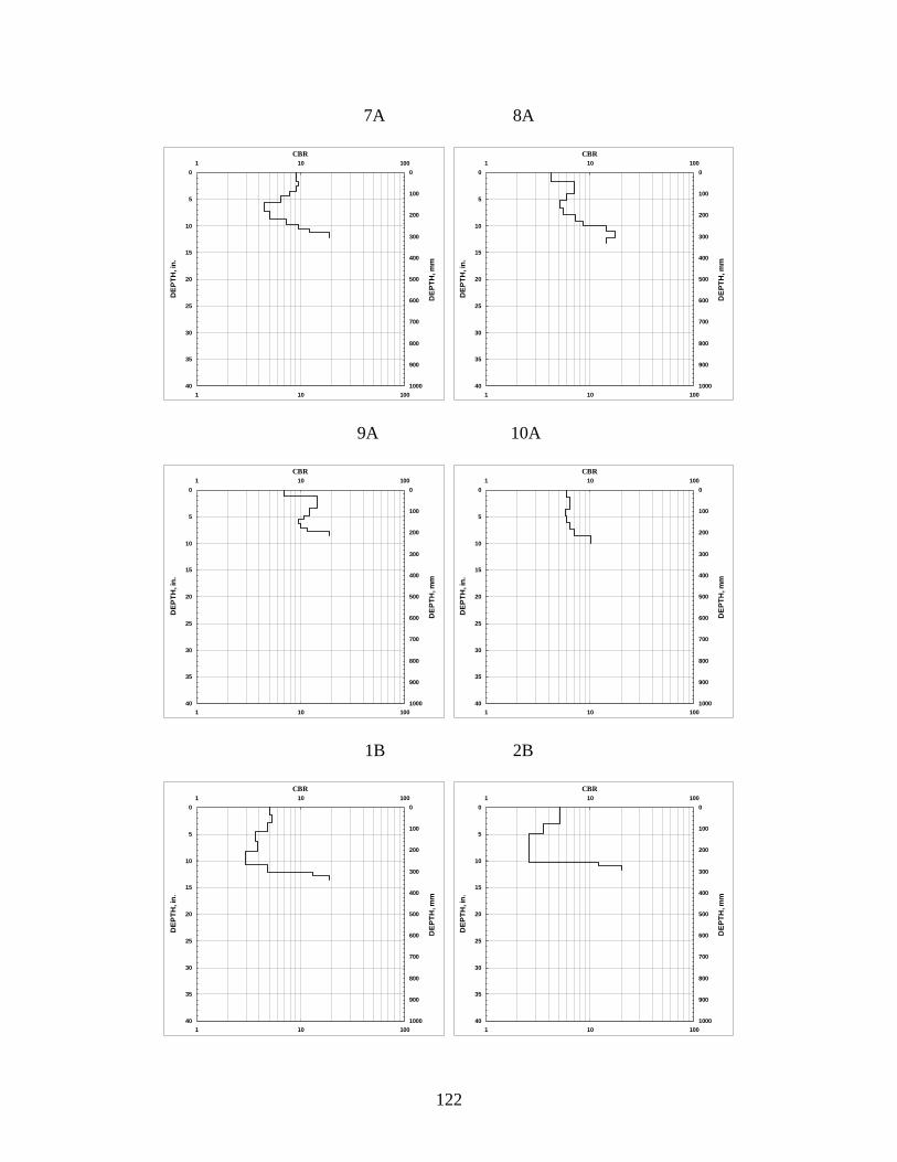
122

7A 8A

0

5

10

15

20

25

30

35

40

1 10 100CBR

DEP

TH, i

n.0

100

200

300

400

500

600

700

800

900

10001 10 100

DE

PTH

, mm

0

5

10

15

20

25

30

35

40

1 10 100CBR

DEP

TH, i

n.

0

100

200

300

400

500

600

700

800

900

10001 10 100

DE

PTH

, mm

9A 10A

0

5

10

15

20

25

30

35

40

1 10 100CBR

DEP

TH, i

n.

0

100

200

300

400

500

600

700

800

900

10001 10 100

DE

PTH

, mm

0

5

10

15

20

25

30

35

40

1 10 100CBR

DEP

TH, i

n.

0

100

200

300

400

500

600

700

800

900

10001 10 100

DE

PTH

, mm

1B 2B

0

5

10

15

20

25

30

35

40

1 10 100CBR

DEP

TH, i

n.

0

100

200

300

400

500

600

700

800

900

10001 10 100

DE

PTH

, mm

0

5

10

15

20

25

30

35

40

1 10 100CBR

DEP

TH, i

n.

0

100

200

300

400

500

600

700

800

900

10001 10 100

DE

PTH

, mm

123

3B 4B

0

5

10

15

20

25

30

35

40

1 10 100CBR

DEP

TH, i

n.0

100

200

300

400

500

600

700

800

900

10001 10 100

DE

PTH

, mm

0

5

10

15

20

25

30

35

40

1 10 100CBR

DEP

TH, i

n.

0

100

200

300

400

500

600

700

800

900

10001 10 100

DE

PTH

, mm

5B 6B

0

5

10

15

20

25

30

35

40

1 10 100CBR

DEP

TH, i

n.

0

100

200

300

400

500

600

700

800

900

10001 10 100

DE

PTH

, mm

0

5

10

15

20

25

30

35

40

1 10 100CBR

DEP

TH, i

n.

0

100

200

300

400

500

600

700

800

900

10001 10 100

DE

PTH

, mm

7B 8B

0

5

10

15

20

25

30

35

40

1 10 100CBR

DEP

TH, i

n.

0

100

200

300

400

500

600

700

800

900

10001 10 100

DE

PTH

, mm

0

5

10

15

20

25

30

35

40

1 10 100CBR

DEP

TH, i

n.

0

100

200

300

400

500

600

700

800

900

10001 10 100

DE

PTH

, mm

124

9B 10B

0

5

10

15

20

25

30

35

40

1 10 100CBR

DEP

TH, i

n.0

100

200

300

400

500

600

700

800

900

10001 10 100

DE

PTH

, mm

0

5

10

15

20

25

30

35

40

1 10 100CBR

DEP

TH, i

n.

0

100

200

300

400

500

600

700

800

900

10001 10 100

DE

PTH

, mm

1C 2C

0

5

10

15

20

25

30

35

40

1 10 100CBR

DEP

TH, i

n.

0

100

200

300

400

500

600

700

800

900

10001 10 100

DE

PTH

, mm

0

5

10

15

20

25

30

35

40

1 10 100CBR

DEP

TH, i

n.

0

100

200

300

400

500

600

700

800

900

10001 10 100

DE

PTH

, mm

3C 4C

0

5

10

15

20

25

30

35

40

1 10 100CBR

DEP

TH, i

n.

0

100

200

300

400

500

600

700

800

900

10001 10 100

DE

PTH

, mm

0

5

10

15

20

25

30

35

40

1 10 100CBR

DEP

TH, i

n.

0

100

200

300

400

500

600

700

800

900

10001 10 100

DE

PTH

, mm

125

5C 6C

0

5

10

15

20

25

30

35

40

1 10 100CBR

DEP

TH, i

n.

0

100

200

300

400

500

600

700

800

900

10001 10 100

DE

PTH

, mm

0

5

10

15

20

25

30

35

40

1 10 100CBR

DEP

TH, i

n.

0

100

200

300

400

500

600

700

800

900

10001 10 100

DE

PTH

, mm

7C 8C

0

5

10

15

20

25

30

35

40

1 10 100CBR

DEP

TH, i

n.

0

100

200

300

400

500

600

700

800

900

10001 10 100

DE

PTH

, mm

0

5

10

15

20

25

30

35

40

1 10 100CBR

DEP

TH, i

n.

0

100

200

300

400

500

600

700

800

900

10001 10 100

DE

PTH

, mm

9C 10C

0

5

10

15

20

25

30

35

40

1 10 100CBR

DEP

TH, i

n.

0

100

200

300

400

500

600

700

800

900

10001 10 100

DE

PTH

, mm

0

5

10

15

20

25

30

35

40

1 10 100CBR

DEP

TH, i

n.

0

100

200

300

400

500

600

700

800

900

10001 10 100

DE

PTH

, mm

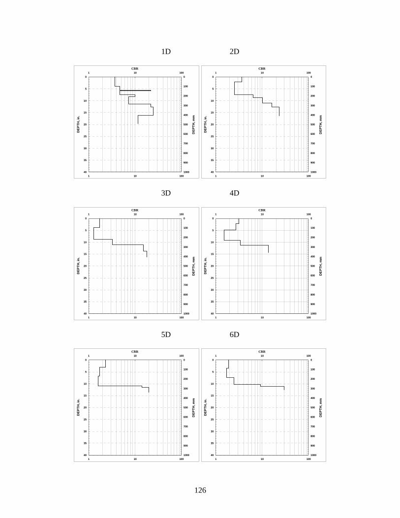
126

1D 2D

0

5

10

15

20

25

30

35

40

1 10 100CBR

DEP

TH, i

n.0

100

200

300

400

500

600

700

800

900

10001 10 100

DE

PTH

, mm

0

5

10

15

20

25

30

35

40

1 10 100CBR

DEP

TH, i

n.

0

100

200

300

400

500

600

700

800

900

10001 10 100

DE

PTH

, mm

3D 4D

0

5

10

15

20

25

30

35

40

1 10 100CBR

DEP

TH, i

n.

0

100

200

300

400

500

600

700

800

900

10001 10 100

DE

PTH

, mm

0

5

10

15

20

25

30

35

40

1 10 100CBR

DEP

TH, i

n.

0

100

200

300

400

500

600

700

800

900

10001 10 100

DE

PTH

, mm

5D 6D

0

5

10

15

20

25

30

35

40

1 10 100CBR

DEP

TH, i

n.

0

100

200

300

400

500

600

700

800

900

10001 10 100

DE

PTH

, mm

0

5

10

15

20

25

30

35

40

1 10 100CBR

DEP

TH, i

n.

0

100

200

300

400

500

600

700

800

900

10001 10 100

DE

PTH

, mm

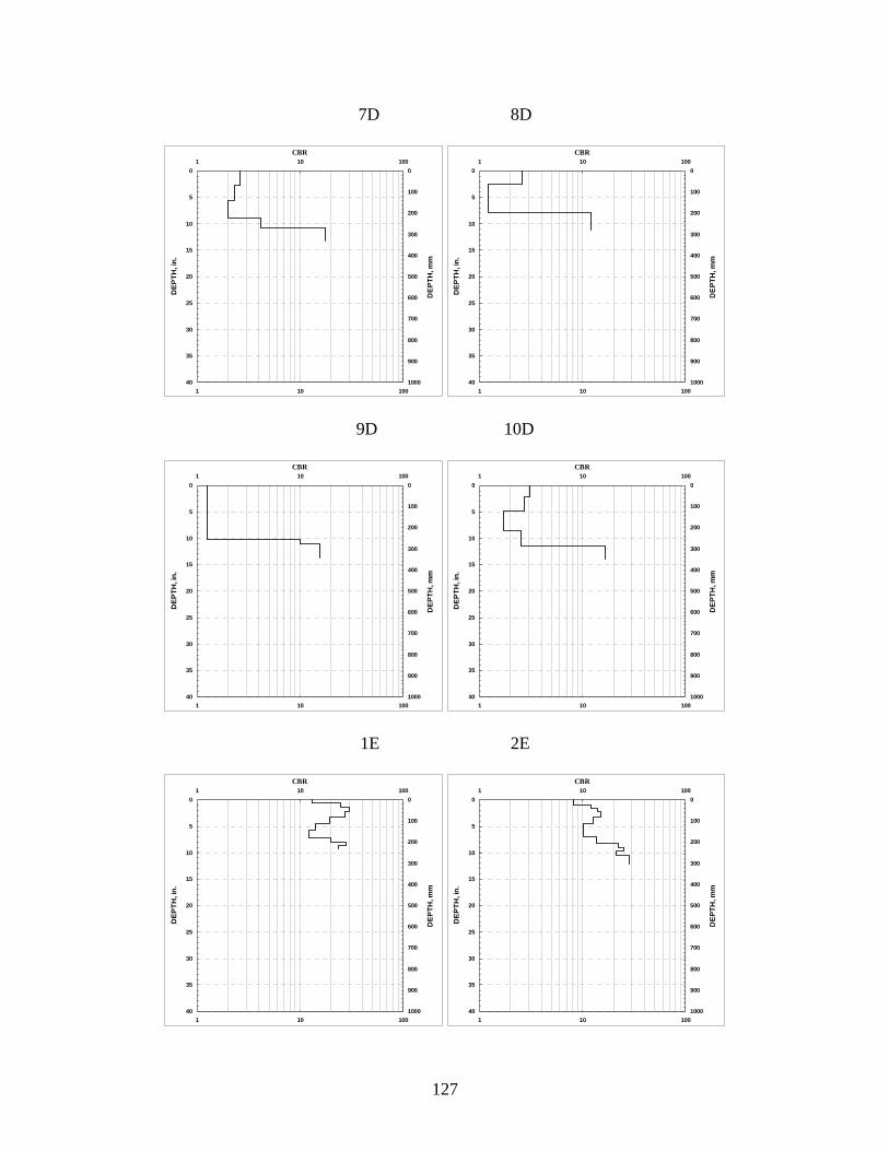
127

7D 8D

0

5

10

15

20

25

30

35

40

1 10 100CBR

DEP

TH, i

n.0

100

200

300

400

500

600

700

800

900

10001 10 100

DE

PTH

, mm

0

5

10

15

20

25

30

35

40

1 10 100CBR

DEP

TH, i

n.

0

100

200

300

400

500

600

700

800

900

10001 10 100

DE

PTH

, mm

9D 10D

0

5

10

15

20

25

30

35

40

1 10 100CBR

DEP

TH, i

n.

0

100

200

300

400

500

600

700

800

900

10001 10 100

DE

PTH

, mm

0

5

10

15

20

25

30

35

40

1 10 100CBR

DEP

TH, i

n.

0

100

200

300

400

500

600

700

800

900

10001 10 100

DE

PTH

, mm

1E 2E

0

5

10

15

20

25

30

35

40

1 10 100CBR

DEP

TH, i

n.

0

100

200

300

400

500

600

700

800

900

10001 10 100

DE

PTH

, mm

0

5

10

15

20

25

30

35

40

1 10 100CBR

DEP

TH, i

n.

0

100

200

300

400

500

600

700

800

900

10001 10 100

DE

PTH

, mm

128

3E 4E

0

5

10

15

20

25

30

35

40

1 10 100CBR

DEP

TH, i

n.0

100

200

300

400

500

600

700

800

900

10001 10 100

DE

PTH

, mm

0

5

10

15

20

25

30

35

40

1 10 100CBR

DEP

TH, i

n.

0

100

200

300

400

500

600

700

800

900

10001 10 100

DE

PTH

, mm

5E 6E

0

5

10

15

20

25

30

35

40

1 10 100CBR

DEP

TH, i

n.

0

100

200

300

400

500

600

700

800

900

10001 10 100

DE

PTH

, mm

0

5

10

15

20

25

30

35

40

1 10 100CBR

DEP

TH, i

n.

0

100

200

300

400

500

600

700

800

900

10001 10 100

DE

PTH

, mm

7E 8E

0

5

10

15

20

25

30

35

40

1 10 100CBR

DEP

TH, i

n.

0

100

200

300

400

500

600

700

800

900

10001 10 100

DE

PTH

, mm

0

5

10

15

20

25

30

35

40

1 10 100CBR

DEP

TH, i

n.

0

100

200

300

400

500

600

700

800

900

10001 10 100

DE

PTH

, mm

129

9E 10E

0

5

10

15

20

25

30

35

40

1 10 100CBR

DEP

TH, i

n.0

100

200

300

400

500

600

700

800

900

10001 10 100

DE

PTH

, mm

0

5

10

15

20

25

30

35

40

1 10 100CBR

DEP

TH, i

n.

0

100

200

300

400

500

600

700

800

900

10001 10 100

DE

PTH

, mm

1F 2F

0

5

10

15

20

25

30

35

40

1 10 100CBR

DEP

TH, i

n.

0

100

200

300

400

500

600

700

800

900

10001 10 100

DE

PTH

, mm

0

5

10

15

20

25

30

35

40

1 10CBR

DEP

TH, i

n.

0

100

200

300

400

500

600

700

800

900

10001 10 100

DE

PTH

, mm

3F 5F

0

5

10

15

20

25

30

35

40

1 10 100CBR

DEP

TH, i

n.

0

100

200

300

400

500

600

700

800

900

10001 10 100

DE

PTH

, mm

0

5

10

15

20

25

30

35

40

1 10CBR

DEP

TH, i

n.

0

100

200

300

400

500

600

700

800

900

10001 10 100

DE

PTH

, mm

130

6F 7F

0

5

10

15

20

25

30

35

40

1 10 100CBR

DEP

TH, i

n.0

100

200

300

400

500

600

700

800

900

10001 10 100

DE

PTH

, mm

0

5

10

15

20

25

30

35

40

1 10CBR

DEP

TH, i

n.

0

100

200

300

400

500

600

700

800

900

10001 10 100

DE

PTH

, mm

8F 9F

0

5

10

15

20

25

30

35

40

1 10CBR

DEP

TH, i

n.

0

100

200

300

400

500

600

700

800

900

10001 10 100

DE

PTH

, mm

0

5

10

15

20

25

30

35

40

1 10 100CBR

DEP

TH, i

n.

0

100

200

300

400

500

600

700

800

900

10001 10 100

DE

PTH

, mm

10F 1G

0

5

10

15

20

25

30

35

40

1 10 100CBR

DEP

TH, i

n.

0

100

200

300

400

500

600

700

800

900

10001 10 100

DE

PTH

, mm

0

5

10

15

20

25

30

35

40

1 10 100CBR

DEP

TH, i

n.

0

100

200

300

400

500

600

700

800

900

10001 10 100

DE

PTH

, mm

131

2G 3G

0

5

10

15

20

25

30

35

40

1 10 100CBR

DEP

TH, i

n.0

100

200

300

400

500

600

700

800

900

10001 10 100

DE

PTH

, mm

0

5

10

15

20

25

30

35

40

1 10 100CBR

DEP

TH, i

n.

0

100

200

300

400

500

600

700

800

900

10001 10 100

DE

PTH

, mm

4G 5G

0

5

10

15

20

25

30

35

40

1 10 100CBR

DEP

TH, i

n.

0

100

200

300

400

500

600

700

800

900

10001 10 100

DE

PTH

, mm

0

5

10

15

20

25

30

35

40

1 10CBR

DEP

TH, i

n.

0

100

200

300

400

500

600

700

800

900

10001 10 100

DE

PTH

, mm

1H 2H

0

5

10

15

20

25

30

35

40

1 10 100CBR

DEP

TH, i

n.

0

100

200

300

400

500

600

700

800

900

10001 10 100

DE

PTH

, mm

0

5

10

15

20

25

30

35

40

1 10 100CBR

DEP

TH, i

n.

0

100

200

300

400

500

600

700

800

900

10001 10 100

DE

PTH

, mm

132

3H 4H

0

5

10

15

20

25

30

35

40

1 10 100CBR

DEP

TH, i

n.

0

100

200

300

400

500

600

700

800

900

10001 10 100

DE

PTH

, mm

0

5

10

15

20

25

30

35

40

1 10 100CBR

DEP

TH, i

n.

0

100

200

300

400

500

600

700

800

900

10001 10 100

DE

PTH

, mm

5H 6H

0

5

10

15

20

25

30

35

40

1 10 100CBR

DEP

TH, i

n.

0

100

200

300

400

500

600

700

800

900

10001 10 100

DE

PTH

, mm

0

5

10

15

20

25

30

35

40

1 10 100CBR

DEP

TH, i

n.

0

100

200

300

400

500

600

700

800

900

10001 10 100

DE

PTH

, mm

7H 8H

0

5

10

15

20

25

30

35

40

1 10 100CBR

DEP

TH, i

n.

0

100

200

300

400

500

600

700

800

900

10001 10 100

DE

PTH

, mm

0

5

10

15

20

25

30

35

40

1 10 100CBR

DEP

TH, i

n.

0

100

200

300

400

500

600

700

800

900

10001 10 100

DE

PTH

, mm

133

9H 10H

0

5

10

15

20

25

30

35

40

1 10 100CBR

DEP

TH, i

n.0

100

200

300

400

500

600

700

800

900

10001 10 100

DE

PTH

, mm

0

5

10

15

20

25

30

35

40

1 10 100CBR

DEP

TH, i

n.

0

100

200

300

400

500

600

700

800

900

10001 10 100

DE

PTH

, mm

134

(a)

(b)

(c)

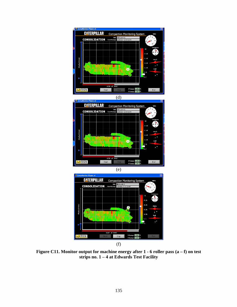
135

(d)

(e)

(f)

Figure C11. Monitor output for machine energy after 1 - 6 roller pass (a – f) on test strips no. 1 – 4 at Edwards Test Facility

136

(a)

(b)

(c)

137

(d)

(e)

(f)

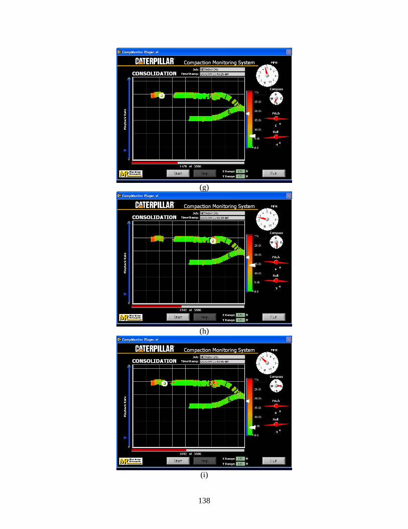
138

(g)

(h)

(i)

139

(j)

Figure C12. Monitor output for machine energy after 1-10 roller passes (a – j) on test strip no. 6 at Edwards Test Facility

(a)

140

(b)

(c)

(d)

141

(e)

(f)

(g)

142

(h)

(i)

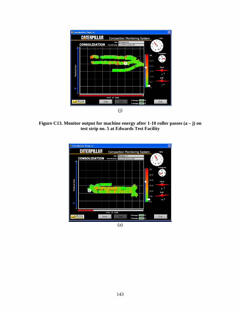
143

(j)

Figure C13. Monitor output for machine energy after 1-10 roller passes (a – j) on test strip no. 5 at Edwards Test Facility

(a)

144

(b)

(c)

(d)

145

(e)

(f)

146

(g)

Figure C14. Monitor output for machine energy after 2-3, 5-9 roller pass (a – g) on

test strip no.7 at Edwards Test Facility

(a)

147

(b)

(c)

(d)

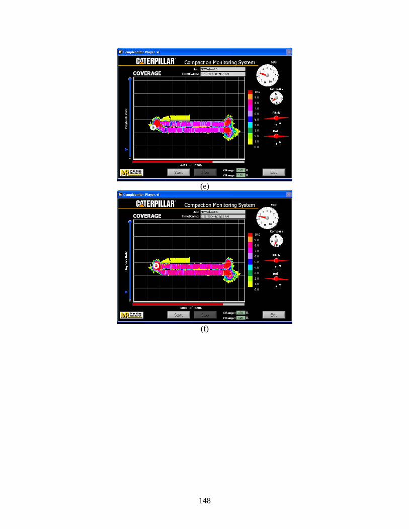
148

(e)

(f)

149

(g)

Figure C15. Monitor output for machine coverage after 2-3, 5-9 roller pass (a –g) on

test strip no.7 at Edwards Test Facility

150

0

20

40

60

80

0 5 10 15 20

Location (m)

Mac

hine

Ene

rgy

(kJ)

Pass 1Pass 3Pass 6

Figure C16. Machine power values as a function of roller pass for test strip 1 at


0

20

40

60

80

0 5 10 15 20

Location (m)

Mac

hine

(kJ)

Pass 1Pass 3Pass 6



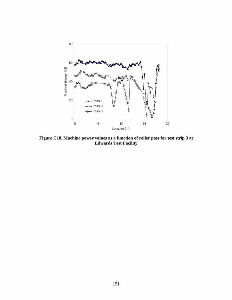
151

0

20

40

60

80

0 5 10 15 20Location (m)

Mac

hine

Ene

rgy

(kJ)

Pass 1Pass 3Pass 6



152

APPENDIX D: STATISTICAL ANALYSIS RESULTS – PROJECT NO. 2

153

Outline of Analysis

I. Soil Property – Engine Power Relationship A. Paired Scatter Plots B. Regression Results a) Soil Properties vs. Gross Power b) Soil Properties vs. Net Power II. Measured Power Values A. Box Plots a) Gross Power b) Net Power B. Summary Statistics a) Gross Power b) Net Power III. Measured Soil Properties A. Box Plots B. Summary Statistics

154

I. Soil Properties – Engine Power Relationship - A. Paired Scatter Plots:

8 10 12 14 16 18 4 6 8 10 14 20 30 40 1.3 1.4 1.5 1.6 1_7

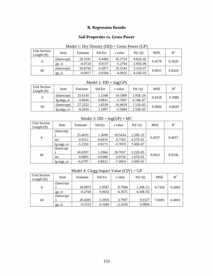
155

B. Regression Results

Soil Properties vs. Gross Power

Model 1: Dry Density (DD) = Gross Power (GP) Unit Section Length (ft) Item Estimate Std.Err t value Pr(>|t|) MSE R2

(Intercept) 20.3241 0.4460 45.5724 8.81E-42 6 gp_si -0.0724 0.0137 -5.2794 2.95E-06

0.4578 0.3626


0.0831 0.8324

Model 2: DD = log(GP)

Unit Section Length (ft) Item Estimate Std.Err t value Pr(>|t|) MSE R2

(Intercept) 25.6145 1.3348 19.1899 1.95E-24 6 lg.mgp_si -5.0916 0.8931 -5.7007 6.74E-07

0.4318 0.3988


0.0684 0.8620

Model 3: DD = log(GP) + MC


(Intercept) 25.4035 1.3699 18.5434 1.59E-23 mc 0.0312 0.0416 0.7505 4.57E-01 6

lg.mgp_si -5.2350 0.9173 -5.7070 7.00E-07

0.4357 0.4057

(Intercept) 26.8397 1.2964 20.7037 3.22E-05 mc 0.0805 0.0388 2.0756 1.07E-01 60

lg.mgp_si -6.6797 0.8912 -7.4954 1.69E-03

0.0412 0.9336

Model 4: Clegg Impact Value (CIV) = GP



9.7358 0.2802

(Intercept) 20.4381 5.3916 3.7907 0.0127 60 gp_si -0.3553 0.1690 -2.1029 0.0894

7.0085 0.4693

156

Model 5: CIV = log(GP)



9.6243 0.2884

(Intercept) 43.9766 16.9264 2.5981 0.0484 60 lg.mgp_si -23.3116 11.3577 -2.0525 0.0953

7.1678 0.4573

Model 6: CIV = log(GP) + MC


(Intercept) 44.3375 4.2457 10.4430 6.01E-14mc -1.0371 0.1289 -8.0434 1.89E-106

lg.mgp_si -14.0270 2.8428 -4.9342 1.01E-05

4.1846 0.6969

(Intercept) 49.3154 4.2974 11.4757 3.29E-04mc -1.1145 0.1285 -8.6715 9.73E-0460

lg.mgp_si -16.6893 2.9542 -5.6493 4.84E-03

0.4525 0.9726

Model 7: Mean Dynamic Cone Penetrometer value (MDCP) = GP


(Intercept) -3.1948 14.4792 -0.2206 0.8263 6 gp_si 1.6679 0.4449 3.7486 0.0005

482.5413 0.2229

(Intercept) -20.7817 41.4723 -0.5011 0.6376 60 gp_si 2.2936 1.2998 1.7646 0.1379

414.6695 0.3838

Model 8: MDCP = log(GP)


(Intercept) -119.8148 44.4048 -2.6982 0.0095 6 lg.mgp_si 113.7932 29.7124 3.8298 0.0004

477.8768 0.2304

(Intercept) -173.2376 129.5868 -1.3368 0.2389 60 lg.mgp_si 150.8197 86.9529 1.7345 0.1434

420.1212 0.3757

Model 9: MDCP = log(GP) + MC


(Intercept) -171.0465 28.3416 -6.0352 2.22E-07 mc 7.5806 0.8607 8.8076 0.0000 6 lg.mgp_si 78.9568 18.9772 4.1606 1.31E-04

186.4728 0.7058

(Intercept) -211.9168 56.6437 -3.7412 2.01E-02 mc 8.0742 1.6940 4.7663 0.0089 60 lg.mgp_si 102.8416 38.9395 2.6411 0.0575

78.6228 0.9065

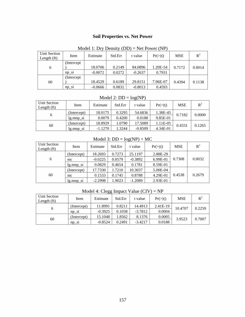
157

Soil Properties vs. Net Power

Model 1: Dry Density (DD) = Net Power (NP) Unit Section Length (ft) Item Estimate Std.Err t value Pr(>|t|) MSE R2

(Intercept) 18.0706 0.2149 84.0896 1.20E-54 6 np_si -0.0072 0.0272 -0.2637 0.7931

0.7172 0.0014

(Intercept) 18.4529 0.6189 29.8151 7.96E-07 60 np_si -0.0666 0.0831 -0.8013 0.4593

0.4394 0.1138

Model 2: DD = log(NP)


(Intercept) 18.0175 0.3295 54.6836 1.38E-45 6 lg.mnp_si 0.0079 0.4200 0.0188 9.85E-01

0.7182 0.0000


0.4331 0.1265

Model 3: DD = log(NP) + MC


(Intercept) 18.2693 0.7273 25.1197 2.88E-29 mc -0.0225 0.0579 -0.3892 6.99E-01 6 lg.mnp_si 0.0829 0.4654 0.1781 8.59E-01

0.7308 0.0032


0.4538 0.2679

Model 4: Clegg Impact Value (CIV) = NP


(Intercept) 11.8991 0.8211 14.4913 2.41E-19 6 np_si -0.3925 0.1038 -3.7812 0.0004

10.4707 0.2259

(Intercept) 15.1048 1.8562 8.1376 0.0005 60 np_si -0.8524 0.2491 -3.4217 0.0188

3.9523 0.7007

158

Model 5: CIV = log(NP) Unit Section Length (ft) Item Estimate Std.Err t value Pr(>|t|) MSE R2


10.6157 0.2152


4.0550 0.6930

Model 6: CIV = log(NP) + MC


(Intercept) 25.3042 2.0643 12.2581 2.15E-16 mc -1.0438 0.1643 -6.3522 7.25E-08 6

lg.mnp_si -2.4431 1.3210 -1.8494 7.06E-02

5.8876

0.5736

(Intercept) 26.4408 3.9924 6.6227 2.70E-03 mc -0.8395 0.4047 -2.0743 1.07E-01 60

lg.mnp_si -7.1912 4.4130 -1.6296 1.79E-01

2.4420

0.8521

Model 7: Mean Dynamic Cone Penetrometer value (MDCP) = NP


(Intercept) 29.8067 5.3107 5.6126 9.20E-07 6 np_si 3.0375 0.6714 4.5240 3.87E-05

437.9821 0.2946

(Intercept) 10.9742 14.1750 0.7742 0.4738 60 np_si 5.8935 1.9024 3.0979 0.0269

230.4914 0.6575

Model 8: MDCP = log(NP)


(Intercept) 19.0381 8.4621 2.2498 0.0290 6 lg.mnp_si 42.0879 10.7856 3.9022 0.0003

473.7118 0.2371

(Intercept) -21.0727 26.6055 -0.7920 0.4642 60 lg.mnp_si 91.0705 32.6548 2.7889 0.0385

263.3092 0.6087

Model 9: MDCP = log(NP) + MC


(Intercept) -64.0212 12.9742 -4.9345 1.01E-05 mc 7.4336 1.0328 7.1974 0.0000 6

lg.mnp_si 17.3446 8.3025 2.0891 4.20E-02

232.5765 0.6331

(Intercept) -71.2995 32.8029 -2.1736 9.54E-02 mc 6.6389 3.3252 1.9966 0.1166 60

lg.mnp_si 40.2843 36.2580 1.1110 0.3288

164.8514 0.8040

159


A. Box Plots Gross Power

Gross Power Section A

g r--------------------------------------.

Number of Passes

Gross Power Section C g r------------------------------------.

0

"

o~ ' !

Number of Passes

Gross Power Section F

Number of Passes

Gross Power Section H

10

g r--------------------------------------.

10

Number of Passes

0 0

0

"

0

"'

Gross Power Section B

Number of Passes

Gross Pow er Section 0

-+-

Number of Passes

Gross Power Section G

Number of Passes

10

160

Net Power

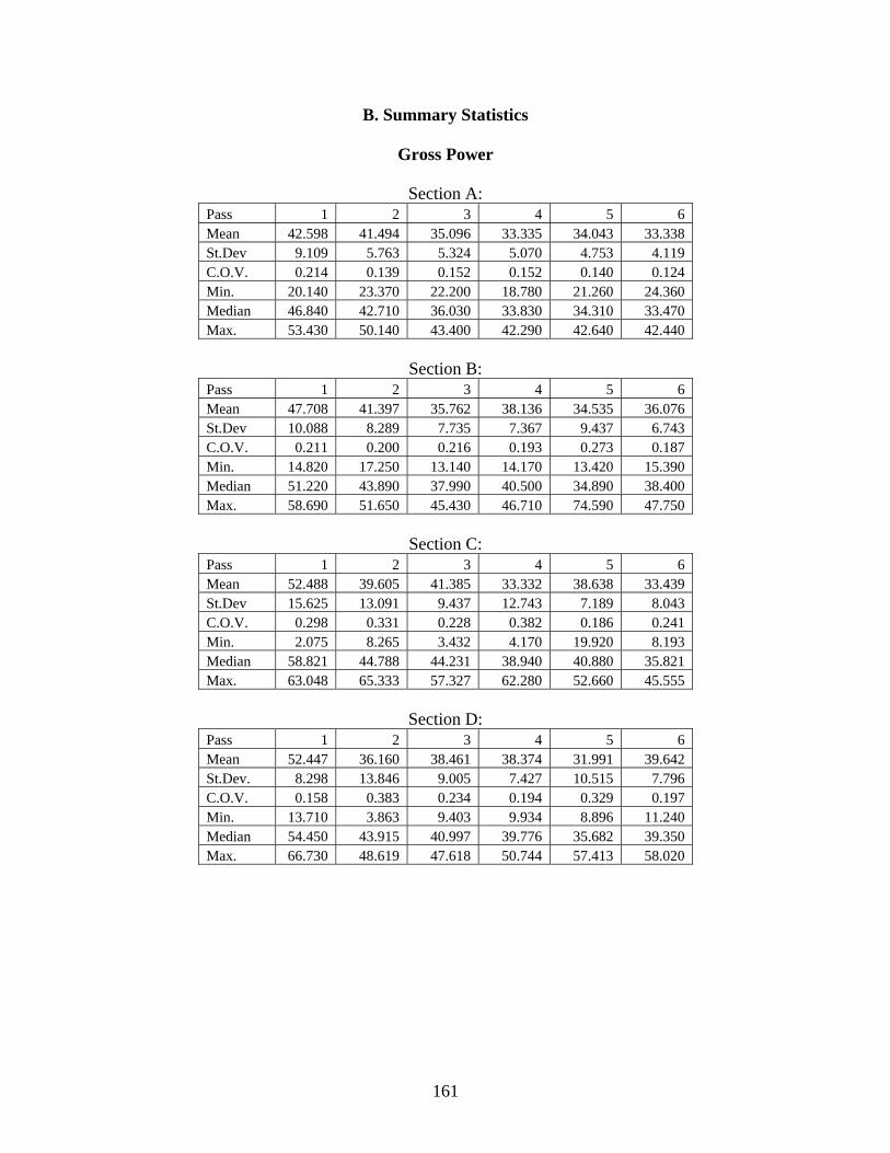
161


Gross Power

Section A: Pass 1 2 3 4 5 6 Mean 42.598 41.494 35.096 33.335 34.043 33.338 St.Dev 9.109 5.763 5.324 5.070 4.753 4.119 C.O.V. 0.214 0.139 0.152 0.152 0.140 0.124 Min. 20.140 23.370 22.200 18.780 21.260 24.360 Median 46.840 42.710 36.030 33.830 34.310 33.470 Max. 53.430 50.140 43.400 42.290 42.640 42.440

Section B:

Pass 1 2 3 4 5 6 Mean 47.708 41.397 35.762 38.136 34.535 36.076 St.Dev 10.088 8.289 7.735 7.367 9.437 6.743 C.O.V. 0.211 0.200 0.216 0.193 0.273 0.187 Min. 14.820 17.250 13.140 14.170 13.420 15.390 Median 51.220 43.890 37.990 40.500 34.890 38.400 Max. 58.690 51.650 45.430 46.710 74.590 47.750

Section C:


Section D:

Pass 1 2 3 4 5 6 Mean 52.447 36.160 38.461 38.374 31.991 39.642 St.Dev. 8.298 13.846 9.005 7.427 10.515 7.796 C.O.V. 0.158 0.383 0.234 0.194 0.329 0.197 Min. 13.710 3.863 9.403 9.934 8.896 11.240 Median 54.450 43.915 40.997 39.776 35.682 39.350 Max. 66.730 48.619 47.618 50.744 57.413 58.020

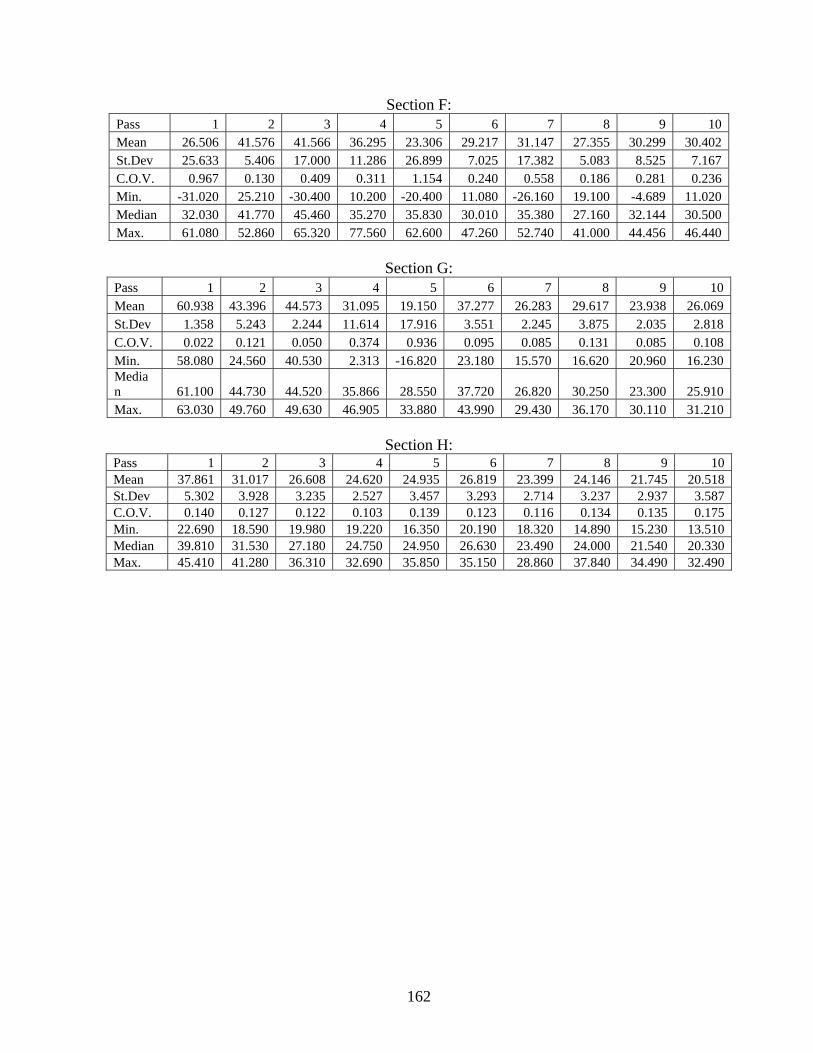
162

Section F: Pass 1 2 3 4 5 6 7 8 9 10 Mean 26.506 41.576 41.566 36.295 23.306 29.217 31.147 27.355 30.299 30.402 St.Dev 25.633 5.406 17.000 11.286 26.899 7.025 17.382 5.083 8.525 7.167 C.O.V. 0.967 0.130 0.409 0.311 1.154 0.240 0.558 0.186 0.281 0.236 Min. -31.020 25.210 -30.400 10.200 -20.400 11.080 -26.160 19.100 -4.689 11.020 Median 32.030 41.770 45.460 35.270 35.830 30.010 35.380 27.160 32.144 30.500 Max. 61.080 52.860 65.320 77.560 62.600 47.260 52.740 41.000 44.456 46.440

Section G:

Pass 1 2 3 4 5 6 7 8 9 10 Mean 60.938 43.396 44.573 31.095 19.150 37.277 26.283 29.617 23.938 26.069 St.Dev 1.358 5.243 2.244 11.614 17.916 3.551 2.245 3.875 2.035 2.818 C.O.V. 0.022 0.121 0.050 0.374 0.936 0.095 0.085 0.131 0.085 0.108 Min. 58.080 24.560 40.530 2.313 -16.820 23.180 15.570 16.620 20.960 16.230 Median 61.100 44.730 44.520 35.866 28.550 37.720 26.820 30.250 23.300 25.910 Max. 63.030 49.760 49.630 46.905 33.880 43.990 29.430 36.170 30.110 31.210

Section H:

Pass 1 2 3 4 5 6 7 8 9 10 Mean 37.861 31.017 26.608 24.620 24.935 26.819 23.399 24.146 21.745 20.518 St.Dev 5.302 3.928 3.235 2.527 3.457 3.293 2.714 3.237 2.937 3.587 C.O.V. 0.140 0.127 0.122 0.103 0.139 0.123 0.116 0.134 0.135 0.175 Min. 22.690 18.590 19.980 19.220 16.350 20.190 18.320 14.890 15.230 13.510 Median 39.810 31.530 27.180 24.750 24.950 26.630 23.490 24.000 21.540 20.330 Max. 45.410 41.280 36.310 32.690 35.850 35.150 28.860 37.840 34.490 32.490

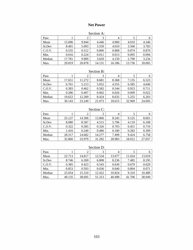
163

Net Power

Section A: Pass 1 2 3 4 5 6 Mean 15.696 9.944 4.446 4.960 4.010 4.346 St.Dev 8.401 5.093 3.559 4.010 3.506 3.783 C.O.V. 0.535 0.512 0.800 0.808 0.874 0.870 Min. 0.016 0.224 0.011 0.013 0.095 0.094 Median 17.781 9.969 3.659 4.150 2.790 3.234 Max. 29.819 20.878 14.131 16.186 13.736 18.005

Section B:


Section C:


Section D:


164

Section F: Pass 1 2 3 4 5 6 7 8 9 10 Mean 16.006 13.749 15.285 13.602 12.510 5.704 8.160 7.657 5.974 6.595 St.Dev 10.796 5.105 6.049 12.338 9.172 5.166 6.273 7.045 4.326 6.400 C.O.V. 0.675 0.371 0.396 0.907 0.733 0.906 0.769 0.920 0.724 0.970 Min. 0.169 4.009 2.821 0.033 0.850 0.093 0.217 0.013 0.011 0.140 Median 15.342 13.479 15.757 8.953 12.111 4.492 6.053 4.896 6.040 5.013 Max. 45.312 32.138 38.967 55.251 37.956 29.902 25.009 22.157 22.149 33.004

Section G:


Section H:


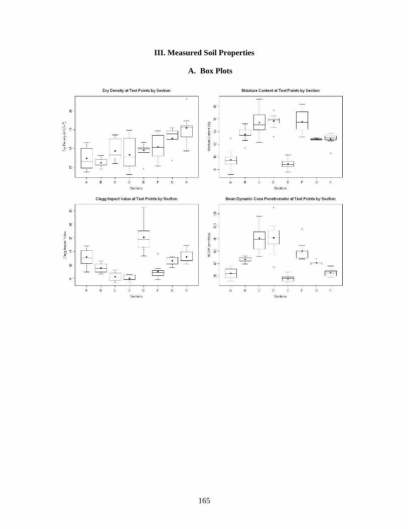
165

III. Measured Soil Properties

A. Box Plots

Dry Density at Test Points by Section Moisture Content at Test Points by Section

'!! R

B 'f' ~bj~ ~ ~ T ~ sD

~ : ~ z ~ 1: ;! c::;::J : . 6 g

g~nQMtr ~ 0 = E;i3 .

~ 0

0 '!! ~

"' 8 ~ ' ' ' ' ¢ ~ ' ~ ~ :

~

~ ~

A 0 G H A 0 G H

Sections Sections

Clegg Impact Value at Test Points by Section Mean Dynamic Cone Penetrometer at Test Points by Section

li! B

i'1 §

:; R B ~ 0:1 EJB ~

_§ .s o_

iii EJ 'f'

B ~ E O 0 . 0

<:3 "' I • I

"' l9 " =

8c+J c=J B ' R

$ A 0 G H A 0 G H

Sections Sections

166


Section A

MC(%) DD(KN/m3) CIV MDCP

(mm/blow) Mean 9.525 17.479 13.000 23.900 St.Dev 1.556 0.551 3.102 8.359 C.O.V. 0.163 0.032 0.239 0.350 Max. 12.900 18.320 17.200 37.000 Median 9.450 17.320 12.750 24.000 Min. 7.200 16.750 7.500 12.000

Section B



Section C



Section D



167

Section E



Section F



Section G



Section H



168

APPENDIX E: LABORATORY AND FIELD TEST RESULTS – PROJECT NO. 3

169

(a)

(b)

(c)

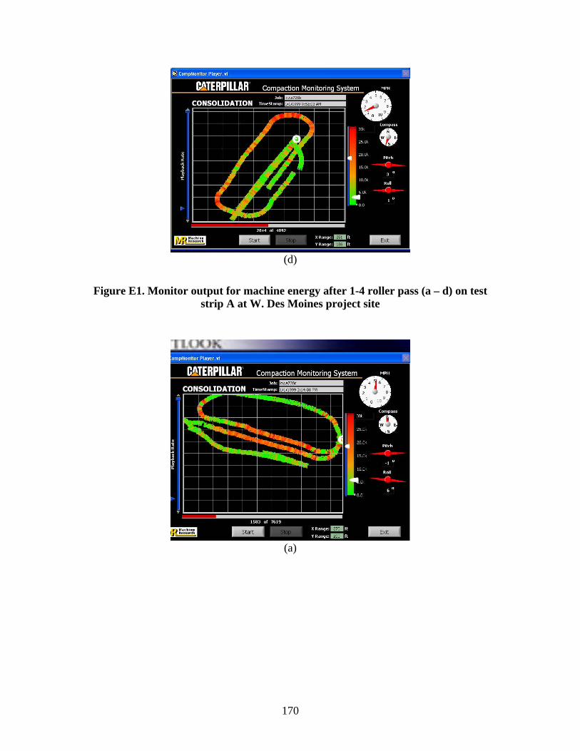
170

(d)

Figure E1. Monitor output for machine energy after 1-4 roller pass (a – d) on test

strip A at W. Des Moines project site

(a)

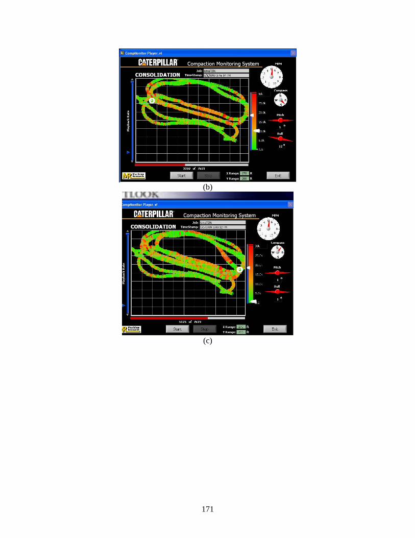
171

(b)

(c)

172

(d)

Figure E2. Monitor output for machine energy after 1, 2, 4, and 6 roller pass (a – d)

on test strips C and CV at W. Des Moines project site

173

APPENDIX F: STATISTICAL ANALYSIS RESULTS – PROJECT NO. 3

174

Outline of Analysis

I. Soil Property – Engine Power Relationship A. Paired Scatter Plots B. Regression Results a) Soil Properties vs. Gross Power b) Soil Properties vs. Net Power II. Measured Power Values A. Box Plots a) Gross Power b) Net Power B. Summary Statistics a) Gross Power b) Net Power III. Measured Soil Properties A. Box Plots B. Summary Statistics

175

I. Soil Property and Power Value Relationship

A. Paired Scatter Plots

Paired Scatter Plot for Des Moines Test, StripA 11.0 12.5 14.0 100 200

~o o 0 o o 0 • o 0 0~

oOOo o

2 6 10 14

0 0~ % oooo o o

0.4 0.8

G 0 0 ° g 0 0 ° g 0~ 0 :0 0 0

me L_ ___ : __ ~_J L_ _____ o __ o~~J L~------_J ~--------J L----~--_J ~:::::;::~ ~::::::~~ : qB ~ 8 o ) :0 o o ~o ~ oo% o ~ o o

: ~=oo::=!::o::~o dd_si L__0 __

0

_0._:_o_:_OJ

0

~8=0

~0:~::0 0::0

::~ o o .. o ..

00

0 0

0 ..

8

0 0

0

0 0

0 0 0 ooo 0 o 0 o o

0 0

0

8

q ... G 0 0 1<>0 0 oO 0 0 ooO 00

oO Q o o o o o o<b oo g o Cb o o o oo o Cb Cb g oo o Oo ~

cv L2_0_; ______ _J ~~0:::::0:::0~ ~==~:::0:::0~0 ~==~====~ ~====~==:; :

B 00 0 ~ 0

0 0 0 0

0

o o ;~o o

~

0

oo o o~o o 0 0

~ 0 0

0

oooo:.o8

0

0

0 ~ :~ 0 0 0 0

~ -.==8 °==0::::;;=:=:~0

~0=0=0=:·=0

=8~:~~:~0 ~=0;0

=~= .. =:=0 =~=~~0 ~··=00~0

:~:0=00====~· B ,._,p_ .. _ .... o~:-0

-0

-.. -

0

JT2J "-'--0-0-~~0'-':'-0

-~Jo : :::: o::o::::;;::;;;~ ~o '-::~::o:ooo:o::;:~o:=;~o '-:::o;::::'l.~:~:=;=~~o ~:o:oo:,o;;8o:o o:::;o;:::~o "':::"'.:oo:::o:~o:o:o~; B "-'--"'-o_oo_ .. _;_o_oJo[ r-o---o --......,,.,_1

r 0 0 r 0 0 r 0 0 ~t~ 00 r ~ 0 000

0000o EJ 0 o ~

o o ~So o 'aOoo o ~ ~ o o •:o 9odJo o : :o

:00 000 0 0 ~00 OoOOO 0 $,PO ,P~ lg.mgp_si oO~ ~

0 0 0 0 0

:=0 ::::;:::;::~ ~==::::"'~ ~~0 ~-- ~oO ;::::::~ ~::::::;::::~ ..._0 ---2..:0 0'-------J r--~ 0 0 ....,

• ;~ • -.:-·~ • • : •?' ::~:. • • : ,,..:·:· •: [ .. /'1.,..,..,8-0T:...,:r~T0

-0

,-J: llg mop_,; I 22 26 30 1.0 2.5 4.0 20 40 1.1 1.3 1.5 1.7

176

Paired Scatter Plot for Des Moines Test, StripB 12.5 13.5 14.5 100 200 10 20 30 1.0 1.3 1.6

G 0 0 0 0 0 0

0 0 0 0 0 0 0

oo 00 ":o

#00 0 0 0 oo 0 oo<> 0 0 0 oOO 0 08 0

0 0 0 0 0

0 0 0 oo 0 o: 0 0 oo 0

0 : 0 0

0 ooo::oo \0 oo • 0 00 ~0 0 oO o o 0

o oO

0 \o 0

0 Oo 0

"b. 0 8 0 0

~0 Oo 0 0 0 0 0 0 8 0 0 0 0

0 0 0 0 0 0

"1 • %0 ;! g 0 0

"1 0 0 0 0

\2 0 0

~ 0

"1

"' B 0

0 0 00:, ~ 0 ooo

0 ooo o8

0 Oo 0 oo 0 oo 0

0 8 0 ., 0 0

0.

0 oo 0 o'l>

0 q,o

Oo 0 oq, 0 0 0 'l>o 0 0 0 0 'l>o 0 0

:o 00 0 0

0 0 00 0 0 0 00

oq, g 'l. 0 0 .. o ., 0 0 0 0 .. o Oo

0 0 0 0 0

"' Oo 0 0 0 0 0 0 0 0

0 0 0~

O:o4 o

0

G 0 0 0

00 0 0 0 0 0 0 0 0 ., Oo

0 0 0 • 0 00 0 • 0 0

0 0

:! 0 ~0 Oo 0 0 0 0: 0 Ooo 0 0: 0 0 0 o:o 0000 0 0 0 0 r.Po ~o ooO:ooo:o 0

0 0 0 00

00 0 0 0 0~0 o8 0 0 0 0 0 goo~

0 0 0 0 0 0

...

0 0

"' 0 0

0 oq. <?.Oo

0 ~ o~ %o Q

0 0 0 0 B 0 0 0 0 0 0

0 0

0 0 0

0 0

0 0

0 0

Oo 0 ~0 0 0 s'l>o 0 0 ., o8 0 Oo o600J0

0 Oro o$ o Oo 0 6'0~ 0

0 0 0

0 oo

• o'l>o ~ ~0 0 0 o '?. of'o o o •• 00 0 0

'?. 0~ 00 0 .,. .. 0

'l.

<l'o g 0 0

o® og o 0

0 0

0 00 0 °o 0

0 0 0 0 B 00

0 0 [2] .. 0

0

8 Oo 0 0 ~0 0

-.,o 0 .. 0 0 0

~0 0 0 oO 0 0 0 0 0 0 0 0 0

0 0 "'o oo 0~ 0

.. .. t 0 0 ~0 q. 0

8>0 •

~go 0 0 0 0

0 .. 0 ~g / ~

0 0 0 0 0

0

"' 0

00

"' ts ~:! ~ 0 'l> 0

0 ·a 0 0 [] 0 00 0 00

• 0 0 0

o o.,o~ 0 04 0 00 ./ o<b o o o<b o o

0 Oo f{' 'l.

0 0 0 0 oo 0 :0~ • co~o o eo 00

0 0 0

oOJ> 0 0 0 0 0 <PO

0 0 % 0

00 0 °o 0 00 0

<l'o 8 8 Oo 0 0 ~0 0

"'0 0

0 0 oO 0 0 0 0 0

0® o: 0 0 0 "'o oo 0~ 0

.. .. t 00

0 o~o 0 0 0 'l>

0 0 0 ·o 0 0

llgmgp_,; I .. 0 0

oO~ ... 0 0 .. 0 0

0

0 0 0 0 " / 0 &0 q. 0 ~0 (>

~0 Oo "' "1

<Q

00 0 0

Oo f{' %

<'1 0 0., 0 0 0 0 oo 0~

8g ~ooo % Cb~0

o jO Oo : ~ 0 0 0

q 'l.o o%0 .,o 0

0 0 0

0 .[2] 0 0

llgmop_,; I 00 'l. o•o 00

• 0 0 / 0 0 0

0~ "l> 0~ "'

0 0 0 0 0 00 0 00

20 24 2 3 4 5 35 45 55 65 1.55 1.70

177

B. Regression Parameters

Soil Properties vs. GP

DD = GP Strip Item Estimate Std.Err t value Pr(>|t|) MSE R2

(Intercept) 12.8913 0.5480 23.5257 5.74E-15 A gp_si 0.0029 0.0163 0.1765 8.62E-01

0.9020 0.0017

(Intercept) 15.6109 0.6653 23.4636 1.45E-17 B gp_si -0.0392 0.0139 -2.8248 9.61E-03

0.3570 0.2576

DD = log(GP)

Strip Item Estimate Std.Err t value Pr(>|t|) MSE R2 (Intercept) 13.0413 1.5156 8.6047 8.55E-08 A lg.mgp_si -0.0420 1.0362 -0.0405 9.68E-01

0.9035 0.0001

(Intercept) 21.0222 2.5093 8.3776 1.93E-08 B lg.mgp_si -4.3580 1.5046 -2.8965 8.14E-03

0.3523 0.2673

DD = MC + log(GP)

Strip Item Estimate Std.Err t value Pr(>|t|) MSE R2 (Intercept) 15.4242 2.1930 7.0334 2.01E-06 Mc -0.1599 0.1092 -1.4640 1.61E-01 A lg.mgp_si 1.3533 1.3849 0.9771 3.42E-01

0.8496 0.1120

(Intercept) 21.6186 2.2985 9.4053 3.64E-09 mc -0.1376 0.0574 -2.3953 2.56E-02 B lg.mgp_si -2.8520 1.5074 -1.8919 7.17E-02

0.2922 0.4188

CIV = GP

Strip Item Estimate Std.Err t value Pr(>|t|) MSE R2 (Intercept) 3.3739 0.5119 6.5906 3.44E-06 A gp_si -0.0067 0.0152 -0.4427 6.63E-01

0.7873 0.0108

(Intercept) 5.0145 1.0165 4.9330 0.0001 B gp_si -0.0342 0.0212 -1.6105 0.1209

0.8334 0.1013

CIV = log(GP) Strip Item Estimate Std.Err t value Pr(>|t|) MSE R2

(Intercept) 4.2134 1.4004 3.0087 0.0075 A lg.mgp_si -0.7239 0.9575 -0.7561 0.4594

0.7714 0.0308

(Intercept) 9.4732 3.8689 2.4486 0.0224 B lg.mgp_si -3.6431 2.3197 -1.5705 0.1300

0.8376 0.0969

CIV = MC + log(GP)

Strip Item Estimate Std.Err t value Pr(>|t|) MSE R2 (Intercept) 6.7268 1.9872 3.3851 0.0035 mc -0.1687 0.0990 -1.7041 0.1066 A lg.mgp_si 0.7478 1.2550 0.5959 0.5591

0.6976 0.1722

178

(Intercept) 10.1154 3.7732 2.6809 0.0137 mc -0.1481 0.0943 -1.5712 0.1304 B lg.mgp_si -2.0215 2.4745 -0.8169 0.4227

0.7873 0.1880

MDCP = GP

Strip Item Estimate Std.Err t value Pr(>|t|) MSE R2 (Intercept) 88.4505 21.3514 4.1426 0.0006 A gp_si 0.3603 0.6332 0.5690 0.5764

1369.5080 0.0177

(Intercept) 104.7484 55.0886 1.9015 0.0698 B gp_si 0.4613 1.1503 0.4010 0.6921

2447.5940 0.0069

MDCP = log(GP) Strip Item Estimate Std.Err t value Pr(>|t|) MSE R2

(Intercept) 47.8130 58.2421 0.8209 0.4224 A lg.mgp_si 35.7955 39.8209 0.8989 0.3806

1334.2460 0.0430

(Intercept) 65.3689 209.4856 0.3120 0.7578 B lg.mgp_si 36.6825 125.6048 0.2920 0.7729

2455.6000 0.0037

MDCP = MC + log(GP)

Strip Item Estimate Std.Err t value Pr(>|t|) MSE R2 (Intercept) -18.1128 86.7941 -0.2087 0.8372 mc 4.4237 4.3227 1.0234 0.3205 A lg.mgp_si -2.8075 54.8129 -0.0512 0.9597

1330.7500 0.0985

(Intercept) 36.6502 207.9154 0.1763 0.8617 mc 6.6246 5.1953 1.2751 0.2156 B lg.mgp_si -35.8363 136.3560 -0.2628 0.7951

2390.5410 0.0723

179

Soil Properties vs. NP

DD = NP Strip Item Estimate Std.Err t value Pr(>|t|) MSE R2

(Intercept) 12.3205 0.4922 25.0339 1.94E-15 A np_si 0.0860 0.0586 1.4689 1.59E-01

0.8069 0.1070

(Intercept) 14.7577 0.2491 59.2356 1.19E-26 B np_si -0.0561 0.0128 -4.3838 2.16E-04

0.2620 0.4552

DD = log(NP)

Strip Item Estimate Std.Err t value Pr(>|t|) MSE R2 (Intercept) 11.9881 0.7399 16.2013 3.53E-12 A lg.mnp_si 1.1956 0.8576 1.3941 1.80E-01

0.8155 0.0974

(Intercept) 16.9095 0.6283 26.9121 6.88E-19 B lg.mnp_si -2.6045 0.5139 -5.0681 3.94E-05

0.2272 0.5276

DD = MC + log(NP)

Strip Item Estimate Std.Err t value Pr(>|t|) MSE R2 (Intercept) 15.5294 2.0137 7.7118 5.99E-07 mc -0.1467 0.0783 -1.8731 7.84E-02 A lg.mnp_si 1.7958 0.8650 2.0761 5.34E-02

0.7158 0.2518

(Intercept) 17.5755 1.0566 16.6338 6.03E-14 mc -0.0491 0.0623 -0.7876 4.39E-01 B lg.mnp_si -2.2388 0.6958 -3.2178 3.96E-03

0.2310 0.5405

CIV = NP

Strip Item Estimate Std.Err t value Pr(>|t|) MSE R2 (Intercept) 3.2490 0.4883 6.6536 3.04E-06 A

np_si -0.0109 0.0581 -0.1883 8.53E-01 0.7943 0.0020

(Intercept) 4.2988 0.4217 10.1937 5.32E-10 B np_si -0.0504 0.0217 -2.3273 2.91E-02

0.7506 0.1906

CIV = log(NP)

Strip Item Estimate Std.Err t value Pr(>|t|) MSE R2 (Intercept) 3.3128 0.7301 4.5376 0.0003 A lg.mnp_si -0.1780 0.8462 -0.2104 0.8357

0.7939 0.0025

(Intercept) 6.1799 1.1264 5.4866 1.41E-05 B lg.mnp_si -2.2970 0.9212 -2.4934 2.03E-02

0.7300 0.2128

180

CIV = MC + log(NP) Strip Item Estimate Std. Err t value Pr(>|t|) MSE R2

(Intercept) 6.7296 1.9958 3.3719 0.0036 mc -0.1415 0.0776 -1.8235 0.0859 A lg.mnp_si 0.4011 0.8573 0.4679 0.6458

0.7031 0.1656

(Intercept) 7.2309 1.9001 3.8055 0.0010 mc -0.0775 0.1121 -0.6911 0.4967 B lg.mnp_si -1.7199 1.2512 -1.3746 0.1831

0.7470 0.2295

MDCP = NP

Strip Item Estimate Std .Err t value Pr(>|t|) MSE R2 (Intercept) 95.7495 20.4326 4.6861 0.0002 A np_si 0.5084 2.4313 0.2091 0.8367

1390.7630 0.0024

(Intercept) 109.1856 23.8393 4.5801 1.33E-04 B np_si 0.9746 1.2248 0.7957 4.34E-01

2398.6710 0.0268

MDCP = log(NP) Strip Item Estimate Std. Err t value Pr(>|t|) MSE R2

(Intercept) 85.9057 30.4078 2.8251 0.0112 A lg.mnp_si 16.5582 35.2427 0.4698 0.6441

1377.2520 0.0121

(Intercept) 72.6475 64.4537 1.1271 0.2713 B lg.mnp_si 44.5445 52.7158 0.8450 0.4068

2390.4960 0.0301

MDCP = MC + log(NP)

Strip Item Estimate Std. Err t value Pr(>|t|) MSE R2 (Intercept) -18.0821 86.8315 -0.2082 0.8375 mc 4.3071 3.3767 1.2755 0.2193 A lg.mnp_si -1.0673 37.2984 -0.0286 0.9775

1330.8910 0.0984

(Intercept) -10.3406 107.6585 -0.0960 0.9244 mc 6.1162 6.3497 0.9632 0.3459 B lg.mnp_si -1.0214 70.8910 -0.0144 0.9886

2398.0240 0.0694

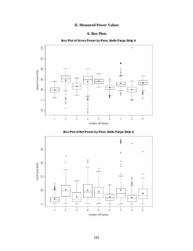
181


A. Box Plots

0 0

0 00

0

0

0

' ----'-

0 0

J_

Box Plot of Gross Power by Pass, Wells Fargo Strip A

~

' ' ' ' '

B~B? ----'-

0

0

0 e 8 0

0

' --'-

0

0

8 0 0

Number of Passes

8

• 0 0

~ --4---

0

Box Plot of Net Power by Pass, Wells Fargo Strip A

0

0

~

'

'

0 0 0

0

~

' ' ' ' ' ' ' ' '

8

0

0 0

0

' ' ' '

0

8 0

-+- l j_

6 T

8

0

0

B ' ' ' ' '

gBag .BB n:. D .. ' ' ' ----'-

2

--'- ----'- ----'-

3 4 5

' ----'-

6

Number of Passes

7

' ----'-

8

' ----'-

9

182

Box Plot of Gross P

0

0

0

Wells Fargo Strip B ower by Pass,

0

0

0

----'t- 8 '

0

BBg~ ' ' ' ' ' ' '

' ---'----

' ' ---'---

g 0

' ' ---'---

' ' ---'---

0 0

8

' ---'------a- 0

4

Number of Passes

Box Plot o fNetPower . B lis Fargo Stnp byPass, We

2 3

' ---'---

4

' ---'---

5

Number of Passes

'

B~ ---'----

6 7 8

183


Gross Power

Strip A: Pass 1 Pass 2 Pass 3 Pass 4 Pass 5 Pass 6 Pass 7 Pass 8 Pass 9

Mean 19.588 38.480 26.419 35.414 36.535 23.944 32.695 20.328 33.201 Std. Dev. 5.893 13.588 8.051 17.805 5.982 6.604 10.995 9.255 7.773

C.O.V. 0.301 0.353 0.305 0.503 0.164 0.276 0.336 0.455 0.234 Min 4.577 -15.719 9.226 -24.265 25.122 4.785 10.720 -0.064 3.037

Median 19.799 41.140 27.130 39.519 36.364 24.448 30.456 20.220 34.585 Max 36.114 60.963 42.815 60.883 50.783 40.649 71.785 101.407 47.110

Strip B Vibration Off Vibration On

Pass 1 Pass 2 Pass 3 Pass 4 Pass 5 Pass 6 Pass 7 Pass 8Mean 60.022 47.689 48.242 42.591 40.518 37.569 20.951 22.625

Std. Dev. 7.701 7.436 7.391 7.855 6.764 8.152 3.406 4.110 C.O.V. 0.128 0.156 0.153 0.184 0.167 0.217 0.163 0.182

Min 40.753 31.955 26.447 24.515 23.996 21.396 11.455 10.605 Median 60.035 47.779 48.738 41.073 39.204 36.061 20.848 22.157

Max 79.607 71.126 70.927 63.408 67.031 66.802 30.830 33.901

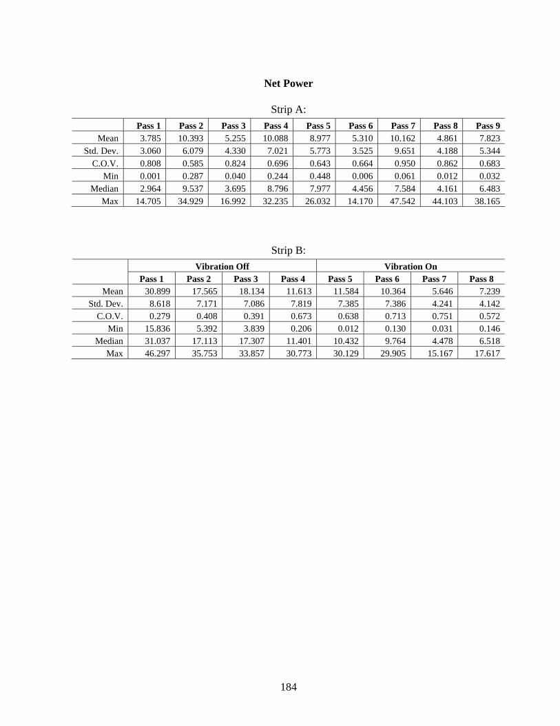
184

Net Power

Strip A: Pass 1 Pass 2 Pass 3 Pass 4 Pass 5 Pass 6 Pass 7 Pass 8 Pass 9

Mean 3.785 10.393 5.255 10.088 8.977 5.310 10.162 4.861 7.823 Std. Dev. 3.060 6.079 4.330 7.021 5.773 3.525 9.651 4.188 5.344

C.O.V. 0.808 0.585 0.824 0.696 0.643 0.664 0.950 0.862 0.683 Min 0.001 0.287 0.040 0.244 0.448 0.006 0.061 0.012 0.032

Median 2.964 9.537 3.695 8.796 7.977 4.456 7.584 4.161 6.483 Max 14.705 34.929 16.992 32.235 26.032 14.170 47.542 44.103 38.165

Strip B: Vibration Off Vibration On

Pass 1 Pass 2 Pass 3 Pass 4 Pass 5 Pass 6 Pass 7 Pass 8 Mean 30.899 17.565 18.134 11.613 11.584 10.364 5.646 7.239

Std. Dev. 8.618 7.171 7.086 7.819 7.385 7.386 4.241 4.142 C.O.V. 0.279 0.408 0.391 0.673 0.638 0.713 0.751 0.572

Min 15.836 5.392 3.839 0.206 0.012 0.130 0.031 0.146 Median 31.037 17.113 17.307 11.401 10.432 9.764 4.478 6.518

Max 46.297 35.753 33.857 30.773 30.129 29.905 15.167 17.617

III. Measured Soil Properties

A. Scatter Plots (Soil Properties vs. Number of Passes)

Strip A:

Dry Density by Number of Passes, Strip A Moisture Content by Number of Passes, Strip A

"' "' C)

"' ;! <

~ C)

~ ,... ~ :~ c: Q) C)

0 ~

<=' 0

~ C)

"' E Q)

00 E "' 0 0

~ (!) ::> "' <;; ·c;

"' 2: "' C)

"' "' 1.0 1.5 2.0 2.5 3.0 3.5 4.0 1.0 1.5 2.0 2.5 3.0 3.5 4.0

Number of Passes Number of Passes

Clegg Impact Value by Number of Passes, Strip A MDCP by Number of Passes, Strip A

C)

C) C)

"' Q) "' ::> (;;

> u C)

"' "' a. .§

Q_ C)

0 ~ 0 2:

"' C) "' Q) "' (3

C)

~

C)

1.0 1.5 2.0 2.5 3.0 3.5 4.0 1.0 1.5 2.0 2.5 3.0 3.5 4.0

Number of Passes Number of Passes

186

Strip B:


Strip A: Moisture Content (%):

Pass 1 2 3 4

Mean 27.77 26.85 27.77 27.77 St.Dev 2.46 3.85 2.46 2.46 COV 0.09 0.14 0.09 0.09 Max. 29.90 32.00 29.90 29.90 Median 28.15 26.15 28.15 28.15 Min. 23.60 22.30 23.60 23.60

187

Dry Density (KN/m3): Pass 1 2 3 4

Mean 12.39 13.23 12.81 13.49 St.Dev 1.31 0.53 0.77 0.79 COV 0.11 0.04 0.06 0.06 Max. 13.82 13.87 13.59 14.45 Median 12.01 13.19 13.16 13.49 Min. 10.97 12.58 11.65 12.29

Clegg Impact Value:

Pass 1 2 3 4 Mean 2.88 3.72 2.68 3.38 St.Dev 0.58 0.47 1.11 0.97 COV 0.20 0.13 0.42 0.29 Max. 3.40 4.20 3.70 4.50 Median 3.00 3.80 2.50 3.20 Min. 1.90 3.10 1.00 2.00

MDCP (mm/blow):

Pass 1 2 3 4 Mean 2.88 3.72 2.68 3.38 St.Dev 0.58 0.47 1.11 0.97 COV 0.20 0.13 0.42 0.29 Max. 3.40 4.20 3.70 4.50 Median 3.00 3.80 2.50 3.20

Strip B:

Moisture Content (%): Pass 1 2 3 4 6 8

Mean 25.43 22.35 21.96 21.27 21.85 22.06 St.Dev 1.81 1.62 1.64 1.85 1.13 1.52 COV 0.07 0.07 0.07 0.09 0.05 0.07 Max. 27.30 24.20 24.05 23.70 23.05 23.75 Median 25.45 21.80 22.20 21.20 22.30 22.10 Min. 23.15 20.85 20.15 18.80 20.10 19.95

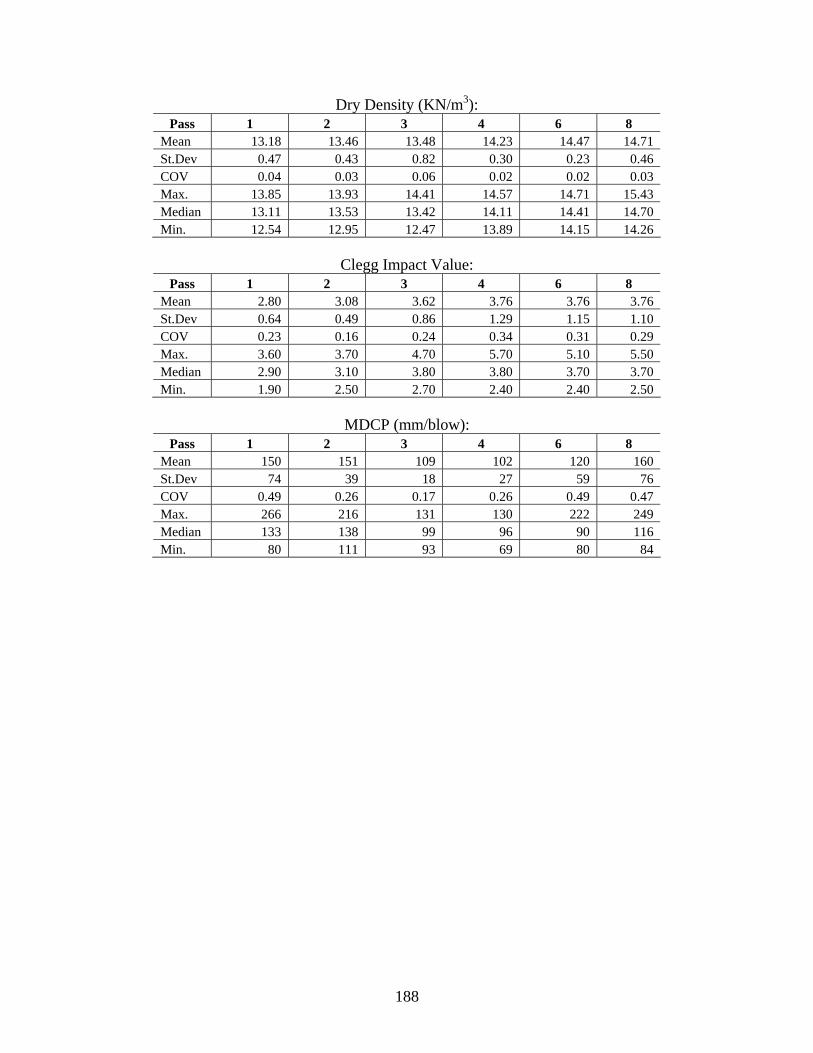
188

Dry Density (KN/m3): Pass 1 2 3 4 6 8

Mean 13.18 13.46 13.48 14.23 14.47 14.71 St.Dev 0.47 0.43 0.82 0.30 0.23 0.46 COV 0.04 0.03 0.06 0.02 0.02 0.03 Max. 13.85 13.93 14.41 14.57 14.71 15.43 Median 13.11 13.53 13.42 14.11 14.41 14.70 Min. 12.54 12.95 12.47 13.89 14.15 14.26

Clegg Impact Value:

Pass 1 2 3 4 6 8 Mean 2.80 3.08 3.62 3.76 3.76 3.76 St.Dev 0.64 0.49 0.86 1.29 1.15 1.10 COV 0.23 0.16 0.24 0.34 0.31 0.29 Max. 3.60 3.70 4.70 5.70 5.10 5.50 Median 2.90 3.10 3.80 3.80 3.70 3.70 Min. 1.90 2.50 2.70 2.40 2.40 2.50

MDCP (mm/blow):

Pass 1 2 3 4 6 8 Mean 150 151 109 102 120 160 St.Dev 74 39 18 27 59 76 COV 0.49 0.26 0.17 0.26 0.49 0.47 Max. 266 216 131 130 222 249 Median 133 138 99 96 90 116 Min. 80 111 93 69 80 84

field evaluation of compaction monitoring technology: phase i

Documents