fighting poverty: assessing the effect of guaranteed minimum
TRANSCRIPT

DI
SC
US
SI
ON
P
AP
ER
S
ER
IE
S
Forschungsinstitut zur Zukunft der ArbeitInstitute for the Study of Labor
Fighting Poverty: Assessing the Effect of Guaranteed Minimum Income Proposals in Québec
IZA DP No. 7283
March 2013
Nicholas-James ClavetJean-Yves DuclosGuy Lacroix

Fighting Poverty: Assessing the Effect of Guaranteed
Minimum Income Proposals in Québec
Nicholas-James Clavet CIRPÉE, Université Laval
Jean-Yves Duclos
CIRPÉE, CIRANO, Université Laval and IZA
Guy Lacroix
CIRPÉE, CIRANO, Université Laval and IZA
Discussion Paper No. 7283 March 2013
IZA
P.O. Box 7240 53072 Bonn
Germany
Phone: +49-228-3894-0 Fax: +49-228-3894-180
E-mail: [email protected]
Any opinions expressed here are those of the author(s) and not those of IZA. Research published in this series may include views on policy, but the institute itself takes no institutional policy positions. The IZA research network is committed to the IZA Guiding Principles of Research Integrity. The Institute for the Study of Labor (IZA) in Bonn is a local and virtual international research center and a place of communication between science, politics and business. IZA is an independent nonprofit organization supported by Deutsche Post Foundation. The center is associated with the University of Bonn and offers a stimulating research environment through its international network, workshops and conferences, data service, project support, research visits and doctoral program. IZA engages in (i) original and internationally competitive research in all fields of labor economics, (ii) development of policy concepts, and (iii) dissemination of research results and concepts to the interested public. IZA Discussion Papers often represent preliminary work and are circulated to encourage discussion. Citation of such a paper should account for its provisional character. A revised version may be available directly from the author.
IZA Discussion Paper No. 7283 March 2013
ABSTRACT
Fighting Poverty: Assessing the Effect of Guaranteed Minimum Income Proposals in Québec
This paper analyzes the impact of a recent recommendation made by Quebec’s Comité consultatif de lutte contre la pauvreté et l’exclusion sociale to guarantee every individual an income equal to 80% of Statistics Canada’s Market Basket Measure (MBM). Workers with earnings at least equivalent to 16 weekly hours at the minimum wage would be entitled to 100% of the MBM. We also investigate the impact of three alternative proposals: 1) a change in the above the hours cut-off from 16 to 30 hours; 2) a guaranteed income equal to 100% of the MBM, irrespective of earnings; 3) a 3$/hour conditional wage subsidy. To do this, we first estimate a structural labor supply model using the existing tax code and predict the labor supply of a representative sample of individuals based upon the parameter estimates of the model. Simulations show that the original recommendation would have strong negative impacts on participation rates of low-earners and that its cost would exceed $ 2 billion. Increasing the hours cut-off is predicted to have little impact beyond those of the original recommendation. Providing a guaranteed income equivalent to 100% of the MBM, on the other hand, would have a large impact. We find that contrary to what is usually assumed, guaranteed income schemes may increase the incidence of low-income rather than decrease it. JEL Classification: C25, D31, D63, H31, I30, J22 Keywords: Guaranteed Minimum Income, ex ante evaluation, labor market effects,
financial cost, poverty alleviation, public finance Corresponding author: Jean-Yves Duclos Department of economics Pavillon de Sève Université Laval Québec, QC, G1V 0A6 Canada E-mail: [email protected]
1 Introduction
Over the past fifteen years, the Government of Quebec has introduced a numberof relatively novel policies aimed at fighting poverty. The most comprehensiveinitiative has certainly been the enactment in 2002 of Bill 112, known as An Actto Combat Poverty and Social Exclusion. The Act is quite ambitious:
The object of this Act is to guide the Government of Québec and society asa whole towards a process of planning and implementing actions to combatpoverty, prevent its causes, reduce its effects on individuals and families,counter social exclusion, and strive towards a poverty-free Québec.
Such an Act is unique in North America; it also constitutes a significant politicalinnovation, if only because it makes poverty reduction an explicit and central policypriority. The Act also establishes A National Strategy to Combat Poverty and SocialExclusion and provides for the creation of an Anti-Poverty Fund (“Fonds québécoisd’initiatives sociales”). It has further instituted an advisory committee known asthe CCLP (“Comité consultatif de lutte contre la pauvreté et l’exclusion sociale”).The role of the CCLP is to advise the government on the planning, implementationand assessment of actions taken within the scope of the National Strategy. TheCCLP may also make recommendations and give opinions on government policiesthat may have a direct or indirect impact on poverty and social exclusion.
In this context, the CCLP published in 2009 a report containing a series of inter-esting and important recommendations on the means of ensuring that all Quebecershave incomes that enable them to meet their basic needs (Comité consultatif delutte contre la pauvreté et l’exclusion sociale 2009). Two of these recommenda-tions (to which we refer jointly as the “CCLP recommendation”) are the focus ofthe present paper. They are singled out because they naturally lend themselves toanalytical investigation and also because together they broadly amount to estab-lishing a guaranteed minimum income.
1

The purpose of this paper is thus to investigate the likely impact of the CCLPrecommendation on the employment and income of the residents of the Province ofQuebec. Naturally, the usual ex post approaches to program evaluation cannot berelied upon as the recommendation has not yet been implemented. Rather, we relyon what is known as ex ante evaluation in the literature. An ex ante evaluationinvolves simulating the impacts of hypothetical/new programs or forecasting theimpacts of existing programs in new contexts. Typically these evaluations dependon a structural estimation of the parameters of a model (Todd and Wolpin 2006)or on a reduced form model derived from a specific structural model.1 The ex anteevaluation of a program then uses these behavioural parameters to estimate by howmuch behaviour would be expected to change if the program were implemented.
Ex ante evaluations are particularly useful in a program development phase tomake informed decisions for extending the target population of an existing pro-gram. They also facilitate an optimal use of limited resources by ensuring thatgovernments make financial investments in programs that are likely to have a use-ful impact. These evaluations are helpful in considering implementation of newprograms and can also serve as complements to future ex post evaluations.
Ex ante evaluations differ from ex post evaluations in that the data are observedfor only the “untreated” population. In this case, the counterfactual to be es-timated is the set of outcomes for the population to be treated rather than forthe controls. The key identification condition in this approach boils down to theprogram having an impact only through individual budget constraints. This is pre-cisely why we focus on two specific “recommendations” made in the CCLP report:they both impact the individual budget constraints. To be more specific, the tworecommendations we investigate are the following (see recommendations 2 and 13in Comité consultatif de lutte contre la pauvreté et l’exclusion sociale 2009):
Recommendation 1 The CCLP recommends that, as a first step, baseline finan-cial support be set at 80% of (Statistics Canada’s) Market Basket Measure(MBM) for disposable income in municipalities with a population of fewerthan 30,000 inhabitants.
Recommendation 2 The CCLP recommends that individuals who work an aver-age of 16 weekly hours at the minimum wage have a disposable income thatis no lower than the above Market Basket Measure for disposable income inmunicipalities with a population of fewer than 30,000 inhabitants.
2
These recommendations (to which we refer jointly as the “CCLP recommendation”)are the main focus of the paper because they were proposed by a government ad-visory committee and have the potential to become official policy. We neverthelessinvestigate three variants of the CCLP recommendation:
1. Change the 80%-100% MBM cut-off from 16 hours per week to 30.
2. Raise the financial support to 100% of the MBM to everyone, irrespective ofhours of work.
3. Provide a 3$/hour subsidy to individuals who find a job and work at least 30hours per week.
The first variant makes the CCLP recommendation somewhat less generous. Itis equivalent to increasing the implicit tax rate on earnings. We will refer to thisvariant as “16-30 CO” in what follows. The second variant makes the CCLP rec-ommendation somewhat more generous because the guaranteed minimum incomeis independent of hours of work. It will be referred to as “100% MBM”. Finally, thethird variant, “AE-SSP”, borrows from Action Emploi and the SSP and proposesto investigate the impact of a conditional 3$/hour wage subsidy.
Our strategy consists estimating a structural labor supply model using a rep-resentative sample of Quebec residents and in which the budget constraints arebased upon the existing tax code. We next modify the budget constraints in ac-cordance with the above original and modified proposals and simulate their likelylong-term impact on employment and income using the parameter estimates of theeconometric model.
Our results show that the original CCLP recommendation would have a largenegative impact on hours of work and labor force participation — and mostly soamong low-income workers. In addition, the CCLP recommendation would berather costly. It would amount to additional outlays of the order of $ 2.2 billionsper year, of which 85% would be borne by the provincial government. Changingthe cut-off from 16 to 30 hours is predicted to have little impacts beyond those ofthe original recommendation. Providing a guaranteed income equivalent to 100%of the MBM would, however, have a large impact. The total program outlaywould amount to $ 3.7 billion, almost twice as much as for the original CCLPrecommendation. The behavioural reactions to the guaranteed minimum schemesare large enough so that more individuals end up with a lower income than in
3
the absence of those schemes. Only the AE-SSP scenario has an unambiguouslypositive impact on labor supply and income.
2 Policy, Data and Budget Constraints
2.1 Self-sufficiency and Employment
As stressed in its Policy Statement (Gouvernement du Québec 2002), the Govern-ment of Quebec considers employment to be the primary road to independence andoften the best way to combat poverty. The CCLP report and the government’sstatement are reminiscent of the debate on the competing objectives of providingsufficient income support to escape from material poverty while making work suffi-ciently attractive. Although social assistance typically provides low benefits (ofteninsufficient to escape material poverty by most standards), in some circumstancesit can represent an attractive alternative to low-paid work, especially for fami-lies with children. As stated by the Ontario Task Force on Income Security, “[a]modern income security system would expect and encourage individuals to assumepersonal responsibility for taking advantage of opportunities for engagement in theworkforce or in community life” (Task Force on Modernizing Income Security forWorking-Age Adults 2006, p.16). Longer-term receipt of social assistance can alsoreinforce poverty by deteriorating recipients’ employment skills and by loweringtheir aspirations and morale. Parental use of social assistance can further increasethe probability that their children will eventually be social assistance recipients(see Beaulieu et al. 2005 for evidence for Quebec).
Those governments that emphasize the importance of employment in combattingpoverty have typically implemented so-called “in-work benefits” to encourage work.The Earned Income Tax Credit in the United States, the Working Tax Credit inthe United Kingdom, and the Prime pour l’emploi in France are all examplesof policies that attempt to make work “pay”. A Canadian “Working Income TaxBenefit” (WITB) was introduced in March 2007 and consists of a relatively modestrefundable tax credit set to 20% of earned income up to $500 for individuals and$1,000 for families that is reduced by 15% of net income for individuals earningmore than $9,500 and families earning more than $14,500. The WITB aims atimproving the incentives to work for low-income Canadians and to lower the so-called “welfare wall”. Alternatives to these programs have also been proposed.
4
The Task Force on Modernizing Income Security for Working-Age Adults (2006)proposes to combine a Basic Refundable Tax Credit and a Working Income Benefitto all low-income working-age adults; such a program would offer a maximumbenefit of around $4,000 per year, which would begin to be clawed back at anincome level of around $5,000 per year and would be reduced to zero at income of$21,000 per year. The benefit would not be available to those without earnings;Saunders (2005) has recently supported such a scheme.
There is a large consensus in the literature that policies that increase the in-centives to work yield positive results (see,e.g. Keane 2011; Meghir and Phillips2010; Meyer 2010). Men are usually found to be somewhat less responsive thanwomen and single mothers to changes in the marginal tax rates. The decision ofwhether to take paid work is, however, quite sensitive to taxation and transfers forwomen and mothers in particular. Likewise, wage subsidies have also been foundto yield interesting results in terms of participation. In Canada, evidence fromstudies evaluating the Self-Sufficiency Project (SSP; see Card and Hyslop 2005,Card and Hyslop 2009, Brouillette and Lacroix 2010) has shown that single moth-ers can respond strongly to a generous wage subsidy. Similar results have beenfound in Quebec where the Action Emploi program closely mimics the SSP setup(Brouillette and Lacroix 2011).
Because labor supply appears to be sensitive to taxation and subsidies, it is usefulto investigate CCLP’s sweeping recommendation prior to their being implemented.Before we turn to formal modelling, we discuss the data upon which our analysis isbased and we graphically depict how the recommendation changes the individualbudget sets.
2.2 Sample Characteristics
Our analysis uses data primarily drawn from Statistics Canada’s Social PolicySimulation Database (SPSD/M) for 2004. SPSD/M provides a statistically repre-sentative database of individuals in their family context, with enough informationon each individual to compute taxes paid to and cash transfers received from gov-ernments. The main component of the database is the Survey of Labor and IncomeDynamics (SLID). Important variables that are unavailable in the SLID are im-puted by Statistics Canada using the Survey of Household Spending (SHS) andadministrative data. For the specific purposes of this study, additional variables
5
such as the net value of residence, the value of financial assets and the net worth ofthe vehicles owned have also been imputed using the Survey of Financial Securityof 2005 and Census data for 2001.2
Our sample omits individuals under 18 and over 65 years of age as well as full-timestudents and the disabled. Individuals reporting earnings from self-employmentand those working on average more than 70 hours per week are also excluded fromthe sample. Overall, the sample consists of 3,031 individuals. The labor supplymodel is estimated for three distinct sub-groups: single men, single women, andsingle mothers.3 Table 1 reports descriptive statistics on key variables included inthe econometric model. The patterns reported in the table are roughly consistentwith those found in the census data, e.g., single men are on average younger thanboth single women and single mothers. In addition, they tend to work more andearn a higher hourly wage rate. As a consequence, their earnings are also higherthan those of the other groups. Single mothers in our sample have on average1.72 children and 18% have preschoolers. The bottom panel of the table reportsthe sample weights of each sub-group along with their respective census weights toassess the representativeness of our sample. Single women and single mothers aresomewhat under-represented in our sample, whereas the opposite holds for singlemen. The discrepancies are partly attributable to relatively small sample sizes butalso to the fact that the algorithm used to generate our sample could not be strictlyapplied to the census data.
Table 1: Descriptive StatisticsVariables Single men Single women Single mothers
Mean Std-dev Mean Std-dev Mean Std-devAge 38.08 11.23 43.12 13.29 40.96 8.13Weekly hours of work 34.51 13.70 27.53 15.73 28.02 14.86Earnings ($1000) 43.42 66.23 23.42 34.86 21.45 16.84Non-labor earnings ($1000) 4.39 32.60 3.57 10.01 3.01 4.86Hourly wage rate ($) 16.51 5.14 14.50 4.09 14.75 3.99# Children 0–18 1.72 0.95Have preschool children 0.18 0.38Sample size 1 809 831 391Sample weights 385 962 265 469 100 669Census weights 327 246 291 841 186 966
2.3 Budget Constraints
In order to understand the likely impact of the CCLP recommendation and itsvariants, it is useful to depict graphically how they change the budget set of repre-sentative individuals. The budget sets are computed using the Canadian Tax and
6

0
4000
8000
12000
16000
20000
24000
10 20 30 40 50 60 70 80 0
0.05
0.1
0.15
0.2
0.25
0.3
0.35
Net
Ear
ning
s
Den
sity
of W
eekl
y H
ours
of W
ork
Weekly Hours of Work
CC
LP T
hres
hold
Density of Single MenDensity of Single Women
Budget set with CCLPCurrent budget set
(a) Single Males and Females With No Assets
0
4000
8000
12000
16000
20000
24000
10 20 30 40 50 60 70 80 0
0.05
0.1
0.15
0.2
0.25
0.3
0.35
Net
Ear
ning
s
Den
sity
of W
eekl
y H
ours
of W
ork
Weekly Hours of Work
CC
LP T
hres
hold
Weekly Hours of WorkCurrent budget set
Budget set with CCLP
(b) Single Mothers with Median Assets
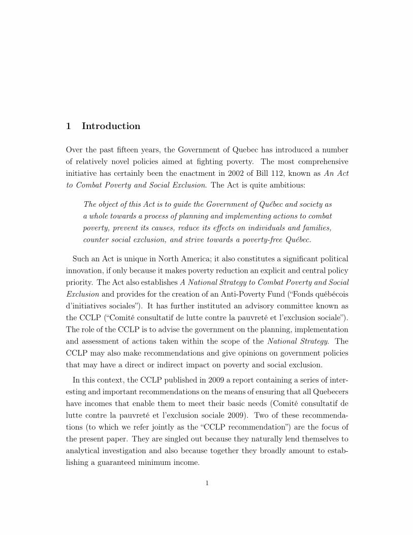
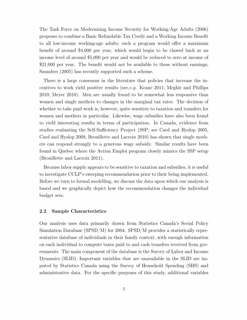
Figure 1: Budget Sets for Singles and Single Mothers, with and without CCLP benefits
Credit Simulator (CTaCS) developed by Milligan (2008). CTaCS simulates theCanadian personal income tax and transfer system (provincial and federal). Theprogram was slightly modified to take into account Quebec’s 2004 welfare bene-fits (Gouvernement du Québec 2004).4 For the sake of simplicity, we assume thatthe CCLP benefits would not be taxable at the federal level nor at the provinciallevel, and that no Employment Insurance or Quebec Pension Plan premia wouldbe levied against these benefits.
CCLP Budget Sets
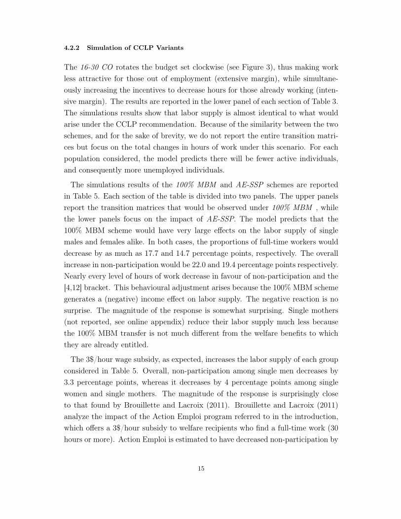
Figure 1(a) plots the yearly net earnings of single males and single females withno assets, while Figure 1(b) focuses on single mothers with median assets.5 Bothfigures are drawn under the assumption that workers earn the minimum wage andwork full-year at some weekly hours of work shown on the horizontal axis.
The dotted lines in both figures depict the budget sets under existing socialassistance programs. The solid lines are the budget sets derived from the CCLPrecommendation. The figures also plot the (weighted) densities of work hoursbased on our sample data. In both figures, the densities peak at approximately40 hours, although single mothers have a bimodal distribution with another peekat 30 weekly hours of work. The hours distribution highlights the fact that themajority of singles would have a strong incentive to reduce their hours of work.Even those whose earnings are higher than the cut-off point could still prefer towork less and earn less than they currently do.
Figure 1(a) focuses on single men and women. The budget set is identical for
7
0
1
2
3
4
5
6
7
8
10 20 30 40 50 60 70 80 0
1
2
3
4
5
6
7
8
Net
Hou
rly W
age
Rat
e
Net
Hou
rly W
age
Rat
e
Weekly Hours of Work
Without CCLPWith CCLP
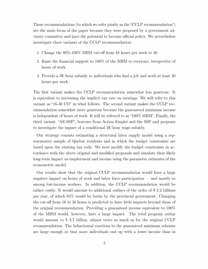
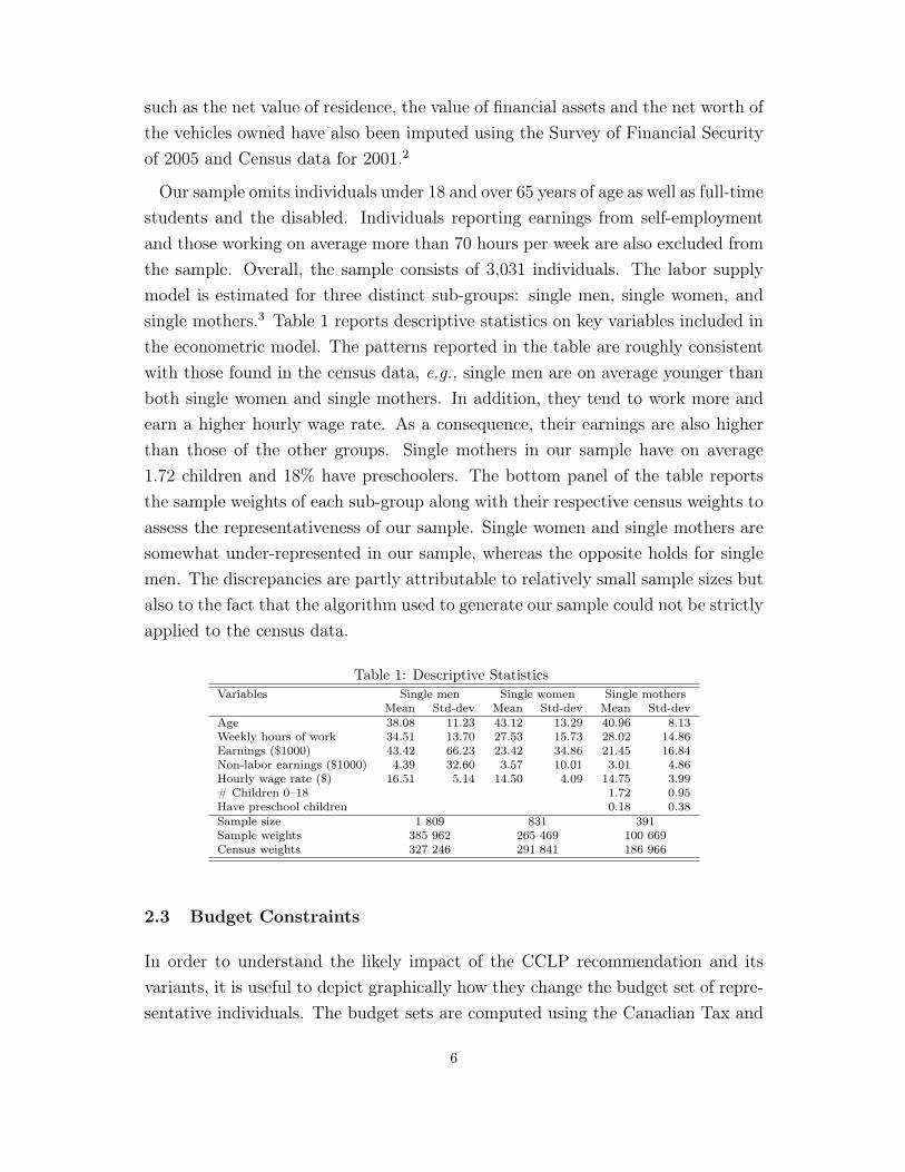
Figure 2: Net Hourly Wage Rate, Minimum Wage Worker, No Assets
both groups because it is drawn under the same assumptions (minimum wage, noassets, etc.). Notice first that inactive individuals would gain under the CCLPrecommendation. Indeed, they would receive a transfer equivalent to 80% of theMBM which is substantially more than the welfare benefits that prevailed in 2004.As they start working, their net earnings increase slowly because government trans-fers decrease fast. As they reach 16 hours per week, workers face an implicit taxrate of 100%.6 Beyond 32 weekly hours of work they are no longer entitled to thetransfer and they face the standard tax system. Under the existing system, netearnings increase faster than under the CCLP recommendation at first due to theearnings disregard in the determination of welfare benefits. A plateau is reached asearly as 7 hours of work per week because welfare benefits are taxed at an implicitrate of 100% beyond the corresponding earnings.
Figure 1(b) depicts the budget sets and the distribution of weekly hours of workof single mothers with median-level net assets and earning the minimum wage rate.Under the current welfare regime their monthly benefits are relatively low becausethey are means-tested. Under the CCLP regime, single mothers would enjoy aconsiderable increase in earnings.
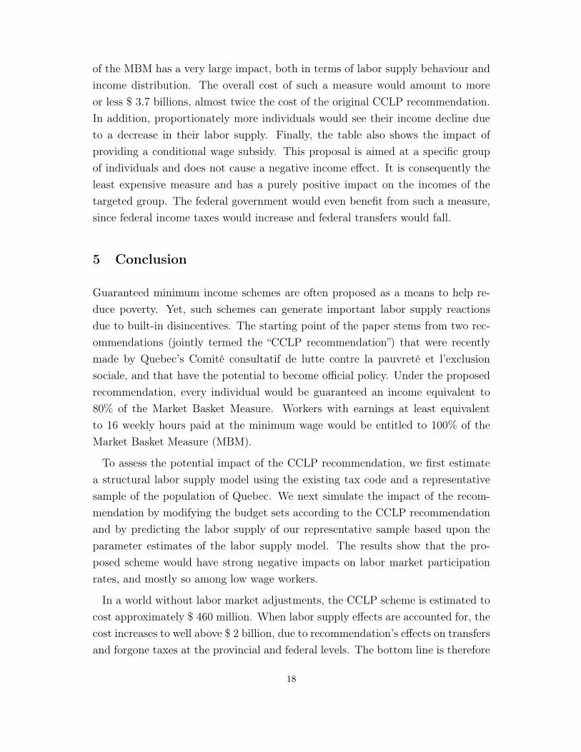
To gain a better understanding of the implicit incentive effects in both the CCLPand the status quo worlds, Figure 2 sketches the net hourly wage rate a single femaleearning the gross minimum wage and with no assets would enjoy as she increasesher weekly hours of work. In the current world, the income disregard in the welfare
8
system ensures a recipient’s earnings are not taxed away at low hours of work. Shethus enjoys a net wage rate of $7.45/hour. As her earnings increase beyond thedisregard, every additional dollar of earnings decreases her welfare benefits by onedollar. She thus earns a net wage rate of $0/hour. Once her earnings completelyexhaust her benefits, she starts paying income taxes and thus enjoys a net wagerate of about $6/hour. Finally, as her earnings increase beyond the first incometax bracket, she starts paying yet more taxes and works for a net wage rate ofabout $5/hour as a result.
In the CCLP world, the first hour of work increases earnings by as little as $2.91because the transfer received from the government decreases at a constant ratebetween 80% of the MBM at zero hours of work and 100% of the MBM at 16hours of work. Subsequently, as she works beyond 16 hours of work per week, shereceives a net wage rate of $0/hour. Only once she reaches 32 hours per week isher net wage rate again positive. This is because her earnings at 32 hours per weekare just equal to 100% of the MBM. Working in excess of 32 hours per week bringsher beyond the threshold and she no longer receives any transfer. Her earnings arethen large enough for her to pay income taxes.
The CCLP recommendation does not remove the “welfare trap” per se. Theysimply shift it rightwardly and as a consequence changes the incentive effects atlow hours of work.
Variants of CCLP Budget Sets
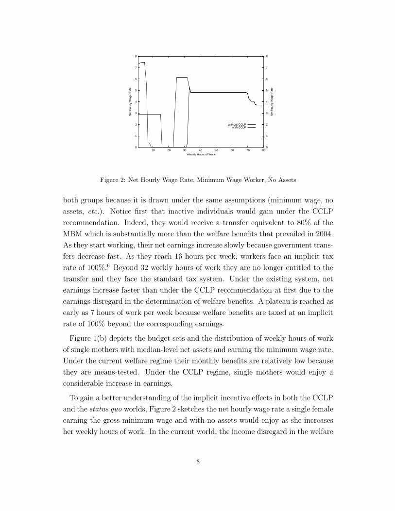
The 16-30 CO and AE-SSP variants are based upon recent policies that wereeither implemented in Québec or were part of demonstration projects conductedin British Columbia. Indeed, both the Self-Sufficiency Project (SSP, in BritishColumbia) and the Action Emploi program (AE, in Québec) required welfare par-ticipants to work at least 30 hours per week to qualify for an income subsidy. TheAE program provided a 3$/hour subsidy whereas the SSP project was somewhatmore generous.7 The 100% MBM corresponds more closely to what is usuallythought of as a universal guaranteed income.
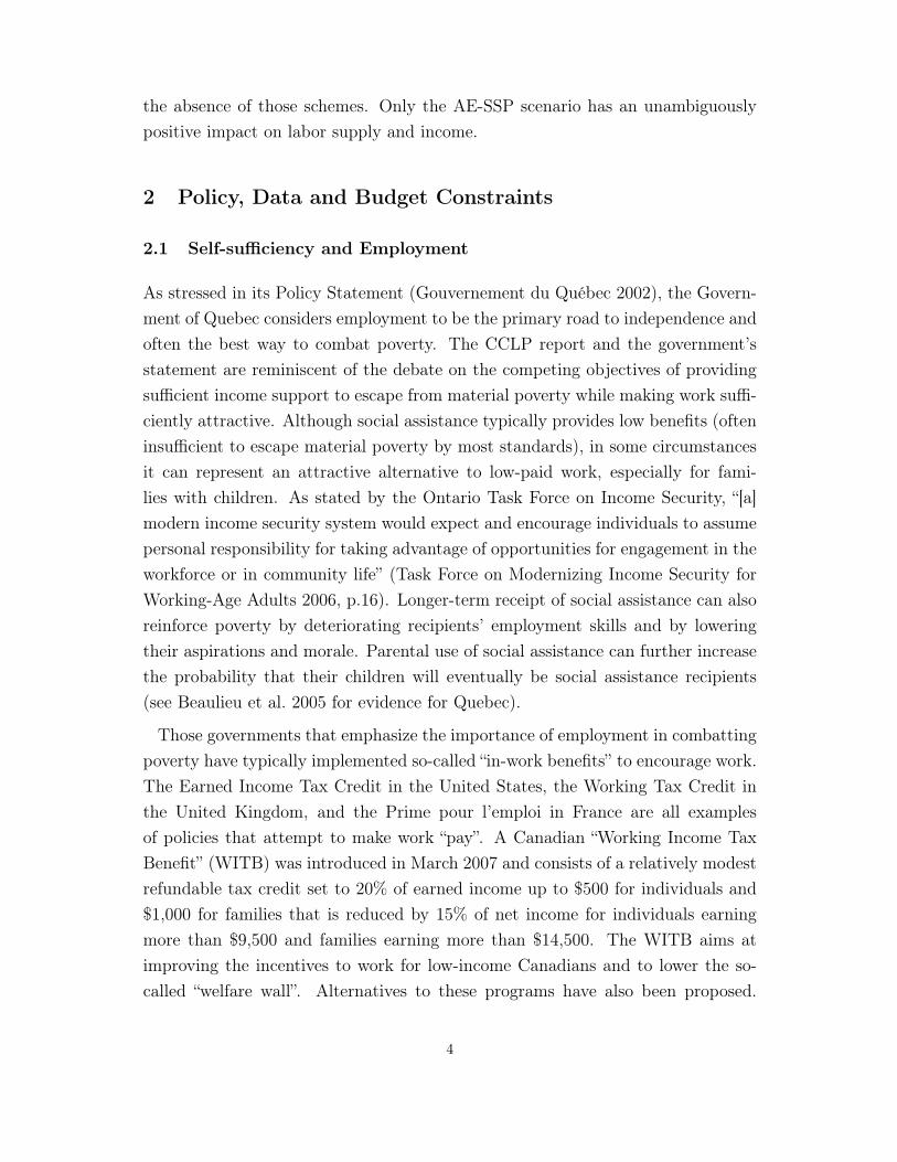
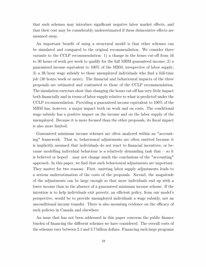
Figure 3 illustrates the budget sets of the CCLP recommendation along with thethree variants we consider. The figure is drawn for single mothers with medianasset values (the hours distribution is not depicted for ease of reading).
As before the solid line represents the current welfare system. The CCLP recom-mendation corresponds to the budget set that originates at 13,573$ and peaks at
9
0
4000
8000
12000
16000
20000
5 10 15 20 25 30 35 40 45 50
Net
Ear
ning
s
Weekly Hours of Work
CC
LP T
hres
hold
= 1
6
CC
LP T
hres
hold
= 3
0
CCLP with Threshold at 16 hours
CCLP with Threshold at 30 hours
CCLP with 100% MBM16967
13573
3$/hour subsid
y
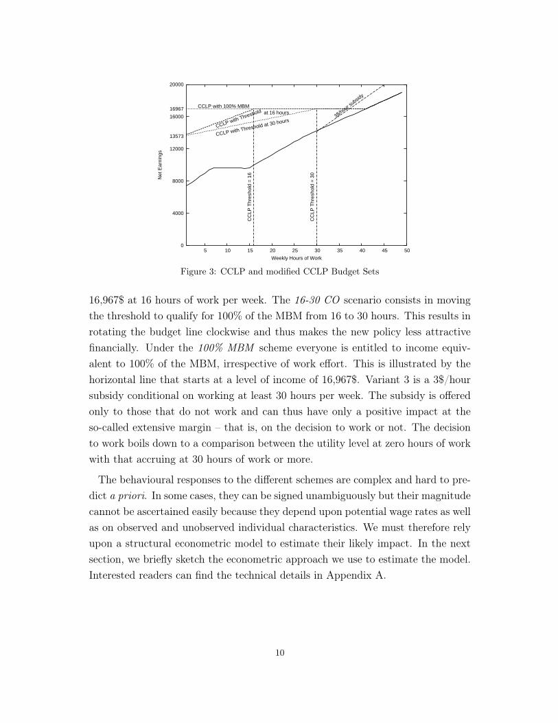
Figure 3: CCLP and modified CCLP Budget Sets
16,967$ at 16 hours of work per week. The 16-30 CO scenario consists in movingthe threshold to qualify for 100% of the MBM from 16 to 30 hours. This results inrotating the budget line clockwise and thus makes the new policy less attractivefinancially. Under the 100% MBM scheme everyone is entitled to income equiv-alent to 100% of the MBM, irrespective of work effort. This is illustrated by thehorizontal line that starts at a level of income of 16,967$. Variant 3 is a 3$/hoursubsidy conditional on working at least 30 hours per week. The subsidy is offeredonly to those that do not work and can thus have only a positive impact at theso-called extensive margin – that is, on the decision to work or not. The decisionto work boils down to a comparison between the utility level at zero hours of workwith that accruing at 30 hours of work or more.
The behavioural responses to the different schemes are complex and hard to pre-dict a priori. In some cases, they can be signed unambiguously but their magnitudecannot be ascertained easily because they depend upon potential wage rates as wellas on observed and unobserved individual characteristics. We must therefore relyupon a structural econometric model to estimate their likely impact. In the nextsection, we briefly sketch the econometric approach we use to estimate the model.Interested readers can find the technical details in Appendix A.
10
3 Econometric Model
Individuals are assumed to maximize a well-behaved utility function defined overleisure, l, and net income, y, with respect to time and income constraints:
max U i(li, yi) s.t. yi ≤ yi(li, w) and li ≤ T, (3.1)
where index i corresponds to a specific level of leisure defined as li = T − hi,where T = 80 is the time endowment, and where hi is weekly hours of work.8 Netincome equals earnings, whi, plus exogenous non-labor income, N , and governmenttransfers, B, less income taxes, T (Keane and Moffitt 1998):
yi(hi) = whi +N +B(whi, N,X)− T (whi, N,X), (3.2)
where X is a vector of demographic variables and w is the hourly wage rate. Fol-lowing convention, we assume that preferences can be approximated by a translogutility function. Heterogeneity in preferences is accounted for by conditioning theutility function, equation (3.1), on age, number of children in the household andpresence of preschoolers (single mother households).
Preference for leisure is also allowed to vary with unobserved characteristics. Thelatter are proxied by a random component that is assumed to be independentlyand identically distributed as a normal random variate. In addition, optimizationerrors are introduced into the utility function through another random componentthat is assumed to follow a Type-I extreme value distribution. This assumption ismade to allow for the possibility that the individual optimal choice of labor supplymay not correspond exactly to the discrete choices we specify in the model.
Finally, the literature on discrete labor supply models has generally found thatthe above model tends to under predict the number of individuals with h = 0
or h = 40. This will occur if the “fixed costs” associated with work (commuting,daycare, etc.) are not accounted for explicitly (see, e.g. Cogan 1981). These costsare difficult to measure but may be proxied by demographic variables. To accountfor bunching at 40 hours of work, we introduce in the utility function a dummyindicator that is equal to one if h = 40. The parameter associated with this dummyvariable will be positive if individuals value working that many hours and will benegative otherwise.
Given the above assumptions, it can be shown that the probability of working
11
hi hours of work per week is given by:
Pr[hi]=
∫exp (U i (li, yi) |υ)∑pj=1 exp (U
j (lj, yj) |υ)φ (υ) dυ, (3.3)
where φ is the normal density function of the unobserved preferences, υ. The ratioof exponential functions derives from assuming that the optimization errors followa Type-I extreme value distribution.
4 Estimation and Simulation Results
4.1 Estimation Results
The parameter estimates of the labor supply model of the three samples are pre-sented in Table 2. The parameters for the three samples are compatible with therequired quasi-concavity of the preferences, either globally or locally9: this is thecase for 100 % of single males and females and for 94.37 % of single mothers.Furthermore, net income is found to be a normal good for 100% of single females,98.19% of single mothers, and 96.47% of single males.10 It thus appears that, forthe majority of the individuals in our samples, hours of work can legitimately berepresented as the outcome of the maximization of utility under a budget con-straint.
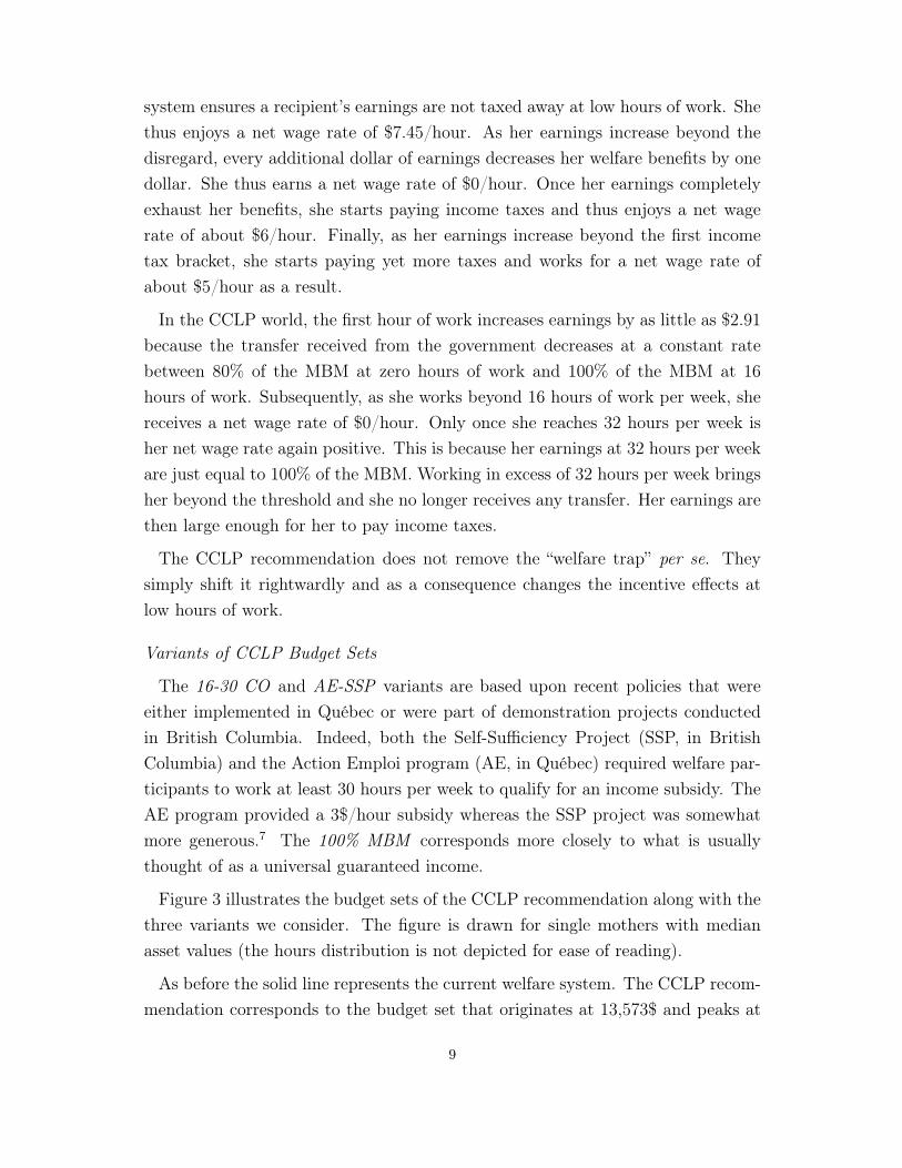
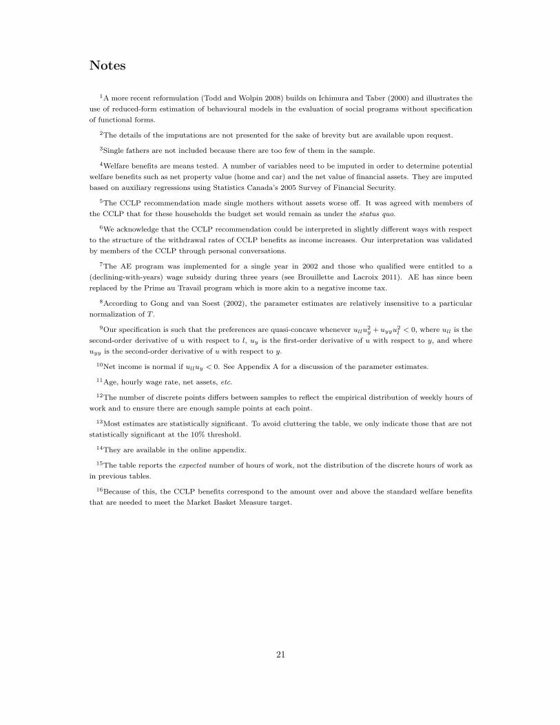
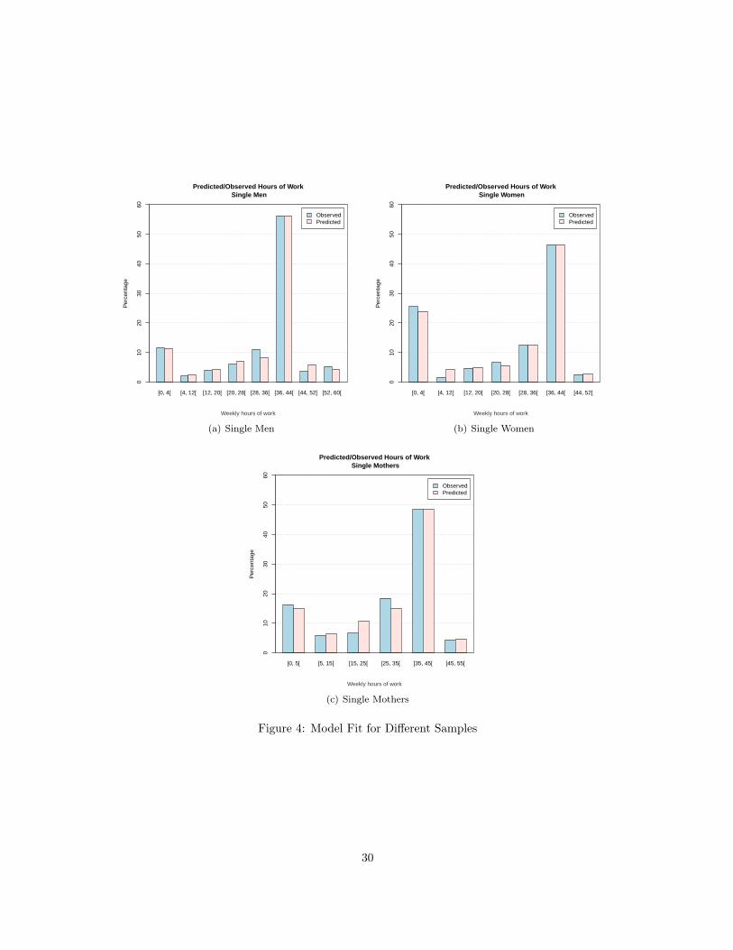
As a check on the overall fit of the model, we report observed and predicted dis-tributions of hours of work for the three samples separately in Figures 4(a)– 4(c).For each individual we compute the budget constraint based upon his/her char-acteristics.11 Next, we compute the utility associated with each discrete point ofhis/her budget constraint.12 The discrete point that yields the highest utility levelis then selected. The figures show that the model does a good job at predictingobserved outcomes. Indeed, the differences between observed and predicted choicesare small for each sample. In particular, the fit at zero [0,4[ and at [36,44[ and[35,45[ is almost perfect. Since the parameter estimates for the three samples areconsistent with a priori expectations and since nearly all individuals behave con-sistently with basic economic theory, we proceed to simulate the expected impactof the CCLP recommendation and of its variants with some confidence.
12

4.2 Simulation Results
The simulation exercise follows the strategy that was outlined in the previoussection. Individual budget sets are computed in accordance with the proposalsand based upon individual characteristics using CTaCS. Net income is computedfor each discrete point of the budget constraint. Finally, the utility level of eachpoint is computed and the one that yields the highest utility is selected (takinginto account the distribution of the different random terms).
4.2.1 Simulation of the CCLP recommendation
The upper panel of each section of Table 3 reports the impact on weekly hours ofwork of the CCLP recommendation. The 2004’s hours distribution is presented inthe last column of the table. Thus, for example, 11.63% of single men worked be-tween [0,4[ hours per week in 2004, and hours as many as 56.24% worked between[36,44[ hours per week. The hours distribution following the CCLP recommenda-tion is shown at the bottom of the upper panel of each section of Table 3. Hence,after the reform, 25.34% of single men would work between [0,4[ hours per week.
The expected hours distribution following the implementation of the recommen-dation is reported column-wise. The matrices thus decompose the total change inthe hours distribution into its different components. Numbers above the diagonalcorrespond to an increase (in percentage points) in weekly hours of work followingthe implementation of the CCLP recommendation, whereas the converse holds fornumbers below the diagonal.
For single men, a comparison between the diagonal elements with those of therightmost column reveals an important change in the hours distribution: the shareof workers reporting between 36 and 44 hours per week would decrease from 56.24%to 43.85%.13 For these workers, the decrease in full-time work would translateinto a larger share of non-participation (+9.98% in the [0,4[ hours bracket) and anincrease in the [4,12[ bracket (+1.85%). The difference in hours of work is reportedin the line entitled "Change". There we see that the the CCLP recommendationwould increase overall non-participation by 13.77 percentage points. Basically nochange is reported above the diagonal of the matrix. This is not surprising giventhat the CCLP recommendation offers little incentive to increase weekly hours ofwork.
13
The results for single women are very similar to those of single men except forthe fact that the changes in the hours of work distribution is more evenly spreadout. The overall increases in the [0,4[ and [4,12[ brackets (+12.64% and +1.93%,respectively) are associated with overall decreases in the [28,36[ and [36,44[ brackets(-2.68% and -10.69%, respectively). Just as in the above section of Table 3, verylittle is reported above the diagonal, and thus the CCLP’s recommendation ispredicted to have a significant negative impact on the labor supply of single females.
The simulations for single mothers are not reported for the sake of brevity.14
They show that the changes in the hours distribution are small and that none isstatistically significant, save for the [35,45[ bracket. This is not surprising giventhat only single mothers who have significant assets are predicted to be impactedby the recommendation. For the [35,45[ bracket, the share of full-time work ispredicted to decrease by 4.34 percentage points, much less than what is predictedfor single males and females. This is because although the majority of singlemothers (80%) in our sample have net positive assets, in only 45% of cases arethese assets large enough to decrease single mothers’ entitlement to social welfarebenefits. In addition, only 37% of the single mothers in our sample would beentitled to yearly CCLP benefits larger than 100$.
Table 4 goes one step further and reports the impact of the recommendation onthe expected weekly hours of work with respect to percentiles of net earnings.15 Italso distinguishes between the intensive margin, i.e. the impact on hours of workconditionally on working, and the extensive margin, i.e. the impact on participa-tion per se. The table reveals a number of interesting results. To start with, mostof the behavioural adjustments occur at the extensive margin, as shown in the firstcolumn. These results are entirely consistent with the recent literature on incometaxes and labor supply (see, e.g., Blundell 2000, Eissa and Hoynes 2006, Meyer2002). Thus, conditional on working, individuals decrease their weekly hours ofwork very little. Many choose, however, to stop working altogether. This responsevaries considerably with net earnings. According to Table 4, individuals in the bot-tom 10 and 25 income percentiles react most in percentage terms, while those inthe upper percentiles react less, especially at the intensive margin. All behaviouraladjustments at both the intensive and extensive margins are statistically differentfrom zero.
14
4.2.2 Simulation of CCLP Variants
The 16-30 CO rotates the budget set clockwise (see Figure 3), thus making workless attractive for those out of employment (extensive margin), while simultane-ously increasing the incentives to decrease hours for those already working (inten-sive margin). The results are reported in the lower panel of each section of Table 3.The simulations results show that labor supply is almost identical to what wouldarise under the CCLP recommendation. Because of the similarity between the twoschemes, and for the sake of brevity, we do not report the entire transition matri-ces but focus on the total changes in hours of work under this scenario. For eachpopulation considered, the model predicts there will be fewer active individuals,and consequently more unemployed individuals.
The simulations results of the 100% MBM and AE-SSP schemes are reportedin Table 5. Each section of the table is divided into two panels. The upper panelsreport the transition matrices that would be observed under 100% MBM , whilethe lower panels focus on the impact of AE-SSP. The model predicts that the100% MBM scheme would have very large effects on the labor supply of singlemales and females alike. In both cases, the proportions of full-time workers woulddecrease by as much as 17.7 and 14.7 percentage points, respectively. The overallincrease in non-participation would be 22.0 and 19.4 percentage points respectively.Nearly every level of hours of work decrease in favour of non-participation and the[4,12] bracket. This behavioural adjustment arises because the 100% MBM schemegenerates a (negative) income effect on labor supply. The negative reaction is nosurprise. The magnitude of the response is somewhat surprising. Single mothers(not reported, see online appendix) reduce their labor supply much less becausethe 100% MBM transfer is not much different from the welfare benefits to whichthey are already entitled.
The 3$/hour wage subsidy, as expected, increases the labor supply of each groupconsidered in Table 5. Overall, non-participation among single men decreases by3.3 percentage points, whereas it decreases by 4 percentage points among singlewomen and single mothers. The magnitude of the response is surprisingly closeto that found by Brouillette and Lacroix (2011). Brouillette and Lacroix (2011)analyze the impact of the Action Emploi program referred to in the introduction,which offers a 3$/hour subsidy to welfare recipients who find a full-time work (30hours or more). Action Emploi is estimated to have decreased non-participation by
15

single mothers by anywhere between 4.2 and 6.6 percentage points. Our structuralmodel generates very similar results despite the fact that it is an ex ante exerciseand despite the fact that it rests upon an entirely different set of assumptions,model and data. The fact that this structural model is able to replicate well thefindings of Brouillette and Lacroix (2011) would seem to provide further credenceto our simulations.
4.3 The Cost of the CCLP recommendation
All in all, our simulation results show that single males and females would reactstrongly to the CCLP recommendation. Furthermore, our simulations also showthat those that would respond most are precisely those that have the lowest currentearnings. The sharp decreases in participation rates and ensuing decreases inincome taxes, coupled with sizeable outlays, may make the CCLP recommendationcostly. We now turn to this issue.
In addition to the CCLP benefits per se, the CCLP costs to the federal andprovincial governments must take into account changes in income taxes, transfers,social assistance benefits, Quebec Pension Plan and Employment Insurance pre-miums, etc. These changes are computed under two different scenarios. In thefirst, the accounting scenario, we assume that the labor supply response follow-ing the implementation of the CCLP recommendation is null. In the second, thebehavioural scenario, we allow for such a response. In both cases, we start bycomputing the taxes and transfers of each individual in our sample based on theirobserved labor supply. We next modify the budget constraints according to theCCLP recommendation and compute the taxes and transfers again. The differ-ences are then multiplied by the individual sample weights to obtain an aggregateestimate of the cost of the two scenarios.
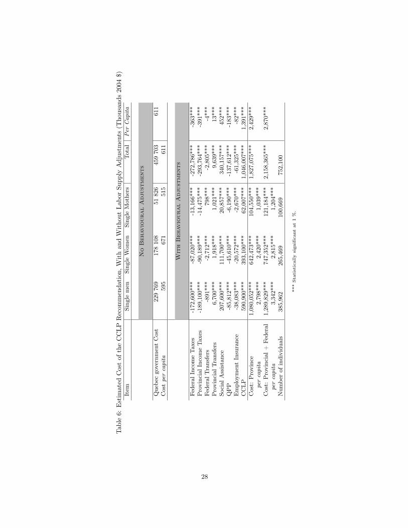
Table 6 reports the detailed costs associated with both scenarios. The upper-half panel concerns the accounting scenario. Recall that we assume that the CCLPbenefits would not be taxable at the federal nor at the provincial levels, and that noEmployment Insurance or Quebec Pension Plan premiums would be levied againstthose benefits.16 In the case in which federal taxes would be levied against theCCLP benefits, the latter would have to be increased so that the net income ac-cruing to the individual would meet the CCLP income objectives. Those additionalCCLP expenses would represent an additional cost for the provincial government
16

and additional revenues for the federal government. From a joint provincial-federalfiscal perspective, the overall cost of the CCLP recommendation would, however,not be altered were the benefits to be taxed at the federal level.
The upper panel of Table 6 represents the additional cost the provincial govern-ment would have to bear in order to implement the CCLP’s recommendation. Theamounts are in addition to the standard welfare benefits. Many more individu-als would receive CCLP benefits than there are welfare recipients. Consequently,the additional amounts are sizeable. The per capita cost of the recommendationwould vary between $500 and $700 per individual, and are slightly larger for singlewomen.
The lower panel of Table 6 reports the results of the behavioural scenario. Federaland provincial income taxes decrease because many individual decrease their laborsupply in response to the CCLP benefits. Social assistance payments increase forthe same reason: those who reduce their hours of work substantially or completelyoften become entitled to welfare benefits. The CCLP payments thus correspondto the additional outlays the government must bear to meet the requirementsof the CCLP’s recommendation. They are larger than in the accounting scenariobecause many individuals are expected to decrease their labor supply sufficiently toqualify for the benefits. The overall cost of the recommendation is predicted to beimportant: approximately $2,870 per individual, which is more than four times theper capita cost of the accounting scenario. The total CCLP costs would then be ofthe order of $2.2 billion, 85% of which would be borne by the provincial government.The remaining $331 million would be borne by the federal government, $286 millionof which through a decrease in personal income tax revenue.
Table 7 reports the overall cost of the CCLP recommendation along with those of16-30 CO, 100% MBM and AE-SSP. We also indicate for each sample and for eachcase the proportions of individuals whose net income would increase, decrease orremain constant. Were the CCLP’s recommendation implemented, the simulationsindicate that slightly more would individuals would see their income decrease. Thisresult is entirely driven by behavioural adjustments: non-participants benefit froman increased income whereas those who decrease their labor supply do so at thecost of lower income. As mentioned above, increasing the hours cut-off from 16to 30 hours of work is predicted to have little behavioural impact. Consequently,the costs associated with this proposal are almost identical to those of the originalCCLP recommendation. On the other hand, providing each individual with 100%
17
of the MBM has a very large impact, both in terms of labor supply behaviour andincome distribution. The overall cost of such a measure would amount to moreor less $ 3.7 billions, almost twice the cost of the original CCLP recommendation.In addition, proportionately more individuals would see their income decline dueto a decrease in their labor supply. Finally, the table also shows the impact ofproviding a conditional wage subsidy. This proposal is aimed at a specific groupof individuals and does not cause a negative income effect. It is consequently theleast expensive measure and has a purely positive impact on the incomes of thetargeted group. The federal government would even benefit from such a measure,since federal income taxes would increase and federal transfers would fall.
5 Conclusion
Guaranteed minimum income schemes are often proposed as a means to help re-duce poverty. Yet, such schemes can generate important labor supply reactionsdue to built-in disincentives. The starting point of the paper stems from two rec-ommendations (jointly termed the “CCLP recommendation”) that were recentlymade by Quebec’s Comité consultatif de lutte contre la pauvreté et l’exclusionsociale, and that have the potential to become official policy. Under the proposedrecommendation, every individual would be guaranteed an income equivalent to80% of the Market Basket Measure. Workers with earnings at least equivalentto 16 weekly hours paid at the minimum wage would be entitled to 100% of theMarket Basket Measure (MBM).
To assess the potential impact of the CCLP recommendation, we first estimatea structural labor supply model using the existing tax code and a representativesample of the population of Quebec. We next simulate the impact of the recom-mendation by modifying the budget sets according to the CCLP recommendationand by predicting the labor supply of our representative sample based upon theparameter estimates of the labor supply model. The results show that the pro-posed scheme would have strong negative impacts on labor market participationrates, and mostly so among low wage workers.
In a world without labor market adjustments, the CCLP scheme is estimated tocost approximately $ 460 million. When labor supply effects are accounted for, thecost increases to well above $ 2 billion, due to recommendation’s effects on transfersand forgone taxes at the provincial and federal levels. The bottom line is therefore
18
that such schemes may introduce significant negative labor market effects, andthat their cost may be considerably underestimated if these disincentive effects areassumed away.
An important benefit of using a structural model is that other schemes canbe simulated and compared to the original recommendation. We consider threevariants to the CCLP recommendation: 1) a change in the hours cut-off from 16to 30 hours of work per week to qualify for the full MBM guaranteed income; 2) aguaranteed income equivalent to 100% of the MBM, irrespective of labor supply;3) a 3$/hour wage subsidy to those unemployed individuals who find a full-timejob (30 hours/week or more). The financial and behavioural impacts of the threeproposals are estimated and contrasted to those of the CCLP recommendation.The simulation exercises show that changing the hours cut-off has very little impactboth financially and in terms of labor supply relative to what is predicted under theCCLP recommendation. Providing a guaranteed income equivalent to 100% of theMBM has, however, a major impact both on work and on costs. The conditionalwage subsidy has a positive impact on the income and on the labor supply of theunemployed. Because it is more focused than the other proposals, its fiscal impactis also more limited.
Guaranteed minimum income schemes are often analyzed within an "account-ing" framework. That is, behavioural adjustments are often omitted because itis implicitly assumed that individuals do not react to financial incentives, or be-cause modelling individual behaviour is a relatively demanding task that – so itis believed or hoped – may not change much the conclusions of the "accounting"approach. In this paper, we find that such behavioural adjustments are important.They matter for two reasons. First, omitting labor supply adjustments leads toa serious underestimation of the costs of the proposals. Second, the magnitudeof the adjustments can be large enough so that more individuals end up with alower income than in the absence of a guaranteed minimum income scheme. If theintention is to help individuals exit poverty, an efficient policy, from our model’sperspective, would be to provide unemployed individuals a wage subsidy, not anunconditional income transfer. There is also mounting evidence on the efficacy ofsuch policies in Canada and elsewhere.
An issue that has not been addressed in this paper concerns the public financeburden of financing the different schemes we have considered. The overall costs ofthe schemes vary between 2.1 and 3.7 billion dollars. Financing such large programs
19

would necessarily require that taxes be raised. This would in all likelihood lead toyet larger labor supply adjustments. The costs reported in this paper are thereforeprobably conservative. We leave this issue open for future research.
20
Notes
1A more recent reformulation (Todd and Wolpin 2008) builds on Ichimura and Taber (2000) and illustrates theuse of reduced-form estimation of behavioural models in the evaluation of social programs without specificationof functional forms.
2The details of the imputations are not presented for the sake of brevity but are available upon request.
3Single fathers are not included because there are too few of them in the sample.
4Welfare benefits are means tested. A number of variables need to be imputed in order to determine potentialwelfare benefits such as net property value (home and car) and the net value of financial assets. They are imputedbased on auxiliary regressions using Statistics Canada’s 2005 Survey of Financial Security.
5The CCLP recommendation made single mothers without assets worse off. It was agreed with members ofthe CCLP that for these households the budget set would remain as under the status quo.
6We acknowledge that the CCLP recommendation could be interpreted in slightly different ways with respectto the structure of the withdrawal rates of CCLP benefits as income increases. Our interpretation was validatedby members of the CCLP through personal conversations.
7The AE program was implemented for a single year in 2002 and those who qualified were entitled to a(declining-with-years) wage subsidy during three years (see Brouillette and Lacroix 2011). AE has since beenreplaced by the Prime au Travail program which is more akin to a negative income tax.
8According to Gong and van Soest (2002), the parameter estimates are relatively insensitive to a particularnormalization of T .
9Our specification is such that the preferences are quasi-concave whenever ullu2y + uyyu2
l < 0, where ull is thesecond-order derivative of u with respect to l, uy is the first-order derivative of u with respect to y, and whereuyy is the second-order derivative of u with respect to y.
10Net income is normal if ulluy < 0. See Appendix A for a discussion of the parameter estimates.
11Age, hourly wage rate, net assets, etc.
12The number of discrete points differs between samples to reflect the empirical distribution of weekly hours ofwork and to ensure there are enough sample points at each point.
13Most estimates are statistically significant. To avoid cluttering the table, we only indicate those that are notstatistically significant at the 10% threshold.
14They are available in the online appendix.
15The table reports the expected number of hours of work, not the distribution of the discrete hours of work asin previous tables.
16Because of this, the CCLP benefits correspond to the amount over and above the standard welfare benefitsthat are needed to meet the Market Basket Measure target.
21
References
Beaulieu, Nicolas, J.-Y. Duclos, Bernard Fortin, and Manon Rouleau (2005) ‘In-tergenerational reliance on social assistance: Evidence from canada.’ Journal ofPopulation Economics 18(3), 539–562
Blundell, Richard (2000) ‘Work Incentives and “In-Work” Benefit Reforms : AReview.’ Oxford Review of Economic Policy 16(1), 27–44
Brouillette, Dany, and Guy Lacroix (2010) ‘Heterogeneous treatment and self-selection in a wage subsidy experiment.’ Journal of Public Economics 94, 479 –492
(2011) ‘Assessing the impact of a wage subsidy for single parents on socialassistance.’ Canadian Journal of Economics/Revue canadienne d’économique44(4), 1195–1221
Card, David, and Dean R. Hyslop (2005) ‘Estimating the effects of a time-limitedearnings subsidy for welfare-leavers.’ Econometrica 73(6), 1723–1770
Card, David, and Dean R. Hyslop (2009) ‘The dynamic effects of an earningssubsidy for long-term welfare recipients: Evidence from the self sufficiency projectapplicant experiment.’ Journal of Econometrics 153(1), 1–20
Cogan, J. (1981) ‘Fixed cost and labour supply.’ Econometrica 49, 945–964
Comité consultatif de lutte contre la pauvreté et l’exclusion sociale (2009) ‘Advi-sory opinion on individual and family income improvement targets, on optimalmeans for achieving them, and on baseline financial support.’ Technical Report,Government of Quebec
Eissa, N., and H. Hoynes (2006) ‘Behavioral responses to taxes: Lessons from theEITC and labor supply.’ Tax Policy and the Economy 20, 74–110
Gong, X., and A. van Soest (2002) ‘Family structure and female labour supply inMexico City.’ Journal of Human Resources 37, 163–191
Gouriéroux, C., and A. Monfort (1996) Simulation-Based Econometric MethodsCore Lectures (Oxford University Press)
Gourriéroux, C., and A. Monfort (1991) ‘Simulation based econometrics in modelswith heterogeneity.’ Annales d’économie et de statistique 20(1), 69–107
22
Gouvernement du Québec (2002) ‘The will to act, the strength to succeed.’ Na-tional Strategy to Combat Poverty and Social Exclusion
Gouvernement du Québec (2004) ‘Règlement sur le soutien du revenu, R.Q. c.s-32.001, r.1’
Ichimura, Hidehiko, and Christopher R. Taber (2000) ‘Direct estimation of policyimpacts.’ NBER Technical Working Papers 0254, National Bureau of EconomicResearch, June
Keane, M., and R. Moffitt (1998) ‘A structural model of multiple welfare programparticipation and labor supply.’ International Economic Review 39(3), 553–589
Keane, Michael P. (2011) ‘Labor supply and taxes: A survey.’ Journal of EconomicLiterature 49(4), 961–1075
Meghir, Costas, and David Phillips (2010) ‘Labour supply and taxes.’ In Dimen-sions of Tax Design: The Mirrlees Review, ed. Institute for Fiscal Studies (Ox-ford University Press) chapter 3, pp. 202–274
Meyer, Bruce D. (2002) ‘Labor supply at the extensive and intensive margins: TheEITC, welfare, and hours worked.’ The American Economic Review 92(2), 373–379
Meyer, Bruce D. (2010) ‘The effects of the EITC and recent reforms.’ In TaxPolicies and the Economy, ed. Jeffrey R. Brown, vol. 24 (Cambridge: MIT Press)pp. 153–180
Milligan, K. (2008) ‘Canadian Tax and Credit Simulator. Database, software anddocumentation.’ Technical Report, University of British Columbia
Saunders, Ron (2005) ‘Lifting the boats: Policies to make work pay.’ VulnerableWorkers Series 5, Canadian Policy Research Networks, Ottawa
Soest, A. Van, and M. Das (2001) ‘Family labor supply and proposed tax reformsin the Netherlands.’ De Economist 149, 191–218
Task Force on Modernizing Income Security for Working-Age Adults (2006) ‘Timefor a fair deal.’ Technical Report, St. Christopher House and Toronto City Sum-mit Alliance, Toronto
Todd, Petra E., and Kenneth I. Wolpin (2006) ‘Assessing the impact of a schoolsubsidy program in mexico: Using a social experiment to validate a dynamic
23

behavioral model of child schooling and fertility.’ American Economic Review96(5), 1384–1417
(2008) ‘Ex ante evaluation of social programs.’ Annals of Economics and Statis-tics (91/92), pp. 263–291
24
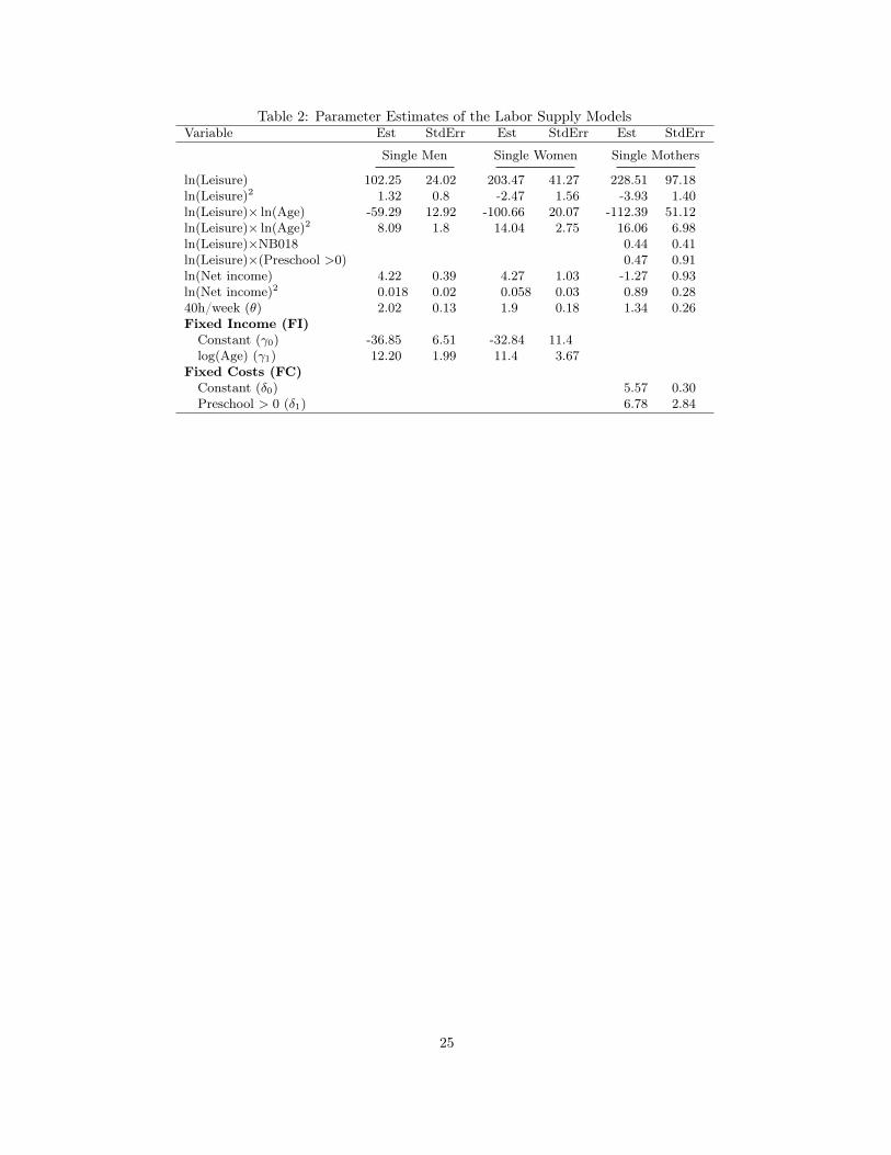
Table 2: Parameter Estimates of the Labor Supply ModelsVariable Est StdErr Est StdErr Est StdErr
Single Men Single Women Single Mothers
ln(Leisure) 102.25 24.02 203.47 41.27 228.51 97.18ln(Leisure)2 1.32 0.8 -2.47 1.56 -3.93 1.40ln(Leisure)× ln(Age) -59.29 12.92 -100.66 20.07 -112.39 51.12ln(Leisure)× ln(Age)2 8.09 1.8 14.04 2.75 16.06 6.98ln(Leisure)×NB018 0.44 0.41ln(Leisure)×(Preschool >0) 0.47 0.91ln(Net income) 4.22 0.39 4.27 1.03 -1.27 0.93ln(Net income)2 0.018 0.02 0.058 0.03 0.89 0.2840h/week (θ) 2.02 0.13 1.9 0.18 1.34 0.26Fixed Income (FI)Constant (γ0) -36.85 6.51 -32.84 11.4log(Age) (γ1) 12.20 1.99 11.4 3.67
Fixed Costs (FC)Constant (δ0) 5.57 0.30Preschool > 0 (δ1) 6.78 2.84
25
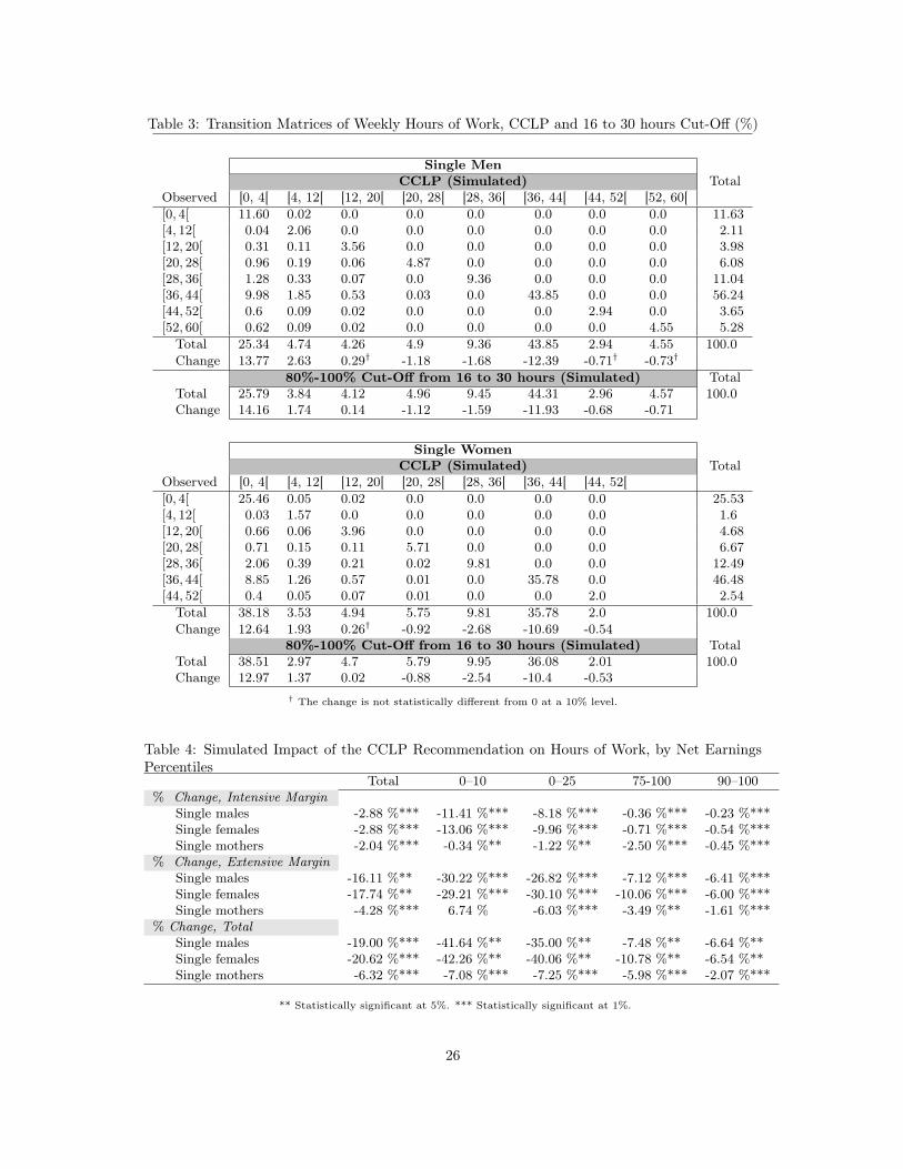
Table 3: Transition Matrices of Weekly Hours of Work, CCLP and 16 to 30 hours Cut-Off (%)
Single MenCCLP (Simulated) Total
Observed [0, 4[ [4, 12[ [12, 20[ [20, 28[ [28, 36[ [36, 44[ [44, 52[ [52, 60[[0, 4[ 11.60 0.02 0.0 0.0 0.0 0.0 0.0 0.0 11.63[4, 12[ 0.04 2.06 0.0 0.0 0.0 0.0 0.0 0.0 2.11[12, 20[ 0.31 0.11 3.56 0.0 0.0 0.0 0.0 0.0 3.98[20, 28[ 0.96 0.19 0.06 4.87 0.0 0.0 0.0 0.0 6.08[28, 36[ 1.28 0.33 0.07 0.0 9.36 0.0 0.0 0.0 11.04[36, 44[ 9.98 1.85 0.53 0.03 0.0 43.85 0.0 0.0 56.24[44, 52[ 0.6 0.09 0.02 0.0 0.0 0.0 2.94 0.0 3.65[52, 60[ 0.62 0.09 0.02 0.0 0.0 0.0 0.0 4.55 5.28Total 25.34 4.74 4.26 4.9 9.36 43.85 2.94 4.55 100.0Change 13.77 2.63 0.29† -1.18 -1.68 -12.39 -0.71† -0.73†
80%-100% Cut-Off from 16 to 30 hours (Simulated) TotalTotal 25.79 3.84 4.12 4.96 9.45 44.31 2.96 4.57 100.0Change 14.16 1.74 0.14 -1.12 -1.59 -11.93 -0.68 -0.71
Single WomenCCLP (Simulated) Total
Observed [0, 4[ [4, 12[ [12, 20[ [20, 28[ [28, 36[ [36, 44[ [44, 52[[0, 4[ 25.46 0.05 0.02 0.0 0.0 0.0 0.0 25.53[4, 12[ 0.03 1.57 0.0 0.0 0.0 0.0 0.0 1.6[12, 20[ 0.66 0.06 3.96 0.0 0.0 0.0 0.0 4.68[20, 28[ 0.71 0.15 0.11 5.71 0.0 0.0 0.0 6.67[28, 36[ 2.06 0.39 0.21 0.02 9.81 0.0 0.0 12.49[36, 44[ 8.85 1.26 0.57 0.01 0.0 35.78 0.0 46.48[44, 52[ 0.4 0.05 0.07 0.01 0.0 0.0 2.0 2.54Total 38.18 3.53 4.94 5.75 9.81 35.78 2.0 100.0Change 12.64 1.93 0.26† -0.92 -2.68 -10.69 -0.54
80%-100% Cut-Off from 16 to 30 hours (Simulated) TotalTotal 38.51 2.97 4.7 5.79 9.95 36.08 2.01 100.0Change 12.97 1.37 0.02 -0.88 -2.54 -10.4 -0.53
† The change is not statistically different from 0 at a 10% level.
Table 4: Simulated Impact of the CCLP Recommendation on Hours of Work, by Net EarningsPercentiles
Total 0–10 0–25 75-100 90–100% Change, Intensive Margin
Single males -2.88 %*** -11.41 %*** -8.18 %*** -0.36 %*** -0.23 %***Single females -2.88 %*** -13.06 %*** -9.96 %*** -0.71 %*** -0.54 %***Single mothers -2.04 %*** -0.34 %** -1.22 %** -2.50 %*** -0.45 %***
% Change, Extensive MarginSingle males -16.11 %** -30.22 %*** -26.82 %*** -7.12 %*** -6.41 %***Single females -17.74 %** -29.21 %*** -30.10 %*** -10.06 %*** -6.00 %***Single mothers -4.28 %*** 6.74 % -6.03 %*** -3.49 %** -1.61 %***
% Change, TotalSingle males -19.00 %*** -41.64 %** -35.00 %** -7.48 %** -6.64 %**Single females -20.62 %*** -42.26 %** -40.06 %** -10.78 %** -6.54 %**Single mothers -6.32 %*** -7.08 %*** -7.25 %*** -5.98 %*** -2.07 %***
** Statistically significant at 5%. *** Statistically significant at 1%.
26
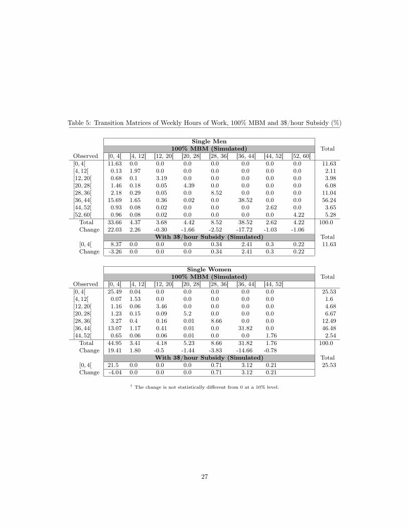
Table 5: Transition Matrices of Weekly Hours of Work, 100% MBM and 3$/hour Subsidy (%)
Single Men100% MBM (Simulated) Total
Observed [0, 4[ [4, 12[ [12, 20[ [20, 28[ [28, 36[ [36, 44[ [44, 52[ [52, 60[[0, 4[ 11.63 0.0 0.0 0.0 0.0 0.0 0.0 0.0 11.63[4, 12[ 0.13 1.97 0.0 0.0 0.0 0.0 0.0 0.0 2.11[12, 20[ 0.68 0.1 3.19 0.0 0.0 0.0 0.0 0.0 3.98[20, 28[ 1.46 0.18 0.05 4.39 0.0 0.0 0.0 0.0 6.08[28, 36[ 2.18 0.29 0.05 0.0 8.52 0.0 0.0 0.0 11.04[36, 44[ 15.69 1.65 0.36 0.02 0.0 38.52 0.0 0.0 56.24[44, 52[ 0.93 0.08 0.02 0.0 0.0 0.0 2.62 0.0 3.65[52, 60[ 0.96 0.08 0.02 0.0 0.0 0.0 0.0 4.22 5.28Total 33.66 4.37 3.68 4.42 8.52 38.52 2.62 4.22 100.0Change 22.03 2.26 -0.30 -1.66 -2.52 -17.72 -1.03 -1.06
With 3$/hour Subsidy (Simulated) Total[0, 4[ 8.37 0.0 0.0 0.0 0.34 2.41 0.3 0.22 11.63Change -3.26 0.0 0.0 0.0 0.34 2.41 0.3 0.22
Single Women100% MBM (Simulated) Total
Observed [0, 4[ [4, 12[ [12, 20[ [20, 28[ [28, 36[ [36, 44[ [44, 52[[0, 4[ 25.49 0.04 0.0 0.0 0.0 0.0 0.0 25.53[4, 12[ 0.07 1.53 0.0 0.0 0.0 0.0 0.0 1.6[12, 20[ 1.16 0.06 3.46 0.0 0.0 0.0 0.0 4.68[20, 28[ 1.23 0.15 0.09 5.2 0.0 0.0 0.0 6.67[28, 36[ 3.27 0.4 0.16 0.01 8.66 0.0 0.0 12.49[36, 44[ 13.07 1.17 0.41 0.01 0.0 31.82 0.0 46.48[44, 52[ 0.65 0.06 0.06 0.01 0.0 0.0 1.76 2.54Total 44.95 3.41 4.18 5.23 8.66 31.82 1.76 100.0Change 19.41 1.80 -0.5 -1.44 -3.83 -14.66 -0.78
With 3$/hour Subsidy (Simulated) Total[0, 4[ 21.5 0.0 0.0 0.0 0.71 3.12 0.21 25.53Change -4.04 0.0 0.0 0.0 0.71 3.12 0.21
† The change is not statistically different from 0 at a 10% level.
27
Tab
le6:
Estim
ated
Costof
theCCLP
Recom
menda
tion
,Withan
dW
itho
utLa
borSu
pply
Adjustm
ents
(Tho
usan
ds2004
$)Item
Sing
lemen
Sing
leWom
enSing
leMothe
rsTotal
Per
Cap
ita
No
Beh
avio
ural
Adju
stmen
ts
Que
becgovernmentCost
229769
178108
51826
459703
611
Cost
per
capi
ta595
671
515
611
Wit
hB
ehav
ioural
Adju
stmen
ts
Fede
ralIncom
eTax
es-172,600***
-87,020***
-13,166***
-272,786***
-363***
ProvincialIncom
eTax
es-189,100***
-90,189***
-14,475***
-293,764***
-391***
Fede
ralT
ransfers
-891***
-2,712***
798***
-2,805***
-4***
ProvincialT
ransfers
6,700***
1,918***
1,021***
9,639***
13***
Social
Assistance
207,600***
111,700***
20,857***
340,157***
452***
QPP
-85,812***
-45,610***
-6,190***
-137,612***
-183***
EmploymentInsurance
-38,083***
-20,572***
-2,670***
-61,325***
-82***
CCLP
590,900***
393,100***
62,007***
1,046,007***
1,391***
Cost:
Province
1,080,052***
642,473***
104,550***
1,827,075***
2,429***
per
capi
ta2,798***
2,420***
1,039***
Cost:
Provincial+
Fede
ral
1,289,829***
747,352***
121,184***
2,158,365***
2,870***
per
capi
ta3,342***
2,815***
1,204***
Num
berof
individu
als
385,962
265,469
100,669
752,100
***Statisticallysign
ificant
at1%.
28

Table 7: Cost of Alternative Policy Simulations (Thousands $)Single Single Single TotalMen Women Mothers Total
CCLP recommendationSubsidy 590,900 393,100 62,007 1,046,007Provincial Cost 1,080,052 642,473 104,550 1,827,074Total Cost 1,289,829 747,352 121,184 2,158,366Income increase (%) 11.9 14.0 5.3 11.8Income decrease (%) 17.0 15.4 5.6 14.9No change (%) 71.1 70.6 89.1 73.3
CCLP with threshold at 30 HoursSubsidy 566,400 381,300 56,504 1,004,204Provincial Cost 1,046,560 626,863 97,050 1,770,473Total Cost 1,249,056 728,334 112,384 2,089,774Income increase (%) 11.9 13.9 5.3 11.8Income decrease (%) 16.4 15.0 5.4 14.4No change (%) 71.7 71.1 89.4 73.9
100% of the MBMSubsidy 1,112,000 708,500 132,100 1,952,600Provincial Cost 1,881,864 1,100,327 222,618 3,204,810Total Cost 2,198,815 1,257,780 253,925 3,710,520Income increase (%) 12.2 15.5 13.7 13.5Income decrease (%) 24.1 20.8 8.2 20.8No change (%) 63.7 63.9 78.1 65.7
3$ Wage subsidy for Non-WorkersSubsidy 169,000 136,500 56,380 361,880Provincial Cost 99,911 72,473 28,928 201,312Total Cost 54,848 31,636 18,647 105,132Income increase (%) 3.3 4.0 4.0 3.6Income decrease (%) 0 0 0 0No change (%) 96.7 96.0 96.0 96.4
29
[0, 4[ [4, 12[ [12, 20[ [20, 28[ [28, 36[ [36, 44[ [44, 52[ [52, 60[
ObservedPredicted
Predicted/Observed Hours of Work Single Men
Weekly hours of work
Per
cent
age
010
2030
4050
60
(a) Single Men
[0, 4[ [4, 12[ [12, 20[ [20, 28[ [28, 36[ [36, 44[ [44, 52[
ObservedPredicted
Predicted/Observed Hours of Work Single Women
Weekly hours of work
Per
cent
age
010
2030
4050
60
(b) Single Women
[0, 5[ [5, 15[ [15, 25[ [25, 35[ [35, 45[ [45, 55[
ObservedPredicted
Predicted/Observed Hours of Work Single Mothers
Weekly hours of work
Per
cent
age
010
2030
4050
60
(c) Single Mothers
Figure 4: Model Fit for Different Samples
30
A Econometric Model
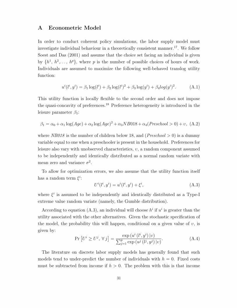
In order to conduct coherent policy simulations, the labor supply model mustinvestigate individual behaviour in a theoretically consistent manner.17. We followSoest and Das (2001) and assume that the choice set facing an individual is givenby {h1, h2,. . . , hp}, where p is the number of possible choices of hours of work.Individuals are assumed to maximize the following well-behaved translog utilityfunction:
ui(li, yi) = β1 log(li) + β2 log(l
i)2 + β3 log(yi) + β4log(y
i)2. (A.1)
This utility function is locally flexible to the second order and does not imposethe quasi-concavity of preferences.18 Preference heterogeneity is introduced in theleisure parameter β1:
β1 = α0 +α1 log(Age)+α2 log(Age)2 +α3NB018+α4(Preschool > 0)+ υ, (A.2)
where NB018 is the number of children below 18, and (Preschool > 0) is a dummyvariable equal to one when a preschooler is present in the household. Preferences forleisure also vary with unobserved characteristics, υ, a random component assumedto be independently and identically distributed as a normal random variate withmean zero and variance σ2.
To allow for optimization errors, we also assume that the utility function itselfhas a random term ξi:
U i(li, yi) = ui(li, yi) + ξi, (A.3)
where ξi is assumed to be independently and identically distributed as a Type-Iextreme value random variate (namely, the Gumble distribution).
According to equation (A.3), an individual will choose hi if ui is greater than theutility associated with the other alternatives. Given the stochastic specification ofthe model, the probability this will happen, conditional on a given value of υ, isgiven by:
Pr[U i ≥ U j, ∀ j
]=
exp (ui (li, yi) |υ)∑pj=1 exp (u
j (lj, yj) |υ). (A.4)
The literature on discrete labor supply models has generally found that suchmodels tend to under-predict the number of individuals with h = 0. Fixed costsmust be subtracted from income if h > 0. The problem with this is that income
31
minus fixed costs may be negative, a possibility that cannot be dealt with dueto the form of the translog utility function. Gong and van Soest (2002) haveintroduced the notion of fixed income for not working. Instead of subtracting afixed cost to work, a fixed income can be added to the income at zero hours ofwork, making inactivity a relatively more attractive alternative. Both approacheshave the potential to capture the bunching at zero hours of work. For practicalreasons, the model for single mothers is based upon the “fixed costs” approach,while the models for single males and females are based upon the “fixed income”approach.19
Fixed incomes and fixed costs are incorporated into the model by replacingu (yi, li) by u (y0 + FI, l0) and u (yi − FC, li) ,∀i > 0, respectively. The precisespecification is
FI = γ0 + γ1 ln (A) (A.5)
FC = δ0 + δ1(Preschool > 0). (A.6)
Equation (A.5) assumes that the fixed income is related to age and equation(A.6) states that the fixed costs of working are associated with the presence ofpreschoolers. The two specifications could be made to depend on a richer set ofcovariates. To save on the degrees of freedom, the most parsimonious specificationthat nevertheless fitted the data well was selected.
We make one last modification to the standard model to account for the bunchingof weekly hours of work around 40. We thus write:
U i(li, yi) = ui(li, yi) + θ(h = 40), (A.7)
where (h = 40) is a dummy indicator equal to one if the individual works exactly40 hours per week. The parameter θ proxies a fixed effect that increases the utilityassociated with working forty hours per week.
Finally, note that equation (A.4) is written conditionally on a given realization ofthe random component υ. The unconditional probability is obtained by integratingit out:
Pr[U i ≥ U j, ∀ j
]=
∫exp (ui (li, yi) |υ)∑pj=1 exp (u
j (lj, yj) |υ)φ(υ; 0, σ2
)dυ, (A.8)
where φ is the density of υ. Because υ is assumed to follow a normal distribution,
32
equation (A.8) does not have a closed-form solution. We thus simulate the inte-gration by drawing R = 100 draws of υq, q = 1, ..., R, from the normal distributionfor each observation and compute the expected probability (3.3) as:
P̂r[ui ≥ uj ∀ j
]=
1
R
R∑q=1
exp (ui (li, yi) |υq)∑pj=1 exp (u
j (lj, yj) |υq). (A.9)
The maximization of the simulated likelihood function yields consistent and effi-cient parameter estimates if
√N/R→ 0 when R→ +∞ and N → +∞ (N being
the number of observations; see Gouriéroux and Monfort 1991; 1996).20
The parameter estimates on fixed income reported in Table 2 tell an interestingstory. The parameter associated with log(Age) is positive for both single males andfemales and is highly statistically significant. Older singles thus behave as thoughthey have stronger preferences for leisure. Likewise, the parameter associated with(h = 40) is also positive and highly statistically significant. In our framework, thisis equivalent to depicting a strong preference for working the standard workweek.
The parameters of the fixed costs term are also intuitively consistent. The pa-rameter estimates show that the fixed costs to work increase when preschoolers arepresent in the household. They thus make working a less attractive alternative.Single mothers, like single males and females, also behave as though they have astrong preference for the standard workweek.
33