1

Filipe Marques, António P. Souto, Paulo Flores, On the constraints violation in forward dynamics of multibody systems. Multibody System Dynamics, 39(4), 385–419 (2017)

On the constraints violation in forward dynamics of multibody systems

Filipe Marques1, António P. Souto2 and Paulo Flores1,∗

1 Department of Mechanical Engineering, University of Minho Campus de Azurém, 4804-533 Guimarães, Portugal

2 Department of Textile Engineering, University of Minho

Campus de Azurém, 4804-533 Guimarães, Portugal

Abstract It is known that the dynamic equations of motion for constrained mechanical multibody systems are frequently formulated using the Newton-Euler’s approach, which is augmented with the acceleration constraint equations. This formulation results in the establishment of a mixed set of partial differential and algebraic equations, which are solved in order to predict the dynamic behavior of general multibody systems. The classical resolution of the equations of motion is highly prone to constraints violation because the position and velocity constraint equations are not fulfilled. In this work, a general and comprehensive methodology to eliminate the constraints violation at the position and velocity levels is offered. The basic idea of the described approach is to add corrective terms to the position and velocity vectors with the intent to satisfy the corresponding kinematic constraint equations. These corrective terms are evaluated as function of the Moore-Penrose generalized inverse of the Jacobian matrix and of the kinematic constraint equations. The described methodology is embedded in the standard method to solve the equations of motion based on the technique of Lagrange multipliers. Finally, the effectiveness of the described methodology is demonstrated through the dynamic modeling and simulation of different planar and spatial multibody systems. The outcomes in terms of constraints violation at the position and velocity levels, conservation of the total energy and computational efficiency are analyzed and compared with those obtained with the standard Lagrange multipliers method, the Baumgarte stabilization method, the augmented Lagrangian formulation, the index-1 augmented Lagrangian and the coordinate partitioning method. Keywords: Constraints violation, Baumgarte stabilization method, Penalty method, Augmented Lagrangian formulation, Index-1 Lagrangian formulation, Coordinate partitioning method, Mechanical energy, Computational efficiency, Forward dynamics, Multibody systems

∗ Corresponding author, Tel: + 351 253510220, Fax: +351 253516007, E-mail: pflores@dem.uminho.pt

2

1. Introduction Multibody dynamics deals with the study of the motion characteristics of many bodies whose

interactions are modeled by forces and constraints. The problem of modeling and simulating

constrained multibody systems has been widely studied over the last decades [1-9]. Recent

review papers of interest on the formulation of multibody systems have been provided by

Rahnejat [10], Udwadia [11] Eberhard and Schiehlen [12], Schiehlen [13] and Nikravesh [14].

The various formulations of dynamics of constrained multibody systems differ in the principle

considered, type of coordinates adopted and the method selected for handling constraints in

systems characterized by open and closed-loop topologies [15-22]. The solution of dynamic

equations of motion for constrained multibody systems is often performed by using Lagrange

multipliers technique, which leads to a set of differential and algebraic equations. Except for

simple mechanical systems, the analytical solution of the equations of motion cannot be found,

but in the most common cases require numerical resolution. In the standard Lagrange multipliers

technique, the acceleration constraint equations are taken into account during the numerical

resolution of the equations of motion and, therefore, there is no violation of the acceleration

constraints. In sharp contrast, the position and velocity constraint equations are not utilized and,

consequently, violation of the constraints at the position and velocity levels will occur due to the

numerical integration errors. Thus, special procedures have to be implemented to eliminate or at

least minimize the violation of the constraints [7, 23-30].

In a broad sense, the methods to handle the problem of constraints violation for dynamics

of constrained multibody systems fall into three main categories: (i) constraint stabilization

approaches; (ii) coordinate partitioning methods and (iii) direct correct formulations [23]. The

constraint stabilization approaches are probably the most popular due to their simplicity and

easiness for computational implementation. However, their major drawback is the ambiguity in

selecting the stabilization parameters, which ultimately can lead to failure simulations, even for

systems that have valid solutions [31]. In turn, the coordinate partitioning methods have the great

merit of allowing the rigorous resolution of the constraint equations at the position, velocity and

acceleration levels. However, they can suffer from poor numerical efficiency when it is

necessary to change the independent coordinate set [32]. The direct formulations, which include

the projection methods, have physical meaning, computational efficiency, but they can exhibit

some numerical instability [33]. There is no doubt that the constraint stabilization approaches

and the direct correct formulations are the most popular and utilized methods to deal with the

problem of constraints violation [7, 27-29, 34-44].

3

The Baumgarte stabilization method is the most widely utilized technique to overcome

the limitations of the standard resolution of the dynamic equations of motion, which is borrowed

from the feedback control theory [45]. The principle of this method is based on the addition of

two terms to the acceleration constraint equations in order to stabilize the violations in the

position and velocity constraint equations. This method has been extended to the problem of

violation stabilization of holonomic systems formulated by using the canonical momenta

approach [46]. The original Baumgarte method is very straightforward and easy to incorporate in

any general multibody computational code [21]. In fact, this approach has been utilized

successfully for many applications [47-59]. One of the problems associated with the Baumgarte

stabilization method deals with the ambiguity in choosing feedback parameters, which

eventually can seriously influence the dynamic equations of motion and get poor simulation

results. In fact, as pointed out by Baumgarte [45], the selection of the stabilization parameters

usually involves a trial and error procedure. The problem of selection of the stabilization

parameters has been object of many research works over the last few decades. Ascher et al. [60]

explained the difficulties of the parameter choice for Baumgarte stabilization and introduced

improved constraint stabilization techniques. Chang and Nikravesh [61] presented an adaptive

methodology for determining the optimum values of the stabilization parameters associated with

the Baumgarte method. The effectiveness of this methodology was demonstrated through its

application to two examples that illustrate the improvements in reducing the constraints

violation. Bae and Yang [62] and Yoon and coworkers [63] developed different techniques to

select the Baumgarte stabilization parameters. Lin and Hong [64] highlighted that the use to

positive values for Baumgarte stabilization parameters is not sufficient to ensure convergence of

the constraint equations at position and velocity levels. Lin and Huang [65] presented a method

to select the stabilization parameters where the Runge-Kutta algorithm was employed. This work

used the stability analysis method in digital control theory. More recently, Flores and his co-

workers [31] presented a parametric study on the Baumgarte stabilization method. In this work

the authors analyzed and discussed the influence of the stabilization parameters, integration

method, time step and quality of the initial conditions on the dynamic response of planar

constrained multibody systems.

Park and Chiou [66] developed a constraint stabilization approach similar to the

Baumgarte method by using a penalty form of the constraint equations, which integrates two

different sets of equations, one for the coordinates and another one for the Lagrange multipliers

[67]. Ostermeyer [68], based on optimum control theory, improved the Baumgarte method. Yoon

et al. [69] presented an effective method to deal with the energy constraint control in numerical

4

simulation of constrained mechanical systems. The method is developed based on the geometric

interpretation of the relation between constraints in the phase space. Several combinations of

energy constraint control with either Baumgarte’s constraint violation stabilization method or the

new constraint violation stabilization using gradient feedback are also addressed. A new method

for implementing constraint controls is developed by using the Euler method for integrating

constraint control terms. Inspired on the seminal work of Baumgarte, Hong et al. [70] proposed

an implicit constraint enforcement approach that is stable over large time steps and does not

require problem dependent stabilization parameters. This technique utilizes the future time step

to estimate the correct magnitude of the constraint forces, resulting in better stability over higher

time steps. In addition, this formulation is physically conforming and minimizes the constraint

drifts. In later work, Hong et al. [71] presented an implicit holonomic and non-holonomic

constraint enforcement method for rigid body dynamics that ensures numerical stability without

requiring ad-hoc stabilization parameters. This technique provides the same asymptotic

computational cost as the Baumgarte method. Weijia and co-authors [72], also based on the

Baumgarte method, presented an automatic formulation for the constraints violation stabilization

of the numerical solution of the equations of motion in the context of dynamics of multibody

systems. They use the Taylor expansion series to determine a relation between the stabilization

parameters and the integration time step. Cline and Pai [73] proposed a post-stabilization

approach for rigid multibody systems simulation. This approach compensates the error of

integration each time step to correct the constraint error. However, the post-stabilization requires

a linear system solution to find the error correction and it does not preserve the correct dynamic

motion of objects when it reduces constraint drifts. Alternative techniques to deal with the

problem of the constraint violation stabilization have been proposed by many researchers [74-

78]. A detailed and complete review on the main approaches for constraint enforcement in the

context of multibody dynamics has been performed by Bauchau and Laulusa [29] and Vlasenko

and Kasper [41].

In the coordinate partitioning method, the generalized coordinates are partitioned into

independent and dependent sets [79], being the numerical integration carried out for independent

generalized coordinates. Then, the constraint equations are solved for dependent generalized

coordinates. The advantage of this method is that it satisfies all the constraints to the level of

precision specified and maintains good error control. However, it can suffer from poor numerical

efficiency when it is necessary to change the independent coordinate set. Nikravesh and Haug

[80] proposed a comprehensive method based on the generalized coordinate partitioning for

analysis of multibody systems with holonomic and non-holonomic constraints. In this work, a

5

Gaussian elimination scheme with full pivoting is utilized to decompose the constraint Jacobian

matrix and identifies independent coordinates. Haug and Yen [81] also investigated on the

coordinate partitioning approach for numerical integration of differential-algebraic equations

under the framework of multibody dynamics. The accuracy of this formulation has been

demonstrated, both from theoretical and numerical points of view. Fisette and Vaneghem [33],

based on the coordinate partitioning method, used the LU factorization of constraints Jacobian

matrix to identify the dependent and independent coordinates. This aspect is of paramount

importance since during the integration process, numerical problems may arise due to inadequate

choice of the independent coordinates that lead to poorly conditioned matrices. This problem

was also considered by Arabyan and Wu [82] to study multibody mechanical systems with both

holonomic and non-holonomic constraints. Neto and Ambrósio [32] also utilized the coordinate

partitioning method to handle the constraints violation correction for the integration of

differential algebraic equations in the presence of redundant constraints. It must be highlighted

that the coordinate partitioning methods are effective and very useful [83-85] and a good number

of investigations haven been carried out on the establishment of the sets of independent and

dependent coordinates. In fact, over the last few decades, several approaches that allows for the

selection of the independent set of coordinates have been proposed [86-91]. Recently, Carpinelli

et al. [92] studied the problem of the accuracy and efficiency of the implicit Euler approach

when switching from dependent to independent coordinates. For this, an automatic procedure is

implemented.

In the direct correct formulations, the violation of constraint equations are eliminated

during the numerical resolution of the DAE equations of motion [29]. Over the last years, several

techniques have been developed to eliminate the constraints violation, namely those by Bayo et

al. [74] Lubich [93], Andrzejewski and Bock [94], Yu and Chen [95] and Blajer [27]. Eich [96]

presented a coordinate projection method that allows for the control of the constraints violation

in mechanical multibody systems with algebraic constraints. Yoon et al. [97] presented a direct

correction formulation to eliminate the violation of the constraints in numerical simulation of

constrained multibody systems. This method corrects the values of the state variables directly so

that they can fit the constraint equations well. However, this method is formulated at the

positions level only. Blajer [98] considered the projection method to obtain the dynamic

equations of motion for constrained multibody systems in the form of ordinary differential

equations. Then, a standard solver was used to integrate the resulting system. In a later work

Blajer [99] presented a unified geometric formulation for constrained multibody systems. Blajer

highlighted that the negligence of the inertial properties of the systems can result in physical

6

inconsistency. A method that allows for the elimination of the constraints violation has been

proposed by Aghili and Piedboeuf [100], which is based on the concept of pseudo-inverse of the

constraint matrix. This formulation is able to solve the problem associated with redundant

constraints and singularities in mechanical multibody systems. Tseng et al. [101] used the

Maggi’s equations with perturbed iteration to develop an efficient approach to numerically solve

the dynamic equations of motion of constrained multibody systems. This approach, named

integrate-and-collaborate paradigm, has the goal to execute coupled system simulation without

sacrificing the integrity of subsystem modeling and solutions, and to maintain the effectiveness

of the overall results. Nikravesh [102] proposed a direct method to obtain appropriate the initial

coordinates and velocities, where the basic idea is to correct the values of the state variables

before the numerical solution of the dynamic equations of motion take place. Recently, Zhang et

al. [103] presented a physically consistent methodology to suppress the violation of the

constraint equations of three-dimensional multibody systems, in which the mass matrix is

singular. For this purpose, the constrained and weighted least-squares-based geometrical

projection method is considered in the resolution of the equations of motion, and the explicit

correction formulation is formulated by the block matrix inversion procedure. The effectiveness

of this methodology is demonstrated trough several benchmark examples of application, where

the constraints at the position level are precisely ensured with a few number of iterations, while

the constraints at the velocity level are guaranteed with a single step procedure.

Alternative methodologies to handle the elimination of the constraints violation have

been addressed by other researchers, being the interested reader referred to the following

references [35, 75, 76, 83, 84, 104-106]. For instance, Cuadrado and his coworkers [35]

presented a comparative analysis for four methodologies to handle constrained multibody

systems, namely the augmented Lagrangian formulation with projections in index-1 and index-3,

a modified state-space formulation based on the projection matrices and a fully-recursive

formulation. Four different benchmark problems have been considered to effectively assess the

influence of the approach utilized in terms of computational efficiency, accuracy and

performance. Terze et al. [76, 83, 84] proposed an integration method for dynamic simulation of

constrained multibody systems with no constraint violation. In a first stage, the set of

independent variables are identified and selected, and then the displacement constraint violations

were eliminated in an iterative process. In a second stage, considering the constraints equations

at the velocity level eliminated the velocity constraint violations. In turn, Yu and Chen [95]

presented a direct violation correction approach both at the position and velocity levels. The

effectiveness of the approach was validated and compared with standard formulation and

7

Baumgarte method applied to a simple planar four bar mechanism. Bayo and Ledesma [104]

combined the well-established augmented Lagrangian formulation together with a mass

orthogonal projection technique for constrained multibody systems. This particular approach has

been successfully employed by many researchers, due to its computational robustness, accuracy

and efficiency. In fact, the utilization of the mass orthogonal projection technique is quite

effective and minimizes the constraints violation at the machine accuracy level. Orden and

coauthors [105, 106] investigated on the energy balance of a velocity projection providing an

alternative interpretation of its effect on the stability and a practical criterion for the mass-

orthogonal projection matrix selection. More recently, Terze and coworkers [107, 108] has

investigated on the Lie-group integration method for constrained multibody systems in state

space. The proposed approach avoids the kinematical differential equations because the

formulation integration algorithm is developed on the system manifold via MBS element’s

angular velocities and rotational matrices. This is of paramount importance since they can

eliminate the problems associated with singularities. With the purpose of eliminating the

numerical constraint violations at both the positions and velocity levels during the integration

scheme, a projection method based on constrained least-square minimization algorithm was

presented. The easiness and effectiveness of the proposed approach was demonstrated

throughout the simulation of two numerical examples of application, namely the heavy top

dynamics and the satellite with mounted 5-DOF manipulator. The approach seems to be especial

useful for discrete mechanical systems that incorporate general kinematical constraints and for

systems that describes large 3D rotations [107].

The main emphasis of this work is on the elimination of the constraints violation during

the dynamic analysis of constrained multibody systems. Body coordinates formulation is used to

describe the system components and the kinematic joints. The equations governing the dynamic

behavior of the general mechanical systems incorporate corrective terms that are added to the

position and velocity vectors in order to satisfy the corresponding constraint equations. These

corrective terms are expressed in terms of the Jacobian matrix and kinematic constraint

equations. Moreover, the corrective terms are added and considered during the numerical

resolution of the dynamic equations of motion. In the sequel of this process, the standard method

based on the Lagrange multipliers technique, the Baumgarte stabilization method, the

coordinating partitioning method, the penalty approach and the augmented Lagrangian

formulation have been revisited. Results for several planar and spatial multibody mechanical

systems are presented and utilized to discuss the assumptions and procedures adopted throughout

this work.

8

2. Equations of motion for constrained multibody systems

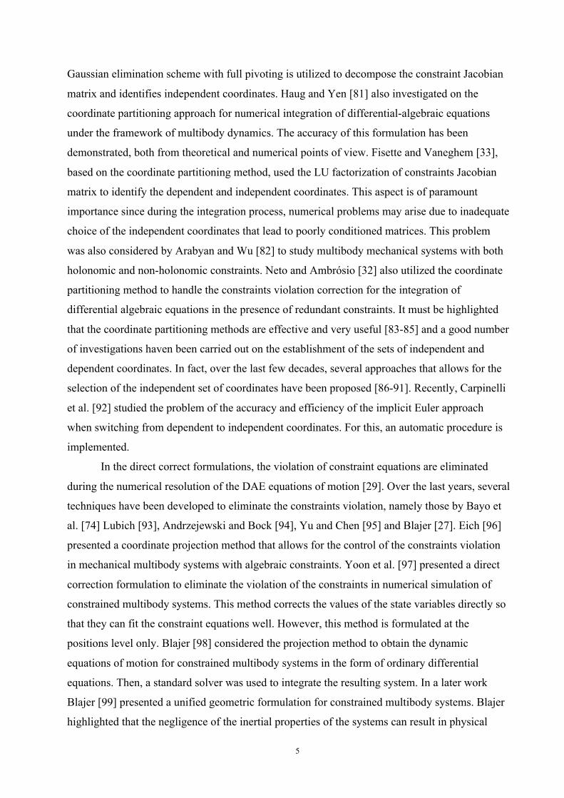
In a simple manner, a mechanical multibody system embraces two main features, namely (i)

mechanical components that describe large translational and rotational motions and (ii)

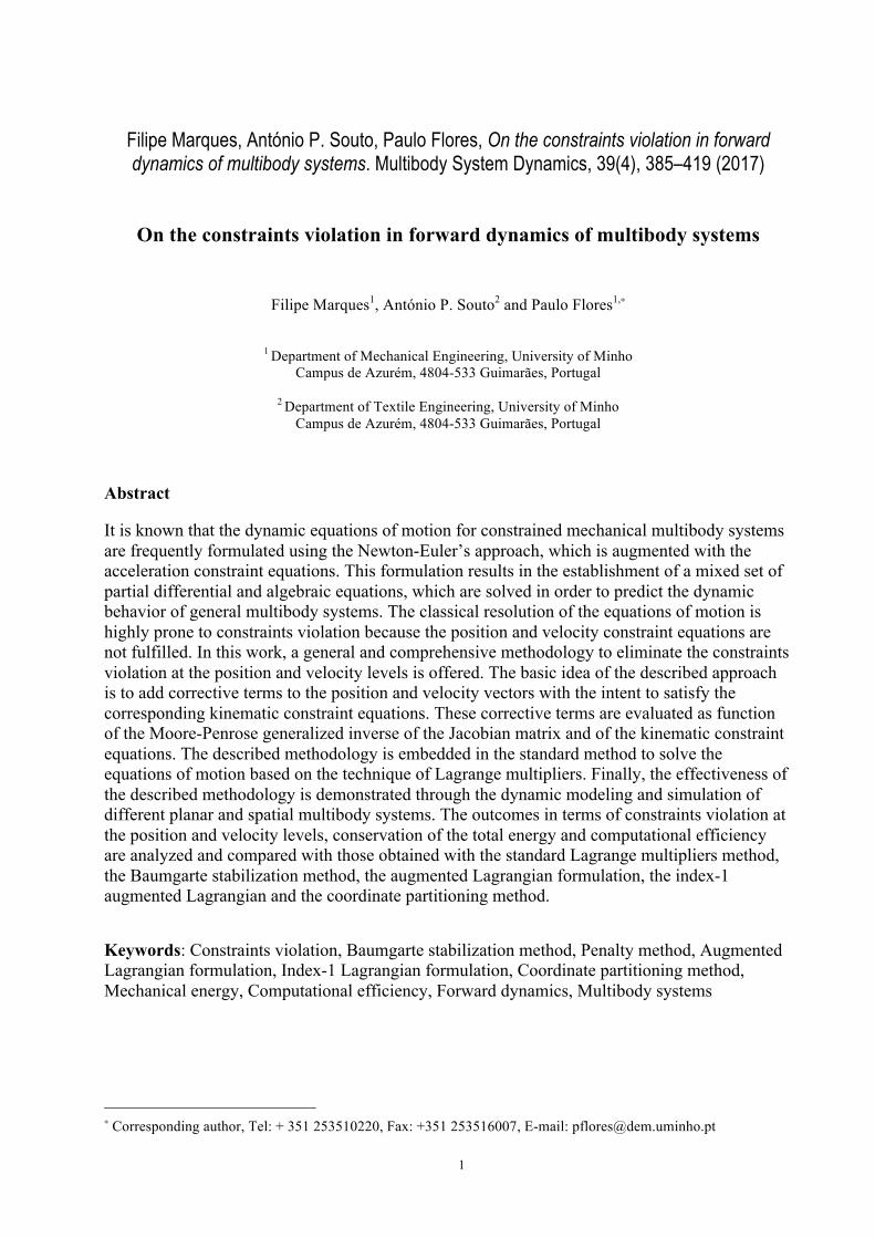
kinematic joints that impose some constraints on the relative motion of the bodies [2-4]. Figure 1

depicts a generic configuration of a spatial multibody system that encompasses a collection of

rigid and flexible bodies interconnected by kinematic joints and acted upon by force elements.

The forces applied over the multibody system components can be the result of springs, dampers,

actuators or external forces. External applied forces of different nature and different levels of

complexity can act on a multibody system with the purpose to simulate the interaction among the

system components and between these and the surrounding environment [109, 110].

Body 1

Gravitational forces

Body n

Body 3

Body i

Body 2

Spring

Spherical joint

Applied torque

Actuator

Flexible body

Spherical joint with clearance

Revolute joint

Fig. 1 Generic representation of a mechanical multibody system with its most significant

components: bodies, joints and forces elements.

In order to be able to analyze the dynamic response of constrained mechanical multibody

systems, it is first necessary to formulate the equations of motion that govern the behavior of

multibody systems. For this purpose, let the configuration of a constrained mechanical multibody

system be described by n generalized coordinates, then a set of m algebraic kinematic

independent scleronomic constraints Φ can be written in a compact form as [2]

( )≡ =Φ Φ q 0 (1)

where q is the vector of generalized coordinates. The number of generalized coordinates, n, and

the number of kinematic constraints, m, must be adequately selected, bearing in mind the correct

system’s description and system’s degrees of freedom [21]. In the most general case, the

9

constraint equation (1) encompasses the total set of holonomic and non-holonomic restrictions to

which a generic multibody system can be subjected [11]. The velocities and accelerations of the

system components are evaluated by using the velocity and acceleration constraint equations.

Thus, the first time derivative of Eq. (1) provides the velocity constraint equations as

Φ ≡ Dv = 0 (2)

where D denotes the system Jacobian matrix and v is the vector of generalized velocities.

A second differentiation of Eq. (1) with respect to time leads to acceleration constraint

equations as

Φ ≡ Dv + Dv = 0 (3)

in which v is the generalized accelerations and the term − Dv is referred to as the right-hand

side of the acceleration equations. By introducing γ = − Dv , Eq. (3) can be rewritten as

Dv = γ (4)

For a multibody system of constrained bodies, the Newton-Euler equations of motion are

written as [2, 4]

Mv = g + g(c) (5)

where M is the global mass matrix, g is the vector of generalized forces and g(c) denotes the

vector of reaction forces that can be expressed in terms of the constraints Jacobian matrix and

Lagrange multipliers, λ , as

( )c T=g D λ (6)

Finally, the translational and rotational equations of motion for a constrained multibody

system can be expressed in its general form as

Mv −DTλ = g (7)

In dynamic analysis, a unique solution is obtained when the algebraic constraint

equations at the acceleration level are considered simultaneously with the differential equations

of motion together with a set of appropriate initial conditions [4]. Therefore, Eq. (4) is appended

to Eq. (7), yielding a system of differential and algebraic equations written as

M −DT

D 0

⎡

⎣⎢⎢

⎤

⎦⎥⎥vλ

⎧⎨⎪

⎩⎪

⎫⎬⎪

⎭⎪=

gγ

⎧⎨⎪

⎩⎪

⎫⎬⎪

⎭⎪ (8)

This linear system of equations can be solved by applying any method suitable for the

resolution of linear algebraic equations. The existence of null elements in the main diagonal of

10

the leading matrix and the possibility of ill-conditioned matrices suggest that methods using

partial or full pivoting are preferred. The dynamic equations of motion can also be solved

analytically. For this purpose, Eq. (7) is rearranged to put the accelerations vector in evidence,

yielding

v =M−1(g +DTλ) (9)

In this process, it is assumed that the inverse of the mass matrix M exists. It must be

emphasized that a unique solution of Eq. (8) is guaranteed when the mass matrix is positive

definite and the Jacobian matrix has a maximum rank [4]. This particular issue has been

analyzed in detail in the seminal work by Jalón and Gutiérrez-López [90]. Introducing Eq. (9)

into Eq. (4) and after basic mathematical manipulation results in

λ = DM−1DT⎡⎣ ⎤⎦−1(γ −DM−1g) (10)

Substituting now Eq. (10) into Eq. (9) yields

v =M−1g +M−1DT DM−1DT⎡⎣ ⎤⎦−1(γ −DM−1g){ } (11)

Thus, Eq. (11) is solved for v then, the velocities and positions can be obtained by

numerical integration. This procedure must be repeated until the final time of analysis is reached.

This manner to solve the dynamic equations of motion is commonly referred to as the standard

Lagrange multipliers method [2].

At this stage, it must be highlighted that some numerical difficulties can arise when

solving the dynamic equations of motion. As already stated, in general, it is assumed that the

mass matrix is always invertible. However, it has been demonstrated in many research studies

that the mass matrix can be singular, namely when more than six coordinates are considered to

define the pose of a rigid body [39, 41, 90, 111, 112]. Another problem can appear when a body

in the system under analysis has extremely small inertia [39, 90, 111]. A third problem that often

can take place is associated with redundant constraints. Additional difficulties that can occur in

the resolution of the equations of motion are related to systems with changing topologies [22]

and units [113]. Within the spirit of the present study, these issues are not object of investigation,

being the interested reader referred to the following references [4, 22, 23, 32, 42, 43, 76, 90, 101,

105, 111-118].

11

The system of the equations of motion (8) or (11) does not use explicitly the position and

velocity equations associated with the kinematic constraints, that is, Eqs. (1) and (2). In other

words, after the numerical resolution of the Eq. (8), both constraints at the position and velocity

levels are not satisfied. Consequently, for moderate or long simulations, the original constraint

equations start to be violated due to the integration process and/or to inaccurate initial conditions.

Therefore, methods able to eliminate errors in the position and velocity equations or, at least, to

keep such errors under control, must be adopted. In order to keep the constraint violations under

control, the Baumgarte stabilization method is considered here [45]. This method allows

constraints to be slightly violated before corrective actions can take place, in order to force the

violation to vanish. The objective of Baumgarte method is to replace the differential equation (3)

by the following expression

Φ + 2α Φ + β 2Φ = 0 (12)

Equation (12) is a differential equation for a closed-loop system in terms of kinematic

constraint equations, in which the terms 2α Φ and 2β Φ play the role of control terms. The

principle of the method is based on the damping of acceleration of constraints violation by

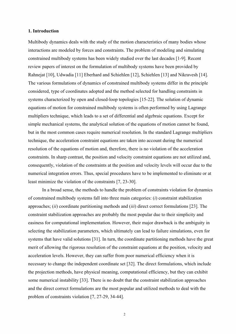
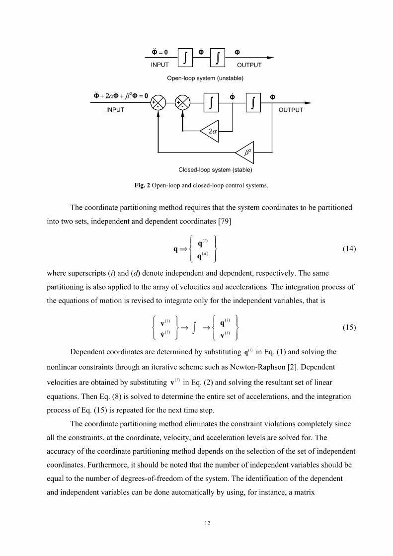
feeding back the position and velocity of constraints violation. Figure 2 illustrates open and

closed-loop control systems. It is known that in the open-loop systems Φ and Φ do not

converge to zero if any perturbation occurs and, therefore, the system is unstable. Thus, using the

Baumgarte approach, the equations of motion for a system subjected to kinematic constraints can

be stated in the following form

M −DT

D 0

⎡

⎣⎢⎢

⎤

⎦⎥⎥vλ

⎧⎨⎪

⎩⎪

⎫⎬⎪

⎭⎪=

gγ − 2α Φ −β2Φ

⎧⎨⎪

⎩⎪

⎫⎬⎪

⎭⎪ (13)

If the gain parameters, α and β, are chosen as positive constants, in general systems, the

stability of the general solution of Eq. (13) is guaranteed. Baumgarte [45] highlighted that the

suitable choice of the parameters α and β can be performed by numerical experiments. Hence,

the Baumgarte method has some ambiguity in determining optimal feedback gains. The improper

choice of these parameters can lead to unacceptable results in the dynamic analysis of the

multibody systems. Over the last decades, a good number of works have been published on the

selection of the gain parameters and their influence on the systems’ response [31, 47, 51, 53, 55-

58, 60, 63, 70, 71, 119].

12

=Φ 0

INPUT OUTPUT

Φ∫

Φ∫

Open-loop system (unstable)

Closed-loop system (stable)

INPUT OUTPUT

22α β+ + =Φ Φ Φ 0 Φ Φ∫ ∫

2β

2α

+ -- +

Fig. 2 Open-loop and closed-loop control systems.

The coordinate partitioning method requires that the system coordinates to be partitioned

into two sets, independent and dependent coordinates [79]

q⇒q(i )

q(d )⎧⎨⎪

⎩⎪

⎫⎬⎪

⎭⎪ (14)

where superscripts (i) and (d) denote independent and dependent, respectively. The same

partitioning is also applied to the array of velocities and accelerations. The integration process of

the equations of motion is revised to integrate only for the independent variables, that is

v(i )

v(i )⎧⎨⎪

⎩⎪

⎫⎬⎪

⎭⎪→ ∫ → q(i )

v(i )⎧⎨⎪

⎩⎪

⎫⎬⎪

⎭⎪ (15)

Dependent coordinates are determined by substituting q( i) in Eq. (1) and solving the

nonlinear constraints through an iterative scheme such as Newton-Raphson [2]. Dependent

velocities are obtained by substituting v(i ) in Eq. (2) and solving the resultant set of linear

equations. Then Eq. (8) is solved to determine the entire set of accelerations, and the integration

process of Eq. (15) is repeated for the next time step.

The coordinate partitioning method eliminates the constraint violations completely since

all the constraints, at the coordinate, velocity, and acceleration levels are solved for. The

accuracy of the coordinate partitioning method depends on the selection of the set of independent

coordinates. Furthermore, it should be noted that the number of independent variables should be

equal to the number of degrees-of-freedom of the system. The identification of the dependent

and independent variables can be done automatically by using, for instance, a matrix

13

factorization technique, such as Gaussian elimination with full pivoting [32]. One drawback of

this method is that the choice of the independent variables may change during a simulation,

mostly due to large rotations of bodies. Although switching from one set of independent variable

to another during a simulation is possible, the associated computational overhead can be costly.

Furthermore, the computational effort associated with the Newton-Raphson process can, in some

cases, be considered as another drawback. A good number of researchers have been utilized the

coordinate partitioning method in the field of multibody dynamics [23, 32, 33, 79-82, 86, 87,

120-122]. It has been stated by some authors that the coordinate partitioning method is not very

efficient from numerical point of view due to the necessity to solve the nonlinear constraint

equations and also due to the need to change the independent coordinates. However, the

coordinate partitioning method can be very interesting and efficient when combined with the

Maggi’s formulation, as it has been shown in the literature [28, 101, 123, 124].

The penalty method presented by Jalón and Bayo [7] constitutes an alternative way to

solve the dynamic equations of motion. In this method, the equations of motion are modeled as a

linear second-order differential equation that can be written in the form

mc Φ + dc Φ + kcΦ = 0 (16)

Introducing Eq. (3) into Eq. (16) yields

mc (Dv + Dv) + dc Φ + kcΦ = 0 (17)

Pre-multiplying Eq. (17) by the transpose of Jacobian matrix, DT, and after mathematical

treatment, results in

mcDTDv = −DT (mc Dv + dc Φ + kcΦ) (18)

Let consider now the Newton-Euler equations of motion for a system of unconstrained

system and written here as [2]

Mv = g (19)

Adding Eqs. (18) and (19) yields

Mv + mcDT Dv = g − DT (−mcγ + dc

Φ + kcΦ) (20)

in which Eq. (4) has been employed. Finally, Eq. (20) can be rewritten in the following form

(M +αDTD) v = g −αDT (−γ + 2µω Φ +ω 2Φ) (21)

where

α = mc , 2c cd mµω= and 2c ck mω= (22)

14

Equation (21) can be solved for v . This penalty method gives good results if α tends to

infinity. Typical values of α, ω and µ are 1×107, 10 and 1, respectively [7, 125]. It should be

noted that with this penalty method, multibody systems with redundant constraints or kinematic

singular configurations can be solved. In fact, the penalty method has been utilized to evaluate

the constraint forces in multibody systems with redundant constraints [111, 117, 118]. However,

this approach cannot handle the problem of solving indetermination of the Lagrange multipliers,

as it was analyzed by Jalón and Gutiérrez-López [90].

The augmented Lagrangian formulation, which can be seen as an evolution of the penalty

method, is a methodology that penalizes the constraints violation, much in the same form as the

Baumgarte stabilization method. This is an iterative procedure that presents advantages relative

to other methods because it involves the solution of a smaller set of equations, handles redundant

constraints and still delivers accurate results in the vicinity of singular configurations [7, 104].

Let index i denote the i-th iteration. Thus, based on the work by Bayo and Ledesma [104], the

evaluation of the system accelerations in a given time step starts as

Mvi = g , (i=0) (23)

The iterative process to evaluate the system accelerations proceeds with the evaluation of

(M +αDTD) vi+1 =Mvi −αDT (−γ + 2µω Φ +ω 2Φ) (24)

This iterative process continues until

v i+1 − v i = ε (25)

where ε is a specified tolerance [104].

The augmented Lagrangian method involves the solution of a system of equations with a

dimension equal to the number of coordinates of the multibody system. Though mass matrix M

is generally positive semi-definite the leading matrix of Eq. (24) Tα+M D D is always positive

definite [7, 29]. Bayo and coworkers [126] extended and simplified the original augmented

Lagrangian formulation and demonstrated that the penalty terms associated with the velocity

constraints are needed to avoid the high frequency oscillations that can appear during the

numerical resolution of the equations of motion. It has been shown by many researchers that the

implementation of the augmented Lagrangian formulation is quite effective, efficient and robust

when performing forward dynamic simulations. Finally, it must be stated that the selection of the

penalty factors must avoid the numerical ill problems associated with flexibility of bodies,

compliance of kinematic joints and manufacturing and assemble errors [90, 101, 104, 127].

15

Alternative formulations based on projections onto the constraints manifolds to fulfill the

constraint equations have been proposed over the last decades, such as those by Bayo and

Ledesma [104]. In particular, the index-1 augmented Lagrangian method with mass-orthogonal

projections, which is based on the augmented Lagrangian formulation, utilizes the projections of

positions and velocities to completely satisfy the constraints equations. In contrast to the other

approaches, the index-1 augmented Lagrangian method is not applied during the resolution of

the dynamic equations of motion. Thus, the generalized positions and velocities of the system, q0

and v0, respectively, are calculated using any integration scheme, which does not ensure the

fulfillment of the constraints equations at position and velocity levels.

A mass-orthogonal projection of the solution is performed in order to obtain a corrected

set of positions, which enforces the application of the following iterative procedure according to

1 0( ) ( )T Ti i iα ++ = − − −M D D Δq M q q D λ (26)

with

1 1i i i+ += +q q Δq (27)

1 1i i iα+ += +λ λ Φ (28)

Similarly to Eq. (25), this iterative procedure involving Eqs. (26)-(28) is applied until the

following condition is verified

1i ε+ =Δq (29)

It is clear that when the initial approximation q0 is close to the corrected set of

coordinates, the modified Newton-Raphson method can be employed to improve the efficiency

of this method.

A similar mass-orthogonal projection is performed at the velocity level. The inaccurate

set of velocities obtained from numeric integration, v0, is updated solving the following system

[104]

1( )T Ti iα α++ = −M D D v Mv D υ (for rheonomic constraints) (30a)

1( )Ti iα ++ =M D D v Mv (for scleronomic constraints ) (30b)

It can be observed that the leading matrix Tα+M D D depends only on the generalized

positions of the system, therefore, it does not need to be updated in each iteration. The interested

reader in formulations based on projections onto constraints manifolds is referred to the recent

work by Cuadrado et al. [128], Dopico et al. [129.] and González et al. [130, 131].

16

3. Direct correction approach to eliminate the constraints violation

The main purpose of this section is to present a general and comprehensive direct correction

approach to deal with the elimination of the constraints violation at both position and velocity

levels. For this, let consider that during the numerical resolution of the dynamic equations of

motion, the vector of generalized coordinates needs to be corrected due to the constraints

violation. Thus, the corrected positions can be expressed in the form

δc u= +q q q (31)

where qu denotes the uncorrected positions and δq represents the set of corrections that

eliminates the constraints violation. This means that the corrective term has to be added to vector

qu in order to ensure that the constraint equations (1) are satisfied, that is

Φ(qc ) = Φ(qu ) + δΦ = 0 (32)

The term δΦ in Eq. (32) can be understood as the variation of the constraint equations

and can be expressed as [132]

δΦ = ∂Φ∂q1

δq1 +∂Φ∂q2

δq2 + ...+∂Φ∂qn

δqn = Dδq (33)

Combining now Eqs. (32) and (33) yields

Φ(qu ) +Dδq = 0 (34)

which ultimately leads to

δq = −D−1Φ(qu ) (35)

In general, the Jacobian matrix, D, is not square, therefore, D-1 does not exist. However,

the concept of the Moore-Penrose inverse matrix, D+, can be employed as [133-135]

1( )T T+ −=D D DD (36)

such that

+ =DD D D (37)

+ + +=D DD D (38)

and both D+D and DD+ are symmetric matrices. Consequently, it is possible to establish the

following mathematical relation [82],

1( ) ( ) ( )T T T T T− + + + + + + += = = =D DD D D D D D D D DD D (39)

Thus, Eq. (35) can be rewritten in the following form

δq = −DT (DDT )−1Φ(qu ) (40)

17

Finally, introducing Eq. (40) into Eq. (31) yields

qc = qu −DT (DDT )−1Φ(qu ) (41)

that represents the corrected generalized coordinates in each integration time step. It must be

noticed that the kinematic constraint equations at the position level are, in general, nonlinear,

then Eq. (41) must be solved iteratively by employing a numerical algorithm, such as the

Newton-Raphson method.

In a similar manner, the vector of generalized velocities can be corrected as

vc = vu + δv (42)

where δv is the term that has to be added to vector vu to guarantee that the velocity constraint

equations (2) are satisfied, that is

Φ(qc ,vc ) = Φ(qc ,vu ) + δ Φ = 0 (43)

The term δ Φ represents the variation of the velocity constraint equations expressed as

δ Φ = ∂ Φ∂q

δq + ∂ Φ∂ q

δ q (44)

The first term of the right-hand side of Eq. (44) is null because at this stage it is assumed

that the vector of generalized coordinates is already correct, and, consequently, δq=0. In turn, it

is known that the derivative of the velocity constraint equations with respect to vector of

generalized velocities is represented by the Jacobian matrix, D. Hence, Eq. (44) is simplified as

δ Φ = Dδv (45)

Now combining Eqs. (43) and (45) results in

Φ(qc ,vu ) +Dδv = 0 (46)

From Eq. (46) it is possible to obtain the term that corrects the vector of generalized

velocities as

δv = −D−1 Φ(qc ,vu ) (47)

Introducing now Eq. (36) into Eq. (47) results in

δv = −DT (DDT )−1 Φ(qc ,vu ) (48)

Finally, the substitution of Eq. (48) into Eq. (42) yields

vc = vu −DT (DDT )−1 Φ(qc ,vu ) (49)

that represents the corrected generalized velocities in each integration time step.

18

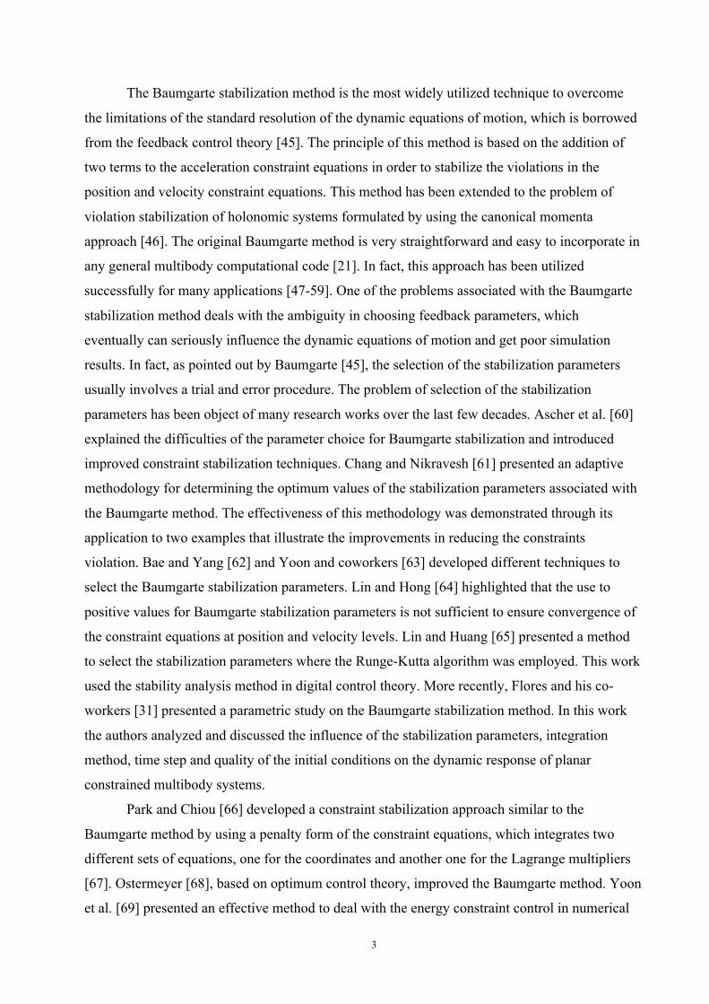
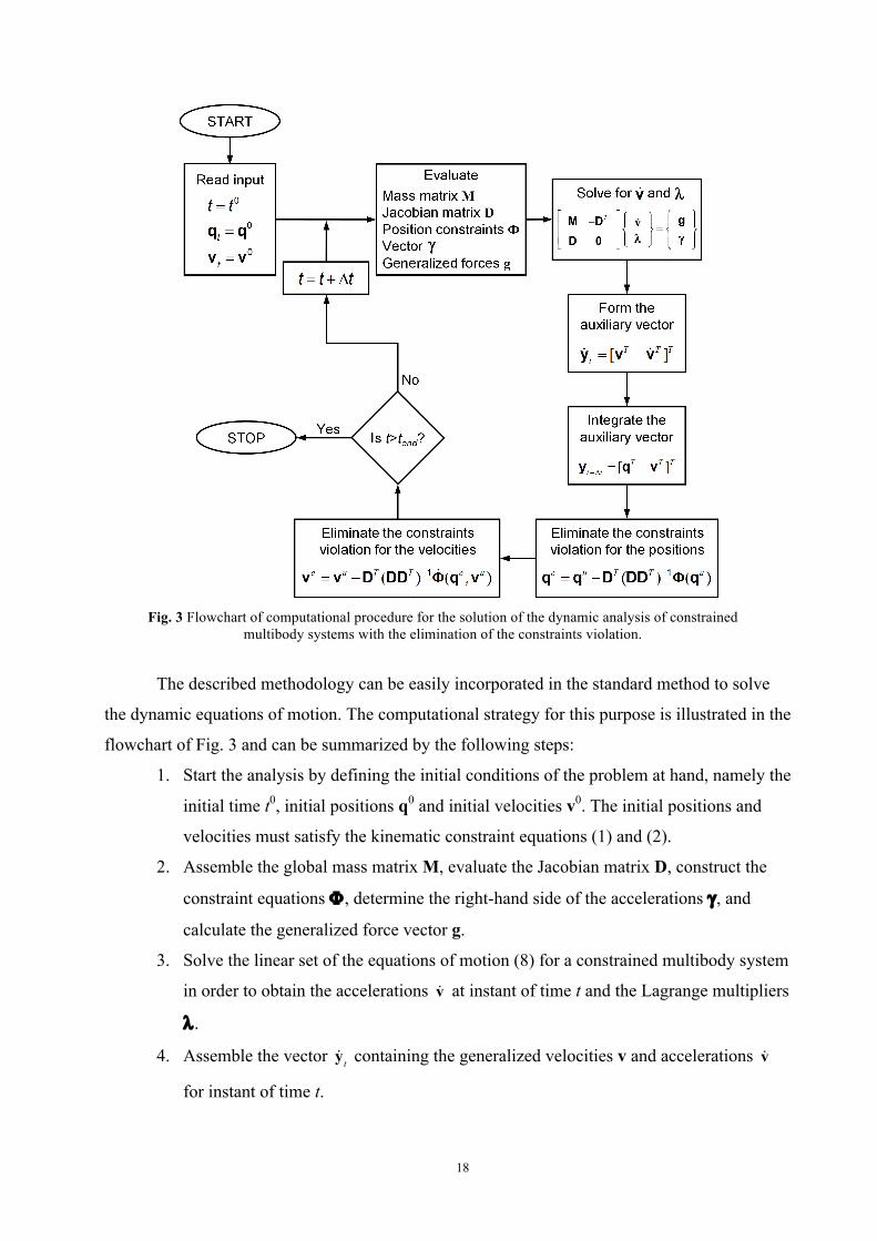
Fig. 3 Flowchart of computational procedure for the solution of the dynamic analysis of constrained

multibody systems with the elimination of the constraints violation.

The described methodology can be easily incorporated in the standard method to solve

the dynamic equations of motion. The computational strategy for this purpose is illustrated in the

flowchart of Fig. 3 and can be summarized by the following steps:

1. Start the analysis by defining the initial conditions of the problem at hand, namely the

initial time t0, initial positions q0 and initial velocities v0. The initial positions and

velocities must satisfy the kinematic constraint equations (1) and (2).

2. Assemble the global mass matrix M, evaluate the Jacobian matrix D, construct the

constraint equations Φ , determine the right-hand side of the accelerations γ , and

calculate the generalized force vector g.

3. Solve the linear set of the equations of motion (8) for a constrained multibody system

in order to obtain the accelerations v at instant of time t and the Lagrange multipliers

λ .

4. Assemble the vector yt containing the generalized velocities v and accelerations v

for instant of time t.

19

5. Integrate numerically the velocity and acceleration vectors to obtain the positions and

velocities at the instant of time t+Δt.

6. Evaluate the position constraint violations Φ(qu ) , compute the corrective term δq, by

using Eq. (40), and correct the positions vector employing Eq. (41). This step must be

repeated if necessary.

7. Evaluate the velocity constraint violations Φ(qc ,vu ) , compute the corrective term δv,

by using Eq. (48), and correct the velocities vector employing Eq. (49). It must be

stated that in this process the matrix D is evaluated with new values for qc.

8. Update the time variable, go to step 2) and proceed with the process for a new time

step, until the final time of analysis is reached.

In opposition to the constraint stabilization approaches, the methodology described above

is able to eliminate the violation of the constraints at both position and velocity levels without

changing the dynamic equations of motion. In fact, the proposed approach, by means of Eqs.

(41) and (49), refines the position and velocities computed solving the DAE system (8), being

the violation of constraints satisfied to machine accuracy.

The approach described above does not consider weighting factors to the coordinates and

velocities variables. In order to take into account different weighting factors, some works have

been proposed to include inertia of bodies, which allow for the adjustments to be made in an

inverse manner to the system inertia. The basic idea of this approach is that the more massive

bodies are moved the least if the constraints allow that [27, 98, 99, 102]. Thus, Eqs. (41) e (49)

are, respectively, substituted by

1( ) ( )c u T T u−= −q q MD DD Φ q (50)

vc = vu −MDT (DDT )−1 Φ(qc ,vu ) (51)

At this stage, it must be noticed that, in some circumstances, the evaluation of the

generalized inverse matrix given by Eq. (36) can exhibit numerical instabilities and can also be

cost from computational point of view. Thus, alternative methodologies can be adopted to

overcome these difficulties, namely using the approaches based on the singular value

decomposition (SVD) and the Gram-Schmidt Orthogonalization. The interested reader on

alternative methodologies is referred to the works by Neto and Ambrósio [32], Udwadia and

Phohomsiri [39], Mariti et al. [42], Arabyan and Wu [82], Jalón and Gutiérrez-López [90], Mani

and Haug [136], Singh and Likins [137], Kim and Vanderploeg [138], Meijaard [139].

20

4. Demonstrative examples of application A comparative study of several methods to handle the constraints violation is presented in this

section. For this purpose, different planar and spatial constrained mechanical systems are

considered in order to examine their effectiveness. The different methods are compared to each

other in terms of accuracy, conservation of energy and computational efficiency. The mechanical

multibody models analyzed, which include open and a closed-loop systems, are a planar four bar

mechanism, a spatial five pendulum system, a spatial slider-crank mechanism and a car

suspension. It must be stressed that for all the multibody models the initial conditions ensure the

position and velocity constraints [102]. All the methods have been implemented in a special-

purpose code, in which the fourth-order Runge-Kutta integrator scheme is utilized in the

numerical resolution of the dynamic equations of motion. All the multibody systems are

simulated and analyzed for a long time simulation period.

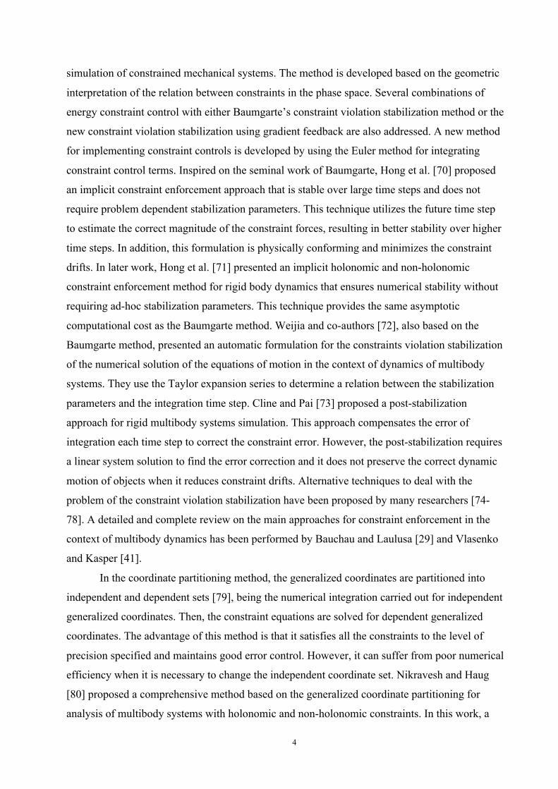
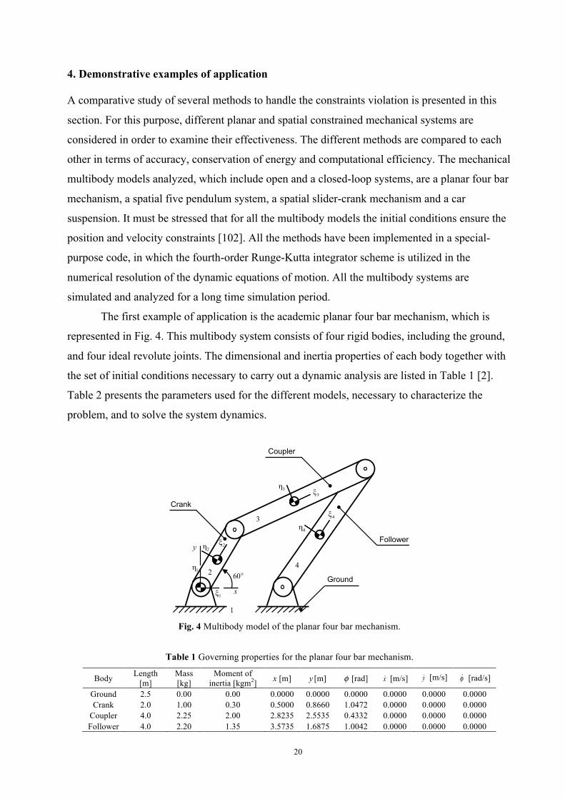
The first example of application is the academic planar four bar mechanism, which is

represented in Fig. 4. This multibody system consists of four rigid bodies, including the ground,

and four ideal revolute joints. The dimensional and inertia properties of each body together with

the set of initial conditions necessary to carry out a dynamic analysis are listed in Table 1 [2].

Table 2 presents the parameters used for the different models, necessary to characterize the

problem, and to solve the system dynamics.

1η

1ξ

3η3ξ

x

y

1

2

2η 2ξ

o60

3

4

4ξ

4η

Ground

Follower

Coupler

Crank

! Fig. 4 Multibody model of the planar four bar mechanism.

Table 1 Governing properties for the planar four bar mechanism.

Body Length [m]

Mass [kg]

Moment of inertia [kgm2] x [m] y [m] φ [rad] x [m/s] y [m/s]

φ [rad/s]

Ground 2.5 0.00 0.00 0.0000 0.0000 0.0000 0.0000 0.0000 0.0000 Crank 2.0 1.00 0.30 0.5000 0.8660 1.0472 0.0000 0.0000 0.0000

Coupler 4.0 2.25 2.00 2.8235 2.5535 0.4332 0.0000 0.0000 0.0000 Follower 4.0 2.20 1.35 3.5735 1.6875 1.0042 0.0000 0.0000 0.0000

21

Table 2 Parameters utilized for the dynamic simulations of the planar four bar mechanism.

Integration time step 1×10-3 s Penalty - α 1×107 Integrator algorithm Runge-Kutta - 4th order Penalty - ω 10 Baumgarte - α, β 5 Penalty - µ 1

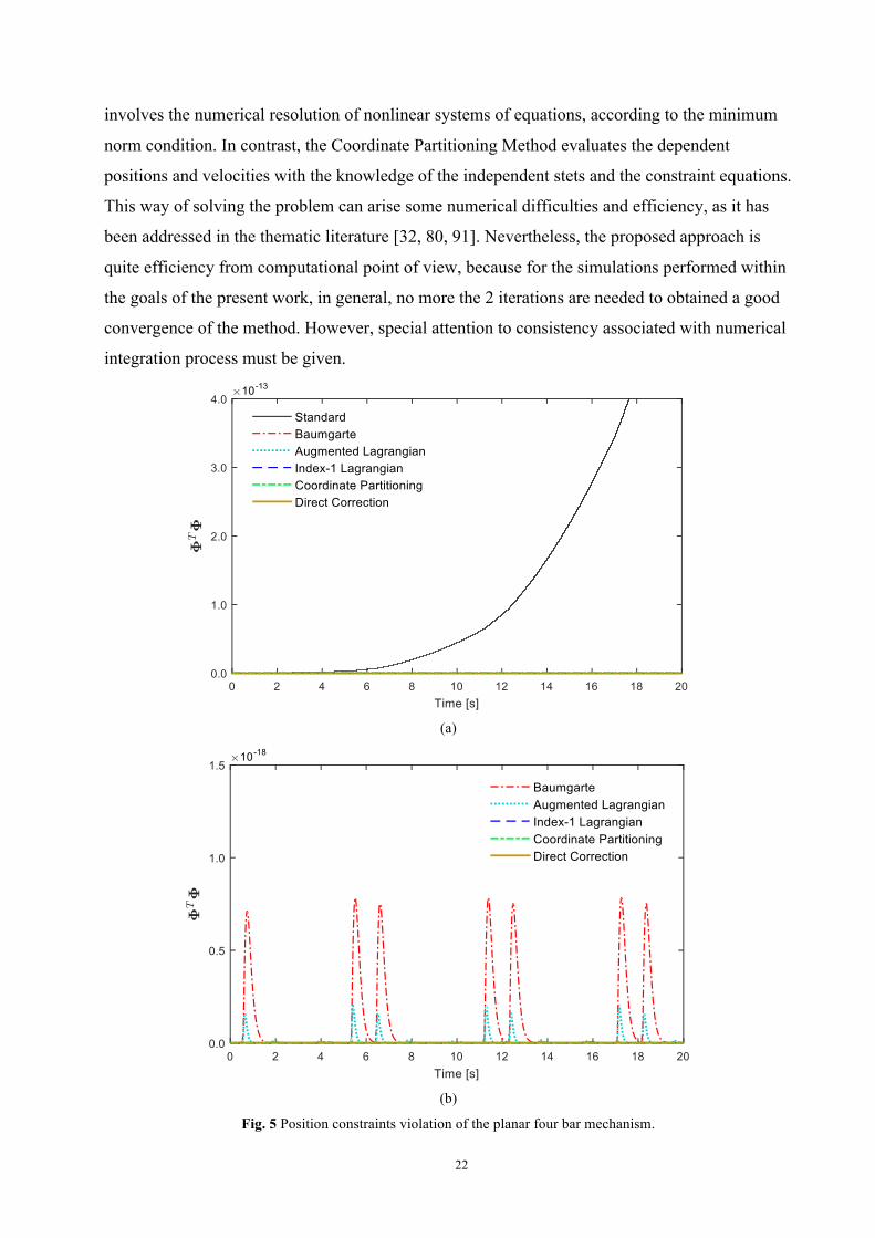
Figure 5 shows the plots of the constraints violation (ΦTΦ) resulting from the dynamic

simulation of the planar four bar mechanism. In this particular example, six methods are utilized

to solve the system dynamics, namely the standard Lagrange multipliers method, the Baumgarte

stabilization approach, the augmented Lagrangian formulation, the index-1 augmented

Lagrangian method, the coordinate partitioning method and the direct correction methodology

presented in the previous section. It should be highlighted that different scales are used for

results plotted in Figs. 5a and 5b, in order to clearly demonstrate the influence of the method

utilized. From the results shown in Fig. 5a, as expected, it can be observed that when the

standard Lagrange multipliers method is considered, the violation of constraints grows

indefinitely with the time [2, 23, 31]. However, when the Baumgarte stabilization method is

considered, the response is slightly different. In fact, with the Baumgarte approach, the

constraints violation does not growth with time, instead it tends to stabilize or stay under control,

as it can be observed from Fig. 5b. Furthermore, the augmented Lagrangian formulation exhibits

better behavior when compared to the previous analyzed approaches. Finally, it can be observed

that the index-1 augmented Lagrangian formulation, the coordinate partitioning method and the

direct correction approach completely eliminate the violation of constraints, visible the diagrams

of Fig. 5b. Indeed, with the methodology described in the previous section, the average of the

constraints violation is of order 1.0×10-18. It should be noticed that for the index-1 augmented

Lagrangian formulation, the coordinate partitioning method and the direct correction approach

the system performance in terms of constraints violation is coincident, and, consequently, the

corresponding lines are overlapped in bottom of the plots in Fig. 5. Finally, it must be stressed

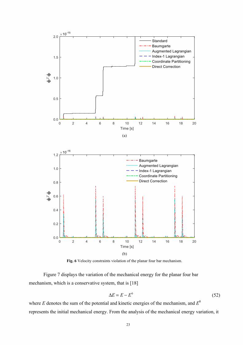
that a similar analysis and the same conclusions can be drawn from the diagrams plotted in Figs.

6a and 6b, corresponding to velocity constraints violation. Again, the different scales are utilized

for the results plotted in Figs. 6a and 6b, with the purpose to clearly observe the influence of the

methods used to resolve the system dynamics on the constraints violation. In general, the results

plotted for the dynamic simulation of the planar four bar mechanism are in line with those

published in [2, 7, 31, 32, 42, 70, 78, 127].

Finally, it must be stated that the proposed approach to deal with the constraints violation

changes all the coordinates to fulfill the constraint equations after the integration process, by

using Eqs. (40) and (41). This way of handle the constraints violation at the position level

22

involves the numerical resolution of nonlinear systems of equations, according to the minimum

norm condition. In contrast, the Coordinate Partitioning Method evaluates the dependent

positions and velocities with the knowledge of the independent stets and the constraint equations.

This way of solving the problem can arise some numerical difficulties and efficiency, as it has

been addressed in the thematic literature [32, 80, 91]. Nevertheless, the proposed approach is

quite efficiency from computational point of view, because for the simulations performed within

the goals of the present work, in general, no more the 2 iterations are needed to obtained a good

convergence of the method. However, special attention to consistency associated with numerical

integration process must be given.

(a)

(b)

Fig. 5 Position constraints violation of the planar four bar mechanism.

23

(a)

(b)

Fig. 6 Velocity constraints violation of the planar four bar mechanism.

Figure 7 displays the variation of the mechanical energy for the planar four bar

mechanism, which is a conservative system, that is [18]

ΔE = E − E0 (52) where E denotes the sum of the potential and kinetic energies of the mechanism, and E0

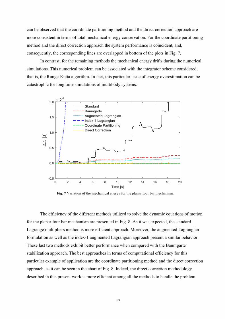
represents the initial mechanical energy. From the analysis of the mechanical energy variation, it

24

can be observed that the coordinate partitioning method and the direct correction approach are

more consistent in terms of total mechanical energy conservation. For the coordinate partitioning

method and the direct correction approach the system performance is coincident, and,

consequently, the corresponding lines are overlapped in bottom of the plots in Fig. 7.

In contrast, for the remaining methods the mechanical energy drifts during the numerical

simulations. This numerical problem can be associated with the integrator scheme considered,

that is, the Runge-Kutta algorithm. In fact, this particular issue of energy overestimation can be

catastrophic for long time simulations of multibody systems.

Fig. 7 Variation of the mechanical energy for the planar four bar mechanism.

The efficiency of the different methods utilized to solve the dynamic equations of motion

for the planar four bar mechanism are presented in Fig. 8. As it was expected, the standard

Lagrange multipliers method is more efficient approach. Moreover, the augmented Lagrangian

formulation as well as the index-1 augmented Lagrangian approach present a similar behavior.

These last two methods exhibit better performance when compared with the Baumgarte

stabilization approach. The best approaches in terms of computational efficiency for this

particular example of application are the coordinate partitioning method and the direct correction

approach, as it can be seen in the chart of Fig. 8. Indeed, the direct correction methodology

described in this present work is more efficient among all the methods to handle the problem

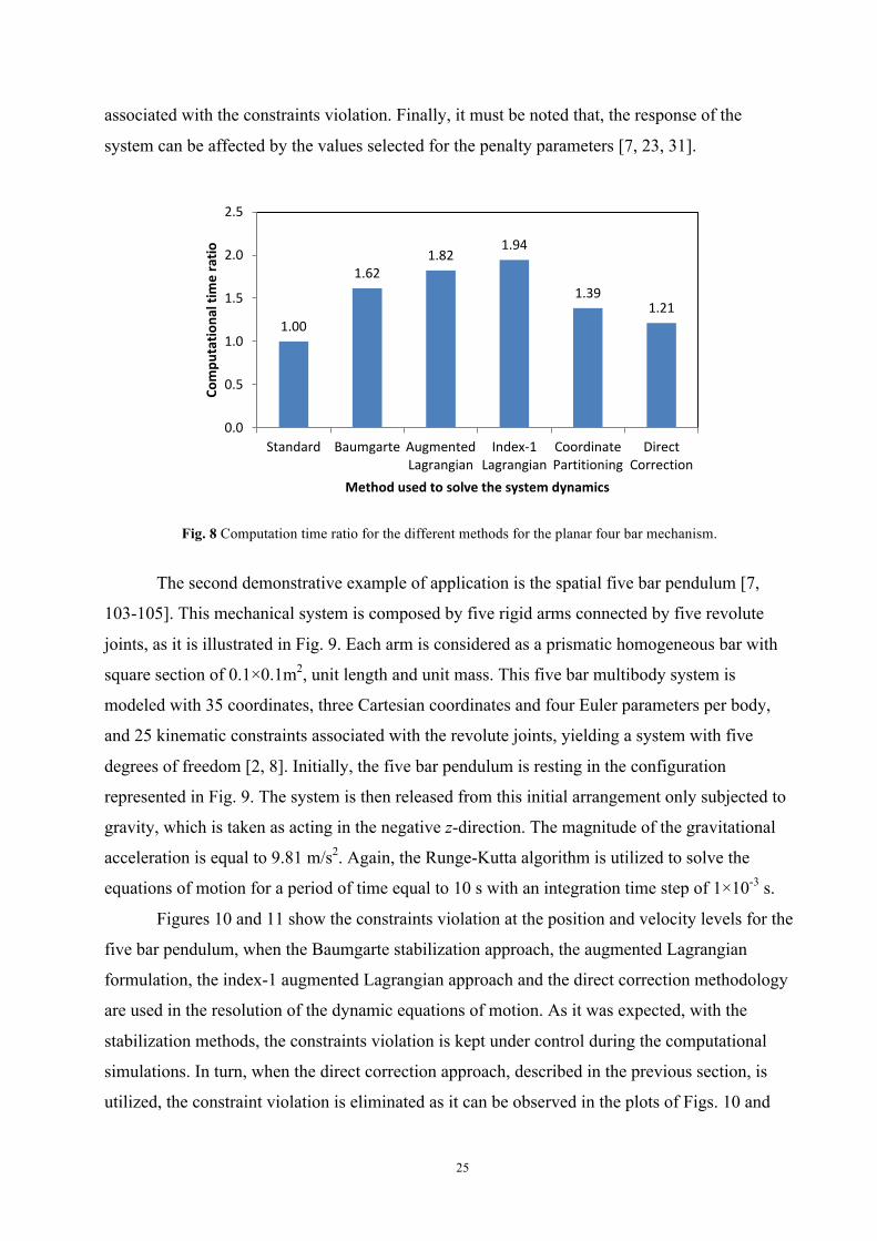
25

associated with the constraints violation. Finally, it must be noted that, the response of the

system can be affected by the values selected for the penalty parameters [7, 23, 31].

1.00

1.621.82

1.94

1.391.21

0.0

0.5

1.0

1.5

2.0

2.5

Standard Baumgarte AugmentedLagrangian

Index-­‐1Lagrangian

CoordinatePartitioning

DirectCorrection

Compu

tatio

nal  tim

e  ratio

Method  used  to  solve  the  system  dynamics

Fig. 8 Computation time ratio for the different methods for the planar four bar mechanism.

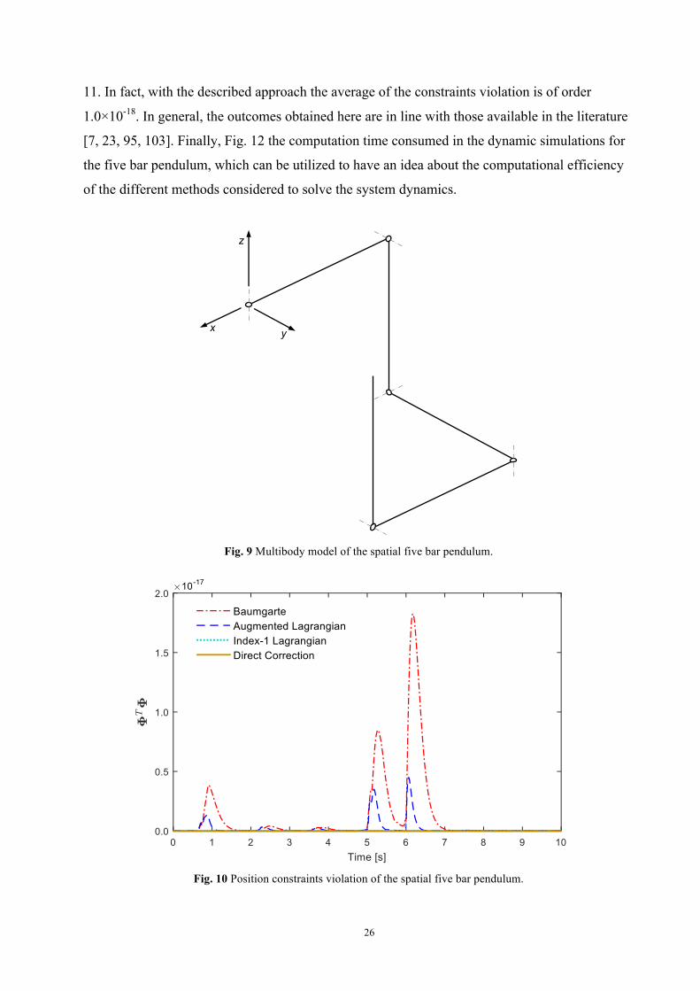
The second demonstrative example of application is the spatial five bar pendulum [7,

103-105]. This mechanical system is composed by five rigid arms connected by five revolute

joints, as it is illustrated in Fig. 9. Each arm is considered as a prismatic homogeneous bar with

square section of 0.1×0.1m2, unit length and unit mass. This five bar multibody system is

modeled with 35 coordinates, three Cartesian coordinates and four Euler parameters per body,

and 25 kinematic constraints associated with the revolute joints, yielding a system with five

degrees of freedom [2, 8]. Initially, the five bar pendulum is resting in the configuration

represented in Fig. 9. The system is then released from this initial arrangement only subjected to

gravity, which is taken as acting in the negative z-direction. The magnitude of the gravitational

acceleration is equal to 9.81 m/s2. Again, the Runge-Kutta algorithm is utilized to solve the

equations of motion for a period of time equal to 10 s with an integration time step of 1×10-3 s.

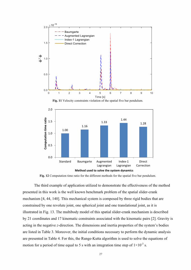
Figures 10 and 11 show the constraints violation at the position and velocity levels for the

five bar pendulum, when the Baumgarte stabilization approach, the augmented Lagrangian

formulation, the index-1 augmented Lagrangian approach and the direct correction methodology

are used in the resolution of the dynamic equations of motion. As it was expected, with the

stabilization methods, the constraints violation is kept under control during the computational

simulations. In turn, when the direct correction approach, described in the previous section, is

utilized, the constraint violation is eliminated as it can be observed in the plots of Figs. 10 and

26

11. In fact, with the described approach the average of the constraints violation is of order

1.0×10-18. In general, the outcomes obtained here are in line with those available in the literature

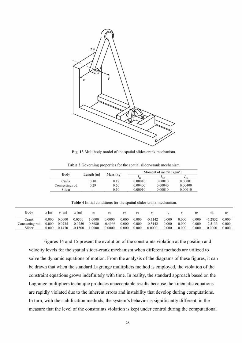
[7, 23, 95, 103]. Finally, Fig. 12 the computation time consumed in the dynamic simulations for

the five bar pendulum, which can be utilized to have an idea about the computational efficiency

of the different methods considered to solve the system dynamics.

x

z

y

Fig. 9 Multibody model of the spatial five bar pendulum.

Fig. 10 Position constraints violation of the spatial five bar pendulum.

27

Fig. 11 Velocity constraints violation of the spatial five bar pendulum.

1.001.16

1.331.44

1.28

0.0

0.5

1.0

1.5

2.0

Standard Baumgarte AugmentedLagrangian

Index-­‐1Lagrangian

DirectCorrection

Compu

tatio

n  tim

e  ratio

Method  used  to  solve  the  system  dynamics Fig. 12 Computation time ratio for the different methods for the spatial five bar pendulum.

The third example of application utilized to demonstrate the effectiveness of the method

presented in this work is the well known benchmark problem of the spatial slider-crank

mechanism [4, 44, 140]. This mechanical system is composed by three rigid bodies that are

constrained by one revolute joint, one spherical joint and one translational joint, as it is

illustrated in Fig. 13. The multibody model of this spatial slider-crank mechanism is described

by 21 coordinates and 17 kinematic constraints associated with the kinematic pairs [2]. Gravity is

acting in the negative z-direction. The dimensions and inertia properties of the system’s bodies

are listed in Table 3. Moreover, the initial conditions necessary to perform the dynamic analysis

are presented in Table 4. For this, the Runge-Kutta algorithm is used to solve the equations of

motion for a period of time equal to 5 s with an integration time step of 1×10-3 s.

28

Fig. 13 Multibody model of the spatial slider-crank mechanism.

Table 3 Governing properties for the spatial slider-crank mechanism.

Body Length [m] Mass [kg] Moment of inertia [kgm2] Iξξ Iηη Iζζ

Crank 0.10 0.12 0.00010 0.00010 0.00001 Connecting rod 0.29 0.50 0.00400 0.00040 0.00400

Slider - 0.50 0.00010 0.00010 0.00010

Table 4 Initial conditions for the spatial slider-crank mechanism.

Body x [m] y [m] z [m] e0 e1 e2 e3 vx vy vz ωx ωy ωz

Crank 0.000 0.0000 0.0500 1.0000 0.0000 0.000 0.000 -0.3142 0.000 0.000 0.000 -6.2832 0.000 Connecting rod 0.000 0.0735 -0.0250 0.8680 -0.4966 0.000 0.000 -0.3142 0.000 0.000 0.000 -2.5133 0.000

Slider 0.000 0.1470 -0.1500 1.0000 0.0000 0.000 0.000 0.0000 0.000 0.000 0.000 0.0000 0.000

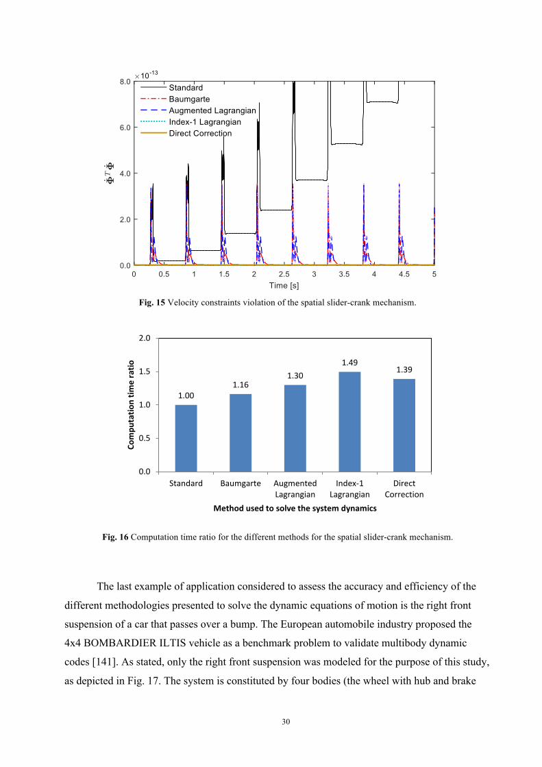
Figures 14 and 15 present the evolution of the constraints violation at the position and

velocity levels for the spatial slider-crank mechanism when different methods are utilized to

solve the dynamic equations of motion. From the analysis of the diagrams of these figures, it can

be drawn that when the standard Lagrange multipliers method is employed, the violation of the

constraint equations grows indefinitely with time. In reality, the standard approach based on the

Lagrange multipliers technique produces unacceptable results because the kinematic equations

are rapidly violated due to the inherent errors and instability that develop during computations.

In turn, with the stabilization methods, the system’s behavior is significantly different, in the

measure that the level of the constraints violation is kept under control during the computational

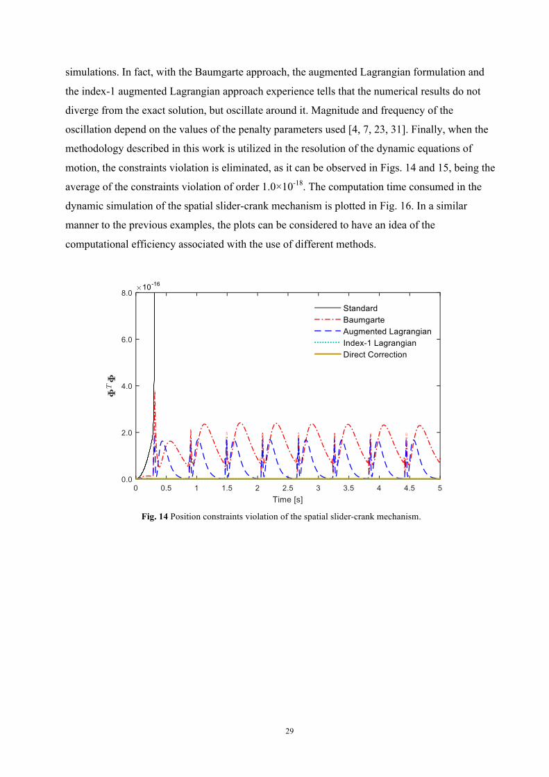
29

simulations. In fact, with the Baumgarte approach, the augmented Lagrangian formulation and

the index-1 augmented Lagrangian approach experience tells that the numerical results do not

diverge from the exact solution, but oscillate around it. Magnitude and frequency of the

oscillation depend on the values of the penalty parameters used [4, 7, 23, 31]. Finally, when the

methodology described in this work is utilized in the resolution of the dynamic equations of

motion, the constraints violation is eliminated, as it can be observed in Figs. 14 and 15, being the

average of the constraints violation of order 1.0×10-18. The computation time consumed in the

dynamic simulation of the spatial slider-crank mechanism is plotted in Fig. 16. In a similar

manner to the previous examples, the plots can be considered to have an idea of the

computational efficiency associated with the use of different methods.

Fig. 14 Position constraints violation of the spatial slider-crank mechanism.

30

Fig. 15 Velocity constraints violation of the spatial slider-crank mechanism.

1.001.16

1.301.49

1.39

0.0

0.5

1.0

1.5

2.0

Standard Baumgarte AugmentedLagrangian

Index-­‐1Lagrangian

DirectCorrection

Compu

tatio

n  tim

e  ratio

Method  used  to  solve  the  system  dynamics

Fig. 16 Computation time ratio for the different methods for the spatial slider-crank mechanism.

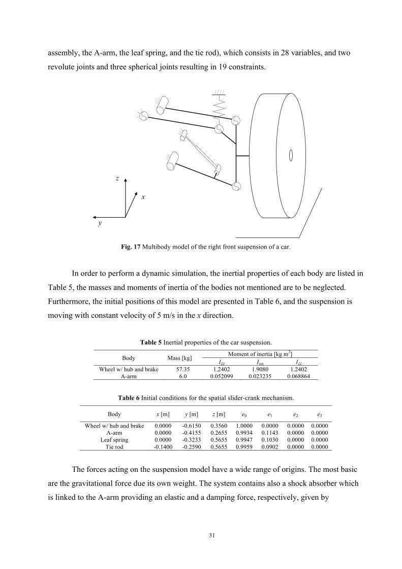
The last example of application considered to assess the accuracy and efficiency of the

different methodologies presented to solve the dynamic equations of motion is the right front

suspension of a car that passes over a bump. The European automobile industry proposed the

4x4 BOMBARDIER ILTIS vehicle as a benchmark problem to validate multibody dynamic

codes [141]. As stated, only the right front suspension was modeled for the purpose of this study,

as depicted in Fig. 17. The system is constituted by four bodies (the wheel with hub and brake

31

assembly, the A-arm, the leaf spring, and the tie rod), which consists in 28 variables, and two

revolute joints and three spherical joints resulting in 19 constraints.

y

x

z

Fig. 17 Multibody model of the right front suspension of a car.

In order to perform a dynamic simulation, the inertial properties of each body are listed in

Table 5, the masses and moments of inertia of the bodies not mentioned are to be neglected.

Furthermore, the initial positions of this model are presented in Table 6, and the suspension is

moving with constant velocity of 5 m/s in the x direction.

Table 5 Inertial properties of the car suspension.

Body Mass [kg] Moment of inertia [kg m2] Iξξ Iηη Iζζ

Wheel w/ hub and brake 57.35 1.2402 1.9080 1.2402 A-arm 6.0 0.052099 0.023235 0.068864

Table 6 Initial conditions for the spatial slider-crank mechanism.

Body x [m] y [m] z [m] e0 e1 e2 e3

Wheel w/ hub and brake 0.0000 -0.6150 0.3560 1.0000 0.0000 0.0000 0.0000 A-arm 0.0000 -0.4155 0.2655 0.9934 0.1143 0.0000 0.0000

Leaf spring 0.0000 -0.3233 0.5655 0.9947 0.1030 0.0000 0.0000 Tie rod -0.1400 -0.2590 0.5655 0.9959 0.0902 0.0000 0.0000

The forces acting on the suspension model have a wide range of origins. The most basic

are the gravitational force due its own weight. The system contains also a shock absorber which

is linked to the A-arm providing an elastic and a damping force, respectively, given by

32

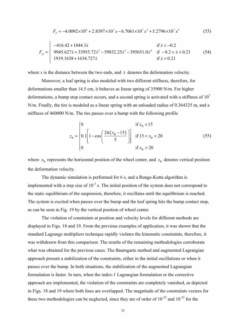
6 7 7 2 7 34.0092 10 2.8397 10 6.7061 10 5.2796 10SF x x x= − × + × − × + × (53)

FD =−416.42+1844.3 x if x < −0.29945.627 x + 33955.72 x2 −59832.25 x3 − 395651.0 x4 if − 0.2 < x < 0.211919.1638+1634.727 x if x > 0.21

⎧

⎨⎪

⎩⎪

(54)

where x is the distance between the two ends, and x denotes the deformation velocity.

Moreover, a leaf spring is also modeled with two different stiffness, therefore, for

deformations smaller than 14.5 cm, it behaves as linear spring of 35900 N/m. For higher

deformations, a bump stop contact occurs, and a second spring is activated with a stiffness of 107

N/m. Finally, the tire is modeled as a linear spring with an unloaded radius of 0.364325 m, and a

stiffness of 460000 N/m. The tire passes over a bump with the following profile

( )B

BB B

B

0 if 15

2 150.1 1 cos if 15 20

5

0 if 20

x

xz x

x

<⎧⎪ ⎡ ⎤π −⎛ ⎞⎪= − < <⎢ ⎥⎨ ⎜ ⎟

⎢ ⎥⎝ ⎠⎪ ⎣ ⎦⎪ >⎩

(55)

where Bx represents the horizontal position of the wheel center, and Bz denotes vertical position

the deformation velocity.

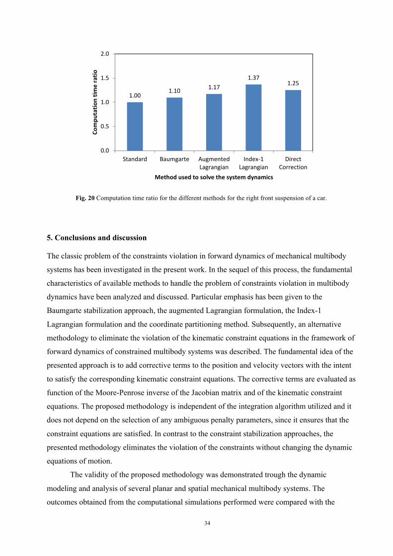
The dynamic simulation is performed for 6 s, and a Runge-Kutta algorithm is

implemented with a step size of 10-3 s. The initial position of the system does not correspond to

the static equilibrium of the suspension, therefore, it oscillates until the equilibrium is reached.

The system is excited when passes over the bump and the leaf spring hits the bump contact stop,

as can be seen in Fig. 19 by the vertical position of wheel center.

The violation of constraints at position and velocity levels for different methods are

displayed in Figs. 18 and 19. From the previous examples of application, it was shown that the

standard Lagrange multipliers technique rapidly violates the kinematic constraints, therefore, it

was withdrawn from this comparison. The results of the remaining methodologies corroborate

what was obtained for the previous cases. The Baumgarte method and augmented Lagrangian

approach present a stabilization of the constraints, either in the initial oscillations or when it

passes over the bump. In both situations, the stabilization of the augmented Lagrangian

formulation is faster. In turn, when the index-1 Lagrangian formulation or the corrective

approach are implemented, the violation of the constraints are completely vanished, as depicted

in Figs. 18 and 19 where both lines are overlapped. The magnitude of the constraints vectors for

these two methodologies can be neglected, since they are of order of 10-25 and 10-32 for the

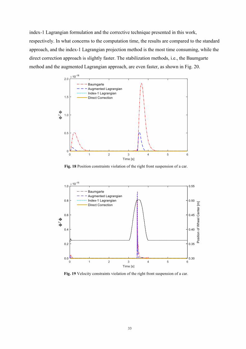
33

index-1 Lagrangian formulation and the corrective technique presented in this work,

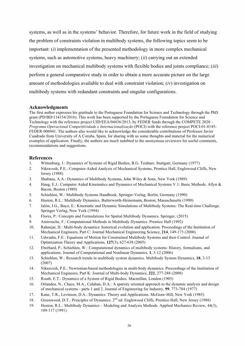
respectively. In what concerns to the computation time, the results are compared to the standard

approach, and the index-1 Lagrangian projection method is the most time consuming, while the

direct correction approach is slightly faster. The stabilization methods, i.e., the Baumgarte

method and the augmented Lagrangian approach, are even faster, as shown in Fig. 20.

Fig. 18 Position constraints violation of the right front suspension of a car.

Fig. 19 Velocity constraints violation of the right front suspension of a car.

34

1.001.10 1.17

1.371.25

0.0

0.5

1.0

1.5

2.0

Standard Baumgarte AugmentedLagrangian

Index-­‐1Lagrangian

DirectCorrection

Compu

tatio

n  tim

e  ratio

Method  used  to  solve  the  system  dynamics

Fig. 20 Computation time ratio for the different methods for the right front suspension of a car.

5. Conclusions and discussion The classic problem of the constraints violation in forward dynamics of mechanical multibody

systems has been investigated in the present work. In the sequel of this process, the fundamental

characteristics of available methods to handle the problem of constraints violation in multibody

dynamics have been analyzed and discussed. Particular emphasis has been given to the

Baumgarte stabilization approach, the augmented Lagrangian formulation, the Index-1

Lagrangian formulation and the coordinate partitioning method. Subsequently, an alternative

methodology to eliminate the violation of the kinematic constraint equations in the framework of

forward dynamics of constrained multibody systems was described. The fundamental idea of the

presented approach is to add corrective terms to the position and velocity vectors with the intent

to satisfy the corresponding kinematic constraint equations. The corrective terms are evaluated as

function of the Moore-Penrose inverse of the Jacobian matrix and of the kinematic constraint

equations. The proposed methodology is independent of the integration algorithm utilized and it

does not depend on the selection of any ambiguous penalty parameters, since it ensures that the

constraint equations are satisfied. In contrast to the constraint stabilization approaches, the

presented methodology eliminates the violation of the constraints without changing the dynamic

equations of motion.

The validity of the proposed methodology was demonstrated trough the dynamic

modeling and analysis of several planar and spatial mechanical multibody systems. The

outcomes obtained from the computational simulations performed were compared with the

35

results produced with the standard Lagrange multipliers technique, the Baumgarte stabilization

approach, the penalty method, the augmented Lagrangian formulation and the coordinate

partitioning method. The effectiveness of the methodology described in this work was analyzed

and compared in terms of constraints violation, conservation of the total energy and

computational efficiency. In a broad sense, it can be stated that the proposed approach is

effective in eliminate the constraints violation at both position and velocity levels without

penalizing the computational efficiency. With the described methodology, the energy of the

system can be over or under estimated because of the modifications associated with the

modifications of the positions and velocities constraints. This is a critical and open issue that can

be object of further investigation. The efficiency of the described method can be understood by

its nature, in the measure that the two-additional blocks are added to the standard solution of the

equations of motion. The elimination of the constraints violation for positions requires an

iterative procedure, because the corrective terms are dependent on the positions. However, based

on the computational tests performed, this process involves at most three iterations to eliminate

the constraints violation at the position to an acceptable level. In turn, the constraints violation

for velocities are eliminated with a single step, since constraints at the velocity level are linear

and the corrective terms are computed as function of the corrected positions performed

previously. Finally, it must be stressed that the described methodology is also effective to correct

the initial conditions, being the constraint equations satisfied to machine accuracy level.

Finally, it must be highlighted that some difficulties can arise when using the described

methodology. First of all, as it was presented previously, the computation of the generalized

inverse matrix expressed by Eq. (36) can be instable and highly cost. Alternative approaches to

deal with these issues have already been addressed in the literature [32, 39, 42, 90, 136-139]. On

the other hand, the process of correction of the positions and velocities by enforcing the

corresponding constraint equations does not require the use of a generalized inverse procedure,

but its particularization for the case of the minimum norm solution of a compatible undetermined

system of linear equations. This particular issue has been analyzed in detail in the seminal work

by Jalón and Gutiérrez-López [90]. Additionally, the described methodology can not handle the

problem associated with redundant constraints and inconsistency in the units utilized for the

coordinates and velocities [27, 78, 90, 103, 113]. Finally, in opposition to the coordinate

partitioning method, the described methodology refines the positions and velocity variables, by

means of Eqs. (41) and (49), nevertheless in the correction process they have missed the

consistency with the dynamic equations and the numerical integrator. This last issue can have

negative consequences in terms of the conservation of the total mechanical energy of the

36

systems, as well as in the systems’ behavior. Therefore, for future work in the field of studying

the problem of constraints violation in multibody systems, the following topics seem to be

important: (i) implementation of the presented methodology in more complex mechanical

systems, such as automotive systems, heavy machinery; (ii) carrying out an extended

investigation on mechanical multibody systems with flexible bodies and joints compliance; (iii)

perform a general comparative study in order to obtain a more accurate picture on the large

amount of methodologies available to deal with constraint violation; (iv) investigation on

multibody systems with redundant constraints and singular configurations.

Acknowledgments The first author expresses his gratitude to the Portuguese Foundation for Science and Technology through the PhD grant (PD/BD/114154/2016). This work has been supported by the Portuguese Foundation for Science and Technology with the reference project UID/EEA/04436/2013, by FEDER funds through the COMPETE 2020 – Programa Operacional Competitividade e Internacionalização (POCI) with the reference project POCI-01-0145-FEDER-006941. The authors also would like to acknowledge the considerable contributions of Professor Javier Cuadrado from University of A Coruña, Spain, for sharing with us some thoughts and material for the numerical examples of application. Finally, the authors are much indebted to the anonymous reviewers for useful comments, recommendations and suggestions.

References 1. Wittenburg, J.: Dynamics of Systems of Rigid Bodies, B.G. Teubner, Stuttgart, Germany (1977) 2. Nikravesh, P.E.: Computer-Aided Analysis of Mechanical Systems, Prentice Hall, Englewood Cliffs, New

Jersey (1988) 3. Shabana, A.A.: Dynamics of Multibody Systems, John Wiley & Sons, New York (1989) 4. Haug, E.J.: Computer Aided Kinematics and Dynamics of Mechanical Systems V.1: Basic Methods. Allyn &

Bacon, Boston (1989) 5. Schiehlen, W.: Multibody Systems Handbook, Springer-Verlag, Berlin, Germany (1990) 6. Huston, R.L.: Multibody Dynamics. Butterworth-Heinemann, Boston, Massachusetts (1990) 7. Jalón, J.G., Bayo, E.: Kinematic and Dynamic Simulations of Multibody Systems: The Real-time Challenge.

Springer Verlag, New York (1994) 8. Flores, P.: Concepts and Formulations for Spatial Multibody Dynamics. Springer, (2015) 9. Amirouche, F.: Computational Methods in Multibody Dynamics. Prentice Hall (1992) 10. Rahnejat, H.: Multi-body dynamics: historical evolution and application. Proceedings of the Institution of

Mechanical Engineers, Part C: Journal Mechanical Engineering Science, 214, 149-173 (2000) 11. Udwadia, F.E.: Equations of Motion for Constrained Multibody Systems and their Control. Journal of

Optimization Theory and Applications, 127(3), 627-638 (2005) 12. Eberhard, P., Schiehlen, W.: Computational dynamics of multibody systems: History, formalisms, and

applications. Journal of Computational and Nonlinear Dynamics, 1, 3-12 (2006) 13. Schiehlen, W.: Research trends in multibody system dynamics. Multibody System Dynamics, 18, 3-13

(2007) 14. Nikravesh, P.E.: Newtonian-based methodologies in multi-body dynamics. Proceedings of the Institution of

Mechanical Engineers, Part K: Journal of Multi-body Dynamics, 222, 277-288 (2008) 15. Routh, E.T.: Dynamics of a System of Rigid Bodies. Macmillan, London (1905) 16. Orlandea, N., Chace, M.A., Calahan, D.A.: A sparsity oriented approach to the dynamic analysis and design

of mechanical systems - parts 1 and 2. Journal of Engineering for Industry, 99, 773-784 (1977) 17. Kane, T.R., Levinson, D.A.: Dynamics: Theory and Applications. McGraw-Hill, New York (1985) 18. Greenwood, D.T.: Principles of Dynamics. 2nd ed. Englewood Cliffs, Prentice-Hall, New Jersey (1988) 19. Huston, R.L.: Multibody Dynamics – Modeling and Analysis Methods. Applied Mechanics Review, 44(3),

109-117 (1991)

37

20. Pfeifer, F., Glocker, C.: Multibody Dynamics with Unilateral Constraints. Wiley, New York (1996) 21. Nikravesh, P.E.: Planar Multibody Dynamics: Formulation, Programming, and Applications, CCR Press,

London (2008) 22. Guo, W., Wang, T.: A methodology for simulations of multi-rigid body systems with topology changes.

Multibody System Dynamics, 32(1), 25-38 (2015) 23. Nikravesh, P.E.: Some methods for dynamic analysis of constrained mechanical systems: A survey.

Computer-Aided analysis and Optimization of Mechanical System Dynamics, edited by E.J. Haug, Springer Verlag, Berlin, Germany, 351-368 (1984)

24. Rosen, A., Edelstein, E.: Investigation of a new formulation of the Lagrange method for constrained dynamic systems. Journal of Applied Mechanics, 64, 116-122 (1997)

25. Eich-Soellner, E., Führer, C.: Numerical Methods in Multibody Dynamics, vol. 45. Springer, Berlin (1998) 26. Von Schwerin, R.: Multibody System Simulation: Numerical Methods, Algorithms, and Software, vol. 7.

Springer, Berlin (1999) 27. Blajer, W.: Elimination of constraint violation and accuracy aspects in numerical simulation of multibody

systems. Multibody System Dynamics, 7, 265-284 (2002) 28. Laulusa, A., Bauchau, O.A.: Review of classical approaches for constraint enforcement in multibody

systems. J. Comput. Nonlinear Dyn. 3(1), 011004 (2007) 29. Bauchau, O.A., Laulusa, A.: Review of contemporary approaches for constraint enforcement in multibody

systems. J. Comput. Nonlinear Dyn. 3(1), 011005 (2007) 30. Masarati, P.: Constraint stabilization of mechanical systems in ordinary differential equations form.

Proceedings of the Institution of Mechanical Engineers, Part K: Journal of Multi-body Dynamics, 225, 12-33 (2011)

31. Flores, P., Machado, M., Seabra, E., Silva, M.T., A parametric study on the Baumgarte stabilization method for forward dynamics of constrained multibody systems. Journal of Computational and Nonlinear Dynamics, 6(1), 0110191-9 (2011)

32. Neto, M.A., Ambrósio, J.: Stabilization methods for the integration of DAE in the presence of redundant constraints. Multibody System Dynamics, 10, 81-105, (2003)

33. Fisette, P., Vaneghem, B.: Numerical integration of multibody system dynamic equations using the coordinate partitioning method in an implicit Newmark scheme. Computer Methods in Applied Mechanics and Engineering, 135, 85-105 (1996)

34. Ascher, U., Chin, H., Petzold, L., Reich, S.: Stabilization of constrained mechanical systems with DAEs and invariant manifolds. Mech. Struct. Mach. 23, 135-157 (1995)

35. Cuadrado, J., Cardenal, J., Bayo, E.: Modeling and solution methods for efficient real-time simulation of multibody dynamics. Multibody System Dynamics, 1(3), 259–280 (1997)

36. Schwerin, R.: Multibody System Simulation. Numerical Methods, Algorithms and Software. Springer, Berlin (1999)

37. Yu, Q., Chen, I.M.: A direct violation correction method in numerical simulation of constrained multibody systems. Comput. Mech. 26(1), 52-57 (2000)

38. Aghili, F., Piedbœuf, J.-C.: Simulation of motion of constrained multibody systems based on projection operator. Multibody System Dynamics, 10(1), 3-16 (2003)

39. Udwadia, F.E., Phohomsiri, P.: Explicit equations of motion for constrained mechanical systems with singular mass matrices and applications to multi-body dynamics. Proc. R. Soc. A, Math. Phys. Eng. Sci., 462(2071), 2097-2117 (2006)

40. Flores, P., Pereira, R., Machado, M., Seabra, E.: Investigation on the Baumgarte Stabilization Method for Dynamic Analysis of Constrained Multibody Systems. Edited by: Ceccarelli, M., Proceedings of the EUCOMES 08, The Second European Conference on Mechanism Science, Cassino, Italy, September 17-20, 2008, pp. 305-312 (2009)

41. Vlasenko, D., Kasper, R.: Implementation of consequent stabilization method for simulation of multibodies described in absolute coordinates. Multibody System Dynamics, 22, 297-319 (2009)

42. Mariti, L., Belfiore, N.P., Pennestrì, E., Valentini, P.P.: Comparison of solution strategies for multibody dynamics equations. Int. J. Numer. Methods Eng. 88(7), 637-656 (2011)

43. Müller, A.: Motion equations in redundant coordinates with application to inverse dynamics of constrained mechanical systems. Nonlinear Dynamics, 67, 2527-2541 (2012)

44. Uchida, T., Vyasarayani, C.P., Smart, M., McPhee, J.: Parameter identification for multibody systems expressed in differential-algebraic form. Multibody System Dynamics, 31(4), 393-403 (2014)

38

45. Baumgarte, J.: Stabilization of constraints and integrals of motion in dynamical systems. Computer Methods in Applied Mechanics and Engineering, 1, 1-16 (1972)

46. Baumgarte, J.: A New Method of Stabilization for Holonomic Constraints. Journal of Applied Mechanics, 50, 869-870 (1983)

47. Chang, C.O.: Dynamic Analysis and Optimum Design of Mechanical Systems with Constraint Violation Stabilization Method. Ph.D. Dissertation, Department of Mechanical Engineering, University of Iowa (1984)

48. Barzel, R., Barr, A.: A modeling system based on dynamic constraints. Computer Graphics, 22(4), 179-188 (1988)

49. Platt, J.C., Barr, A.: Constraint methods for flexible models. Computer Graphics, 22(4), 279-288 (1988) 50. Yoon, S.: Real-Time Simulation of Constrained Dynamic Systems. Ph.D. Dissertation, Department of

Aerospace Engineering, University of Michigan, Ann Arbor, MI (1990) 51. Ostermeyer, G.P.: On Baumgarte stabilization for differential algebraic equations, in: E.J. Haug, R.C. Deyo

(Eds.), Real-Time Integration Methods for Mechanical System Simulations, NATO ASI Series, Vol. F69, Springer, Berlin, 193-207 (1990)

52. Chin, H.S.: Stabilization Methods for Simulations of Constrained Multibody Dynamics. Ph.D. Dissertation, Department of Mathematics, The University of British Columbia, Canada (1995)

53. Eich, E., Hanke, M.: Regularization methods for constrained mechanical multibody systems. Zeitschrift fur angewandte Mathematik und Mechanik, 75(10), 761-773 (1995)

54. Baraff, D.: Linear-time dynamics using Lagrange multipliers. Proceedings of SIGGRAPH 1996, ACM Press/ACM SIGGRAPH, Computer Graphics Proceedings, 137-146 (1996)

55. Lin, S.T., Hong, M-C.: Stabilization method for numerical integration of multibody mechanical systems. Journal Mechanical Design, 120, 565-572 (1998)

56. Chiou, J.C., Wu, S.D.: Constraint violation stabilization using input-output feedback linearization in multibody dynamic analysis. Journal of Guidance, Control, and Dynamics, 21(2), 222-228 (1998)

57. Junkins, J.L., Akella, M.R., Kurdila, A.J.: Adaptive realization of desired constraint stabilization dynamics in the control of multibody systems. Philosophical Transactions: Mathematical, Physical & Engineering Sciences, 359(1788), 2231-2249 (2001)

58. Hajzman, M., Polach, P.: Application of stabilization techniques in the dynamic analysis of multibody systems. Applied and Computational Mechanics, 1, 479-488 (2007)

59. Machado, M., Costa, J., Seabra, E., Flores, P.: The effect of the lubricated revolute joint parameters and hydrodynamic force models on the dynamic response of planar multibody systems. Nonlinear Dynamics, 69(1-2), 635-654 (2012)

60. Ascher, U.R., Chin H., Reich, S.: Stabilization of DAEs and invariant manifolds. Numerische Methematik, 67(2), 131-149 (1994)

61. Chang, C.O., Nikravesh, P.E.: An adaptive constraint violation stabilization method for dynamic analysis of mechanical systems. Journal of Mechanisms, Transmissions, and Automation in Design, 107, 488-492 (1985)

62. Bae, D.S., Yang, S.M.: A stabilization method for kinematic and kinetic constraint equations. In E.J. Haug and R.C. Deyo, editors, Real-Time Integration Methods for Mechanical System Simulation, 209-232. Springer-Verlag, Berlin, Heidelberg, 1990.

63. Yoon, S., Howe, R.M., Greenwood, D.T.: Stability and accuracy analysis of Baumgarte’s constraint violation stabilization method. Journal of Mechanical Design, 117, 446-453 (1995)

64. Lin, S.T., Hong, M.C.: Stabilization method for numerical integration of multibody mechanical systems. Journal of Mechanical Design, 120, 565-572 (1998)

65. Lin, S-T., Huang, J-N.: Stabilization of Baumgarte’s method using the Runge-Kutta approach. Journal of Mechanical Design, 124, 633-641 (2002)

66. Park, K.C., Chiou, J.C.: Stabilization of computational procedures for constrained dynamical systems. Journal of Guidance, Control, and Dynamics, 11, 365-370 (1988)

67. Park, K.C., Chiou, J.C., Downer, J.D.: Explicit-implicit staggered procedure for multibody dynamics analysis. Journal of Guidance, Control, and Dynamics, 13(3), 562-570 (1990)

68. Ostermeyer, G.P.: On Baumgarte stabilization for differential algebraic equations. In E.J. Haug and R.C. Deyo, editors, Real-Time Integration Methods for Mechanical System Simulation, 193-207. Springer-Verlag, Berlin, Heidelberg (1990)

69. Yoon, S., Howe, R.M., Greenwood, D.T.: Constraint Violation Stabilization Using Gradient Feedback in Constrained Dynamics Simulation. Journal of Guidance, Control, and Dynamics, 15(6), 1467-1474 (1992)

39

70. Hong, M., Choi, M-H., Jung, S., Welch, S., Trapp, J.: Effective Constrained Dynamic Simulation Using Implicit Constraint Enforcement. Proceedings of the 2005 IEEE International Conference on Robotics and Automation, Barcelona, Spain, pp. 4531-4536 (2005)

71. Hong, M., Welch, S., Trapp, J., Choi, M.H.: Implicit Constraint Enforcement for Rigid Body Dynamic Simulation. Computational Science – ICCS 2006, Lecture Notes in Computer Science, 3991, 490-497 (2006)

72. Weijia, Z., Zhenkuan, P., Yibing, W.: An automatic constraint violation stabilization method for differential/algebraic equations on multibody system dynamics. Applied Mathematics and Mechanics, 21(1), 103-108 (2000)

73. Cline, M.B., Pai, D.K.: Post-Stabilization for Rigid Body Simulation with Contact and Constraints. In Proceedings of the IEEE International Conference on Robotics and Automation, 8p. (2003)

74. Bayo, E., Jalón, J.G., Serna, M.A.: A modified Lagrangian formulation for the dynamic analysis of constrained mechanical systems. Comput. Methods Appl. Math. 71(2), 183-195 (1988)

75. Bayo, E., Avello, A.: Singularity-free augmented Lagrangian algorithms for constrained multibody dynamics. Nonlinear Dynamics, 5(2), 209-231 (1994)

76. Terze, Z., Lefeber, D., Muftic, O.: Null Space Integration Method for Constrained Multibody Systems with No Constraint Violation. Multibody System Dynamics, 6, 229-243 (2001)

77. Braun, D.J., Goldfarb, M.: Eliminating constraint drift in the numerical simulation of constrained dynamical systems. Comput. Methods Appl. Math. 198(37–40), 3151–3160 (2009)

78. Blajer, W.: Methods for constraint violation suppression in the numerical simulation of constrained multibody systems - a comparative study. Comput. Methods Appl. Math. 200(13-16), 1568-1576 (2011)

79. Wehage, R.A., Haug, E.J.: Generalized coordinate partitioning for dimension reduction in analysis of constrained systems. Journal of Mechanical Design, 104, 247-255 (1982)

80. Nikravesh, P.E., Haug, E.J.: Generalized Coordinate Partitioning for Analysis of Mechanical System with Nonholonomic Constraints. Journal of Mechanisms, Transmissions, and Automation in Design, 105(3), 379-384 (1983)

81. Haug, E.J., Yen, J.: Generalized coordinate partitioning methods for numerical integration of differential-algebraic equations of dynamics. In Real-time Integration Methods for Mechanical System Simulation, Haug. E.J., Deyo. R.C. (eds). NATO ASI Series, Vol. 69. Springer, Berlin, 97-114 (1991)

82. Arabyan, A., Wu, F.: An improved formulation for constrained mechanical systems. Multibody Systems Dynamics, 2(1), 49-69 (1998)

83. Terze, Z., Naudet, J.: Geometric properties of projective constraint violation stabilization method for generally constrained multibody systems on manifolds. Multibody Systems Dynamics, 20, 85-106 (2008)

84. Terze, Z., Naudet, J.: Structure of optimized generalized coordinates partitioned vectors for holonomic and non-holonomic systems. Multibody Systems Dynamics, 24(2), 203-218 (2010)

85. Blajer, W., Schiehlen, W., Schirm, W.: A projective criterion to the coordinate partitioning method for multibody dynamics. Arch. Appl. Mech. 64, 86-98 (1994)

86. Nikravesh, P.E., Skinivasan, M.: Generalized co-ordinate partitioning in static equilibrium analysis of large-scale mechanical systems. Int. J. Numer. Methods Eng. 21, 451-464 (1985)

87. Jalón, J.G., Unda, J., Avello, A., Jiménez, J.M.: Dynamic analysis of three-dimensional mechanisms in natural coordinates. Computer Methods in Applied Mechanics and Engineering, 56, 309-327 (1986)

88. Ider, S.K., Amirouche, E.M.L.: Coordinate reduction in constrained spatial dynamic systems - a new approach. Journal of Applied Mechanics, 55, 899-905 (1988)

89. Fuhrer, C., Schwertassek, R.: Generation and solution of multibody systems equations. International Journal Non-Linear Mechanics, 25, 127-141 (1990)

90. Jalón, J.G., Gutiérrez-López, M.D.: Multibody dynamics with redundant constraints and singular mass matrix: existence, uniqueness, and determination of solutions for accelerations and constraint forces. Multibody System Dynamics, 30(3), 311-341 (2013)

91. Wehage, K.T., Wehage, R.A., Ravani, B.: Generalized coordinate partitioning for complex mechanisms based on kinematic substructuring. Mechanism and Machine Theory, 92, 464-483 (2015)

92. Carpinelli, M., Gubitosa, M., Mundo, D., Desmet, W.: Automated independent coordinates’ switching for the solution of stiff DAEs with the linearly implicit Euler method. Multibody System Dynamics, 36(1), 67-85 (2016)

93. Lubich, C.: Extrapolation integrators for constrained multibody systems. Impact Comput. Sci. Eng. 3(3), 213-234 (1991)

40

94. Andrzejewski, T., Bock, H.: Recent advances in the numerical integration of multibody systems. In: Schiehlen, W. (ed.) Advanced Multibody System Dynamics. Solid Mechanics and Its Applications, vol. 20, pp. 127-151. Springer, The Netherlands (1993)

95. Yu, Q., Chen, I.M.: A direct violation correction method in numerical simulation of constrained multibody systems. Computational Mechanics, 26(1), 52-57 (2000).

96. Eich, E.: Convergence results for a coordinate projection method applied to mechanical systems with algebraic constraints. SIAM J. Numer. Anal. 30(5), 1467-1482 (1993)

97. Yoon, S., Howe, R.M., Greenwood, D.T.: Geometric elimination of constraint violations in numerical simulation of Lagrangian equations. Journal of Mechanical Design, 116, 1058-1064 (1994)

98. Blajer, W.: An orthonormal tangent space method for constrained multibody systems. Computer Methods in Applied Mechanics and Engineering, 121, 45-57 (1995)

99. Blajer, W.: A geometric unification of constrained system dynamics. Multibody Syst. Dyn. 1(1), 3-21 (1997). 100. Aghili, F., Piedboeuf, J.C.: Simulation of motion of constrained multibody systems based on projection

operator. Multibody System Dynamics, 10(1), 3-16 (2003). 101. Tseng, F.-C., Ma, Z-D., Hulbert, G.M.: Efficient numerical solution of constrained multibody dynamics

systems. Computer Methods in Applied Mechanics and Engineering, 192, 439-472 (2003) 102. Nikravesh, P.E.: Initial condition correction in multibody dynamics. Multibody System Dynamics, 18:107-

115 (2007) 103. Zhang, J., Liu, D., Liu, Y.: A constraint violation suppressing formulation for spatial multibody dynamics

with singular mass matrix. Multibody System Dynamics, 36(1), 87-110 (2016) 104. Bayo, E., Ledesma, R.: Augmented Lagrangian and mass-orthogonal projection methods for constrained

multibody dynamics. Nonlinear Dynamics, 9(1-2), 113-130 (1996) 105. Orden, J.G.: Energy considerations for the stabilization of constrained mechanical systems with velocity

projection. Nonlinear Dynamics, 60(1-2), 49-62 (2010) 106. Orden, J.G., Conde Martín, S.: Controllable velocity projection for constraint stabilization in multibody

dynamics. Nonlinear Dyn. 68(1-2), 245-257 (2012) 107. Terze, Z., Müller, A. Zlatar, D.: Lie-group integration method for constrained multibody systems in state

space. Multibody System Dynamics, 34, 275-305 (2015) 108. Müller, A., Terze, Z.: The significance of the configuration space Lie group for the constraint satisfaction in

numerical time integration of multibody systems. Mechanism and Machine Theory, 82, 173-202 (2014) 109. Tian, Q., Xiao, Q., Sun, Y., Hu, H., Liu, H., Flores, P.: Coupling dynamics of a geared multibody system

supported by ElastoHydroDynamic lubricated cylindrical joints. Multibody System Dynamics, 33(3), 259-284 (2015)

110. Qi, Z., Wang, G., Zhang, Z.: Contact analysis of deep groove ball bearings in multibody systems. Multibody System Dynamics, 33(2), 115-141 (2015)

111. Blajer, W.: Augmented Lagrangian formulation: geometrical interpretation and application to systems with singularities and redundancy. Multibody System Dynamics 8(2), 141-159 (2002).

112. Haghshenas-Jaryani, M., Bowling, A.: A new switching strategy for addressing Euler parameters in dynamic modeling and simulation of rigid multibody systems. Multibody System Dynamics 30(2), 185-197 (2013)

113. Wojtyra, M., Fraczek, J.: Comparison of selected methods of handling redundant constraints in multibody system simulations. Journal of Computational and Nonlinear Dynamics, 8, 021007 (2013)

114. Unda, J., Jalón, J.G., Losantos, F., Emparantza, R.: A comparative study of different formulations of the dynamic equations of constrained mechanical systems. Journal of Mechanisms, Transmissions, and Automation in Design, 109, 466-474 (1987)

115. Udwadia, F.E., Kalaba, R.E.: A new perspective on constrained motion. Proc. R. Soc. Lond.,Math. Phys. Sci. 439(1906), 407-410 (1992)

116. Erberhard, P., Schielen, W.: Computational dynamics of multibody systems: history, formalisms, and applications. Journal of Computational and Nonlinear Dynamics, 1, 3-12 (2006)

117. Ruzzeh, B., Kövecses, J.: A penalty formulation for dynamic analysis of redundant mechanical systems. Journal of Computational and Nonlinear Dynamics, 6, 021008 (2011)

118. González, F., Kövecses, J.: Use of penalty formulations in the dynamic simulation and analysis of redundantly constrained multibody systems. Multibody System Dynamics, 29(1), 57-76 (2013)

119. Kim, J.K., Chung, I.S., Lee, B.H.: Determination of the Feedback Coefficients for the Constraint Violation Stabilization Method. Proceedings of the Institution of Mechanical Engineers, Part C: Journal of Mechanical Engineering Science, 204, 233-242 (1990)

41

120. Angles, J., Lee, S.: The formulation of dynamical equations of holonomic mechanical systems using a natural orthogonal complement. Journal of Applied Mechanics, 55, 243-244 (1988)

121. Agrawal, O.P., Saigal, S.: Dynamic analysis of multi-body systems using tangent coordinates. Computers & Structures, 31(3), 349-355 (1989)

122. Shabana, A.A.: Computational Dynamics. Wiley, New York (1994) 123. Jalón, J.G., Callejo, A., Hidalgo, A.F.: Efficient Solution of Maggi’s Equations. Journal of Computational

and Nonlinear Dynamics, 7(2), 021003 (2012) 124. Serban, R., Haug, E.J.: Globally Independent Coordinates for Real-Time Vehicle Simulation. Journal of

Mechanical Design, 122(4), 575-582 (2000) 125. Malczyk, P., Frączek, J.: A divide and conquer algorithm for constrained multibody system dynamics based

on augmented Lagrangian method with projections-based error correction. Nonlinear Dynamics, 70(1), 871-889, (2012)

126. Bayo, E., Jalón, J.G., Avello, A., Cuadrado, J.: An efficient computational method for real time multibody dynamic simulation in fully cartesian coordinates. Computer Methods in Applied Mechanics and Engineering, 92(3), 377-395 (1991)

127. Flores, P., Nikravesh, P.E.: Comparison of different methods to control constraints violation in forward multibody dynamics. Proceedings of the ASME Design Engineering Technical Conference, Volume 7 A. ASME 2013 International Design Engineering Technical Conferences and Computers and Information in Engineering Conference, IDETC/CIE 2013, Portland, OR, United States; 4-7 August, Code 103368 (2013)

128. Cuadrado, J., Cardenal, J., Morer, P., Bayo, E.: Intelligent simulation of multibody dynamics: Space–state and descriptor methods in sequential and parallel computing environments. Multibody System Dynamics, 4(1), 55-73, (2000)

129. Dopico, D., González, F., Cuadrado, J., Kövecses, J.: Determination of Holonomic and Nonholonomic Constraint Reactions in an Index-3 Augmented Lagrangian Formulation With Velocity and Acceleration Projections. Journal of Computational and Nonlinear Dynamics, 9(4), 041006, 9 pages (2014).

130. González, F., Dopico, D., Pastorino, R., Cuadrado, J.: Benchmarking of augmented Lagrangian and Hamiltonian formulations for multibody system dynamics. Proceedings of the ECCOMAS Thematic Conference on Multibody Dynamics June 29 - July 2, 2015, Barcelona, Catalonia, Spain, 1548-1559 (2015)

131. González, F., Dopico, D., Pastorino, R., Cuadrado, J.: Behaviour of augmented Lagrangian and Hamiltonian methods for multibody dynamics in the proximity of singular configurations. Nonlinear Dynamics, DOI: 10.1007/s11071-016-2774-5 (2016)

132. Flores, P.: A methodology for quantifying the position errors due to manufacturing and assemble tolerances. Journal of Mechanical Engineering, 57(6), 457-467 (2011)

133. Moore, E.H.: On the reciprocal of the general algebraic matrix. Bulletin of the American Mathematical Society, 26(9), 394-395 (1920)

134. Penrose, R.: A generalized inverse for matrices. Proceedings of the Cambridge Philosophical Society, 51, 406-413 (1955).

135. Rao, C.R., Mitra, S.K.: Generalized Inverse of Matrices and its Applications. John Wiley and Sons, New York (1971)

136. Mani, N.K., Haug, E.J.: Atkinson KE. Singular value decomposition for analysis of mechanical system dynamics. Journal of Mechanisms, Transmissions, and Automation in Design, 107, 82-87 (1985)

137. Singh, R.P., Likins. P.W.: Singular value decomposition for constrained mechanical systems. Journal of Applied Mechanics, 52, 943-948 (1985)

138. Kim, S.S., Vanderploeg, M.J.: QR decomposition for state space representation of constrained mechanical dynamical systems. Journal of Mechanisms, Transmissions, and Automation in Design, 108, 183-188, (1986)

139. Meijaard, J.P.: Applications of the single value decomposition in dynamics. Computer Methods in Applied Mechanics and Engineering, 103, 161-173 (1993)

140. McPhee, J., Shi, P., Piedbuf, J.-C.: Dynamics of Multibody Systems Using Virtual Work and Symbolic Programming. Mathematical and Computer Modelling of Dynamical Systems: Methods, Tools and Applications in Engineering and Related Sciences, 8(2), 137-155 (2002)

141. Iltis Data Package, IAVSD Workshop, Herbertov, Czechoslovakia, September 1990.