Filled Area Primitives

CEng 477Introduction to Computer Graphics

METU, 2007

Filled Area Primitives

● Two basic approaches to area filling on raster systems:

– Determine the overlap intervals for scan lines that cross the area (scan-line)

– Start from an interior position and point outward from this point until the boundary condition reached (fill method)

● Scan-line: simple objects, polygons, circles,..

● Fill-method: complex objects, interactive fill.

Polygon Fill Areas

● Most library routines require that a fill area be specified as a polygon

– OpenGL only allows convex polygons

● Non-polygon (curved) objects can be approximated by polygons

– Surface tessellation, polygon mesh, triangular mesh

Polygon types

● Simple polygon:

– all vertices are on the same plane and no edge crosses, no holes

simple polygonnot a simple polygon

Polygon types

● Simple polygons are either convex or concave:

– Convex polygon: All interior angles < 180°, or any line segment combining two points in the interior is also in the interior

convex polygon concave polygoncan be split into a number of convex polygons

Inside-Outside Tests

● Identifying the interior of a polygon (simple or complex) is important to identify the region to be filled

● Odd-even rule: To determine whether point P is inside or not. Draw a line starting from P to a distant position. Count the number of edges that crosses this line. If the count is odd then the point is inside, otherwise it is outside.

P

Front and Back Face of a Polygon

● The normal vector points in a direction from the back face of the polygon to the front face

● Normal vector is the cross product of the two edges of the polygon in counter- clockwise direction

)( 2312 V(V)VVN −×−=

N

V1

V2

V3

OpenGL Polygon Fill-Area Functions

● glRecti(50, 100, 200, 250)

50 100 150 200

100

150

200

250

50

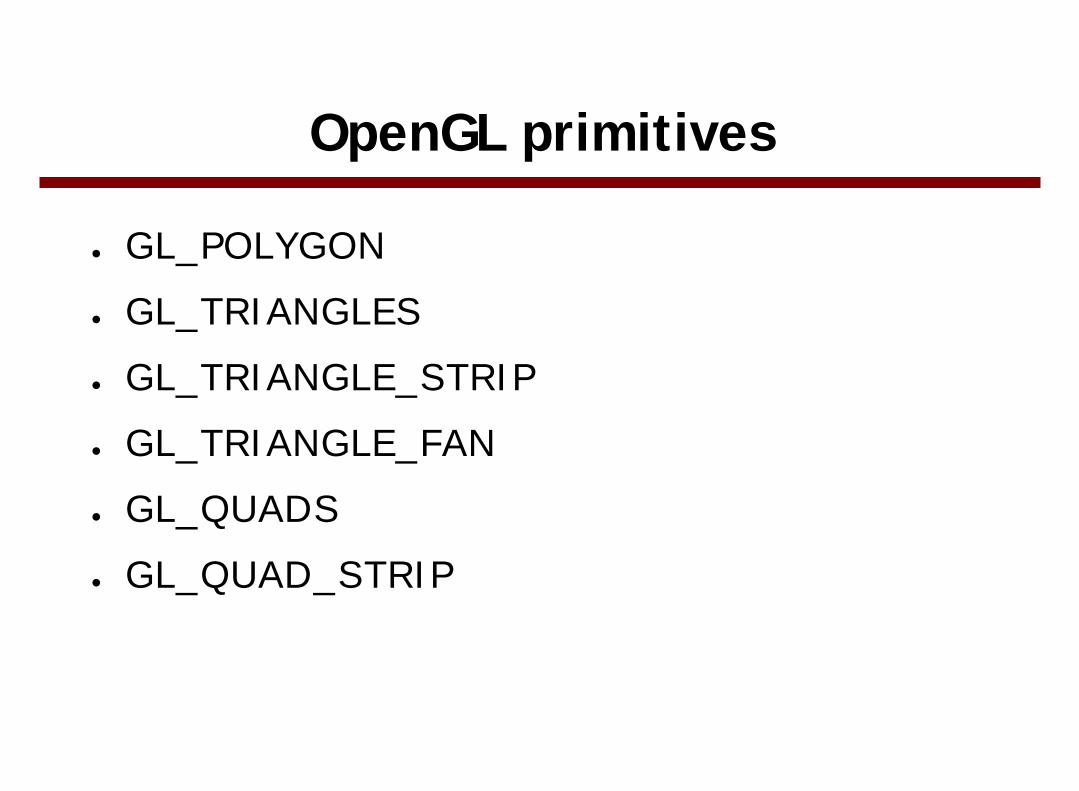
OpenGL primitives

● GL_POLYGON

● GL_TRIANGLES

● GL_TRIANGLE_STRIP

● GL_TRIANGLE_FAN

● GL_QUADS

● GL_QUAD_STRIP

OpenGL primitives

● GL_POLYGON

glBegin (GL_POLYGON);glVertex2iv (p1);glVertex2iv (p2);glVertex2iv (p3);glVertex2iv (p4);glVertex2iv (p5);glVertex2iv (p6);

glEnd ( );

p1

p2 p3

p4

p5p6

OpenGL primitives

● GL_TRIANGLES

glBegin (GL_TRIANGLES);glVertex2iv (p1);glVertex2iv (p2);glVertex2iv (p6);glVertex2iv (p3);glVertex2iv (p4);glVertex2iv (p5);

glEnd ( );

p1

p2 p3

p4

p5p6

OpenGL primitives

● GL_TRIANGLE_STRIP

glBegin (GL_TRIANGLE_STRIP);glVertex2iv (p1);glVertex2iv (p2);glVertex2iv (p6);glVertex2iv (p3);glVertex2iv (p5);glVertex2iv (p4);

glEnd ( );

p1

p2 p3

p4

p5p6

N vertices→N-2 trianglesorder of triangles: n, n+1, n+2 (if n is odd)

n+1, n, n+2 (if n is even) (n from 1 to N-2)

OpenGL primitives

● GL_TRIANGLE_FAN

glBegin (GL_TRIANGLE_FAN);glVertex2iv (p1);glVertex2iv (p2);glVertex2iv (p3);glVertex2iv (p4);glVertex2iv (p5);glVertex2iv (p6);

glEnd ( );

p1

p2 p3

p4

p5p6

N vertices→N-2 trianglesorder of triangles: 1, n+1, n+2

(n from 1 to N-2)

OpenGL primitives

● GL_QUADS

glBegin (GL_QUADS);glVertex2iv (p1);glVertex2iv (p2);glVertex2iv (p3);glVertex2iv (p4);glVertex2iv (p5);glVertex2iv (p6);glVertex2iv (p7);glVertex2iv (p8);

glEnd ( );

p1

p2 p3

p4 p5

p6p7

p8

OpenGL primitives

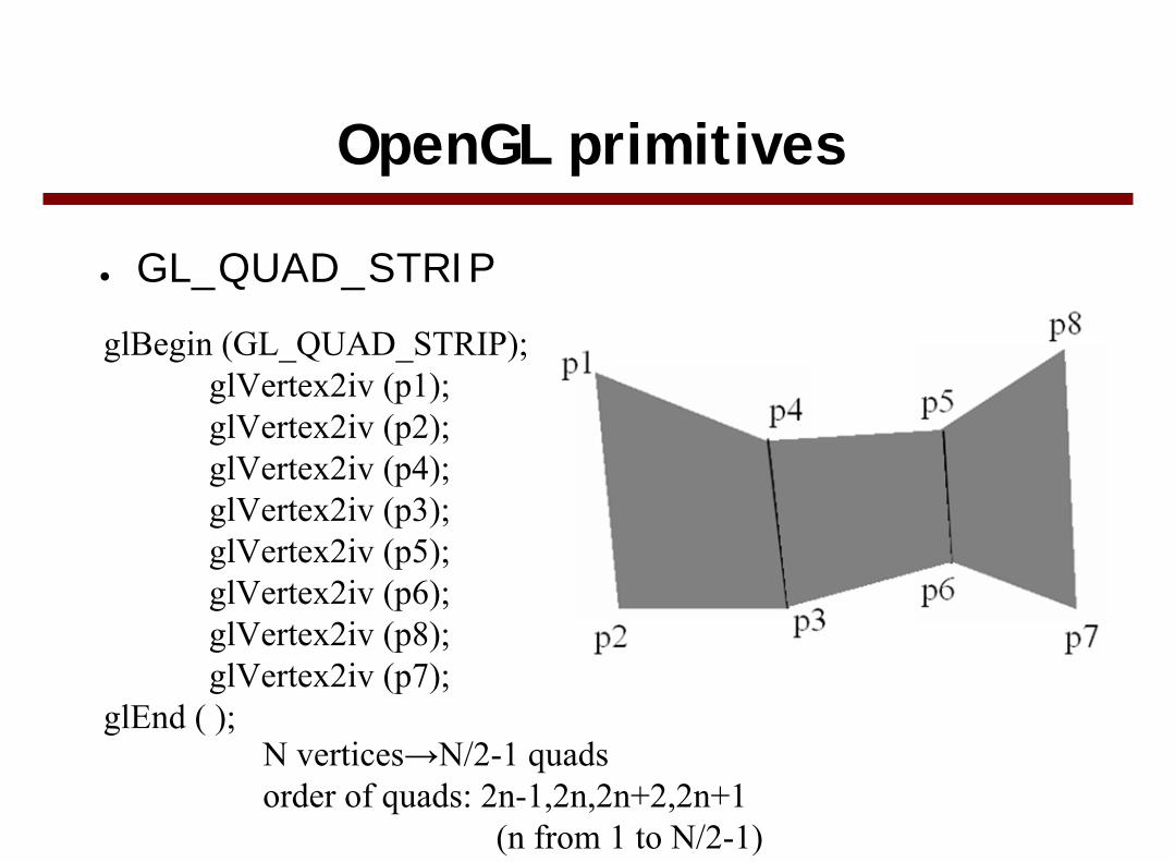
● GL_QUAD_STRIP

glBegin (GL_QUAD_STRIP);glVertex2iv (p1);glVertex2iv (p2);glVertex2iv (p4);glVertex2iv (p3);glVertex2iv (p5);glVertex2iv (p6);glVertex2iv (p8);glVertex2iv (p7);

glEnd ( );N vertices→N/2-1 quadsorder of quads: 2n-1,2n,2n+2,2n+1

(n from 1 to N/2-1)

OpenGL vertex arrays

● Complex scenes may require many glVertex() calls

● OpenGL provides vertex arrays to reduce function calls

● Drawing a cube:

glEnableClientState (GL_VERTEX_ARRAY);GLint pt[8][3] = {{0,0,0},{0,1,0},{1,0,0},{1,1,0},

{0,0,1},{0,1,1},{1,0,1},{1,1,1}};glVertexPointer (3, GL_INT, 0, pt);GLubyte vertIndex[24] ={6,2,3,7,5,1,0,4,7,3,1,5,4,0,2,6,2,0,1,3,7,5,4,6}; glDrawElements (GL_QUADS, 24, GL_UNSIGNED_BYTE, vertIndex);

OpenGL Display Lists

● Allows modular description of object components. Using display lists you can reference a set of OpenGL drawing commands multiple times

listID = glGenLists(1); // (number of list numbers to generate) glNewList (listID, GL_COMPILE_AND_EXECUTE); // or GL_COMPILE..........glEndList ( );

glCallList(listID);glDeleteLists(listID,1); // (startID, number of lists)

Fill Algorithms

● General Scan-Line Polygon fill algorithm

– to fill convex and concave polygons

● Boundary-Fill and Flood-Fill algorithms

– to fill arbitrary complex, irregular boundaries

● For now, assume that we fill the interior with a single color with no fill-pattern applied

● Application of fill-patterns is explained in sections 4-9 and 4-14 of your textbook

Scan-line Polygon Fill

● For each scan-line:

– Locate the intersection of the scan-line with the edges (y=ys )

– Sort the intersection points from left to right.

– Draw the interiors intersection points pairwise. (a-b), (c-d)

● Problem with corners. Same point counted twice or not?

a b c d

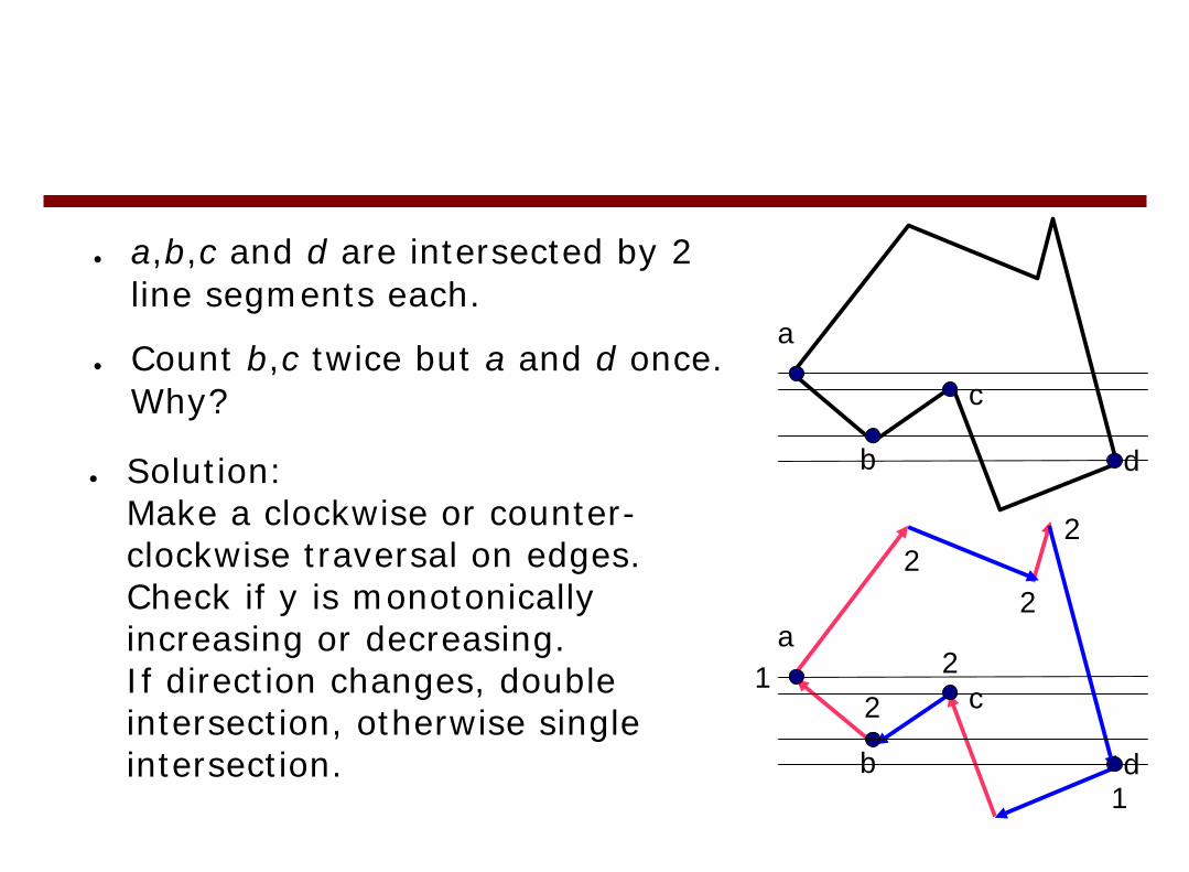
● a,b,c and d are intersected by 2 line segments each.

● Count b,c twice but a and d once. Why?

a

b

c

d

a

b

c

d

2

1

2

2

2

2

1

● Solution: Make a clockwise or counter- clockwise traversal on edges. Check if y is monotonically increasing or decreasing. If direction changes, double intersection, otherwise single intersection.

Scan-line Polygon Filling (coherence)

● Coherence: Properties of one part of a scene are related with the other in a way that can it be used to reduce processing of the other.

● Scan-lines adjacent to each other: The intersection points of edges with adjacent scan- lines are close to each other (like scan conversion of a line)

● Intersection points with scan lines:

xk 1 round xk1m

xk xk 1

yk 1

yk

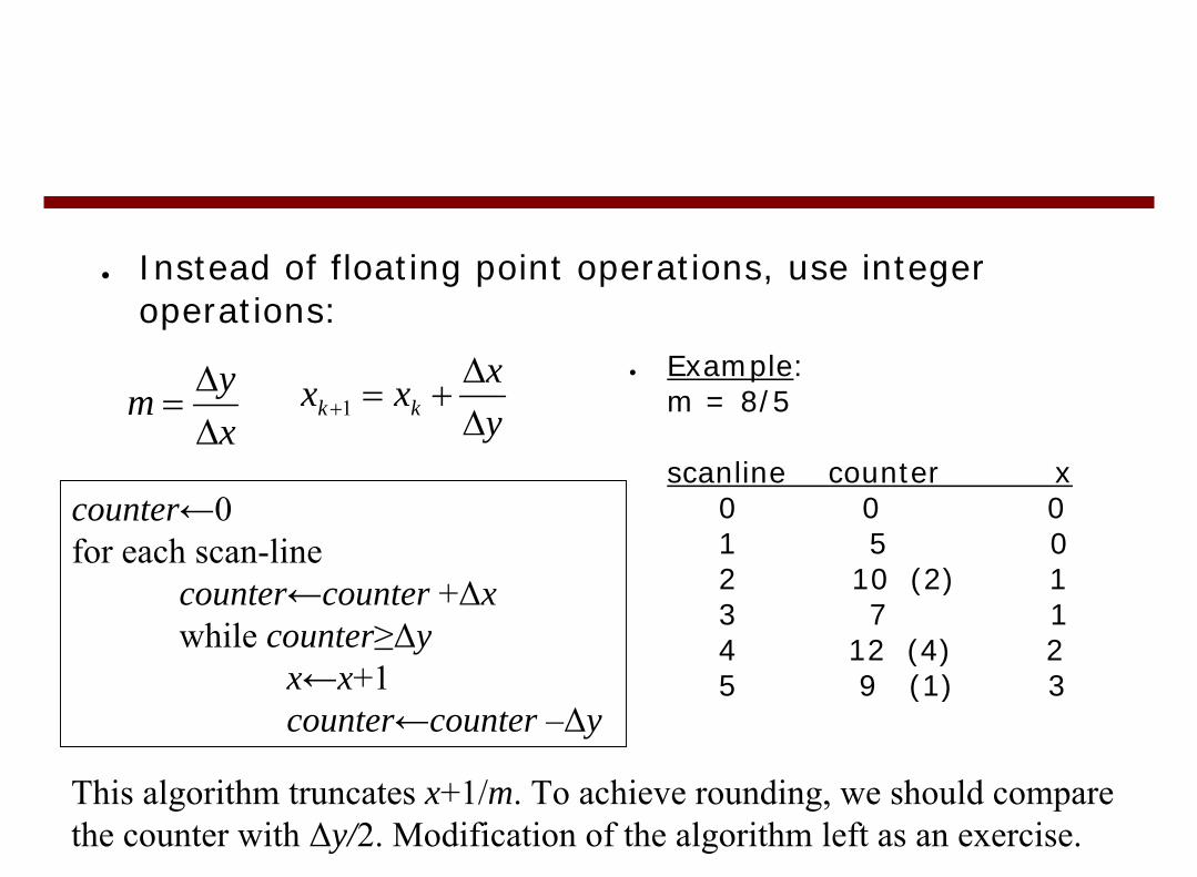
● Instead of floating point operations, use integer operations:

● Example: m = 8/5

scanline counter x 0 0 0 1 5 0 2 10 (2) 1 3 7 1 4 12 (4) 2 5 9 (1) 3

xym

ΔΔ

= yxxx kk Δ

Δ+=+1

counter←0for each scan-line

counter←counter +Δxwhile counter≥Δy

x←x+1counter←counter –Δy

This algorithm truncates x+1/m. To achieve rounding, we should comparethe counter with Δy/2. Modification of the algorithm left as an exercise.

Efficient Polygon Fill

● Make a (counter) clockwise traversal and shorten the single intersection edges by one pixel (so that we do not need to re-consider single/double edges).

● Generate a sorted edge table on the scan-line axis. Each edge has an entry in smaller y valued corner point (vertex).

● Each entry keeps a linked list of all connected edges:

– x value of the point

– y value of the end-point

– Slope of the edge

A

BD

C

E

E'

F

F'

yF' xA 1/mAF' yB xA 1/mAB

yE' xF 1/mFE'

yD xC 1/mCD yB xC 1/mCB

yD xE 1/mED

Scan line 01

Sorted edge table

● Start with the smallest scan-line

● Keep an active edge list:

– Update the current x value of the edge based on m value

– Add the lists in the current table entry based on their x value

– Remove the completed edges

– Draw the intermediate points of pairwise elements of the list.

● Example: A: (30,10),B: (24,32),C: (20,22), D: (16,34) E: (8,26), F: (12,16)

● Define the polygon with

A,B,C,D,E,F,A

Example

0

5

10

15

20

25

30

35

40

0 5 10 15 20 25 30 35

A

B

C

D

E

F

● Example: A: (30,10),B: (24,32),C: (20,22), D: (16,34) E: (8,26), F: (12,16)

● Define the polygon with

A,B,C,D,E,F,A

● E'=(20,25), F'=(12,15)

Sorted Edge Table: Y E1 E2 10 [15,30,-3] [32,30,-3/11] 16 [25,12,-2/5] 22 [34,20,-1/3] [32,20,2/5] 26 [34,8,1]

Example

0

5

10

15

20

25

30

35

40

0 5 10 15 20 25 30 35

A

B

C

D

E

F

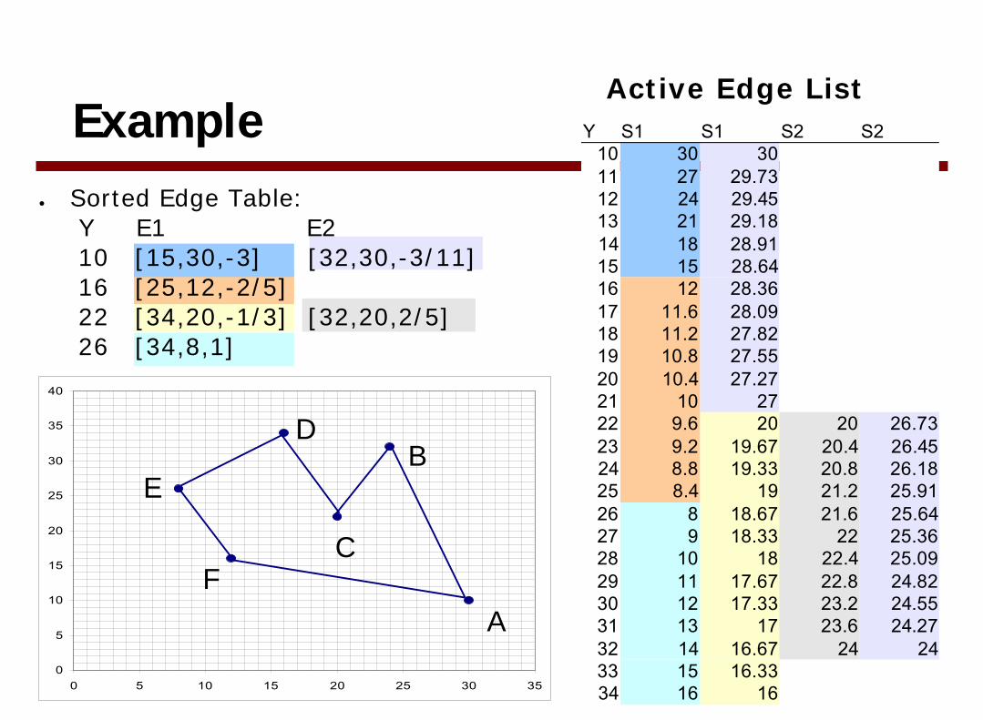
● Sorted Edge Table: Y E1 E2 10 [15,30,-3] [32,30,-3/11] 16 [25,12,-2/5] 22 [34,20,-1/3] [32,20,2/5] 26 [34,8,1]

Y S1 S1 S2 S210 30 3011 27 29.7312 24 29.4513 21 29.1814 18 28.9115 15 28.6416 12 28.3617 11.6 28.0918 11.2 27.8219 10.8 27.5520 10.4 27.2721 10 2722 9.6 20 20 26.7323 9.2 19.67 20.4 26.4524 8.8 19.33 20.8 26.1825 8.4 19 21.2 25.9126 8 18.67 21.6 25.6427 9 18.33 22 25.3628 10 18 22.4 25.0929 11 17.67 22.8 24.8230 12 17.33 23.2 24.5531 13 17 23.6 24.2732 14 16.67 24 2433 15 16.3334 16 16

Example

0

5

10

15

20

25

30

35

40

0 5 10 15 20 25 30 35

A

B

C

D

E

F

Active Edge List

Boundary Fill Algorithm● Start at a point inside a continuous arbitrary shaped

region and paint the interior outward toward the boundary. Assumption: boundary color is a single color

● (x,y): start point; b:boundary color, fill: fill color

void boundaryFill4(x,y,fill,b) { cur = getpixel(x,y) if (cur != b) AND (cur != fill) {

setpixel(x,y,fill); boundaryFill4(x+1,y,fill,b); boundaryFill4(x-1,y,fill,b); boundaryFill4(x,y+1,fill,b); boundaryFill4(x,y-1,fill,b);

} }

● 4 neighbors vs 8 neighbors: depends on definition of continuity. 8 neighbor: diagonal boundaries will not stop

● Recursive, so slow. For large regions with millions of pixels, millions of function calls.

● Stack based improvement: keep neighbors in stack

● Number of elements in the stack can be reduced by filling the area as pixel spans and pushing only the pixels with pixel transitions.

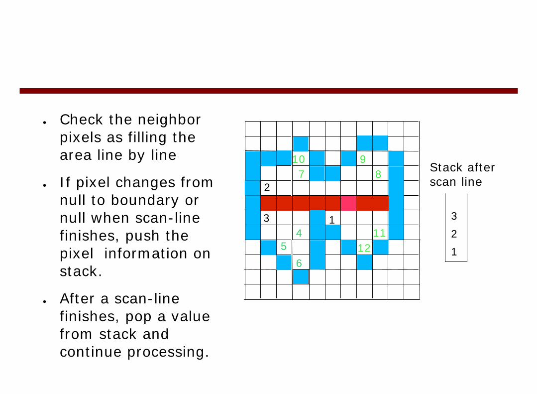
● Check the neighbor pixels as filling the area line by line

● If pixel changes from null to boundary or null when scan-line finishes, push the pixel information on stack.

● After a scan-line finishes, pop a value from stack and continue processing.

11

2

3

1

23

45

6

7 8910

1

12

Stack after scan line

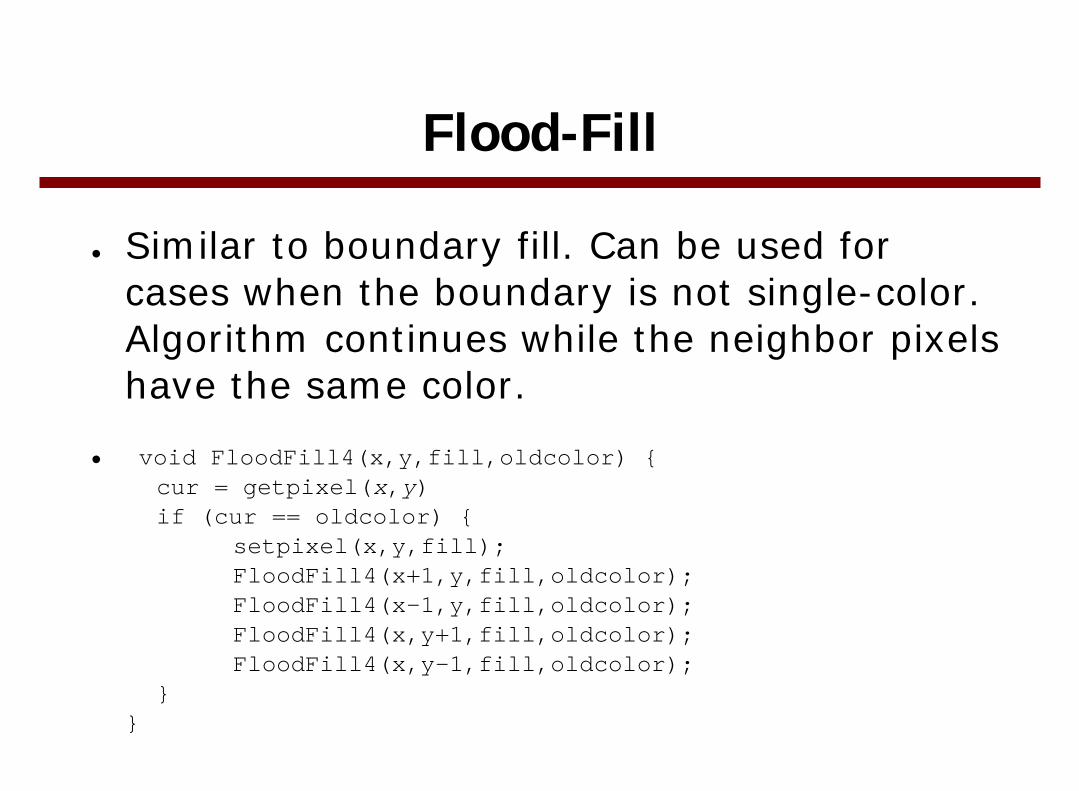
Flood-Fill

● Similar to boundary fill. Can be used for cases when the boundary is not single-color. Algorithm continues while the neighbor pixels have the same color.

● void FloodFill4(x,y,fill,oldcolor) { cur = getpixel(x,y) if (cur == oldcolor) {

setpixel(x,y,fill); FloodFill4(x+1,y,fill,oldcolor); FloodFill4(x-1,y,fill,oldcolor); FloodFill4(x,y+1,fill,oldcolor); FloodFill4(x,y-1,fill,oldcolor);

} }

Character Generation

● Typesetting fonts:

– Bitmap fonts: simple, not scalable.

– Outline fonts: scalable, flexible, more complex to process

● 0 0 0 0 0 0 0 0 0 0 0 1 1 1 0 0 0 0 1 1 0 1 1 0 0 1 1 0 0 0 1 1 0 1 1 0 0 0 1 1 0 1 1 1 1 1 1 1 0 1 1 1 1 1 1 1 0 1 1 0 0 0 1 1 0 1 1 0 0 0 1 1 0 1 1 0 0 0 1 1 0 1 1 0 0 0 1 1 0 0 0 0 0 0 0 0

Pixelwise on/of information

Points and tangents of the boundary