Filtering and Detrending

Fabio Canova

UPF and CEPR

December 2012

Outline

� Generics of trend/cycle decompositions.

� Standard decomposition: HP and Band pass �lters.

� Alternative decompositions: LT, SEGM, and FOD.

� Economic (VAR-based) decompositions.

� Statistical vs. economic �ltering.

� Collecting cyclical information

References

Baxter, M. and King, R., (1999), "Measuring Business Cycles: Approximate Band-Pass

Filters for Economic Time Series", Review of Economics and Statistics, 81, 575-593.

Beveridge, S. and Nelson, C., (1981), "A New Approach to Decomposition of Economic

Time Series into Permanent and Transitory Components with Particular Attention to the

Measurement of the Business Cycle", Journal of Monetary Economics, 7, 151-174.

Bry, G. and Boschen, C. (1971) Cyclical analysis of time series: Selected Procedures and

Computer Programs, New York, NBER

Canova, F., (1998), "Detrending and Business Cycle Facts", Journal of Monetary Eco-

nomics, 41, 475-540.

Canova, F., (1999), "Reference Cycle and Turning Points: A Sensitivity Analysis to

Detrending and Dating Rules", Economic Journal, 109, 126-150.

Canova, F., (2010), "Bridging DSGE models and the data", manuscript.

Canova, F., and Ferroni, F. (2011), "Multiple �ltering device for the estimation of DSGE

models", Quantitative Economics, 2, 37-59.

Chari, V. Kehoe, P. and McGrattan, E. (2008), " Are structural VAR with long run re-

strictions useful for developing business cycle theory? ", Journal of Monetary Economics,

55, 1337-1352.

Christiano, L. and J. Fitzgerard (2003) The Band Pass Filter, International Economic

Review, 44, 435-465.

Cogley, T. and Nason, J., (1995), "The E�ects of the Hodrick and Prescott Filter on

Integrated Time Series", Journal of Economic Dynamics and Control, 19, 253-278.

Harvey, A. and Jeager, A., (1993), "Detrending, Stylized Facts and the Business Cycles",

Journal of Applied Econometrics, 8, 231-247.

Hodrick, R. and Prescott, E., (1997), "Post-War US Business Cycles: An Empirical

Investigation", Journal of Money Banking and Credit, 29, 1-16.

King, R. and Rebelo, S., (1993), "Low Frequency Filtering and Real Business Cycles",

Journal of Economic Dynamics and Control, 17, 207-231.

King, R. Plosser, C., Stock, J. and Watson, M. (1991) "Stochastic Trends and Economic

Fluctuations", American Economic Review, 81, 819-840.

Marcet, A. and Ravn, M. (2001) "The HP �lter in Cross Country Comparisons", LBS

manuscript.

Pagan, A. and Harding, D. (2002), "Dissecting the Cycle: A Methodological Investiga-

tion", Journal of Monetary Economics, 49, 365-381.

Ravn, M and Uhlig, H. (2002), On adjusting the HP �lter for the frequency of Observa-

tions, Review of Economics and Statistics, 84, 371-375.

1 Introduction

� Data is trending (and has breaks); models typically stationary and builtto explain cyclical uctuations.

How do you match (calibrated) models and the data? Detrend/�lter.

- If detrend, which method do we use? Typically LT, Segm-LT, FOD

- If �lter, which �lter do we use? Typically HP, BP.

Questions:

- Detrending: deterministic or stochastic trend? With breaks or without?

- Filtering: which �lter? Which frequencies to keep? Filter all the data or

only real variables? Filter only actual data or actual and simulated data?

- Theories talk about permanent and transitory shocks. How do they relate

to statistical "trend" and "cycle" terms.

- How do we link "neutrality" propositions (e.g. long run money neutrality)

to "trend and cycle" decompositions?

General conundrums:

- What is the cycle? Macroeconomists: business cycle is the presence

variability, serial and cross correlation in time series. Time series econo-

metricians: business cycle is a peak in the spectral density at cyclical

frequencies. Alternatively, repetition of expansion/recession phases.

- How do one extract the cycle? Should one use a statistical approach or

an economic model to obtain it? Should one use univariate or multivariate

approaches?

2 Generics

Assume (for simplicity) that the "trend" is everything that it is not the

"cycle", i.e. yt = yxt + y

ct .

� Trend and Cycles are unobservable.

� Nature of the decompositions depends:

i) Properties (de�nition) of the trend.

ii) Correlation trend-cycle (call it �).

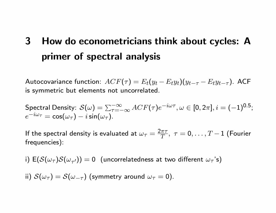
3 How do econometricians think about cycles: A

primer of spectral analysis

Autocovariance function: ACF (�) = Et(yt�Etyt)(yt�� �Etyt��). ACFis symmetric but elements not uncorrelated.

Spectral Density: S(!) = P�1�=�1ACF (�)e

�i!� ; ! 2 [0; 2�]; i = (�1)0:5;e�i!� = cos(!�)� i sin(!�).

If the spectral density is evaluated at !� =2��T ; � = 0; : : : ; T �1 (Fourier

frequencies):

i) E(S(!�)S(!� 0)) = 0 (uncorrelatedness at two di�erent !� 's)

ii) S(!�) = S(!��) (symmetry around !� = 0).

­π                                                           0 ω1 ω2 π

S(ω)

- Area under the spectral density is the variance of the process. Given or-

thogonality across frequencies (by 1. of previous slide), we can decompose

the variance into uncorrelated components.

- Value of the spectral density at frequency ! = 0 (=P�1�=�1ACF (�))

is a measure of the persistence of the process.

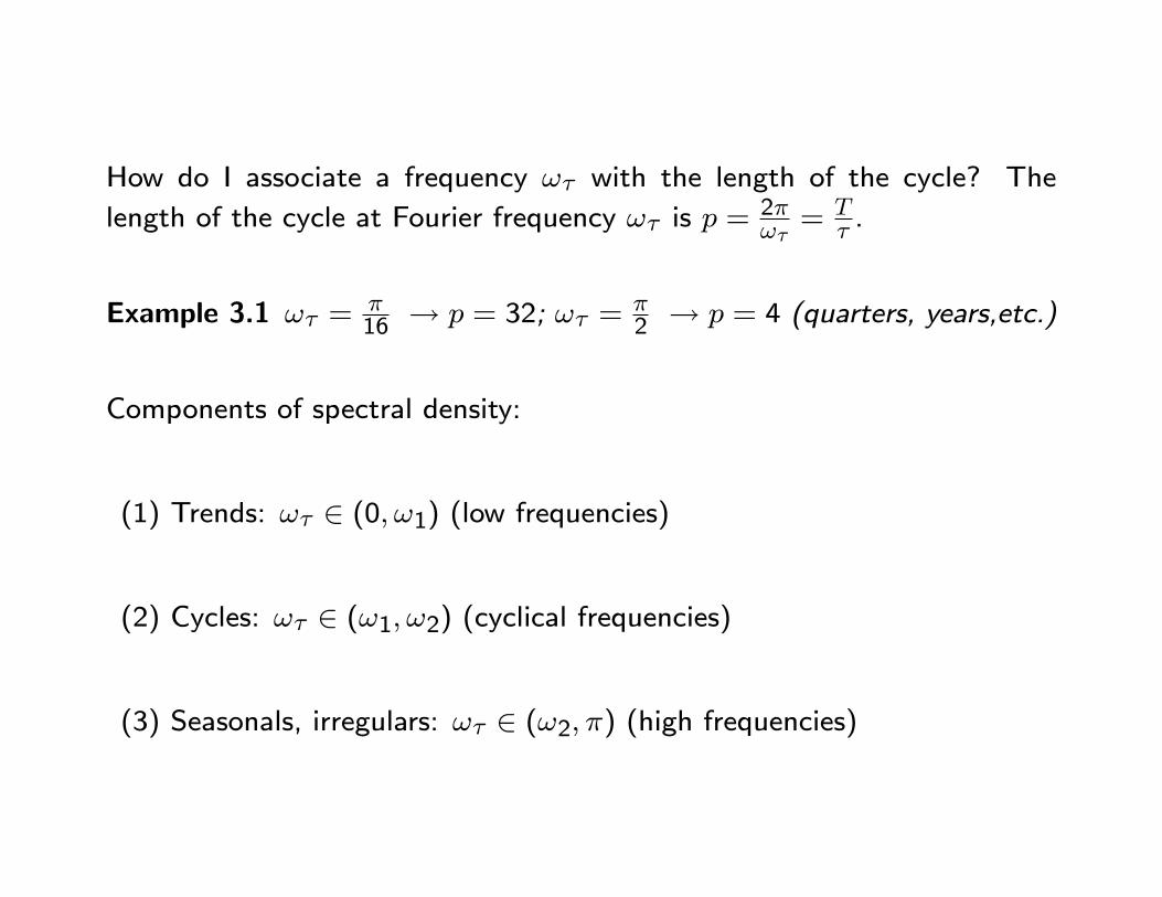
How do I associate a frequency !� with the length of the cycle? The

length of the cycle at Fourier frequency !� is p =2�!�= T

� .

Example 3.1 !� =�16 ! p = 32; !� =

�2 ! p = 4 (quarters, years,etc.)

Components of spectral density:

(1) Trends: !� 2 (0; !1) (low frequencies)

(2) Cycles: !� 2 (!1; !2) (cyclical frequencies)

(3) Seasonals, irregulars: !� 2 (!2; �) (high frequencies)

short periodicity

time

Am

plitu

re o

f cyc

les

0 50­1.0

­0.5

0.0

0.5

1.0 long periodicity

time

Am

plitu

re o

f cyc

les

0 50­1.0

­0.5

0.0

0.5

1.0

� Low frequencies (trends) are associated with long periods of oscillations(time series moves infrequently from peaks to throughs).

� High frequencies (irregulars) are associated with short cycles (time seriesmove frequently from peaks to throughs).

Examples of spectral densities

AR1

Fractions of pi0.0 0.2 0.4 0.6 0.8 1.0

0.01

0.10

1.00

10.00

100.00 MA1(negative)

Fractions of pi0.0 0.2 0.4 0.6 0.8 1.0

0.01

0.10

1.00

White noise

Fractions of pi0.0 0.2 0.4 0.6 0.8 1.0

0.01

0.10

1.00

AR2(complex)

Fractions of pi0.0 0.2 0.4 0.6 0.8 1.0

0.01

0.10

1.00

10.00

100.00

Conclusions:

- Displaying variability and serial correlation (e.g. AR(1) or MA(1) ) does

not generate cycles for econometricians. Need a AR(2) with complex roots.

- Having comovements: need to consider the spectral density matrix (see

appendix).

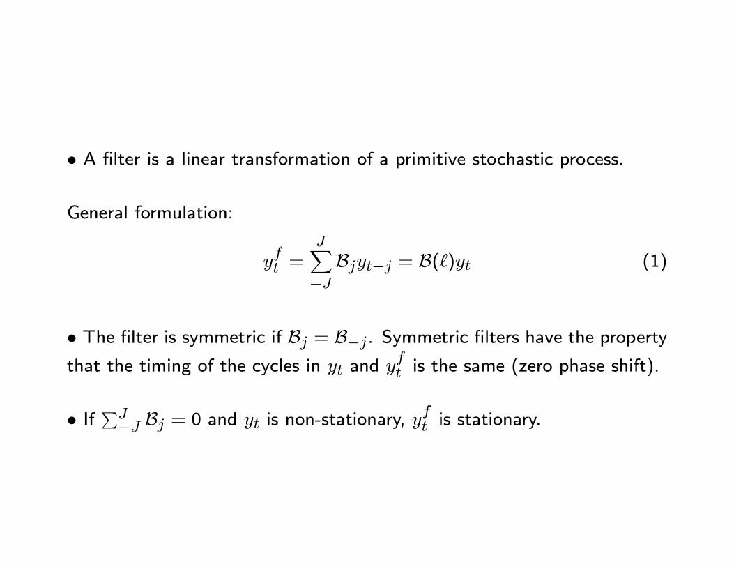
� A �lter is a linear transformation of a primitive stochastic process.

General formulation:

yft =

JX�JBjyt�j = B(`)yt (1)

� The �lter is symmetric if Bj = B�j. Symmetric �lters have the propertythat the timing of the cycles in yt and y

ft is the same (zero phase shift).

� If PJ�J Bj = 0 and yt is non-stationary, yft is stationary.

Terminology

� The frequency response function of the �lter is B(!) = B0+2Pj Bj cos(!j)

(i.e. set `j = ei!j); it measures the e�ect of a shock in yt on yft at fre-

quency !.

� jB(!)j is the gain function; it measures how much the amplitude of the uctuations y

ft changes relative to the amplitude of yt at frequency !.

� jB(!)j2 is the square gain; it measures how much the variance of yft

change relative to the variance of yt at frequency !.

4 The Hodrick and Prescott (HP) Filter

It solves the minimization problem:

minyxtfTXt=0

(yt � yxt )2 + �TXt=0

((yxt+1 � yxt )� (yxt � yxt�1))2g (2)

If � = 0 the solution is yxt = yt. As � "; yxt becomes smoother. If �!1,yxt becomes linear. Typically: � = 1600 for quarterly data.

Ravn and Uhlig (2002): if � = 129000 for monthly data and � = 6:25 for

annual data, HP picks cycles with similar periodicity for monthly, quarterly

and annual data.

Solution: yx = F�1HPy, yc = y� yx; y = [y1; : : : ; yT ]0; yxt = [yx1 ; : : : ; yxT ]

0,

FHP =

266666666666664

1 + � �2� 0 0 : : : : : : 0�2� 1 + 5� �4� 0 : : : : : : 0� �4� 1 + 6� �4� � : : : 00 � �4� 1 + 6� �4� : : : 0: : : : : : : : : : : : : : : : : : : : : : : :0 0 0 : : : 1 + 6� �4� �0 0 0 : : : �4� 1 + 5� �2�0 0 0 : : : 0 �2� 1 + �

377777777777775

HP �lter justi�ed:

- Literature on curve �tting (Wabha (1980)). Choose � to make MSE of

the �tting error minimal. In this case: �OPT =�2c�2x, where �2x (�

2c) is the

variance of the innovations in �2 trend (the cycle).

- Economic considerations: trends are smooth.

Solution:

- it is time dependent (the cycle at t depends on how large is T ).

- there are beginning and end-of-sample problems.

If we let �1 � t � 1, it can be shown that yct = yt � yxt = Bc(`)yt,where

Bc(`) ' (1� `)2(1� `�1)21� + (1� `)2(1� `�1)2

(3)

When � = 1600, the coe�cients of Bc(`) and the gain function jB(!)jlook like in the picture below.

Cyclical weights, lambda=1600

lags­50 0 50

­0.25

0.00

0.25

0.50

0.75

1.00Gain functions

frequency0.0 1.0 2.0 3.0

0.00

0.25

0.50

0.75

1.00

LAMBDA100LAMBDA400LAMBDA1600LAMBDA6400

Properties of HP �lter:

(i) It eliminates linear and quadratic trends from yt.

ii) It makes stationary series with up to 4 unit roots (King and Rebelo

(1993)).

What happens if the data has less than 4 unit roots? Overdi�erencing.

This means that we need a long AR speci�cation to represent yct .

- It can create spurious autocorrelation in �ltered series (Slutzky

e�ect).

Intuition: yt = et � iid(0; �2). Then

�yt = et � et�1 correlation of order 1

�2yt = et � et�1 � (et�1 � et�2) correlation of order 2; etc:

� Di�erencing a stationary process may induce spurious serial correla-tion in the di�erenced series.

Example 4.1 Consider a I(2) and a I(4) process and pass them through

a HP �lter. The �gure plots the ACF of the �ltered series. The serial

correlation in �ltered I(2) is higher then in the �ltered I(4).

5 10 15 20 25 30 35 40 45 50­0.50

­0.25

0.00

0.25

0.50

0.75

1.00I(0)I(2)I(4)

It can create spurious variability in the �ltered data.

If yt is stationary, the gain function is:

B(!) ' 16 sin4(!2 )1�+16 sin

4(!2 )=

4(1�cos(!))21�+4(1�cos(!))2

:

! it damps uctuations with periodicity � 24-32 quarters per cycle,

it passes short cycles without changes (similar to high pass �lter).

If yt is I(1) Bc(`) is a combination of two �lters: (1 � `) makes ytstationary,

B(`)1�` �lters �yt. When � = 1600 the gain function of

B(`)1�` is

' 2(1�cos(!))B(!), which peaks at !� = arccos[1� ( 0:751600)0:5] ' 30

periods:

y(t)~ I(0)

Frequency

HP

 filte

r

0.0 2.0

0.00

0.25

0.50

0.75

1.00

Frequency

ES fi

lter

0.0 2.5

0.00

0.25

0.50

0.75

1.00

y(t)~ I(1)

Frequency0.0 1.5 3.0

0

5

10

15

Frequency0.0 1.5 3.0

0

50

100

150

200

250

y(t)~ I(2)

Frequency0.0 1.5 3.0

0

100

200

300

400

Frequency0.0 2.0

0

100000

200000

300000

400000

! When applied to integrated quarterly data, HP damps long and

short run growth cycles and ampli�es growth cycles at business cycle

frequencies (e.g. the variance of the cycles with average duration of

7.6 years is multiplied by 13). Problem even larger if yt is I(2).

What if yt nearly integrated (�y = 0:95)? Same problem! (see dotted

line)

What is the intuition for the increased variability? Suppose �yt =

et � iid(0; �2). Then

var(�2yt) = var(et � et�1) = var(et) + var(et�1) = 2�2

var(�3yt) = var(et � 2et�1 + et�2) = 4�2

etc.. So the �lterB(`)1�` can augment the variability of �yt.

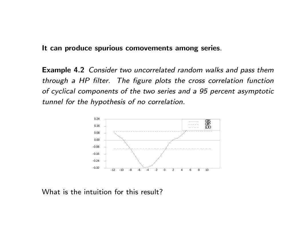
It can produce spurious comovements among series.

Example 4.2 Consider two uncorrelated random walks and pass them

through a HP �lter. The �gure plots the cross correlation function

of cyclical components of the two series and a 95 percent asymptotic

tunnel for the hypothesis of no correlation.

­12 ­10 ­8 ­6 ­4 ­2 0 2 4 6 8 10­0.32

­0.24

­0.16

­0.08

0.00

0.08

0.16

0.24 CRSUPPLOO

What is the intuition for this result?

The two �ltered series have similar spectrum. Therefore, it is possible

that they go up and down together (Note: this does not happen all

the times).

� The HP �lter has the potential to generate spurious variability,

spurious serial and cross variable correlations

iii) Other Problems:

- It is two sided; it may change in information set (impulse responses

may be incorrect).

- Leaves "undesirable" high frequency variability (it is a high pass

�lter).

- Cross county comparisons di�cult because cycles may have di�erent

length. Marcet-Ravn (2000) for international comparison assume that

the relative variability of the trend to the cycle is constant (i.e. series

in di�erent countries may have di�erent variabilities but the proportion

of trend variability to cycle variability is similar). In this case solve:

minyxt

TXt=1

(yt � yxt )2 (4)

V �PT�2t=1 (y

xt+1 � 2yxt + yxt�1)2PTt=1(yt � yxt )2

(5)

where V � 0 is a constant to be chosen by the researcher, V measuresthe relative variability of the acceleration in the trend and the cycle.

Example 4.3 200 data points from a stationary RBC model with utility

U(ct; ct�1; Nt) =c1�'t1�'+log(1�Nt) assuming � = 0:99; 'c = 2:0; � =

0:025; � = 0:64, steady state hours equal to 0.3, �� = 0:9; �g =

0:8; �� = 0:0066; �g = 0:0146. Table reports average unconditional

moments across 100 simulations, before and after HP �ltering.

Simulated statisticsRaw HP �ltered

K W LP K W LPcross (GDPt; xt) 0.49 0.65 0.09 0.84 0.95 -0.20cross (GDPt+1; xt) 0.43 0.57 0.05 0.60 0.67 -0.38St. Dev 1.00 1.25 1.12 1.50 0.87 0.50

� If HP �lter has problems, what else can we use?

5 Two sided (centered) or one-sided MA �lters.

Long history in business cycle analysis (Burns-Mitchell; Bry-Boschan).

yft =

JX�JBjyt�j = B(`)yt (6)

� Symmetric MA �lters (Bj = B�j) with limJ!1PJ�J Bj = 0 preferred

because they maintain lead/lag relationships and eliminate unit roots.

� HP is a symmetric, truncated MA �lter.

� What other �lters belong to the class of MA �lters?

Example 5.1 A symmetric (truncated) MA �lter is Bj = 12J+1; 0 � j �

jJ j and Bj = 0; j > jJ j.

If yct = (1�B(`))yt � Bc(`)yt the cyclical weights are Bc0 = 1�1

2J+1 and

Bcj = Bc�j = �1

2J+1, j = 1; 2 : : : ; J .

� Band Pass (BP) Filters

Combination of high pass and low pass MA �lters.

Low pass �lter: B(!) = 1 for j!j � !1 and 0 otherwise.

High pass �lter: B(!) = 0 for j!j � !1 and 1 otherwise.

Band pass �lter: B(!) = 1 for !1 � j!j � !2 and 0 otherwise.

 0 ω1 π             Low Pass

    1

    0

0 ω2 π       High Pass

    1

    0

  0 ω1 ω2 π           Band Pass

1

 0

Time series representation of the weights of the �lters:

Low pass: Blp0 =!1�; Blpj =

sin(j!1)j�

; 0 < j <1, some !1.

High pass: Bhp0 = 1� Blp0 ; Bhpj = �Blpj ; 0 < j <1.

Band pass: Bbp0 = Blpj (!2)� B

lpj (!1); 0 < j <1; !2 > !1.

� j must go to in�nity. Hence, these �lters are not realizable for T �nite.

Baxter and King (1994): for �nite T , cut at some �J <1.

- If the �lter is symmetric andP �J� �J BJ = 0 a truncated BP makes sta-

tionary series with quadratic trends and with up to two unit roots.

- BK approximation has the same problems of HP �lter if yt is (nearly)

integrated.

- J needs to be large for the approximation to be good, otherwise leakage

and compression.

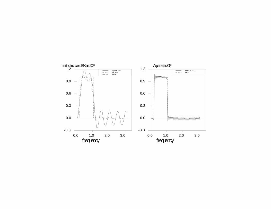
Symmetric truncated BK and CF

frequency0.0 1.0 2.0 3.0

­0.3

0.0

0.3

0.6

0.9

1.2 Sym­CF, J=12BK, J=12IDEAL

Asymmetric CF

frequency0.0 1.0 2.0 3.0

­0.3

0.0

0.3

0.6

0.9

1.2 Asym­CF, J=12IDEAL

- Christiano and Fitzgerald (2003): use a non-stationary, asymmetric ap-

proximation which is optimal in the sense of making the approximation

error as small as possible.

- In the solution, the coe�cients depend on time and change magnitude

and even sign with t.

- Better spectral properties (see picture) but:

a) Need to know the properties of time series before taking the approxi-

mation (need to know if it is a I(0) or I(1).

b) Phase shifts may occur.

- Christiano and Fitzgerald approximation is the same as Baxter and King

if yt is a white noise. In general, they will di�er.

6 Other �lters

� Polynominal trend, � = 0.

� Segmented linear trend, � = 0.

� RW trend, � = 0

Deterministic Polynomial Trend:

yxt = a+ bt+ ct2 + ::::

Estimate a; b; c; : : : in the regression

yt = a+ bt+ ct2 + ::::+ et

by OLS. Then set yct = yt � aOLS � bOLSt� cOLSt2 � : : :.

Problems:

- Can perfectly predict trend in the future.

- No acceleration/deceleration in the trend is possible.

- Unless estimates of a; b; c; : : : are obtained recursively, timing of informa-

tion in yct not necessarily the same as in yt (two-sided problem).

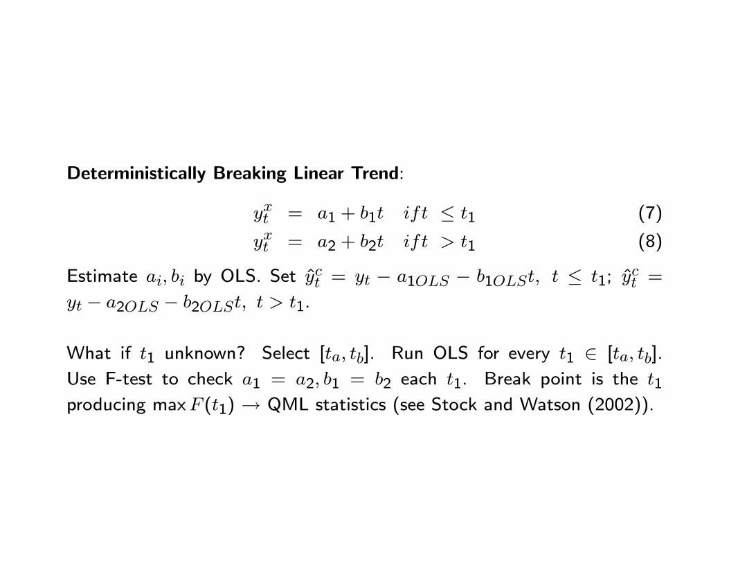
Deterministically Breaking Linear Trend:

yxt = a1 + b1t ift � t1 (7)

yxt = a2 + b2t ift > t1 (8)

Estimate ai; bi by OLS. Set yct = yt � a1OLS � b1OLSt; t � t1; y

ct =

yt � a2OLS � b2OLSt; t > t1.

What if t1 unknown? Select [ta; tb]. Run OLS for every t1 2 [ta; tb].

Use F-test to check a1 = a2; b1 = b2 each t1. Break point is the t1producing maxF (t1) ! QML statistics (see Stock and Watson (2002)).

Random Walk Trend, need yt to be I(1):

�yt = �yxt +�yct (9)

yxt = yxt�1 + et (10)

Estimate of the cyclical component: �yct = �yt � et � �yt.

� Potential problems:

- Growth rates very volatile. Di�cult to have models to explain them.

- Linearly detrended data still near nonstationary.

- Trade o�: larger samples/less stable estimates.

- Estimation results depend of the transformation used.

7 Economic (VAR based) Decompositions

- Filter actual and simulated data with the same (statistical) �lter. Com-

pute unconditional second moments and compare.

- Alternatives

i) Run a VAR on actual data and compute "structural" responses. Derive

population responses from the model. Compare the two (conditional sec-

ond moment comparison). Potential problem if estimated VAR is of small

dimension (Chari, Kehoe, McGrattan (2008)) or if data is short.

ii) Run a VAR on actual data. Compute "structural" responses. Simulate

data from the model of the same length as actual data. Run a VAR on sim-

ulated data. Compute "structural" responses using the same identi�cation

device. Compare them.

- Di�erence is that in ii) the VAR is an auxiliary model (we are not assuming

here that the model has a VAR representation). Similar in spirit to indirect

inference.

iii) Permanent-transitory decompositions (rather than trend-cycle decom-

positions).

- Blanchard and Quah (1989), trend random walk, � = 0.

- King, Plosser, Stock and Watson (1991), cointegrated trend, � = 0.

� Example of a BQ decomposition: Fisher's model

gdpt = gdpt�1 + a(�st � �st�1) + �st + �dt � �dt�1 (11)

unt = Nt �Nfe = ��dt � a�st (12)

d = demand, s = supply. This model implies that unt has no trend;

the trend in gdpt is gdpxt = gdpxt�1 + a(�st � �st�1); and the cycle is

gdpct = �dt � �dt�1 + �st .

- Supply shocks have long run e�ects on gdpt only.

- Both supply and demand shocks have cyclical e�ects on gdpt.

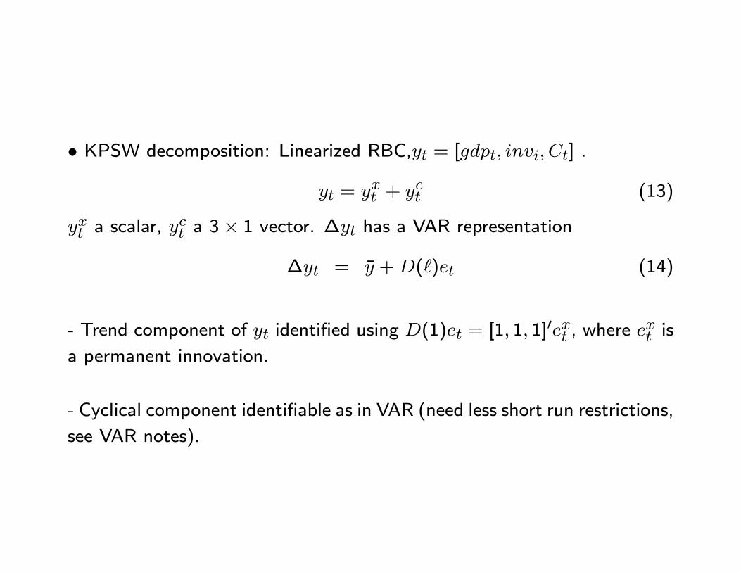
� KPSW decomposition: Linearized RBC,yt = [gdpt; invi; Ct] .

yt = yxt + y

ct (13)

yxt a scalar, yct a 3� 1 vector. �yt has a VAR representation

�yt = �y +D(`)et (14)

- Trend component of yt identi�ed using D(1)et = [1; 1; 1]0ext , where e

xt is

a permanent innovation.

- Cyclical component identi�able as in VAR (need less short run restrictions,

see VAR notes).

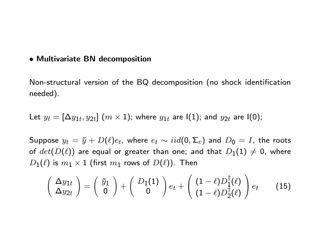
� Multivariate BN decomposition

Non-structural version of the BQ decomposition (no shock identi�cation

needed).

Let yt = [�y1t; y2t] (m� 1); where y1t are I(1); and y2t are I(0);

Suppose yt = �y + D(`)et, where et � iid(0;�e) and D0 = I, the roots

of det(D(`)) are equal or greater than one; and that D1(1) 6= 0, where

D1(`) is m1 � 1 (�rst m1 rows of D(`)). Then �y1t�y2t

!=

�y10

!+

D1(1)0

!et +

0@ (1� `)Dy1(`)(1� `)Dy2(`)

1A et (15)

is the multivariate BN decomposition, Dy1(`) =

D1(`)�D1(1)1�` D

y2(`) =

D2(`)1�` , 0 < rank[D1(1)] � m1 and �yxt = [�y1 +D1(1)et; 0]0 is the perma-nent component of yt.

Implementation:

i) Check unit roots and run a VAR yt = A(`)yt�1 + et

ii) Compute MA yt = D(`)et; D(`) = A(`)�1

iii) Trend is the constant plus the sum of MA coe�cients multiplied by the

shock; cycle is the rest.

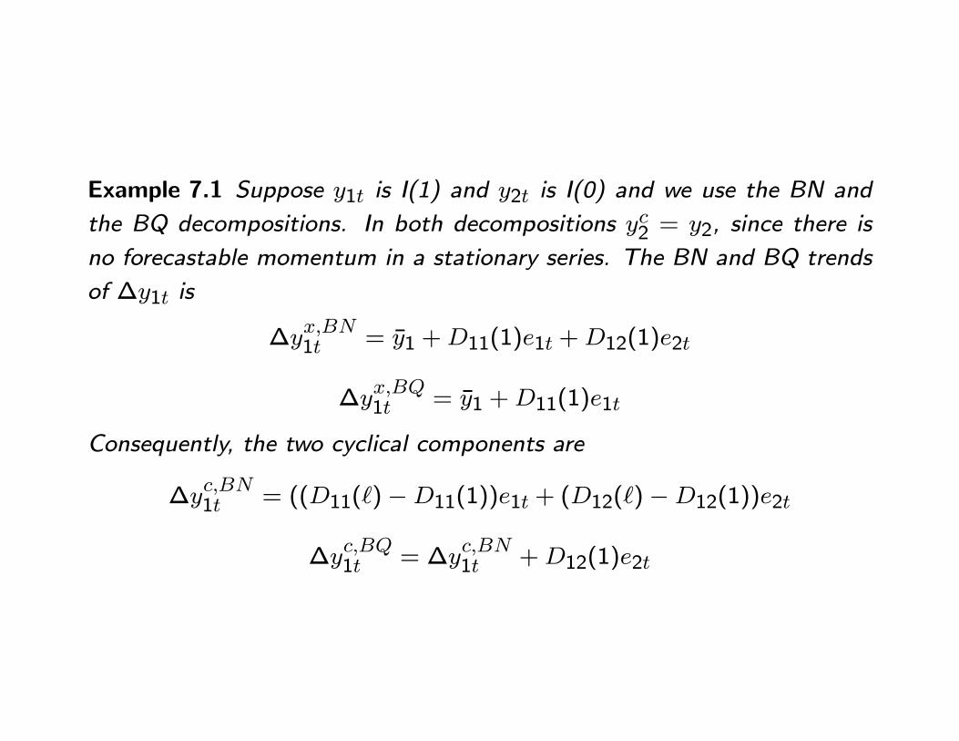
Example 7.1 Suppose y1t is I(1) and y2t is I(0) and we use the BN and

the BQ decompositions. In both decompositions yc2 = y2, since there is

no forecastable momentum in a stationary series. The BN and BQ trends

of �y1t is

�yx;BN1t = �y1 +D11(1)e1t +D12(1)e2t

�yx;BQ1t = �y1 +D11(1)e1t

Consequently, the two cyclical components are

�yc;BN1t = ((D11(`)�D11(1))e1t + (D12(`)�D12(1))e2t

�yc;BQ1t = �y

c;BN1t +D12(1)e2t

8 Economic vs. statistical �ltering

� Statistical �ltering: Find Bj such that yft has S(!�) 6= 0 only for certain

!� 2 (!1; !2).

� Economic �ltering: yt = y1t + y2t = A(L)et + B(L)ut, where et are

permanent shocks, ut are transitory shocks.

In general, y2t 6= yft since y2t has S(!�) 6= 0 for all !� 2 (0; �).

0 0.5 1 1.5 2 2.5 3 3.50

1000

2000

3000

4000

5000

6000

7000

8000

9000

10000Ideal Situation

datacycle 1

Ideal case

- (Cyclical) model has most of the variability located at business cycle

frequencies. Statistical �ltering ok.

0 0.5 1 1.5 2 2.5 3 3.50

1000

2000

3000

4000

5000

6000

7000

8000

9000

10000Cyclical has power outside BC frequencies

datacycle 2

Realistic case

- If the cyclical model is driven by persistent AR(1) shocks, time series

will have lots of variability in the low frequencies. Filtering throws away

information.

0 0.5 1 1.5 2 2.5 3 3.50

1000

2000

3000

4000

5000

6000

7000

8000

9000

10000Non­cyclical has power at BC frequencies

datacycle 3

General case

- If cyclical model is driven by persistent AR(1) shocks, and permanent

shocks have cyclical implications, �ltering is distortive. Di�erent �lters

will give di�erent results.

Typical solution: Forget statistical �ltering. Build in a trend in the model.

Transform the data with a model consistent approach. Problems:

- Models with trends (in technology) imply some balanced growth path.

Typically violated in the data (see next page).

- Where do we put the trend (e.g. technology or preferences) matters for

estimates of the structural parameters - nuisance parameter problem.

- Should we use a unit root or trend stationary speci�cation?

1950 : 1 1962 : 4 1975 : 1 1987 : 2 2000 : 10 . 55

0 . 6

0 . 65

G r e a t r a ti o s

c/y 

real

1950 : 1 1962 : 2 1975 : 1 1987 : 2 2000 : 10 . 05

0 . 1

0 . 15

0 . 2

i/y re

al

1950 : 1 1962 : 2 1975 : 1 1987 : 2 2000 : 10 . 5

0 . 6

0 . 7

c/y 

nom

inal

1950 : 1 1962 : 2 1975 : 1 1987 : 2 2000 : 10 . 05

0 . 1

0 . 15

0 . 2

i/y n

omin

al

0 0 .2 0 .4 0 .6 0 .8 1­ 2 0

­ 1 0

0

L o g  s p e c tr a

0 0 .2 0 .4 0 .6 0 .8 1­ 2 0

­ 1 0

0

0 0 .2 0 .4 0 .6 0 .8 1­ 2 0

­ 1 0

0

0 0 .2 0 .4 0 .6 0 .8 1­ 2 0

­ 1 0

0

Real and nominal Great ratios in US, 1950-2008.

Alternatives:

- Use a data rich environment (Canova and Ferroni, 2011).

- Bridge cyclical model and the data with a exible speci�cation for the

trend (Canova, 2010).

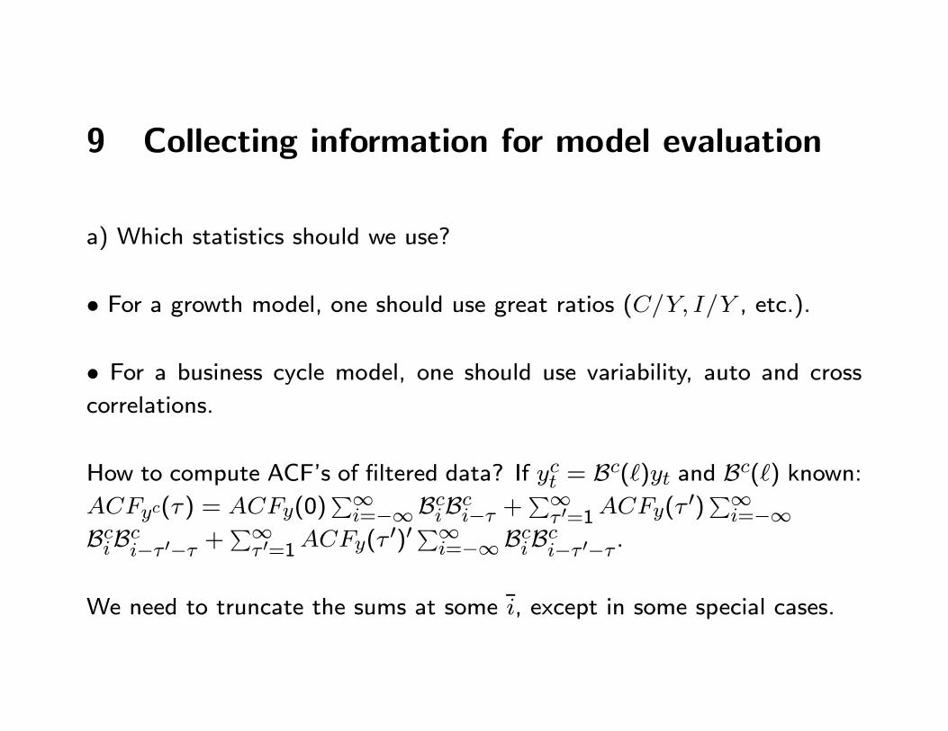
9 Collecting information for model evaluation

a) Which statistics should we use?

� For a growth model, one should use great ratios (C=Y; I=Y , etc.).

� For a business cycle model, one should use variability, auto and crosscorrelations.

How to compute ACF's of �ltered data? If yct = Bc(`)yt and Bc(`) known:ACFyc(�) = ACFy(0)

P1i=�1BciBci�� +

P1� 0=1ACFy(�

0)P1i=�1

BciBci�� 0�� +P1� 0=1ACFy(�

0)0P1i=�1BciBci�� 0�� .

We need to truncate the sums at some �i, except in some special cases.

b) Which �lter to use? Canova (1998, 1999): di�erent outcomes. Di�er-

ences due to:

� univariate vs multivariate decompositions

� orthogonal vs. non-orthogonal components

� carve di�erent portion of spectrum

� cyclical coe�cients di�erent

Summary statisticsVariability Relative Variability Contemporaneous Correlations Periodicity

Method GDP Consumption Real wage (GDP,C) (GDP,Inv) (GDP, W) (quarters)HP1600 1.76 0.49 0.70 0.75 0.91 0.81 24HP4 0.55 0.48 0.65 0.31 0.65 0.49 7BN 0.43 0.75 2.18 0.42 0.45 0.52 5BP 1.14 0.44 1.16 0.69 0.85 0.81 28KPSW 4.15 0.71 1.68 0.83 0.30 0.89 6

� Di�erences present also in other statistics, e.g. dating of cyclical turningpoints or measuring business cycle phases.

c) How do we choose cyclical frequencies? Use economic criteria?

- Within class of methods which roughly produce required cycles, di�er-

ences may emerge if series have spectral power concentrated in a neigh-

borhood of the trend/cycle cut-o� point (e.g Hours).

- Comparison across countries may be problematic.

- Filters may produce spurious periodicity and correlations.

- In developing countries trend may also be the cycle (Aguiar and Gopinath

(2007)) i.e. most of cyclical uctuations may be driven by permanent

shocks.

d) Pagan and Harding (2002): forget variability and ACF, use statistics

computable without knowing the time series properties of yt. How can you

do this? New Burns and Mitchell's (1946) approach.

Algorithm 9.1 1. Smooth yt to eliminate outliers, high frequency varia-

tions and other uninteresting uctuations. Call ysmt the smoothed series.

2. Determine a potential set of turning points using a rule like, e.g. �2ysmt >

0(< 0);�ysmt > 0(< 0);�ysmt+1 < 0(> 0);�2ysmt+1 < 0(> 0).

3. Use some criteria to ensure that peaks and troughs alternate and that

the duration and the amplitude of phases are meaningful.

Statistics one can compute:

- Average durations (AD), i.e. average length of time spent between peaksor between peaks and throughs.

- Average amplitudes (AA), i.e. the average size of the drop betweenpeaks and troughs or of the gain between troughs and peaks.

- concordance index CIj;j0 = n�1[P IjtIit � (1 � Ijt)(1 � Iit)]. Mea-

sures comovements over business cycle phases of two variables, where nis the number of complete cycles and Iit = 1 in expansions and Iit = 0in contractions (CI = 1(= 0) if the two series are perfectly positively(negatively) correlated).

- Average cumulative changes over phases (CM = 0:5 � (AD � AA))and excess average cumulative changes ECM = ((CM � CMA + 0:5 �AA)=AD), where CMA is the actual average cumulative change.

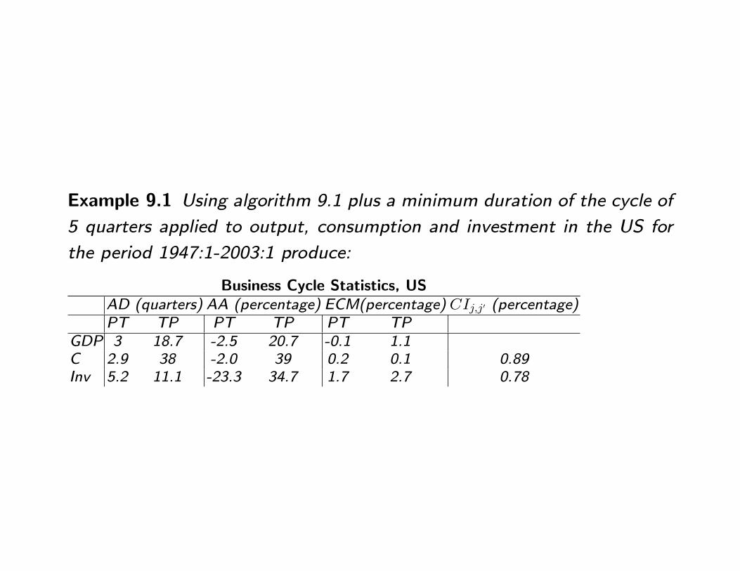
Example 9.1 Using algorithm 9.1 plus a minimum duration of the cycle of

5 quarters applied to output, consumption and investment in the US for

the period 1947:1-2003:1 produce:

Business Cycle Statistics, USAD (quarters) AA (percentage) ECM(percentage) CIj;j 0 (percentage)PT TP PT TP PT TP

GDP 3 18.7 -2.5 20.7 -0.1 1.1C 2.9 38 -2.0 39 0.2 0.1 0.89Inv 5.2 11.1 -23.3 34.7 1.7 2.7 0.78

- No need to extract cyclical components

- Collect cyclical features even if no (time series) cycles are present (good

for DSGE models which have no time series cycles).

- Results sensitive to dating rule [2.] and to minimum duration of phases

(Typically: two or three quarters - so that complete cycles should be at

least 5 to 7 quarters long) and to minimum amplitude restrictions (e.g.

peaks to troughs drops of less than one percent should be excluded).

- How to adapt procedure to international comparisons?

ACF statistics and turning point statistics are reduced form summary. But

DSGE models produce conditional statistics (impulse responses). How can

we use them?

10 Exercises

Exercise 1 Suppose yt = �yt�1 + et; et � (0; 1). Consider the �lter B(`) = 1� 2`+ `2and apply it yt. What are the properties of the �ltered series when � = 0:9? How does

the variability and the serial correlation in yft relate to those of yt.

Exercise 2 Suppose yt = et + �et�1; et � (0; 1). Consider the �lter B(`) = 1=3`�1 +1=3 + 1=3` and apply it yt. What are the properties of the �ltered series when � = 0:2?

How does the variability and the serial correlation in yft relate to those of yt.

Exercise 3 Suppose y1t is I(1) and y2t is I(0) and we use the BN and the BQ decompo-sitions. Calculate the BN and the BQ trends and show how the cyclical components ofthe two �lters are related.

Exercise 4 Simulate 11000 data points from yt = 0:9yt�1 + ut where ut iid(0; 1) fromy0 = 0 and throw away the �rst 1000 data points.1) Pass the series through Hodrick and Prescott �lter.2) Sample the series one every four (you will have in the end 2500 data points) and callthe sampled series xt. Calculate (by simulation) the value of � needed for the varianceof the HP �ltered xt to be the same as the variance of the HP �ltered yt.

3) Repeat the exercise in 2) using the �rst order autorrelation of xt and yt. How do the�'s obtained in 2) and 3) compare?

Exercise 5 Simulate 11000 data points from yt = 0:9yt�1 + ut where ut iid(0; 1) fromy0 = 0 and throw away the �rst 1000 data points. Pass the series through the followingMA �lters:a) Two sided symmetric J=4, equal weights summing to 1b) Two sided symmetric J=12, equal weights summing to 1c) One sided, backward, J=12, declining weights ((1=(j + 1))=(

Pj(1=(j + 1))); j =

0; 1; :::; 11)Compare the cyclical properties of the �ltered data obtained with the three �lters andcomment on the di�erences.

Appendix: Other elements of Spectral Analysis

The spectral density matrix of m� 1 vector fytg1t=�1 is

S(!) = 12�

P� ACF (�) exp(�i!�) where

S(!) =

264 Sy1y1(!) Sy1y2(!) : : : Sy1ym(!)Sy2y1(!) Sy2y2(!) : : : Sy2ym(!): : : : : : : : : : : :

Symy1(!) Symy2(!) : : : Symym(!)

375

Diagonal of the spectral density matrix real; o�-diagonal complex.

� The coherence between y1t and y2t is Coy1;y2(!) =jSy1;y2(!)j

(Sy1;y1(!)Sy2;y2(!))0:5.

It measures the strength of the association between two time series at frequency !. Note

thatRCo(!)d! = �y1;y2. Co(!) is real since jyj = real part of complex number y.

A few examples of �lters

Example 10.1 1) yt = et +D1et�1. yt is a �ltered version of et.

2) yt =PJj=�J et�j.

If CGFe(z) is the covariance generating function of et, yt = B(`)et the co-variance generating function of yt is CGFy(z) = B(z)B(z�1)CGFy(z) =jB(z)j2CGFy(z) where jB(z)j is the real part (modulus) of B(z).

Example 10.2 Let et be a white noise. Its spectrum is Se(!) = �2

2� . Let

yt = a(`)et where a(`) = a0 + a1` + a2`2 + : : : The spectrum of yt is

Sy(!) = ja(e�i!)j2Se(!) where ja(e�i!)j2 = a(e�i!)a(ei!).

� The periodogram of yt is Pe(!) =P�\ACF (�)e�i!� where\ACF (�) =

1T

Pt(yt � �y)(yt�� � �y) and �y = 1

T

Pt yt.

Periodogram is inconsistent estimator of the spectrum (periodogram con-

sistently estimate only an average of the frequencies of the spectrum. For

consistent estimates need to "smooth" periodogram with a �lter (kernel).

� A �lter is a kernel (denoted by KT (!)) if, as T ! 1, K(!�) =1; for !� = ! and K(!�) = 0 otherwise.

Kernels eliminate bias in\ACF (�). Since as T !1 bias disappears, wants

kernels to converge to ��function as T !1.

Two useful Kernels: "Bartlett " and the "quadratic spectral ".

- Bartlett: tent shaped, width 2J(T ); K(!j) = 1�j!jJ(T )

. J(T ) chosen so

thatJ(T )T ! 0 as T !1.

- Quadratic spectral kernel: wave with in�nite loops;

K(!j) = 2512�2j2

sin(6�j=5)(6�j)=5

� cos(6�j5 ).

­20 ­10 0       10        20 ω               Bartlett Kernel

κ(ω)

    1

    0

­20 ­10 0       10        20 ω                Quadratic Spectral Kernel

κ(ω)

    1

    0