filtering and edge detection - princeton university
TRANSCRIPT

Image Analysis

Motivation
Computer vision
Input: digital images
Output: information about the world

Image Analysis
Input is a regular array of discrete samples of a
2D continuous function representing color
Output is info about
structure of image
Color image
e.g., Color at (x,y)

Image Analysis
For now, let’s consider only gray-level images
e.g., Luminance at (x,y)
Gray-level image
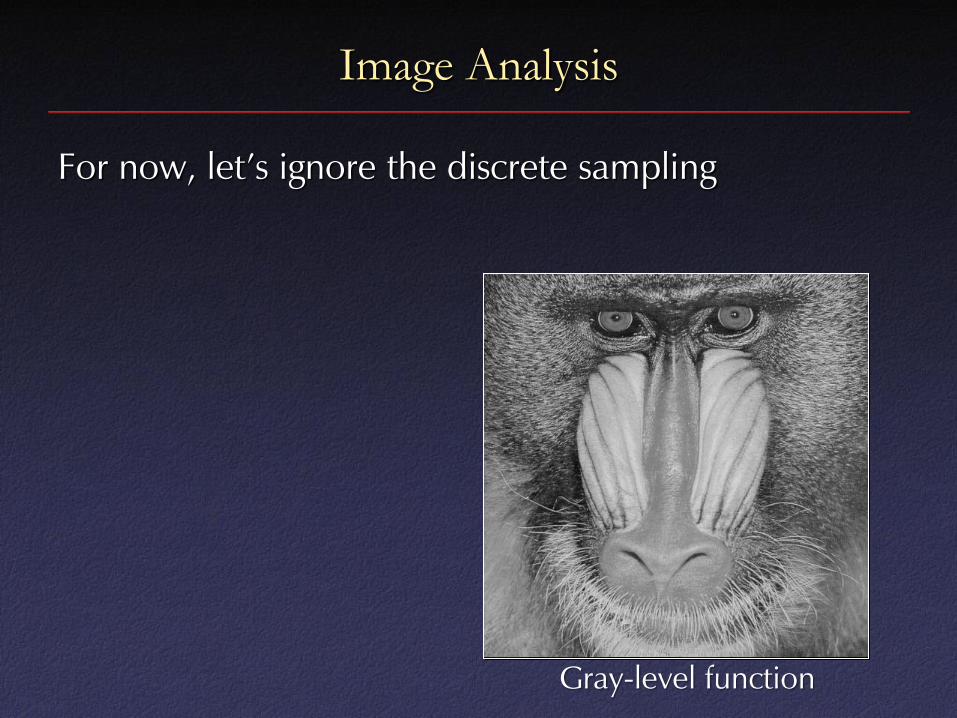
Image Analysis
For now, let’s ignore the discrete sampling
Gray-level function

Image Analysis
For now, let’s consider only one horizontal scanline
Gray-level function
x

Image Analysis
How do we analyze 1D continuous functions?

Image Analysis
How do we analyze 1D continuous functions?
• One useful tool is frequency analysis
|F(u)| f(x)
Spatial domain Frequency domain

Frequency Analysis
Any f(x) can be written as a sum of periodic functions
|F(u)|

Frequency Analysis
Fourier transform of function f is
F(u) is a function of frequency u describing how
much of each frequency f contains

Frequency Analysis
Fourier transform has real and imaginary parts:

Frequency Analysis
How does this work for 2D functions?

Frequency Analysis
The Fourier Transform is separable:

Frequency Analysis
Examples:
f(x,y) |F(u,v)|

Frequency Analysis
Examples:
f(x,y) |F(u,v)|

Frequency Analysis
Examples:
f(x,y) |F(u,v)|

Frequency Analysis
Examples:
f(x,y) |F(u,v)|

Frequency Analysis
Examples:
f(x,y) |F(u,v)|

Frequency Analysis
Examples:
f(x,y) |F(u,v)|

Frequency Analysis
Examples:
f(x,y) |F(u,v)|

Frequency Analysis
Examples: Gaussian
f(x,y) |F(u,v)|
2
22
222
2
1),(
yx
eyxG

Frequency Analysis
Examples:
f(x,y)
|F(u,v)|

Frequency Analysis
Examples:
f(x,y)
|F(u,v)|

Frequency Analysis
The Fourier transform has an inverse:

Application 1: Reducing Noise
f(x,y)
Zoomed
Noise is unwanted
(random) energy in
high frequencies
|F(u,v)|

Application 1: Reducing Noise
f(x,y)
|F(u,v)|
Original High frequencies removed

Application 1: Reducing Noise
Can reduce noise by convolving image with a
Gaussian filter
t
dttxgtfxgxf )()()()(

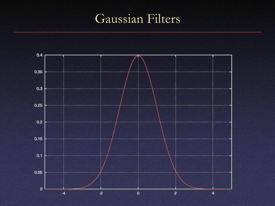
Gaussian Filters
What is a Gaussian filter?
• One-dimensional Gaussian
• Two-dimensional Gaussian
2
2
2
21
2
1)(
x
exG
2
22
222
2
1),(
yx
eyxG
Gaussian Filters

Gaussian Filters

Convolution
How do we convolve an image with a filter?
t
dttxgtfxgxf )()()()(
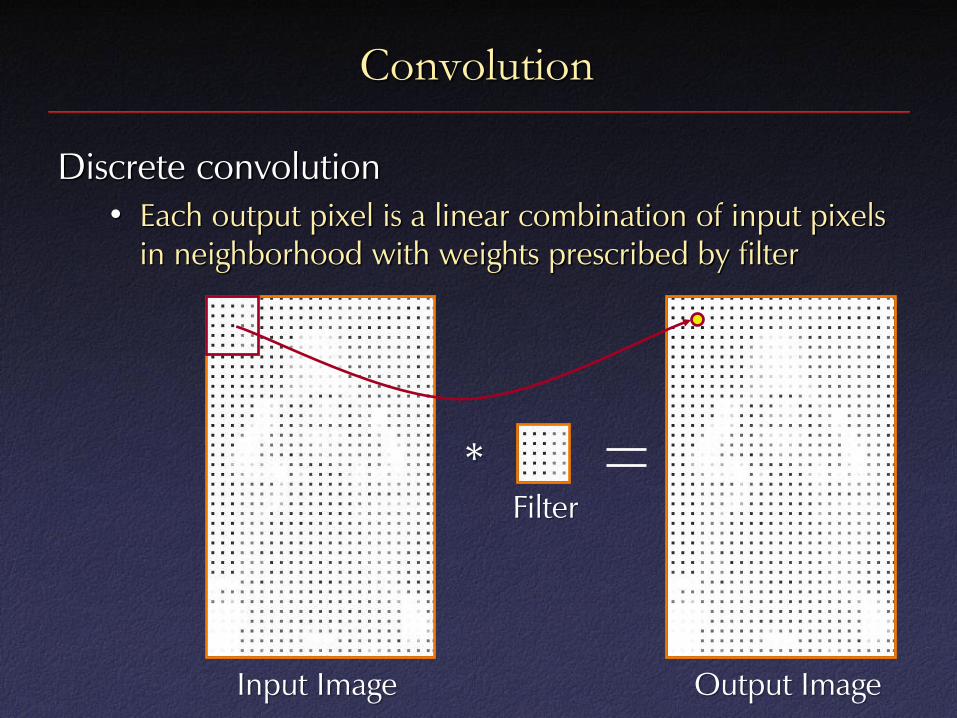
Convolution
Discrete convolution
• Each output pixel is a linear combination of input pixels
in neighborhood with weights prescribed by filter
Input Image Output Image
*
Filter
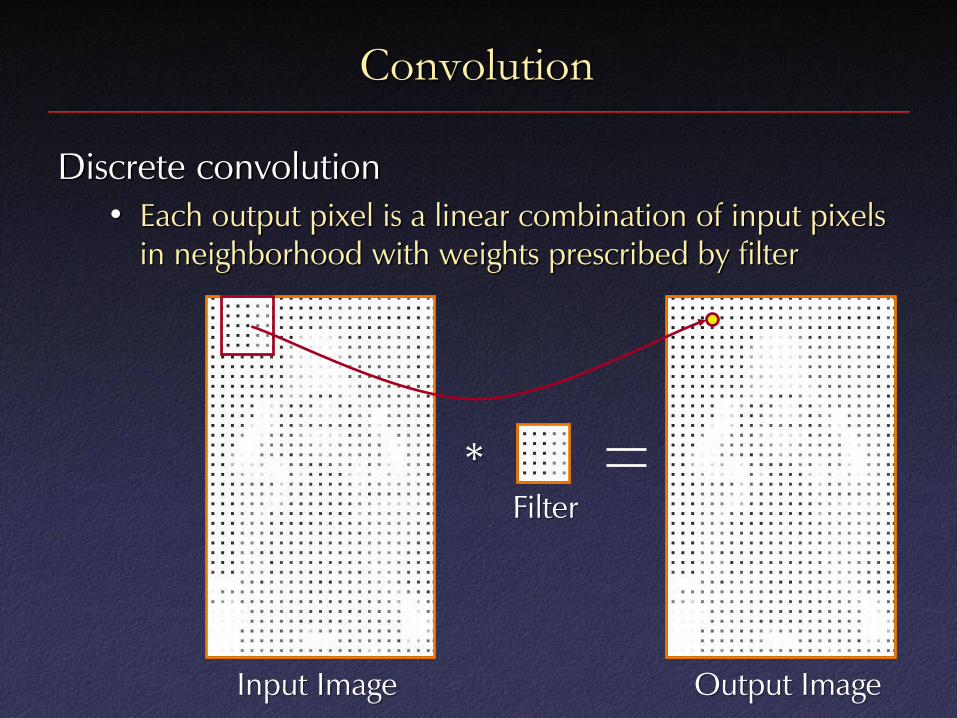
Convolution
Discrete convolution
• Each output pixel is a linear combination of input pixels
in neighborhood with weights prescribed by filter
Input Image Output Image
*
Filter

Convolution
Discrete convolution
• Each output pixel is a linear combination of input pixels
in neighborhood with weights prescribed by filter
Input Image Output Image
*
Filter

Convolution
Discrete convolution
• Each output pixel is a linear combination of input pixels
in neighborhood with weights prescribed by filter
Input Image Output Image
*
Filter

Convolution
Discrete convolution
• Naïve process takes O(n2m
2) … OK for small filters (m)
*
m
n
n

Fourier Transform and Convolution
Useful fact: multiplication in frequency domain is
same as convolution in spatial domain
f(x) * g(x) = F -1 ( F (f(x)) F (g(x)) )
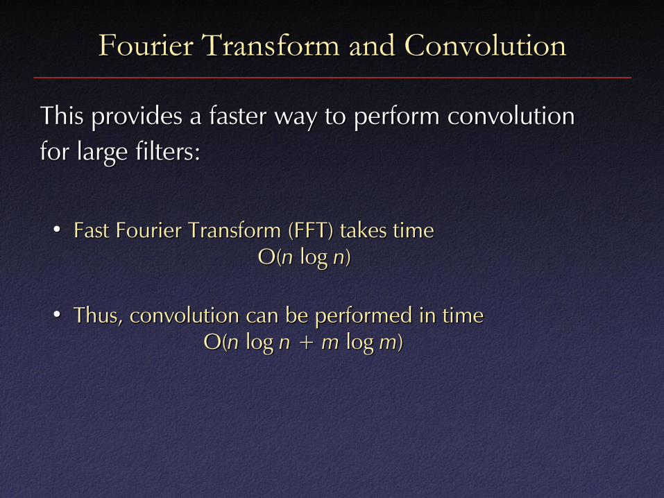
Fourier Transform and Convolution
This provides a faster way to perform convolution
for large filters:
• Fast Fourier Transform (FFT) takes time
O(n log n)
• Thus, convolution can be performed in time
O(n log n + m log m)

Fourier Transform and Convolution
Also, helps us reason about effects of specific filters
f(x,y)
|F(u,v)|
=
= x
*
Gaussian

Application 2: Reconstructing Frescoes

Application 2: Reconstructing Frescoes
Akrotiri = buried city discovered in 1967

Application 2: Reconstructing Frescoes
Many walls were decorated with wall paintings

Application 2: Reconstructing Frescoes
Many walls were decorated with wall paintings
Application 2: Reconstructing Frescoes
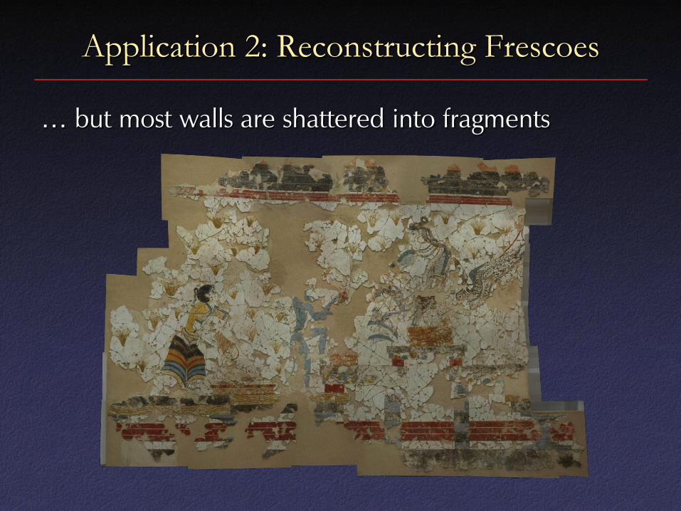
… but most walls are shattered into fragments

Application 2: Reconstructing Frescoes
… but most walls are shattered into fragments

Application 2: Reconstructing Frescoes
… and re-assembling the fragments is difficult

Application 2: Reconstructing Frescoes
… and re-assembling the fragments is difficult

Application 2: Reconstructing Frescoes
Our project: scan surfaces of fragments
Surface
image
Fracture
surface

Application 2: Reconstructing Frescoes
Our work: find matches between fragments

Application 2: Reconstructing Frescoes
Our work: reconstruct fresco from matches
Candidate fragment matches Reconstructed Fresco

Application 2: Reconstructing Frescoes
It turns out that subtle patterns in surface images
are good cues for finding matches
Surface patterns on a fresco fragment
(colors on right represent normal directions)
Toler-Franklin et al.

Application 2: Reconstructing Frescoes
Brush strokes appear as periodic functions with
dominant frequency and orientation
Brush patterns on different fresco fragments
(colors represent normal directions)
Toler-Franklin et al.

Application 2: Reconstructing Frescoes
Brush strokes appear as periodic functions with
dominant frequency and orientation
f(x) F(u) Dominant frequency
and direction
Toler-Franklin et al.

Application 2: Reconstructing Frescoes
Consider alignment of brush strokes and other surface
features when searching for matches
Toler-Franklin et al.

Image Analysis
What other tools do we have for analyzing functions?

Image Analysis
What other tools do we have for analyzing functions?
x
f(x)

Image Analysis
What other tools do we have for analyzing functions?
• Let’s look at gradients
x
f(x) f’(x)

Image Gradients
For 2D function f(x,y), the partial derivative is:
For discrete data, we can approximate using finite differences:
),(),(lim
),(
0
yxfyxf
x
yxf
1
),(),1(),( yxfyxf
x
yxf

Image Gradients
The gradient of an image:
The magnitude of the gradient:
The direction of the gradient:
y
yxf
),(

Computing Image Gradients
This is a convolution with two simple filters:
-1
1
1
-1 or
-1 1 x
yxf
),(
y
yxf
),(

Computing Image Gradients
Other common gradient filters:

Computing Image Gradients
We usually limit high frequencies when computing
gradient
x

Computing Image Gradients
We usually limit high frequencies when computing
gradient
x

Computing Image Gradients
Useful fact #1: differentiation
“commutes” with convolution
Useful fact #2: Gaussian is
separable:
dx
dgfgf
dx
dg
dx
df
)()(),( 112 yGxGyxG

Computing Image Gradients
Thus, combine smoothing with gradient computation:
)()(),(
)()(),(
)()(),(
)()(),(),(),(
11
11
11
11
2yGxGyxf
yGxGyxf
yGxGyxf
yGxGyxfyxGyxf

Computing Image Gradients
Can use different sigma to find gradients at different
“scales”
1 pixel 3 pixels 7 pixels

Gradient Analysis
How are image gradients useful?
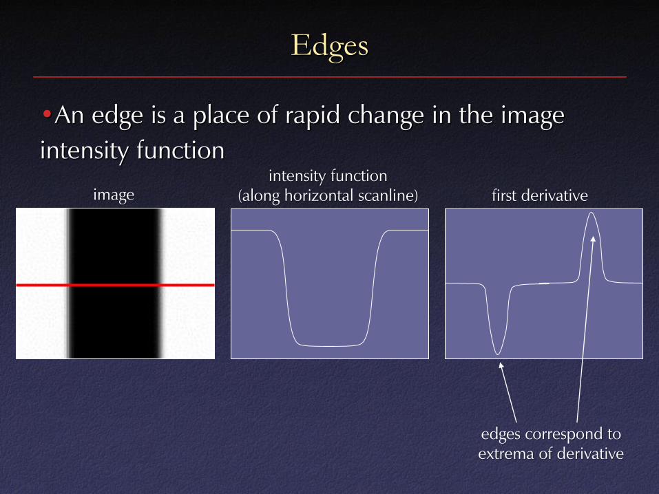
Edges
•An edge is a place of rapid change in the image
intensity function
image
intensity function
(along horizontal scanline) first derivative
edges correspond to
extrema of derivative

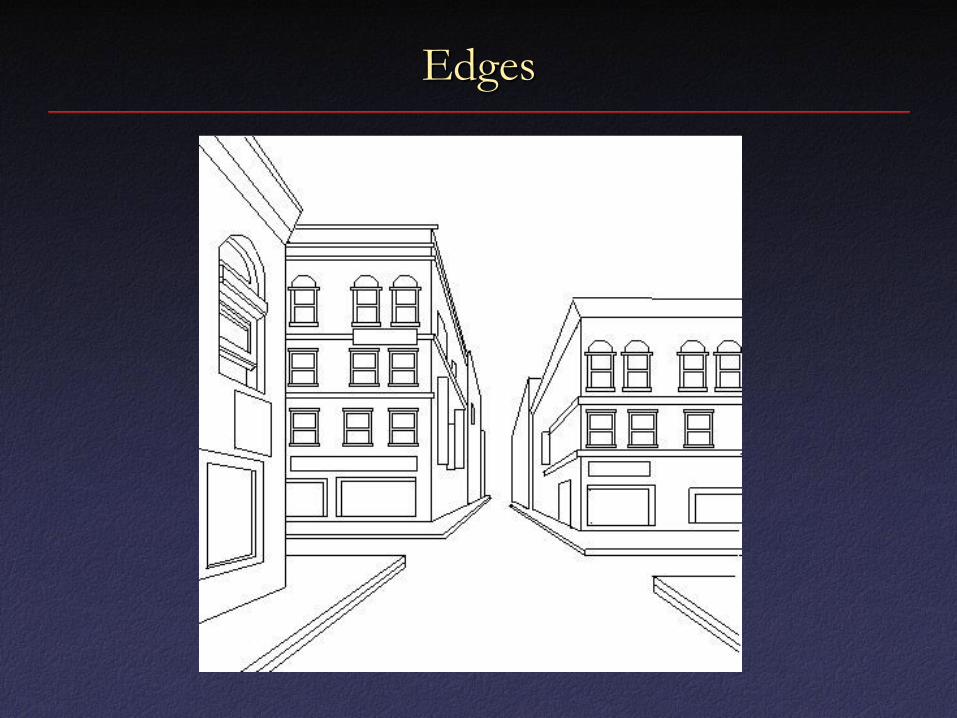
Edges
Silhouette
Boundary
Convex
Crease
Shadow
Boundary
Concave Crease


Edge Detection
Useful for many applications in vision
• Segmentation
• Camera pose estimation
• 3D reconstruction
• Object classification
• Object recognition
• etc.

Canny Edge Detector
1. Filter image with derivative of Gaussian
2. Find magnitude and orientation of gradient
3. Non-maximum suppression
4. Hysteresis thresholding

Canny Edge Detector
Original Image Smoothed Gradient Magnitude

Canny Edge Detector
Nonmaximum suppression
• Eliminate all but local maxima in gradient magnitude
(sqrt of sum of squares of x and y components)
• At each pixel p look along direction of gradient:
if either neighbor is bigger, set p to zero
• In practice, quantize direction to horizontal,
vertical, and two diagonals
• Result: “thinned edge image”

Canny Edge Detector
Smoothed gradient magnitude Non-maximum suppression

Canny Edge Detector
Final stage: thresholding
Simplest: use a single threshold
Better: use two thresholds
• Find chains of touching edge pixels, all
low
• Each chain must contain at least one pixel
high
• Helps eliminate dropouts in chains, without being too
susceptible to noise
• “Thresholding with hysteresis”

Canny Edge Detector
Non-maximum suppression Canny edges
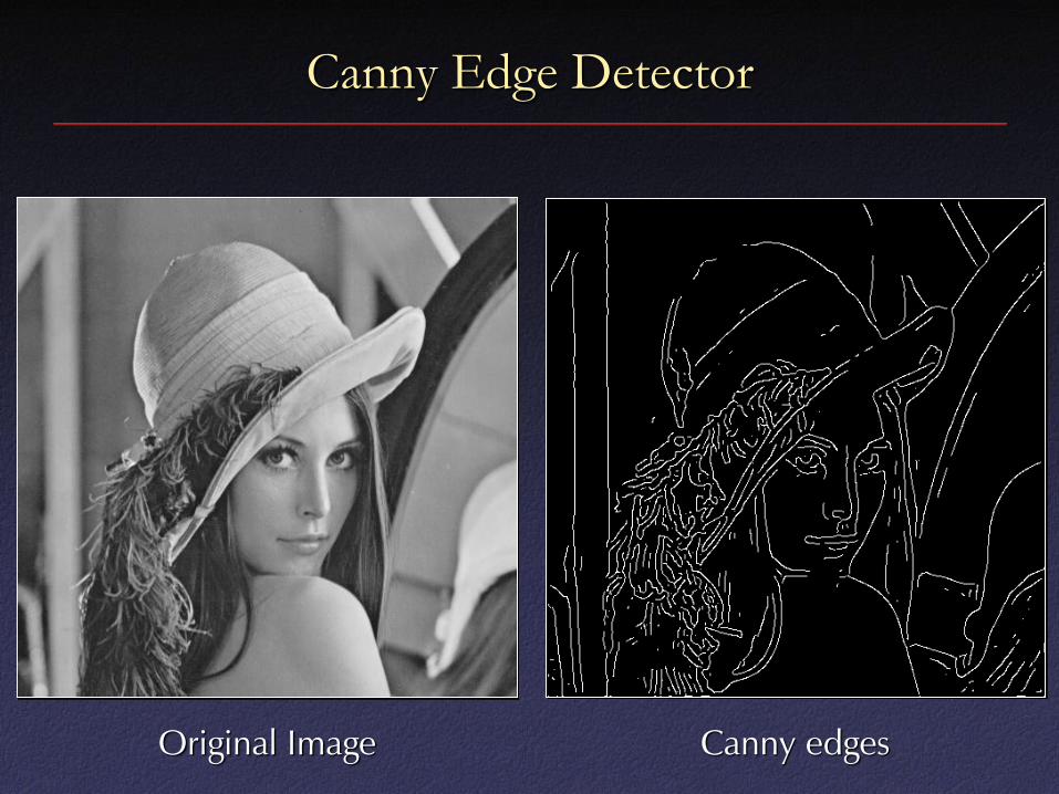
Canny Edge Detector
Original Image Canny edges

Summary of Canny Edge Detector
1. Filter image with derivative of Gaussian
2. Find magnitude and orientation of gradient
3. Non-maximum suppression:
• Thin wide “ridges” down to single pixel width
4. Hysteresis thresholding:
• Define two thresholds: low and high
• Use the high threshold to start edge curves and the low
threshold to continue them

Summary of Today
Image analysis:
• Frequency analysis
• Fourier transform
• Convolution
• Gradient analysis
• Edge detection