filtering historical simulation. backtest analysis · filtered historical simulation 1 filtering...

Filtered Historical Simulation

1

Filtering Historical Simulation. Backtest Analysis1

By Giovanni Barone-Adesi, Kostas Giannopoulos and Les Vosper

March 2000

A new generation of VaR models, based on historical simulation (boot-strapping), is being increasingly used in the risk management indus-try. It consists of generating scenarios, based on historical pricechanges, for all the variables in the portfolio. Since the estimatedVaR is based on the empirical distribution of asset returns it re-flects a more realistic picture of the portfolio’s risk. Unfortu-nately this methodology has a number of disadvantages. To overcomesome of them Barone-Adesi, Bourgoin and Giannopoulos(1998) and Bar-one-Adesi, Giannopoulos and Vosper (1999) introduce filtered histori-cal simulation (FHS hereafter). They take into account the changes inpast and current volatilities of historical returns and make theleast number of assumptions about the statistical properties of fu-ture price changes.

In this paper we backtest the FHS VaR model on three types of portfo-lios invested over a period of two years. The first set of backtestsconsists of LIFFE financial futures and options contracts traded onLIFFE. In the second set of backtests we examine the suitability ofthe FHS model on interest rate swaps. Finally, we backtest a set ofmixed portfolios consisting of LIFFE interest rate futures and op-tions as well as plain vanilla swaps.

We go beyond the strict criteria of the BIS recommendations by evalu-ating daily risk at four different confidence levels and five differ-ent trading horizons for a large number of realistic portfolios2 ofderivative securities.

In the first section we describe the backtesting methodology and re-port the results for the LIFFE portfolios. To enable us to appraisethe different components of risk measurements on each of the threetypes of portfolios we run three sets of backtests, relaxing the fol-lowing assumptions in each test: in the first backtest we keep con-stant implied volatilities and FX rates. Our analysis focuses on howwell FHS predicts losses due to futures and options market pricechanges. In our second backtest we simulate implied volatilitieswhile in the third backtest we also take into account the portfolios’FX exposure. Our results show that fixed implied volatility performsbetter at short VaR horizons, while at longer ones (5 to 10 days) ourstochastic implied volatility performs better.

1 Universita’ della Svizzera Italiana and City University Business School, Westminster BusinessSchool and London Clearing House. We are grateful to The London Clearing House for providing usthe data and financing the project.2 For backtest 1, a total of 75,835 daily portfolios; backtests 2 and 3 have a total of 75,985 portfolios.


2

In the second series of backtests we investigate the performance ofFHS on books of interest rate swaps. We compare each book’s dailyvalues with the FHS lower forecasted value. For each book we producetwo types of forecast; an aggregate market value risk expressed inGBP and a set of currency components (plain vanilla swaps in USD,JPY, DEM, and GBP are used). In the swap portfolios we find that ourmethodology is too conservative at longer horizons.

In the final set of backtests we investigate the performance of theFHS model on diversified portfolios across plain vanilla swaps andfutures and options traded on LIFFE. This study shares the same datawith the separate LIFFE and Swaps backtests but restricts the numberof portfolios to 20 among the largest members on LIFFE. By adding toeach LIFFE portfolio one of the four swap books3 used in the swapsbacktest we form 20 combined (combo) portfolios.

Our analysis is based on two criteria: statistical and economic. Theformer examine the frequency and the pattern of losses exceeding theVaR predicted by FHS (breaks); the latter examine the implications ofthese breaks in economic terms, with reference to the total VaR allo-cated. Overall our findings sustain the validity of FHS as a riskmeasurement model. Furthermore, we find that diversification reducesrisk effectively across the markets we study.

3 Four SWAP books consisting of 500 Swaps each were formed for the SWAP backtest. Details of theportfolios are available from the authors.


3

1 Overview of VaR models.

VaR models play a core role in the risk management of today’s financial institutions. A number ofVaR models are in use. All of them have the same aim, to measure the size of possible future losses ata predetermined probability. There are a variety of approaches used by VaR models to estimate thepotential losses. Models differ in fact in the way they calculate the density function of future profitsand losses of current positions, as well as the assumptions they rely on. Although VaR analysis hasbeen used since early 1980’s by some departments of few large financial institutions it wasn’t until themiddle 1990’s that it became widely accepted by banks and also imposed by the regulators. The cor-nerstone behind this wide acceptance was a linear VaR model, based on the variance-covariance ofpast security returns, introduced by JP Morgan, RiskMetrics (1993). The variance-covariance ap-proach to calculate risk can be traced back to the early days of Markowitz’s (1959) Modern PortfolioTheory, which is now common knowledge among today’s risk managers.

Linear VaR models, however, impose strong assumptions about the underlying data. For example, thedensity function of daily returns follows a theoretical distribution (usually normal) and has constantmean and variance4. The empirical evidence about the distributional properties of speculative pricechanges provides evidence against these assumptions5, e.g. Kendall (1953) and Mandelbrot (1963).Risk managers have also seen their daily portfolio’s profits and losses to be much larger than thosepredicted by the normal distribution. The RiskMetrics VaR method has two additional major limita-tions. It linearises derivative positions and it does not take into account expiring contracts. Theseshortcomings may result in large biases, particularly for longer VaR horizons and for portfoliosweighed with short out-of-the money options.

To overcome problems of linearising derivative positions and to account for expiring contracts, riskmanagers have begun to look at simulation techniques. Pathways are simulated for scenarios for lin-ear positions, interest rate factors and currency exchange rate and are then used to value all positionsfor each scenario. The VaR is estimated from the distribution (e.g. 1st percentile) of the simulatedportfolio values. Monte-Carlo simulation is widely used by financial institutions around the globe.Nevertheless, this method can attract severe criticisms. First, the generation of the scenarios is basedon random numbers drawn from a theoretical distribution, often normal, which not only does notconform to the empirical distribution of most asset returns, but also limits the losses to around three orfour standard deviations when a very large number of simulation runs is carried out. Second, tomaintain the multivariate properties of the risk factors when generating scenarios, historical correla-tions are used; during market crises, when most correlations tend to increase rapidly, a Monte Carlosystem is likely to underestimate the possible losses. Third, historical simulation tends to be slow, be-cause a large number of scenarios which has to be generated6.

Barone-Adesi and Giannopoulos (1996) argue that the covariances (and correlations) are unnecessaryin calculating portfolio risk7. They suggested the creation of a synthetic security by multiplying cur-rent portfolio weights by the historical returns of all assets in the portfolio. They fit a conditionalvolatility model on these historical returns to estimate the last trading day’s volatility and then calcu-late the portfolio’s VaR as in RiskMetrics (1993). Barone-Adesi, Bourgoin and Giannopoulos (1988)

4 The RiskMetrics VaR approach recognises the fact that variances and covariances are changingover time and use a simple method (exponential smoothing) to capture these changes. They contradictthemselves, however, and use a constant volatility assumption for the multi-period VaR (i.e. the lasttrading day’s volatility is scaled with the time).5 However the extent to which these assumptions are violated depend on the frequency of the data.Daily data, which are of interest in risk management, tend to deviate to a great extend from normality.6 Jamshidian and Zhu (1997) proposed a method that limits the number of portfolio valuations.7 Markowitz introduced the variance-covariance matrix in his portfolio risk approach but had a differ-ent objective to risk managers. Markowitz aim was to find optimal risk/return portfolio weights ratherthan trying to measure risks of a (known) portfolio.


4

have suggested to draw random standardised returns8 from the portfolio’s historical sample and afterrescaling these standardasied historical returns with the current volatility, to use them as innovationsin a conditional variance equation for generating scenarios for both future portfolio variance and price(level)9. This method not only generates scenarios that conform with to the past history of the currentportfolio’s profits and losses, but also overcomes an additional limitation of the variance-covariancemodel. It allows both past and future volatility to vary over time. The creation of a synthetic securitysimplifies the computational effort to a large extent. However, it suffers from the above criticismswhen handling non-linear positions (it uses the options delta to linearise them).

Recognising the fact that most asset returns cannot be described by a theoretical distribution, an in-creasing number of financial institutions are using historical simulation. Here, each historical obser-vation forms a possible scenario, see Butler and Schachter (1998). A number of scenarios is generatedand in each of them all current positions are priced. The resulting portfolio distribution is more real-istic since it is based on the empirical distribution of risk factors. This method has still some seriousdrawbacks. Historical simulation ignores the fact that asset risks are changing all the time. The his-torical returns that are used as if they are random numbers are not i.i.d., and so, are unsuitable for anysimulation. Thus the VaR value will be biased. During high volatile market conditions the historicalsimulation will underestimate risk. Furthermore, historical simulation uses constant implied volatilityto price the options under each scenario. Some positions which may be appear well-hedged under theconstant implied volatility hypothesis, may become very risky under a more realistic scenario. It wouldbe difficult to determine the extent of this problem as sensitivity analysis is difficult with historicalsimulation.

1.1 Filtered historical Simulation

To overcome the shortcomings of historical simulation it is necessary to filter historical returns; thatis to adjust them to reflect current information about security risk. Our complete filtering methodologyis discussed in Barone-Adesi, Giannopoulos and Vosper (1999). A brief synopsis is presented below.

1.1.11.1.1 Simulating a Single PathwaySimulating a Single Pathway

Many pathways of prices are simulated for each contract (asset or interest rate) in our dataset overseveral holding periods. In our backtests we use 5000 simulations results over 10 days. The algo-rithm is described by starting with the simulation of a single pathway out of the 5000, for a singlecontract. From this we can generalise to the simulation of many pathways for many contracts, andtheir aggregation into portfolio pathways. The set of portfolio pathways for each day in the holdingperiod defines 10 empirical distributions i.e. over holding periods from 1 to 10 days.

Our methodology is non-parametric in the sense that simulations do not rely on any theoretical distri-bution on the data as we start from the historical distribution of the return series. We use two years ofearlier data to calibrate our GARCH models, (Bollerslev 1986), for asset returns and to build the databases necessary to our simulation. By calibrating GARCH models to the historical data we form resid-ual returns from the returns series. Residual returns are then filtered to become identically and inde-pendently distributed, removing serial correlation and volatility clusters. As the computation of thei.i.d. residual returns involves the calibration of the appropriate GARCH model,10 the overall ap-proach can be described as semi-parametric. For example, assuming a GARCH(1,1) process with both

8 The portfolio’s standardised returns must be i.i.d. If this is not the case then a mean equation thatyields i.i.d. residuals is fitted.9 See section 1.1.110 For example one asset may use GARCH (1,1) with no AR or MA terms, another may employAGARCH with an MA term; we examine a variety of processes to attempt to fit the appropriate modelto the data series of each asset.


5

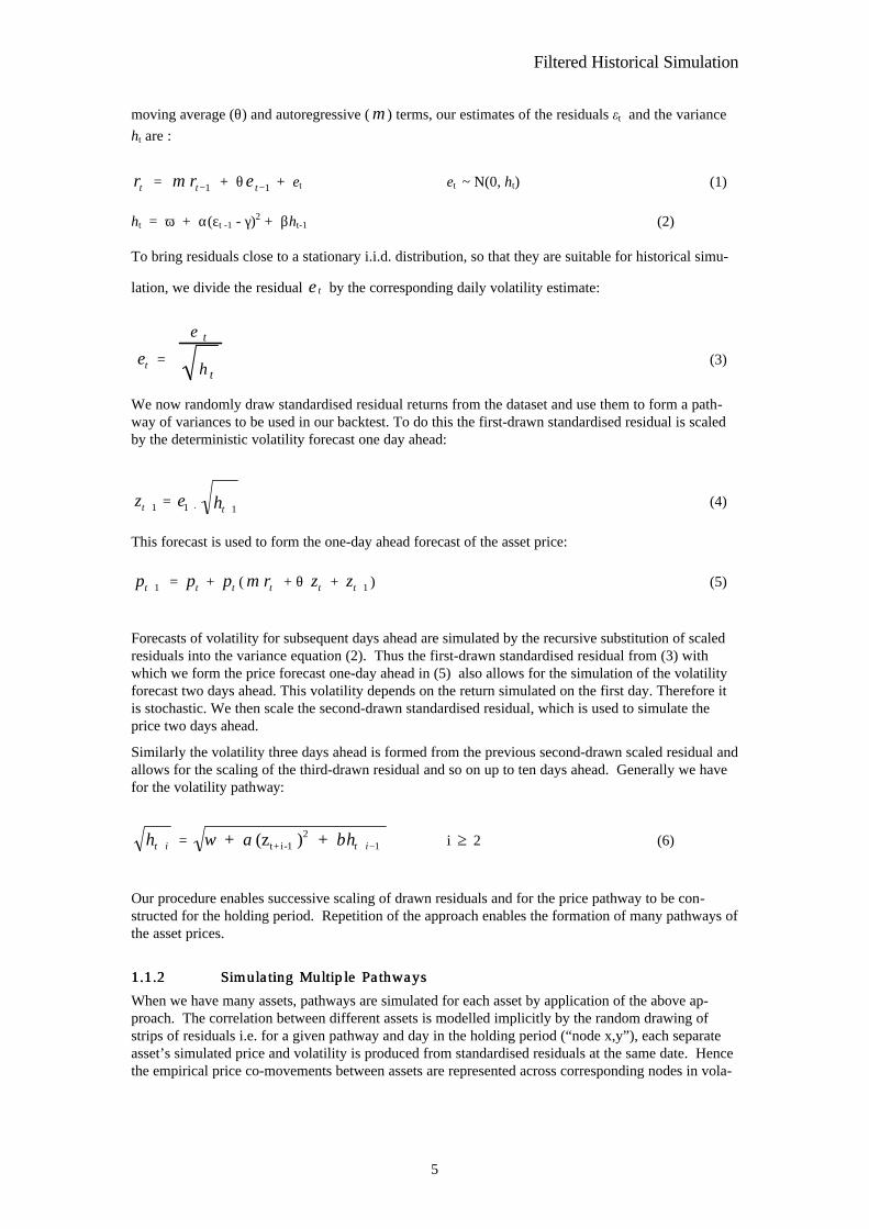
moving average (θ) and autoregressive ( µ ) terms, our estimates of the residuals et and the variance

ht are :

rt = µ rt −1 + θ ε t −1 + εt εt ~ N(0, ht) (1)

ht = ω + α(εt -1 - γ)2 + βht-1 (2)

To bring residuals close to a stationary i.i.d. distribution, so that they are suitable for historical simu-

lation, we divide the residual ε t by the corresponding daily volatility estimate:

et =

ε t

th(3)

We now randomly draw standardised residual returns from the dataset and use them to form a path-way of variances to be used in our backtest. To do this the first-drawn standardised residual is scaledby the deterministic volatility forecast one day ahead:

zt +1 = e1 . ht +1(4)

This forecast is used to form the one-day ahead forecast of the asset price:

pt +1 = pt + pt ( µ rt + θ zt + zt +1 ) (5)

Forecasts of volatility for subsequent days ahead are simulated by the recursive substitution of scaledresiduals into the variance equation (2). Thus the first-drawn standardised residual from (3) withwhich we form the price forecast one-day ahead in (5) also allows for the simulation of the volatilityforecast two days ahead. This volatility depends on the return simulated on the first day. Therefore itis stochastic. We then scale the second-drawn standardised residual, which is used to simulate theprice two days ahead.

Similarly the volatility three days ahead is formed from the previous second-drawn scaled residual andallows for the scaling of the third-drawn residual and so on up to ten days ahead. Generally we havefor the volatility pathway:

ht i+ = ω α β + (z ) + t+ i-12 ht i+ −1 i ≥ 2 (6)

Our procedure enables successive scaling of drawn residuals and for the price pathway to be con-structed for the holding period. Repetition of the approach enables the formation of many pathways ofthe asset prices.

1.1.21.1.2 Simulating Multiple PathwaysSimulating Multiple Pathways

When we have many assets, pathways are simulated for each asset by application of the above ap-proach. The correlation between different assets is modelled implicitly by the random drawing ofstrips of residuals i.e. for a given pathway and day in the holding period (“node x,y”), each separateasset’s simulated price and volatility is produced from standardised residuals at the same date. Hencethe empirical price co-movements between assets are represented across corresponding nodes in vola-


6

tility and price pathways11. The price pathways for assets in a portfolio can therefore be aggregated, toproduce portfolio price distributions, without resorting to the correlation matrix, or assuming any par-ticular distribution for the data. The procedure is non-parametric apart from assumptions used in theestimation of residuals in the GARCH process (see equation 1).12

For assets in different currencies, the methodology can produce pathways of simulated currency ex-change rates, so that all values are expressed in a common currency. The historical residuals derivedfrom changes in exchange rates are included in the dataset so that they are a part of the random re-siduals strips used during simulation, so that FX moves are produced simultaneously with asset (orinterest rate) moves.

In this way, assets’ pathways, FX pathways and interest rate pathways13 are constructed from histori-cal returns modified through GARCH filters. We go beyond historical simulation by scaling the ran-dom set of returns to produce i.i.d. standardised residuals; these standardised residuals are then scaledagain to reflect current and forecast volatilities14. For certain scenarios, the successive prices in apathway will have been constructed from one large return following another, so that extreme scenariosare generated, beyond those generally used in Value at Risk estimations.

If a portfolio contains non-linear derivatives e.g. options, their pathways are produced by using theappropriate options model with the pathways of underlying assets as inputs. Implied volatility caneither be assumed to be constant over the holding period, or pathways of implied volatilities can beproduced that relate to the simulated variance pathways given suitable assumptions. In our back-testing, we consider both possibilities.

Section 1: Backtesting interest rate futuresand options

This section describes the first set of backtests, applied to LIFFE member portfolios. For each tradingdate over a period of nearly 2 years (4 January 1996 to 12 November 1997), we use the filtered his-torical simulation (therefore FHS) to measure the market risk on LCH members with positions inLIFFE financial products. We compare the daily profits and losses for each portfolio with FHS-generated risk measures. We use only information available at the end of each trading date (positionsand closing prices) to measure the market risk of each portfolio for horizons of up to 10 working days.Consequently, we compare the actual trading results of these portfolios15 with the risk values predictedby FHS. This process is known as “backtesting”, it is recommended by the Basle Committee (1996)and has been adopted by many financial institutions to gauge the quality and accuracy of their riskmeasurement models.

2 The Backtesting processFor each business day from 4 January 1996 until 12 November 1997 we use the FHS methodology tocalculate the market risk of all LIFFE members with positions in interest rate contracts (German

11 For a detailed description of the algorithm see Barone-Adesi, Giannopoulos and Vosper (1999).12 GARCH constants have been maximum likelihood-estimated by assuming residuals in (1) are nor-mally distributed.13 These constitute points on zero coupon curves allowing us to produce simulations of entire curves,with co-movements implicitly linked to all other prices and rates.14 Volatilities themselves are simulated over the holding period for each scenario or pathway.15 Portfolio weights i.e. net positions, are kept constant for 1 to ten days.


7

Bund, BTP, Long Gilt, Short Sterling, Euromark, 3 month Swiss, Eurolira respectively). In this sec-tion we run three sets of backtests. During the first we keep constant the FX and the implied volatility(i.e. neither is allowed to change during the VaR horizon). In the second set the implied volatility oneach option is modelled as a function of the stochastic volatility of the underlying asset; this enablesthe generation of more realistic scenarios to be generated. In the final set, we generate pathways forFX-to-sterling rate. This enables us to incorporate the FX risk of the pathways of futures and optionsprices. In most VaR systems FX risk increases the complexity of a VaR system by a large factor. Inour case, however, there is no additional computational complexity; the size of the problem increaseslinearly with the number of currencies in the portfolio.

In each of our three backtests we stored the risk measures of five different VaR horizons (1, 2, 3, 5and 10 days) and four different probability levels (0.95, 0.98, 0.99 and 0.995). We estimate daily riskmeasures for about 158 portfolios for a period of 480 days. These values are subsequently comparedto the actual ones and the number of breaks is recorded.

2.1 Calculation of Value Losses

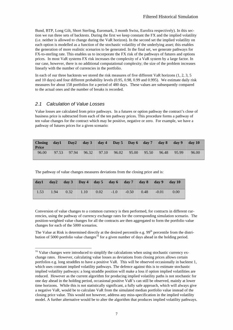
Value losses are calculated from price pathways. In a futures or option pathway the contract’s close ofbusiness price is subtracted from each of the ten pathway prices. This procedure forms a pathway often value changes for the contract which may be positive, negative or zero. For example, we have apathway of futures prices for a given scenario:

ClosingPrice

day1 Day2 day 3 day 4 Day 5 Day 6 day 7 day 8 day 9 day 10

96.00 97.53 97.94 96.32 97.10 96.02 95.00 95.50 96.48 95.99 96.00

The pathway of value changes measures deviations from the closing price and is:

day1 day2 day 3 Day 4 day 5 day 6 day 7 day 8 day 9 day 10

1.53 1.94 0.32 1.10 0.02 -1.0 -0.50 0.48 -0.01 0.00

Conversion of value changes to a common currency is then performed, for contracts in different cur-rencies, using the pathway of currency exchange rates for the corresponding simulation scenario. Theposition-weighted value changes for all the contracts are then aggregated to form the portfolio valuechanges for each of the 5000 scenarios.

The Value at Risk is determined directly at the desired percentile e.g. 99th percentile from the distri-bution of 5000 portfolio value changes16 for a given number of days ahead in the holding period.

16 Value changes were introduced to simplify the calculations when using stochastic currency ex-change rates. However, calculating value losses as deviations from closing prices allows certainportfolios e.g. long straddles to have a positive VaR. This will be observed occasionally in backtest 1,which uses constant implied volatility pathways. The defence against this is to estimate stochasticimplied volatility pathways: a long straddle position will make a loss if option implied volatilities arereduced. However as the current algorithm for producing implied volatility paths is not stochastic forone day ahead in the holding period, occasional positive VaR’s can still be observed, mainly at lowertime horizons. While this is not statistically significant, a fully safe approach, which will always givea negative VaR, would be to calculate VaR from the simulated median portfolio value instead of theclosing price value. This would not however, address any miss-specification in the implied volatilitymodel. A further alternative would be to alter the algorithm that produces implied volatility pathways.


8

2.2 Calculation of Breaks

2.2.12.2.1 Re-marking Portfolios to MarketRe-marking Portfolios to Market

For a given close of business date, portfolios are re-marked to market for each of the subsequent tendays, to correspond to the days ahead in the holding period. This is done in an analogous fashion toforming value losses in FHS: for the first day ahead in the holding period, the actual closing price forthis date has the closing price at the close of business subtracted from it. This is repeated for each ofthe dates corresponding to the holding period i.e. the close of business price is subtracted from theclosing prices on these dates.

The actual portfolio gain or loss from closing price values is therefore computed in the same way thatFHS calculates portfolio value changes, using the actual corresponding currency exchange rates.

2.2.22.2.2 The BreaksThe Breaks

As VaR’s and portfolio actual gains or losses are calculated consistently, they can be compared di-rectly to each other, for the corresponding number of days ahead in the holding period. The objectivein FHS is to exceed the actual portfolio losses a certain percentage of the time corresponding to theconfidence level used. This means that some of the time the VaR will not be sufficient to cover anactual loss. For example for 99% confidence, “breaks” should occur 1% of the time.

To compute whether a break has occurred:

If (VaR > change in actual portfolio value) then a break has occurred.17

2.2.32.2.3 Expiring PositionsExpiring Positions

(i) Positions in delivery (i.e. the contract has ceased trading before the current close of business) areout of scope and are not included in portfolios.

(ii) Futures and options contracts that expire on the close of business18 are not included in the portfo-lio (i.e. contracts with positions having zero days to expiry).

(iii) Futures and options contracts that expire the next day are not included in the portfolio (i.e. con-tracts with positions having one day to expiry).

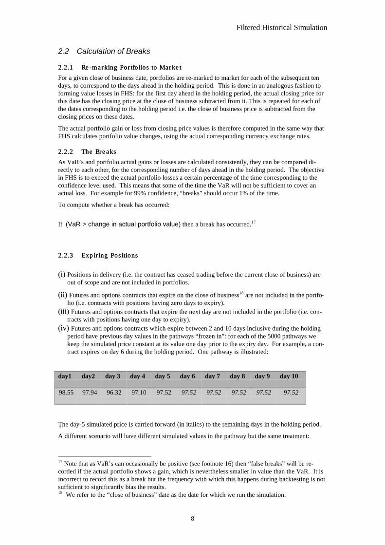
(iv) Futures and options contracts which expire between 2 and 10 days inclusive during the holdingperiod have previous day values in the pathways “frozen in”: for each of the 5000 pathways wekeep the simulated price constant at its value one day prior to the expiry day. For example, a con-tract expires on day 6 during the holding period. One pathway is illustrated:

day1 day2 day 3 day 4 day 5 day 6 day 7 day 8 day 9 day 10

98.55 97.94 96.32 97.10 97.52 97.52 97.52 97.52 97.52 97.52

The day-5 simulated price is carried forward (in italics) to the remaining days in the holding period.

A different scenario will have different simulated values in the pathway but the same treatment:

17 Note that as VaR’s can occasionally be positive (see footnote 16) then “false breaks” will be re-corded if the actual portfolio shows a gain, which is nevertheless smaller in value than the VaR. It isincorrect to record this as a break but the frequency with which this happens during backtesting is notsufficient to significantly bias the results.18 We refer to the “close of business” date as the date for which we run the simulation.


9

day1 day2 day 3 day 4 day 5 day 6 day 7 day 8 day 9 day 10

99.52 98.44 97.99 97.65 96.48 96.48 96.48 96.48 96.48 96.48

2.3 Actual Portfolios

Actual portfolio values are calculated to reflect the above treatment i.e. a contract’s actual closingprice one day prior to its expiry date is “copied forward” to the expiry date and subsequent dates cor-responding to the holding period. This is done to ensure that re-marking to the market is consistentwith FHS.

3 Backtest I, part A (Constant FX & Implied Volatility)

During part A of the first backtest we hold implied volatility constant. Furthermore, to isolate the cur-rency risk from market value risk we translate all returns to sterling at the close of business FX rates.Here are the summary results:

3.1 Overall frequency tests

In Table 1, we show the Number of breaks across all portfolios for the 2-year period (total of 75,835daily portfolios). The number of breaks19 recorded across all portfolios for the entire backtest periodare reported in each column (D1, D2, D3, D5, and D10). D1, ... D10 are the 1, 2, 3, 5 and 10-dayVaR horizons. We record the breaks at each of the four confidence levels (percentiles) used in thebacktest. Below each number of breaks we report the corresponding percentage on the number of pre-dictions. The expected number of those percentage breaks should be equal to one minus the corre-sponding confidence interval.

The percentages of breaks are within 0.5% of the expected ranges, except at high confidence levelsand short horizons. However, some portfolios are more likely to report breaks than others are. Weidentified three such portfolios, “A”, “B” and “C”. Table 2 reports the aggregate number of breaks onthe three portfolios. Below the number of breaks is the percentage of breaks on the number of daysthese portfolios have traded during the 2-year period. In the line below we show the percentage of the

19 A break occurs when the portfolio trading loss is greater to the one predicted by BAGV for thatVaR horizon.

Table 1 Breaks across All Portfoliosc.i. D1 D2 D3 D5 D10

95% 3583 3701 3864 3580 34384.725% 4.880% 5.095% 4.721% 4.534%

98% 1906 1914 1846 1560 13902.513% 2.524% 2.434% 2.057% 1.833%

99% 1296 1194 1093 927 7461.709% 1.574% 1.441% 1.222% 0.984%

99.5% 938 810 711 561 4331.237% 1.068% 0.938% 0.740% 0.571%


10

breaks of these three portfolios on the overall number of breaks. As we can see, the three portfoliosaccount for up to 21.5% on the overall number of breaks20.

Table 3 reports the same statistics as Table 1 excluding the above three portfolios. To gauge the sta-tistical significance of these results, under the hypothesis of independence the above percentages aredistributed normally around their expected values, with standard deviations ranging from 0.2% (at95% level) to 0.06% (at 99.5% level). A two-standard deviation interval may be heuristically doubledto account for the dependence across portfolios, leading to a tolerance of 4 standard deviations. As wecan see when the three portfolios are excluded the backtest results marked with an asterisk still showsome significant differences from our success criteria.

3.2 Individual Firm Tests

These tests determine whether breaks occur randomly in our sample or cluster for some firms forwhich risk may be miss-specified. Under the null hypothesis of randomness the number of breaks inthe two halves of our backtesting period are independent. Therefore a cross-sectional regression of thebreaks, which each firm reports in the first half on the number of breaks reported in the second half,should have zero slope. The regression analysis on the breaks for each sub-period shows a bias at eachVaR horizon and each confidence level. However, when the three portfolios mentioned above are ex-cluded from the sample there is no significant correlation between the breaks reported in two sub-periods. Therefore the evidence of miss-specification is limited to those three anomalous portfolios.Table 4 reports some typical results (the significant slope is denoted by asterisk). The values in brack-ets are the standard errors.

20 i.e. on 1 day VaR at 99.5% probability.

Table 2 Cumulative Break Analysis for Portfolios A, B, and Cc.i. D1 D2 D3 D5 D10

95% 316 256 225 188 12322.316% 18.079% 15.890% 13.277% 8.686%8.819% 6.917% 5.823% 5.251% 3.578%

98% 256 197 175 139 7418.079% 13.912% 12.359% 9.816% 5.226%13.431% 10.293% 9.480% 8.910% 5.324%

99% 225 175 132 112 6015.890% 12.359% 9.322% 7.910% 4.237%17.361% 14.657% 12.077% 12.082% 8.043%

99.5% 201 146 119 91 4614.195% 10.311% 8.404% 6.427% 3.249%21.429% 18.025% 16.737% 16.221% 10.624%

Table 3 All portfolios except A, B and Cc.i. D1 D2 D3 D5 D10

95% 3267 3445 3639 3392 3315*4.390% 4.629% 4.890% *4.558% *4.455%

98% 1650 1717 1671 1421 1316*2.217% *2.307% *2.245% 1.909% *1.768%

99% 1071 1019 961 815 686*1.439% *1.369% *1.291% 1.095% 0.922%

99.5% 737 664 592 470 387*0.990% *0.892% *0.795% 0.632% 0.520%


11

3.3 Time clustering effect

Clustering tests assess whether days with large number of breaks across all the firms tend to be fol-lowed by other days with large numbers of breaks, pointing to a miss-specification of the time-seriesmodel of volatility. The evidence of that can be detected by autocorrelations in the aggregate numberof breaks occurring each day. We applied the Ljung-Box (1978) test and we found no evidence of sig-nificant serial correlation’s21 (order 1 to 6) for any confidence level at the 1-day VaR horizon. Theoverlapping of measurement intervals makes this test not applicable at longer horizons, because port-folios cannot then be regarded as being independent.

3.4 Economic Criteria

Breaks are more uniformly distributed when longer time horizons (5 or 10 days) are used. At shorterhorizons breaks cluster more (31 Dec 96, 28 Nov 96 and 7 March 96 are the days with the largestconcentrations of breaks). The worst day is 31 Dec 96, with 46 breaks adding up to £139M on a VaRof £285M (at 95% level and 1 day horizon). The sum of breaks in the worst day decreases slightlywhen the horizon increases to 10 days, but it decreases dramatically when the confidence level in-creases (it drops to 40% of the above figures, down to £42 M at 99.5% level and 10 days).

The sum of VaR’s (in Sterling) over the different days for all portfolios ranges within the followingintervals:

- 300M to 600M at 95% level and 1 day horizon- 750M to 1,800 M at 95% level and 10 day horizon- 400M to 1,000 M at 99.5% level and 1 day horizon- 1,200M to 3,000M at 99.5% level and 10 day horizon The ratio of total breaks on the worst day over total VaR ranges from 48% to 2%, depending on thechosen horizon and confidence level. It should be recalled that breaks are computed by not allowingany portfolio change or accounting for cash settlement to market over the VaR horizon. Our aggre-gate statistics beyond the number of breaks are not significantly affected by the three portfolios identi-fied above, because the sizes of their VaR and their breaks are minuscule (always less than £40,000,mostly close to zero).

21 Under the null hypothesis of zero correlation our test statistic is a chi-square with six degrees offreedom. At the 95% level, the critical value for the Chi-square test is 12.6.

Table 4 (3 Day VaR horizon at 99%)All portfolios Excluding three anomalous portfolios

a b a b0.271 0.599* 1.869 0.029

(0.442) (0.080) (0.389) (0.097)

Table 5 serial correlation test on 1 day VaRQ1 Q2 Q3 Q4 Q5 Q6

95% 0.03 0.68 2.61 3.29 5.18 5.1898% 0.92 1.51 1.72 1.78 1.89 2.5999% 0.02 0.8 0.81 0.87 0.92 1.17

99.50% 0.04 1 1 1.06 1.06 1.17


12

Figure 1 Sum of ten largest breaks on 10-Day VaR at 99%

Figure 2 VaR across all portfolios for a 10-day horizon at 99%

0

10,000,000

20,000,000

30,000,000

40,000,000

50,000,000

60,000,000

02-J

an-9

6

05-F

eb-9

6

08-M

ar-9

6

15-A

pr-9

6

20-M

ay-9

6

24-J

un-9

6

26-J

ul-9

6

30-A

ug-9

6

03-O

ct-9

6

06-N

ov-9

6

10-D

ec-9

6

16-J

an-9

7

19-F

eb-9

7

25-M

ar-9

7

30-A

pr-9

7

05-J

un-9

7

09-J

ul-9

7

12-A

ug-9

7

16-S

ep-9

7

20-O

ct-9

7

date

loss

es

0

500,000,000

1,000,000,000

1,500,000,000

2,000,000,000

2,500,000,000

3,000,000,000

01/0

2/96

02/0

1/96

03/0

4/96

04/0

3/96

05/0

8/96

06/1

0/96

07/1

0/96

08/0

9/96

09/1

1/96

10/1

1/96

11/1

2/96

12/1

2/96

01/1

6/97

02/1

7/97

03/1

9/97

04/2

2/97

05/2

3/97

06/2

5/97

07/2

5/97

08/2

7/97

09/2

6/97

10/2

8/97

Dates

To

tal V

aR


13

Figure 3 Largest Daily Break for a 3-Day VaR at 99%

0

2,000,000

4,000,000

6,000,000

8,000,000

10,000,000

12,000,000

02-J

an-9

6

01-F

eb-9

6

04-M

ar-9

6

03-A

pr-9

6

08-M

ay-9

6

10-J

un-9

6

10-J

ul-9

6

09-A

ug-9

6

11-S

ep-9

6

11-O

ct-9

6

12-N

ov-9

6

12-D

ec-9

6

16-J

an-9

7

17-F

eb-9

7

19-M

ar-9

7

22-A

pr-9

7

23-M

ay-9

7

25-J

un-9

7

25-J

ul-9

7

27-A

ug-9

7

26-S

ep-9

7

28-O

ct-9

7

date

To

p B

reak

-3D

ays

Figures 1, 2 and 3 are obtained by aggregating individual member breaks and VaR numbers. A sam-ple figure for one portfolio is reported below where breaks are given by the segments below the con-tinuous VaR curve.

Figure 4 99% Confidence Level at 1 day horizon for a portfolio against profits and losses (VaR is

the continuous unbroken lower line)

27/1

0/19

97

27/0

9/19

97

28/0

8/19

97

29/0

7/19

97

29/0

6/19

97

30/0

5/19

97

30/0

4/19

97

31/0

3/19

97

01/0

3/19

97

30/0

1/19

97

31/1

2/19

96

01/1

2/19

96

01/1

1/19

96

02/1

0/19

96

02/0

9/19

96

03/0

8/19

96

04/0

7/19

96

04/0

6/19

96

05/0

5/19

96

05/0

4/19

96

06/0

3/19

96

05/0

2/19

96

06/0

1/19

96

Val

ue

61 ,440 ,00056 ,320 ,00051 ,200 ,00046 ,080 ,00040 ,960 ,00035 ,840 ,00030 ,720 ,00025 ,600 ,00020 ,480 ,00015 ,360 ,00010 ,240 ,000

5 ,120 ,0000

-5 ,120 ,000-10 ,240 ,000-15 ,360 ,000-20 ,480 ,000-25 ,600 ,000-30 ,720 ,000-35 ,840 ,000-40 ,960 ,000-46 ,080 ,000-51 ,200 ,000-56 ,320 ,000-61 ,440 ,000-66 ,560 ,000-71 ,680 ,000


14

4 Backtest I, part B (constant fx, stochastic iv) During part B of the first backtest we model implied volatility as stochastic. For each simulation runwe create 10-day pathways for implied volatility. The implied volatility pathways are not created adhoc but are conditional on the futures simulated prices and their, parallel, volatility pathways. Theaim is to consider the effect of returns on future implied volatility in a fashion consistent with theevolution of return volatility. To achieve this we compute the integral of expected GARCH volatilityfrom current date to option maturity. This integral equals the product of implied volatility times timeto maturity plus a miss-specification error. The evolution of the GARCH volatility at each step in oursimulation determines the evolution of implied volatility. The miss-specification error is assumed tobe proportional to time left to maturity and is not affected by GARCH innovations.

4.1.Overall Frequency Tests

The main purpose of this backtest is to assess any improvements obtained by simulating future im-plied volatility. Our approach to simulating i.v. leads to VaR numbers > 0 (see footnote 16) in someinstances (their frequency is <0.4% in our sample, mostly at the 1 or 2 day horizon in the presence ofextreme volatility shocks). Although the impact of these occurrences on our aggregate results atlonger horizons is negligible, safeguards (such as bounding VaR to 0, or taking the larger of the num-bers obtained with constant or stochastic i.v., or as mentioned in footnote 16) could be included.

To trigger the implied volatility simulations it is necessary to introduce a time lagged return volatil-ity22. This causes the backtest performance to deteriorate at short horizons. At longer horizons thenumber of breaks for the worst performing firms is reduced. However the number of breaks on theworst days increases because of the anomalous VaR numbers in the presence of volatility shocks.

Table 6 reports the number of breaks found in the second backtest. The performance deteriorates sub-stantially at short horizons because of the necessary introduction of a lag. At longer horizons resultsbecome marginally more consistent than the ones in the first backtest. However, the number of breaksat the 95% level is still less than expected.

Aggregated breaks for the three portfolios that were responsible for the majority of the breaks in partB, backtest 1 are reported in table 7. With the exception of the one-day horizon, the numbers of breakswith stochastic i.v. are smaller than the numbers found with constant i.v. This suggests that the sto-chastic i.v. model is more capable of modelling the risk of those firms. 22 i.e. the two GARCH volatility forecasts made on the close of business and on the previous day aredeterministic; this causes the first i.v. in the simulation i.v. pathway to be the same value over all5000 simulations, rather than being stochastic. The effect of this diminishes as we progress along thepathway to the higher time horizons. In fact implied volatility values alter along the pathway to reflectthe expected change in total variance up to the option maturity due to the simulated returns used inthe futures pathway.

Table 6 Breaks across all Portfolios c.i. D1 D2 D3 D5 D10 95% 4981 3639 3640 3449 3444

*6.56% 4.79% 4.79% *4.54% *4.53% 98% 2993 1805 1703 1459 1391

*3.94% *2.38% *2.24% 1.92% 1.83% 99% 2186 1121 1012 833 758

*2.88% *1.48% *1.33% 1.10% 1.00% 99.5% 1680 785 637 482 432

*2.21% *1.03% *0.84% 0.63% 0.57%


15

Table 7 Aggregated Breaks for Portfolios: A, B and C

D1 D2 D3 D5 D10 95% 471 149 104 68 83

33.26% 10.52% 7.35% 4.80% 5.86% 0.62% 0.20% 0.14% 0.09% 0.11%

98% 418 121 76 39 41 29.52% 8.55% 5.37% 2.75% 2.90% 0.55% 0.16% 0.10% 0.05% 0.05%

99% 393 109 63 32 32 27.75% 7.70% 4.45% 2.26% 2.26% 0.52% 0.14% 0.08% 0.04% 0.04%

99.50% 374 100 58 25 20 26.41% 7.06% 4.10% 1.77% 1.41% 0.49% 0.13% 0.08% 0.03% 0.03%

In table 8 we report the aggregated results of the break analysis for all portfolios excluding A, B andC. The frequency of breaks is now higher for VaR horizons of one day; for longer horizons, however,there are no significant differences compared to the results obtained when implied volatility was fixedrather than stochastic. Table 8 Breaks for All Members excluding A, B and C

D1 D2 D3 D5 D10 95% 4510 3490 3536 3381 3361

6.05% 4.68% 4.74% 4.53% 4.51% 98% 2575 1684 1627 1420 1350

3.45% 2.26% 2.18% 1.90% 1.81% 99% 1793 1012 949 801 726

2.40% 1.36% 1.27% 1.07% 0.97% 99.50% 1306 685 579 457 412

1.75% 0.92% 0.78% 0.61% 0.55% Table 9 reports the numbers of VaR estimates with the wrong sign found in each test (i.e. percentile,holding period). This problem arises because VaR numbers are not computed as differences from themedian of portfolio values, but as changes from close of business values (see footnote 16). Volatilityshocks may therefore induce the wrong (positive) sign on VaR for some portfolios. Our choice ensurescongruence of the second and third backtests (the third backtest estimates stochastic fx rates), but itdowngrades the performance of the second backtest at short horizons. Beneath the number of positiveVaR’s is the percentage of positive VaR’s on the total number of predictions. Table 9 Number of Positive VaR's for All Members

D1 D2 D3 D5 D10 95% 1868 442 251 123 53

2.46% 0.58% 0.33% 0.16% 0.07% 98% 1386 320 167 65 19

1.82% 0.42% 0.22% 0.09% 0.03% 99% 1155 269 134 48 12

1.52% 0.35% 0.18% 0.06% 0.02% 99.50% 977 238 112 34 3

1.29% 0.31% 0.15% 0.05% 0.00%


16

4.2. Individual firm tests

The regressions of breaks in the first year over breaks in the second year point to i.v. model miss-specification up to 3-day horizon (denoted by asterisk). Results for 5 and 10-day horizons support theadequacy of the stochastic volatility model for longer horizons. Table 10 reports typical results:

Table 10 (3-Day VaR horizon at 99%)

All portfolios Excluding three anomalous portfolios a b a b

1.383 0.212* 1.927 0.002 (0.437) (0.090) (0.379) (0.083)

4.3.Time clustering effect

The autocorrelation tests for a one-day VaR are reported in table 11. The high values of the test statis-tics (see footnote 21) point to a miss-specification of the time series properties of the implied volatilitymodel. There is an increased likelihood of a break being closely followed by another break. Table 11

Q1 Q2 Q3 Q4 Q5 Q6 95% 4.88 5.07 7.06 8.53 13.62* 14.59* 98% 11.81* 11.91* 12.17* 14.25* 17.7* 23.99* 99% 12.75* 13.29* 13.37* 15.38* 18.15* 25.02*

99.50% 14.23* 15.9* 16.13* 16.68* 19.68* 28.04*

4.4 Economic criteria

The aggregate VaR across firms is almost identical to the one in the first backtest: the graphs of re-sults are very similar. Only short horizons exhibit higher variability with larger VaR’s on high vola-tility days. At longer horizons, there is a reallocation of total VaR across portfolios, leading to a bettercoverage of risk on the same total VaR. The sum of breaks on the worst day decreases from £42 mil-lion to £35 million at 99.5% and 10-day horizon. The number of breaks on the worst day as well astheir size decreases at longer horizons. This reduced clustering points to a better allocation of VaRacross portfolios. The ratio of breaks to maximum VaR requirement goes as low as 1.2%. Overall, atlonger horizons, i.e. 5 or more days, either the constant or stochastic implied volatility model is ade-quate. If shorter horizons are chosen some modification of the stochastic implied volatility model isadvisable. This can be seen comparing figures 3 and 7.


17

Figure 5: Sum of 10 largest breaks on 10-Day VaR at 99%

0

5000000

10000000

15000000

20000000

25000000

30000000

35000000

40000000

45000000

50000000

02-J

an-9

6

08-F

eb-9

6

18-M

ar-9

6

26-A

pr-9

6

06-J

un-9

6

15-J

ul-9

6

21-A

ug-9

6

30-S

ep-9

6

06-N

ov-9

6

13-D

ec-9

6

24-J

an-9

7

04-M

ar-9

7

14-A

pr-9

7

22-M

ay-9

7

01-J

ul-9

7

07-A

ug-9

7

16-S

ep-9

7

23-O

ct-9

7

date

loss

es

Figure 6 - Daily VaR: Total for All Portfolios // 10Day horizon at 99%

0

500,000,000

1,000,000,000

1,500,000,000

2,000,000,000

2,500,000,000

3,000,000,000

Dat

es

01/3

1/96

03/0

1/96

04/0

2/96

05/0

7/96

06/0

7/96

07/0

9/96

08/0

8/96

09/1

0/96

10/1

0/96

11/1

1/96

12/1

1/96

01/1

5/97

02/1

4/97

03/1

8/97

04/2

1/97

05/2

2/97

06/2

4/97

07/2

4/97

08/2

6/97

09/2

5/97

10/2

7/97

all p

ort

folio

VaR

-10D

@99

%


18

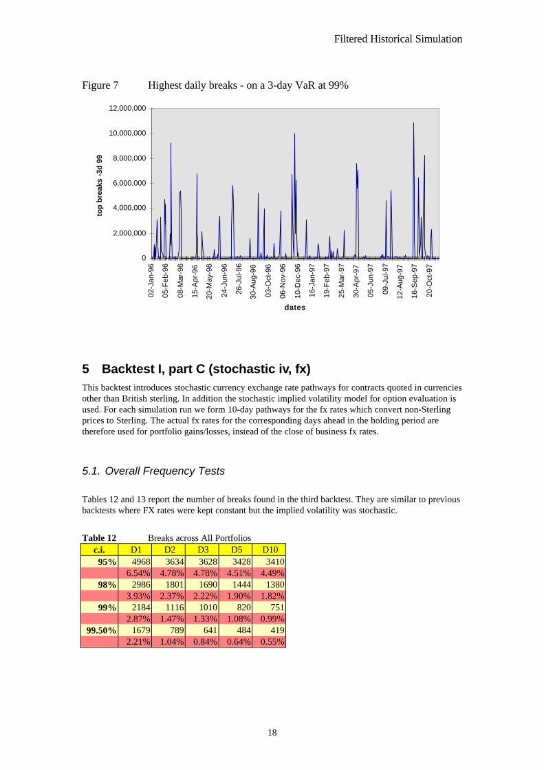
Figure 7 Highest daily breaks - on a 3-day VaR at 99%

0

2,000,000

4,000,000

6,000,000

8,000,000

10,000,000

12,000,000

02-J

an-9

6

05-F

eb-9

6

08-M

ar-9

6

15-A

pr-9

6

20-M

ay-9

6

24-J

un-9

6

26-J

ul-9

6

30-A

ug-9

6

03-O

ct-9

6

06-N

ov-9

6

10-D

ec-9

6

16-J

an-9

7

19-F

eb-9

7

25-M

ar-9

7

30-A

pr-9

7

05-J

un-9

7

09-J

ul-9

7

12-A

ug-9

7

16-S

ep-9

7

20-O

ct-9

7

dates

top

bre

aks

-3d

99

5 Backtest I, part C (stochastic iv, fx) This backtest introduces stochastic currency exchange rate pathways for contracts quoted in currenciesother than British sterling. In addition the stochastic implied volatility model for option evaluation isused. For each simulation run we form 10-day pathways for the fx rates which convert non-Sterlingprices to Sterling. The actual fx rates for the corresponding days ahead in the holding period aretherefore used for portfolio gains/losses, instead of the close of business fx rates.

5.1. Overall Frequency Tests

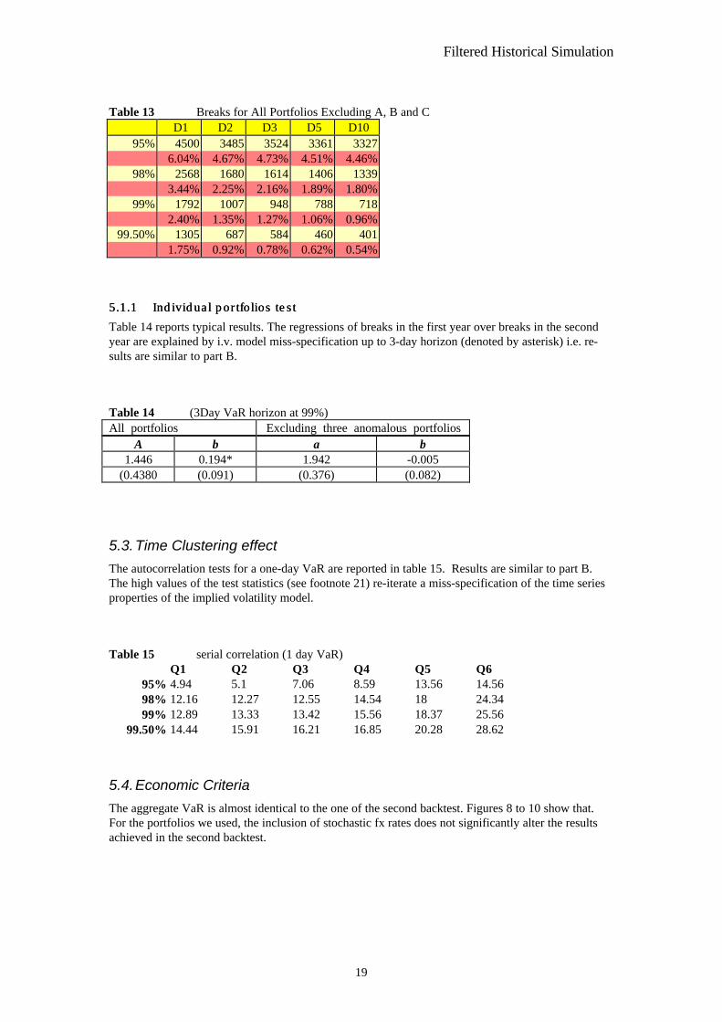
Tables 12 and 13 report the number of breaks found in the third backtest. They are similar to previousbacktests where FX rates were kept constant but the implied volatility was stochastic.

Table 12 Breaks across All Portfolios c.i. D1 D2 D3 D5 D10 95% 4968 3634 3628 3428 3410

6.54% 4.78% 4.78% 4.51% 4.49% 98% 2986 1801 1690 1444 1380

3.93% 2.37% 2.22% 1.90% 1.82% 99% 2184 1116 1010 820 751

2.87% 1.47% 1.33% 1.08% 0.99% 99.50% 1679 789 641 484 419

2.21% 1.04% 0.84% 0.64% 0.55%


19

Table 13 Breaks for All Portfolios Excluding A, B and C

D1 D2 D3 D5 D10 95% 4500 3485 3524 3361 3327

6.04% 4.67% 4.73% 4.51% 4.46% 98% 2568 1680 1614 1406 1339

3.44% 2.25% 2.16% 1.89% 1.80% 99% 1792 1007 948 788 718

2.40% 1.35% 1.27% 1.06% 0.96% 99.50% 1305 687 584 460 401

1.75% 0.92% 0.78% 0.62% 0.54%

5.1.15.1.1 Individual portfolios testIndividual portfolios test

Table 14 reports typical results. The regressions of breaks in the first year over breaks in the secondyear are explained by i.v. model miss-specification up to 3-day horizon (denoted by asterisk) i.e. re-sults are similar to part B.

Table 14 (3Day VaR horizon at 99%)

A b a b 1.446 0.194* 1.942 -0.005

(0.4380 (0.091) (0.376) (0.082)

5.3.Time Clustering effect

The autocorrelation tests for a one-day VaR are reported in table 15. Results are similar to part B.The high values of the test statistics (see footnote 21) re-iterate a miss-specification of the time seriesproperties of the implied volatility model.

Table 15 serial correlation (1 day VaR) Q1 Q2 Q3 Q4 Q5 Q6

95% 4.94 5.1 7.06 8.59 13.56 14.56 98% 12.16 12.27 12.55 14.54 18 24.34 99% 12.89 13.33 13.42 15.56 18.37 25.56

99.50% 14.44 15.91 16.21 16.85 20.28 28.62

5.4.Economic Criteria

The aggregate VaR is almost identical to the one of the second backtest. Figures 8 to 10 show that.For the portfolios we used, the inclusion of stochastic fx rates does not significantly alter the resultsachieved in the second backtest.

All portfolios Excluding three anomalous portfolios


20

Figure 8 Sum of ten largest breaks on 10 day VaR at 99%

0

5000000

10000000

15000000

20000000

25000000

30000000

35000000

40000000

45000000

50000000

02-J

an-9

6

09-F

eb-9

6

20-M

ar-9

6

01-M

ay-9

6

12-J

un-9

6

22-J

ul-9

6

30-A

ug-9

6

09-O

ct-9

6

18-N

ov-9

6

30-D

ec-9

6

07-F

eb-9

7

19-M

ar-9

7

30-A

pr-9

7

11-J

un-9

7

21-J

ul-9

7

29-A

ug-9

7

08-O

ct-9

7

date

loss

es

Figure 9 Total VaR on 10 Days at 99%

0

500,000,000

1,000,000,000

1,500,000,000

2,000,000,000

2,500,000,000

3,000,000,000

02-J

an-9

6

13-F

eb-9

6

26-M

ar-9

6

10-M

ay-9

6

24-J

un-9

6

05-A

ug-9

6

17-S

ep-9

6

29-O

ct-9

6

10-D

ec-9

6

24-J

an-9

7

07-M

ar-9

7

22-A

pr-9

7

05-J

un-9

7

17-J

ul-9

7

29-A

ug-9

7

10-O

ct-9

7

Date

To

tal V

aR


21

Figure 10 Largest Daily Break for a 3 Days VaR at 99%

0

2000000

4000000

6000000

8000000

10000000

12000000

02-J

an-9

6

09-F

eb-9

6

20-M

ar-9

6

01-M

ay-9

6

12-J

un-9

6

22-J

ul-9

6

30-A

ug-9

6

09-O

ct-9

6

18-N

ov-9

6

30-D

ec-9

6

07-F

eb-9

7

19-M

ar-9

7

30-A

pr-9

7

11-J

un-9

7

21-J

ul-9

7

29-A

ug-9

7

08-O

ct-9

7

Date

To

p B

reak

-3D

ays


22

Section 2: Backtesting on Swaps

6 The Swaps Backtesting methodology Following the FHS methodology, for each trading day and each currency we simulate 5000 scenariosfor 14 factors from the zero curve based on maturities from overnight (ON) to 10 years (10Y), (1W,1M, 2M, 3M, 6M, 9M, 12M, 2Y, 3Y, 4Y, 5Y, 7Y, 10Y). On each scenario we price all swaps.Therefore, for each factor23 5000 forecasts are generated using that factor’s own volatility estimatesand historical daily returns. One of the advantages of our approach is to allow the near end of theyield curve to be more volatile than the far end. On the other hand the (parallel) bootstrapping used inFHS provides the means to capture the interdependence between factors across the term structure andalso across other currency rates and different financial instruments24.

We use daily money and coupon rates (swap)25 for four currencies for the period 2 January 1994 to 10November 1997. The first two years’ data set is used as in-sample database, and provides the feed forour historical simulation. Therefore our backtests start on the first trading date of 1996. At each busi-ness date and for each of the four swap portfolios and their currency components we generate 5000simulated prices for days 1, 2, 3, 5, and 10. The risk measure is determined directly for the desiredpercentile (e.g. 99th percentile) from the distribution of 5000 portfolio (simulated) values for a givennumber of days ahead in the VaR period.

A break occurs when:

Pa,t+i < Mint+i

where Pa,t+i is the portfolio’s actual value at the ith VaR day ahead in the holding period and Mint+i thelower predicted value for that probability level.

In order for FHS to meet the statistical criteria the difference in the number of breaks from their ex-pected value must be statistically insignificant (i.e. at 95% probability on average we will have 5breaks for a portfolio over 100 days.

6.1 Expiring Swaps and Coupons

It is important that the portfolios remain identical over the VaR horizon for each business date duringthe backtest. To satisfy this, for each business day we run FHS we use the following rules:

23 For a trading date we generated risk measures for 1 to 10 days ahead. Hence for each zero rate fac-tor 5000 ten-day pathways were created. 24 See Barone-Adesi, Giannopoulos and Vosper (1999) for a description of how BAGV takes into ac-count the possible daily co-movements between different financial instruments. 25 The data providers are Olsen Associates (money rates) and Dart (swap rates).


23

• SWAP contracts that expire on the close of business26 are not included in the portfolio (i.e. con-tracts with positions having zero days to expiry).

• SWAP contracts that expire the next day are not included in the portfolio (i.e. contracts with po-sitions having one day to expiry).

• Coupons paid during the holding period are ignored (added back) to ensure comparability of re-sults.

• Swap contracts, which expire between 2 and 10 days inclusive during the holding period, haveprevious day values in the pathways “frozen in” as done in section 1.

• Actual portfolio values are calculated to reflect the above treatment e.g. a swap’s actual closingprice one day prior to its expiry date is “copied forward” to the expiry date and subsequent datesuntil the last day of the VaR horizon. This is done to ensure that marking to market is done con-sistently with FHS.

7 Backtest on 24 small SWAP booksThree sets of backtests are performed. For the first two the same set of 24 portfolios mixed across thefour currencies are employed. In the third backtest we use four currency mixed portfolios consisting of500 swaps each. The scope of the third backtest is to investigate the effects of diversification in largerswap portfolios and to analyse the portfolios that will provide the swap components for the finalcombo backtest. During the first backtest we translate all returns to Sterling at the close of businessFX rates. The scope of the second backtest is to investigate the impact of currency risk. Therefore,during the second backtest we generate pathways for both currency-to-Sterling FX rates and zero cou-pon rates27. The third backtest is run with stochastic FX.

7.1.17.1.1 Overall frequency testsOverall frequency tests

A break occurs when the portfolio trading loss is greater than the one predicted by FHS for that VaRhorizon. On Table 16, we show the number of breaks across the 24 portfolios for the 2-year period(total of 11,639 daily portfolios)28. The number of breaks recorded across all portfolios for the entirebacktest period are reported in each column, D1, D2, D3, D5, D10, to denote the 1, 2, 3, 5 and 10 dayVaR horizons.

We record the breaks for four confidence levels (percentiles), 95%, 98%, 99% and 99.5%. Below eachnumber of breaks we report the corresponding percentage on the number of predictions. The expectednumber for those percentages should be equal to one minus the corresponding confidence level.

26 We refer to the “close of business” date as the date for which we ran the simulation.27 Simulated pathways for the FX rates have been generated in the same way as those of the yieldrates. The correlation between the former and latter was preserved with the parallel bootstrapping.28 For the last 311 days of the first two backtests, there was an additional portfolio.

Table 16 Breaks across 24 Portfolios (Constant FX)c.i. D1 D2 D3 D5 D10

95% 495 515 511 496 4114.25% 4.42% 4.39% 4.26% 3.53%

98% 234 217 227 203 1362.01% 1.86% 1.95% 1.74% 1.17%

99% 133 131 134 109 671.14% 1.13% 1.15% 0.94% 0.58%

99.5% 90 90 85 66 320.77% 0.77% 0.73% 0.57% 0.27%


24

In table 17 we report the number of breaks and the percentages breaks on the same portfolios. Thistime the FX rates as well as the yield factors are forecast.

Table 17 Breaks across 24 Portfolios (Stochastic FX)c.i. D1 D2 D3 D5 D1095% 519 518 505 479 412

4.46% 4.45% 4.34% 4.12% 3.54%98% 233 219 235 214 125

2.00% 1.88% 2.02% 1.84% 1.07%99% 143 133 142 113 70

1.23% 1.14% 1.22% 0.97% 0.60%99.5% 97 91 85 66 39

0.83% 0.78% 0.73% 0.57% 0.34%

Results in Tables 16 and 17 show that FHS tends to over-estimate risk slightly. This effect is morepronounced at long horizons. Clearly most table values at short horizons are not significantly differentfrom theoretical values. At longer horizons FHS becomes too conservative. There is no significantdifference, in the risk prediction, between the first (constant FX) and second (stochastic FX) backtest.

7.1.27.1.2 Individual Portfolio TestsIndividual Portfolio Tests

Individual portfolio tests try to determine whether breaks occur randomly in our sample. Clusters ofbreaks indicate portfolios for which risk may be miss-specified. Under the null hypothesis of random-ness the number of breaks in the two halves of our backtesting period are independent. Therefore across-sectional regression of the breaks reported for each firm in the first half on the number of breaksreported in the second half should have zero slope (i.e. b=0).

The regression analysis on the breaks for each sub-period in Table 18 confirms that the slope, b, is notsignificant. There is therefore no evidence of FHS failing to capture the risk of any of our tested port-folios.

Table 18 (3-Day VaR horizon at 99%)24 portfolios - constant FX 24 portfolios - stochastic FX

A B a b3.176* -0.219 2.659* -0.023(1.023) (0.278) (0.970) (0.242)

(numbers in brackets are standard errors)

7.1.37.1.3 Time clustering effectTime clustering effect

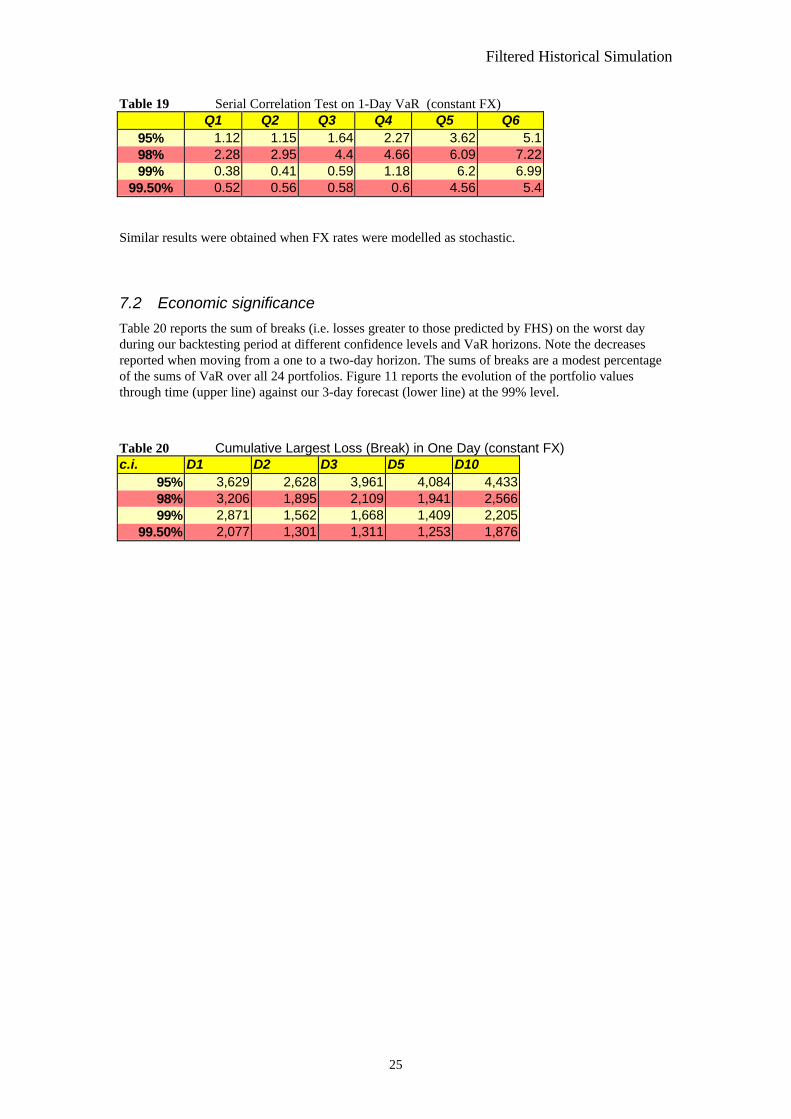
Clustering tests assess whether days with large number of breaks across all the firms tend to be fol-lowed by other days with large numbers of breaks, pointing to a miss-specification of the time-seriesmodel of volatility. The evidence of that can be detected by the autocorrelations in the aggregate num-ber of breaks occurring each day. The results are displayed in table 19; there is no evidence of signifi-cant serial correlations29 (order 1 to 6) for any confidence level at the 1 day VaR horizon30.

29 At the 95% level, the critical value for the Chi-square test is 12.6.30 The overlapping of measurement intervals makes this test not applicable at longer horizons, becauseportfolios can no longer be regarded as being independent.


25

Table 19 Serial Correlation Test on 1-Day VaR (constant FX)Q1 Q2 Q3 Q4 Q5 Q6

95% 1.12 1.15 1.64 2.27 3.62 5.198% 2.28 2.95 4.4 4.66 6.09 7.2299% 0.38 0.41 0.59 1.18 6.2 6.99

99.50% 0.52 0.56 0.58 0.6 4.56 5.4

Similar results were obtained when FX rates were modelled as stochastic.

7.2 Economic significance

Table 20 reports the sum of breaks (i.e. losses greater to those predicted by FHS) on the worst dayduring our backtesting period at different confidence levels and VaR horizons. Note the decreasesreported when moving from a one to a two-day horizon. The sums of breaks are a modest percentageof the sums of VaR over all 24 portfolios. Figure 11 reports the evolution of the portfolio valuesthrough time (upper line) against our 3-day forecast (lower line) at the 99% level.

Table 20 Cumulative Largest Loss (Break) in One Day (constant FX)c.i. D1 D2 D3 D5 D10

95% 3,629 2,628 3,961 4,084 4,43398% 3,206 1,895 2,109 1,941 2,56699% 2,871 1,562 1,668 1,409 2,205

99.50% 2,077 1,301 1,311 1,253 1,876


26

Figure 11 Forecast vs. Actual (Forecast at 99% Probability for a 3-day Horizon)

F o r e c a s t A c t u a l

27/1

0/19

97

27/0

9/19

97

28/0

8/19

97

29/0

7/19

97

29/0

6/19

97

30/0

5/19

97

30/0

4/19

97

31/0

3/19

97

01/0

3/19

97

30/0

1/19

97

31/1

2/19

96

01/1

2/19

96

01/1

1/19

96

02/1

0/19

96

02/0

9/19

96

03/0

8/19

96

04/0

7/19

96

04/0

6/19

96

05/0

5/19

96

05/0

4/19

96

06/0

3/19

96

05/0

2/19

96

06/0

1/19

96

VA

lue(

x000

s)

7 , 3 3 2 . 8

6 , 4 1 6 . 2

5 , 4 9 9 . 6

4 , 5 8 3

3 , 6 6 6 . 4

2 , 7 4 9 . 8

1 , 8 3 3 . 2

9 1 6 . 6

0

- 9 1 6 . 6

- 1 , 8 3 3 . 2

- 2 , 7 4 9 . 8

- 3 , 6 6 6 . 4

8 Backtest on four large swap portfolios.Part C of backtest II is run on four large swap portfolios. Each of these portfolios consists of swaps inall four currencies. They differ in terms of maturity and type of position (pay or receivefixed/floating). The data sample used in the backtest is a sample of large swap books provided byanonymous banks. Table 21 describes these portfolios.

Table 21 Portfolio DescriptionPortfolio Duration Position1 Any Pay fixed2 short Pay fixed/float3 medium Pay fixed/float4 any Pay fixed/float

The analysis for the breaks across our four portfolios is shown in table 22. As in the first two back-tests, violations on the FHS predictions tend to be in line with the probability level for short horizons.For longer horizons, FHS tends to be conservative (over-estimates risk). However the limited numberof portfolios leads to large fluctuations in the frequency of breaks, ranging up to 1%.


27

Table 22 Breaks across Four Portfolios D1 D2 D3 D5 D10

95% 72 81 79 65 513.81% 4.29% 4.18% 3.44% 2.70%

98% 36 38 29 24 111.91% 2.01% 1.54% 1.27% 0.58%

99% 25 20 21 9 41.32% 1.06% 1.11% 0.48% 0.21%

99.50% 17 9 3 2 00.90% 0.48% 0.16% 0.11% 0.00%

To investigate whether the results are uniform across the different currencies we break down the fourportfolios into the four currency components. Tables 23-26 report the breaks and percentage breaksfor each currency component.

Table 23 Breaks across all DEM Portfolios D1 D2 D3 D5 D10

95% 67 72 77 76 623.55% 3.81% 4.08% 4.03% 3.28%

98% 30 32 42 25 231.59% 1.70% 2.23% 1.32% 1.22%

99% 20 18 18 13 51.06% 0.95% 0.95% 0.69% 0.27%

99.50% 13 12 7 7 20.69% 0.64% 0.37% 0.37% 0.11%

Table 24 Breaks across all GBP Portfolios D1 D2 D3 D5 D10

95% 58 46 59 49 343.07% 2.44% 3.13% 2.60% 1.80%

98% 17 21 20 19 60.90% 1.11% 1.06% 1.01% 0.32%

99% 10 9 7 11 10.53% 0.48% 0.37% 0.58% 0.05%

99.50% 6 3 3 5 00.32% 0.16% 0.16% 0.27% 0.00%


28

Table 25 Breaks across all JPY Portfolios D1 D2 D3 D5 D10

95% 116 81 84 98 776.14% 4.29% 4.45% 5.19% 4.08%

98% 40 36 38 44 152.12% 1.91% 2.01% 2.33% 0.79%

99% 27 25 32 22 81.43% 1.32% 1.70% 1.17% 0.42%

99.50% 22 19 23 10 21.17% 1.01% 1.22% 0.53% 0.11%

Table 26 Breaks across all USD Portfolios D1 D2 D3 D5 D10

95% 81 73 78 54 434.29% 3.87% 4.13% 2.86% 2.28%

98% 33 26 32 20 111.75% 1.38% 1.70% 1.06% 0.58%

99% 20 21 17 12 31.06% 1.11% 0.90% 0.64% 0.16%

99.50% 13 15 9 4 10.69% 0.79% 0.48% 0.21% 0.05%

Again, our results confirm that the frequency of breaks on FHS risk predictions closely matches thecorresponding confidence level across all currencies examined. There is however, a tendency to un-der-estimate risk on the JPY book for short horizons. This is not a surprise since there is a dramaticdrop on Japanese rates during the second half of the backtest period. Nevertheless this is correctedafter few days (on three or longer day horizon). On ten days FHS becomes conservative even for theJPY book.


29

Section 3: Backtesting on CombinedPortfolios

9 Data and methodologyIn this final section we analyse the results of backtests performed on 20 portfolios consisting of swapsand interest rate futures and options traded on LIFFE . We combine our four large swap portfolioswith 20 portfolios used in the futures and options backtests (see section I). Each swap portfolio istherefore assigned to 5 members. To make the risks for swap and option positions comparable, all thenotional amounts of swap contracts are scaled31.

9.1 The Data

Our data consist of LIFFE futures and options prices and money and coupon rates (swap) and coverthe period from 2 January 1994 to 10 November 199732. The first two years of our data set is used asan in-sample database and provides the feed for our historical simulation.

We begin our backtest on the 2nd January 1996 and for each consecutive business date up to 10th No-vember 1997, use FHS to make predictions (pathways), for 1 to 10 days ahead, for all the futures andoptions33 contracts traded on that date. Parallel to these predictions we generate the pathways formoney and coupon rates; these pathways are used to price each of the 2000 swaps in the database. Wethen apply the futures and options pathways to each of the futures and options positions34. The result-ing values are added to the swap simulated prices to compute the pathways for the combo portfolio35.The risk measure is determined directly for the desired percentile (e.g. 99th percentile) from the distri-bution of 5000 portfolio (simulated) values for the desired VaR horizon.

A break occurs when:

Pa,t+i < Mint+i

where Pa,t+i is the portfolio’s actual value at the ith VaR day ahead in the holding period and Mint+i thelower predicted value for that probability level.

31 We found that by multiplying all swap notionals by a factor of 10, the risk of our 20 portfolios isapproximately equally balanced between swaps and interest rate futures and options.32 For a full description see sections I and II.33 The approach we use to form the pathways for the options is the one followed in the 3rd backtest forLIFFE, stochastic implied volatility and stochastic FX.34 A full description on how we handled the expiring contracts is provided in the previous sections.35 We apply the FX risk to the market value of the swap portfolio. That assumes that the risk is meas-ured in the domestic currency regardless of the swap currency.


30

10 Backtesting ResultsOne set of backtests is performed where the fx rates and implied volatilities are forecast in parallelwith the futures, option and swap prices36. Since all twenty portfolios are currency-mixed, all forecastprices are translated to GBP using the stochastic FX rates. Similarly, to calculate the breaks we trans-late all actual contract and swap prices to GBP. The statistical results are reported in this section.

10.1 Overall frequency tests

A break occurs when the portfolio trading loss is greater than the one predicted by FHS for that VaRhorizon. In Table 27, we show the number of breaks across the 20 mixed portfolios for the 2-year pe-riod (total of 9,440 daily portfolios). The number of breaks recorded across all portfolios for the entirebacktest period are reported in each column, D1, D2, D3, D5, D10, to denote the 1, 2, 3, 5 and 10 dayVaR horizons.

We record the breaks at four confidence levels (percentiles), 95%, 98%, 99% and 99.5%. Below eachnumber of breaks we report the corresponding percentage on the number of predictions. The expectednumber of breaks at each confidence level should be equal to one minus the corresponding confidencelevel.

D1 D2 D3 D5 D1095% 402 419 395 321 281

4.26% 4.44% 4.18% 3.40% 2.98%98% 203 178 149 117 79

2.15% 1.89% 1.58% 1.24% 0.84%99% 126 92 77 50 32

1.34% 0.98% 0.82% 0.53% 0.34%99.50% 82 41 32 19 10

0.87% 0.43% 0.34% 0.20% 0.11%

Most table values at short horizons are not significantly different from theoretical values. However, atlonger horizons FHS becomes too conservative.

10.2 Time clustering effect

The results of tests of clustering are displayed in table 33; there is no evidence of significant serialcorrelation (order 1 to 6) in the numbers of daily breaks for any confidence level at the 1 day VaRhorizon.

Table 28 Serial Correlation Test on 1-Day VaR (constant FX)Q1 Q2 Q3 Q4 Q5 Q6

95% 0.94 2.72 3.77 4.01 4.28 4.9598% 0.72 1.54 1.76 2.02 2.72 3.3399% 0.59 1.02 1.25 1.48 1.88 2.42

99.50% 0.30 0.60 0.70 0.86 2.15 2.42

36 Stochastic FX and i.v.

Table 27 Breaks across All Portfolios (LIFFE+Swaps)


31

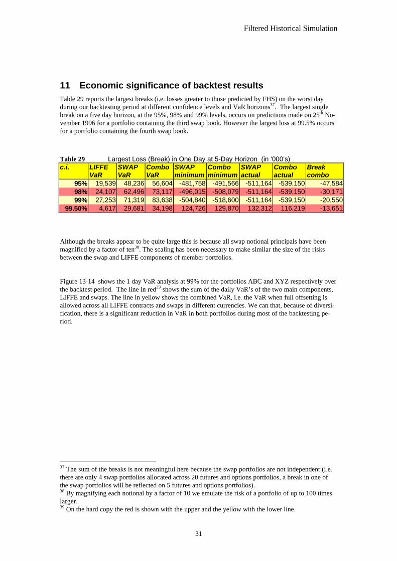
11 Economic significance of backtest resultsTable 29 reports the largest breaks (i.e. losses greater to those predicted by FHS) on the worst dayduring our backtesting period at different confidence levels and VaR horizons37. The largest singlebreak on a five day horizon, at the 95%, 98% and 99% levels, occurs on predictions made on 25th No-vember 1996 for a portfolio containing the third swap book. However the largest loss at 99.5% occursfor a portfolio containing the fourth swap book.

Table 29 Largest Loss (Break) in One Day at 5-Day Horizon (in ‘000’s)c.i. LIFFE

VaRSWAPVaR

ComboVaR

SWAPminimum

Combominimum

SWAPactual

Comboactual

Breakcombo

95% 19,539 48,236 56,604 -481,758 -491,566 -511,164 -539,150 -47,58498% 24,107 62,496 73,117 -496,015 -508,079 -511,164 -539,150 -30,17199% 27,253 71,319 83,638 -504,840 -518,600 -511,164 -539,150 -20,550

99.50% 4,617 29,681 34,198 124,726 129,870 132,312 116,219 -13,651

Although the breaks appear to be quite large this is because all swap notional principals have beenmagnified by a factor of ten38. The scaling has been necessary to make similar the size of the risksbetween the swap and LIFFE components of member portfolios.

Figure 13-14 shows the 1 day VaR analysis at 99% for the portfolios ABC and XYZ respectively overthe backtest period. The line in red39 shows the sum of the daily VaR’s of the two main components,LIFFE and swaps. The line in yellow shows the combined VaR, i.e. the VaR when full offsetting isallowed across all LIFFE contracts and swaps in different currencies. We can that, because of diversi-fication, there is a significant reduction in VaR in both portfolios during most of the backtesting pe-riod.

37 The sum of the breaks is not meaningful here because the swap portfolios are not independent (i.e.there are only 4 swap portfolios allocated across 20 futures and options portfolios, a break in one ofthe swap portfolios will be reflected on 5 futures and options portfolios).38 By magnifying each notional by a factor of 10 we emulate the risk of a portfolio of up to 100 timeslarger.39 On the hard copy the red is shown with the upper and the yellow with the lower line.


32

Figure 12 VaR analysis for portfolio ABC (1-day var. at 99%)

Figure 13 VaR analysis for portfolio XYZ (1-day var. at 99%)

LIffe+Swap VaR Liffe VaR

27

/10

/97

27

/09

/97

28

/08

/97

29

/07

/97

29

/06

/97

30

/05

/97

30

/04

/97

31

/03

/97

01

/03

/97

30

/01

/97

31

/12

/96

01

/12

/96

01

/11

/96

02

/10

/96

02

/09

/96

03

/08

/96

04

/07

/96

04

/06

/96

05

/05

/96

05

/04

/96

06

/03

/96

05

/02

/96

06

/01

/96

Va

lue

s

35,000,000

30,000,000

25,000,000

20,000,000

15,000,000

10,000,000

5,000,000

0

LIffe+Swap VaR Liffe VaR

27/1

0/9

7

27/0

9/9

7

28/0

8/9

7

29/0

7/9

7

29/0

6/9

7

30/0

5/9

7

30/0

4/9

7

31/0

3/9

7

01/0

3/9

7

30/0

1/9

7

31/1

2/9

6

01/1

2/9

6

01/1

1/9

6

02/1

0/9

6

02/0

9/9

6

03/0

8/9

6

04/0

7/9

6

04/0

6/9

6

05/0

5/9

6

05/0

4/9

6

06/0

3/9

6

05/0

2/9

6

06/0

1/9

6

Valu

es

55,000,000

50,000,000

45,000,000

40,000,000

35,000,000

30,000,000

25,000,000

20,000,000

15,000,000

10,000,000

5,000,000

0


33

12 Offsetting risk across contracts and currenciesOne of the features of FHS is to account for the benefits of risk diversification across different con-tracts and currencies (swaps). The proportion of risk reduced because of diversification can be meas-ured as follows:

VaR

VaR VaR VaR VaR VaR VaR VaR VaR VaR VaR VaRt combo

t A t C t G t L t S t U t W t DEM t GBP t JPY t USD

,

, , , , , , , , , , ,+ + + + + + + + + +

where VaRt combo, is the VaR calculated for day t on the mixed portfolio as described in section 1.

VaRt A, ,…VaRt W, are the VaR of positions on contracts A to W (LIFFE) for that probability level

and investment horizon. The analogous swap (currency) components in each portfolio are shown asVaRt DEM, ,… VaRt USD, . After multiplying each of the eleven VaR numbers by the corresponding

GBP FX rate we add them together to create a new series of daily VaR values, as in the denominatorof the above ratio. Each of these aggregated daily values reflects the risk associated with the relevantportfolio; we denote this as undiversified risk40.

40 This happens under the extreme hypothesis that worst losses (e.g. at 99%) for each LIFFE contractand swap book all occur simultaneously.


34

Figure 14 Risk Ratio (5-day var. at 99%) for portfolio ABC

Figure 15 Risk Ratio41 (5 day VaR @ 99%) for portfolio XYZ

Figures 14 and 15 show the proportion of the combo VaR over the aggregated VaR of individual com-ponents of all LIFFE contracts and a single currency swap book for a 5-day VaR at 99%. There is a 41 This is the VaR of the combo portfolio over the sum of VaR components.

27

/10

/97

27

/09

/97

28

/08

/97

29

/07

/97

29

/06

/97

30

/05

/97

30

/04

/97

31

/03

/97

01

/03

/97

30

/01

/97

31

/12

/96

01

/12

/96

01

/11

/96

02

/10

/96

02

/09

/96

03

/08

/96

04

/07

/96

04

/06

/96

05

/05

/96

05

/04

/96

06

/03

/96

05

/02

/96

06

/01

/96

Va

lue

s

1

0.9

0.8

0.7

0.6

0.5

0.4

0.3

0.2

0.1

0

27/1

0/97

27/0

9/97

28/0

8/97

29/0

7/97

29/0

6/97

30/0

5/97

30/0

4/97

31/0

3/97

01/0

3/97

30/0

1/97

31/1

2/96

01/1

2/96

01/1

1/96

02/1

0/96

02/0

9/96

03/0

8/96

04/0

7/96

04/0

6/96

05/0

5/96

05/0

4/96

06/0

3/96

05/0

2/96

06/0

1/96

Val

ues

1

0.9

0.8

0.7

0.6

0.5

0.4

0.3

0.2

0.1

0


35

large reduction in risk. In a portfolio the combo VaR can be as low as 20% of the aggregated VaR’s.The proportion of risk that is reduced because of diversification is given by 1 minus the above ratio.

13 ConclusionsThe results of the three backtests on futures and options indicate that FHS provides an effectiveframework to measure risk of portfolios of interest rate futures and options. No version of FHS domi-nates alternative versions in every dimension. Therefore actual implementations should be based oncareful consideration of management priorities.

There seems to be little room for improvement in the results of the first backtest, keeping impliedvolatilities constant. The results of the first backtest are adequate except for the three identified port-folios. However these portfolios are subject to risks that do not fit well in the constant volatilityframework.

The second backtest suggests that the stochastic implied volatility model is adequate at long horizons(5 or 10 days). However there is room from improvement of the methodology of the second backtest toreduce clustering of breaks or to improve its performance at short horizons. It is unlikely that thesepotential improvements would lead to further reductions in break size in the worst days beyond thelarge ones already observed in our backtest.

The third backtest does not alter the above conclusions. This is to be expected with the futures andoptions contracts, where currency exchange risk is small.

It is important to remember that our backtest results are based on comparing the VaR value withportfolio profits (losses) on the same horizon (e.g. 3 day VaR vs 3 day portfolio profits /losses). Nocash settlement-to-market is allowed for within the VaR horizon. In practice however, FHS VaRnumbers at longer horizons could be used to monitor daily risk. Breaks would be very rare when com-pared to portfolio profits/losses under daily cash settlement to market.

Our swap backtest evaluate the risk of plain vanilla swaps on four currencies (DEM, GBP, JPY, andUSD) and for (residual) maturities ranging from 2 days to 10 years. We ran daily simulations onmixed and single currency portfolios for a period of nearly 2 years. Our results indicate that errors inFHS predictions are agreeable with the pre-set VaR probability levels. We find a tendency in FHS toover-estimate risk at longer horizons. The results do not change between single and multi-currencyportfolios. The analysis of the risk diversification reveals that a significant amount of risk (in somecases as much as 66% on selected days) is eliminated through diversification across currencies.

Finally, we backtest portfolios invested in interest rate futures and options and plain vanilla swaps.There was no major difficulty in simulating futures, options and swaps using consistent pathways. Theoverall results show that FHS is accurate at shorter horizons, but tends to become conservative at longhorizons, as previously reported for swaps. The fact that VaR values are more stable for swaps thanfor futures and options may be partly due to our choice of portfolios, but the lack of secondary marketsfor swaps may contribute to that. Managers in fact may implement their active strategies more easilyin markets that allow for secondary trading. In all cases it appears that significant risk diversificationis achieved. In fact combining swaps and futures portfolios cuts up to 70-80% of risk.Our extensive testing suggests that filtered historical simulation, introduced in FHS, is capable ofmodelling market risk accurately for portfolios of derivative contracts.


36

BIBLIOGRAPHY

Barone-Adesi G, F Bourgoin and K Giannopoulos (1998), “Don’t Look Back”,Risk, 11, August, 100-104.

Barone-Adesi G and K Giannopoulos (1996), “A Simplified Approach to theConditional Estimation of Value at Risk”, Futures and Options World, Oc-tober, 68-72.

Barone-Adesi G, K Giannopoulos and L Vosper (1999), “VaR Without Correla-tions for non-linear Portfolios”, Journal of Futures Markets, 19, August,583-602.

Basle Committee on Banking Supervision (1996), Supervisory Framework forthe Use of Backtesting in conjunction with the Internal Models Approach toMarket Risk Capital Requirements, Basle.

Bollerslev T (1986), “Generalised Autoregressive Conditional Heteroskedastic-ity”, Journal of Econometrics, 31, 307-327.

Butler J S and B Schachter (1998), “Estimating Value at Risk by CombiningKernel Estimation with Historical Simulation, Review of Derivatives Re-search, 1, 371-390.

Kendall M (1953), "The Analysis of Economic time-Series", Journal of theRoyal Statistical Society, 96, 11-25.

Jamshidian F and Y Zhu (1997), “Scenario Simulation Model: Theory and Meth-odology”, Finance and Stochastics, 1, 43-67.

Ljung G.M. and G.E.P. Box (1978), “On a Measure of Lack of Fit in Time Se-ries Models”, Biometrika, 67, 297-303.

Mandelbrot B (1963), “The Variation of Certain Speculative Prices”, Journal ofBusiness, 36, 394-419.

Markowitz H (1959), Portfolio Selection: Efficient Diversification of Invest-ments, John Wiley, NY.

RiskMetrics, (1993), 1st edition, JP Morgan publication.

filtering historical simulation. backtest analysis · filtered historical simulation 1 filtering...

Documents