fin 30220: macroeconomics labor markets. the us labor market by the numbers…* total population...
TRANSCRIPT

FIN 30220: Macroeconomics
Labor Markets

The US Labor Market by the numbers…*
Total Population
321M
“Ineligible to work”
71M
• Under 16 years old• Inmates of institutions (penal,
mental, homes for the aged)• Active duty military
Employed
149M
*As reported by the household survey (Bureau of Labor Statistics)
Unemployed
8.5MNot Participating
92.5M
• To be considered “unemployed”, you must have looked for work over the last 30 days. Otherwise, you are “not participating”

Total Population
321M
“Ineligible to work”
71M
Employed
149M
Unemployed
8.5MNot Participating
92.5M
The US Labor Market by the numbers…*
*As reported by the household survey (Bureau of Labor Statistics)
Civilian Employment-Population Ratio
Total employment divided by the eligible population
Eligible Population = Employed + Unemployed + Not Participating149
250*100 = 59.6%
“Official” Unemployment Rate (U-3)
Unemployment divided by the Labor Force
Labor Force = Employed + Unemployed
8.5157.5
*100 = 5.4%
Participation Rate
labor force divided by the eligible population
157.5 *100 = 63%250

1948 1953 1958 1963 1968 1973 1978 1983 1988 1993 1998 2003 2008 20130.0
2.0
4.0
6.0
8.0
10.0
12.0
NBER Recession Dates
Une
mpl
oym
ent R
ate
Unemployment in the US
*Source: Bureau of Labor Statistics
Non Recession Average: 5.8%Recession Average: 6.1%
Current = 5.5%
December 198210.8%
May 19532.5%

To be considered “employed” you only need to have a job (no distinction between full time or part time)To be considered “unemployed”, you must have looked for work over the last 30 days. Otherwise, you are “not participating”.
Alternate Measures of Unemployment in the U.S.
Discouraged Workers
• Persons who are not in the labor force
• Want to and are available to work
• Have looked for work over the year, but not over the last 4 weeks
• Specific reason cited for not looking for work is that they don’t believe there is a job available
Marginally Attached Workers
• Persons who are not in the labor force
• Want to and are available to work
• Have looked for work over the year, but not over the last 4 weeks
• Any reason cited for lack of job search
Part Time for Economic Reasons
• Working less than 35 hours per week
• Want to and are available to work full time
• Gave an economic reason (Hours cut, unable to find full time work) for lack of a full time job

Alternate Measures of Unemployment in the U.S.
*From the latest household survey, BLS
Category May 2014
Eligible Population 250M
Labor Force 157.5M
Employed 149M
Unemployed 8.5M
Discouraged Workers 600,000
Marginally Attached Workers 1.8M
Part time for Economic Reasons 6.6M
U-4 Unemployment Rate
Unemployed plus discouraged workers divided by the labor force plus discouraged workers
9.1158.1
*100 = 5.8%
U-5 Unemployment Rate
Unemployed plus discouraged workers plus marginally attached divided by the Labor Force + discouraged workers + marginally attached
10.9159.9
*100 = 6.8%
U-6 Unemployment Rate
Unemployed plus discouraged workers plus marginally attached workers plus part time for economic reasons divided by the Labor Force + discouraged workers + marginally attached workers
17.5159.9
*100 = 10.9%
Recall, the “official” (U-3) unemployment rate is 5.5%
Note: U-1 unemployment deals with long term unemployment and U-2 deals with temporary jobs

Let’s look at the US over the years since the last recession…
2007 2008 2009 2010 2011 2012 2013 2014 20154.0
5.0
6.0
7.0
8.0
9.0
10.0
11.0Peak = 10.0%October 2009
Current = 5.5%
Recession Recovery
January 20074.6%

2008 2009 2010 2011 2012 2013 2014 2015
-1000
-800
-600
-400
-200
0
200
400
600
Average = -361,000/mo.
Average = 143,000/mo.
Monthly change in payrolls
280,000 in May 2015
8 million jobs lost during the recession
10 million jobs gained since the end of the recession
June 2009

Let’s do a back of the envelope calculation….population grows at around 1.5% per year. Let’s assume everybody enters the workforce at 16 and retires after 45 years.
Now (2015)45 years ago
(1970)
Eligible population = 107M
1.5% x 107M = 1.60M Entering the workforce 1.60M retiring
Eligible population = 208M
1.5% x 205M = 3.12M Entering the workforce
3.12M – 1.60M = 1.52M / 12 = 126,000 per month!
16 years ago(1999)61 Years ago
(1954)
1.60M

8 million jobs lost during the recession
8,000,000 17,000 = 470 months
To get back to “normal”
(~40 years)
156,000 Jobs created- 126,000 to satisfy population growth 33,000 lost jobs recovered per month
2008 2009 2010 2011 2012 2013 2014 2015
-1000
-800
-600
-400
-200
0
200
400
600
June 2009
143,000 Jobs created- 126,000 to satisfy population growth 17,000 lost jobs recovered per month
Average = 143,000/mo.

1981 1982 1983 1984 1985
-600
-400
-200
0
200
400
600
800
1000
1200
Average = -177,000
Average = 265,000
265,000 Jobs created- 123,000 to satisfy population growth 142,000 lost jobs recovered per month
3,000,000 142,000 = 21 months
To get back to “normal”
(~2 years)
3,000,000 jobs lost
For comparison purposes, during the recovery following the 81-82 recession, we created almost twice as many jobs per month

Lets compare the current recession/recovery to the last few
2 years
How can the unemployment rate drop so quickly with so few jobs being created?
Beginning of recovery
Recession Beginning

Recession Recovery
Let’s look at the US over the years since the last recession…
January 2007 October 2009 May 2015
Category Jan 2007
Eligible Population 230M
Labor Force 153M
Employed 146M
Unemployed 7M
Employment Rate 63.5%
Unemployment Rate 4.6%
Participation Rate 66.5%
Category Oct 2009
Eligible Population 237M
Labor Force 154M
Employed 139M
Unemployed 15M
Employment Rate 58.6%
Unemployment Rate 10.0%
Participation Rate 64.9%
Category May 2015
Eligible Population 250M
Labor Force 157.5M
Employed 149M
Unemployed 8.5M
Employment Rate 59.6%
Unemployment Rate 5.5%
Participation Rate 63%
The primary reason for the decline in the unemployment rate over the past 6 years is the drop in labor force participation!
If we had the same participation rate today as we did in 2007, the unemployment rate would be 10.3%!

This decline in labor force participation began it’s decline prior to the last recession…..
1948 1953 1958 1963 1968 1973 1978 1983 1988 1993 1998 2003 2008 201356.0
58.0
60.0
62.0
64.0
66.0
68.0
Recession
Peak = 67.2%January 2001
Peak = 63%Current
Beginning of Women’s Liberation Movement (1967)
59.7%

1948 1958 1968 1978 1988 1998 200830.0
35.0
40.0
45.0
50.0
55.0
60.0
65.0
1948 1958 1968 1978 1988 1998 200866.0
71.0
76.0
81.0
86.0
91.0Labor Participation Rate - Women Labor Participation Rate - Men
The Women’s Liberation movement isn’t 100% of this shift, but it’s a big part!

1948 1958 1968 1978 1988 1998 200860.0
65.0
70.0
75.0
80.0
85.0
1948 1958 1968 1978 1988 1998 200825.0
27.0
29.0
31.0
33.0
35.0
37.0
39.0
41.0
43.0
45.0Labor Participation Rate: 25 - 54 Labor Participation Rate: 55+
Some people claim that the drop is participation is baby boomers taking early retirement…not the case!!

A decline is participation isn’t the only thing “new” about our current situation…
*From the latest household survey, BLS
Category May 2015
Unemployed (5.5%) 8.5M 100%
Less than 5 weeks 2.4M 28%
Between 5 and 14 weeks 2.5M 29%
Between 15 and 26 weeks 1.3M 15%
Over 26 weeks 2.3M 28%
Category Oct 2000
Unemployed (5.3%) 6.6M 100%
Less than 5 weeks 3M 45%
Between 5 and 14 weeks 2.3M 40%
Between 15 and 26 weeks 0.6M 9%
Over 26 weeks 0.7M 6%
< 5 weeks 5-14 weeks 15-26 weeks >26 weeks0
5
10
15
20
25
30
35
< 5 weeks 5-14 weeks 15-26 weeks >26 weeks0
5
10
15
20
25
30
35
40
45
50
*From the Nov. 2000 household survey, BLS

Category May 2015
Unemployed (5.5%) 8.5M
6.5 weeks 2.4M
13 weeks 2.5M
26 Weeks 1.3M
52 weeks 2.3M
Let’s Simplify a little…
AUGFEB MAR APR MAY JUNE JULYJAN SEPT OCT NOV DEC
So, our unemployed looks roughly like this for 2015…
2.3M
1.3M 1.3M
2.5M 2.5M 2.5M 2.5M
2.4M 2.4M 2.4M 2.4M 2.4M 2.4M 2.4M 2.4M
Total = 8.5
Category Total for
2015
% for 2015
Unemployed 34.1M 100%
6.5 weeks 19.2M 56%
13 weeks 10M 29%
26 Weeks 2.6M 8%
52 weeks 2.3M 7%
Duration of Unemployment
.56 6.5 .29 13 .08 26 .07 52 13 D weeks
Length of unemployment spell
% of total unemployed in a year

1948 1953 1958 1963 1968 1973 1978 1983 1988 1993 1998 2003 2008 20130.0
5.0
10.0
15.0
20.0
25.0
30.0
35.0
40.0
45.0
Average = 15 weeks
Current = 30 weeks
It’s currently taking people twice as long as it used to find a job…
Duration of unemployment

Wages in the US…*
*In 2014, Based on a 40 hour work week, 50 weeks per year
Average hourly compensation
$25/hr.
Montgomery Moran
$7.25/hr.Minimum wage for tipped employees
$13,489/hr.
Steven Ells
$13,471/hr.
Howard Schultz
$10,285/hr.
Minimum wage (Federal)
Average CEO Pay**
**According to data compiled by the AFL-CIO, the average CEO pay at 327 of the nation's biggest companies$7,000/hr.
$2.13/hr.

Median Weekly Real Earnings (2015 Dollars)
1979 1984 1989 1994 1999 2004 2009 2014720
740
760
780
800
820
840
Jan. 1979$787/wk. (~$19.67/hr.*)
Current$800/wk. (~$20/hr.*)
*Based on a 40 hour week
Jan. 2000$784/wk. (~$19.60/hr.*)

1979 1984 1989 1994 1999 2004 2009 2014550
600
650
700
750
800
850
900
950
1000
60
65
70
75
80
85
Median Weekly Real Earnings (2015 Dollars)
Men$885/wk. (~$22/hr.)
Women$724/wk. (~$18/hr.*)
Women’s % of Men
*Based on a 40 hour week
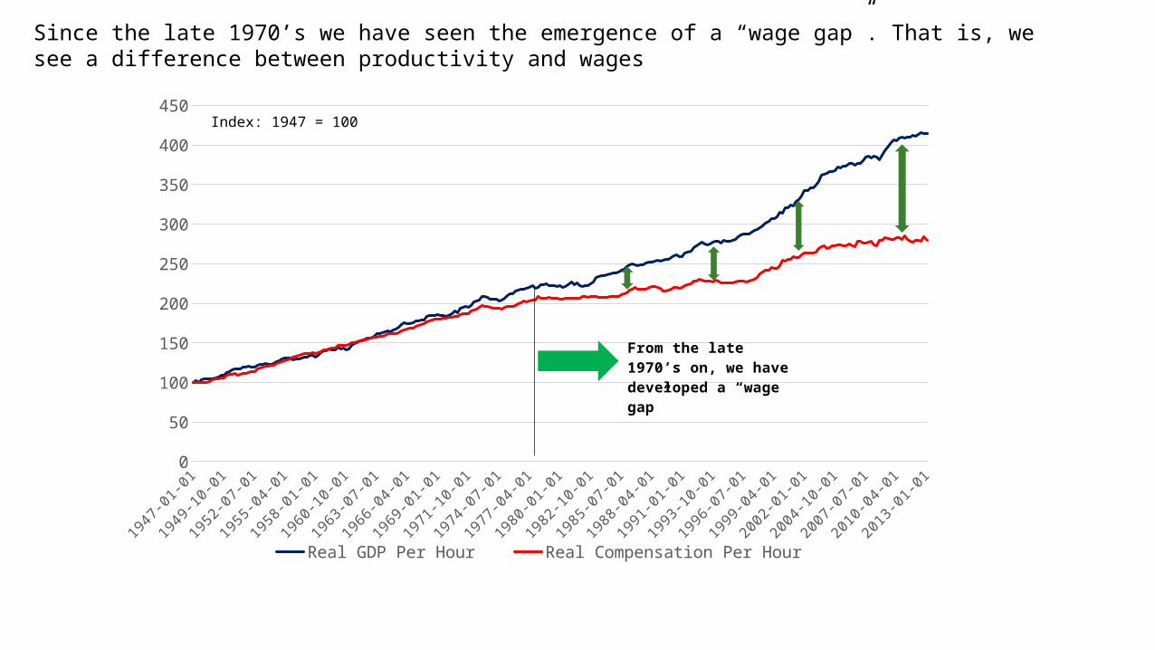
1947 1957 1967 1977 1987 1997 20070
50
100
150
200
250
300
350
400
450
Real GDP Per Hour Real Compensation Per Hour
From the late 1970’s on, we have developed a “wage gap”
Index: 1947 = 100
Since the late 1970’s we have seen the emergence of a “wage gap”. That is, we see a difference between productivity and wages

1964 1969 1974 1979 1984 1989 1994 1999 2004 2009 201430.0
31.0
32.0
33.0
34.0
35.0
36.0
37.0
38.0
39.0
40.0
Average Weekly Hours in the US
Current33.7hrs./wk.
196438.2hrs./wk.
12.5%

1984 1989 1994 1999 2004 200946000
48000
50000
52000
54000
56000
58000
$57,000
Real Median Household Income in the US (2013 Dollars)
Current (2013)$52,000
January 1999 $57,000
January 1989 $53,000
10% Decline

GDP
Time
Trend (Average growth)
The business cycle is a repeated pattern of recessions followed by recoveries
Recession (Below Trend Growth)
Recovery (Above Trend Growth)
Peak
Trough
Peak
Recall, that we are interested in understanding the business cycle…

After removing the long term trend, we end up with a series that looks like this (% deviation from trend)
% Deviation From Trend
Time
0
Trough
Peak Peak
Recession
GDP
Recovery
Peak
Trough
Indu
stria
l Pro
ducti
on (%
Dev
iatio
n fr
om T
rend
)
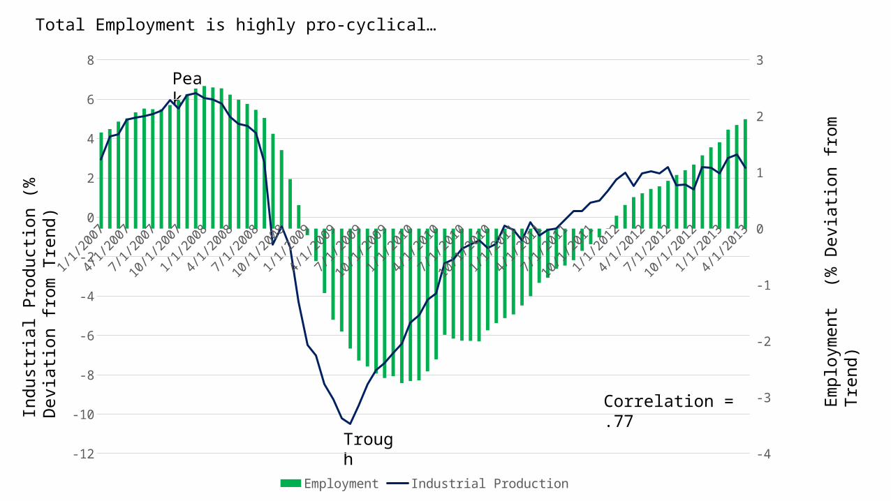
Correlation = .77
1/1/2007 1/1/2009 1/1/2011 1/1/2013
-12
-10
-8
-6
-4
-2
0
2
4
6
8
-4
-3
-2
-1
0
1
2
3
Employment Industrial Production
Empl
oym
ent
(% D
evia
tion
from
Tre
nd)
Total Employment is highly pro-cyclical…

2007-01-01 2009-01-01 2011-01-01 2013-01-01
-4
-3
-2
-1
0
1
2
3
Real Wages Real GDP
Trough
Peak
Dev
iatio
n fr
om T
rend
Correlation = .12
Real wages are pro-cyclical….barely!

At some point in time, you have a fixed number of trees (Capital) and workers
Those workers/capital combine with productivity to produce apples (output)
OR
Those apples are allocated either towards consumption or investment (planting them to grow new trees)
, ,GDP F A K LGDP C I
L
w
p SL
DL
*L
*w
p
For a given capital stock and productivity level, labor markets determine total employment
Recall the apple orchard story….

Labor Markets
L
Total employment (total hours worked)
w
p
Real wages
SLHouseholds choose how much to work
Businesses choose how many hours to hire
DL*L
Equilibrium employment
*w
p
Equilibrium real wage

Labor Markets
L
w
p SL
DL*L
*w
p
Recall that Output = Income
Labor Income + Capital Income
*, ,GDP F A K L
Predetermined
Employment will determine total production (GDP)
=
*
**w
Lp
= Labor Income
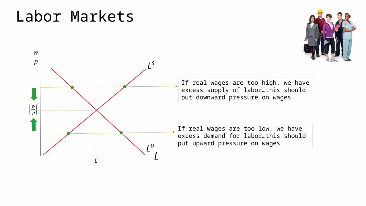
Labor Markets
L
w
p SL
DL*L
*w
p
If real wages are too high, we have excess supply of labor…this should put downward pressure on wages
If real wages are too low, we have excess demand for labor…this should put upward pressure on wages

Labor Demand
L
w
p
DL
We assume that labor markets are populated by perfectly competitive firms
Why is this important?
These firms are making hiring decisions to maximize profits.
Y kProfit p Y wL p r K
),,( LKAFY
Capital costs (fixed)
Nominal Wage rate (fixed)
Price of Output (fixed)

, ,Y F A K L
Y
L
These firms use a production process that exhibits diminishing marginal productivity – that is as labor rises, its contribution to production of output shrinks
1L 2L 3L
So, absent productivity growth, increasing labor will lower the marginal product of labor
YMPL
L
1MPL
2MPL
3MPL
L
Y
LY
L Y

, ,Y F A K L
Y
L1L 2L 3L
1 4MPL
2 2MPL
3 .5MPL
1L
1L
2Y 1L .5Y
MPL
These firms use a production process that exhibits diminishing marginal productivity – that is as labor rises, its contribution to production of output shrinks
L
4Y
1L 2L 3L
MPL
4
2
.5
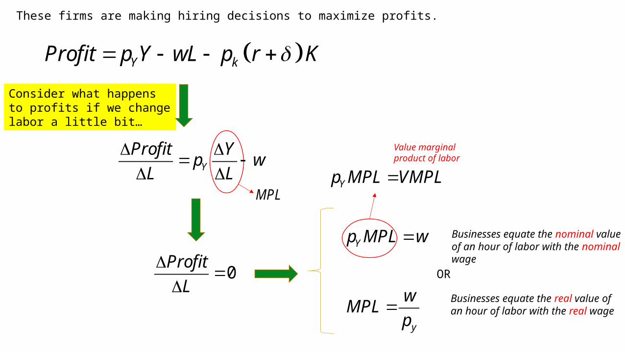
These firms are making hiring decisions to maximize profits.
Y
Profit Yp w
L L
Y kProfit p Y wL p r K
Consider what happens to profits if we change labor a little bit…
MPL
0Profit
L
Yp MPL w
y
wMPL
p
Yp MPL VMPL
Value marginal product of labor
Businesses equate the nominal value of an hour of labor with the nominal wage
Businesses equate the real value of an hour of labor with the real wage
OR

L
MPL
MPL
y
w
p
*LL
Profit
*L
y
wMPL
p
y
wMPL
p
y
wMPL
p
Profits are Decreasing
Profits are increasing
Profits are constant (maximized)
1L 1L2L 2L
Profits are maximized when benefits and costs are equated at the margin!

L
MPL
MPL
L
w
p
DL
1
w
p
2
w
p
1
w
p
2
w
p
1L 2L1L 2L
As wages fall, the marginal cost of labor for businesses drops. This allows them to profitably expand their workforces – even in the light of diminishing marginal returns to labor.
So, these perfectly competitive businesses observe a real wage and make a profit maximizing decision of how much labor to hire. Those decisions are recorded in labor demand.

, ,Y F A K L
Y
L1L 2L 3L
1L
1L
3Y
1L 1Y
MPL
Suppose the economy experiences an increase in productivity….
L
6Y
1L 2L 3L
MPL
4
2
.5
1
3
6
This increase in productivity not only raises total output for every hour of labor worked, but increases the marginal product of every hour worked

L
MPL
MPL
L
w
p
DL
1
w
p
1
w
p
1L1L
As events occur that influence the value of labor at the margin these businesses re-evaluate their hiring decisions and adjust their workforce accordingly.
This increase in labor productivity increases labor demanded.

Labor Supply
L
w
pSL
Just as businesses make decisions to maximize profits, we make decisions to maximize our utility
Make ourselves as happy as possible
( , )U U C Time L
We only have a couple requirements for utility functions• Utility is increasing in consumption (i.e. we like to buy things!)• Utility is decreasing in labor (we don’t like to work)• Utility exhibits diminishing marginal utility (the more we have of
anything, the less it is worth to us at the margin)
Leisure timeReal Consumption
Total Utility (Happiness)

Let’s suppose the following…you have a job opportunity that pays $12 an hour. You can work as much or as little as you want. Further, assume that the only good to buy is pizza and a pizza costs $10. Finally, assume that you have scholarship that pays you $20 per week (you don’t have to work for the stipend). How many hours would you choose to work?
Hours available: 24 hrs./day- 8 hrs./day (sleep) 16 hrs./day*7 days/wk. = 112 hrs.
Nominal Wage = $12/hr.Price (Pizza) = $10Real Wage = 1.2 Pizza/Hr.
Non-Labor Income = $20/wk.Real Non-Labor Income = 2 Pizza/wk.
112Leisure L
( )Pizza C
112
No Work• Labor Income = $0• Stipend = $20• Total Income = $20• Pizzas Bought = 2
2
0
Work 30 Hrs.• Labor Income = $360• Stipend = $20• Total Income = $380• Pizzas Bought = 38
136.4
Work 112 Hrs.• Labor Income = $1,344• Stipend = $20• Total Income = $1,364• Pizzas Bought = 136.4
82
38
136.4 381.2
82 0Slope
38 21.2
112 82Slope
(Real Wage)
(Real Wage)

What you choose to do depends on your preferences!
( , )U U C Time L Leisure timeReal
Consumption
Total Utility (Happiness)
1 hour of leisure. What's that leisure worth to you?
If you work 1 additional hour, what is it cost you?
If you work 1 additional hour, what do you gain?
Value of an hour of leisure
LeisureMU
1.2 pizzas (the real wage). How much are those pizzas worth to you?
ConsumptionMUy
w
p
Number of pizzas you get per hour of work (real wage)
Value of a pizza

Just like with businesses, when we maximize our utility (happiness), we equate costs and benefits at the margin)
ConsumptionMUy
w
p
LeisureMU
Benefits of working Cost of working
=
Let’s rewrite this…
Leisure
y Consumption
MUwMRS
p MU
Marginal Rate of Substitution
Marginal Rate of substitution measures the value of leisure in terms of consumption
. .
Leisure
Consumption
UtilityMU PizzasHr of Leisure
MRSUtilityMU Hr of LeisurePizza

( , )U U C Time L Leisure timeReal
Consumption
Total Utility (Happiness)
We only have a couple requirements for utility functions• Utility is increasing in consumption (i.e. we like to buy things!)• Utility is decreasing in labor (we don’t like to work)• Utility exhibits diminishing marginal utility (the more we have of
anything, the less it is worth to us at the margin)
L
MRSMRS
1MRS
1L 2L
Leisure
Consumption
MUMRS
MU
2MRS • High marginal utility of leisure• Low Marginal Utility of Consumption• High MRS
As you work more, consumption increases and the marginal utility of that consumption falls
As you work more, leisure falls and the marginal utility of that leisure increases
• Low marginal utility of leisure• High Marginal Utility of Consumption• Low MRS

L
MRSMRS
1.2w
p
* 40L
112Leisure L
( )Pizza C
112
2
0
136.4
50
136.4 21.2
112 0Slope
(Real Wage)
72
y
wMRS
p
y
wMRS
p
Work 40 Hrs.• Labor Income = $480• Stipend = $20• Total Income = $500• Pizzas Bought = 50
Utility is decreasingUtility is increasing
y
wMRS
p
y
wMRS
p
Of all the affordable choices, the one that equates costs and benefits at the margin is the best choice!
112Leisure L
( )Pizza C
112
2
0
136.4
50
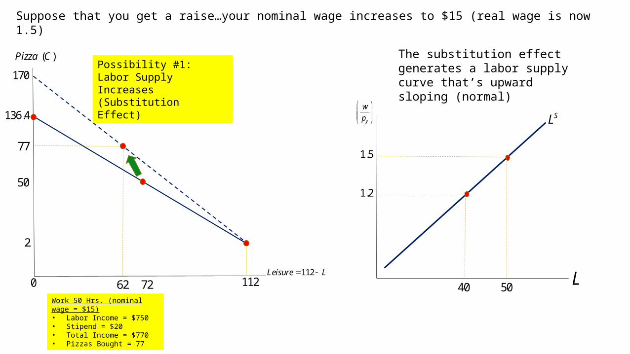
72Work 50 Hrs. (nominal wage = $15)• Labor Income = $750• Stipend = $20• Total Income = $770• Pizzas Bought = 77
Suppose that you get a raise…your nominal wage increases to $15 (real wage is now 1.5)
170
L
y
w
p
SL
1.2
40
1.5
62 50
77
Possibility #1: Labor Supply Increases (Substitution Effect)
The substitution effect generates a labor supply curve that’s upward sloping (normal)

112Leisure L
( )Pizza C
112
2
0
136.4
50
72
Work 35 Hrs. (nominal wage = $15)• Labor Income = $525• Stipend = $20• Total Income = $545• Pizzas Bought = 54.5
Suppose that you get a raise…you nominal wage increases to $15 (real wage is now 1.5)
170
L
y
w
p
SL
1.2
40
1.5
77 35
77
Possibility #2: Labor Supply decreases (Income Effect)
The income effect generates a labor supply curve that’s downward sloping (weird)
54.5

L
y
w
p
SL
1.2
40
1.5
35L
y
w
p
SL
1.2
40
1.5
50
So, which is it? Possibility #2: Labor Supply decreases (Income Effect)
We usually assume the income effect dominates!
Possibility #1: Labor Supply Increases (Substitution Effect)
OR

112Leisure L
( )Pizza C
112
2
0
136.4
50
72
154.4
82
56
Suppose that your stipend increases to $200/wk. (Wage rate is still $12)
20
L
y
w
p
SL
1.2
40
1.5
30
This is a pure income effect (the wage didn’t change, so there is no substitution effect)
Labor supplied declines (labor supply shifts left)
Work 30Hrs. (nominal wage = $12)• Labor Income = $360• Stipend = $200• Total Income = $560• Pizzas Bought = 56

Labor Markets – Equilibrium
L
w
pSL
Households choose how much to work
Businesses choose how many hours to hire
DL*L
*w
p
Real Wage
Total Hours
Now, we just need to put the pieces together and solve for an equilibrium wage

Labor Markets – Long Run dynamics
L
w
p SL
DL*L
*w
p
Long term productivity growth raises the value of labor at the margin – increasing labor demand
As our incomes rise, the value of our leisure time increases – labor supply drops
Over the long term, real wages and employment rise

Labor Markets – Business cycle dynamics
L
w
p SL
DL*L
*w
p
During economic expansions, labor productivity is above trend…the pushes labor demand up – employment and real wages rise above trend
During recessions, labor productivity is below trend…this pushes labor demand down – employment and real wages fall below trend An increase (decrease) in employment raises
(decreases) production.
*, ,GDP F A K L

% Deviation From Trend
Time
0Trough
Peak Peak
Recession
GDP
Recovery
During recessions, productivity declines. Labor demand falls – employment and real wages fall.
w
p
L
sL
DL
w
p
L
sL
DL
During recoveries, productivity increases. Labor demand rises – employment and real wages increase.
Real Wage Employment Productivity
GDP + + +
Predicted Correlations
Real Wages
Employment
Productivity

Correlations With GDP
The only problem we have is explaining the low correlation between real wages and GDP
Some Suggestions• Are we valuing labor contracts correctly?• Have we calculated real wages correctly?• Do wages actually adjust (most labor contracts are
fixed for extended periods)• Does minimum wage affect this analysis?• Is our story correct?
L
w
p SL
Our story for labor supply says that higher wages increase hours worked
In Theory
Empirically
L
SL
*L
w
p
L
SL
*L
w
p
At the individual level, labor supply is very inelastic
At the macro level, there is labor supply is very elastic
Real Wage Employment Productivity
Actual + (.12)
+(.77)
+ (.67)
Predicted + + +

Example: Oil Price Shocks in the 1970’s
Dol
lars
per
Bar
rel
1973 Arab Oil Embargo
1979 Iranian Revolution
We can think about high oil prices as a negative shock to productivity…remember, we measure GDP as value added and (given that the US imports a lot of oil), high energy prices will lower value added

% D
evia
tion
Fro
m T
rend
Real Compensation (1972 – 1982)
1973 Arab Oil Embargo
1979 Iranian Revolution
w
p
L
sL
DL
w
p
L
sL
DL
The high oil prices lowers the value of labor at the margin…labor demand falls and real wages drop

% D
evia
tion
Fro
m T
rend
Employment (1972 – 1982)
1973 Arab Oil Embargo
1979 Iranian Revolution
w
p
L
sL
DL
w
p
L
sL
DL
The drop in labor demand also lowers the new equilibrium level of employment

% D
evia
tion
Fro
m T
rend
GDP (1972 – 1982)
1973 Arab Oil Embargo
1979 Iranian Revolution
w
p
L
sL
DL
w
p
L
sL
DL
Lower employment will lower total production (GDP)
*, ,GDP F A K L

President Obama has proposed the following:
• Raise the minimum wage from its current level of $7.25/hr. to $10.10/hr. by 2016
• Automatic cost of living adjustments thereafter
Application: The Minimum Wage
What do you think?

$7.25 (2009)


Minimum wages around the world

Adjusting for purchasing power changes the story a little….

Minimum wage laws vary by state….

In 2011, 73.9 million American workers age 16 and over were paid at hourly rates, representing 59.1 percent of all wage and salary workers.
• 16 million hourly workers earn less than the proposed $10.10 per hour• 1.7 million earned exactly the prevailing Federal minimum wage of $7.25 per hour. • About 2.2 million had wages below the minimum ($2.13/hr. is the minimum wage for tipped employees).
Source: Department of Labor

Most minimum wage workers are part time
Source: Department of Labor
0 to 4 hours
5 to 9 hours
10 to 14 hours
15 to 19 hours
20 to 24 hours
25 to 29 hours
30 to 34 hours
35 to 39 hours
40 hours 41 + hours
hours vary
0
2
4
6
8
10
12
14
16
18
20Pe
rcen
t of m
inim
um w
age
wor
kers

12 companies with most minimum-wage workers
Darden Restaurants
DineEquity
Yum Brands

Highest wage retail companies
$13.38/hr
$11.27/hr
$11/hr
$10.20/hr
$9.67/hr
$9.67/hr
$9.48/hr $9.38/hr
$9.32/hr$9.24/hr

Costco's CEO and president, Craig Jelinek, has publicly endorsed raising the federal minimum wage to $10.10 an hour, and he takes that to heart. The company's starting pay is $11.50 per hour, and the average employee wage is $21 per hour, not including overtime.

Microeconomic Argument for minimum wage increase: minimum wage workers are underpaid…but really, we are all underpaid in a competitive market!
p
w
*
p
w
*LL
DL
SL Labor supply ranks us by the value of our free time
Labor demand ranks us by our productivity
The equilibrium wage reflects the productivity/free time of the marginal worker
For the average worker, they are being paid less than they are worth, but more than their time is worth.

Macroeconomic argument for minimum wage increase: Increasing the minimum wage would put more money into the economy, but does it?
• An increase to $10.10 would amount to a $2.85 per hour raise for those currently on minimum wage
• For a 40 hour week, that would amount to $5700 per year• If we assume that all 16 million people affected got the full $5700, that
would be an increase in income of $91.2B• $91.2B represents around .5% of the US economy
However, can this really be an increase in income?
Unless an increase in the minimum wage makes us more productive,
NO!

Microeconomic argument for increasing the minimum wage: We are creating a better distribution of income, but are we?
Case #1: Rise in minimum wage results in increased unemployment
So we have a transfer from one lower income group to another lower income group
Case #2: Rise in minimum wage creates no job loss and business can’t pass the higher costs onto consumers
Now we have a transfer from business owners to minimum wage workers
Case #3: Rise in minimum wage creates no job loss, but businesses can pass the increased cost onto consumers
Now we have a transfer from consumers to minimum wage workers