final capstone report a14-159 frans georges
TRANSCRIPT

University of Technology, Sydney
Faculty of Engineering and Information Technology
DEVELOPMENT OF A COMPUTER PROGRAM FOR PILE AND DEEP FOUNDATION ANALYSIS IN COHESIVE AND COHESIONLESS SOILS
by
Frans Georges
Student Number: 11035401
Project Number: A14-159
Major: Civil Engineering (Structural)
Supervisor: A/Prof Hadi Khabbaz
A 12 Credit Point Project submitted in partial fulfilment of the requirement for the Degree of Bachelor of Engineering
21 November 2014

ii

iii
Statement of Originality
I declare that I am the sole author of this report, that I have not used fragments of
text from other sources without proper acknowledgement; that theories, results
and designs of others that I have incorporated into this report have been
appropriately referenced and all sources of assistance have been acknowledged.
Signed,
Frans Georges

iv
Abstract
This Capstone project is centred on the development of a computer program that aids a user in the design of deep foundations and piles in cohesive and cohesionless soils. This project was completed by Frans Georges in the Autumn and Spring semesters of 2014.
The topic of deep foundations is fundamental in the study of geotechnical engineering, and the idea of developing a program that focuses on this particular area seemed like an excellent idea to focus the Capstone project on. The idea was to develop a piece of software that would be a meaningful contribution to the field of geotechnical engineering, and one that could be expanded upon or used as a benchmark by a future Capstone student.
The program is coded using Visual Basic 6, a very simple yet very powerful tool to build such a program. The focus was to originally build a program that dealt with the axial capacities of pile foundations, but quickly expanded the idea to include lateral capacities of piles also. To ensure the accuracy of the program is of working order, and that it returns acceptable and accurate results, manually calculated examples have been tested and compared, which have been discussed in great detail throughout the report.

v
Acknowledgments
There are many people I would like to extend my thanks and appreciation to, for the help and support they have provided throughout the year whilst I have been working on this project. First and foremost, I would like to express my gratitude to my supervisor for this project, Hadi Khabbaz, for providing the help and ideas throughout the course of the project and guiding me to produce both the report and the program to the best of my ability.
The main source of love and support, from whom I could not have done without through this challenging year would definitely be from my family, close friends, and God, who have guided me every step of the way in order to successfully complete this project and this degree. Their presence, care and motivation are what have helped me get over the finish line.
Finally, I would like to acknowledge my late grandfather, Hanna Sleewa, who passed away on the 5th of June, 2014. He was a very loving and humble man, father and grandfather, and was a central figure during my early childhood. He inspired me to always be the best I could be, and his memory and love will live long in my heart.
This piece of work is dedicated to him.
vi
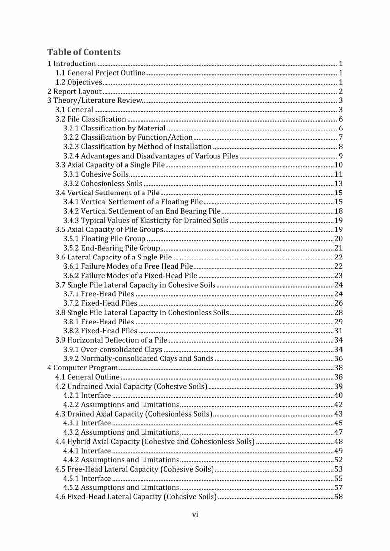
Table of Contents 1 Introduction ................................................................................................................................................. 1
1.1 General Project Outline .................................................................................................................... 1 1.2 Objectives .............................................................................................................................................. 1
2 Report Layout .............................................................................................................................................. 2 3 Theory/Literature Review ...................................................................................................................... 3
3.1 General ................................................................................................................................................... 3 3.2 Pile Classification ............................................................................................................................... 6
3.2.1 Classification by Material ....................................................................................................... 6 3.2.2 Classification by Function/Action ....................................................................................... 7 3.2.3 Classification by Method of Installation ........................................................................... 8 3.2.4 Advantages and Disadvantages of Various Piles ........................................................... 9
3.3 Axial Capacity of a Single Pile ...................................................................................................... 10 3.3.1 Cohesive Soils ............................................................................................................................ 11 3.3.2 Cohesionless Soils ................................................................................................................... 13
3.4 Vertical Settlement of a Pile ......................................................................................................... 15 3.4.1 Vertical Settlement of a Floating Pile ............................................................................... 15 3.4.2 Vertical Settlement of an End Bearing Pile .................................................................... 18 3.4.3 Typical Values of Elasticity for Drained Soils ............................................................... 19
3.5 Axial Capacity of Pile Groups ....................................................................................................... 19 3.5.1 Floating Pile Group ................................................................................................................. 20 3.5.2 End-Bearing Pile Group ......................................................................................................... 21
3.6 Lateral Capacity of a Single Pile .................................................................................................. 22 3.6.1 Failure Modes of a Free Head Pile ..................................................................................... 22 3.6.2 Failure Modes of a Fixed-Head Pile .................................................................................. 23
3.7 Single Pile Lateral Capacity in Cohesive Soils ....................................................................... 24 3.7.1 Free-Head Piles ........................................................................................................................ 24 3.7.2 Fixed-Head Piles ...................................................................................................................... 26
3.8 Single Pile Lateral Capacity in Cohesionless Soils ............................................................... 28 3.8.1 Free-Head Piles ........................................................................................................................ 29 3.8.2 Fixed-Head Piles ...................................................................................................................... 31
3.9 Horizontal Deflection of a Pile .................................................................................................... 34 3.9.1 Over-consolidated Clays ....................................................................................................... 34 3.9.2 Normally-consolidated Clays and Sands ........................................................................ 36
4 Computer Program .................................................................................................................................. 38 4.1 General Outline ................................................................................................................................. 38 4.2 Undrained Axial Capacity (Cohesive Soils) ............................................................................ 39
4.2.1 Interface ...................................................................................................................................... 40 4.2.2 Assumptions and Limitations ............................................................................................. 42
4.3 Drained Axial Capacity (Cohesionless Soils) ......................................................................... 43 4.3.1 Interface ...................................................................................................................................... 45 4.3.2 Assumptions and Limitations ............................................................................................. 47
4.4 Hybrid Axial Capacity (Cohesive and Cohesionless Soils) ............................................... 48 4.4.1 Interface ...................................................................................................................................... 49 4.4.2 Assumptions and Limitations ............................................................................................. 52
4.5 Free-Head Lateral Capacity (Cohesive Soils) ........................................................................ 53 4.5.1 Interface ...................................................................................................................................... 55 4.5.2 Assumptions and Limitations ............................................................................................. 57
4.6 Fixed-Head Lateral Capacity (Cohesive Soils) ...................................................................... 58
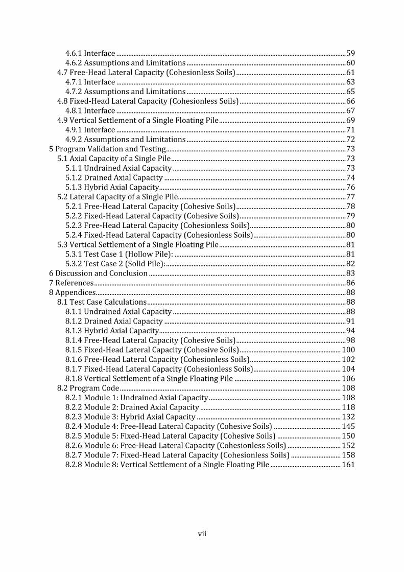
vii
4.6.1 Interface ...................................................................................................................................... 59 4.6.2 Assumptions and Limitations ............................................................................................. 60
4.7 Free-Head Lateral Capacity (Cohesionless Soils) ................................................................ 61 4.7.1 Interface ...................................................................................................................................... 63 4.7.2 Assumptions and Limitations ............................................................................................. 65
4.8 Fixed-Head Lateral Capacity (Cohesionless Soils) .............................................................. 66 4.8.1 Interface ...................................................................................................................................... 67
4.9 Vertical Settlement of a Single Floating Pile .......................................................................... 69 4.9.1 Interface ...................................................................................................................................... 71 4.9.2 Assumptions and Limitations ............................................................................................. 72
5 Program Validation and Testing ......................................................................................................... 73 5.1 Axial Capacity of a Single Pile ...................................................................................................... 73
5.1.1 Undrained Axial Capacity ..................................................................................................... 73 5.1.2 Drained Axial Capacity .......................................................................................................... 74 5.1.3 Hybrid Axial Capacity ............................................................................................................. 76
5.2 Lateral Capacity of a Single Pile .................................................................................................. 77 5.2.1 Free-Head Lateral Capacity (Cohesive Soils) ................................................................ 78 5.2.2 Fixed-Head Lateral Capacity (Cohesive Soils) .............................................................. 79 5.2.3 Free-Head Lateral Capacity (Cohesionless Soils) ........................................................ 80 5.2.4 Fixed-Head Lateral Capacity (Cohesionless Soils) ...................................................... 80
5.3 Vertical Settlement of a Single Floating Pile .......................................................................... 81 5.3.1 Test Case 1 (Hollow Pile): .................................................................................................... 81 5.3.2 Test Case 2 (Solid Pile): ......................................................................................................... 82
6 Discussion and Conclusion ................................................................................................................... 83 7 References ................................................................................................................................................... 86 8 Appendices .................................................................................................................................................. 88
8.1 Test Case Calculations .................................................................................................................... 88 8.1.1 Undrained Axial Capacity ..................................................................................................... 88 8.1.2 Drained Axial Capacity .......................................................................................................... 91 8.1.3 Hybrid Axial Capacity ............................................................................................................. 94 8.1.4 Free-Head Lateral Capacity (Cohesive Soils) ................................................................ 98 8.1.5 Fixed-Head Lateral Capacity (Cohesive Soils) ........................................................... 100 8.1.6 Free-Head Lateral Capacity (Cohesionless Soils) ..................................................... 102 8.1.7 Fixed-Head Lateral Capacity (Cohesionless Soils) ................................................... 104 8.1.8 Vertical Settlement of a Single Floating Pile .............................................................. 106
8.2 Program Code ................................................................................................................................. 108 8.2.1 Module 1: Undrained Axial Capacity ............................................................................. 108 8.2.2 Module 2: Drained Axial Capacity .................................................................................. 118 8.2.3 Module 3: Hybrid Axial Capacity .................................................................................... 132 8.2.4 Module 4: Free-Head Lateral Capacity (Cohesive Soils) ....................................... 145 8.2.5 Module 5: Fixed-Head Lateral Capacity (Cohesive Soils) ..................................... 150 8.2.6 Module 6: Free-Head Lateral Capacity (Cohesionless Soils) ............................... 152 8.2.7 Module 7: Fixed-Head Lateral Capacity (Cohesionless Soils) ............................. 158 8.2.8 Module 8: Vertical Settlement of a Single Floating Pile ......................................... 161

viii
List of Figures Figure 1: Pile used above stiff stratum .................................................................................................. 3
Figure 2: Pile used in highly compressible soil .................................................................................. 4
Figure 3: Pile resisting uplift ..................................................................................................................... 4
Figure 4: Pile resisting lateral loads ....................................................................................................... 4
Figure 5: Pile used in offshore structures............................................................................................. 5
Figure 6: Piles set up under shallow foundation ............................................................................... 5
Figure 7: Pile used in expansive soil ....................................................................................................... 5
Figure 8: Various types of piles ................................................................................................................ 8
Figure 9: Adhesion Reduction Factor Chart ...................................................................................... 12
Figure 10: Settlement Influence Factor Chart ................................................................................... 16
Figure 11: Settlement Correction Factor Chart ................................................................................ 17
Figure 12: Settlement Movement Ratio Chart .................................................................................. 18
Figure 13: Stress distribution in a pile group ................................................................................... 20
Figure 14: Block capacity of a pile group ............................................................................................ 21
Figure 15: Failure Modes for a free-headed pile .............................................................................. 23
Figure 16: Failure Modes for a fixed-headed pile ............................................................................ 23
Figure 17: Soil reaction and bending moments in Failure Mode 1 for a free-head pile in cohesive soil ................................................................................................................................................... 24
Figure 18: Load factor chart for Failure Mode 1, free-headed piles in cohesive soils ....... 24
Figure 19: Soil reaction and bending moments in Failure Mode 2 for a free-head pile in cohesive soil ................................................................................................................................................... 25
Figure 20: Load factor chart for Failure Mode 2, free-headed piles in cohesive soils ....... 25
Figure 21: Soil reaction and bending moments in Failure Mode 1 for a fixed-head pile in cohesive soil ................................................................................................................................................... 26
Figure 22: Soil reaction and bending moments in Failure Mode 2 for a fixed-head pile in cohesive soil ................................................................................................................................................... 27
Figure 23: Soil reaction and bending moments in Failure Mode 3 for a fixed-head pile in cohesive soil ................................................................................................................................................... 28
Figure 24: Soil reaction and bending moments in Failure Mode 1 for a free-head pile in cohesionless soil ........................................................................................................................................... 29
Figure 25: Failure chart for Failure Mode 1 for a free-head pile in cohesionless soil ....... 29
Figure 26: Soil reaction and bending moments in Failure Mode 2 for a free-head pile in cohesionless soil ........................................................................................................................................... 30
Figure 27: Failure chart for Failure Mode 2 for a free-head pile in cohesionless soil ....... 30
Figure 28: Soil reaction and bending moments in Failure Mode 1 for a fixed-head pile in cohesionless soil ........................................................................................................................................... 31
Figure 29: Soil reaction and bending moments in Failure Mode 2 for a fixed-head pile in cohesionless soil ........................................................................................................................................... 32
Figure 30: Soil reaction and bending moments in Failure Mode 3 for a fixed-head pile in cohesionless soil ........................................................................................................................................... 33
Figure 31: Plot of self-determined equations for the adhesion reduction factor ............... 39
Figure 32: Undrained Axial Capacity Module Interface ................................................................ 40
Figure 33: Example Drained Axial Capacity problem .................................................................... 44
Figure 34: Drained Axial Capacity Module Interface ..................................................................... 45
Figure 35: Hybrid Axial Capacity Module Interface ........................................................................ 49
Figure 36: Free-Head Lateral Capacity (Cohesive Soils) Module Interface ........................... 55
Figure 37: Fixed-Head Lateral Capacity (Cohesive Soils) Module Interface ......................... 59
Figure 38: Free-Head Lateral Capacity (Cohesionless Soils) Module Interface................... 63

ix
Figure 39: Fixed-Head Lateral Capacity (Cohesionless Soils) Module Interface ................. 67
Figure 40: Vertical Settlement of a Single Floating Pile Module Interface ............................ 71
Figure 41: Undrained Axial Capacity – Test Case 1 ........................................................................ 73
Figure 42: Undrained Axial Capacity – Test Case 2 ........................................................................ 73
Figure 43: Undrained Axial Capacity – Test Case 3 ........................................................................ 74
Figure 44: Drained Axial Capacity – Test Case 1 .............................................................................. 74
Figure 45: Drained Axial Capacity – Test Case 2 .............................................................................. 75
Figure 46: Drained Axial Capacity – Test Case 3 .............................................................................. 75
Figure 47: Hybrid Axial Capacity – Test Case 1 ................................................................................ 76
Figure 48: Hybrid Axial Capacity – Test Case 2 ................................................................................ 76
Figure 49: Lateral Capacity of a Free-Head Pile ............................................................................... 77
Figure 50: Lateral Capacity of a Fixed-Head Pile ............................................................................. 78
Figure 51: Vertical Settlement of a Single Floating Pile ................................................................ 81
List of Tables Table 1: Advantages and Disadvantages of Different Piles ............................................................ 9
Table 2: Typical Values for friction angles ......................................................................................... 14
Table 3: Various values for F and Nq..................................................................................................... 14
Table 4: Typical values of elasticity for cohesive soils .................................................................. 19
Table 5: Typical values of elasticity for cohesionless soils .......................................................... 19
Table 6: Values for the displacement influence factors in clays ................................................ 35
Table 7: Values for the displacement influence factors in sand ................................................. 37
Table 8: Typical values for Nh .................................................................................................................. 37
Table 9: Undrained Axial Capacity Module Variables .................................................................... 41
Table 10: Drained Axial Capacity Module Variables ...................................................................... 46
Table 11: Hybrid Axial Capacity Module Variables......................................................................... 51
Table 12: Self-determined equations for the Free-Head Lateral Capacity (Cohesive) Module .............................................................................................................................................................. 54
Table 13: Free-Head Lateral Capacity (Cohesive) Module Variables ...................................... 56
Table 14: Fixed-Head Lateral Capacity (Cohesive) Module Variables .................................... 60
Table 15: Self-determined equations for Free-Head Lateral Capacity (Cohesionless) Module .............................................................................................................................................................. 62
Table 16: Free-Head Lateral Capacity (Cohesionless) Module Variables .............................. 64
Table 17: Fixed-Head Lateral Capacity (Cohesionless) Module Variables ............................ 68
Table 18: Self-determined equations for Settlement of a Single Floating Pile Module .... 70
Table 19: Settlement of a Single Floating Pile Module Variables .............................................. 71
x
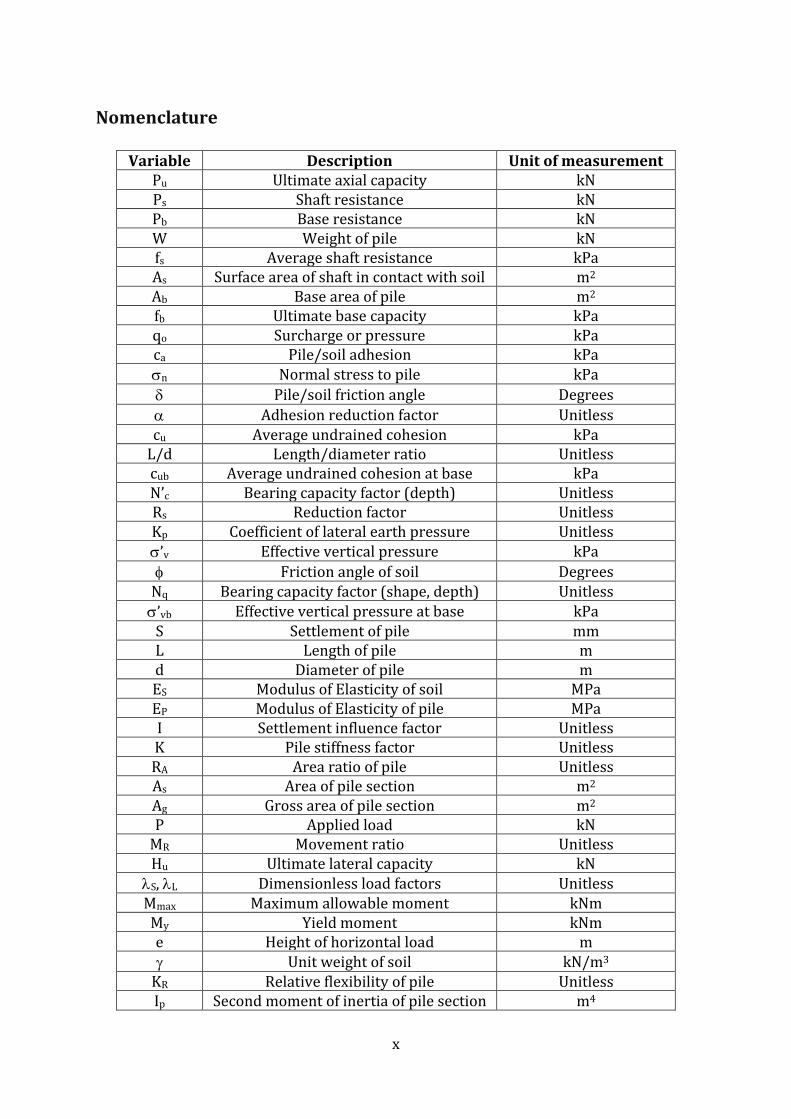
Nomenclature
Variable Description Unit of measurement Pu Ultimate axial capacity kN Ps Shaft resistance kN Pb Base resistance kN W Weight of pile kN fs Average shaft resistance kPa As Surface area of shaft in contact with soil m2 Ab Base area of pile m2 fb Ultimate base capacity kPa qo Surcharge or pressure kPa ca Pile/soil adhesion kPa
n Normal stress to pile kPa
Pile/soil friction angle Degrees
Adhesion reduction factor Unitless cu Average undrained cohesion kPa
L/d Length/diameter ratio Unitless cub Average undrained cohesion at base kPa N’c Bearing capacity factor (depth) Unitless Rs Reduction factor Unitless Kp Coefficient of lateral earth pressure Unitless
’v Effective vertical pressure kPa
Friction angle of soil Degrees Nq Bearing capacity factor (shape, depth) Unitless
’vb Effective vertical pressure at base kPa S Settlement of pile mm L Length of pile m d Diameter of pile m ES Modulus of Elasticity of soil MPa EP Modulus of Elasticity of pile MPa I Settlement influence factor Unitless K Pile stiffness factor Unitless RA Area ratio of pile Unitless As Area of pile section m2 Ag Gross area of pile section m2 P Applied load kN
MR Movement ratio Unitless Hu Ultimate lateral capacity kN
S, L Dimensionless load factors Unitless Mmax Maximum allowable moment kNm My Yield moment kNm e Height of horizontal load m
Unit weight of soil kN/m3 KR Relative flexibility of pile Unitless Ip Second moment of inertia of pile section m4

xi

Capstone Final Report: Frans Georges - 11035401
1
1 Introduction
1.1 General Project Outline
This Capstone project is based in the field of geotechnical engineering, focusing on the development of a computer program for use in the field of deep foundations or piles. Deep foundations are a fundamental topic in the field of civil and geotechnical engineering, being often implemented in many large scale projects around the world. This project will outline the uses, theory and various aspects of piles so as to benefit users at a university level.
1.2 Objectives The objectives of this work are to:
- Locate and research relevant theory relating to deep/pile foundations, focusing mainly on geotechnical engineering textbooks, research papers and lecture notes,
- Identify and summarise the relevant data from these resources into a literature review,
- Utilise appropriate data and theory to create a computer program in Microsoft Visual Basic for solving various problems related to deep foundations/piles,
- Validate the program to ensure its accuracy by comparing it to manually-worked solutions, and
- Identify any areas by which the program could be improved. The program is designed primarily for students who can benefit from it by using it in conjunction with their geotechnical studies. The program on its own will simply provide answers for certain variables and the final required outcome, useful as a check with a manually-worked solution. The program is designed in order to have separate sections all accessible from the main menu; ranging from axial capacities of single piles in a cohesive, cohesionless or a hybrid stratum, lateral capacities of single piles in either a cohesive or cohesionless soil and the vertical settlement of a single pile. As mentioned, this program is not designed to replace worked solutions for the problems it is designed to solve, but rather a cross-checking tool that can help students in solving problems within the topics in the program.
Capstone Final Report: Frans Georges - 11035401
2
2 Report Layout The report follows a specific format, divided up into five specific sections; Theory/Literature Review, Design of the Computer Program, Result Validation, Conclusions and Appendices. A summary of each section is outlined below: Theory/Literature Review – contains details and the theory behind the subject of piles and deep foundations. Understanding the theory described in this section is vital to build a program that can successfully solve the required problem without any issues of its own. Information and data/figures from journal articles and various research papers are also included in this section. Design of the Computer Program – A detailed look into the program designed in Microsoft Visual Basic, including a step-by-step look into each module. Any assumptions and limitations to any module will be listed in this section. Result Validation – A brief look at the accuracy of the computer program against manually-worked solutions. Each module will have a number of test cases considering the number of possible test cases. Detailed worked solutions for each test case will be included in the Appendices. Discussion and Conclusion – A reflection on the project as a whole, and what measures can be taken in order for a more effective and efficient approach for a similar project in the future. Appendices – A detailed look into the validation of results for each test case with fully worked solutions, and a full transcript of the code behind each module of the program.

Capstone Final Report: Frans Georges - 11035401
3
3 Theory/Literature Review
3.1 General
Piles are deep foundations which help transfer the load of very large structures through relatively weaker soil layers into stronger and denser soil or rock layers. Piles are utilised when the soil beneath the surface has insufficient bearing capacity to withstand the load of the large structure, or when the settlement of a shallow foundation within the specific soil is deemed to be too excessive. They can also be used to resist uplift loading, lateral loading and also to support shallow or mat foundations to lessen the settlement of such foundations. Piles can support the applied load through two different methods; by end bearing or by friction/adhesion developed along the length of the pile shaft, or both cases simultaneously. Generally, piles extend to a depth of three metres below ground level. There are several methods to installing of a pile foundation, including:
- Driving - Drilling - Jacking - Vibrating - Casting - Screwing
The appropriate method of installation is utilised relevant to the specific situation or requirement of the pile foundation. Piles can also be grouped together in relatively close proximity in order to form a pile group, usually grouped together by a large pile cap. Pile groups are usually designed to carry extremely large loads, and the pile cap assists in helping transfer the large load through to each pile. Pile foundations are much more expensive to lay than shallow foundations, however, they have much more capability than their shallow counterparts, such as in the uses below:
Used when a stiff layer of soil or rock exists below the softer soil layer above. This then provides an economical solution, as the loads can be directly transferred to the stiff layer below. Figure 1: Pile used above stiff stratum

Capstone Final Report: Frans Georges - 11035401
4
This method gradually transfers the load from the superstructure above via pile-soil friction. This is required when the upper soil layer is highly compressible, therefore being too weak to withstand the loads of the superstructure above.
This method is utilised to resist any uplift in the upper soil layer. Uplift results from loads such as wind loads, the piles being used as machine foundations or utilising the piles as tension members in the soil layers.
Piles can be used to resist horizontal or lateral loads as well as vertical or longitudinal loading. Piles can resist and transfer horizontal loads much better than shallow foundations due to their extended depth under the surface. Horizontal loads are as a result of wind loads, earthquake loads or loads induced from the structure governing the pile, such as bridge footings and abutments.
Figure 2: Pile used in highly compressible soil
Figure 3: Pile resisting uplift
Figure 4: Pile resisting lateral loads

Capstone Final Report: Frans Georges - 11035401
5
This pile setup consists of a group of piles governed by a large cap, being used in an offshore structure where the upmost layer is subject to heavy erosion.
This method involves a group of piles setup below a shallow foundation near an area that is expected to be excavated, where there would be large ground movements and settlements.
In this situation, piles are used instead of shallow foundations due to the swelling and excessive movement from the upper layer expansive or collapsible soils.
Figure 5: Pile used in offshore structures
Figure 6: Piles set up under shallow foundation
Figure 7: Pile used in expansive soil

Capstone Final Report: Frans Georges - 11035401
6
3.2 Pile Classification
3.2.1 Classification by Material
Piles can be classified on their material and composition:
- Timber piles; often constructed from timber of very good quality, and very
useful due to their relatively low cost. Length of timber piles vary, but are usually 10 to 15 metres in length. Longer timber piles require to be spliced for effectiveness. Timber piles range from being 30 to 40 centimetres in diameter and usually perform best in completely dry or saturated conditions. Partially saturated conditions tend to reduce the life of timber piles, unless extra measures are taken, which may not be economically viable in some situations. Timber piles can usually sustain a maximum design load of approximately 250kN.
- Steel piles; usually rolled sections such as H-beams, I-beams, circular or rectangular hollow sections. Typical lengths range from 15 to 60 metres and are not as limited as other types of piles. Other steel piles include hollow segmented piles and sheet piles, which are usually used for the retention of water. Steel piles are usually subject to handling large loads usually in the range of 1000kN or more.
- Concrete piles; can be either one of precast or cast-in-situ. Precast piles are assembled and cast off site, thus requiring space for the casting and storage, extended curing times and heavy machinery for the handling and delivering of the piles. Cast-in-situ piles are cast on site through pre-excavation, which eliminates any damage or vibrations that may affect precast piles through the handling and delivering process.
- Composite piles; usually consist of being a hybrid of concrete and timber pile or a concrete and steel pile. Utilised in areas where the upper section of the pile is above the water table. Composite piles can withstand far greater loads, particularly concrete and steel tiles, due to their combined strengths, however, are usually a very costly option.

Capstone Final Report: Frans Georges - 11035401
7
3.2.2 Classification by Function/Action
Piles can be classified based on their function or action and transmission of loads:
- End-bearing piles; transfers loads through the pile tip to a required layer of soil/rock, usually bypassing the softer layers of soil and water. The shaft of the pile has minimal input to their resistance and thus shaft resistance is deemed negligible during design.
- Floating piles; transfers loads via skin friction along the surface area of the
pile and reactions developed on their base to a required depth to a certain layer of soil/rock. Both shaft resistance and end-bearing resistance are vital in design, however, base resistance offers negligible contribution and is not considered during design.
- Tension/Uplift piles; allows the anchorage of structures that are exposed to uplift forces due to hydrostatic pressures or overturning moments as a result of lateral forces.
- Compaction piles; utilised for the compaction of loose soils to increase
bearing capacity of the weaker soil. As the pile itself is not required to carry any load, the material is not as important, and can actually be created by sand.
- Anchor piles; provides anchorage from lateral forces from water or sheet-piling.
- Fender piles; provides protection for water-front structures.
- Sheet piles; provides prevention of seepage and uplift in hydraulic structures.
- Batter piles; utilised to resist lateral and inclined forces in water front
structures.

Capstone Final Report: Frans Georges - 11035401
8
3.2.3 Classification by Method of Installation
Piles can be classified based on their method of installation:
- Driven piles; piles can be driven position either vertically or at inclined at an angle (piles driven at an angle are usually considered as ‘batter’ or ‘raking’ piles). Piles suited to being driven into position are usually made from timber, steel, or precast concrete.
- Cast-in-situ piles; only possible with concrete or grout, deep holes are
drilled in the ground to the required length of the pile. The hole is then filled with concrete or grout to create the pile. Steel reinforcement may be used if necessary.
- Driven and cast-in-situ; this combines both of the aforementioned methods
of installation. This method usually involves a liner (either temporary or permanent) being driven into place and the resulting void being filled with either concrete or grout to complete the pile. If the liners are temporary, they are extracted at the pouring process.
The table on the following page summarises the different types of piles used in construction along with their advantages and disadvantages among other useful information.
Figure 8: Various types of piles

Capstone Final Report: Frans Georges - 11035401
9
3.2.4 Advantages and Disadvantages of Various Piles
Table 1: Advantages and Disadvantages of Different Piles

Capstone Final Report: Frans Georges - 11035401
10
3.3 Axial Capacity of a Single Pile
Through the process of static analysis, it is possible to determine the ultimate axial capacity of a lone pile. The ultimate axial capacity of a single pile, Pu, in compression loading, can be determined with the following formula:
Where; Ps = Shaft resistance Pb = Base resistance W = Weight of pile Shaft Resistance, Ps, can be determined by:
Where; fs = Average shaft resistance (kPa) As = Surface area of the shaft in contact with soil (m2) Base resistance, Pb, can be determined by:
Where; Ab = Area of base of pile (m2) fb = Base ultimate capacity (kPa) qo = Surcharge/Pressure at base level (kPa) Thus, the initial formula for ultimate axial capacity would read;
However, it is assumed that Abqo is approximately = W, therefore simplifying the equation to:

Capstone Final Report: Frans Georges - 11035401
11
The value for fs is calculated using the Mohr-Coulomb failure criterion and the value for fb can be derived from relevant bearing capacity equations, similar to that of shallow foundations. The values used to determine these values vary with regards to soil and pile type, and method utilised for the installation of the relevant pile. When performing these analyses, conventional rules of soil mechanics apply. This being, using total stresses when performing an undrained analysis for a cohesive soil and using effective stresses when performing a drained analysis for a cohesionless soil. Cohesive and cohesionless soils both utilise differing methods to determine the ultimate axial capacity of piles, and piles that are in layers of soil that are both cohesive and cohesionless use a combination of both methods in order to determine ultimate capacity.
3.3.1 Cohesive Soils
Cohesive soils, such as clay, exhibit their lowest strength when fully saturated and are put under fast undrained loading. Hence, in order to determine the ultimate capacity, an undrained analysis is required. Some assumptions to be made when performing an undrained analysis are that the friction angle , is assumed to be zero and that the shearing strength of the soil is directly correlated to the undrained cohesion, cu. Generally, the average shaft resistance, fs, can be determined by:
Where; ca = Pile/soil adhesion (kPa) n = Normal stress to the pile (kPa) = Pile/soil friction angle However, for cohesive soils in an undrained analysis, fs is simplified to:
The term ca is simply the adhesion between the soil and the pile. To determine ca, the following formula must be used:
Where; = Adhesion reduction factor cu = Avarage undrained shear strength of soil (kPa)

Capstone Final Report: Frans Georges - 11035401
12
The adhesion reduction factor is determined by utilising the following chart, using the undrained shear strength of the relevant soil:
For slender piles, i.e. piles that have a length to diameter ratio (L/d) of greater than 50, must have their respective Ps value multiplied by a reduction factor, Rs (Semple & Rigden, 1984). Rs is dependant on the length to diameter ratio of the pile. Possible values for Rs are:
The base ultimate capacity, fb, for a cohesive soil, is determined by:
Where; cub = Average undrained shear strength of soil at base of pile (kPa) N’c = Bearing capacity factor including depth factor
Figure 9: Adhesion Reduction Factor Chart

Capstone Final Report: Frans Georges - 11035401
13
The bearing capacity factor, N’c, similar to the reduction factor Rs, is dependant on the length to diameter ratio of the pile. Possible values for N’c are:
The calculated value for fb is then multiplied by the area of the base of the pile to determine the total base resistance of the pile. Therefore, for a cohesive soil, the ultimate undrained capacity is determined as:
3.3.2 Cohesionless Soils
Cohesionless soils account for the rough and granular soils, such as sand, which possess little to no cohesion and very high friction. Thus, to determine the ultimate capacity of a pile in a cohesionless soil, a drained analysis is required. A drained analysis utilises the drained strength values of c’ and ’ and fully depends on the use of effective stresses rather than total stresses. Assumptions in this form of analysis include the soil having zero cohesion, i.e. c’ = 0. Hence the shaft friction is totally dependant on the soil-pile friction angle, , and the effective horizontal pressures acting on the pile due to the soil, ’n. Thus, to calculate fs for a cohesionless soil, the following relationship is used:
The effective normal pressures equal to the effective horizontal pressures, and thus are calculated by multiplying the corresponding effective vertical pressures, ’v, at the required point by K, the coefficient of lateral earth pressure. The value of the friction angle between the soil and the pile, , differs depending on the type of soil and the method used to install the pile itself. The value of the friction angle between the soil and pile is usually less than the internal friction angle of the soil, . The following table outlines typical values for and .

Capstone Final Report: Frans Georges - 11035401
14
Interface Materials
Driven Piles Sand/rough concrete 1.0 Sand/smooth concrete 0.8 – 1.0 Sand/rough steel 0.7 – 0.9 Sand/smooth steel 0.5 – 0.7 Sand/timber 0.8 – 0.9 Bored Piles 1.0 However, for simplification of calculation, the term Ktan in the calculation of fs can be represented by the single variable F, the coefficient of shaft friction. Therefore, the calculation of fs is basically simplified to:
The following table below outlines the various values that F can represent, depending on the soil consistency, relative density and installation method of the pile. The table also summarises the possible values for Nq, the bearing capacity factor (for shape and depth factors), which is utilised in the calculation of fb for cohesionless soils.
Soil Consistency
Relative Density
F = Ktan Nq
Driven Bored/cast
in-situ Driven
Bored/cast in-situ
Loose 0.2 – 0.4 0.8 0.3 60 25 Medium 0.4 – 0.75 1.0 0.5 100 60
Dense 0.75 – 0.9 1.5 0.7 180 100 The value for fs should also be modified by the slenderness reduction factor, Rs, if the pile is a slender pile, i.e. L/d > 50, as it was in the undrained analysis for cohesive soils. The base ultimate capacity factor, fb, for a cohesionless soil, is determined by:
Where; ’vb = vertical effective stress at base of pile (kPa) Nq = Bearing capacity factor for depth and shape The calculated value for fb is then multiplied by the area of the base of the pile to determine the total base resistance of the pile.
Table 2: Typical Values for friction angles
Table 3: Various values for F and Nq

Capstone Final Report: Frans Georges - 11035401
15
Therefore, for a cohesive soil, the ultimate undrained capacity is determined as:
3.4 Vertical Settlement of a Pile
For the calculation of the settlement of a single pile, the theory of elasticity must be implemented. Results are approximate, but the method is a lot more feasible and economical to carry out than the more accurate method of load testing. It is understood that roughly 80% of settlement is understood to be elastic with the remaining 20% often due to consolidation.
3.4.1 Vertical Settlement of a Floating Pile
The settlement, S, of a single floating pile is obtained through the following relationship:
Where; P = Load applied to pile (kN) L = Length of pile (m) Es = Modulus of Elasticity of soil foundation (MPa) I = Influence factor The influence factor, I, can be obtained using the chart on the following page.

Capstone Final Report: Frans Georges - 11035401
16
To effectively use this chart, the pile stiffness factor, K, is required, which is cross-referenced with the L/d ratio.
K is given as:
Where: Ep = Young’s Modulus of Pile Es = Young’s Modulus of Soil RA = Area ratio of pile
Figure 10: Settlement Influence Factor Chart

Capstone Final Report: Frans Georges - 11035401
17
RA is given as:
Where: As = Area of pile section Ag = Gross area Therefore, solid piles have an RA value of 1, while hollow piles have an RA value of less than 1. If a rigid base exists under the embedment of the pile, the total settlement is modified by a correction factor, Rh. The correction factor can be determined by using the chart shown below.
Figure 11: Settlement Correction Factor Chart
Capstone Final Report: Frans Georges - 11035401
18
3.4.2 Vertical Settlement of an End Bearing Pile
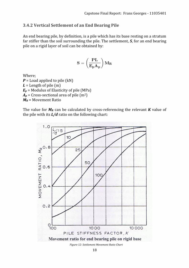
An end bearing pile, by definition, is a pile which has its base resting on a stratum far stiffer than the soil surrounding the pile. The settlement, S, for an end bearing pile on a rigid layer of soil can be obtained by:
Where; P = Load applied to pile (kN) L = Length of pile (m) Ep = Modulus of Elasticity of pile (MPa) Ap = Cross-sectional area of pile (m2) MR = Movement Ratio The value for MR can be calculated by cross-referencing the relevant K value of the pile with its L/d ratio on the following chart:
Figure 12: Settlement Movement Ratio Chart
Capstone Final Report: Frans Georges - 11035401
19
3.4.3 Typical Values of Elasticity for Drained Soils
When no data is provided for the calculation of settlement, the following values can be used depending on the situation at hand, for drained soils.
Cohesive Soil Undrained Cohesion,
cu (kPa) Young’s Modulus, Es (MPa)
Bored/cast in-situ Driven 35 3.8 8.5 70 8.5 25.0
105 22.0 35.0 140 70.0 35.0
Cohesionless Soil Soil Consistency Young’s Modulus, E’s (MPa)
Loose Sand 42 Medium Sand 70
Dense Sand 90 Medium Gravel 200
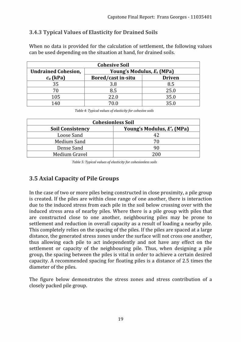
3.5 Axial Capacity of Pile Groups
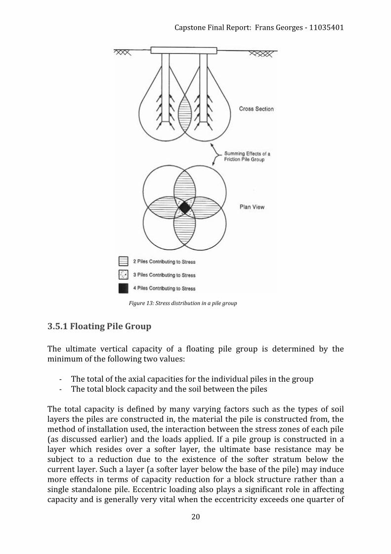
In the case of two or more piles being constructed in close proximity, a pile group is created. If the piles are within close range of one another, there is interaction due to the induced stress from each pile in the soil below crossing over with the induced stress area of nearby piles. Where there is a pile group with piles that are constructed close to one another, neighbouring piles may be prone to settlement and reduction in overall capacity as a result of loading a nearby pile. This completely relies on the spacing of the piles. If the piles are spaced at a large distance, the generated stress zones under the surface will not cross one another, thus allowing each pile to act independently and not have any effect on the settlement or capacity of the neighbouring pile. Thus, when designing a pile group, the spacing between the piles is vital in order to achieve a certain desired capacity. A recommended spacing for floating piles is a distance of 2.5 times the diameter of the piles. The figure below demonstrates the stress zones and stress contribution of a closely packed pile group.
Table 4: Typical values of elasticity for cohesive soils
Table 5: Typical values of elasticity for cohesionless soils
Capstone Final Report: Frans Georges - 11035401
20
3.5.1 Floating Pile Group
The ultimate vertical capacity of a floating pile group is determined by the minimum of the following two values:
- The total of the axial capacities for the individual piles in the group - The total block capacity and the soil between the piles
The total capacity is defined by many varying factors such as the types of soil layers the piles are constructed in, the material the pile is constructed from, the method of installation used, the interaction between the stress zones of each pile (as discussed earlier) and the loads applied. If a pile group is constructed in a layer which resides over a softer layer, the ultimate base resistance may be subject to a reduction due to the existence of the softer stratum below the current layer. Such a layer (a softer layer below the base of the pile) may induce more effects in terms of capacity reduction for a block structure rather than a single standalone pile. Eccentric loading also plays a significant role in affecting capacity and is generally very vital when the eccentricity exceeds one quarter of
Figure 13: Stress distribution in a pile group

Capstone Final Report: Frans Georges - 11035401
21
the width of the pile group. If a pile cap is installed on top of the pile group, the total capacity of each pile in the group is increased due to the extra resistance provided by the pile cap. The increased resistance from the pile cap is due to the net area of the pile cap which induces its own capacity. This net area is the gross area of the pile cap minus the total areas of the cross-sections of the existing piles within the pile group.
3.5.2 End-Bearing Pile Group
In the case of a group of piles constructed over a stiffer stratum such as rock or dense sand or gravel, in comparison to the surrounding soil, the ultimate capacity of the pile group is simply taken as the sum of the ultimate axial capacities of each pile within the group. The typical spacing for piles within an end-bearing pile group is usually more than twice the diameter of the piles.
Figure 14: Block capacity of a pile group

Capstone Final Report: Frans Georges - 11035401
22
3.6 Lateral Capacity of a Single Pile
For single piles, the lateral capacity is just as important to determine as the axial capacity as they are designed in order to sustain fairly large horizontal loads. However, the lateral capacity can be limited by other factors, such as the shearing capacity of the soil the pile is installed in, the pile’s own structural capacity, or through excessive lateral deformation of the pile. The design steps in order to design a pile for its lateral capacity depend on a number of factors such as the type of soil, the possible failure modes of the pile (discussed later on) and the pile cap rigidity. If the pile is not restricted from rotation at the pile head, the pile is known as a free-head pile. If, however, a pile cap is present, thereby preventing any rotation to the pile head, the pile is known as a fixed-head pile. A free-head pile can be subject to two different modes of failure while a fixed-head pile is susceptible to three different failure modes. Each mode of failure is defined by the soil strength and stiffness, the pile strength and stiffness, the length of the pile and the forces and moments applied at the head of the pile. It is fairly complex to be able to establish a direct relationship between failure modes in order to determine the dominant mode of failure, thus allowing the ultimate lateral capacity to be calculated. The most popular and practical method of determining the dominant failure mode is to separately determine the lateral capacity for each failure mode, and the mode with the lowest capacity is the governing failure mode. The methods used for calculating lateral capacity were brought forward by Broms in 1964, which were later further developed into the more detailed and practical methods used today, by Poulos and Davis in 1980. The differing failure modes for both free-head and fixed-head piles are described below.
3.6.1 Failure Modes of a Free Head Pile
As mentioned earlier, a free-head pile is susceptible to two different failure modes. These are:
- Lateral bearing failure of the soil (Mode 1); usually prevalent in shorter piles, is a soil failure rather than a structural failure. The pile rotates at the pile base.
- Structural failure of the pile (Mode 2); more common in longer, slender piles. A plastic hinge forms at a point below the soil, causing failure.

Capstone Final Report: Frans Georges - 11035401
23
3.6.2 Failure Modes of a Fixed-Head Pile
Unlike free-head piles, fixed-head piles are susceptible to three failure modes as opposed to two. These are:
- Lateral bearing failure of the soil (Mode 1); usually prevalent in shorter piles, is a soil failure rather than a structural failure. The pile is displaced rigidly.
- Structural failure of the pile with one plastic hinge (Mode 2); more common in longer piles. A plastic hinge forms at the interface between the pile cap and the soil.
- Structural failure of the pile with two plastic hinges (Mode 3): common in longer, slender piles. A plastic hinge forms at both the interface between the pile cap and the soil, and at a point below the soil, causing failure.
Figure 15: Failure Modes for a free-headed pile
Figure 16: Failure Modes for a fixed-headed pile

Capstone Final Report: Frans Georges - 11035401
24
3.7 Single Pile Lateral Capacity in Cohesive Soils
3.7.1 Free-Head Piles
3.7.1.1 Failure Mode 1
The following figure demonstrates the assumed horizontal stresses and bending moments the pile is under when subject to a lateral load, in Failure Mode 1 (soil failure).
The ultimate lateral capacity, Hu, for Failure Mode 1 in a cohesive soil is as follows:
Where: s = Dimensionless load factor, obtained from the chart cu = Undrained shear strength/cohesion of the soil (kPa) d = Diameter of the pile (m) The maximum moment, Mmax, occurs at the point where the shear force is equal to zero. Two values, f and g, are required to calculate Mmax, given as follows:
Mmax is then calculated using the following formula:
Figure 17: Soil reaction and bending moments in Failure Mode 1 for a free-head pile in cohesive soil
Figure 18: Load factor chart for Failure Mode 1, free-headed piles in cohesive soils

Capstone Final Report: Frans Georges - 11035401
25
3.7.1.2 Failure Mode 2
The following figure demonstrates the assumed horizontal stresses and bending moments the pile is under when subject to a lateral load, in Failure Mode 2 (structural failure).
The ultimate lateral capacity, Hu, for Failure Mode 2 in a cohesive soil is as follows:
Where; s = Dimensionless load factor, given either by the chart or the following formula:
My = Yield Moment (kNm) e = Height of horizontal load (m) For Failure Mode 2, the maximum moment, Mmax, is simply equal to the yield moment, My. The failure mode with a lower ultimate lateral
capacity, Hu, is considered as the governing failure mode.
Figure 19: Soil reaction and bending moments in Failure Mode 2 for a free-head pile in cohesive soil
Figure 20: Load factor chart for Failure Mode 2, free-headed piles in cohesive soils

Capstone Final Report: Frans Georges - 11035401
26
3.7.2 Fixed-Head Piles
3.7.2.1 Failure Mode 1
The following figure demonstrates the assumed horizontal stresses and bending moments the pile is under when subject to a lateral load, in Failure Mode 1 (soil failure).
The ultimate lateral capacity, Hu, can be calculated through one of two methods. The first method is to use the formula shown below:
Where; cu = Undrained shear strength/cohesion of the soil (kPa) d = Diameter of the pile (m) L = Embedded length of pile (m) The second method to calculate Hu involves using the “Fixed-Head” solution in the failure chart of Mode 1 for the Free-Head pile in a cohesive soil. The maximum moment, Mmax, for Failure Mode 1 in a fixed-head pile is calculated using the following relationship:
Figure 21: Soil reaction and bending moments in Failure Mode 1 for a fixed-head pile in cohesive soil

Capstone Final Report: Frans Georges - 11035401
27
3.7.2.2 Failure Mode 2
The following figure demonstrates the assumed horizontal stresses and bending moments the pile is under when subject to a lateral load, in Failure Mode 2 (structural failure with one plastic hinge).
In order to be able to determine the ultimate lateral capacity, Hu, two variables, f and g, must be determined.
After determining these two values, the ultimate lateral capacity, Hu, is determined as:
Where; cu = Undrained shear strength/cohesion of the soil (kPa) d = Diameter of the pile (m) The maximum moment, Mmax, for Failure Mode 2 in a fixed-head pile is calculated using the following relationship:
Where; My = Yield Moment (kNm)
Figure 22: Soil reaction and bending moments in Failure Mode 2 for a fixed-head pile in cohesive soil

Capstone Final Report: Frans Georges - 11035401
28
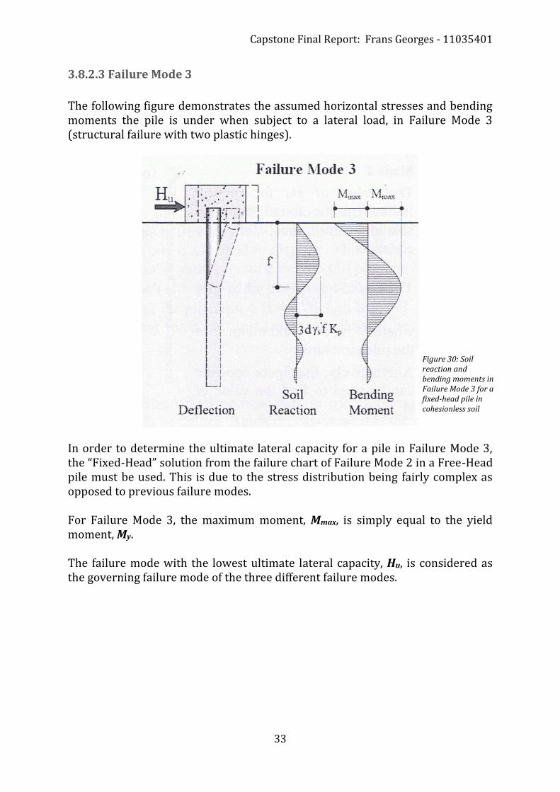
3.7.2.3 Failure Mode 3
The following figure demonstrates the assumed horizontal stresses and bending moments the pile is under when subject to a lateral load, in Failure Mode 3 (structural failure with two plastic hinges).
In order to determine the ultimate lateral capacity for a pile in Failure Mode 3, the “Fixed-Head” solution from the failure chart of Failure Mode 2 in a Free-Head pile must be used. This is due to the stress distribution being fairly complex as opposed to previous failure modes. For Failure Mode 3, the maximum moment, Mmax, is simply equal to the yield moment, My. The failure mode with the lowest ultimate lateral capacity, Hu, is considered as the governing failure mode of the three different failure modes.
3.8 Single Pile Lateral Capacity in Cohesionless Soils
The failure methods for piles in cohesionless soils are the same as for piles in cohesive soils. The major difference is the stress distribution in the soil for each failure mode. It is assumed that in a cohesionless soil case that a section of the soil in front of the pile displaces on failure. Failure is deemed to occur when the pressure exceeds three times that of Rankine’s passive earth pressure.
Figure 23: Soil reaction and bending moments in Failure Mode 3 for a fixed-head pile in cohesive soil
Capstone Final Report: Frans Georges - 11035401
29
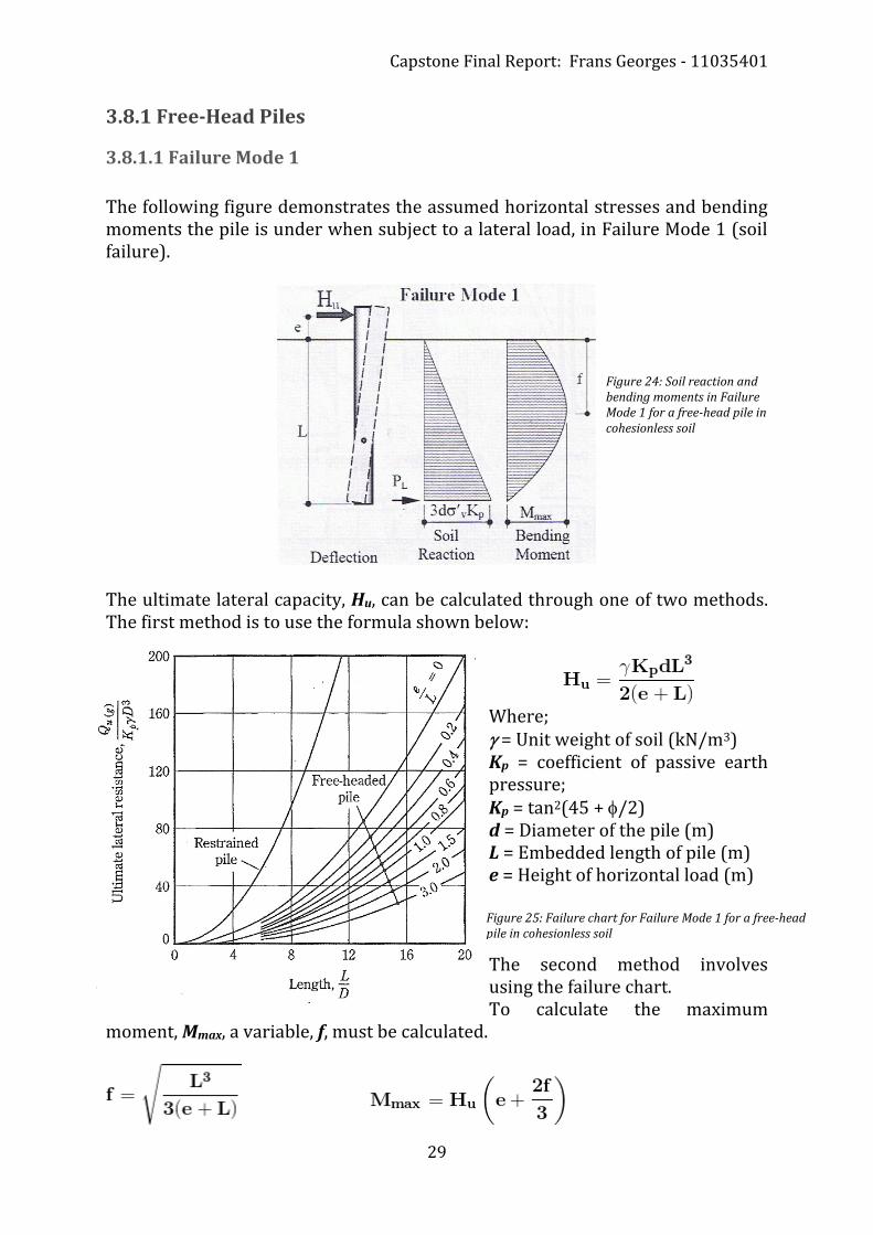
3.8.1 Free-Head Piles
3.8.1.1 Failure Mode 1
The following figure demonstrates the assumed horizontal stresses and bending moments the pile is under when subject to a lateral load, in Failure Mode 1 (soil failure).
The ultimate lateral capacity, Hu, can be calculated through one of two methods. The first method is to use the formula shown below:
Where; = Unit weight of soil (kN/m3) Kp = coefficient of passive earth pressure; Kp = tan2(45 + /2) d = Diameter of the pile (m) L = Embedded length of pile (m) e = Height of horizontal load (m) The second method involves using the failure chart. To calculate the maximum
moment, Mmax, a variable, f, must be calculated.
Figure 24: Soil reaction and bending moments in Failure Mode 1 for a free-head pile in cohesionless soil
Figure 25: Failure chart for Failure Mode 1 for a free-head pile in cohesionless soil

Capstone Final Report: Frans Georges - 11035401
30
3.8.1.2 Failure Mode 2
The following figure demonstrates the assumed horizontal stresses and bending moments the pile is under when subject to a lateral load, in Failure Mode 2 (structural failure).
The ultimate lateral capacity, Hu, can be calculated through one of two methods. The first method is to use the formula shown below:
Where; = Unit weight of soil (kN/m3) Kp = coefficient of passive earth pressure; Kp = tan2(45 + /2) d = Diameter of the pile (m) e = Height of horizontal load (m) My = Yield moment (kNm)
(kNm) The equation must be solved for Hu in order to determine the ultimate lateral capacity. The second method involves the use of the failure chart. For Failure Mode 2, the maximum moment, Mmax, is simply equal to the yield moment, My.
Figure 26: Soil reaction and bending moments in Failure Mode 2 for a free-head pile in cohesionless soil
Figure 27: Failure chart for Failure Mode 2 for a free-head pile in cohesionless soil

Capstone Final Report: Frans Georges - 11035401
31
3.8.2 Fixed-Head Piles
3.8.2.1 Failure Mode 1
The following figure demonstrates the assumed horizontal stresses and bending moments the pile is under when subject to a lateral load, in Failure Mode 1 (soil failure).
The ultimate lateral capacity, Hu, can be calculated through one of two methods. The first method is to use the formula shown below:
Where; = Unit weight of soil (kN/m3) d = Diameter of the pile (m) L = Embedded length of pile (m) Kp = coefficient of passive earth pressure; Kp = tan2(45 + /2) The second method to calculate Hu involves using the “Restrained Pile” solution in the failure chart of Mode 1 for the Free-Head pile in a cohesionless soil. The maximum moment, Mmax, for Failure Mode 1 in a fixed-head pile is calculated using the following relationship:
Figure 28: Soil reaction and bending moments in Failure Mode 1 for a fixed-head pile in cohesionless soil

Capstone Final Report: Frans Georges - 11035401
32
3.8.2.2 Failure Mode 2
The following figure demonstrates the assumed horizontal stresses and bending moments the pile is under when subject to a lateral load, in Failure Mode 2 (structural failure with one plastic hinge).
The ultimate lateral capacity, Hu, for a fixed-head pile in cohesionless soil in Failure Mode 2 can be calculated using the following relationship:
Where; = Unit weight of soil (kN/m3) d = Diameter of the pile (m) L = Embedded length of pile (m) Kp = coefficient of passive earth pressure; Kp = tan2(45 + /2) My = Yield moment (kNm) The maximum moment, Mmax, for Failure Mode 2 in a fixed-head pile can only be calculated after calculating f (depth at where maximum moment occurs). Both relationships are shown below:
Figure 29: Soil reaction and bending moments in Failure Mode 2 for a fixed-head pile in cohesionless soil
Capstone Final Report: Frans Georges - 11035401
33
3.8.2.3 Failure Mode 3
The following figure demonstrates the assumed horizontal stresses and bending moments the pile is under when subject to a lateral load, in Failure Mode 3 (structural failure with two plastic hinges).
In order to determine the ultimate lateral capacity for a pile in Failure Mode 3, the “Fixed-Head” solution from the failure chart of Failure Mode 2 in a Free-Head pile must be used. This is due to the stress distribution being fairly complex as opposed to previous failure modes. For Failure Mode 3, the maximum moment, Mmax, is simply equal to the yield moment, My. The failure mode with the lowest ultimate lateral capacity, Hu, is considered as the governing failure mode of the three different failure modes.
Figure 30: Soil reaction and bending moments in Failure Mode 3 for a fixed-head pile in cohesionless soil

Capstone Final Report: Frans Georges - 11035401
34
3.9 Horizontal Deflection of a Pile
The horizontal, or lateral deflection of a pile embedded into a soil layer can be determined using the elasticity theory in soil mechanics. This method, however, is not completely accurate as only an estimate is determined. This is due to the many assumptions being made in order to make the calculations much easier, such as complete homogeneity of the soil layers, the exclusion of viscoplastic soil behaviour, and also the exclusion of unsaturated and critical state analyses. Accurate results can only be obtained by controlled in-situ or laboratory testing, and by taking all these factors into account. For an undergraduate study, however, the following simplified methods are implemented, as explained in AS2159-1978.
3.9.1 Over-consolidated Clays
In a heavily over-consolidated clay layer, the soil modulus remains fairly uniform. This is taken into consideration to determine the ground-line displacement, , and rotation, , for a fixed-head and free-head pile. The varying equations are determined below: For a free-head pile:
For a fixed-head pile:
Where; H = Horizontal load (kN) Es = Elasticity modulus of soil (MPa) L = Embedded length of pile (m) M = Moment at ground level = Mapplied + (H × e) (kNm) IH = Load influence factor for displacement, free-head pile IM = Moment influence factor for displacement, free-head pile IH = Load influence factor for rotation, free-head pile IM = Moment influence factor for rotation, free-head pile IF = Load influence factor for displacement, fixed-head pile
Capstone Final Report: Frans Georges - 11035401
35
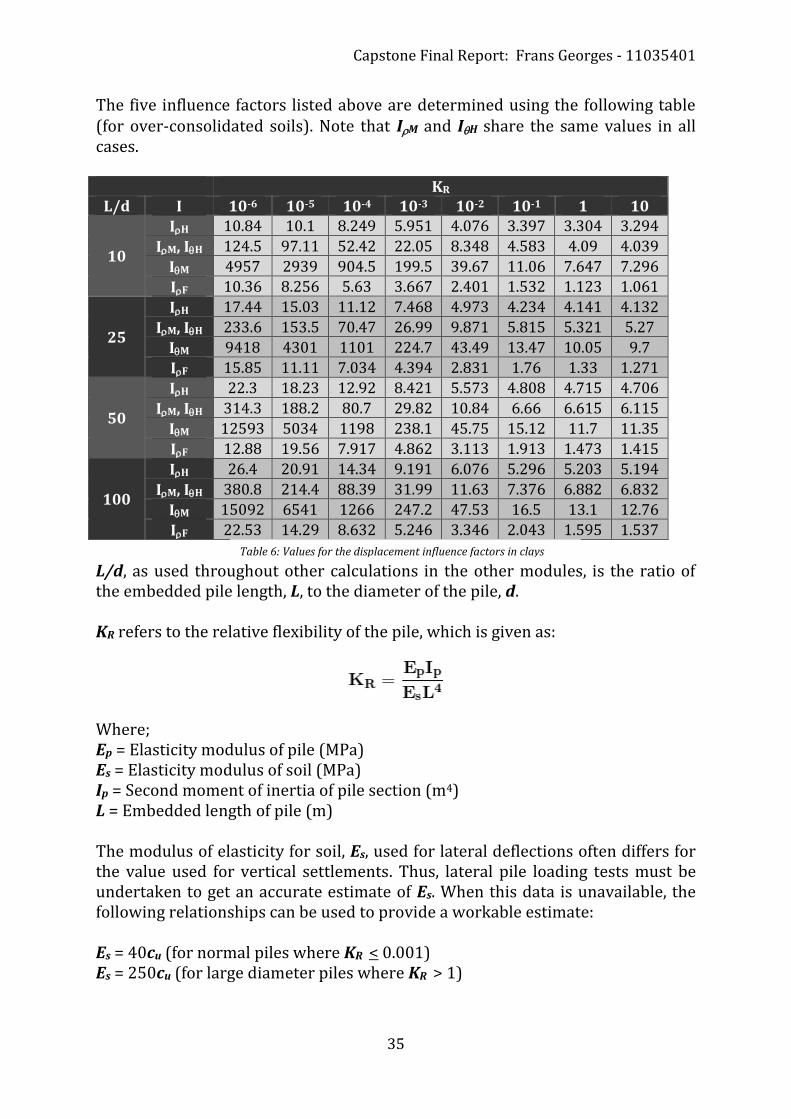
The five influence factors listed above are determined using the following table (for over-consolidated soils). Note that IM and IH share the same values in all cases.
KR L/d I 10-6 10-5 10-4 10-3 10-2 10-1 1 10
10
IH 10.84 10.1 8.249 5.951 4.076 3.397 3.304 3.294
IM, IH 124.5 97.11 52.42 22.05 8.348 4.583 4.09 4.039
IM 4957 2939 904.5 199.5 39.67 11.06 7.647 7.296
IF 10.36 8.256 5.63 3.667 2.401 1.532 1.123 1.061
25
IH 17.44 15.03 11.12 7.468 4.973 4.234 4.141 4.132
IM, IH 233.6 153.5 70.47 26.99 9.871 5.815 5.321 5.27
IM 9418 4301 1101 224.7 43.49 13.47 10.05 9.7
IF 15.85 11.11 7.034 4.394 2.831 1.76 1.33 1.271
50
IH 22.3 18.23 12.92 8.421 5.573 4.808 4.715 4.706
IM, IH 314.3 188.2 80.7 29.82 10.84 6.66 6.615 6.115
IM 12593 5034 1198 238.1 45.75 15.12 11.7 11.35
IF 12.88 19.56 7.917 4.862 3.113 1.913 1.473 1.415
100
IH 26.4 20.91 14.34 9.191 6.076 5.296 5.203 5.194
IM, IH 380.8 214.4 88.39 31.99 11.63 7.376 6.882 6.832
IM 15092 6541 1266 247.2 47.53 16.5 13.1 12.76
IF 22.53 14.29 8.632 5.246 3.346 2.043 1.595 1.537
L/d, as used throughout other calculations in the other modules, is the ratio of the embedded pile length, L, to the diameter of the pile, d. KR refers to the relative flexibility of the pile, which is given as:
Where; Ep = Elasticity modulus of pile (MPa) Es = Elasticity modulus of soil (MPa) Ip = Second moment of inertia of pile section (m4) L = Embedded length of pile (m) The modulus of elasticity for soil, Es, used for lateral deflections often differs for the value used for vertical settlements. Thus, lateral pile loading tests must be undertaken to get an accurate estimate of Es. When this data is unavailable, the following relationships can be used to provide a workable estimate: Es = 40cu (for normal piles where KR < 0.001) Es = 250cu (for large diameter piles where KR > 1)
Table 6: Values for the displacement influence factors in clays

Capstone Final Report: Frans Georges - 11035401
36
3.9.2 Normally-consolidated Clays and Sands
Unlike over-consolidated clays, the modulus of elasticity of normally-consolidated clays and sands increases linearly as depth increases. This is taken into consideration to determine the ground-line displacement, , and rotation, , for a fixed-head and free-head pile. The varying equations are determined below: For a free-head pile:
For a fixed-head pile:
Where; H = Horizontal load (kN) Nh = Rate of change of Young’s Modulus with depth (MPa/m)
Nh = Es / z L = Embedded length of pile (m) M = Moment at ground level = Mapplied + (H × e) (kNm) I’H = Load influence factor for displacement, free-head pile I’M = Moment influence factor for displacement, free-head pile I’H = Load influence factor for rotation, free-head pile I’M = Moment influence factor for rotation, free-head pile I’F = Load influence factor for displacement, fixed-head pile The table on the following page outlines the values for each influence factor, similarly to over-consolidated clays. In the table, the value for KN, the pile flexibility factor, is given by:
Where; Ep = Elasticity modulus of pile (MPa) Ip = Second moment of inertia of pile section (m4)

Capstone Final Report: Frans Georges - 11035401
37
KN
L/d I 10-6 10-5 10-4 10-3 10-2 10-1 >1
5
I’H 355 178 81 34.7 16.7 12.7 12.3
I’M, I’H 2940 1030 304 83 24.5 14.1 12.7
I’M 69000 14400 2460 401 68.8 22.8 17.6
I’F 1303 73.2 33.1 14.2 6.58 2.89 1.7
25
I’H 531 239 103 43.6 22.7 19.4 19
I’M, I’H 4830 1410 384 103 32.6 22.2 21.5
I’M 93500 16300 2710 437 81.8 35.3 30.2
I’F 208 98.1 41.3 18 8.4 3.58 2.5
100
I’H 653 282 120 50.4 28.3 25 24.7
I’M, I’H 5920 1640 437 115 40.5 30 29
I’M 104000 17600 2890 465 91.9 45.9 41.1
I’F 254 115 49.2 20.9 9.93 4.18 4.1
In the case of Nh not being available, the following table provides estimated values for Nh.
Soil Type Nh (MPa/m) Soft normally-consolidated clay 0.2
Normally-consolidated organic clay 0.1 Peat 0.04
Dry/moist loose sand 1.6 Dry/moist medium-dense sand 4.8
Dry/moist dense sand 12.6 For sand layers that are completely saturated, the Nh value is multiplied by 0.66.
Table 7: Values for the displacement influence factors in sand
Table 8: Typical values for Nh

Capstone Final Report: Frans Georges - 11035401
38
4 Computer Program
4.1 General Outline
The major focus of this project was to produce an efficient computer program in the sub-category of Deep Foundations and Piles in the geotechnical engineering field. The program was designed in Visual Basic 6, featuring a user-friendly, easy-to-navigate interface. The program covers eight modules in deep foundation design, each with their own required data inputs. These eight fields are:
- Undrained Axial Capacity (Cohesive Soils) - Drained Axial Capacity (Cohesionless Soils) - Hybrid Axial Capacity (Cohesive/Cohesionless Soils) - Free-Head Lateral Capacity (Cohesive Soils) - Fixed-Head Lateral Capacity (Cohesive Soils) - Free-Head Lateral Capacity (Cohesionless Soils) - Fixed-Head Lateral Capacity (Cohesionless Soils) - Vertical Settlement of a Single Pile
Each module will be discussed in detail in the coming subchapters. The program is solely designed for university students studying in the geotechnical field, and is not intended to be a substitute for hand-calculation, but rather utilised as a checking tool. Due to certain limitations of the program (which will be discussed in further detail for each module), some outputs may slightly vary when compared to hand calculations. Validation tests for the program have been carried out and will be discussed later in the report. While performing hand calculations, students may sometimes need to calculate a number of intermediate variables in order to work their way to a final answer. The modules within this program each have a number of appropriate intermediate variables that a student can compare their work with. This is done so that the student does not only have the final answer to compare their work to, thus making the checking of their hand calculations easier to verify in the case of a mistake during an intermediate step, leading to the incorrect valuation of a certain variable. As a whole, the program is suitable for very basic deep foundation calculations, thus the reason for it being designed for students, mainly at an introductory stage of geotechnical engineering.

Capstone Final Report: Frans Georges - 11035401
39
4.2 Undrained Axial Capacity (Cohesive Soils)
As this was the first module to be designed for the program, a certain layout and necessary amount of input is given to the user, which followed the same trend for the other seven modules within the program, particularly for the other two axial capacity modules. For this module to run successfully, the user is required to select the number of soil layers (from 1 to a maximum of 5), the diameter of the pile, in metres, the length of the embedded pile within each layer, in metres, and the undrained cohesion of each clay layer, in kilopascals. The outputs given by this module, based on the user input, are the adhesion reduction ()values for each layer, the pile surface area of each embedded length, in square metres, the total length of the pile, in metres, the Length/Diameter ratio, a Reduction Factor (Rs), the undrained cohesion at the base of the pile, in kilopascals, a bearing capacity factor (N’c) and the area of the base of the pile, in square metres. In order to calculate the value for each clay layer by hand calculations, the chart shown earlier in the report (Figure 9) is used, by lining up the undrained shear strength/cohesion of the soil with the line solution and reading off the y-axis to get the reduction factor. In order for the program to successfully calculate the adhesion factor (with little error), equations for the curve had to be determined. The resulting equations in this case were:
The plot below shows the above equations plotted together:
Figure 31: Plot of self-determined equations for the adhesion reduction factor
Capstone Final Report: Frans Georges - 11035401
40
As can be seen in the previous figure, a fairly accurate representation of the adhesion reduction factor graph is created by using these two equations. The equations were determined through the use of Microsoft Excel; by plotting certain points and graphing a trendline with a fifth order polynomial, fairly accurate results can be obtained. This, in turn, makes the coding much more sensitive whilst typing, but tends to yield better results than a simpler equation would yield in the end. The outputs for each layer, along with the general outputs, are then used in the ultimate axial capacity equation in order to determine the final undrained axial capacity of the pile. The figure is rounded to zero decimal places in order to produce a round number and is outputted for the user.
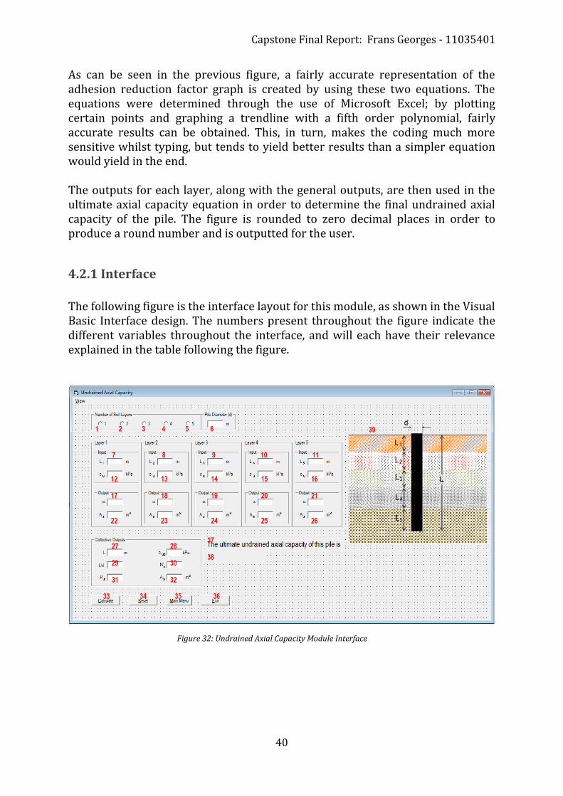
4.2.1 Interface
The following figure is the interface layout for this module, as shown in the Visual Basic Interface design. The numbers present throughout the figure indicate the different variables throughout the interface, and will each have their relevance explained in the table following the figure.
Figure 32: Undrained Axial Capacity Module Interface

Capstone Final Report: Frans Georges - 11035401
41
# Code Name Type Comment 1 Opt1 Option Button, Input One Soil Layer 2 Opt2 Option Button, Input Two Soil Layers 3 Opt3 Option Button, Input Three Soil Layers 4 Opt4 Option Button, Input Four Soil Layers 5 Opt5 Option Button, Input Five Soil Layers 6 d Text Box, Input Diameter of Pile (m) 7 L1 Text Box, Input Pile length in Layer 1 (m) 8 L2 Text Box, Input Pile length in Layer 2 (m) 9 L3 Text Box, Input Pile length in Layer 3 (m)
10 L4 Text Box, Input Pile length in Layer 4 (m) 11 L5 Text Box, Input Pile length in Layer 5 (m) 12 cu1 Text Box, Input Undrained cohesion of Layer 1 (kPa) 13 cu2 Text Box, Input Undrained cohesion of Layer 2 (kPa) 14 cu3 Text Box, Input Undrained cohesion of Layer 3 (kPa) 15 cu4 Text Box, Input Undrained cohesion of Layer 4 (kPa) 16 cu5 Text Box, Input Undrained cohesion of Layer 5 (kPa) 17 alpha1 Text Box, Output Adhesion reduction factor of Layer 1 18 alpha2 Text Box, Output Adhesion reduction factor of Layer 2 19 alpha3 Text Box, Output Adhesion reduction factor of Layer 3 20 alpha4 Text Box, Output Adhesion reduction factor of Layer 4 21 alpha5 Text Box, Output Adhesion reduction factor of Layer 5 22 As1 Text Box, Output Surface Area of Pile in Layer 1 (m2) 23 As2 Text Box, Output Surface Area of Pile in Layer 2 (m2) 24 As3 Text Box, Output Surface Area of Pile in Layer 3 (m2) 25 As4 Text Box, Output Surface Area of Pile in Layer 4 (m2) 26 As5 Text Box, Output Surface Area of Pile in Layer 5 (m2) 27 L Text Box, Output Total Length of Pile (m) 28 cub Text Box, Output Undrained cohesion at base (kPa) 29 Ldivd Text Box, Output Length/diameter ratio 30 Nc Text Box, Output Bearing capacity factor 31 Rs Text Box, Output Reduction factor 32 Ab Text Box, Output Area of pile base (m2) 33 Calc Command Button Calculates the Undrained Axial Capacity
34 Reset Command Button Resets the module, clears all input and output data
35 Menu Command Button Returns to Main Menu 36 Exit Command Button Closes the entire program
37 Label73 Label, Output Shows the text “The ultimate undrained axial capacity of this pile is” after calculating the result. Hidden at startup.
38 Result Label, Output Shows the final result (kN)
39 uac1, … , uac5 Picture Shows one of five different images depicting the amount of soil layers chosen for the problem.
Table 9: Undrained Axial Capacity Module Variables

Capstone Final Report: Frans Georges - 11035401
42
4.2.2 Assumptions and Limitations
Assumptions in this module include:
- All soil layers are completely homogenous, - All soil layers are completely undrained, - All soil layers in this certain problem are cohesive, i.e. clay, and no
cohesionless soils are present, - The pile diameter remains exactly the same throughout the length of the
pile, - The undrained cohesion value for each layer remains exactly the same
throughout the whole layer, - The layer interfaces are completely horizontal, with no inclination at any
angle, - The pile is embedded vertically, perfectly perpendicular to the soil, and - The user has predetermined values for the undrained cohesion of each
layer and pile dimensions. Limitations of this module are:
- A maximum of five soil layers can be selected, - No option to apply any external forces or pressures, - Only clays with undrained capacities of up to 200kPa may be entered, - No factors of safety applied. This may lead to inaccurate estimates in some
cases, - The pile is a solid cylindrical shape; other shaped cross sections (such as a
square cross-section) and hollow cross-sections are not available, and - The limited accuracy of the depiction of the adhesion reduction factor with
the fifth order polynomial equation determined earlier; it determines fairly accurate results but never exact as one would read off the actual graph discussed in the Theory section. The accuracy of the adhesion reduction factor tends to decrease as the value of the undrained cohesion rises, thus why the input undrained cohesion is limited to 200 kPa per soil layer

Capstone Final Report: Frans Georges - 11035401
43
4.3 Drained Axial Capacity (Cohesionless Soils)
Following from the general design of the Undrained Axial Capacity module, this module is very similar except it is dealing solely with cohesionless soils, i.e. sandy soils and gravel. The main difference between this module and the undrained module is that this module introduces the use of the water table, which is necessary in the calculation of drained axial capacity, and other input variables that are discussed below.
For the module to run successfully, the user is required to take the following steps: - Select the number of soil layers (minimum of one, maximum of five), - Enter the pile diameter, d, in metres, - Enter the depth of the water table, in metres, - Select a soil consistency (either Loose, Medium or Dense soil), - Select a method of installation for the pile (either Driven or Bored/Cast In-
situ), - Enter the embedment pile length for each soil layer, Li, in metres, - Enter the unit weight of each soil layer, in kilo newtons per cubic metre,
and - Click the “Calculate” button to generate the result, Pu, in kilo newtons.
The outputs in this module are much less complicated than in the first module, as there is no adhesion reduction factor with a complicated equation to deal with. For each soil layer, the surface area of the length of pile in the soil layer, As, is calculated, in square metres. Two other variables, top and bottom, are calculated, in kilopascals. These values represent the stresses at the very top and bottom of each layer. These values interact with the values of the following layer; the stress at the bottom of one layer is used as the stress at the top of the following layer. The initial layer always begins with a stress of zero at the top, and with a value of the entered unit weight, , multiplied by the embedded length, Li, to generate a value for the stress at the bottom of the layer. The following layer then uses this same value as its initial stress at the top, while the stress at the bottom is calculated using a trapezoidal technique (this is clearly shown in the code, check Appendix for full transcript). The general outputs include the total length of the pile, L, in metres, a shaft friction coefficient, F, a bearing capacity factor, Nq, the vertical effective stress at the base of the pile, ’vb, in kilopascals, and the area of the base of the pile, Ab, in square metres. The use of the water table, however, makes this slightly more complicated to code in comparison to the first module. The technique used to seamlessly incorporate the water table without interrupting the flow of the module, is through splitting the layer where the water table resides.

Capstone Final Report: Frans Georges - 11035401
44
For example, taking the following problem:
Where: d = 0.5m L1 = 3m L2 = 4m 1 = 15 kN/m3 2 = 20 kN/m3 WT = 2m
The user would select two soil layers, and enter the given values into the module in the appropriate inputs, along with a choice for the soil consistency and pile installation method. After selecting two layers, only two input layers are visible for input. However, as the water table resides in the first layer, the third input layer becomes visible after the user has clicked “Calculate”. The third input layer will then have the data for the initial second layer, in a saturated state (as it is under the location of the water table). Therefore, in this example, L3 would have a value of 4m, and 3 would have a value of (20 – 9.8) kN/m3 = 10.2 kN/m3. The second input layer will then represent the saturated portion of the first initial layer (below the water table). Therefore, in this example, L2 would have a new value of (3 – 2) m = 1m, and 2 would have a value of (15 – 9.8) kN/m3 = 5.2 kN/m3. Finally, the first input layer will represent the dry portion of the first initial layer (above the water table). Therefore, in this example, L1 would have a new value of 2m, and 1 would keep its initial value of 15 kN/m3. This technique is only coded into the program in cases where the water table resides within a layer; problems that have the water table sitting at a layer interface or at the top do not need to implement this method as none of the layers require splitting. Any saturated layers, however, will have their corresponding unit weight reduced by a value of 9.8 kN/m3, to take the effect of water into consideration.
Figure 33: Example Drained Axial Capacity problem

Capstone Final Report: Frans Georges - 11035401
45
4.3.1 Interface
The following figure is the interface layout for this module, as shown in the Visual Basic Interface design. The numbers present throughout the figure indicate the different variables throughout the interface, and will each have their relevance explained in the table following the figure.
# Code Name Type Comment 1 Opt1 Option Button, Input One Soil Layer 2 Opt2 Option Button, Input Two Soil Layers 3 Opt3 Option Button, Input Three Soil Layers 4 Opt4 Option Button, Input Four Soil Layers 5 Opt5 Option Button, Input Five Soil Layers 6 d Text Box, Input Diameter of Pile (m) 7 wtd Text Box, Input Water table depth (m) 8 optL Option Button, Input Loose soil 9 optM Option Button, Input Medium density soil
10 optD Option Button, Input Dense soil 11 optDRV Option Button, Input Driven pile 12 optBCI Option Button, Input Bored/Cast in-situ pile 13 L1 Text Box, Input Pile length in Layer 1 (m) 14 L2 Text Box, Input Pile length in Layer 2 (m) 15 L3 Text Box, Input Pile length in Layer 3 (m) 16 L4 Text Box, Input Pile length in Layer 4 (m) 17 L5 Text Box, Input Pile length in Layer 5 (m) 18 gamma1 Text Box, Input Unit weight of Layer 1 (kN/m3)
Figure 34: Drained Axial Capacity Module Interface

Capstone Final Report: Frans Georges - 11035401
46
19 gamma2 Text Box, Input Unit weight of Layer 2 (kN/m3) 20 gamma3 Text Box, Input Unit weight of Layer 3 (kN/m3) 21 gamma4 Text Box, Input Unit weight of Layer 4 (kN/m3) 22 gamma5 Text Box, Input Unit weight of Layer 5 (kN/m3) 23 As1 Text Box, Output Surface Area of Pile in Layer 1 (m2) 24 As2 Text Box, Output Surface Area of Pile in Layer 2 (m2) 25 As3 Text Box, Output Surface Area of Pile in Layer 3 (m2) 26 As4 Text Box, Output Surface Area of Pile in Layer 4 (m2) 27 As5 Text Box, Output Surface Area of Pile in Layer 5 (m2) 28 sigmatop1 Text Box, Output Vert. Eff. Stress at top of Layer 1 (kPa) 29 sigmatop2 Text Box, Output Vert. Eff. Stress at top of Layer 2 (kPa) 30 sigmatop3 Text Box, Output Vert. Eff. Stress at top of Layer 3 (kPa) 31 sigmatop4 Text Box, Output Vert. Eff. Stress at top of Layer 4 (kPa) 32 sigmatop5 Text Box, Output Vert. Eff. Stress at top of Layer 5 (kPa) 33 sigmabot1 Text Box, Output Vert. Eff. Stress bottom of Layer 1 (kPa) 34 sigmabot2 Text Box, Output Vert. Eff. Stress bottom of Layer 2 (kPa) 35 sigmabot3 Text Box, Output Vert. Eff. Stress bottom of Layer 3 (kPa) 36 sigmabot4 Text Box, Output Vert. Eff. Stress bottom of Layer 4 (kPa) 37 sigmabot5 Text Box, Output Vert. Eff. Stress bottom of Layer 5 (kPa) 38 L Text Box, Output Total Length of Pile (m) 39 sigmavb Text Box, Output Vertical Effective Stress at base (kPa) 40 F Text Box, Output Shaft friction coefficient 41 Ab Text Box, Output Area of pile base (m2) 42 Nq Text Box, Output Bearing capacity factor 43 Calc Command Button Calculates the Drained Axial Capacity
44 Reset Command Button Resets the module, clears all input and output data
45 Menu Command Button Returns to Main Menu 46 Exit Command Button Closes the entire program
47 Label41 Label, Output Shows the text “The ultimate drained axial capacity of this pile is” after calculating the result. Hidden at startup.
48 DACResult Label, Output Shows the final result (kN)
49 dac1, … , dac5 Picture Shows one of five different images depicting the amount of soil layers chosen for the problem.
Table 10: Drained Axial Capacity Module Variables

Capstone Final Report: Frans Georges - 11035401
47
4.3.2 Assumptions and Limitations
Assumptions for this module include:
- All soils are completely homogenous, - All soils above the water table are completely dry, - All soils below the water table are completely saturated, - All soils are cohesionless, i.e. sand or gravel, and no cohesive soils are
present, - Unsaturated states are ignored, - The pile diameter remains exactly the same throughout the length of the
pile, - The unit weight for each layer remains exactly the same throughout the
whole layer, - The layer interfaces are completely horizontal, with no inclination at any
angle, - If a value of zero is entered for the water table, it is assumed that the water
table is located right at the top of the first layer, thus making every layer saturated,
- If a value equal to or greater than the length of the pile is entered for the water table, it is assumed that the water table has no effect on the axial capacity, thus making every layer dry,
- The pile is embedded vertically, perfectly perpendicular to the soil, and - The user has predetermined values for the undrained cohesion of each
layer and pile dimensions. Limitations of this module are:
- Calculations involving selections of one, two or three layers will only display results; although an option for four and five layers are provided and coded into the module, the issue as to why the results would not be displayed (module does not crash) could not be determined, despite following the exact coding method used to code the calculations for one, two and three layers. This can be seen in the code transcripts in the Appendix,
- No option to apply any external forces or pressures, - No factors of safety applied. This may lead to inaccurate estimates in some
cases, and - The pile is a solid cylindrical shape; other shaped cross sections (such as a
square cross-section) and hollow cross-sections are not available

Capstone Final Report: Frans Georges - 11035401
48
4.4 Hybrid Axial Capacity (Cohesive and Cohesionless Soils)
For this module, it is basically a cross between the first two modules, and thus a much more realistic representation of a simple real-life geotechnical problem. The coding is slightly more complex in comparison to the last two modules, due to the many checks being run at the same time and the splitting/switching over of layers and layer properties to correctly calculate the axial capacity. To run this module correctly, the user is required to:
- Select a number of soil layers (either two or three), - Enter a value for the diameter of the pile, d, in metres, - Enter a value for the water table depth, in metres, - Select the type of soil for each layer (either Cohesive or Cohesionless)
(NOTE: If a cohesionless soil is selected, the user is required to select the soil consistency – either Loose, Medium or Dense – and the method of installation – either Driven or Bored/Cast In-Situ. If the user selects a cohesive soil type, the Soil Consistency and Pile Installation choices are immediately disabled),
- Enter the length of pile in each soil layer, Li, in metres, - Enter the unit weight of each soil layer, , in kilo newtons per cubic metre, - Enter the undrained cohesion, cu, for any cohesive soil layers (NOTE: if a
soil layer is selected as ‘cohesionless’, the cohesion value, cu, and the adhesion reduction factor, , are immediately noted with “N/A”), and
- Click the “Calculate” button to generate the result, Pu, in kilo newtons. Considering that this is a cross between the first two modules, the outputs consist of all the varying outputs in the first two modules, all in one module. This means that for cohesive soils, the fifth order polynomial equation used to calculate the adhesion reduction factor, , is used. The trapezoidal technique of calculating stresses for the top and bottom (top and bottom) of each layer from the second module is utilised in this module, however, it is used for all types of soils rather than just for cohesionless soils. The shaft resistance, Ps, for each soil layer is now shown in order to make calculating the axial capacity easier. This is due to the fact that the calculation of the shaft resistance uses different methods for cohesive and cohesionless soils. The list of general outputs involves a mix of all the outputs present in the first two modules (which were discussed earlier in their respective sections), along with the base resistance, Pb, measured in kilo newtons. Using the Ps and Pb values, the program can then determine the axial capacity, Pu, in kilo newtons. This module also uses the method of splitting layers where the water table resides in order to effectively solve a problem, as was discussed in the section of the report explaining the Drained Axial Capacity module of the program. In this module, however, this method requires slightly more coding effort due to the inevitable instance of moving one layer properties to the next, where the type of

Capstone Final Report: Frans Georges - 11035401
49
soil is not the same. For example, in a problem containing two soil layers – one cohesive and one cohesionless – with the water table sitting in the middle of the top cohesive layer, when the ‘splitting method’ is carried out, the properties for Layer 2 get moved over to Layer 3, which is of no fuss as there was no data in Layer 3. However, after splitting the initial Layer 1 to be spread over Layer 1 and Layer 2 (due to the water table), the cohesive properties of Layer 1 are being transferred to Layer 2, which was accommodating a cohesionless soil. The process of switching layer selections and re-enabling and disabling certain properties necessarily required a fair amount of trial-and-error coding methods.
4.4.1 Interface
The following figure is the interface layout for this module, as shown in the Visual Basic Interface design. The numbers present throughout the figure indicate the different variables throughout the interface, and will each have their relevance explained in the table following the figure.
Figure 35: Hybrid Axial Capacity Module Interface

Capstone Final Report: Frans Georges - 11035401
50
# Code Name Type Comment 1 Opt2L Option Button, Input Two Soil Layers 2 Opt3L Option Button, Input Three Soil Layers 3 d Text Box, Input Diameter of Pile (m) 4 wtd Text Box, Input Water table depth (m) 5 co1 Option Button, Input Cohesive Soil for Layer 1 6 co2 Option Button, Input Cohesive Soil for Layer 2 7 co3 Option Button, Input Cohesive Soil for Layer 3 8 col1 Option Button, Input Cohesionless Soil for Layer 1 9 col2 Option Button, Input Cohesionless Soil for Layer 2
10 col3 Option Button, Input Cohesionless Soil for Layer 3 11 SCL1 Option Button, Input Loose Soil for Layer 1 12 SCL2 Option Button, Input Loose Soil for Layer 2 13 SCL3 Option Button, Input Loose Soil for Layer 3 14 SCM1 Option Button, Input Medium Soil for Layer 1 15 SCM2 Option Button, Input Medium Soil for Layer 2 16 SCM3 Option Button, Input Medium Soil for Layer 3 17 SCD1 Option Button, Input Dense Soil for Layer 1 18 SCD2 Option Button, Input Dense Soil for Layer 2 19 SCD3 Option Button, Input Dense Soil for Layer 3 20 PID1 Option Button, Input Driven Pile in Layer 1 21 PID2 Option Button, Input Driven Pile in Layer 2 22 PID3 Option Button, Input Driven Pile in Layer 3 23 PIB1 Option Button, Input Bored/Cast In-situ Pile in Layer 1 24 PIB2 Option Button, Input Bored/Cast In-situ Pile in Layer 2 25 PIB3 Option Button, Input Bored/Cast In-situ Pile in Layer 3 26 L1 Text Box, Input Pile length in Layer 1 (m) 27 L2 Text Box, Input Pile length in Layer 2 (m) 28 L3 Text Box, Input Pile length in Layer 3 (m) 29 L4 Text Box, Input Pile length in Layer 4 (m) 30 gamma1 Text Box, Input Unit weight of Layer 1 (kN/m3) 31 gamma2 Text Box, Input Unit weight of Layer 2 (kN/m3) 32 gamma3 Text Box, Input Unit weight of Layer 3 (kN/m3) 33 gamma4 Text Box, Input Unit weight of Layer 4 (kN/m3) 34 cu1 Text Box, Input Undrained cohesion of Layer 1 (kPa) 35 cu2 Text Box, Input Undrained cohesion of Layer 2 (kPa) 36 cu3 Text Box, Input Undrained cohesion of Layer 3 (kPa) 37 cu4 Text Box, Input Undrained cohesion of Layer 4 (kPa) 38 As1 Text Box, Output Surface Area of Pile in Layer 1 (m2) 39 As2 Text Box, Output Surface Area of Pile in Layer 2 (m2) 40 As3 Text Box, Output Surface Area of Pile in Layer 3 (m2) 41 As4 Text Box, Output Surface Area of Pile in Layer 4 (m2) 42 sigtop1 Text Box, Output Vert. Eff. Stress at top of Layer 1 (kPa) 43 sigtop2 Text Box, Output Vert. Eff. Stress at top of Layer 2 (kPa) 44 sigtop3 Text Box, Output Vert. Eff. Stress at top of Layer 3 (kPa) 45 sigtop4 Text Box, Output Vert. Eff. Stress at top of Layer 4 (kPa) 46 sigbot1 Text Box, Output Vert. Eff. Stress bottom of Layer 1 (kPa)

Capstone Final Report: Frans Georges - 11035401
51
47 sigbot2 Text Box, Output Vert. Eff. Stress bottom of Layer 2 (kPa) 48 sigbot3 Text Box, Output Vert. Eff. Stress bottom of Layer 3 (kPa) 49 sigbot4 Text Box, Output Vert. Eff. Stress bottom of Layer 4 (kPa) 50 alpha1 Text Box, Output Adhesion reduction factor of Layer 1 51 alpha2 Text Box, Output Adhesion reduction factor of Layer 2 52 alpha3 Text Box, Output Adhesion reduction factor of Layer 3 53 alpha4 Text Box, Output Adhesion reduction factor of Layer 4 54 Ps1 Text Box, Output Shaft Resistance of Layer 1 (kN) 55 Ps2 Text Box, Output Shaft Resistance of Layer 2 (kN) 56 Ps3 Text Box, Output Shaft Resistance of Layer 3 (kN) 57 Ps4 Text Box, Output Shaft Resistance of Layer 4 (kN) 58 L Text Box, Output Total Length of Pile (m) 59 Ab Text Box, Output Area of pile base (m2) 60 Ldivd Text Box, Output Length/Diameter Ratio 61 F Text Box, Output Shaft friction coefficient 62 Rs Text Box, Output Reduction factor 63 Nq Text Box, Output Bearing capacity factor (cohesionless) 64 cub Text Box, Output Undrained cohesion at base (kPa) 65 sigmavb Text Box, Output Vertical Effective Stress at Base (kPa) 66 Nc Text Box, Output Bearing capacity factor (cohesive) 67 Pb Text Box, Output Base Resistance of Pile (kN) 68 Calc Command Button Calculates the Hybrid Axial Capacity
69 Reset Command Button Resets the module, clears all input and output data
70 Menu Command Button Returns to Main Menu 71 Exit Command Button Closes the entire program
72 Label107 Label, Output Shows the text “The ultimate axial capacity of this pile is” after calculating the result. Hidden at startup.
73 HACRes Label, Output Shows the final result (kN)
74 hac1, hac2 Picture Shows one of two different images depicting the amount of soil layers chosen for the problem.
Table 11: Hybrid Axial Capacity Module Variables

Capstone Final Report: Frans Georges - 11035401
52
4.4.2 Assumptions and Limitations
Assumptions for this module include:
- All soils are completely homogenous, - All soils above the water table are completely dry, - All soils below the water table are completely saturated, - Unsaturated states are ignored, - The pile diameter remains exactly the same throughout the length of the
pile, - The unit weight for each layer remains exactly the same throughout the
whole layer, - The undrained cohesion value for each layer remains exactly the same
throughout the whole layer, - The layer interfaces are completely horizontal, with no inclination at any
angle, - If a value of zero is entered for the water table, it is assumed that the water
table is located right at the top of the first layer, thus making every layer saturated,
- If a value equal to or greater than the length of the pile is entered for the water table, it is assumed that the water table has no effect on the axial capacity, thus making every layer dry,
- The pile is embedded vertically, perfectly perpendicular to the soil, and - The user has predetermined values for the undrained cohesion of each
layer and pile dimensions. Limitations of this module are:
- A maximum of three soil layers can be selected, - The pile is a solid cylindrical shape; other shaped cross sections (such as a
square cross-section) and hollow cross-sections are not available - Only clays with undrained capacities of up to 200kPa may be entered, - No option to apply any external forces or pressures, - No factors of safety applied. This may lead to inaccurate estimates in some
cases, and - The limited accuracy of the depiction of the adhesion reduction factor with
the fifth order polynomial equation determined earlier; it determines fairly accurate results but never exact as one would read off the actual graph discussed in the Theory section. The accuracy of the adhesion reduction factor tends to decrease as the value of the undrained cohesion rises, thus why the input undrained cohesion is limited to 200 kPa per soil layer.

Capstone Final Report: Frans Georges - 11035401
53
4.5 Free-Head Lateral Capacity (Cohesive Soils)
The lateral capacity modules are significantly shorter to code in comparison to the axial capacity modules, but required equally as much work due to the vast amount of equation derivation that is required to produce accurate models. This specific module was the first to be coded out of the four lateral capacity modules and was aimed to act as a benchmark to the three modules that would follow it. The basic interface layout is similar to that used in the axial capacity interfaces, keeping it as user-friendly as possible. In order to run this module properly, the user is required to:
- Enter the diameter of the pile, d, in metres, - Enter the embedded length, L, of the pile, in metres, - Enter the height above the ground at which the horizontal load will act, e,
in metres, - Enter the undrained cohesion for the cohesive soil, cu, in kilopascals, - Enter the yield moment, My, in kilo Newton metres, and - Click “Calculate” to determine the Failure Mode, Maximum Lateral
Capacity and Maximum Moment Capacity. From first glance, this module seems to have very few outputs in comparison to the axial capacity modules. Most of the outputs are computed with fairly simple equations that have been outlined earlier in the report. This is the case for the Length/diameter ratio and the e/diameter ratio. The problematic section is determining the ultimate lateral capacity, Hu, for Failure Mode 1. As is explained in the theory earlier in the report, the method in which to determine this value is to first determine S, a factor which is calculated by using Figure 18, where the Length/diameter ratio (x-axis) is lined up with the solution on the graph representing the corresponding e/diameter ratio. The corresponding value on the y-axis is then read as the value for S. Due to the (almost) linear nature of the solutions for e/d values from 0 to 16 on the graph, certain linear solutions were determined in Excel for use within this module. The following table summarises all of the equations for each value of e/d that is present on the graph. Note that the results produced from these equations are not exact due to the lines mostly being a trendline, or line of best fit for the given range.

Capstone Final Report: Frans Georges - 11035401
54
e/d Equation Range
0
1
2
4
8
16
In the case of getting an e/d value which is not listed in the table above, a linear interpolation process is carried out with the above equations in order to determine the value for S. This value is then used to determine the ultimate lateral capacity, Hu, of the pile in Failure Mode 1. This value is imperative for the calculations of both f and g variables, and for the calculation of the maximum moment in Failure Mode 1.
Table 12: Self-determined equations for the Free-Head Lateral Capacity (Cohesive) Module

Capstone Final Report: Frans Georges - 11035401
55
For Failure Mode 2, the factor L is much easier to calculate, as a formula exists, guaranteeing an accurate answer. Using this calculated value, the ultimate lateral capacity for Failure Mode 2 is calculated. The maximum moment for Failure Mode 2 is simply taken as the Yield Moment that was entered by the user. The governing Failure Mode is then determined as the mode with the lesser of the lateral capacities. This lateral capacity is the ultimate lateral capacity and the corresponding maximum moment is the maximum moment capacity of the pile, both which the module will display, with an image of the governing Failure Mode.
4.5.1 Interface
The following figure is the interface layout for this module, as shown in the Visual Basic Interface design. The numbers present throughout the figure indicate the different variables throughout the interface, and will each have their relevance explained in the table following the figure.
Figure 36: Free-Head Lateral Capacity (Cohesive Soils) Module Interface

Capstone Final Report: Frans Georges - 11035401
56
# Code Name Type Comment 1 d Text Box, Input Diameter of pile (m) 2 L Text Box, Input Embedded length of pile (m) 3 e Text Box, Input Height of load above the ground (m) 4 cu Text Box, Input Soil Cohesion (kPa) 5 My Text Box, Input Yield Moment (kNm) 6 Ldivd Text Box, Output Length/diameter ratio 7 edivd Text Box, Output e/diameter ratio 8 f Text Box, Output Depth of Maximum moment (m)
9 g Text Box, Output Depth from the maximum moment to the pile base (m)
10 Hu1 Text Box, Output Ultimate lateral capacity for Failure Mode 1 (kN)
11 Mmax1 Text Box, Output Maximum moment for Failure Mode 1 (kNm)
12 lam1 Text Box, Output Lateral capacity factor for Failure Mode 1
13 Hu2 Text Box, Output Ultimate lateral capacity for Failure Mode 2 (kN)
14 Mmax2 Text Box, Output Maximum moment for Failure Mode 2 (kNm)
15 lam2 Text Box, Output Lateral capacity factor for Failure Mode 2 16 Calc Command Button Calculates the Free-Head Lateral Capacity
17 Reset Command Button Resets the module, clears all input and output data
18 Menu Command Button Returns to Main Menu 19 Exit Command Button Closes the entire program
20 Label33 Label, Output Shows the text “The failure mode for this pile is” after calculation. Hidden at startup.
21 ResFM Label, Output Displays the governing failure mode
22 Label34 Label, Output Shows the text “The maximum lateral capacity for this pile is” after calculation. Hidden at startup.
23 ResHu Label, Output Displays the maximum lateral capacity (kN)
24 Label35 Label, Output Shows the text “The maximum moment capacity for this pile is” after calculation. Hidden at startup.
25 ResMmax Label, Output Displays the maximum moment capacity (kNm)
26 fm1, fm2 Picture Shows one of two different images depicting the governing failure mode for the pile
Table 13: Free-Head Lateral Capacity (Cohesive) Module Variables

Capstone Final Report: Frans Georges - 11035401
57
4.5.2 Assumptions and Limitations
Assumptions for this module include:
- The soil is completely homogenous, - The entire depth at which the pile is embedded is of the same soil, - The cohesion of the soil remains the same throughout, - The soil is completely undrained, - The soil is completely cohesive, no cohesionless soils present, - The pile diameter remains exactly the same throughout the length of the
pile, - The pile is embedded vertically, perfectly perpendicular to the soil, and - The user has predetermined values for the undrained cohesion of each
layer and pile dimensions.
Limitations for this module are:
- No choice for multiple layers. This allows for only very simple cases to be solved,
- The pile is a solid cylindrical shape; other shaped cross sections (such as a square cross-section) and hollow cross-sections are not available,
- The determined equations for the calculation of the lateral capacity factor for Failure Mode 1 tend to sometimes yield results that are not too accurate, thus affecting the final value for the ultimate lateral capacity in Failure Mode 1, and
- No option to apply any external forces or pressures.

Capstone Final Report: Frans Georges - 11035401
58
4.6 Fixed-Head Lateral Capacity (Cohesive Soils)
This module is very similar to the previous module, however is fairly simpler in terms of coding and determining the maximum lateral capacity. The main difference is that for a fixed-head pile, there are three failure modes to consider as opposed to the two in the previous module. The methods to determine the maximum lateral capacities and moments for the first two failure modes are very simple and accurate, as there are set equations to do so. In order to run this module correctly, the user is required to:
- Enter the diameter of the pile, d, in metres, - Enter the embedded length of the pile, L, in metres, - Enter the undrained cohesion for the cohesive soil, cu, in kilopascals, - Enter the yield moment, My, in kilo Newton metres, and - Click “Calculate” to determine the Failure Mode, Maximum Lateral
Capacity and Maximum Moment Capacity. As mentioned earlier, the lateral and moment capacity for the first two failure modes are determined by equations that have been explained earlier in the theory section of this report. The moment capacity in the third failure mode is taken simply as the yield moment entered by the user, but the lateral capacity is only determinable through using the “Fixed-Head” or “Restrained” solution in a graph used for Failure Mode 2 for free-head piles. Notice that when the previous module was dealing with Failure Mode 2 (for a free-head pile), an equation was used in place for this graph, as one was provided. For a restrained or fixed-head solution, however, no equation is provided and would therefore need to be determined. All of the following equations were determined by carefully plotting the restrained solution in Excel and setting up various logarithmic trendlines, as one trendline would be too inaccurate to represent the restrained solution.
The calculated y value is then multiplied by cud2 to determine the ultimate lateral capacity, Hu. As the restrained solution is only one possible solution, no interpolation is required, thus making the calculation of the lateral capacity very simple. The

Capstone Final Report: Frans Georges - 11035401
59
governing failure mode is chosen as the one with the least lateral capacity, and its accompanying moment as the maximum moment capacity.
4.6.1 Interface
The following figure is the interface layout for this module, as shown in the Visual Basic Interface design. The numbers present throughout the figure indicate the different variables throughout the interface, and will each have their relevance explained in the table following the figure.
Figure 37: Fixed-Head Lateral Capacity (Cohesive Soils) Module Interface

Capstone Final Report: Frans Georges - 11035401
60
# Code Name Type Comment 1 d Text Box, Input Diameter of pile (m) 2 L Text Box, Input Embedded length of pile (m) 3 cu Text Box, Input Soil Cohesion (kPa) 4 My Text Box, Input Yield Moment (kNm) 5 f Text Box, Output Depth of Maximum moment (m)
6 g Text Box, Output Depth from the maximum moment to the pile base (m)
7 Hu1 Text Box, Output Ultimate lateral capacity for Failure Mode 1 (kN)
8 Hu2 Text Box, Output Ultimate lateral capacity for Failure Mode 2 (kN)
9 Hu3 Text Box, Output Ultimate lateral capacity for Failure Mode 3 (kN)
10 Mmax1 Text Box, Output Maximum moment for Failure Mode 1 (kNm)
11 Mmax2 Text Box, Output Maximum moment for Failure Mode 2 (kNm)
12 Mmax2 Text Box, Output Maximum moment for Failure Mode 3 (kNm)
13 Calc Command Button Calculates the Fixed-Head Lateral Capacity
14 Reset Command Button Resets the module, clears all input and output data
15 Menu Command Button Returns to Main Menu 16 Exit Command Button Closes the entire program
17 Label33 Label, Output Shows the text “The failure mode for this pile is” after calculation. Hidden at startup.
18 Label34 Label, Output Shows the text “The maximum lateral capacity for this pile is” after calculation. Hidden at startup.
19 Label35 Label, Output Shows the text “The maximum moment capacity for this pile is” after calculation. Hidden at startup.
20 ResFM Label, Output Displays the governing failure mode
21 ResHu Label, Output Displays the maximum lateral capacity (kN)
22 ResMmax Label, Output Displays the maximum moment capacity (kNm)
23 fm1, fm2, fm3 Picture Shows one of three different images depicting the governing failure mode for the pile
4.6.2 Assumptions and Limitations
The assumptions and limitations for this module are identical to the previous module, with a similar limitation in terms of the use of self-determined equations for help in calculating lateral capacity.
Table 14: Fixed-Head Lateral Capacity (Cohesive) Module Variables

Capstone Final Report: Frans Georges - 11035401
61
4.7 Free-Head Lateral Capacity (Cohesionless Soils)
Similarly to the Free-Head Lateral Capacity of Cohesive Soils module, this module has two possible failure modes, and the properties for the first failure mode are much more straight forward to calculate. The second requires a vast range of self-determined equations, which will be discussed later. For this module to run, the user is required to:
- Enter the diameter of the pile, d, in metres, - Enter the embedded length, L, of the pile, in metres, - Enter the height above the ground at which the horizontal load will act, e,
in metres, - Enter the unit weight of the soil, , in kilo Newtons per cubic metre, - Enter the yield moment, My, in kilo Newton metres, - Enter the soil friction angle, , and - Click “Calculate” to determine the Failure Mode, Maximum Lateral
Capacity and Maximum Moment Capacity. The general outputs in this module are fairly simple to calculate, providing the user with the total effective vertical stress, ’v, the e/diameter ratio and the passive earth pressure coefficient, Kp, which all have their respective equations explained thoroughly in the Theory section of the report. This goes the same for the maximum lateral and moment capacities determined for the first failure mode. The maximum moment capacity for the second failure mode is taken simply as the yield moment which was entered by the user prior to calculations. To calculate the ultimate lateral capacity for the second failure mode, however, Figure 27 must be used when calculating the value manually. Therefore, to get an accurate representation of the figure in the module, a range of equations needed to be defined and programmed into the module. As the graph is presented in a logarithmic scale, a number of logarithmic trendlines were created for the plotted points in Microsoft Excel, for each solution of the e/d ratio. In doing so, an accurate representation can be created within the program when modelling these values and presenting them to the user, than, for instance, to model a whole solution with one logarithmic trendline. The x and y co-ordinates that are calculated and used for the calculation of the ultimate lateral resistance for the failure chart are also shown, thus allowing the user to compare their readings.

Capstone Final Report: Frans Georges - 11035401
62
e/d Equation Range
0
1
2
4
8
16
32
Linear interpolation is carried out for any values in between the e/d values given in the table above. This in turn may induce some slight error in calculations, but overall, provides a fairly accurate representation of the model into the module.
Table 15: Self-determined equations for Free-Head Lateral Capacity (Cohesionless) Module

Capstone Final Report: Frans Georges - 11035401
63
The governing Failure Mode is then determined as the mode with the lesser of the lateral capacities. This lateral capacity is the ultimate lateral capacity and the corresponding maximum moment is the maximum moment capacity of the pile, both which the module will display, with an image of the governing Failure Mode.
4.7.1 Interface
The following figure is the interface layout for this module, as shown in the Visual Basic Interface design. The numbers present throughout the figure indicate the different variables throughout the interface, and will each have their relevance explained in the table following the figure.
Figure 38: Free-Head Lateral Capacity (Cohesionless Soils) Module Interface

Capstone Final Report: Frans Georges - 11035401
64
# Code Name Type Comment 1 d Text Box, Input Diameter of pile (m) 2 L Text Box, Input Embedded length of pile (m) 3 e Text Box, Input Height of load above the ground (m) 4 gamma Text Box, Input Soil Unit Weight (kN/m3) 5 My Text Box, Input Yield Moment (kNm) 6 phi Text Box, Input Friction Angle of the Soil 7 sigmav Text Box, Output Total effective stress (kPa) 8 edivd Text Box, Output e/diameter ratio 9 Kp Text Box, Output Passive earth pressure coefficient
10 Hu1 Text Box, Output Ultimate lateral capacity for Failure Mode 1 (kN)
11 Hu2 Text Box, Output Ultimate lateral capacity for Failure Mode 2 (kN)
12 Mmax1 Text Box, Output Maximum moment for Failure Mode 1 (kNm)
13 Mmax2 Text Box, Output Maximum moment for Failure Mode 2 (kNm)
14 f Text Box, Output Depth of Maximum moment (m) 15 x Text Box, Output Calculated x-coordinate on failure chart 16 y Text Box, Output Calculated y-coordinate on failure chart 17 Calc Command Button Calculates the Free-Head Lateral Capacity
18 Reset Command Button Resets the module, clears all input and output data
19 Menu Command Button Returns to Main Menu 20 Exit Command Button Closes the entire program
21 Label31 Label, Output Shows the text “The failure mode for this pile is” after calculation. Hidden at startup.
22 Label34 Label, Output Shows the text “The maximum lateral capacity for this pile is” after calculation. Hidden at startup.
23 Label35 Label, Output Shows the text “The maximum moment capacity for this pile is” after calculation. Hidden at startup.
24 ResFM Label, Output Displays the governing failure mode
25 ResHu Label, Output Displays the maximum lateral capacity (kN)
26 ResMmax Label, Output Displays the maximum moment capacity (kNm)
27 fm1, fm2 Picture Shows one of two different images depicting the governing failure mode for the pile
Table 16: Free-Head Lateral Capacity (Cohesionless) Module Variables

Capstone Final Report: Frans Georges - 11035401
65
4.7.2 Assumptions and Limitations
Assumptions for this module include:
- The soil is completely homogenous, - The entire depth at which the pile is embedded is of the same soil, - The unit weight of the soil remains constant throughout, - The soil is completely drained, - No water table is present, - The soil is completely cohesionless, no cohesive soils present, - The pile diameter remains exactly the same throughout the length of the
pile, - The pile is embedded vertically, perfectly perpendicular to the soil, and - The user has predetermined values for the undrained cohesion of each
layer and pile dimensions.
Limitations for this module are:
- No choice for multiple layers. This allows for only very simple cases to be solved,
- The pile is a solid cylindrical shape; other shaped cross sections (such as a square cross-section) and hollow cross-sections are not available,
- The self-determined equations may provide slightly inaccurate results in certain examples, and the calculated x and y-coordinates for the failure chart may not be the same as what the user reads off when performing a manual calculation, and
- No option to apply any external forces or pressures. NOTE: These assumptions and limitations are the same for the following module (Fixed-Head Lateral Capacity in Cohesionless Soils).

Capstone Final Report: Frans Georges - 11035401
66
4.8 Fixed-Head Lateral Capacity (Cohesionless Soils)
The final lateral capacity module is fairly simple in design and very similar to the fixed-head lateral capacity module for cohesive soils. As it is a fixed-head pile, it has three failure modules to test for as opposed to the two failure modules for a free-headed pile. The first two failure modes have their respective maximum lateral capacities and moments determined by equations that have been discussed in the Theory section of the report. The third failure mode has its maximum moment equal to the yield moment entered by the user, but its maximum lateral capacity determined with the use of self-determined equations, similarly to some of the sections of the previous modules. These equations are listed later in this section. To run this module, the user is required to:
- Enter the diameter of the pile, d, in metres, - Enter the embedded length, L, of the pile, in metres, - Enter the unit weight of the soil, , in kilo Newtons per cubic metre, - Enter the yield moment, My, in kilo Newton metres, - Enter the soil friction angle, , and - Click “Calculate” to determine the Failure Mode, Maximum Lateral
Capacity and Maximum Moment Capacity. After calculation, the module will provide the user with three general outputs; the total vertical effective stress, ’v, in kilopascals, the depth at which the maximum moment occurs, f, and the coefficient of passive earth pressure, Kp. As mentioned earlier, the module will output the values for the ultimate lateral capacity and maximum moment for the first two failure modes. In order to determine the ultimate lateral capacity in the third failure mode, Figure 27 needs to be used. This is the failure chart for Failure Mode 2 of a free-headed pile, but only the “Restrained/Fixed-Head” solution will be required. As an equation is not provided, a range of equations must be self-determined as they have been in the previous modules in order to attempt to get an accurate representation of the solution within the module. As the chart is set up on a logarithmic scale, the self-determined equations were created using five separate logarithmic trendlines between the plotted points in order to determine an accurate estimate of the failure chart. The determined equations are presented as follows:

Capstone Final Report: Frans Georges - 11035401
67
The calculated y value is then multiplied by Kpd3 to determine the ultimate lateral capacity, Hu. As the restrained solution is only one possible solution, no interpolation is required, thus making the calculation of the lateral capacity very simple. The governing failure mode is chosen as the one with the least lateral capacity, and its accompanying moment as the maximum moment capacity.
4.8.1 Interface
The following figure is the interface layout for this module, as shown in the Visual Basic Interface design. The numbers present throughout the figure indicate the different variables throughout the interface, and will each have their relevance explained in the table following the figure.
Figure 39: Fixed-Head Lateral Capacity (Cohesionless Soils) Module Interface

Capstone Final Report: Frans Georges - 11035401
68
# Code Name Type Comment 1 d Text Box, Input Diameter of pile (m) 2 L Text Box, Input Embedded length of pile (m) 3 gamma Text Box, Input Soil Unit Weight (kN/m3) 4 My Text Box, Input Yield Moment (kNm) 5 phi Text Box, Input Friction Angle of the Soil 6 sigmav Text Box, Output Total effective stress (kPa) 7 f Text Box, Output Depth of Maximum moment (m) 8 Kp Text Box, Output Passive earth pressure coefficient
9 Hu1 Text Box, Output Ultimate lateral capacity for Failure Mode 1 (kN)
10 Hu2 Text Box, Output Ultimate lateral capacity for Failure Mode 2 (kN)
11 Hu3 Text Box, Output Ultimate lateral capacity for Failure Mode 3 (kN)
12 Mmax1 Text Box, Output Maximum moment for Failure Mode 1 (kNm)
13 Mmax2 Text Box, Output Maximum moment for Failure Mode 2 (kNm)
14 Mmax3 Text Box, Output Maximum moment for Failure Mode 3 (kNm)
15 x Text Box, Output Calculated x-coordinate on failure chart 16 y Text Box, Output Calculated y-coordinate on failure chart
17 Calc Command Button Calculates the Fixed-Head Lateral Capacity
18 Reset Command Button Resets the module, clears all input and output data
19 Menu Command Button Returns to Main Menu 20 Exit Command Button Closes the entire program
21 Label33 Label, Output Shows the text “The failure mode for this pile is” after calculation. Hidden at startup.
22 Label34 Label, Output Shows the text “The maximum lateral capacity for this pile is” after calculation. Hidden at startup.
23 Label35 Label, Output Shows the text “The maximum moment capacity for this pile is” after calculation. Hidden at startup.
24 ResFM Label, Output Displays the governing failure mode
25 ResHu Label, Output Displays the maximum lateral capacity (kN)
26 ResMmax Label, Output Displays the maximum moment capacity (kNm)
27 fm1, fm2, fm3 Picture Shows one of two different images depicting the governing failure mode for the pile
Table 17: Fixed-Head Lateral Capacity (Cohesionless) Module Variables

Capstone Final Report: Frans Georges - 11035401
69
4.9 Vertical Settlement of a Single Floating Pile
Due to time constraints, this module is the standalone settlement module of the entire program, and covers the very basic topic of vertical settlement for a single pile. The module is a last minute addition to a program that was initially designed to cover only the axial and lateral capacities of single piles. The module follows the same simple layout as the other seven modules in the program, with a very user-friendly interface. The inputs that the user is required to present to run the module are:
- The vertical force, P, acting at the top of the pile, in kilo Newtons, - The total embedded length, L, of the pile, in metres, - The outer diameter of the pile, dout, in metres, - The inner diameter of the pile, din, in metres, - The Young’s Modulus of Elasticity of the Soil, ES, in mega Pascals, - The Young’s Modulus of Elasticity of the Pile, EP, in mega Pascals, and - Clicking the “Calculate” button to determine the settlement of the pile, in
millimetres. Using the user’s input, the module calculates a number of variables for output, which are imperative to the final calculation of the settlement. The three outputs that do not require much programming effort are the Length/diameter ratio, the area ratio, RA, and the pile stiffness factor, K (which requires the area ratio to be determined). This is due to the factors already having pre-determined equations to determine their respective values, which has been covered in the Theory section of this report. The output that requires the most coding effort is the settlement influence factor, I, which is determined by using Figure 10 by cross-referencing the pile stiffness factor on the x-axis with a solution representing the Length/diameter ratio, and reading the corresponding value on the y-axis as the value for I. Therefore, the same approach that has been implemented throughout this program was used in this module; to self-determine appropriate equations that can effectively and accurately model the solutions present within the chart to obtain accurate results. This is done by plotting various points from each solution on Excel and generating a number of logarithmic trendlines for certain ranges, for increased accuracy. The chart is plotted on a semi-logarithmic scale (logarithmic x-axis, standard y-axis), but the self-determined equations are of a logarithmic nature. All of the self-determined equations are shown below.

Capstone Final Report: Frans Georges - 11035401
70
L/d Equation Range
1
2
5
10
25
50
100
200
Similarly to the previous modules, any L/d value can be accounted for through linear interpolation.
Table 18: Self-determined equations for Settlement of a Single Floating Pile Module

Capstone Final Report: Frans Georges - 11035401
71
4.9.1 Interface
The following figure is the interface layout for this module, as shown in the Visual Basic Interface design. The numbers present throughout the figure indicate the different variables throughout the interface, and will each have their relevance explained in the table following the figure.
# Code Name Type Comment 1 P Text Box, Input Vertical load applied at top of pile (kN) 2 L Text Box, Input Embedded length of pile (m) 3 dout Text Box, Input Outer diameter of pile (m) 4 din Text Box, Input Inner diameter of pile (m) 5 Es Text Box, Input Modulus of Elasticity of Soil (MPa) 6 Ep Text Box, Input Modulus of Elasticity of Pile (MPa) 7 Ldivd Text Box, Output Length/diameter ratio 8 K Text Box, Output Pile Stiffness Factor 9 Ra Text Box, Output Area ratio of pile
10 Ip Text Box, Output Settlement Influence Factor
11 Calc Command Button Calculates the Fixed-Head Lateral Capacity
12 Reset Command Button Resets the module, clears all input and output data
13 Menu Command Button Returns to Main Menu 14 Exit Command Button Closes the entire program
15 Label18 Label, Output Shows the text “The settlement of this pile is” after calculation. Hidden at startup.
16 S Label, Output Displays the vertical settlement of the pile (mm)
Figure 40: Vertical Settlement of a Single Floating Pile Module Interface
Table 19: Settlement of a Single Floating Pile Module Variables

Capstone Final Report: Frans Georges - 11035401
72
4.9.2 Assumptions and Limitations
Assumptions in this module include:
- A perfectly vertical load is being applied at the top of the pile, - The pile cross-section remains exactly the same throughout the length of
the pile, - The soil surrounding the complete length of the pile is the same, - The pile is not resting on any bedrock, - The pile is embedded vertically, perfectly perpendicular to the soil, and - The user has predetermined values for the undrained cohesion of each
layer and pile dimensions. Limitations for this module are:
- Only one vertical load is able to be applied, thus not allowing too much variety of other external forces or pressures being applied that may affect settlement,
- Only one soil layer being present, allowing for only very simple and often idealised situations to be modelled,
- No applications of any factor of safety, - The pile cross-section can only be circular in shape, no other shapes (such
as a square cross-section) are available, - There may be slight inaccuracies in the calculation of the settlement
influence factor, due to the self-determined equations.

Capstone Final Report: Frans Georges - 11035401
73
5 Program Validation and Testing In this section of the report, various test cases for each module have been tested, with each test case having the manual solution compared to the output result of the program. The complete worked solutions are available in the Appendix.
5.1 Axial Capacity of a Single Pile
5.1.1 Undrained Axial Capacity
5.1.1.1 Test Case 1
Soil Layers: 2 d = 0.3m L1 = 3m L2 = 2m cu1 = 20 kPa cu2 = 80 kPa Manual solution: Pu = 204 kN Program output: Pu = 199 kN (2.45% error)
5.1.1.2 Test Case 2
Soil Layers: 3 d = 0.5m L1 = 3m L2 = 2m L3 = 2m cu1 = 30 kPa cu2 = 50 kPa cu3 = 100 kPa Manual solution: Pu = 629 kN Program output: Pu = 615 kN (2.23% error)
Figure 41: Undrained Axial Capacity – Test Case 1
Figure 42: Undrained Axial Capacity – Test Case 2

Capstone Final Report: Frans Georges - 11035401
74
5.1.1.3 Test Case 3
Soil Layers: 5 d = 0.4m L1 = 3m L2 = 2m L3 = 2m L4 = 3m L5 = 1m cu1 = 25 kPa cu2 = 50 kPa cu3 = 60 kPa cu4 = 90 kPa cu5 = 120 kPa
Manual solution: Pu = 725 kN Program output: Pu = 712 kN (1.79% error)
5.1.2 Drained Axial Capacity
5.1.2.1 Test Case 1
Soil Layers: 1 Medium density soil Driven pile d = 0.5m WT = 1m L1 = 11m 1 = 18 kN/m3 Manual solution: Pu = 2904 kN Program output: Pu = 2904 kN (0% error)
Figure 43: Undrained Axial Capacity – Test Case 3
Figure 44: Drained Axial Capacity – Test Case 1

Capstone Final Report: Frans Georges - 11035401
75
5.1.2.2 Test Case 2
Soil Layers: 2 Dense soil Driven pile d = 0.5m WT = 6m L1 = 4m L2 = 3m 1 = 17 kN/m3 2 = 20 kN/m3
Manual solution: Pu = 5178 kN Program output: Pu = 5178 kN (0% error)
5.1.2.3 Test Case 3
Soil Layers: 3 Loose soil Bored pile d = 0.6m WT = 2m L1 = 2m L2 = 4m L2 = 3m 1 = 16 kN/m3 2 = 19 kN/m3 3 = 22 kN/m3
Manual solution: Pu = 1025 kN Program output: Pu = 1025 kN (0% error)
Figure 45: Drained Axial Capacity – Test Case 2
Figure 46: Drained Axial Capacity – Test Case 3

Capstone Final Report: Frans Georges - 11035401
76
5.1.3 Hybrid Axial Capacity
5.1.3.1 Test Case 1
Soil Layers: 2 Layer 1 is clay Layer 2 is medium density sand Cast-in-situ pile d = 0.3m WT = 1m L1 = 3m L2 = 3m cu1 = 60 kPa 1 = 16 kN/m3 2 = 20 kN/m3 Manual solution: Pu = 444 kN
Program output: Pu = 446 kN (0.45% error)
5.1.3.2 Test Case 2
Soil Layers: 3 Layers 1 and 3 are clay Layer 2 is dense sand Cast-in-situ pile d = 0.6m WT = 2m L1 = 4m L2 = 2m L3 = 2m cu1 = 30 kPa cu3 = 120 kPa 1 = 16 kN/m3 2 = 21 kN/m3 3 = 19 kN/m3
Manual solution: Pu = 903 kN Program output: Pu = 881 kN (2.44% error)
Figure 47: Hybrid Axial Capacity – Test Case 1
Figure 48: Hybrid Axial Capacity – Test Case 2

Capstone Final Report: Frans Georges - 11035401
77
5.2 Lateral Capacity of a Single Pile
In this section of validation, each of the four modules has been tested twice under the same conditions, i.e. all of the first test cases for the free-headed piles have the same input parameters, and likely so for the other following test cases. All free-head piles will be tested with the following parameters:
Test Case 1: L = 8m d = 0.5m e = 0.5m My = 700 kNm cu = 50 kPa (cohesive soils) = 18 kN/m3 (cohesionless soils) = 30o (cohesionless soils)
Test Case 2: L = 4.5m d = 0.3m e = 1.5m My = 650 kNm cu = 60 kPa (cohesive soils) = 20 kN/m3 (cohesionless soils) = 30o (cohesionless soils)
Figure 49: Lateral Capacity of a Free-Head Pile

Capstone Final Report: Frans Georges - 11035401
78
All fixed-head piles will be tested with the following parameters:
Test Case 1: L = 8m d = 0.5m My = 700 kNm cu = 50 kPa (cohesive soils) = 18 kN/m3 (cohesionless soils) = 30o (cohesionless soils) Test Case 2:
L = 4.5m d = 0.3m My = 650 kNm cu = 60 kPa (cohesive soils) = 20 kN/m3 (cohesionless soils) = 30o (cohesionless soils)
5.2.1 Free-Head Lateral Capacity (Cohesive Soils)
5.2.1.1 Test Case 1
Manual solution: Failure Mode = 2 Hu = 346 kN Mmax = 700 kNm Program output: Failure Mode = 2 (correct) Hu = 346 kN (0% error) Mmax = 700 kNm (0% error)
Figure 50: Lateral Capacity of a Fixed-Head Pile

Capstone Final Report: Frans Georges - 11035401
79
5.2.1.2 Test Case 2
Manual solution: Failure Mode = 1 Hu = 184 kN Mmax = 345 kNm Program output: Failure Mode = 1 (correct) Hu = 150 kN (18.48% error) Mmax = 396 kNm (14.78% error)
5.2.2 Fixed-Head Lateral Capacity (Cohesive Soils)
5.2.2.1 Test Case 1
Manual solution: Failure Mode = 3 Hu = 688 kN Mmax = 700 kNm Program output: Failure Mode = 3 (correct) Hu = 682 kN (0.87% error) Mmax = 700 kNm (0% error)
5.2.2.2 Test Case 2
Manual solution: Failure Mode = 2 Hu = 421 kN Mmax = 86 kNm Program output: Failure Mode = 2 (correct) Hu = 421 kN (0% error) Mmax = 86 kNm (0% error)

Capstone Final Report: Frans Georges - 11035401
80
5.2.3 Free-Head Lateral Capacity (Cohesionless Soils)
5.2.3.1 Test Case 1
Manual solution: Failure Mode = 2 Hu = 473 kN Mmax = 700 kNm Program output: Failure Mode = 2 (correct) Hu = 502 kN (6.13% error) Mmax = 700 kNm (0% error)
5.2.3.2 Test Case 2
Manual solution: Failure Mode = 1 Hu = 137 kN Mmax = 410 kNm Program output: Failure Mode = 1 (correct) Hu = 137 kN (0% error) Mmax = 410 kNm (0% error)
5.2.4 Fixed-Head Lateral Capacity (Cohesionless Soils)
5.2.4.1 Test Case 1
Manual solution: Failure Mode = 3 Hu = 810 kN Mmax = 700 kNm Program output: Failure Mode = 3 (correct) Hu = 790 kN (2.47% error) Mmax = 700 kNm (0% error)

Capstone Final Report: Frans Georges - 11035401
81
5.2.4.2 Test Case 2
Manual solution: Failure Mode = 2 Hu = 327 kN Mmax = 109 kNm Program output: Failure Mode = 2 (correct) Hu = 327 kN (0% error) Mmax = 109 kNm (0% error)
5.3 Vertical Settlement of a Single Floating Pile
This model was given two test cases, with the following parameters:
5.3.1 Test Case 1 (Hollow Pile):
P = 2000 kN L = 4m dout = 0.8m din = 0.4m ES = 200 MPa EP = 20000 MPa Manual solution: Settlement = 3.25mm Program output: Settlement = 3.4mm (4.62% error)
Figure 51: Vertical Settlement of a Single Floating Pile

Capstone Final Report: Frans Georges - 11035401
82
5.3.2 Test Case 2 (Solid Pile):
P = 5000 kN L = 12m dout = 0.6m din = 0m ES = 300 MPa EP = 25000 MPa Manual solution: Settlement = 4.31mm Program output: Settlement = 4.7mm (9.05% error)

Capstone Final Report: Frans Georges - 11035401
83
6 Discussion and Conclusion As can be seen in the results presented in the Validation section of the report, many of the outputs by the program do have slight errors or discrepancies in relation to the hand-worked solution. This is not to say that the program is presenting the incorrect answer upon input, as even the manual methods used throughout this topic present nothing but a mere estimation. This is due to the the amount of idealised situations that are being implemented within the hand-worked methods in order to make the calculations simple and of course, possible. There are many different factors that can easily alter the final axial or lateral capacity of a pile that are not fully accounted for (in some cases, these factors will make the calculations too complicated or impossible). These factors include, but are not limited to, soils being non-homogenous, having soil layers sitting at different angles (rather than the assumed perfect horizontal sections used for these calculations), the effect of non-saturated soils (soils that contain water but are not fully saturated; in the calculations used in this project, soils are either fully dry or fully saturated) and viscoelastic behaviour within the surrounding soil. These are just a few of the many factors that can affect the overall capacities of a pile. However, as this program was designed as a checking and aiding tool for university students studying geotechnical engineering, the degree of detail within the modules is set at a level suitable for these students, and what they are subjected to throughout the course. Involving any of the more advanced parameters that are mentioned above, which may be well beyond an undergraduate level of geotechnical engineering, may render the program too difficult to use for the average student. With regards to the noted errors in the results validation, each “error” shown can easily be explained for its existence. Starting from the first test case, for the undrained axial capacity of a pile in two clay layers, it is noted that there is a discrepancy of 2.45% between the manual solution and the program’s solution. Discrepancies as small as these are not too worrying as some of the other noted errors throughout the program, but for the sake of this test case, the reason for this error was not difficult to pinpoint. The error was as a result of the calculation of , the adhesion reduction factor. The discrepancy between the two results in this case does not necessarily mean that the program is making an error, but can also be due to human error in obtaining the value of the adhesion reduction factor, as it requires the user to read the value from a graph plot specific to this factor. In this case, the manual solution yielded a value of 0.64 for the adhesion reduction factor; whereas the program determined the same value as 0.613 (comparisons between all values are shown in the Appendix). As explained earlier in the report, certain equations had to be self-determined, particularly for problems which required users to read off provided graph plots

Capstone Final Report: Frans Georges - 11035401
84
to obtain certain values, and this case falls into this category. The self-determined equation used for the calculation of this factor was a fifth-order polynomial trendline determined using Excel. Using this equation tends to, for most cases, to yield a fairly accurate answer, hence the small discrepancy between the hand-worked solution and the program output. The second and third test cases for the undrained axial capacity module are both victims to the same issue discussed above, both having differences of 2.23% and 1.79% respectively in comparison to their manual solutions. In the case of the drained axial capacity module, however, all three test cases shown have no error in the output given by the program, i.e. the output is exactly the same as the manually worked solution. The reason for this is that the entirety of the drained axial capacity module is coded on formulas that are pre-determined for the topic, and that there are no uses of any graph charts, thus no formulas were required to be self-determined. For the hybrid axial capacity module, which deals with layered soils of both cohesive and cohesionless soils, small errors are present (0.45% and 2.44% for test cases 1 and 2 respectively). This is due to the same reason explained for the undrained axial capacity module as it is utilising the same method to determine the adhesion reduction factor used for the cohesive layers within the module. The increase in error from test case 1 to 2 was purely down to the difference of the manually-calculated value as opposed to the module’s output value of (0.78 and 0.789 for test case 1; 0.45 and 0.402 for test case 2). The greater difference in the adhesion reduction factor in test case 2 was the primary cause of the larger error margin. For the modules of lateral capacity of piles though, the errors are fairly erratic and tend to range from as little as nothing, to as high as 18.48%, which is not a very good estimate at all. This is apparent in the two test cases for the lateral capacity of a free head pile in cohesive soil. The first test case returns zero error for both lateral capacity and maximum moment, but for the second test case returns an error of 18.48% for the lateral capacity and 14.78% for the maximum moment. The errors present in this module are purely based on which of the two failure modes is the governing failure mode. In the first failure mode, all calculations carried out are calculated by pre-determined equations, hence the zero error in the final outputs. The coding for failure mode 2, however, incorporates the use of self-determined equations for the calculation of L, a variable used to calculate the lateral capacity. In this case, the self-determined equations were not worked out as well as some of the other self-determined equations throughout the program, as they are a number of linear equations used to determine the value for L, based on the range that the Length/diameter ratio falls under, and cross-referencing that value with the e/diameter ratio. Using linear equations proved to not be the best idea to determine these values, as can be seen in the magnitude of the errors present in this module.

Capstone Final Report: Frans Georges - 11035401
85
The rest of the modules for the lateral capacity of a pile fall victim to the same issue; the error will completely depend on the failure mode of the pile, as there is always one of the failure modes that uses the self-determined equations to replace the charts one would use while solving the problem manually. The remaining three modules, however, use a range of logarithmic functions to help determine the values necessary to compute the lateral capacity, thus allowing for greater accuracy and lower errors. Disregarding the results that are computed with zero error, the discrepancies for these three modules range from 0.87% to 5.78%, which in truth are fairly accurate and workable solutions. The last module which is a very basic module for vertical settlement of a single pile, follows suit with the method used to determine the settlement. The chart to determine the settlement influence factor, I, is replaced by a range of logarithmic equations, which tend to deliver fairly workable results, but definitely do have room for improvement (the errors for the two test cases for this module were 4.62% and 9.05%). The errors (or discrepancies) are, again, a direct result of the involvement of the self-determined equations. The program can be viewed as a solid foundation to build upon in the future, and is a very useful contribution to the field of geotechnical engineering. The program can use a fair bit of fine tuning and expansion in order to offer more to the user, both in accuracy and in variety. Suggestions to improve the program would be to first determine a number of methods to overcome the limitations of each module (as described earlier in the report). By overcoming these limitations (not all are entirely possible), this program has the potential to be a very powerful program, more than it already is. Another suggestion would be to link the modules in an effective manner so that more than one main attribute can be determined without doubling up on the work. An easier and more obvious addition that would suit this software would be to create more modules that cover areas that were not covered in the original version of the program, particularly for vertical settlement (incorporating end-bearing piles and expanding on the existing vertical settlement module) and for lateral settlement. This program overall, with its constraints and limitations, performs what it is designed to do fairly efficiently and can be a very helpful tool to be used by students in conjunction with their studies within the field of geotechnical engineering. It can also provide to be the basis for a Capstone project for a future Capstone student, allowing the opportunity to construct or expand on the current design through the suggested methods or whatever means they feel necessary to create a more efficient and helpful piece of software.

Capstone Final Report: Frans Georges - 11035401
86
7 References Khabbaz, H. (2013), Geotechnical Engineering: Student Notes Khabbaz, H. (2013), Advanced Soil Mechanics and Foundation Design: Student Notes Venkatramaiah, C. (2006), Geotechnical Engineering, Revised Third Edition Tomlinson, M.J. (1994), Pile Design and Construction Practice, Fourth Edition Gunaratne, M. (2006), The Foundation Engineering Handbook Abebe, A. and Smith, I., Pile Foundation Design: A Student Guide. School of the Built Environment, Napier University, Edinburgh. Poulos, H.G. and Davis, E.H. (1980), Pile Foundation Analysis and Design, John Wiley and Sons. Broms, B.B. The Lateral Resistance of Piles in Cohesive Soils. J. Soil Mech. Found. Div.,Vol. 90(2), 1964, pp. 27-64. Broms, B.B. The Lateral Resistance of Piles in Cohesionless Soils. J. Soil Mech. Found. Div.,Vol. 90(2), 1964, pp. 123-156. Federal Highway Administration. Design and Construction of Driven Pile Foundations. Workshop Manual – Vol. I, 1997, Publication n°13. Washington, D.C. Hazzar, L., Karray, M., Bouassida, M., Hussein, M. N., Ultimate Lateral Resistance of Piles in Cohesive Soil. Publication of Universite de Sherbrooke, Quebec, Canada. Reese, L.C. and Van Impe, W.F. Single Piles and Piles Groups Under Lateral Loading. A. A., Balkema, Rotterdam, 2001. Reese, L.C. Laterally Loaded Piles: Program Documentation. J. Geotech. Eng. Div., ASCE. Vol. 103(GT4), 1977, pp. 287-305. Murff, J.D. and Hamilton, J.M. P. Ultimate for Undrained Analysis of Laterally Loaded Piles. J. Geotech. Eng., Vol. 119(1), 1993, pp. 91-107. Davisson, M.T., Laterally Loaded Capacity of Piles, Highway Research Record, No. 333, 1970. Reese, L.C.; Wang, W.M.; Arrellaga, J.A. and Hendrix, J., “Computer program LPILEPLUS. Version 3.0 Technical Manual”, Ensoft, Inc., Austin, TX, 1997.

Capstone Final Report: Frans Georges - 11035401
87
Salgado, R., and Y. Zhang. Use of Pile Driving Analysis for Assessment of Axial Load Capacity of Piles. Publication FHWA/IN/JTRP-2012/11. Joint Transportation Research Program, Indiana Department of Transportation and Purdue University, West Lafayette, Indiana, 2012. doi: 10.5703/1288284314671. Meyerhof GG, Bearing capacity and settlement of pile foundations, J. of the Geotechnical Engineering Division, ASCE, vol. 102, Iss. GT3 W. Robert Thompson III, P.E. , Held Lloyd P.E. and Saye Steven P.E. . Test Pile Program to Determine Axial Capacity and Pile Setup for the Biloxi Bay Bridge. DFI Journal: The Journal of the Deep Foundations Institute. 2014
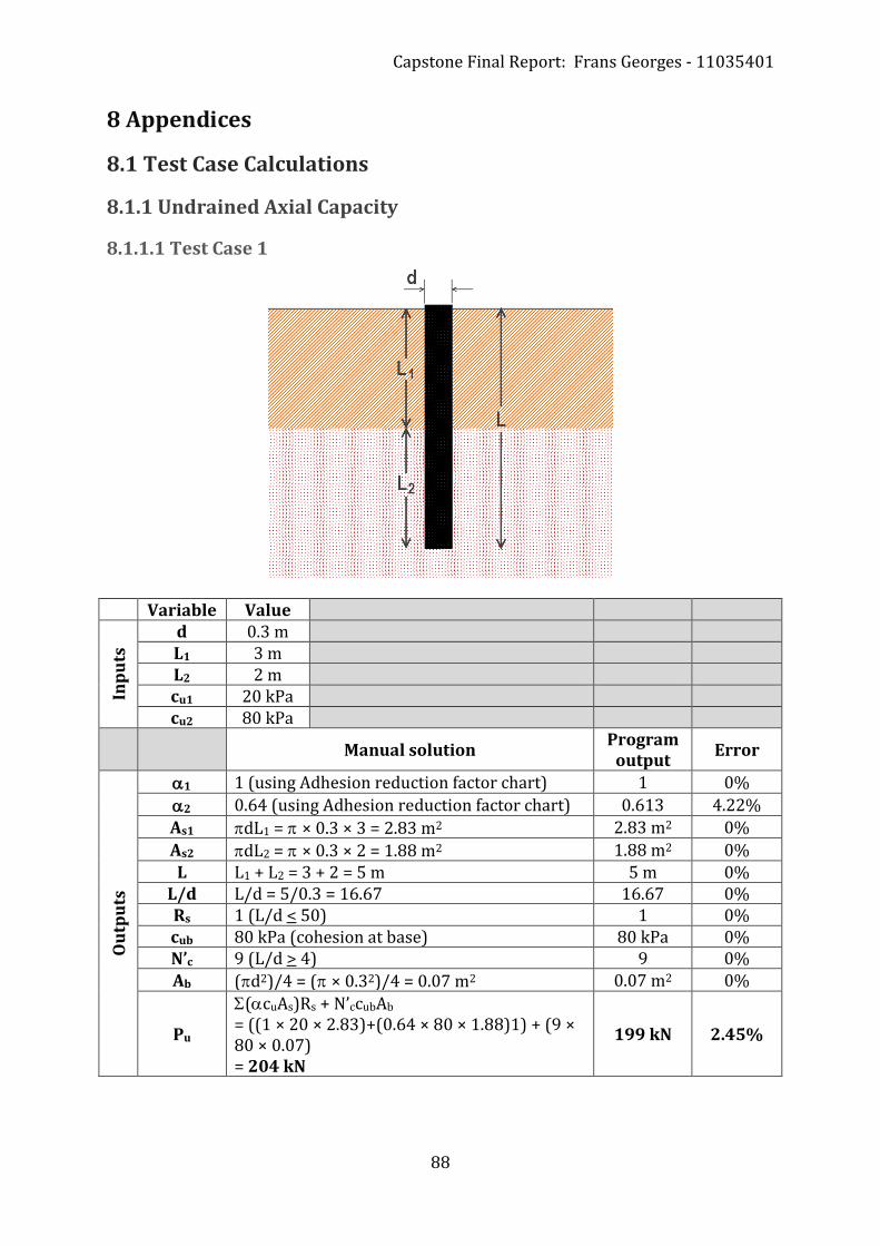
Capstone Final Report: Frans Georges - 11035401
88
8 Appendices
8.1 Test Case Calculations
8.1.1 Undrained Axial Capacity
8.1.1.1 Test Case 1
Variable Value
Inp
uts
d 0.3 m L1 3 m L2 2 m cu1 20 kPa cu2 80 kPa
Manual solution Program
output Error
Ou
tpu
ts
1 1 (using Adhesion reduction factor chart) 1 0%
2 0.64 (using Adhesion reduction factor chart) 0.613 4.22%
As1 dL1 = × 0.3 × 3 = 2.83 m2 2.83 m2 0%
As2 dL2 = × 0.3 × 2 = 1.88 m2 1.88 m2 0% L L1 + L2 = 3 + 2 = 5 m 5 m 0%
L/d L/d = 5/0.3 = 16.67 16.67 0% Rs 1 (L/d < 50) 1 0% cub 80 kPa (cohesion at base) 80 kPa 0% N’c 9 (L/d > 4) 9 0% Ab (d2)/4 = (× 0.32)/4 = 0.07 m2 0.07 m2 0%
Pu
(cuAs)Rs + N’ccubAb
= ((1 × 20 × 2.83)+(0.64 × 80 × 1.88)1) + (9 × 80 × 0.07) = 204 kN
199 kN 2.45%
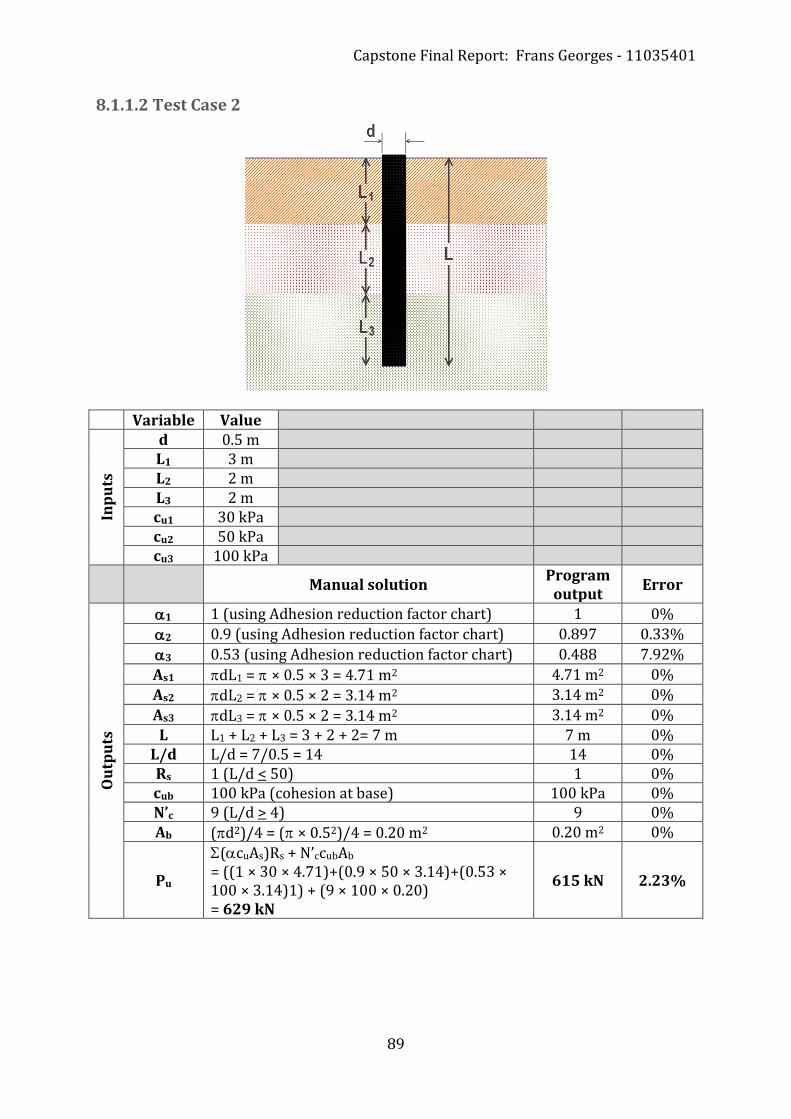
Capstone Final Report: Frans Georges - 11035401
89
8.1.1.2 Test Case 2
Variable Value
Inp
uts
d 0.5 m L1 3 m L2 2 m L3 2 m cu1 30 kPa cu2 50 kPa cu3 100 kPa
Manual solution Program
output Error
Ou
tpu
ts
1 1 (using Adhesion reduction factor chart) 1 0%
2 0.9 (using Adhesion reduction factor chart) 0.897 0.33%
3 0.53 (using Adhesion reduction factor chart) 0.488 7.92%
As1 dL1 = × 0.5 × 3 = 4.71 m2 4.71 m2 0%
As2 dL2 = × 0.5 × 2 = 3.14 m2 3.14 m2 0%
As3 dL3 = × 0.5 × 2 = 3.14 m2 3.14 m2 0%
L L1 + L2 + L3 = 3 + 2 + 2= 7 m 7 m 0% L/d L/d = 7/0.5 = 14 14 0% Rs 1 (L/d < 50) 1 0% cub 100 kPa (cohesion at base) 100 kPa 0% N’c 9 (L/d > 4) 9 0% Ab (d2)/4 = (× 0.52)/4 = 0.20 m2 0.20 m2 0%
Pu
(cuAs)Rs + N’ccubAb
= ((1 × 30 × 4.71)+(0.9 × 50 × 3.14)+(0.53 × 100 × 3.14)1) + (9 × 100 × 0.20) = 629 kN
615 kN 2.23%

Capstone Final Report: Frans Georges - 11035401
90
8.1.1.3 Test Case 3
Variable Value
Inp
uts
d 0.4 m L1 3 m L2 2 m L3 2 m L4 3 m L5 1 m cu1 25 kPa cu2 50 kPa cu3 60 kPa cu4 90 kPa cu5 120 kPa
Manual solution Program
output Error
Ou
tpu
ts
1 1 (using Adhesion reduction factor chart) 1 0%
2 0.9 (using Adhesion reduction factor chart) 0.897 0.33%
3 0.78 (using Adhesion reduction factor chart) 0.789 1.15%
4 0.57 (using Adhesion reduction factor chart) 0.545 4.39%
5 0.44 (using Adhesion reduction factor chart) 0.402 8.64%
As1 dL1 = × 0.4 × 3 = 3.77 m2 3.77 m2 0%
As2 dL2 = × 0.4 × 2 = 2.51 m2 2.51 m2 0%
As3 dL3 = × 0.4 × 2 = 2.51 m2 2.51 m2 0%
As4 dL4 = × 0.4 × 3 = 3.77 m2 3.77 m2 0%
As5 dL5 = × 0.4 × 1 = 1.26 m2 1.26 m2 0% L L1 + L2 + L3 + L4 + L5 = 3 + 2 + 2 + 3 + 1 = 11 m 11 m 0%
L/d L/d = 11/0.4 = 27.5 27.5 0% Rs 1 (L/d < 50) 1 0% cub 120 kPa (cohesion at base) 120 kPa 0% N’c 9 (L/d > 4) 9 0% Ab (d2)/4 = (× 0.42)/4 = 0.13 m2 0.13 m2 0%
Pu
(cuAs)Rs + N’ccubAb
= ((1 × 25 × 3.77)+(0.9 × 50 × 2.51)+(0.78 × 60 × 2.51)+ (0.57 × 90 × 3.77)+ (0.44 × 120 × 1.26)1) + (9 × 120 × 0.13) = 725 kN
712 kN 1.79%

Capstone Final Report: Frans Georges - 11035401
91
8.1.2 Drained Axial Capacity
8.1.2.1 Test Case 1
Variable Value
Note: Problem is split into two layers due to the water table In
pu
ts d 0.5 m
wtd 1m L1 11 m Medium density sand
1 18 kN/m3 Driven pile
Manual solution Program
output Error
Ou
tpu
ts
L1 1 m 1 m 0% L2 10 m 10 m 0%
1 18 kN/m3 (stays the same; above water table) 18 kN/m3 0%
2 (18 – 9.8) = 8.2 kN/m3 8.2 kN/m3 0%
As1 dL1 = × 0.5 × 1 = 1.5708 m2 1.5708 m2 0%
As2 dL2 = × 0.5 × 10 = 15.708 m2 15.708 m2 0%
top1 0 kPa 0 kPa 0%
bot1 1L1 = 18 × 1 = 18 kPa 18 kPa 0%
top2 = bot1 = 18 kPa 18 kPa 0%
bot2 top2 + (2L2) = 18 + (8.2 × 10) = 100 kPa 100 kPa 0% F 1 (Medium Density, Driven Pile) 1 0%
Nq 100 (Medium Density, Driven Pile) 100 0%
’vb 100 kPa (stress at base) 100 kPa 0%
Ab (d2)/4 = (× 0.52)/4 = 0.1963 m2 0.1963 m2 0%
Pu
F(’vAs) + Nq’vbAb
= 1(((0+18)/2 × 1.5708) + ((18+100)/2 × 15.708)) + (100 × 100 × 0.1963) = 2904 kN
2904 kN 0%

Capstone Final Report: Frans Georges - 11035401
92
8.1.2.2 Test Case 2
Variable Value
Note: Problem is split into three layers due to the water table in the second layer In
pu
ts
d 0.5 m wtd 6 m L1 4 m L2 3 m
1 17 kN/m3 Dense sand
2 20 kN/m3 Driven pile
Manual solution Program
output Error
Ou
tpu
ts
L1 4 m 4 m 0% L2 2 m 2 m 0% L3 1 m 1 m 0%
1 17 kN/m3 (stays the same; above water table) 17 kN/m3 0%
2 20 kN/m3 (stays the same; above water table) 20 kN/m3 0%
3 (20 – 9.8) = 10.2 kN/m3 10.2 kN/m3 0%
As1 dL1 = × 0.5 × 4 = 6.2832 m2 6.2832 m2 0%
As2 dL2 = × 0.5 × 2 = 3.1416 m2 3.1416 m2 0%
As3 dL3 = × 0.5 × 1 = 1.5708 m2 1.5708 m2 0%
top1 0 kPa 0 kPa 0%
bot1 1L1 = 17 × 4 = 68 kPa 68 kPa 0%
top2 = bot1 = 68 kPa 68 kPa 0%
bot2 top2 + (2L2) = 68 + (20 × 2) = 108 kPa 108 kPa 0%
top3 = bot2 = 108 kPa 108 kPa 0%
bot3 top3 + (3L3) = 108 + (10.2 × 1) = 118.2 kPa 118.2 kPa 0% F 1.5 (Dense soil, Driven Pile) 1.5 0%
Nq 180 (Dense soil, Driven Pile) 180 0%
’vb 118.2 kPa (stress at base) 118.2 kPa 0%
Ab (d2)/4 = (× 0.52)/4 = 0.1963 m2 0.1963 m2 0%
Pu
F(’vAs) + Nq’vbAb
= 1.5(((0+68)/2 × 6.2832)+((68+108)/2 × 3.1416)+((108+118.2)/2 × 1.5708)) + (180 × 118.2 × 0.1963) = 5178 kN
5178 kN 0%

Capstone Final Report: Frans Georges - 11035401
93
8.1.2.3 Test Case 3
Variable Value
Note: No splitting of layers is required for this test case, as the water table is at the interface of Layers 1 and 2.
Inp
uts
d 0.6 m wtd 2 m L1 2 m L2 4 m L3 3 m
1 16 kN/m3
2 19 kN/m3 Loose sand
3 22 kN/m3 Bored pile
Manual solution Program
output Error
Ou
tpu
ts
1 16 kN/m3 (stays the same; above water table) 16 kN/m3 0%
2 (19 – 9.8) = 9.2 kN/m3 9.2 kN/m3 0%
3 (22 – 9.8) = 12.2 kN/m3 12.2 kN/m3 0%
As1 dL1 = × 0.6 × 2 = 3.7699 m2 3.7699 m2 0%
As2 dL2 = × 0.6 × 4 = 7.5398 m2 7.5398 m2 0%
As3 dL3 = × 0.6 × 3 = 5.6549 m2 5.6549 m2 0%
top1 0 kPa 0 kPa 0%
bot1 1L1 = 16 × 2 = 32 kPa 32 kPa 0%
top2 = bot1 = 32 kPa 32 kPa 0%
bot2 top2 + (2L2) = 32 + (9.2 × 4) = 68.8 kPa 68.8 kPa 0%
top3 = bot2 = 68.8 kPa 68.8 kPa 0%
bot3 top3 + (3L3) = 68.8 + (12.2 × 3) = 105.4 kPa 105.4 kPa 0% F 0.3 (Loose soil, Bored Pile) 0.3 0%
Nq 25 (Loose soil, Bored Pile) 25 0%
’vb 105.4 kPa (stress at base) 105.4 kPa 0%
Ab (d2)/4 = (× 0.62)/4 = 0.2827 m2 0.2827 m2 0%
Pu
F(’vAs) + Nq’vbAb
= 0.3(((0+32)/2 × 3.7699)+((32+68.8)/2 × 7.5398)+((68.8+105.4)/2 × 5.6549)) + (25 × 105.4 × 0.2827) = 1025 kN
1025 kN 0%

Capstone Final Report: Frans Georges - 11035401
94
8.1.3 Hybrid Axial Capacity
8.1.3.1 Test Case 1
Variable Value
Note: The test case will be split into three layers due to the water table being in the first layer. In
pu
ts
d 0.3 m wtd 1 m L1 3 m L2 3 m
1 16 kN/m3 Layer 1 is clay
2 20 kN/m3 Layer 2 is Medium density sand cu1 60 kPa Bored pile
Manual solution Program
output Error
Ou
tpu
ts
L1 1 m 1 m 0% L2 2 m 2 m 0% L3 3 m 3 m 0%
1 16 kN/m3 (stays the same; above water table) 16 kN/m3 0%
2 (16 – 9.8) = 6.2 kN/m3 6.2 kN/m3 0%
3 (20 – 9.8) = 10.2 kN/m3 10.2 kN/m3 0%
As1 dL1 = × 0.3 × 1 = 0.9425 m2 0.9425 m2 0%
As2 dL2 = × 0.3 × 2 = 1.885 m2 1.885 m2 0%
As3 dL3 = × 0.3 × 3 = 2.8274 m2 2.8274 m2 0%
top1 0 kPa 0 kPa 0%
bot1 1L1 = 16 × 1 = 16 kPa 16 kPa 0%
top2 = bot1 = 16 kPa 16 kPa 0%
bot2 top2 + (2L2) = 16 + (6.2 × 2) = 28.4 kPa 28.4 kPa 0%
top3 = bot2 = 28.4 kPa 28.4 kPa 0%
bot3 top3 + (3L3) = 28.4 + (10.2 × 3) = 59 kPa 59 kPa 0%
1 0.78 (using Adhesion reduction factor chart) 0.789 1.15%

Capstone Final Report: Frans Georges - 11035401
95
2 0.78 (using Adhesion reduction factor chart) 0.789 1.15% L L1 + L2 + L3 = 1 + 2 + 3 = 6 m 6 m 0%
L/d L/d = 6/0.3 = 20 20 0% Rs 1 (L/d < 50) 1 0% N’c 9 (L/d > 4) 9 0% F 0.5 (Medium density, Cast In-Situ Pile) 0.5 0%
Nq 60 (Medium density, Cast In-Situ Pile) 60 0%
’vb 59 kPa (stress at base) 59 kPa 0%
Ab (d2)/4 = (× 0.32)/4 = 0.0707 m2 0.0707 m2 0%
Ps1 Rs1cu1As1 = 1 × 0.78 × 60 × 0.9425 = 43.99 kN 44.62 kN 1.43%
Ps2 Rs2cu2As2 = 1 × 0.78 × 60 × 1.885 = 87.98 kN 89.24 kN 1.43%
Ps3 F’vAs3 = 0.5 × (28.4+59)/2 × 2.8274 = 61.78 kN 61.78 kN 0%
Pb Nq’vbAb = 60 × 59 × 0.0707 = 250.3 kN 250.3 kN 0%
Pu
Ps1 + Ps2 + Ps3 + Pb
= 43.99 + 87.98 + 61.78 + 250.3 = 444 kN
446 kN 0.45%

Capstone Final Report: Frans Georges - 11035401
96
8.1.3.2 Test Case 2
Variable Value
Note: The test case will be split into four layers due to the water table being in the first layer. In
pu
ts
d 0.6 m wtd 2 m L1 4 m L2 2 m L3 2 m
1 16 kN/m3
2 21 kN/m3
3 19 kN/m3 Layers 1 and 3 are clay cu1 30 kPa Layer 2 is Dense sand cu3 120 kPa Cast In-Situ pile
Manual solution Program
output Error
Ou
tpu
ts
L1 2 m 2 m 0% L2 2 m 2 m 0% L3 2 m 2 m 0% L4 2 m 2 m 0%
1 16 kN/m3 (stays the same; above water table) 16 kN/m3 0%
2 (16 – 9.8) = 6.2 kN/m3 6.2 kN/m3 0%
3 (21 – 9.8) = 11.2 kN/m3 11.2 kN/m3 0%
4 (19 – 9.8) = 9.2 kN/m3 9.2 kN/m3 0%
As1 dL1 = × 0.6 × 2 = 3.7699 m2 3.7699 m2 0%
As2 dL2 = × 0.6 × 2 = 3.7699 m2 3.7699 m2 0%
As3 dL3 = × 0.6 × 2 = 3.7699 m2 3.7699 m2 0%
As4 dL4 = × 0.6 × 2 = 3.7699 m2 3.7699 m2 0%
top1 0 kPa 0 kPa 0%
bot1 1L1 = 16 × 2 = 32 kPa 32 kPa 0%
top2 = bot1 = 32 kPa 32 kPa 0%
bot2 top2 + (2L2) = 32 + (6.2 × 2) = 44.4 kPa 44.4 kPa 0%

Capstone Final Report: Frans Georges - 11035401
97
top3 = bot2 = 44.4 kPa 44.4 kPa 0%
bot3 top3 + (3L3) = 44.4 + (11.2 × 2) = 66.8 kPa 66.8 kPa 0%
top4 = bot3 = 66.8 kPa 66.8 kPa 0%
bot4 top3 + (4L4) = 66.8 + (9.2 × 2) = 85.2 kPa 85.2 kPa 0%
1 1 (using Adhesion reduction factor chart) 1 0%
2 1 (using Adhesion reduction factor chart) 1 0%
4 0.45 (using Adhesion reduction factor chart) 0.402 10.67% L L1 + L2 + L3 + L4 = 2 + 2 + 2 + 2 = 8 m 8 m 0%
L/d L/d = 8/0.6 = 13.33 13.33 0% Rs 1 (L/d < 50) 1 0% N’c 9 (L/d > 4) 9 0% F 0.8 (Dense sand, Cast In-Situ Pile) 0.8 0%
Nq 100 (Dense sand, Cast In-Situ Pile) 100 0% cub 120 kPa (cohesion at base) 120 kPa 0% Ab (d2)/4 = (× 0.62)/4 = 0.2827 m2 0.2827 m2 0%
Ps1 Rs1cu1As1 = 1 × 1 × 30 × 3.7699 = 113.1 kN 113.1 kN 0%
Ps2 Rs2cu2As2 = 1 × 1 × 30 × 3.7699 = 113.1 kN 113.1 kN 0%
Ps3 F’vAs3 = 0.8 × (44.4+66.8)/2 × 3.7699 = 167.69 kN
167.69 kN 0%
Ps4 Rs4cu4As4 = 1 × 0.45 × 120 × 3.7699 = 203.58 kN
181.86 kN 10.67%
Pb N’ccubAb = 9 × 120 × 0.2827 = 305.3 kN 305.3 kN 0%
Pu
Ps1 + Ps2 + Ps3 + Ps4 + Pb
= 113.1 + 113.1 + 167.69 + 203.58 + 305.3 = 903 kN
881 kN 2.44%

Capstone Final Report: Frans Georges - 11035401
98
8.1.4 Free-Head Lateral Capacity (Cohesive Soils)
8.1.4.1 Test Case 1
Variable Value
Inp
uts
d 0.5 m L 8 m e 0.5 m cu 50 kPa My 700 kNm
Manual solution Program
output Error
Ou
tpu
ts
L/d L/d = 8/0.5 = 16 16 0% e/d e/d = 0.5/0.5 = 1 1 0%
S 44 (using Free-headed, cohesive soil FM1 chart) 43.4 1.36%
Hu1 Scud2 = 44 × 50 × 0.52 = 550 kN 542.5 kN 1.36% f Hu1/9cud = 550/(9 × 50 × 0.5) = 2.444 2.411 1.35% g L – f – 1.5d = 8 – 2.444 – (1.5 × 0.5) = 4.806 4.839 0.69%
Mmax1 (9/4)cudg2 = (9/4) × 50 × 0.5 × 4.8062 = 1299.2 kNm
1317.1 kNm 1.38%
L 9(-(e/d +1.5) + ((e/d + 1.5)2 + (2My/9cud3))0.5) = 9(-2.5 + (2.52 + (1400/9 × 50 × 0.53))0.5) = 27.7
27.7 0%
Hu2 Lcud2 = 27.7 × 50 × 0.52 = 346.2 kN 346.2 kN 0% Mmax2 = My = 700 kNm 700 kNm 0%
FM Failure Mode 2 Failure Mode 2
Hu As FM2 governs, Hu = Hu2 = 346 kN 346 kN 0% Mmax As FM2 governs, Mmax = Mmax2 = 700 kNm 700 kNm 0%

Capstone Final Report: Frans Georges - 11035401
99
8.1.4.2 Test Case 2
Variable Value
Inp
uts
d 0.3 m L 4.5 m e 1.5 m cu 60 kPa My 650 kNm
Manual solution Program
output Error
Ou
tpu
ts
L/d L/d = 4.5/0.3 = 15 15 0% e/d e/d = 1.5/0.3 = 5 5 0%
S 34 (using Free-headed, cohesive soil FM1 chart) 27.7 18.53%
Hu1 Scud2 = 34 × 60 × 0.32 = 183.6 kN 149.6 kN 18.52% f Hu1/9cud = 183.6/(9 × 60 × 0.3) = 1.133 0.923 18.56% g L – f – 1.5d = 4.5 – 1.133 – (1.5 × 0.3) = 2.917 3.127 7.2%
Mmax1 (9/4)cudg2 = (9/4) × 60 × 0.3 × 2.9172 = 345 kNm
396 kNm 14.78%
L 9(-(e/d +1.5) + ((e/d + 1.5)2 + (2My/9cud3))0.5) = 9(-6.5 + (6.52 + (1300/9 × 60 × 0.33))0.5) = 44.7
44.7 0%
Hu2 Lcud2 = 44.7 × 60 × 0.32 = 241.2 kN 241.4 kN 0.08% Mmax2 = My = 650 kNm 650 kNm 0%
FM Failure Mode 1 Failure Mode 1
Hu As FM1 governs, Hu = Hu1 = 184 kN 150 kN 18.48% Mmax As FM1 governs, Mmax = Mmax1 = 345 kNm 396 kNm 14.78%

Capstone Final Report: Frans Georges - 11035401
100
8.1.5 Fixed-Head Lateral Capacity (Cohesive Soils)
8.1.5.1 Test Case 1
Variable Value
Inp
uts
d 0.5 m L 8 m cu 50 kPa My 700 kNm
Manual solution Program
output Error
Ou
tpu
ts
Hu1 9cud(L – 1.5d) = 9 × 50 × 0.5 × (8 – 0.75) = 1631 kN
1631 kN 0%
Mmax1 (Hu1(L + 1.5d)/2 = (1631 × (8 + 0.75))/2 = 7137 kNm
7137 kNm 0%
g 2L – 0.5((16My/9cud) + 8L2 + 18d2)0.5 = 16 – 0.5((11200/225) + 512 + 4.5)0.5 = 4.102
4.102 0%
f L – 1.5d – g = 8 – 0.75 – 4.102 = 3.148 3.148 0% Hu2 9cufd = 9 × 50 × 3.148 × 0.5 = 708 kN 708 kN 0%
Mmax2 (Hu2(f + 3d))/2 – My = (708(3.148 + 1.5))/2 – 700 = 946 kNm
946 kNm 0%
Hu3 (Obtain coefficient using Free-headed, cohesive soil FM2 chart, restrained solution) = 55 Hu2 = 55 × cud2 = 55 × 50 × 0.52 = 688 kN
682 kN 0.87%
Mmax3 = My = 700 kNm 700 kNm 0%
FM Failure Mode 3 Failure Mode 3
Hu As FM3 governs, Hu = Hu3 = 688 kN 682 kN 0.87% Mmax As FM3 governs, Mmax = Mmax3 = 700 kNm 700 kNm 0%
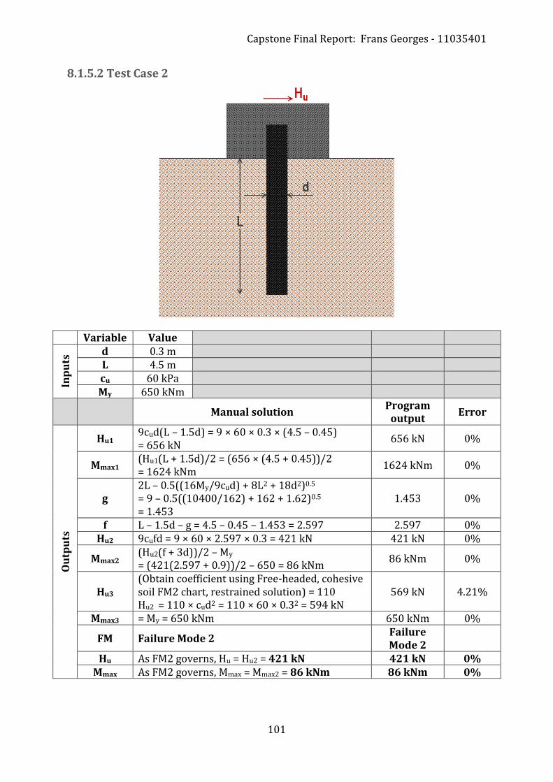
Capstone Final Report: Frans Georges - 11035401
101
8.1.5.2 Test Case 2
Variable Value
Inp
uts
d 0.3 m L 4.5 m cu 60 kPa My 650 kNm
Manual solution Program
output Error
Ou
tpu
ts
Hu1 9cud(L – 1.5d) = 9 × 60 × 0.3 × (4.5 – 0.45) = 656 kN
656 kN 0%
Mmax1 (Hu1(L + 1.5d)/2 = (656 × (4.5 + 0.45))/2 = 1624 kNm
1624 kNm 0%
g 2L – 0.5((16My/9cud) + 8L2 + 18d2)0.5 = 9 – 0.5((10400/162) + 162 + 1.62)0.5 = 1.453
1.453 0%
f L – 1.5d – g = 4.5 – 0.45 – 1.453 = 2.597 2.597 0% Hu2 9cufd = 9 × 60 × 2.597 × 0.3 = 421 kN 421 kN 0%
Mmax2 (Hu2(f + 3d))/2 – My = (421(2.597 + 0.9))/2 – 650 = 86 kNm
86 kNm 0%
Hu3 (Obtain coefficient using Free-headed, cohesive soil FM2 chart, restrained solution) = 110 Hu2 = 110 × cud2 = 110 × 60 × 0.32 = 594 kN
569 kN 4.21%
Mmax3 = My = 650 kNm 650 kNm 0%
FM Failure Mode 2 Failure Mode 2
Hu As FM2 governs, Hu = Hu2 = 421 kN 421 kN 0% Mmax As FM2 governs, Mmax = Mmax2 = 86 kNm 86 kNm 0%

Capstone Final Report: Frans Georges - 11035401
102
8.1.6 Free-Head Lateral Capacity (Cohesionless Soils)
8.1.6.1 Test Case 1
Variable Value
Inp
uts
d 0.5 m L 8 m e 0.5 m
18 kN/m3
My 700 kNm
30o
Manual solution Program
output Error
Ou
tpu
ts
’v L = 18 × 8 = 144 kPa 144 kPa 0% e/d e/d = 0.5/0.5 = 1 1 0% Kp tan2(45 + /2) = tan2(45 + 15) = 3 3 0%
Hu1 (’vKpdL2)/(2(e + L)) = (144 × 3 × 0.5 × 82)/(2(0.5 + 8)) = 813 kN
813 kN 0%
f (L3/(3(e + L)))0.5 = (83/(3(0.5 + 8)))0.5 = 4.48 4.48 0%
Mmax1 Hu1 (e + (2f/3)) = 813 (0.5 + ((2 × 4.48)/3)) = 2835 kNm
2835 kNm 0%
x x-axis on FM2 chart for cohesionless soil My/(Kpd4) = 700/(3 × 18 × 0.54) = 207
207 0%
y Value on y-axis, from using the value of x on the same chart = 70
74 5.71%
Hu2 yKpd3 = 70 × 3 × 18 × 0.53 = 473 kN 502 kN 6.13% Mmax2 = My = 700 kNm 700 kNm 0%
FM Failure Mode 2 Failure Mode 2
Hu As FM2 governs, Hu = Hu2 = 473 kN 502 kN 6.13% Mmax As FM2 governs, Mmax = Mmax2 = 700 kNm 700 kNm 0%

Capstone Final Report: Frans Georges - 11035401
103
8.1.6.2 Test Case 2
Variable Value
Inp
uts
d 0.3 m L 4.5 m e 1.5 m
20 kN/m3
My 650 kNm
30o
Manual solution Program
output Error
Ou
tpu
ts
’v L = 20 × 4.5 = 90 kPa 90 kPa 0% e/d e/d = 1.5/0.3 = 5 5 0% Kp tan2(45 + /2) = tan2(45 + 15) = 3 3 0%
Hu1 (’vKpdL2)/(2(e + L)) = (90 × 3 × 0.3 × 4.52)/(2(1.5 + 4.5)) = 137 kN
137 kN 0%
f (L3/(3(e + L)))0.5 = (4.53/(3(1.5 + 4.5)))0.5 = 2.25
2.25 0%
Mmax1 Hu1 (e + (2f/3)) = 137 (1.5 + ((2 × 2.25)/3)) = 410 kNm
410 kNm 0%
x x-axis on FM2 chart for cohesionless soil My/(Kpd4) = 650/(3 × 20 × 0.34) = 1337
1337 0%
y Value on y-axis, from using the value of x on the same chart = 170
164 3.53%
Hu2 yKpd3 = 170 × 3 × 18 × 0.53 = 275 kN 266 kN 3.27% Mmax2 = My = 650 kNm 650 kNm 0%
FM Failure Mode 1 Failure Mode 1
Hu As FM1 governs, Hu = Hu1 = 137 kN 137 kN 0% Mmax As FM1 governs, Mmax = Mmax1 = 410 kNm 410 kNm 0%

Capstone Final Report: Frans Georges - 11035401
104
8.1.7 Fixed-Head Lateral Capacity (Cohesionless Soils)
8.1.7.1 Test Case 1
Variable Value
Inp
uts
d 0.5 m L 8 m
18 kN/m3
My 700 kNm
30o
Manual solution Program
output Error
’v L = 18 × 8 = 144 kPa 144 kPa 0%
Kp tan2(45 + /2) = tan2(45 + 15) = 3 3 0%
Hu1 1.5’vKpdL = 1.5 × 144 × 3 × 0.5 × 8 = 2592 kN 2592 kN 0% Mmax1 (2Hu1L)/3 = (2 × 2592 × 8)/3 = 13824 kNm 13824 kNm 0%
Hu2 ((0.5’vdL2Kp) + My)/L = ((0.5 × 144 × 0.5 × 64 × 3) + 700)/8 = 952 kN
952 kN 0%
f (2Hu2/(3dKp))0.5 = (2 × 952/(3 × 18 × 0.5 × 3))0.5 = 4.85
4.85 0%
Mmax2 ((2Hu2f)/3) – My = ((2 × 952 × 4.85)/3) – 700 = 2378 kNm
2378 kNm 0%
x x-axis on free-headed pile FM2 chart for cohesionless soil (using restrained solution) My/(Kpd4) = 700/(3 × 18 × 0.54) = 207
207 0%
y Value on y-axis, from using the value of x on the same chart = 120
117 0.025%
Hu3 yKpd3 = 120 × 3 × 18 × 0.53 = 810 kN 790 kN 2.47%
Mmax3 = My = 700 kNm 700 kNm 0%
FM Failure Mode 3 Failure Mode 3
Hu As FM3 governs, Hu = Hu3 = 810 kN 790 kN 2.47% Mmax As FM3 governs, Mmax = Mmax3 = 700 kNm 700 kNm 0%

Capstone Final Report: Frans Georges - 11035401
105
8.1.7.2 Test Case 2
Variable Value
Inp
uts
d 0.3 m L 4.5 m
20 kN/m3
My 650 kNm
30o
Manual solution Program
output Error
’v L = 20 × 4.5 = 90 kPa 90 kPa 0%
Kp tan2(45 + /2) = tan2(45 + 15) = 3 3 0%
Hu1 1.5’vKpdL = 1.5 × 90 × 3 × 0.3 × 4.5 = 547 kN 547 kN 0% Mmax1 (2Hu1L)/3 = (2 × 547 × 4.5)/3 = 1641 kNm 1641 kNm 0%
Hu2 ((0.5’vdL2Kp) + My)/L = ((0.5 × 90 × 0.3 × 4.52 × 3) + 650)/4.5 = 327 kN
327 kN 0%
f (2Hu2/(3dKp))0.5 = (2 × 327/(3 × 20 × 0.3 × 3))0.5 = 3.48
3.48 0%
Mmax2 ((2Hu2f)/3) – My = ((2 × 327 × 3.48)/3) – 650 = 109 kNm
109 kNm 0%
x x-axis on free-headed pile FM2 chart for cohesionless soil (using restrained solution) My/(Kpd4) = 650/(3 × 20 × 0.34) = 1337
1337 0%
y Value on y-axis, from using the value of x on the same chart = 350
345 1.43%
Hu3 yKpd3 = 350 × 3 × 20 × 0.33 = 567 kN 559 kN 1.41% Mmax3 = My = 650 kNm 650 kNm 0%
FM Failure Mode 2 Failure Mode 2
Hu As FM2 governs, Hu = Hu2 = 327 kN 327 kN 0% Mmax As FM2 governs, Mmax = Mmax2 = 109 kNm 109 kNm 0%

Capstone Final Report: Frans Georges - 11035401
106
8.1.8 Vertical Settlement of a Single Floating Pile
8.1.8.1 Test Case 1
Variable Value
Inp
uts
P 2000 kN L 4 m
dout 0.8 m din 0.4 m ES 200 MPa EP 20000 MPa Hollow pile
Manual solution Program
output Error
Ou
tpu
ts
L/d L/d = 4/0.8 = 5 5 0%
RA Ag = (× 0.82)/4 = 0.503 m2
As = 0.503 – ((× 0.42)/4) = 0.377 m2
RA = As/Ag = 0.377/0.503 = 0.75 0.75 0%
K (EP/ES)RA = (20000/200) × 0.75 = 75 75 0%
I Determine value from Settlement influence factor chart = 1.3
1.37 5.38%
S (P/LES)I = (2000/(4 × 200)) × 1.3 = 3.25 mm 3.4 mm 4.62%

Capstone Final Report: Frans Georges - 11035401
107
8.1.8.2 Test Case 2
Variable Value
Inp
uts
P 5000 kN L 12 m
dout 0.6 m din 0 m ES 300 MPa EP 25000 MPa Solid pile
Manual solution Program
output Error
Ou
tpu
ts
L/d L/d = 12/0.6 = 20 20 0% RA 1 (solid pile) 1 0% K (EP/ES)RA = (25000/300) × 1 = 83.33 83.33 0%
I Determine value from Settlement influence factor chart = 3.1
3.37 8.71%
S (P/LES)I = (5000/(12 × 300)) × 3.1 = 4.31 mm 4.7 mm 9.05%
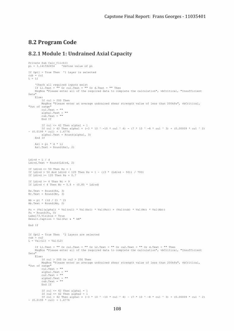
Capstone Final Report: Frans Georges - 11035401
108
8.2 Program Code
8.2.1 Module 1: Undrained Axial Capacity
Private Sub Calc_Click()
pi = 3.141592654 'Define value of pi
If Opt1 = True Then '1 Layer is selected
cub = cu1
L = L1
'Check all required inputs exist
If L1.Text = "" Or cu1.Text = "" Or d.Text = "" Then
MsgBox "Please enter all of the required data to complete the calculation", vbCritical, "Insufficient
Data"
Else:
If cu1 > 200 Then
MsgBox "Please enter an average undrained shear strength value of less than 200kPa", vbCritical,
"Out of range"
cu1.Text = ""
alpha1.Text = ""
cub.Text = ""
End If
If cu1 <= 42 Then alpha1 = 1
If cu1 > 42 Then alpha1 = (-3 * 10 ^ -10 * cu1 ^ 4) - (7 * 10 ^ -8 * cu1 ^ 3) + (0.00009 * cu1 ^ 2)
- (0.0199 * cu1) + 1.6776
alpha1.Text = Round(alpha1, 3)
End If
As1 = pi * d * L1
As1.Text = Round(As1, 2)
Ldivd = L / d
Ldivd.Text = Round(Ldivd, 2)
If Ldivd <= 50 Then Rs = 1
If Ldivd > 50 And Ldivd < 120 Then Rs = 1 - ((3 * (Ldivd - 50)) / 700)
If Ldivd >= 120 Then Rs = 0.7
If Ldivd >= 4 Then Nc = 9
If Ldivd < 4 Then Nc = 5.6 + (0.85 * Ldivd)
Rs.Text = Round(Rs, 3)
Nc.Text = Round(Nc, 3)
Ab = pi * ((d / 2) ^ 2)
Ab.Text = Round(Ab, 2)
Pu = (Val(alpha1) * Val(cu1) * Val(As1) * Val(Rs)) + (Val(cub) * Val(Nc) * Val(Ab))
Pu = Round(Pu, 0)
Label73.Visible = True
Result.Caption = Val(Pu) & " kN"
End If
If Opt2 = True Then '2 Layers are selected
cub = cu2
L = Val(L1) + Val(L2)
If L1.Text = "" Or cu1.Text = "" Or L2.Text = "" Or cu2.Text = "" Or d.Text = "" Then
MsgBox "Please enter all of the required data to complete the calculation", vbCritical, "Insufficient
Data"
Else:
If cu1 > 200 Or cu2 > 200 Then
MsgBox "Please enter an average undrained shear strength value of less than 200kPa", vbCritical,
"Out of range"
cu1.Text = ""
alpha1.Text = ""
cu2.Text = ""
alpha2.Text = ""
cub.Text = ""
End If
If cu1 <= 42 Then alpha1 = 1
If cu2 <= 42 Then alpha2 = 1
If cu1 > 42 Then alpha1 = (-3 * 10 ^ -10 * cu1 ^ 4) - (7 * 10 ^ -8 * cu1 ^ 3) + (0.00009 * cu1 ^ 2)
- (0.0199 * cu1) + 1.6776

Capstone Final Report: Frans Georges - 11035401
109
If cu2 > 42 Then alpha2 = (-3 * 10 ^ -10 * cu2 ^ 4) - (7 * 10 ^ -8 * cu2 ^ 3) + (0.00009 * cu2 ^ 2)
- (0.0199 * cu2) + 1.6776
alpha1.Text = Round(alpha1, 3)
alpha2.Text = Round(alpha2, 3)
End If
As1 = pi * d * L1
As1.Text = Round(As1, 2)
As2 = pi * d * L2
As2.Text = Round(As2, 2)
Ldivd = L / d
Ldivd.Text = Round(Ldivd, 2)
If Ldivd <= 50 Then Rs = 1
If Ldivd > 50 And Ldivd < 120 Then Rs = 1 - ((3 * (Ldivd - 50)) / 700)
If Ldivd >= 120 Then Rs = 0.7
If Ldivd >= 4 Then Nc = 9
If Ldivd < 4 Then Nc = 5.6 + (0.85 * Ldivd)
Rs.Text = Round(Rs, 3)
Nc.Text = Round(Nc, 3)
Ab = pi * ((d / 2) ^ 2)
Ab.Text = Round(Ab, 2)
Pu = (((Val(alpha1) * Val(cu1) * Val(As1)) + (Val(alpha2) * Val(cu2) * Val(As2))) * Val(Rs)) + (Val(cub) *
Val(Nc) * Val(Ab))
Pu = Round(Pu, 0)
Label73.Visible = True
Result.Caption = Val(Pu) & " kN"
End If
If Opt3 = True Then '3 Layers are selected
cub = cu3
L = Val(L1) + Val(L2) + Val(L3)
If L1.Text = "" Or cu1.Text = "" Or L2.Text = "" Or cu2.Text = "" Or L3.Text = "" Or cu3.Text = "" Or
d.Text = "" Then
MsgBox "Please enter all of the required data to complete the calculation", vbCritical, "Insufficient
Data"
Else:
If cu1 > 200 Or cu2 > 200 Or cu3 > 200 Then
MsgBox "Please enter an average undrained shear strength value of less than 200kPa", vbCritical,
"Out of range"
cu1.Text = ""
alpha1.Text = ""
cu2.Text = ""
alpha2.Text = ""
cu3.Text = ""
alpha3.Text = ""
cub.Text = ""
End If
If cu1 <= 42 Then alpha1 = 1
If cu2 <= 42 Then alpha2 = 1
If cu3 <= 42 Then alpha3 = 1
If cu1 > 42 Then alpha1 = (-3 * 10 ^ -10 * cu1 ^ 4) - (7 * 10 ^ -8 * cu1 ^ 3) + (0.00009 * cu1 ^ 2)
- (0.0199 * cu1) + 1.6776
If cu2 > 42 Then alpha2 = (-3 * 10 ^ -10 * cu2 ^ 4) - (7 * 10 ^ -8 * cu2 ^ 3) + (0.00009 * cu2 ^ 2)
- (0.0199 * cu2) + 1.6776
If cu3 > 42 Then alpha3 = (-3 * 10 ^ -10 * cu3 ^ 4) - (7 * 10 ^ -8 * cu3 ^ 3) + (0.00009 * cu3 ^ 2)
- (0.0199 * cu3) + 1.6776
alpha1.Text = Round(alpha1, 3)
alpha2.Text = Round(alpha2, 3)
alpha3.Text = Round(alpha3, 3)
End If
As1 = pi * d * L1
As1.Text = Round(As1, 2)
As2 = pi * d * L2
As2.Text = Round(As2, 2)
As3 = pi * d * L3
As3.Text = Round(As3, 2)
Ldivd = L / d
Ldivd.Text = Round(Ldivd, 2)
If Ldivd <= 50 Then Rs = 1
If Ldivd > 50 And Ldivd < 120 Then Rs = 1 - ((3 * (Ldivd - 50)) / 700)
If Ldivd >= 120 Then Rs = 0.7

Capstone Final Report: Frans Georges - 11035401
110
If Ldivd >= 4 Then Nc = 9
If Ldivd < 4 Then Nc = 5.6 + (0.85 * Ldivd)
Rs.Text = Round(Rs, 3)
Nc.Text = Round(Nc, 3)
Ab = pi * ((d / 2) ^ 2)
Ab.Text = Round(Ab, 2)
Pu = (((Val(alpha1) * Val(cu1) * Val(As1)) + (Val(alpha2) * Val(cu2) * Val(As2)) + (Val(alpha3) * Val(cu3)
* Val(As3))) * Val(Rs)) + (Val(cub) * Val(Nc) * Val(Ab))
Pu = Round(Pu, 0)
Label73.Visible = True
Result.Caption = Val(Pu) & " kN"
End If
If Opt4 = True Then '4 Layers are selected
cub = cu4
L = Val(L1) + Val(L2) + Val(L3) + Val(L4)
If L1.Text = "" Or cu1.Text = "" Or L2.Text = "" Or cu2.Text = "" Or L3.Text = "" Or cu3.Text = "" Or
L4.Text = "" Or cu4.Text = "" Or d.Text = "" Then
MsgBox "Please enter all of the required data to complete the calculation", vbCritical, "Insufficient
Data"
Else:
If cu1 > 200 Or cu2 > 200 Or cu3 > 200 Or cu4 > 200 Then
MsgBox "Please enter an average undrained shear strength value of less than 200kPa", vbCritical,
"Out of range"
cu1.Text = ""
alpha1.Text = ""
cu2.Text = ""
alpha2.Text = ""
cu3.Text = ""
alpha3.Text = ""
cu4.Text = ""
alpha4.Text = ""
cub.Text = ""
End If
If cu1 <= 42 Then alpha1 = 1
If cu2 <= 42 Then alpha2 = 1
If cu3 <= 42 Then alpha3 = 1
If cu4 <= 42 Then alpha4 = 1
If cu1 > 42 Then alpha1 = (-3 * 10 ^ -10 * cu1 ^ 4) - (7 * 10 ^ -8 * cu1 ^ 3) + (0.00009 * cu1 ^ 2)
- (0.0199 * cu1) + 1.6776
If cu2 > 42 Then alpha2 = (-3 * 10 ^ -10 * cu2 ^ 4) - (7 * 10 ^ -8 * cu2 ^ 3) + (0.00009 * cu2 ^ 2)
- (0.0199 * cu2) + 1.6776
If cu3 > 42 Then alpha3 = (-3 * 10 ^ -10 * cu3 ^ 4) - (7 * 10 ^ -8 * cu3 ^ 3) + (0.00009 * cu3 ^ 2)
- (0.0199 * cu3) + 1.6776
If cu4 > 42 Then alpha4 = (-3 * 10 ^ -10 * cu4 ^ 4) - (7 * 10 ^ -8 * cu4 ^ 3) + (0.00009 * cu4 ^ 2)
- (0.0199 * cu4) + 1.6776
alpha1.Text = Round(alpha1, 3)
alpha2.Text = Round(alpha2, 3)
alpha3.Text = Round(alpha3, 3)
alpha4.Text = Round(alpha4, 3)
End If
As1 = pi * d * L1
As1.Text = Round(As1, 2)
As2 = pi * d * L2
As2.Text = Round(As2, 2)
As3 = pi * d * L3
As3.Text = Round(As3, 2)
As4 = pi * d * L4
As4.Text = Round(As4, 2)
Ldivd = L / d
Ldivd.Text = Round(Ldivd, 2)
If Ldivd <= 50 Then Rs = 1
If Ldivd > 50 And Ldivd < 120 Then Rs = 1 - ((3 * (Ldivd - 50)) / 700)
If Ldivd >= 120 Then Rs = 0.7
If Ldivd >= 4 Then Nc = 9
If Ldivd < 4 Then Nc = 5.6 + (0.85 * Ldivd)
Rs.Text = Round(Rs, 3)
Nc.Text = Round(Nc, 3)
Ab = pi * ((d / 2) ^ 2)
Ab.Text = Round(Ab, 2)

Capstone Final Report: Frans Georges - 11035401
111
Pu = (((Val(alpha1) * Val(cu1) * Val(As1)) + (Val(alpha2) * Val(cu2) * Val(As2)) + (Val(alpha3) * Val(cu3)
* Val(As3)) + (Val(alpha4) * Val(cu4) * Val(As4))) * Val(Rs)) + (Val(cub) * Val(Nc) * Val(Ab))
Pu = Round(Pu, 0)
Label73.Visible = True
Result.Caption = Val(Pu) & " kN"
End If
If Opt5 = True Then '5 Layers are selected
cub = cu5
L = Val(L1) + Val(L2) + Val(L3) + Val(L4) + Val(L5)
If L1.Text = "" Or cu1.Text = "" Or L2.Text = "" Or cu2.Text = "" Or L3.Text = "" Or cu3.Text = "" Or
L4.Text = "" Or cu4.Text = "" Or L5.Text = "" Or cu5.Text = "" Or d.Text = "" Then
MsgBox "Please enter all of the required data to complete the calculation", vbCritical, "Insufficient
Data"
Else:
If cu1 > 200 Or cu2 > 200 Or cu3 > 200 Or cu4 > 200 Or cu5 > 200 Then
MsgBox "Please enter an average undrained shear strength value of less than 200kPa", vbCritical,
"Out of range"
cu1.Text = ""
alpha1.Text = ""
cu2.Text = ""
alpha2.Text = ""
cu3.Text = ""
alpha3.Text = ""
cu4.Text = ""
alpha4.Text = ""
cu5.Text = ""
alpha5.Text = ""
cub.Text = ""
End If
If cu1 <= 42 Then alpha1 = 1
If cu2 <= 42 Then alpha2 = 1
If cu3 <= 42 Then alpha3 = 1
If cu4 <= 42 Then alpha4 = 1
If cu5 <= 42 Then alpha5 = 1
If cu1 > 42 Then alpha1 = (-3 * 10 ^ -10 * cu1 ^ 4) - (7 * 10 ^ -8 * cu1 ^ 3) + (0.00009 * cu1 ^ 2)
- (0.0199 * cu1) + 1.6776
If cu2 > 42 Then alpha2 = (-3 * 10 ^ -10 * cu2 ^ 4) - (7 * 10 ^ -8 * cu2 ^ 3) + (0.00009 * cu2 ^ 2)
- (0.0199 * cu2) + 1.6776
If cu3 > 42 Then alpha3 = (-3 * 10 ^ -10 * cu3 ^ 4) - (7 * 10 ^ -8 * cu3 ^ 3) + (0.00009 * cu3 ^ 2)
- (0.0199 * cu3) + 1.6776
If cu4 > 42 Then alpha4 = (-3 * 10 ^ -10 * cu4 ^ 4) - (7 * 10 ^ -8 * cu4 ^ 3) + (0.00009 * cu4 ^ 2)
- (0.0199 * cu4) + 1.6776
If cu5 > 42 Then alpha5 = (-3 * 10 ^ -10 * cu5 ^ 4) - (7 * 10 ^ -8 * cu5 ^ 3) + (0.00009 * cu5 ^ 2)
- (0.0199 * cu5) + 1.6776
alpha1.Text = Round(alpha1, 3)
alpha2.Text = Round(alpha2, 3)
alpha3.Text = Round(alpha3, 3)
alpha4.Text = Round(alpha4, 3)
alpha5.Text = Round(alpha5, 3)
End If
As1 = pi * d * L1
As1.Text = Round(As1, 2)
As2 = pi * d * L2
As2.Text = Round(As2, 2)
As3 = pi * d * L3
As3.Text = Round(As3, 2)
As4 = pi * d * L4
As4.Text = Round(As4, 2)
As5 = pi * d * L5
As5.Text = Round(As5, 2)
Ldivd = L / d
Ldivd.Text = Round(Ldivd, 2)
If Ldivd <= 50 Then Rs = 1
If Ldivd > 50 And Ldivd < 120 Then Rs = 1 - ((3 * (Ldivd - 50)) / 700)
If Ldivd >= 120 Then Rs = 0.7
If Ldivd >= 4 Then Nc = 9
If Ldivd < 4 Then Nc = 5.6 + (0.85 * Ldivd)
Rs.Text = Round(Rs, 3)
Nc.Text = Round(Nc, 3)
Ab = pi * ((d / 2) ^ 2)
Ab.Text = Round(Ab, 2)
Pu = (((Val(alpha1) * Val(cu1) * Val(As1)) + (Val(alpha2) * Val(cu2) * Val(As2)) + (Val(alpha3) * Val(cu3)
* Val(As3)) + (Val(alpha4) * Val(cu4) * Val(As4)) + (Val(alpha5) * Val(cu5) * Val(As5))) * Val(Rs)) +
(Val(cub) * Val(Nc) * Val(Ab))
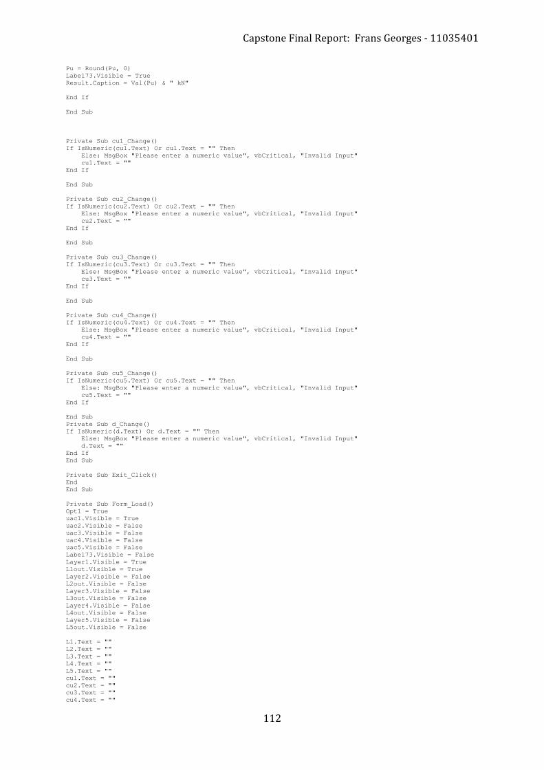
Capstone Final Report: Frans Georges - 11035401
112
Pu = Round(Pu, 0)
Label73.Visible = True
Result.Caption = Val(Pu) & " kN"
End If
End Sub
Private Sub cu1_Change()
If IsNumeric(cu1.Text) Or cu1.Text = "" Then
Else: MsgBox "Please enter a numeric value", vbCritical, "Invalid Input"
cu1.Text = ""
End If
End Sub
Private Sub cu2_Change()
If IsNumeric(cu2.Text) Or cu2.Text = "" Then
Else: MsgBox "Please enter a numeric value", vbCritical, "Invalid Input"
cu2.Text = ""
End If
End Sub
Private Sub cu3_Change()
If IsNumeric(cu3.Text) Or cu3.Text = "" Then
Else: MsgBox "Please enter a numeric value", vbCritical, "Invalid Input"
cu3.Text = ""
End If
End Sub
Private Sub cu4_Change()
If IsNumeric(cu4.Text) Or cu4.Text = "" Then
Else: MsgBox "Please enter a numeric value", vbCritical, "Invalid Input"
cu4.Text = ""
End If
End Sub
Private Sub cu5_Change()
If IsNumeric(cu5.Text) Or cu5.Text = "" Then
Else: MsgBox "Please enter a numeric value", vbCritical, "Invalid Input"
cu5.Text = ""
End If
End Sub
Private Sub d_Change()
If IsNumeric(d.Text) Or d.Text = "" Then
Else: MsgBox "Please enter a numeric value", vbCritical, "Invalid Input"
d.Text = ""
End If
End Sub
Private Sub Exit_Click()
End
End Sub
Private Sub Form_Load()
Opt1 = True
uac1.Visible = True
uac2.Visible = False
uac3.Visible = False
uac4.Visible = False
uac5.Visible = False
Label73.Visible = False
Layer1.Visible = True
L1out.Visible = True
Layer2.Visible = False
L2out.Visible = False
Layer3.Visible = False
L3out.Visible = False
Layer4.Visible = False
L4out.Visible = False
Layer5.Visible = False
L5out.Visible = False
L1.Text = ""
L2.Text = ""
L3.Text = ""
L4.Text = ""
L5.Text = ""
cu1.Text = ""
cu2.Text = ""
cu3.Text = ""
cu4.Text = ""

Capstone Final Report: Frans Georges - 11035401
113
cu5.Text = ""
alpha1.Text = ""
alpha2.Text = ""
alpha3.Text = ""
alpha4.Text = ""
alpha5.Text = ""
As1.Text = ""
As2.Text = ""
As3.Text = ""
As4.Text = ""
As5.Text = ""
L.Text = ""
Ldivd.Text = ""
Rs.Text = ""
cub.Text = ""
Nc.Text = ""
Ab.Text = ""
Result.Caption = ""
d.Text = ""
End Sub
Private Sub L1_Change()
If IsNumeric(L1.Text) Or L1.Text = "" Then
Else: MsgBox "Please enter a numeric value", vbCritical, "Invalid Input"
L1.Text = ""
End If
End Sub
Private Sub L2_Change()
If IsNumeric(L2.Text) Or L2.Text = "" Then
Else: MsgBox "Please enter a numeric value", vbCritical, "Invalid Input"
L2.Text = ""
End If
End Sub
Private Sub L3_Change()
If IsNumeric(L3.Text) Or L3.Text = "" Then
Else: MsgBox "Please enter a numeric value", vbCritical, "Invalid Input"
L3.Text = ""
End If
End Sub
Private Sub L4_Change()
If IsNumeric(L4.Text) Or L4.Text = "" Then
Else: MsgBox "Please enter a numeric value", vbCritical, "Invalid Input"
L4.Text = ""
End If
End Sub
Private Sub L5_Change()
If IsNumeric(L5.Text) Or L5.Text = "" Then
Else: MsgBox "Please enter a numeric value", vbCritical, "Invalid Input"
L5.Text = ""
End If
End Sub
Private Sub Menu_Click()
Title.Show
Title.Top = (Screen.Height - Title.Height) / 2
Title.Left = (Screen.Width - Title.Width) / 2
Unload Me
End Sub
Private Sub mnuAbout_Click()
MsgBox "Program created by Frans Georges for Capstone Project", vbOKOnly, "About"
End Sub
Private Sub Opt1_Click()
uac1.Visible = True
uac2.Visible = False
uac3.Visible = False
uac4.Visible = False
uac5.Visible = False
Label73.Visible = False
Layer1.Visible = True
L1out.Visible = True
Layer2.Visible = False
L2out.Visible = False
Layer3.Visible = False
L3out.Visible = False
Layer4.Visible = False
L4out.Visible = False
Layer5.Visible = False
L5out.Visible = False
L1.Text = ""
L2.Text = ""

Capstone Final Report: Frans Georges - 11035401
114
L3.Text = ""
L4.Text = ""
L5.Text = ""
cu1.Text = ""
cu2.Text = ""
cu3.Text = ""
cu4.Text = ""
cu5.Text = ""
alpha1.Text = ""
alpha2.Text = ""
alpha3.Text = ""
alpha4.Text = ""
alpha5.Text = ""
As1.Text = ""
As2.Text = ""
As3.Text = ""
As4.Text = ""
As5.Text = ""
L.Text = ""
Ldivd.Text = ""
Rs.Text = ""
cub.Text = ""
Nc.Text = ""
Ab.Text = ""
Result.Caption = ""
d.Text = ""
End Sub
Private Sub Opt2_Click()
uac1.Visible = False
uac2.Visible = True
uac3.Visible = False
uac4.Visible = False
uac5.Visible = False
Label73.Visible = False
Layer1.Visible = True
L1out.Visible = True
Layer2.Visible = True
L2out.Visible = True
Layer3.Visible = False
L3out.Visible = False
Layer4.Visible = False
L4out.Visible = False
Layer5.Visible = False
L5out.Visible = False
L1.Text = ""
L2.Text = ""
L3.Text = ""
L4.Text = ""
L5.Text = ""
cu1.Text = ""
cu2.Text = ""
cu3.Text = ""
cu4.Text = ""
cu5.Text = ""
alpha1.Text = ""
alpha2.Text = ""
alpha3.Text = ""
alpha4.Text = ""
alpha5.Text = ""
As1.Text = ""
As2.Text = ""
As3.Text = ""
As4.Text = ""
As5.Text = ""
L.Text = ""
Ldivd.Text = ""
Rs.Text = ""
cub.Text = ""
Nc.Text = ""
Ab.Text = ""
Result.Caption = ""
d.Text = ""
End Sub
Private Sub Opt3_Click()
uac1.Visible = False
uac2.Visible = False
uac3.Visible = True
uac4.Visible = False

Capstone Final Report: Frans Georges - 11035401
115
uac5.Visible = False
Label73.Visible = False
Layer1.Visible = True
L1out.Visible = True
Layer2.Visible = True
L2out.Visible = True
Layer3.Visible = True
L3out.Visible = True
Layer4.Visible = False
L4out.Visible = False
Layer5.Visible = False
L5out.Visible = False
L1.Text = ""
L2.Text = ""
L3.Text = ""
L4.Text = ""
L5.Text = ""
cu1.Text = ""
cu2.Text = ""
cu3.Text = ""
cu4.Text = ""
cu5.Text = ""
alpha1.Text = ""
alpha2.Text = ""
alpha3.Text = ""
alpha4.Text = ""
alpha5.Text = ""
As1.Text = ""
As2.Text = ""
As3.Text = ""
As4.Text = ""
As5.Text = ""
L.Text = ""
Ldivd.Text = ""
Rs.Text = ""
cub.Text = ""
Nc.Text = ""
Ab.Text = ""
Result.Caption = ""
d.Text = ""
End Sub
Private Sub Opt4_Click()
uac1.Visible = False
uac2.Visible = False
uac3.Visible = False
uac4.Visible = True
uac5.Visible = False
Label73.Visible = False
Layer1.Visible = True
L1out.Visible = True
Layer2.Visible = True
L2out.Visible = True
Layer3.Visible = True
L3out.Visible = True
Layer4.Visible = True
L4out.Visible = True
Layer5.Visible = False
L5out.Visible = False
L1.Text = ""
L2.Text = ""
L3.Text = ""
L4.Text = ""
L5.Text = ""
cu1.Text = ""
cu2.Text = ""
cu3.Text = ""
cu4.Text = ""
cu5.Text = ""
alpha1.Text = ""
alpha2.Text = ""
alpha3.Text = ""
alpha4.Text = ""

Capstone Final Report: Frans Georges - 11035401
116
alpha5.Text = ""
As1.Text = ""
As2.Text = ""
As3.Text = ""
As4.Text = ""
As5.Text = ""
L.Text = ""
Ldivd.Text = ""
Rs.Text = ""
cub.Text = ""
Nc.Text = ""
Ab.Text = ""
Result.Caption = ""
d.Text = ""
End Sub
Private Sub Opt5_Click()
uac1.Visible = False
uac2.Visible = False
uac3.Visible = False
uac4.Visible = False
uac5.Visible = True
Label73.Visible = False
Layer1.Visible = True
L1out.Visible = True
Layer2.Visible = True
L2out.Visible = True
Layer3.Visible = True
L3out.Visible = True
Layer4.Visible = True
L4out.Visible = True
Layer5.Visible = True
L5out.Visible = True
L1.Text = ""
L2.Text = ""
L3.Text = ""
L4.Text = ""
L5.Text = ""
cu1.Text = ""
cu2.Text = ""
cu3.Text = ""
cu4.Text = ""
cu5.Text = ""
alpha1.Text = ""
alpha2.Text = ""
alpha3.Text = ""
alpha4.Text = ""
alpha5.Text = ""
As1.Text = ""
As2.Text = ""
As3.Text = ""
As4.Text = ""
As5.Text = ""
L.Text = ""
Ldivd.Text = ""
Rs.Text = ""
cub.Text = ""
Nc.Text = ""
Ab.Text = ""
Result.Caption = ""
d.Text = ""
End Sub
Private Sub Reset_Click()
Opt1 = True
uac1.Visible = True
uac2.Visible = False
uac3.Visible = False
uac4.Visible = False
uac5.Visible = False
Label73.Visible = False
Layer1.Visible = True
L1out.Visible = True
Layer2.Visible = False
L2out.Visible = False
Layer3.Visible = False
L3out.Visible = False

Capstone Final Report: Frans Georges - 11035401
117
Layer4.Visible = False
L4out.Visible = False
Layer5.Visible = False
L5out.Visible = False
L1.Text = ""
L2.Text = ""
L3.Text = ""
L4.Text = ""
L5.Text = ""
cu1.Text = ""
cu2.Text = ""
cu3.Text = ""
cu4.Text = ""
cu5.Text = ""
alpha1.Text = ""
alpha2.Text = ""
alpha3.Text = ""
alpha4.Text = ""
alpha5.Text = ""
As1.Text = ""
As2.Text = ""
As3.Text = ""
As4.Text = ""
As5.Text = ""
L.Text = ""
Ldivd.Text = ""
Rs.Text = ""
cub.Text = ""
Nc.Text = ""
Ab.Text = ""
Result.Caption = ""
d.Text = ""
End Sub

Capstone Final Report: Frans Georges - 11035401
118
8.2.2 Module 2: Drained Axial Capacity
Private Sub CalcDAC_Click()
pi = 3.141592654
'checking for diameter input
If d.Text = "" Then
MsgBox "Please enter a value for the diameter of the pile", vbCritical, "Pile Diameter"
End If
'checking for water table depth input
If wtd.Text = "" Then
MsgBox "Please enter a depth for the water table (If water table does not exist, enter a value larger than
the total depth)", vbCritical, "Water Table"
End If
'checking for soil consistency selection
If optL = False And optM = False And optD = False Then
MsgBox "Please select a soil consistency", vbCritical, "Soil Consistency"
End If
'checking for pile installation method selection
If optDRV = False And optBCI = False Then
MsgBox "Please select a Pile Installation Method", vbCritical, "Pile Installation Method"
End If
'loose soil, driven
If optL = True And optDRV = True Then
f = 0.8
Nq = 60
End If
'loose soil, bored/cast insitu
If optL = True And optBCI = True Then
f = 0.3
Nq = 25
End If
'medium soil, driven
If optM = True And optDRV = True Then
f = 1
Nq = 100
End If
'medium soil, bored/cast insitu
If optM = True And optBCI = True Then
f = 0.5
Nq = 60
End If
'dense soil, driven
If optD = True And optDRV = True Then
f = 1.5
Nq = 180
End If
'dense soil, bored/cast insitu
If optD = True And optBCI = True Then
f = 0.8
Nq = 100
End If
'==========================================================================================================
========
'one soil layer, no water table
If Opt1 = True Then
L = L1(0)
If wtd >= L Then
As1(0) = pi * L1(0) * d
As1(0).Text = Round(As1(0), 4)
sigmatop1 = 0
sigmabot1 = gamma1(0) * L1(0)
sigmavb = sigmabot1
Ab = pi * ((d / 2) ^ 2)
Ab.Text = Round(Ab, 4)
trap1 = 0.5 * L1(0) * (sigmatop1 + sigmabot1)
P_s = f * trap1 * As1(0)
P_b = Nq * sigmavb * Ab
P_u = P_s + P_b
P_u = Round(P_u, 0)
Label41.Visible = True
DACResult.Caption = Val(P_u) & " kN"
End If

Capstone Final Report: Frans Georges - 11035401
119
End If
'==========================================================================================================
========
'one soil layer, with water table at the top
If Opt1 = True And wtd = 0 Then
L = L1(0)
gamma1(0) = gamma1(0) - 9.8
As1(0) = pi * L1(0) * d
As1(0).Text = Round(As1(0), 4)
sigmatop1 = 0
sigmabot1 = gamma1(0) * L1(0)
sigmavb = sigmabot1
Ab = pi * ((d / 2) ^ 2)
Ab.Text = Round(Ab, 4)
trap1 = 0.5 * L1(0) * (sigmatop1 + sigmabot1)
P_s = f * trap1 * As1(0)
P_b = Nq * sigmavb * Ab
P_u = P_s + P_b
P_u = Round(P_u, 0)
Label41.Visible = True
DACResult.Caption = Val(P_u) & " kN"
End If
'==========================================================================================================
========
'one soil layer, with water table
If Opt1 = True And wtd > 0 And wtd < L1(0) Then
Layer2(1).Visible = True
a = L1(0) - wtd
L1(0) = wtd
L2(1) = a
gamma2(1) = gamma1(0) - 9.8
As1(0) = pi * L1(0) * d
As1(0).Text = Round(As1(0), 4)
As2(1) = pi * L2(1) * d
As2(1).Text = Round(As2(1), 4)
sigmatop1 = 0
sigmabot1 = gamma1(0) * L1(0)
sigmatop2(0) = sigmabot1
sigmabot2(0) = sigmatop2(0) + (gamma2(1) * L2(1))
L = Val(L1(0)) + Val(L2(1))
sigmavb = sigmabot2(0)
Ab = pi * ((d / 2) ^ 2)
Ab.Text = Round(Ab, 4)
trap1 = 0.5 * (sigmatop1 + sigmabot1)
trap2 = 0.5 * (Val(sigmatop2(0)) + Val(sigmabot2(0)))
P_s1 = trap1 * As1(0)
P_s2 = trap2 * As2(1)
P_s = f * (P_s1 + P_s2)
P_b = Nq * sigmavb * Ab
P_u = P_s + P_b
P_u = Round(P_u, 0)
Label41.Visible = True
DACResult.Caption = Val(P_u) & " kN"
CalcDAC.Enabled = False
End If
'==========================================================================================================
========
'two soil layers, no water table
If Opt2 = True Then
L = Val(L1(0)) + Val(L2(1))
If wtd >= L Then
As1(0) = pi * L1(0) * d
As1(0).Text = Round(As1(0), 4)
As2(1) = pi * L2(1) * d
As2(1).Text = Round(As2(1), 4)
sigmatop1 = 0
sigmabot1 = gamma1(0) * L1(0)
sigmatop2(0) = sigmabot1
sigmabot2(0) = sigmatop2(0) + (gamma2(1) * L2(1))
sigmavb = sigmabot2(0)
Ab = pi * ((d / 2) ^ 2)

Capstone Final Report: Frans Georges - 11035401
120
Ab.Text = Round(Ab, 4)
trap1 = 0.5 * (sigmatop1 + sigmabot1)
trap2 = 0.5 * (Val(sigmatop2(0)) + Val(sigmabot2(0)))
P_s1 = trap1 * As1(0)
P_s2 = trap2 * As2(1)
P_s = f * (P_s1 + P_s2)
P_b = Nq * sigmavb * Ab
P_u = P_s + P_b
P_u = Round(P_u, 0)
Label41.Visible = True
DACResult.Caption = Val(P_u) & " kN"
End If
End If
'==========================================================================================================
========
'two soil layers with water table at layer depths
If Opt2 = True Then
If wtd = 0 Then
gamma1(0) = gamma1(0) - 9.8
gamma2(1) = gamma2(1) - 9.8
End If
If wtd = L1(0) Then
gamma2(1) = gamma2(1) - 9.8
End If
As1(0) = pi * L1(0) * d
As1(0).Text = Round(As1(0), 4)
As2(1) = pi * L2(1) * d
As2(1).Text = Round(As2(1), 4)
sigmatop1 = 0
sigmabot1 = gamma1(0) * L1(0)
sigmatop2(0) = sigmabot1
sigmabot2(0) = sigmatop2(0) + (gamma2(1) * L2(1))
L = Val(L1(0)) + Val(L2(1))
sigmavb = sigmabot2(0)
Ab = pi * ((d / 2) ^ 2)
Ab.Text = Round(Ab, 4)
trap1 = 0.5 * (sigmatop1 + sigmabot1)
trap2 = 0.5 * (Val(sigmatop2(0)) + Val(sigmabot2(0)))
P_s1 = trap1 * As1(0)
P_s2 = trap2 * As2(1)
P_s = f * (P_s1 + P_s2)
P_b = Nq * sigmavb * Ab
P_u = P_s + P_b
P_u = Round(P_u, 0)
Label41.Visible = True
DACResult.Caption = Val(P_u) & " kN"
CalcDAC.Enabled = False
End If
'==========================================================================================================
========
'two soil layers, with water table
If Opt2 = True Then
L = Val(L1(0)) + Val(L2(1))
If wtd > 0 And wtd <> L1(0) And wtd < L Then
Layer3(0).Visible = True
If wtd < L1(0) Then
a = L1(0) - wtd
L3(2) = L2(1)
L2(1) = a
L1(0) = wtd
gamma3(2) = gamma2(1) - 9.8
gamma2(1) = gamma1(0) - 9.8
End If
If wtd > L1(0) And wtd < L Then
a = L - wtd
L3(2) = a
L2(1) = L2(1) - a
gamma3(2) = gamma2(1) - 9.8
End If
As1(0) = pi * L1(0) * d
As1(0).Text = Round(As1(0), 4)
As2(1) = pi * L2(1) * d

Capstone Final Report: Frans Georges - 11035401
121
As2(1).Text = Round(As2(1), 4)
As3(0) = pi * L3(2) * d
As3(0).Text = Round(As3(0), 4)
sigmatop1 = 0
sigmabot1 = gamma1(0) * L1(0)
sigmatop2(0) = sigmabot1
sigmabot2(0) = sigmatop2(0) + (gamma2(1) * L2(1))
sigmatop3(1) = sigmabot2(0)
sigmabot3(1) = sigmatop3(1) + (gamma3(2) * L3(2))
L = Val(L1(0)) + Val(L2(1)) + Val(L3(2))
sigmavb = sigmabot3(1)
Ab = pi * ((d / 2) ^ 2)
Ab.Text = Round(Ab, 4)
trap1 = 0.5 * (sigmatop1 + sigmabot1)
trap2 = 0.5 * (Val(sigmatop2(0)) + Val(sigmabot2(0)))
trap3 = 0.5 * (Val(sigmatop3(1)) + Val(sigmabot3(1)))
P_s1 = trap1 * As1(0)
P_s2 = trap2 * As2(1)
P_s3 = trap3 * As3(0)
P_s = f * (P_s1 + P_s2 + P_s3)
P_b = Nq * sigmavb * Ab
P_u = P_s + P_b
P_u = Round(P_u, 0)
Label41.Visible = True
DACResult.Caption = Val(P_u) & " kN"
CalcDAC.Enabled = False
End If
End If
'==========================================================================================================
========
'three soil layers, no water table
If Opt3 = True Then
L = Val(L1(0)) + Val(L2(1)) + Val(L3(2))
If wtd >= L Then
As1(0) = pi * L1(0) * d
As1(0).Text = Round(As1(0), 4)
As2(1) = pi * L2(1) * d
As2(1).Text = Round(As2(1), 4)
As3(0) = pi * L3(2) * d
As3(0).Text = Round(As3(0), 4)
sigmatop1 = 0
sigmabot1 = gamma1(0) * L1(0)
sigmatop2(0) = sigmabot1
sigmabot2(0) = sigmatop2(0) + (gamma2(1) * L2(1))
sigmatop3(1) = sigmabot2(0)
sigmabot3(1) = sigmatop3(1) + (gamma3(2) * L3(2))
sigmavb = sigmabot3(1)
Ab = pi * ((d / 2) ^ 2)
Ab.Text = Round(Ab, 4)
trap1 = 0.5 * (sigmatop1 + sigmabot1)
trap2 = 0.5 * (Val(sigmatop2(0)) + Val(sigmabot2(0)))
trap3 = 0.5 * (Val(sigmatop3(1)) + Val(sigmabot3(1)))
P_s1 = trap1 * As1(0)
P_s2 = trap2 * As2(1)
P_s3 = trap3 * As3(0)
P_s = f * (P_s1 + P_s2 + P_s3)
P_b = Nq * sigmavb * Ab
P_u = P_s + P_b
P_u = Round(P_u, 0)
Label41.Visible = True
DACResult.Caption = Val(P_u) & " kN"
End If
End If
'==========================================================================================================
========
'three soil layers with water table at layer depths
If Opt3 = True Then
a = Val(L1(0)) + Val(L2(1))
If wtd = 0 Then
gamma1(0) = gamma1(0) - 9.8
gamma2(1) = gamma2(1) - 9.8

Capstone Final Report: Frans Georges - 11035401
122
gamma3(2) = gamma3(2) - 9.8
End If
If wtd = L1(0) Then
gamma2(1) = gamma2(1) - 9.8
gamma3(2) = gamma3(2) - 9.8
End If
If wtd = a Then
gamma3(2) = gamma3(2) - 9.8
End If
As1(0) = pi * L1(0) * d
As1(0).Text = Round(As1(0), 4)
As2(1) = pi * L2(1) * d
As2(1).Text = Round(As2(1), 4)
As3(0) = pi * L3(2) * d
As3(0).Text = Round(As3(0), 4)
sigmatop1 = 0
sigmabot1 = gamma1(0) * L1(0)
sigmatop2(0) = sigmabot1
sigmabot2(0) = sigmatop2(0) + (gamma2(1) * L2(1))
sigmatop3(1) = sigmabot2(0)
sigmabot3(1) = sigmatop3(1) + (gamma3(2) * L3(2))
L = Val(L1(0)) + Val(L2(1)) + Val(L3(2))
sigmavb = sigmabot3(1)
Ab = pi * ((d / 2) ^ 2)
Ab.Text = Round(Ab, 4)
trap1 = 0.5 * (sigmatop1 + sigmabot1)
trap2 = 0.5 * (Val(sigmatop2(0)) + Val(sigmabot2(0)))
trap3 = 0.5 * (Val(sigmatop3(1)) + Val(sigmabot3(1)))
P_s1 = trap1 * As1(0)
P_s2 = trap2 * As2(1)
P_s3 = trap3 * As3(0)
P_s = f * (P_s1 + P_s2 + P_s3)
P_b = Nq * sigmavb * Ab
P_u = P_s + P_b
P_u = Round(P_u, 0)
Label41.Visible = True
DACResult.Caption = Val(P_u) & " kN"
CalcDAC.Enabled = False
End If
'==========================================================================================================
========
'three soil layers, with water table
If Opt3 = True Then
n = Val(L1(0)) + Val(L2(1))
L = Val(L1(0)) + Val(L2(1)) + Val(L3(2))
If wtd > 0 And wtd <> L1(0) And wtd <> n And wtd < L Then
Layer4(1).Visible = True
If wtd < L1(0) Then
a = L1(0) - wtd
L4(0) = L3(2)
L3(2) = L2(1)
L2(1) = a
L1(0) = wtd
gamma4(0) = gamma3(2) - 9.8
gamma3(2) = gamma2(1) - 9.8
gamma2(1) = gamma1(0) - 9.8
End If
If wtd > L1(0) And wtd < n Then
b = n - wtd
L4(0) = L3(2)
L3(2) = b
L2(1) = wtd - Val(L1(0))
gamma4(0) = gamma3(2) - 9.8
gamma3(2) = gamma2(1) - 9.8
End If
If wtd > n And wtd < L Then
c = L - wtd
L4(0) = c
L3(2) = wtd - n
gamma4(0) = gamma3(2) - 9.8
End If
As1(0) = pi * L1(0) * d
As1(0).Text = Round(As1(0), 4)

Capstone Final Report: Frans Georges - 11035401
123
As2(1) = pi * L2(1) * d
As2(1).Text = Round(As2(1), 4)
As3(0) = pi * L3(2) * d
As3(0).Text = Round(As3(0), 4)
As4(1) = pi * L4(0) * d
As4(1).Text = Round(As4(1), 4)
sigmatop1 = 0
sigmabot1 = gamma1(0) * L1(0)
sigmatop2(0) = sigmabot1
sigmabot2(0) = sigmatop2(0) + (gamma2(1) * L2(1))
sigmatop3(1) = sigmabot2(0)
sigmabot3(1) = sigmatop3(1) + (gamma3(2) * L3(2))
sigmatop4(0) = sigmabot3(1)
sigmabot4(0) = sigmatop4(0) + (gamma4(0) * L4(0))
L = Val(L1(0)) + Val(L2(1)) + Val(L3(2)) + Val(L4(0))
sigmavb = sigmabot4(0)
Ab = pi * ((d / 2) ^ 2)
Ab.Text = Round(Ab, 4)
trap1 = 0.5 * (sigmatop1 + sigmabot1)
trap2 = 0.5 * (Val(sigmatop2(0)) + Val(sigmabot2(0)))
trap3 = 0.5 * (Val(sigmatop3(1)) + Val(sigmabot3(1)))
trap4 = 0.5 * (Val(sigmatop4(0)) + Val(sigmabot4(0)))
P_s1 = trap1 * As1(0)
P_s2 = trap2 * As2(1)
P_s3 = trap3 * As3(0)
P_s4 = trap4 * As4(1)
P_s = f * (P_s1 + P_s2 + P_s3 + P_s4)
P_b = Nq * sigmavb * Ab
P_u = P_s + P_b
P_u = Round(P_u, 0)
Label41.Visible = True
DACResult.Caption = Val(P_u) & " kN"
CalcDAC.Enabled = False
End If
'==========================================================================================================
========
'four soil layers, no water table
If Opt4 = True Then
L = Val(L1(0)) + Val(L2(1)) + Val(L3(2)) + Val(L4(0))
If wtd >= L Then
As1(0) = pi * L1(0) * d
As1(0).Text = Round(As1(0), 2)
As2(1) = pi * L2(1) * d
As2(1).Text = Round(As2(1), 2)
As3(0) = pi * L3(2) * d
As3(0).Text = Round(As3(0), 2)
As4(1) = pi * L4(0) * d
As4(1).Text = Round(As4(1), 2)
sigmatop1 = 0
sigmabot1 = gamma1(0) * L1(0)
sigmatop2(0) = sigmabot1
sigmabot2(0) = sigmatop2(0) + (gamma2(1) * L2(1))
sigmatop3(1) = sigmabot2(0)
sigmabot3(1) = sigmatop3(1) + (gamma3(2) * L3(2))
sigmatop4(0) = sigmabot3(1)
sigmabot4(0) = sigmatop4(0) + (gamma4(0) * L4(0))
sigmavb = sigmabot4(0)
Ab = pi * ((d / 2) ^ 2)
Ab.Text = Round(Ab, 2)
trap1 = 0.5 * (sigmatop1 + sigmabot1)
trap2 = 0.5 * (Val(sigmatop2(0)) + Val(sigmabot2(0)))
trap3 = 0.5 * (Val(sigmatop3(1)) + Val(sigmabot3(1)))
trap4 = 0.5 * (Val(sigmatop4(0)) + Val(sigmabot4(0)))
P_s1 = trap1 * As1(0)
P_s2 = trap2 * As2(1)
P_s3 = trap3 * As3(0)
P_s4 = trap4 * As4(1)
P_s = f * (P_s1 + P_s2 + P_s3 + P_s4)
P_b = Nq * sigmavb * Ab
P_u = P_s + P_b
P_u = Round(P_u, 0)
Label41.Visible = True
DACResult.Caption = Val(P_u) & " kN"
End If
End If

Capstone Final Report: Frans Georges - 11035401
124
'==========================================================================================================
========
'four soil layers with water table at layer depths
If Opt4 = True Then
a = Val(L1(0)) + Val(L2(1))
b = Val(L1(0)) + Val(L2(1)) + Val(L3(2))
If wtd = 0 Then
gamma1(0) = gamma1(0) - 9.8
gamma2(1) = gamma2(1) - 9.8
gamma3(2) = gamma3(2) - 9.8
gamma4(0) = gamma4(0) - 9.8
End If
If wtd = L1(0) Then
gamma2(1) = gamma2(1) - 9.8
gamma3(2) = gamma3(2) - 9.8
gamma4(0) = gamma4(0) - 9.8
End If
If wtd = a Then
gamma3(2) = gamma3(2) - 9.8
gamma4(0) = gamma4(0) - 9.8
End If
If wtd = b Then
gamma4(0) = gamma4(0) - 9.8
End If
As1(0) = pi * L1(0) * d
As1(0).Text = Round(As1(0), 2)
As2(1) = pi * L2(1) * d
As2(1).Text = Round(As2(1), 2)
As3(0) = pi * L3(2) * d
As3(0).Text = Round(As3(0), 2)
As4(1) = pi * L4(0) * d
As4(1).Text = Round(As4(1), 2)
sigmatop1 = 0
sigmabot1 = gamma1(0) * L1(0)
sigmatop2(0) = sigmabot1
sigmabot2(0) = sigmatop2(0) + (gamma2(1) * L2(1))
sigmatop3(1) = sigmabot2(0)
sigmabot3(1) = sigmatop3(1) + (gamma3(2) * L3(2))
sigmatop4(0) = sigmabot3(1)
sigmabot4(0) = sigmatop4(0) + (gamma4(0) * L4(0))
sigmavb = sigmabot4(0)
Ab = pi * ((d / 2) ^ 2)
Ab.Text = Round(Ab, 2)
trap1 = 0.5 * (sigmatop1 + sigmabot1)
trap2 = 0.5 * (Val(sigmatop2(0)) + Val(sigmabot2(0)))
trap3 = 0.5 * (Val(sigmatop3(1)) + Val(sigmabot3(1)))
trap4 = 0.5 * (Val(sigmatop4(0)) + Val(sigmabot4(0)))
P_s1 = trap1 * As1(0)
P_s2 = trap2 * As2(1)
P_s3 = trap3 * As3(0)
P_s4 = trap4 * As4(1)
P_s = f * (P_s1 + P_s2 + P_s3 + P_s4)
P_b = Nq * sigmavb * Ab
P_u = P_s + P_b
P_u = Round(P_u, 0)
Label41.Visible = True
DACResult.Caption = Val(P_u) & " kN"
CalcDAC.Enabled = False
End If
'==========================================================================================================
========
'four soil layers, with water table
If Opt4 = True Then
x = Val(L1(0)) + Val(L2(1))
y = Val(L1(0)) + Val(L2(1)) + Val(L3(2))
L = Val(L1(0)) + Val(L2(1)) + Val(L3(2)) + Val(L4(0))
If wtd > 0 And wtd <> L1(0) And wtd <> x And wtd <> y And wtd < L Then
Layer5(0).Visible = True
If wtd < L1(0) Then
a = L1(0) - wtd
L5(1) = L4(0)
L4(0) = L3(2)

Capstone Final Report: Frans Georges - 11035401
125
L3(2) = L2(1)
L2(1) = a
L1(0) = wtd
gamma5(1) = gamma4(0) - 9.8
gamma4(0) = gamma3(2) - 9.8
gamma3(2) = gamma2(1) - 9.8
gamma2(1) = gamma1(0) - 9.8
End If
If wtd > L1(0) And wtd < x Then
b = x - wtd
L5(1) = L4(0)
L4(0) = L3(2)
L3(2) = b
L2(1) = wtd - Val(L1(0))
gamma5(1) = gamma4(0) - 9.8
gamma4(0) = gamma3(2) - 9.8
gamma3(2) = gamma2(1) - 9.8
End If
If wtd > x And wtd < y Then
c = y - wtd
L5(1) = L4(0)
L4(0) = c
L3(2) = wtd - x
gamma5(1) = gamma4(0) - 9.8
gamma4(0) = gamma3(2) - 9.8
End If
If wtd > y And wtd < L Then
L5(1) = L - wtd
L4(0) = wtd - y
gamma5(1) = gamma4(0) - 9.8
End If
As1(0) = pi * L1(0) * d
As1(0).Text = Round(As1(0), 4)
As2(1) = pi * L2(1) * d
As2(1).Text = Round(As2(1), 4)
As3(0) = pi * L3(2) * d
As3(0).Text = Round(As3(0), 4)
As4(1) = pi * L4(0) * d
As4(1).Text = Round(As4(1), 4)
As5(0) = pi * L5(1) * d
As5(0).Text = Round(As5(0), 4)
sigmatop1 = 0
sigmabot1 = gamma1(0) * L1(0)
sigmatop2(0) = sigmabot1
sigmabot2(0) = sigmatop2(0) + (gamma2(1) * L2(1))
sigmatop3(1) = sigmabot2(0)
sigmabot3(1) = sigmatop3(1) + (gamma3(2) * L3(2))
sigmatop4(0) = sigmabot3(1)
sigmabot4(0) = sigmatop4(0) + (gamma4(0) * L4(0))
sigmatop5(1) = sigmabot4(0)
sigmabot5(1) = sigmatop5(1) + (gamma5(1) * L5(1))
L = Val(L1(0)) + Val(L2(1)) + Val(L3(2)) + Val(L4(0)) + Val(L5(1))
sigmavb = sigmabot5(1)
Ab = pi * ((d / 2) ^ 2)
Ab.Text = Round(Ab, 4)
trap1 = 0.5 * (sigmatop1 + sigmabot1)
trap2 = 0.5 * (Val(sigmatop2(0)) + Val(sigmabot2(0)))
trap3 = 0.5 * (Val(sigmatop3(1)) + Val(sigmabot3(1)))
trap4 = 0.5 * (Val(sigmatop4(0)) + Val(sigmabot4(0)))
trap5 = 0.5 * (Val(sigmatop5(1)) + Val(sigmabot5(1)))
P_s1 = trap1 * As1(0)
P_s2 = trap2 * As2(1)
P_s3 = trap3 * As3(0)
P_s4 = trap4 * As4(1)
P_s5 = trap5 * As5(0)
P_s = f * (P_s1 + P_s2 + P_s3 + P_s4 + P_s5)
P_b = Nq * sigmavb * Ab
P_u = P_s + P_b
P_u = Round(P_u, 0)
Label41.Visible = True
DACResult.Caption = Val(P_u) & " kN"
CalcDAC.Enabled = False
End If
'==========================================================================================================
========
'five soil layers, no water table
If Opt5 = True Then

Capstone Final Report: Frans Georges - 11035401
126
L = Val(L1(0)) + Val(L2(1)) + Val(L3(2)) + Val(L4(0)) + Val(L5(1))
If wtd >= L Then
As1(0) = pi * L1(0) * d
As1(0).Text = Round(As1(0), 4)
As2(1) = pi * L2(1) * d
As2(1).Text = Round(As2(1), 4)
As3(0) = pi * L3(2) * d
As3(0).Text = Round(As3(0), 4)
As4(1) = pi * L4(0) * d
As4(1).Text = Round(As4(1), 4)
As5(0) = pi * L5(1) * d
As5(0).Text = Round(As5(0), 4)
sigmatop1 = 0
sigmabot1 = gamma1(0) * L1(0)
sigmatop2(0) = sigmabot1
sigmabot2(0) = sigmatop2(0) + (gamma2(1) * L2(1))
sigmatop3(1) = sigmabot2(0)
sigmabot3(1) = sigmatop3(1) + (gamma3(2) * L3(2))
sigmatop4(0) = sigmabot3(1)
sigmabot4(0) = sigmatop4(0) + (gamma4(0) * L4(0))
sigmatop5(1) = sigmabot4(0)
sigmabot5(1) = sigmatop5(1) + (gamma5(1) * L5(1))
sigmavb = sigmabot5(1)
Ab = pi * ((d / 2) ^ 2)
Ab.Text = Round(Ab, 4)
trap1 = 0.5 * (sigmatop1 + sigmabot1)
trap2 = 0.5 * (Val(sigmatop2(0)) + Val(sigmabot2(0)))
trap3 = 0.5 * (Val(sigmatop3(1)) + Val(sigmabot3(1)))
trap4 = 0.5 * (Val(sigmatop4(0)) + Val(sigmabot4(0)))
trap5 = 0.5 * (Val(sigmatop5(1)) + Val(sigmabot5(1)))
P_s1 = trap1 * As1(0)
P_s2 = trap2 * As2(1)
P_s3 = trap3 * As3(0)
P_s4 = trap4 * As4(1)
P_s5 = trap5 * As5(0)
P_s = f * (P_s1 + P_s2 + P_s3 + P_s4 + P_s5)
P_b = Nq * sigmavb * Ab
P_u = P_s + P_b
P_u = Round(P_u, 0)
Label41.Visible = True
DACResult.Caption = Val(P_u) & " kN"
End If
End If
End If
End If
End Sub
Private Sub d_Change()
If IsNumeric(d.Text) Or d.Text = "" Then
Else: MsgBox "Please enter a numeric value", vbCritical, "Invalid Input"
d.Text = ""
End If
End Sub
Private Sub ExitDAC_Click()
End
End Sub
Private Sub Form_Load()
Call Opt1_Click
Opt1 = True
End Sub
Private Sub gamma1_Change(Index As Integer)
If IsNumeric(gamma1(0).Text) Or gamma1(0).Text = "" Then
Else: MsgBox "Please enter a numeric value", vbCritical, "Invalid Input"
gamma1(0).Text = ""
End If
End Sub
Private Sub gamma2_Change(Index As Integer)
If IsNumeric(gamma2(1).Text) Or gamma2(1).Text = "" Then
Else: MsgBox "Please enter a numeric value", vbCritical, "Invalid Input"
gamma2(1).Text = ""
End If
Capstone Final Report: Frans Georges - 11035401
127
End Sub
Private Sub gamma3_Change(Index As Integer)
If IsNumeric(gamma3(2).Text) Or gamma3(2).Text = "" Then
Else: MsgBox "Please enter a numeric value", vbCritical, "Invalid Input"
gamma3(2).Text = ""
End If
End Sub
Private Sub gamma4_Change(Index As Integer)
If IsNumeric(gamma4(0).Text) Or gamma4(0).Text = "" Then
Else: MsgBox "Please enter a numeric value", vbCritical, "Invalid Input"
gamma4(0).Text = ""
End If
End Sub
Private Sub gamma5_Change(Index As Integer)
If IsNumeric(gamma5(1).Text) Or gamma5(1).Text = "" Then
Else: MsgBox "Please enter a numeric value", vbCritical, "Invalid Input"
gamma5(1).Text = ""
End If
End Sub
Private Sub L1_Change(Index As Integer)
If IsNumeric(L1(0).Text) Or L1(0).Text = "" Then
Else: MsgBox "Please enter a numeric value", vbCritical, "Invalid Input"
L1(0).Text = ""
End If
End Sub
Private Sub L2_Change(Index As Integer)
If IsNumeric(L2(1).Text) Or L2(1).Text = "" Then
Else: MsgBox "Please enter a numeric value", vbCritical, "Invalid Input"
L2(1).Text = ""
End If
End Sub
Private Sub L3_Change(Index As Integer)
If IsNumeric(L3(2).Text) Or L3(2).Text = "" Then
Else: MsgBox "Please enter a numeric value", vbCritical, "Invalid Input"
L3(2).Text = ""
End If
End Sub
Private Sub L4_Change(Index As Integer)
If IsNumeric(L4(0).Text) Or L4(0).Text = "" Then
Else: MsgBox "Please enter a numeric value", vbCritical, "Invalid Input"
L4(0).Text = ""
End If
End Sub
Private Sub L5_Change(Index As Integer)
If IsNumeric(L5(1).Text) Or L5(1).Text = "" Then
Else: MsgBox "Please enter a numeric value", vbCritical, "Invalid Input"
L5(1).Text = ""
End If
End Sub
Private Sub Menu_Click()
Title.Show
Title.Top = (Screen.Height - Title.Height) / 2
Title.Left = (Screen.Width - Title.Width) / 2
Unload Me
End Sub
Private Sub Opt1_Click()
dac1.Visible = True
dac2.Visible = False
dac3.Visible = False
dac4.Visible = False
dac5.Visible = False

Capstone Final Report: Frans Georges - 11035401
128
Frame3.Visible = True
CalcDAC.Enabled = True
Layer1(0).Visible = True
sigmatop1.Visible = True
sigmabot1.Visible = True
Layer2(1).Visible = False
Layer3(0).Visible = False
Layer4(1).Visible = False
Layer5(0).Visible = False
L1(0).Text = ""
L2(1).Text = ""
L3(2).Text = ""
L4(0).Text = ""
L5(1).Text = ""
gamma1(0).Text = ""
gamma2(1).Text = ""
gamma3(2).Text = ""
gamma4(0).Text = ""
gamma5(1).Text = ""
As1(0).Text = ""
As2(1).Text = ""
As3(0).Text = ""
As4(1).Text = ""
As5(0).Text = ""
sigmatop1.Text = ""
sigmatop2(0).Text = ""
sigmatop3(1).Text = ""
sigmatop4(0).Text = ""
sigmatop5(1).Text = ""
sigmabot1.Text = ""
sigmabot2(0).Text = ""
sigmabot3(1).Text = ""
sigmabot4(0).Text = ""
sigmabot5(1).Text = ""
L.Text = ""
f.Text = ""
Nq.Text = ""
sigmavb.Text = ""
Ab.Text = ""
d.Text = ""
wtd.Text = ""
Label41.Visible = False
DACResult.Caption = ""
End Sub
Private Sub Opt2_Click()
dac1.Visible = False
dac2.Visible = True
dac3.Visible = False
dac4.Visible = False
dac5.Visible = False
Frame3.Visible = True
CalcDAC.Enabled = True
Layer1(0).Visible = True
sigmatop1.Visible = True
sigmabot1.Visible = True
Layer2(1).Visible = True
Layer3(0).Visible = False
Layer4(1).Visible = False
Layer5(0).Visible = False
L1(0).Text = ""
L2(1).Text = ""
L3(2).Text = ""
L4(0).Text = ""
L5(1).Text = ""
gamma1(0).Text = ""
gamma2(1).Text = ""
gamma3(2).Text = ""
gamma4(0).Text = ""
gamma5(1).Text = ""
As1(0).Text = ""
As2(1).Text = ""
As3(0).Text = ""
As4(1).Text = ""
As5(0).Text = ""
sigmatop1.Text = ""
sigmatop2(0).Text = ""
sigmatop3(1).Text = ""
sigmatop4(0).Text = ""
sigmatop5(1).Text = ""
sigmabot1.Text = ""

Capstone Final Report: Frans Georges - 11035401
129
sigmabot2(0).Text = ""
sigmabot3(1).Text = ""
sigmabot4(0).Text = ""
sigmabot5(1).Text = ""
L.Text = ""
f.Text = ""
Nq.Text = ""
sigmavb.Text = ""
Ab.Text = ""
d.Text = ""
wtd.Text = ""
Label41.Visible = False
DACResult.Caption = ""
End Sub
Private Sub Opt3_Click()
dac1.Visible = False
dac2.Visible = False
dac3.Visible = True
dac4.Visible = False
dac5.Visible = False
Frame3.Visible = True
CalcDAC.Enabled = True
Layer1(0).Visible = True
sigmatop1.Visible = True
sigmabot1.Visible = True
Layer2(1).Visible = True
Layer3(0).Visible = True
Layer4(1).Visible = False
Layer5(0).Visible = False
L1(0).Text = ""
L2(1).Text = ""
L3(2).Text = ""
L4(0).Text = ""
L5(1).Text = ""
gamma1(0).Text = ""
gamma2(1).Text = ""
gamma3(2).Text = ""
gamma4(0).Text = ""
gamma5(1).Text = ""
As1(0).Text = ""
As2(1).Text = ""
As3(0).Text = ""
As4(1).Text = ""
As5(0).Text = ""
sigmatop1.Text = ""
sigmatop2(0).Text = ""
sigmatop3(1).Text = ""
sigmatop4(0).Text = ""
sigmatop5(1).Text = ""
sigmabot1.Text = ""
sigmabot2(0).Text = ""
sigmabot3(1).Text = ""
sigmabot4(0).Text = ""
sigmabot5(1).Text = ""
L.Text = ""
f.Text = ""
Nq.Text = ""
sigmavb.Text = ""
Ab.Text = ""
d.Text = ""
wtd.Text = ""
Label41.Visible = False
DACResult.Caption = ""
End Sub
Private Sub Opt4_Click()
dac1.Visible = False
dac2.Visible = False
dac3.Visible = False
dac4.Visible = True
dac5.Visible = False
Frame3.Visible = True
CalcDAC.Enabled = True
Layer1(0).Visible = True
sigmatop1.Visible = True
sigmabot1.Visible = True
Layer2(1).Visible = True
Layer3(0).Visible = True
Layer4(1).Visible = True
Layer5(0).Visible = False

Capstone Final Report: Frans Georges - 11035401
130
L1(0).Text = ""
L2(1).Text = ""
L3(2).Text = ""
L4(0).Text = ""
L5(1).Text = ""
gamma1(0).Text = ""
gamma2(1).Text = ""
gamma3(2).Text = ""
gamma4(0).Text = ""
gamma5(1).Text = ""
As1(0).Text = ""
As2(1).Text = ""
As3(0).Text = ""
As4(1).Text = ""
As5(0).Text = ""
sigmatop1.Text = ""
sigmatop2(0).Text = ""
sigmatop3(1).Text = ""
sigmatop4(0).Text = ""
sigmatop5(1).Text = ""
sigmabot1.Text = ""
sigmabot2(0).Text = ""
sigmabot3(1).Text = ""
sigmabot4(0).Text = ""
sigmabot5(1).Text = ""
L.Text = ""
f.Text = ""
Nq.Text = ""
sigmavb.Text = ""
Ab.Text = ""
d.Text = ""
wtd.Text = ""
Label41.Visible = False
DACResult.Caption = ""
End Sub
Private Sub Opt5_Click()
dac1.Visible = False
dac2.Visible = False
dac3.Visible = False
dac4.Visible = False
dac5.Visible = True
Frame3.Visible = False
CalcDAC.Enabled = True
Layer1(0).Visible = True
sigmatop1.Visible = True
sigmabot1.Visible = True
Layer2(1).Visible = True
Layer3(0).Visible = True
Layer4(1).Visible = True
Layer5(0).Visible = True
L1(0).Text = ""
L2(1).Text = ""
L3(2).Text = ""
L4(0).Text = ""
L5(1).Text = ""
gamma1(0).Text = ""
gamma2(1).Text = ""
gamma3(2).Text = ""
gamma4(0).Text = ""
gamma5(1).Text = ""
As1(0).Text = ""
As2(1).Text = ""
As3(0).Text = ""
As4(1).Text = ""
As5(0).Text = ""
sigmatop1.Text = ""
sigmatop2(0).Text = ""
sigmatop3(1).Text = ""
sigmatop4(0).Text = ""
sigmatop5(1).Text = ""
sigmabot1.Text = ""
sigmabot2(0).Text = ""
sigmabot3(1).Text = ""
sigmabot4(0).Text = ""
sigmabot5(1).Text = ""
L.Text = ""
f.Text = ""
Nq.Text = ""
sigmavb.Text = ""
Ab.Text = ""
d.Text = ""
wtd.Text = ""
Label41.Visible = False

Capstone Final Report: Frans Georges - 11035401
131
DACResult.Caption = ""
End Sub
Private Sub ResetDAC_Click()
Call Opt1_Click
Opt1 = True
End Sub
Private Sub wtd_Change()
If IsNumeric(wtd.Text) Or wtd.Text = "" Then
Else: MsgBox "Please enter a numeric value", vbCritical, "Invalid Input"
wtd.Text = ""
End If
End Sub

Capstone Final Report: Frans Georges - 11035401
132
8.2.3 Module 3: Hybrid Axial Capacity Private Sub TwoLayers()
pi = 3.141592654
CO.Visible = True
Ldivd = L / d
Ldivd.Text = Round(Ldivd, 2)
If Ldivd <= 50 Then Rs = 1
If Ldivd > 50 And Ldivd < 120 Then Rs = 1 - ((3 * (Ldivd - 50)) / 700)
If Ldivd >= 120 Then Rs = 0.7
If Ldivd >= 4 Then Nc = 9
If Ldivd < 4 Then Nc = 5.6 + (0.85 * Ldivd)
Rs.Text = Round(Rs, 4)
Nc.Text = Round(Nc, 4)
As1 = pi * d * L1
As1.Text = Round(As1, 4)
As2 = pi * d * L2
As2.Text = Round(As2, 4)
Ab = pi * ((d / 2) ^ 2)
Ab.Text = Round(Ab, 4)
sigtop1 = 0
sigbot1 = gamma1 * L1
sigtop2 = sigbot1
sigbot2 = sigbot1 + (gamma2 * L2)
If co1 = True Then
If cu1 > 200 Then
MsgBox "Please enter an average undrained shear strength value of less than 200kPa",
vbCritical, "Out of range"
cu1.Text = ""
alpha1.Text = ""
End If
If cu1 <= 42 Then alpha1 = 1
If cu1 > 42 And cu1 <= 200 Then alpha1 = (-3 * 10 ^ -10 * cu1 ^ 4) - (7 * 10 ^ -8 * cu1 ^ 3) +
(0.00009 * cu1 ^ 2) - (0.0199 * cu1) + 1.6776
alpha1.Text = Round(alpha1, 3)
End If
If co2 = True Then
If cu2 > 200 Then
MsgBox "Please enter an average undrained shear strength value of less than 200kPa",
vbCritical, "Out of range"
cu2.Text = ""
alpha2.Text = ""
End If
If cu2 <= 42 Then alpha2 = 1
If cu2 > 42 And cu2 <= 200 Then alpha2 = (-3 * 10 ^ -10 * cu2 ^ 4) - (7 * 10 ^ -8 * cu2 ^ 3) +
(0.00009 * cu2 ^ 2) - (0.0199 * cu2) + 1.6776
alpha2.Text = Round(alpha2, 3)
End If
If col1 = True Then trap1 = 0.5 * (Val(sigtop1) + Val(sigbot1))
If col2 = True Then trap2 = 0.5 * (Val(sigtop2) + Val(sigbot2))
If alpha1.Text = "N/A" Then
Ps1 = f * trap1 * As1
Ps1.Text = Round(Ps1, 2)
Else:
Ps1 = alpha1 * cu1 * As1 * Rs
Ps1.Text = Round(Ps1, 2)
End If
If alpha2.Text = "N/A" Then
Ps2 = f * trap2 * As2
Ps2.Text = Round(Ps2, 2)
Else:
Ps2 = alpha2 * cu2 * As2 * Rs
Ps2.Text = Round(Ps2, 2)
End If
End Sub
Private Sub ThreeLayers()

Capstone Final Report: Frans Georges - 11035401
133
pi = 3.141592654
CO.Visible = True
Ldivd = L / d
Ldivd.Text = Round(Ldivd, 2)
If Ldivd <= 50 Then Rs = 1
If Ldivd > 50 And Ldivd < 120 Then Rs = 1 - ((3 * (Ldivd - 50)) / 700)
If Ldivd >= 120 Then Rs = 0.7
If Ldivd >= 4 Then Nc = 9
If Ldivd < 4 Then Nc = 5.6 + (0.85 * Ldivd)
Rs.Text = Round(Rs, 4)
Nc.Text = Round(Nc, 4)
As1 = pi * d * L1
As1.Text = Round(As1, 4)
As2 = pi * d * L2
As2.Text = Round(As2, 4)
As3 = pi * d * L3
As3.Text = Round(As3, 4)
Ab = pi * ((d / 2) ^ 2)
Ab.Text = Round(Ab, 4)
sigtop1 = 0
sigbot1 = gamma1 * L1
sigtop2 = sigbot1
sigbot2 = sigtop2 + (gamma2 * L2)
sigtop3 = sigbot2
sigbot3 = sigtop3 + (gamma3 * L3)
If co1 = True Then
If cu1 > 200 Then
MsgBox "Please enter an average undrained shear strength value of less than 200kPa",
vbCritical, "Out of range"
cu1.Text = ""
alpha1.Text = ""
End If
If cu1 <= 42 Then alpha1 = 1
If cu1 > 42 And cu1 <= 200 Then alpha1 = (-3 * 10 ^ -10 * cu1 ^ 4) - (7 * 10 ^ -8 * cu1 ^ 3) +
(0.00009 * cu1 ^ 2) - (0.0199 * cu1) + 1.6776
alpha1.Text = Round(alpha1, 3)
End If
If co2 = True Then
If cu2 > 200 Then
MsgBox "Please enter an average undrained shear strength value of less than 200kPa",
vbCritical, "Out of range"
cu2.Text = ""
alpha2.Text = ""
End If
If cu2 <= 42 Then alpha2 = 1
If cu2 > 42 And cu2 <= 200 Then alpha2 = (-3 * 10 ^ -10 * cu2 ^ 4) - (7 * 10 ^ -8 * cu2 ^ 3) +
(0.00009 * cu2 ^ 2) - (0.0199 * cu2) + 1.6776
alpha2.Text = Round(alpha2, 3)
End If
If co3 = True Then
If cu3 > 200 Then
MsgBox "Please enter an average undrained shear strength value of less than 200kPa",
vbCritical, "Out of range"
cu3.Text = ""
alpha3.Text = ""
End If
If cu3 <= 42 Then alpha3 = 1
If cu3 > 42 And cu3 <= 200 Then alpha3 = (-3 * 10 ^ -10 * cu3 ^ 4) - (7 * 10 ^ -8 * cu3 ^ 3) +
(0.00009 * cu3 ^ 2) - (0.0199 * cu3) + 1.6776
alpha3.Text = Round(alpha3, 3)
End If
If col1 = True Then trap1 = 0.5 * (Val(sigtop1) + Val(sigbot1))
If col2 = True Then trap2 = 0.5 * (Val(sigtop2) + Val(sigbot2))
If col3 = True Then trap3 = 0.5 * (Val(sigtop3) + Val(sigbot3))

Capstone Final Report: Frans Georges - 11035401
134
If alpha1.Text = "N/A" Then
Ps1 = f * trap1 * As1
Ps1.Text = Round(Ps1, 2)
Else:
Ps1 = alpha1 * cu1 * As1 * Rs
Ps1.Text = Round(Ps1, 2)
End If
If alpha2.Text = "N/A" Then
Ps2 = f * trap2 * As2
Ps2.Text = Round(Ps2, 2)
Else:
Ps2 = alpha2 * cu2 * As2 * Rs
Ps2.Text = Round(Ps2, 2)
End If
If alpha3.Text = "N/A" Then
Ps3 = f * trap3 * As3
Ps3.Text = Round(Ps3, 2)
Else:
Ps3 = alpha3 * cu3 * As3 * Rs
Ps3.Text = Round(Ps3, 2)
End If
End Sub
Private Sub FourLayers()
pi = 3.141592654
CO.Visible = True
Ldivd = L / d
Ldivd.Text = Round(Ldivd, 2)
If Ldivd <= 50 Then Rs = 1
If Ldivd > 50 And Ldivd < 120 Then Rs = 1 - ((3 * (Ldivd - 50)) / 700)
If Ldivd >= 120 Then Rs = 0.7
If Ldivd >= 4 Then Nc = 9
If Ldivd < 4 Then Nc = 5.6 + (0.85 * Ldivd)
Rs.Text = Round(Rs, 4)
Nc.Text = Round(Nc, 4)
As1 = pi * d * L1
As1.Text = Round(As1, 4)
As2 = pi * d * L2
As2.Text = Round(As2, 4)
As3 = pi * d * L3
As3.Text = Round(As3, 4)
As4 = pi * d * L4
As4.Text = Round(As4, 4)
Ab = pi * ((d / 2) ^ 2)
Ab.Text = Round(Ab, 4)
sigtop1 = 0
sigbot1 = gamma1 * L1
sigtop2 = sigbot1
sigbot2 = sigtop2 + (gamma2 * L2)
sigtop3 = sigbot2
sigbot3 = sigtop3 + (gamma3 * L3)
sigtop4 = sigbot3
sigbot4 = sigtop4 + (gamma4 * L4)
If co1 = True Then
If cu1 > 200 Then
MsgBox "Please enter an average undrained shear strength value of less than 200kPa",
vbCritical, "Out of range"
cu1.Text = ""
alpha1.Text = ""
End If
If cu1 <= 42 Then alpha1 = 1
If cu1 > 42 And cu1 <= 200 Then alpha1 = (-3 * 10 ^ -10 * cu1 ^ 4) - (7 * 10 ^ -8 * cu1 ^ 3) +
(0.00009 * cu1 ^ 2) - (0.0199 * cu1) + 1.6776
alpha1.Text = Round(alpha1, 3)
End If
If co2 = True Then
If cu2 > 200 Then
MsgBox "Please enter an average undrained shear strength value of less than 200kPa",
vbCritical, "Out of range"
cu2.Text = ""

Capstone Final Report: Frans Georges - 11035401
135
alpha2.Text = ""
End If
If cu2 <= 42 Then alpha2 = 1
If cu2 > 42 And cu2 <= 200 Then alpha2 = (-3 * 10 ^ -10 * cu2 ^ 4) - (7 * 10 ^ -8 * cu2 ^ 3) +
(0.00009 * cu2 ^ 2) - (0.0199 * cu2) + 1.6776
alpha2.Text = Round(alpha2, 3)
End If
If co3 = True Then
If cu3 > 200 Then
MsgBox "Please enter an average undrained shear strength value of less than 200kPa",
vbCritical, "Out of range"
cu3.Text = ""
alpha3.Text = ""
End If
If cu3 <= 42 Then alpha3 = 1
If cu3 > 42 And cu3 <= 200 Then alpha3 = (-3 * 10 ^ -10 * cu3 ^ 4) - (7 * 10 ^ -8 * cu3 ^ 3) +
(0.00009 * cu3 ^ 2) - (0.0199 * cu3) + 1.6776
alpha3.Text = Round(alpha3, 3)
End If
If cu4 <= 42 Then alpha4 = 1
If cu4 > 42 And cu4 <= 200 Then alpha4 = (-3 * 10 ^ -10 * cu4 ^ 4) - (7 * 10 ^ -8 * cu4 ^ 3) +
(0.00009 * cu4 ^ 2) - (0.0199 * cu4) + 1.6776
alpha4.Text = Round(alpha4, 3)
If col1 = True Then trap1 = 0.5 * (Val(sigtop1) + Val(sigbot1))
If col2 = True Then trap2 = 0.5 * (Val(sigtop2) + Val(sigbot2))
If col3 = True Then trap3 = 0.5 * (Val(sigtop3) + Val(sigbot3))
If IsNumeric(alpha4.Text) = False Then trap4 = 0.5 * (Val(sigtop4) + Val(sigbot4))
If alpha1.Text = "N/A" Then
Ps1 = f * trap1 * As1
Ps1.Text = Round(Ps1, 2)
Else:
Ps1 = alpha1 * cu1 * As1 * Rs
Ps1.Text = Round(Ps1, 2)
End If
If alpha2.Text = "N/A" Then
Ps2 = f * trap2 * As2
Ps2.Text = Round(Ps2, 2)
Else:
Ps2 = alpha2 * cu2 * As2 * Rs
Ps2.Text = Round(Ps2, 2)
End If
If alpha3.Text = "N/A" Then
Ps3 = f * trap3 * As3
Ps3.Text = Round(Ps3, 2)
Else:
Ps3 = alpha3 * cu3 * As3 * Rs
Ps3.Text = Round(Ps3, 2)
End If
If alpha4.Text = "N/A" Then
Ps4 = f * trap4 * As4
Ps4.Text = Round(Ps4, 2)
Else:
Ps4 = alpha4 * cu4 * As4 * Rs
Ps4.Text = Round(Ps4, 2)
End If
End Sub
Private Sub Result2()
Ps = Val(Ps1) + Val(Ps2)
Pu = Ps + Pb
Pu = Round(Pu, 0)
Label107.Visible = True
HACRes.Caption = Val(Pu) & " kN"
CalcHAC.Enabled = False
End Sub
Private Sub Result3()
Ps = Val(Ps1) + Val(Ps2) + Val(Ps3)
Pu = Ps + Pb
Pu = Round(Pu, 0)
Label107.Visible = True
HACRes.Caption = Val(Pu) & " kN"
Capstone Final Report: Frans Georges - 11035401
136
CalcHAC.Enabled = False
End Sub
Private Sub Result4()
Ps = Val(Ps1) + Val(Ps2) + Val(Ps3) + Val(Ps4)
Pu = Ps + Pb
Pu = Round(Pu, 0)
Label107.Visible = True
HACRes.Caption = Val(Pu) & " kN"
CalcHAC.Enabled = False
End Sub
Private Sub CheckBase2()
If co2 = True Then
cub = cu2
Pb = mult(cub, Nc, Ab, 1)
Pb.Text = Round(Pb, 1)
End If
If col2 = True Then
sigvb = sigbot2
Pb = mult(sigvb, Nq, Ab, 1)
Pb.Text = Round(Pb, 1)
End If
End Sub
Private Sub CheckBase3()
If co3 = True Then
cub = cu3
Pb = cub * Nc * Ab
Pb.Text = Round(Pb, 1)
End If
If col3 = True Then
sigvb = sigbot3
Pb = sigvb * Nq * Ab
Pb.Text = Round(Pb, 1)
End If
End Sub
Private Sub CheckBase4()
If alpha4.Text = "N/A" Then
sigvb = sigbot4
Pb = sigvb * Nq * Ab
Pb.Text = Round(Pb, 1)
Else:
cub = cu4
Pb = cub * Nc * Ab
Pb.Text = Round(Pb, 1)
End If
End Sub
Private Sub CalcHAC_Click()
'checking for diameter input
If d.Text = "" Then
MsgBox "Please enter a value for the diameter of the pile", vbCritical, "Pile Diameter"
End If
'checking for water table depth input
If wtd.Text = "" Then
MsgBox "Please enter a depth for the water table (If water table does not exist, enter a value larger than
the total depth)", vbCritical, "Water Table"
End If
'loose soil, driven
If SCL1 = True And PID1 = True Then
f = 0.8
Nq = 60
End If
If SCL2 = True And PID2 = True Then
f = 0.8
Nq = 60
End If
If SCL3 = True And PID3 = True Then
f = 0.8
Nq = 60
End If
'loose soil, bored/cast insitu

Capstone Final Report: Frans Georges - 11035401
137
If SCL1 = True And PIB1 = True Then
f = 0.3
Nq = 25
End If
If SCL2 = True And PIB2 = True Then
f = 0.3
Nq = 25
End If
If SCL3 = True And PIB3 = True Then
f = 0.3
Nq = 25
End If
'medium soil, driven
If SCM1 = True And PID1 = True Then
f = 1
Nq = 100
End If
If SCM2 = True And PID2 = True Then
f = 1
Nq = 100
End If
If SCM3 = True And PID3 = True Then
f = 1
Nq = 100
End If
'medium soil, bored/cast insitu
If SCM1 = True And PIB1 = True Then
f = 0.5
Nq = 60
End If
If SCM2 = True And PIB2 = True Then
f = 0.5
Nq = 60
End If
If SCM3 = True And PIB3 = True Then
f = 0.5
Nq = 60
End If
'dense soil, driven
If SCD1 = True And PID1 = True Then
f = 1.5
Nq = 180
End If
If SCD2 = True And PID2 = True Then
f = 1.5
Nq = 180
End If
If SCD3 = True And PID3 = True Then
f = 1.5
Nq = 180
End If
'dense soil, bored/cast insitu
If SCD1 = True And PIB1 = True Then
f = 0.8
Nq = 100
End If
If SCD2 = True And PIB2 = True Then
f = 0.8
Nq = 100
End If
If SCD3 = True And PIB3 = True Then
f = 0.8
Nq = 100
End If
'==========================================================================================================
======
'Two layers
If Opt2L = True And d.Text <> "" And L1.Text <> "" And gamma1.Text <> "" And cu1.Text <> "" And L2.Text <>
"" And gamma2.Text <> "" And cu2.Text <> "" Then
L = Val(L1) + Val(L2)

Capstone Final Report: Frans Georges - 11035401
138
If wtd >= L Then 'No effective water table
Call TwoLayers
Call CheckBase2
Call Result2
End If
If wtd = 0 Then 'Water table at surface
gamma1 = gamma1 - 9.8
gamma2 = gamma2 - 9.8
Call TwoLayers
Call CheckBase2
Call Result2
End If
If wtd = L1 Then 'Water table at depth of first layer
gamma2 = gamma2 - 9.8
Call TwoLayers
Call CheckBase2
Call Result2
End If
If wtd > 0 And wtd < L1 Then 'Water table is in the first layer
Layer3.Visible = True
If co2 = True Then Call co3_Click
If col2 = True Then Call col3_Click
If SCL2 = True Then SCL3 = True
If SCM2 = True Then SCM3 = True
If SCD2 = True Then SCD3 = True
If PID2 = True Then PID3 = True
If PIB2 = True Then PIB3 = True
L3 = L2
gamma3 = Val(gamma2) - 9.8
cu3 = cu2
If co1 = True Then
co2 = True
col2 = False
SCL2 = False
SCM2 = False
SCD2 = False
PID2 = False
PIB2 = False
SC2.Enabled = False
PI2.Enabled = False
End If
If col1 = True Then
co2 = False
col2 = True
SC2.Enabled = True
PI2.Enabled = True
End If
If SCL1 = True Then SCL2 = True
If SCM1 = True Then SCM2 = True
If SCD1 = True Then SCD2 = True
If PID1 = True Then PID2 = True
If PIB1 = True Then PIB2 = True
L2 = L1 - wtd
L1 = wtd
cu2 = cu1
alpha2 = alpha1
gamma2 = Val(gamma1) - 9.8
Call ThreeLayers
Call CheckBase3
Call Result3
End If
If wtd > L1 And wtd < L Then 'Water table is in the second layer
Layer3.Visible = True
If co2 = True Then Call co3_Click
co3 = True
If col2 = True Then Call col3_Click
col3 = True
If SCL2 = True Then SCL3 = True
If SCM2 = True Then SCM3 = True
If SCD2 = True Then SCD3 = True
If PID2 = True Then PID3 = True

Capstone Final Report: Frans Georges - 11035401
139
If PIB2 = True Then PIB3 = True
L3 = L - wtd
L2 = wtd - L1
gamma3 = gamma2 - 9.8
cu3 = cu2
Call ThreeLayers
Call CheckBase3
Call Result3
End If
End If
'==========================================================================================================
======
'Three layers
If Opt3L = True And d.Text <> "" And L1.Text <> "" And L2.Text <> "" And L3.Text <> "" And gamma1.Text <>
"" And gamma2.Text <> "" And gamma3.Text <> "" And cu1.Text <> "" And cu2.Text <> "" And cu3.Text <> ""
Then
L = Val(L1) + Val(L2) + Val(L3)
a = Val(L1) + Val(L2)
If wtd >= L Then 'No effective water table
Call ThreeLayers
Call CheckBase3
Call Result3
End If
If wtd = 0 Then 'Water table at surface
gamma1 = gamma1 - 9.8
gamma2 = gamma2 - 9.8
gamma3 = gamma3 - 9.8
Call ThreeLayers
Call CheckBase3
Call Result3
End If
If wtd = L1 Then 'Water table at depth of first layer
gamma2 = gamma2 - 9.8
gamma3 = gamma3 - 9.8
Call ThreeLayers
Call CheckBase3
Call Result3
End If
If wtd = a Then 'Water table at depth of second layer
gamma3 = gamma3 - 9.8
Call ThreeLayers
Call CheckBase3
Call Result3
End If
If wtd > 0 And wtd < L1 Then 'Water table is in the first layer
Layer4.Visible = True
cu4 = cu3
L4 = L3
gamma4 = gamma3 - 9.8
If co2 = True Then Call co3_Click
If col2 = True Then Call col3_Click
If SCL2 = True Then SCL3 = True
If SCM2 = True Then SCM3 = True
If SCD2 = True Then SCD3 = True
If PID2 = True Then PID3 = True
If PIB2 = True Then PIB3 = True
L3 = L2
gamma3 = Val(gamma2) - 9.8
cu3 = cu2
If co1 = True Then
co2 = True
col2 = False
SCL2 = False
SCM2 = False
SCD2 = False
PID2 = False
PIB2 = False
SC2.Enabled = False
PI2.Enabled = False
End If
If col1 = True Then
co2 = False
col2 = True

Capstone Final Report: Frans Georges - 11035401
140
SC2.Enabled = True
PI2.Enabled = True
End If
If SCL1 = True Then SCL2 = True
If SCM1 = True Then SCM2 = True
If SCD1 = True Then SCD2 = True
If PID1 = True Then PID2 = True
If PIB1 = True Then PIB2 = True
L2 = L1 - wtd
L1 = wtd
cu2 = cu1
alpha2 = alpha1
gamma2 = Val(gamma1) - 9.8
Call FourLayers
Call CheckBase4
Call Result4
End If
If wtd > L1 And wtd < a Then 'Water table is in the second layer
Layer4.Visible = True
cu4 = cu3
L4 = L3
gamma4 = Val(gamma3) - 9.8
If co2 = True Then Call co3_Click
co3 = True
If col2 = True Then Call col3_Click
col3 = True
If SCL2 = True Then SCL3 = True
If SCM2 = True Then SCM3 = True
If SCD2 = True Then SCD3 = True
If PID2 = True Then PID3 = True
If PIB2 = True Then PIB3 = True
L3 = a - wtd
L2 = wtd - L1
gamma3 = Val(gamma2) - 9.8
cu3 = cu2
Call FourLayers
Call CheckBase4
Call Result4
End If
If wtd > a And wtd < L Then 'Water table is in third layer
Layer4.Visible = True
cu4 = cu3
L4 = L - wtd
gamma4 = Val(gamma3) - 9.8
L3 = wtd - a
Call FourLayers
Call CheckBase4
Call Result4
End If
End If
End Sub
Private Sub co1_Click()
col1 = False
SCL1 = False
SCM1 = False
SCD1 = False
PID1 = False
PIB1 = False
SC1.Enabled = False
PI1.Enabled = False
L1.Text = ""
gamma1.Text = ""
cu1.Text = ""
As1.Text = ""
sigtop1.Text = ""
sigbot1.Text = ""
alpha1.Text = ""
Ps1.Text = ""
End Sub
Private Sub co2_Click()
co2 = True
col2 = False
SCL2 = False
SCM2 = False
SCD2 = False
Capstone Final Report: Frans Georges - 11035401
141
PID2 = False
PIB2 = False
SC2.Enabled = False
PI2.Enabled = False
L2.Text = ""
gamma2.Text = ""
cu2.Text = ""
As2.Text = ""
sigtop2.Text = ""
sigbot2.Text = ""
alpha2.Text = ""
Ps2.Text = ""
End Sub
Private Sub co3_Click()
co3 = True
col3 = False
SCL3 = False
SCM3 = False
SCD3 = False
PID3 = False
PIB3 = False
SC3.Enabled = False
PI3.Enabled = False
L3.Text = ""
gamma3.Text = ""
cu3.Text = ""
As3.Text = ""
sigtop3.Text = ""
sigbot3.Text = ""
alpha3.Text = ""
Ps3.Text = ""
End Sub
Private Sub col1_Click()
SC1.Enabled = True
PI1.Enabled = True
L1.Text = ""
gamma1.Text = ""
cu1.Text = "N/A"
As1.Text = ""
sigtop1.Text = ""
sigbot1.Text = ""
alpha1.Text = "N/A"
Ps1.Text = ""
co1 = False
SCL1 = False
SCM1 = False
SCD1 = False
PID1 = False
PIB1 = False
End Sub
Private Sub col2_Click()
SC2.Enabled = True
PI2.Enabled = True
L2.Text = ""
gamma2.Text = ""
cu2.Text = "N/A"
As2.Text = ""
sigtop2.Text = ""
sigbot2.Text = ""
alpha2.Text = "N/A"
Ps2.Text = ""
co2 = False
SCL2 = False
SCM2 = False
SCD2 = False
PID2 = False
PIB2 = False
End Sub
Private Sub col3_Click()
col3 = True
SC3.Enabled = True
PI3.Enabled = True
L3.Text = ""
gamma3.Text = ""
cu3.Text = "N/A"
As3.Text = ""
sigtop3.Text = ""
sigbot3.Text = ""
alpha3.Text = "N/A"
Ps3.Text = ""
co3 = False
SCL3 = False
SCM3 = False
SCD3 = False

Capstone Final Report: Frans Georges - 11035401
142
PID3 = False
PIB3 = False
End Sub
Private Sub cu1_Change()
If IsNumeric(cu1.Text) Or cu1.Text = "" Or cu1.Text = "N/A" Then
Else: MsgBox "Please enter a numeric value", vbCritical, "Invalid Input"
cu1.Text = ""
End If
End Sub
Private Sub cu2_Change()
If IsNumeric(cu2.Text) Or cu2.Text = "" Or cu2.Text = "N/A" Then
Else: MsgBox "Please enter a numeric value", vbCritical, "Invalid Input"
cu2.Text = ""
End If
End Sub
Private Sub cu3_Change()
If IsNumeric(cu3.Text) Or cu3.Text = "" Or cu3.Text = "N/A" Then
Else: MsgBox "Please enter a numeric value", vbCritical, "Invalid Input"
cu3.Text = ""
End If
End Sub
Private Sub d_Change()
If IsNumeric(d.Text) Or d.Text = "" Then
Else: MsgBox "Please enter a numeric value", vbCritical, "Invalid Input"
d.Text = ""
End If
End Sub
Private Sub ExitHAC_Click()
End
End Sub
Private Sub Form_Load()
Call ResetHAC_Click
End Sub
Private Sub gamma1_Change()
If IsNumeric(gamma1.Text) Or gamma1.Text = "" Then
Else: MsgBox "Please enter a numeric value", vbCritical, "Invalid Input"
gamma1.Text = ""
End If
End Sub
Private Sub gamma2_Change()
If IsNumeric(gamma2.Text) Or gamma2.Text = "" Then
Else: MsgBox "Please enter a numeric value", vbCritical, "Invalid Input"
gamma2.Text = ""
End If
End Sub
Private Sub gamma3_Change()
If IsNumeric(gamma3.Text) Or gamma3.Text = "" Then
Else: MsgBox "Please enter a numeric value", vbCritical, "Invalid Input"
gamma3.Text = ""
End If
End Sub
Private Sub L1_Change()
If IsNumeric(L1.Text) Or L1.Text = "" Then
Else: MsgBox "Please enter a numeric value", vbCritical, "Invalid Input"
L1.Text = ""
End If
End Sub
Private Sub L2_Change()
If IsNumeric(L2.Text) Or L2.Text = "" Then
Else: MsgBox "Please enter a numeric value", vbCritical, "Invalid Input"
L2.Text = ""
End If
End Sub
Private Sub L3_Change()
If IsNumeric(L3.Text) Or L3.Text = "" Then
Else: MsgBox "Please enter a numeric value", vbCritical, "Invalid Input"
L3.Text = ""
End If
End Sub
Private Sub MainHAC_Click()

Capstone Final Report: Frans Georges - 11035401
143
Title.Show
Title.Top = (Screen.Height - Title.Height) / 2
Title.Left = (Screen.Width - Title.Width) / 2
Unload Me
End Sub
Private Sub Opt2L_Click()
Call ResetHAC_Click
hac1.Visible = True
hac2.Visible = False
Layer1.Visible = True
Layer2.Visible = True
Layer3.Visible = False
End Sub
Private Sub Opt3L_Click()
Call ResetHAC_Click
hac1.Visible = False
hac2.Visible = True
Layer1.Visible = True
Layer2.Visible = True
Layer3.Visible = True
End Sub
Private Sub ResetHAC_Click()
CalcHAC.Enabled = True
Layer1.Visible = True
Layer2.Visible = True
Layer3.Visible = False
Layer4.Visible = False
CO.Visible = False
SC1.Enabled = True
SC2.Enabled = True
SC3.Enabled = True
PI1.Enabled = True
PI2.Enabled = True
PI3.Enabled = True
co1 = False
co2 = False
co3 = False
col1 = False
col2 = False
col3 = False
SCL1 = False
SCL2 = False
SCL3 = False
SCM1 = False
SCM2 = False
SCM3 = False
SCD1 = False
SCD2 = False
SCD3 = False
PID1 = False
PID2 = False
PID3 = False
PIB1 = False
PIB2 = False
PIB3 = False
L1.Text = ""
L2.Text = ""
L3.Text = ""
L4.Text = ""
gamma1.Text = ""
gamma2.Text = ""
gamma3.Text = ""
gamma4.Text = ""
cu1.Text = ""
cu2.Text = ""
cu3.Text = ""
cu4.Text = ""
As1.Text = ""
As2.Text = ""
As3.Text = ""
As4.Text = ""
sigtop1.Text = ""
sigtop2.Text = ""
sigtop3.Text = ""
sigtop4.Text = ""
sigbot1.Text = ""
sigbot2.Text = ""
sigbot3.Text = ""
sigbot4.Text = ""
alpha1.Text = ""
alpha2.Text = ""
alpha3.Text = ""
alpha4.Text = ""

Capstone Final Report: Frans Georges - 11035401
144
Ps1.Text = ""
Ps2.Text = ""
Ps3.Text = ""
Ps4.Text = ""
Pb.Text = ""
d.Text = ""
wtd.Text = ""
L.Text = ""
Ldivd.Text = ""
Rs.Text = ""
cub.Text = ""
Nc.Text = ""
Ab.Text = ""
f.Text = ""
Nq.Text = ""
sigvb.Text = ""
Label107.Visible = False
HACRes.Caption = ""
End Sub
Private Sub wtd_Change()
If IsNumeric(wtd.Text) Or wtd.Text = "" Then
Else: MsgBox "Please enter a numeric value", vbCritical, "Invalid Input"
wtd.Text = ""
End If
End Sub

Capstone Final Report: Frans Georges - 11035401
145
8.2.4 Module 4: Free-Head Lateral Capacity (Cohesive Soils) Private Sub Calc_Click()
If d.Text = "" Then
MsgBox "Please enter a value for the diameter of the pile", vbCritical, "Pile Diameter"
End If
If cu.Text = "" Then
MsgBox "Please enter a value for the diameter of the pile", vbCritical, "Pile Diameter"
End If
If e.Text = "" Then
MsgBox "Please enter a value for the diameter of the pile", vbCritical, "Pile Diameter"
End If
If L.Text = "" Then
MsgBox "Please enter a value for the diameter of the pile", vbCritical, "Pile Diameter"
End If
If My.Text = "" Then
MsgBox "Please enter a value for the diameter of the pile", vbCritical, "Pile Diameter"
End If
Ldivd = L / d
edivd = e / d
'e/d = 0 ================================
If Ldivd <= 4 And edivd = 0 Then
lam1 = (2 * Ldivd) - 3
End If
If Ldivd > 4 And edivd = 0 Then
lam1 = ((25 * Ldivd) - 65) / 7
End If
'e/d between 0 and 1 ====================
If Ldivd <= 4 And edivd > 0 And edivd < 1 Then
ls1 = (2 * Ldivd) - 3
ls2 = (1.875 * Ldivd) - 2.8125
rng = ls1 - ls2
inp = edivd * rng
lam1 = Val(ls1) - Val(inp)
End If
If Ldivd > 4 And Ldivd < 5.5 And edivd > 0 And edivd < 1 Then
ls1 = ((25 * Ldivd) - 65) / 7
ls2 = (1.875 * Ldivd) - 2.8125
rng = ls1 - ls2
inp = edivd * rng
lam1 = Val(ls1) - Val(inp)
End If
If Ldivd > 5.5 And edivd > 0 And edivd < 1 Then
ls1 = ((25 * Ldivd) - 65) / 7
ls2 = ((65 * Ldivd) - 215) / 19
rng = ls1 - ls2
inp = edivd * rng
lam1 = Val(ls1) - Val(inp)
End If
'e/d = 1 ================================
If Ldivd <= 5.5 And edivd = 1 Then
lam1 = (1.875 * Ldivd) - 2.8125
End If
If Ldivd > 5.5 And edivd = 1 Then
lam1 = ((65 * Ldivd) - 215) / 19
End If
'e/d between 1 and 2 ====================
If Ldivd <= 5 And edivd > 1 And edivd < 2 Then
ls1 = (1.875 * Ldivd) - 2.8125
ls2 = ((10 * Ldivd) - 15) / 7
rng = ls1 - ls2
ed = Val(edivd) - 1
inp = ed * rng
lam1 = Val(ls1) - Val(inp)
End If
If Ldivd > 5 And Ldivd <= 5.5 And edivd > 1 And edivd < 2 Then
ls1 = (1.875 * Ldivd) - 2.8125

Capstone Final Report: Frans Georges - 11035401
146
ls2 = (3 * Ldivd) - 10
rng = ls1 - ls2
ed = Val(edivd) - 1
inp = ed * rng
lam1 = Val(ls1) - Val(inp)
End If
If Ldivd > 5.5 And Ldivd <= 9 And edivd > 1 And edivd < 2 Then
ls1 = ((65 * Ldivd) - 215) / 19
ls2 = (3 * Ldivd) - 10
rng = ls1 - ls2
ed = Val(edivd) - 1
inp = ed * rng
lam1 = Val(ls1) - Val(inp)
End If
If Ldivd > 9 And edivd > 1 And edivd < 2 Then
ls1 = ((65 * Ldivd) - 215) / 19
ls2 = ((10 * Ldivd) - 40) / 3
rng = ls1 - ls2
ed = Val(edivd) - 1
inp = ed * rng
lam1 = Val(ls1) - Val(inp)
End If
'e/d = 2 ================================
If Ldivd <= 5 And edivd = 2 Then
lam1 = ((10 * Ldivd) - 15) / 7
End If
If Ldivd > 5 And Ldivd <= 9 And edivd = 2 Then
lam1 = (3 * Ldivd) - 10
End If
If Ldivd > 9 And edivd = 2 Then
lam1 = ((10 * Ldivd) - 40) / 3
End If
'e/d between 2 and 4 ====================
If Ldivd <= 5 And edivd > 2 And edivd < 4 Then
ls1 = ((10 * Ldivd) - 15) / 7
ls2 = Ldivd - 1.5
rng = ls1 - ls2
ed = (Val(edivd) - 2) / 2
inp = ed * rng
lam1 = Val(ls1) - Val(inp)
End If
If Ldivd > 5 And Ldivd <= 9 And edivd > 2 And edivd < 4 Then
ls1 = (3 * Ldivd) - 10
ls2 = (1.25 * Ldivd) - 2.75
rng = ls1 - ls2
ed = (Val(edivd) - 2) / 2
inp = ed * rng
lam1 = Val(ls1) - Val(inp)
End If
If Ldivd > 9 And Ldivd <= 10 And edivd > 2 And edivd < 4 Then
ls1 = ((10 * Ldivd) - 40) / 3
ls2 = (1.25 * Ldivd) - 2.75
rng = ls1 - ls2
ed = (Val(edivd) - 2) / 2
inp = ed * rng
lam1 = Val(ls1) - Val(inp)
End If
If Ldivd > 10 And edivd > 2 And edivd < 4 Then
ls1 = ((10 * Ldivd) - 40) / 3
ls2 = (3.775 * Ldivd) - 28
rng = ls1 - ls2
ed = (Val(edivd) - 2) / 2
inp = ed * rng
lam1 = Val(ls1) - Val(inp)
End If
'e/d = 4 ================================
If Ldivd <= 5 And edivd = 4 Then
lam1 = Ldivd - 1.5
End If
If Ldivd > 5 And Ldivd <= 10 And edivd = 4 Then
lam1 = (1.25 * Ldivd) - 2.75
End If
If Ldivd > 10 And edivd = 4 Then
Capstone Final Report: Frans Georges - 11035401
147
lam1 = (3.775 * Ldivd) - 28
End If
'e/d between 4 and 8 ====================
If Ldivd <= 5 And edivd > 4 And edivd < 8 Then
ls1 = Ldivd - 1.5
ls2 = ((10 * Ldivd) - 15) / 14
rng = ls1 - ls2
ed = (Val(edivd) - 4) / 4
inp = ed * rng
lam1 = Val(ls1) - Val(inp)
End If
If Ldivd > 5 And Ldivd <= 9 And edivd > 4 And edivd < 8 Then
ls1 = (1.25 * Ldivd) - 2.75
ls2 = ((10 * Ldivd) - 35) / 6
rng = ls1 - ls2
ed = (Val(edivd) - 4) / 4
inp = ed * rng
lam1 = Val(ls1) - Val(inp)
End If
If Ldivd > 9 And Ldivd <= 10 And edivd > 4 And edivd < 8 Then
ls1 = (1.25 * Ldivd) - 2.75
ls2 = (2.5 * Ldivd) - 12.5
rng = ls1 - ls2
ed = (Val(edivd) - 4) / 4
inp = ed * rng
lam1 = Val(ls1) - Val(inp)
End If
If Ldivd > 10 And edivd > 4 And edivd < 8 Then
ls1 = (3.775 * Ldivd) - 28
ls2 = (2.5 * Ldivd) - 12.5
rng = ls1 - ls2
ed = (Val(edivd) - 4) / 4
inp = ed * rng
lam1 = Val(ls1) - Val(inp)
End If
'e/d = 8 ================================
If Ldivd <= 5 And edivd = 8 Then
lam1 = ((10 * Ldivd) - 15) / 14
End If
If Ldivd > 5 And Ldivd <= 9 And edivd = 8 Then
lam1 = ((10 * Ldivd) - 35) / 6
End If
If Ldivd > 9 And edivd = 8 Then
lam1 = (2.5 * Ldivd) - 12.5
End If
'e/d between 8 and 16 ===================
If Ldivd <= 5 And edivd > 8 And edivd < 16 Then
ls1 = ((10 * Ldivd) - 15) / 14
ls2 = ((2 * Ldivd) - 3) / 7
rng = ls1 - ls2
ed = (Val(edivd) - 8) / 8
inp = ed * rng
lam1 = Val(ls1) - Val(inp)
End If
If Ldivd > 5 And Ldivd <= 9 And edivd > 8 And edivd < 16 Then
ls1 = ((10 * Ldivd) - 35) / 6
ls2 = ((4 * Ldivd) - 17) / 3
rng = ls1 - ls2
ed = (Val(edivd) - 8) / 8
inp = ed * rng
lam1 = Val(ls1) - Val(inp)
End If
If Ldivd > 9 And Ldivd <= 11 And edivd > 8 And edivd < 16 Then
ls1 = (2.5 * Ldivd) - 12.5
ls2 = ((4 * Ldivd) - 17) / 3
rng = ls1 - ls2
ed = (Val(edivd) - 8) / 8
inp = ed * rng
lam1 = Val(ls1) - Val(inp)
End If
If Ldivd > 11 And edivd > 8 And edivd < 16 Then
ls1 = (2.5 * Ldivd) - 12.5
ls2 = (2 * Ldivd) - 13
rng = ls1 - ls2

Capstone Final Report: Frans Georges - 11035401
148
ed = (Val(edivd) - 8) / 8
inp = ed * rng
lam1 = Val(ls1) - Val(inp)
End If
'e/d = 16 ================================
If Ldivd <= 5 And edivd = 16 Then
lam1 = ((2 * Ldivd) - 3) / 7
End If
If Ldivd > 5 And Ldivd <= 11 And edivd = 16 Then
lam1 = ((4 * Ldivd) - 17) / 3
End If
If Ldivd > 11 And edivd = 16 Then
lam1 = (2 * Ldivd) - 13
End If
lam1.Text = Round(lam1, 1)
Hu1 = lam1 * cu * d * d
Hu1.Text = Round(Hu1, 1)
f = Hu1 / (9 * cu * d)
f.Text = Round(f, 3)
g = Val(L) - Val(f) - (1.5 * d)
g.Text = Round(g, 3)
Mmax1 = (9 / 4) * cu * d * g * g
Mmax1.Text = Round(Mmax1, 1)
' factors for lambda L
fac1 = Val(edivd) + 1.5
fac2 = (2 * My) / (9 * cu * d ^ 3)
lam2 = 9 * (-fac1 + (fac1 ^ 2 + fac2) ^ 0.5)
lam2.Text = Round(lam2, 1)
Hu2 = lam2 * cu * d * d
Hu2.Text = Round(Hu2, 1)
Mmax2 = My
If Val(Hu1) < Val(Hu2) Then
FM = 1
End If
If Val(Hu2) < Val(Hu1) Then
FM = 2
End If
Label33.Visible = True
Label34.Visible = True
Label35.Visible = True
If FM = 1 Then
ResC = Round(Hu1, 0)
ResM = Round(Mmax1, 0)
ResFM.Caption = "Failure Mode 1"
ResHu.Caption = ResC & " kN"
ResMmax.Caption = ResM & " kNm"
fm1.Visible = True
fm2.Visible = False
End If
If FM = 2 Then
ResC = Round(Hu2, 0)
ResM = Round(Mmax2, 0)
ResFM.Caption = "Failure Mode 2"
ResHu.Caption = ResC & " kN"
ResMmax.Caption = ResM & " kNm"
fm1.Visible = False
fm2.Visible = True
End If
End Sub
Private Sub cu_Change()
If IsNumeric(cu.Text) Or cu.Text = "" Then
Else: MsgBox "Please enter a numeric value", vbCritical, "Invalid Input"
cu.Text = ""
End If
End Sub
Private Sub d_Change()
If IsNumeric(d.Text) Or d.Text = "" Then
Else: MsgBox "Please enter a numeric value", vbCritical, "Invalid Input"
d.Text = ""
End If
End Sub
Private Sub e_Change()

Capstone Final Report: Frans Georges - 11035401
149
If IsNumeric(e.Text) Or e.Text = "" Then
Else: MsgBox "Please enter a numeric value", vbCritical, "Invalid Input"
e.Text = ""
End If
End Sub
Private Sub Exit_Click()
End
End Sub
Private Sub Form_Load()
fm1.Visible = False
fm2.Visible = False
d.Text = ""
L.Text = ""
e.Text = ""
cu.Text = ""
My.Text = ""
Ldivd.Text = ""
edivd.Text = ""
f.Text = ""
g.Text = ""
Hu1.Text = ""
Hu2.Text = ""
Mmax1.Text = ""
Mmax2.Text = ""
lam1.Text = ""
lam2.Text = ""
Label33.Visible = False
Label34.Visible = False
Label35.Visible = False
ResFM.Caption = ""
ResHu.Caption = ""
ResMmax.Caption = ""
End Sub
Private Sub L_Change()
If IsNumeric(L.Text) Or L.Text = "" Then
Else: MsgBox "Please enter a numeric value", vbCritical, "Invalid Input"
L.Text = ""
End If
End Sub
Private Sub Menu_Click()
Title.Show
Title.Top = (Screen.Height - Title.Height) / 2
Title.Left = (Screen.Width - Title.Width) / 2
Unload Me
End Sub
Private Sub My_Change()
If IsNumeric(My.Text) Or My.Text = "" Then
Else: MsgBox "Please enter a numeric value", vbCritical, "Invalid Input"
My.Text = ""
End If
End Sub
Private Sub Reset_Click()
Call Form_Load
End Sub

Capstone Final Report: Frans Georges - 11035401
150
8.2.5 Module 5: Fixed-Head Lateral Capacity (Cohesive Soils) Private Sub Calc_Click()
If d.Text = "" Then
MsgBox "Please enter a value for the diameter of the pile", vbCritical, "Pile Diameter"
End If
If cu.Text = "" Then
MsgBox "Please enter a value for the diameter of the pile", vbCritical, "Pile Diameter"
End If
If L.Text = "" Then
MsgBox "Please enter a value for the diameter of the pile", vbCritical, "Pile Diameter"
End If
If My.Text = "" Then
MsgBox "Please enter a value for the diameter of the pile", vbCritical, "Pile Diameter"
End If
'Failure Mode 1
Hu1 = 9 * cu * d * (Val(L) - (1.5 * d))
Mmax1 = (Hu1 * (Val(L) + (1.5 * d))) / 2
Hu1.Text = Round(Hu1, 0)
Mmax1.Text = Round(Mmax1, 0)
'Failure Mode 2
a = (16 * My) / (9 * cu * d)
b = 8 * L ^ 2
c = 18 * d ^ 2
g = 2 * L - (0.5 * (Val(a) + Val(b) + Val(c)) ^ 0.5)
g.Text = Round(g, 3)
f = Val(L) - (1.5 * d) - Val(g)
f.Text = Round(f, 3)
Hu2 = 9 * cu * f * d
Mmax2 = ((Hu2 * (Val(f) + 3 * d)) / 2) - My
Hu2.Text = Round(Hu2, 0)
Mmax2.Text = Round(Mmax2, 0)
'Failure Mode 3
xx = cu * d ^ 3
yy = cu * d ^ 2
x = My / xx
If x <= 10 Then
y = 5.3988 * Log(x) - 2.4312
End If
If x > 10 And x <= 100 Then
y = 17.372 * Log(x) - 30
End If
If x > 100 Then
y = 39.912 * Log(x) - 133.8
End If
Hu3 = y * yy
Hu3.Text = Round(Hu3, 0)
Mmax3 = My
Mmax3.Text = Round(Mmax3, 0)
If Val(Hu1) < Val(Hu2) And Val(Hu1) < Val(Hu3) Then
FM = 1
End If
If Val(Hu2) < Val(Hu1) And Val(Hu2) < Val(Hu3) Then
FM = 2
End If
If Val(Hu3) < Val(Hu1) And Val(Hu3) < Val(Hu2) Then
FM = 3
End If
Label33.Visible = True
Label34.Visible = True
Label35.Visible = True
If FM = 1 Then
ResC = Round(Hu1, 0)
ResM = Round(Mmax1, 0)
ResFM.Caption = "Failure Mode 1"
ResHu.Caption = ResC & " kN"
ResMmax.Caption = ResM & " kNm"
fm1.Visible = True
fm2.Visible = False
fm3.Visible = False
End If
If FM = 2 Then
ResC = Round(Hu2, 0)

Capstone Final Report: Frans Georges - 11035401
151
ResM = Round(Mmax2, 0)
ResFM.Caption = "Failure Mode 2"
ResHu.Caption = ResC & " kN"
ResMmax.Caption = ResM & " kNm"
fm1.Visible = False
fm2.Visible = True
fm3.Visible = False
End If
If FM = 3 Then
ResC = Round(Hu3, 0)
ResM = Round(Mmax3, 0)
ResFM.Caption = "Failure Mode 3"
ResHu.Caption = ResC & " kN"
ResMmax.Caption = ResM & " kNm"
fm1.Visible = False
fm2.Visible = False
fm3.Visible = True
End If
End Sub
Private Sub cu_Change()
If IsNumeric(cu.Text) Or cu.Text = "" Then
Else: MsgBox "Please enter a numeric value", vbCritical, "Invalid Input"
cu.Text = ""
End If
End Sub
Private Sub d_Change()
If IsNumeric(d.Text) Or d.Text = "" Then
Else: MsgBox "Please enter a numeric value", vbCritical, "Invalid Input"
d.Text = ""
End If
End Sub
Private Sub Exit_Click()
End
End Sub
Private Sub Form_Load()
fm1.Visible = False
fm2.Visible = False
fm3.Visible = False
d.Text = ""
L.Text = ""
cu.Text = ""
My.Text = ""
f.Text = ""
g.Text = ""
Hu1.Text = ""
Hu2.Text = ""
Hu3.Text = ""
Mmax1.Text = ""
Mmax2.Text = ""
Mmax3.Text = ""
Label33.Visible = False
Label34.Visible = False
Label35.Visible = False
ResFM.Caption = ""
ResHu.Caption = ""
ResMmax.Caption = ""
End Sub
Private Sub L_Change()
If IsNumeric(L.Text) Or L.Text = "" Then
Else: MsgBox "Please enter a numeric value", vbCritical, "Invalid Input"
L.Text = ""
End If
End Sub
Private Sub Menu_Click()
Title.Show
Title.Top = (Screen.Height - Title.Height) / 2
Title.Left = (Screen.Width - Title.Width) / 2
Unload Me
End Sub
Private Sub My_Change()
If IsNumeric(My.Text) Or My.Text = "" Then
Else: MsgBox "Please enter a numeric value", vbCritical, "Invalid Input"
My.Text = ""
End If
End Sub
Private Sub Reset_Click()
Call Form_Load
End Sub
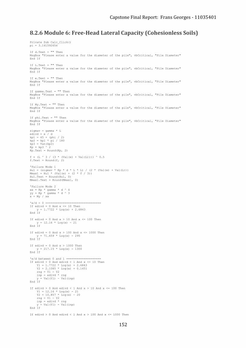
Capstone Final Report: Frans Georges - 11035401
152
8.2.6 Module 6: Free-Head Lateral Capacity (Cohesionless Soils)
Private Sub Calc_Click()
pi = 3.141592654
If d.Text = "" Then
MsgBox "Please enter a value for the diameter of the pile", vbCritical, "Pile Diameter"
End If
If L.Text = "" Then
MsgBox "Please enter a value for the diameter of the pile", vbCritical, "Pile Diameter"
End If
If e.Text = "" Then
MsgBox "Please enter a value for the diameter of the pile", vbCritical, "Pile Diameter"
End If
If gamma.Text = "" Then
MsgBox "Please enter a value for the diameter of the pile", vbCritical, "Pile Diameter"
End If
If My.Text = "" Then
MsgBox "Please enter a value for the diameter of the pile", vbCritical, "Pile Diameter"
End If
If phi.Text = "" Then
MsgBox "Please enter a value for the diameter of the pile", vbCritical, "Pile Diameter"
End If
sigmav = gamma * L
edivd = e / d
kp1 = 45 + (phi / 2)
kp2 = kp1 * pi / 180
kp3 = Tan(kp2)
Kp = kp3 ^ 2
Kp.Text = Round(Kp, 2)
f = (L ^ 3 / (3 * (Val(e) + Val(L)))) ^ 0.5
f.Text = Round(f, 2)
'Failure Mode 1
Hu1 = (sigmav * Kp * d * L * L) / (2 * (Val(e) + Val(L)))
Mmax1 = Hu1 * (Val(e) + (2 * f / 3))
Hu1.Text = Round(Hu1, 0)
Mmax1.Text = Round(Mmax1, 0)
'Failure Mode 2
xx = Kp * gamma * d ^ 4
yy = Kp * gamma * d ^ 3
x = My / xx
'e/d = 0 ================================
If edivd = 0 And x <= 10 Then
y = 1.7722 * Log(x) + 2.6843
End If
If edivd = 0 And x > 10 And x <= 100 Then
y = 12.16 * Log(x) - 21
End If
If edivd = 0 And x > 100 And x <= 1000 Then
y = 71.659 * Log(x) - 295
End If
If edivd = 0 And x > 1000 Then
y = 217.15 * Log(x) - 1300
End If
'e/d between 0 and 1 ====================
If edivd > 0 And edivd < 1 And x <= 10 Then
Y1 = 1.7722 * Log(x) + 2.6843
Y2 = 2.1085 * Log(x) + 0.1451
rng = Y1 - Y2
inp = edivd * rng
y = Val(Y1) - Val(inp)
End If
If edivd > 0 And edivd < 1 And x > 10 And x <= 100 Then
Y1 = 12.16 * Log(x) - 21
Y2 = 10.857 * Log(x) - 20
rng = Y1 - Y2
inp = edivd * rng
y = Val(Y1) - Val(inp)
End If
If edivd > 0 And edivd < 1 And x > 100 And x <= 1000 Then
Capstone Final Report: Frans Georges - 11035401
153
Y1 = 71.659 * Log(x) - 295
Y2 = 60.801 * Log(x) - 250
rng = Y1 - Y2
inp = edivd * rng
y = Val(Y1) - Val(inp)
End If
If edivd > 0 And edivd < 1 And x > 1000 Then
Y1 = 217.15 * Log(x) - 1300
Y2 = 219.32 * Log(x) - 1345
rng = Y1 - Y2
inp = edivd * rng
y = Val(Y1) - Val(inp)
End If
'e/d = 1 ================================
If edivd = 1 And x <= 10 Then
y = 2.1085 * Log(x) + 0.1451
End If
If edivd = 1 And x > 10 And x <= 100 Then
y = 10.857 * Log(x) - 20
End If
If edivd = 1 And x > 100 And x <= 1000 Then
y = 60.801 * Log(x) - 250
End If
If edivd = 1 And x > 1000 Then
y = 219.32 * Log(x) - 1345
End If
'e/d between 1 and 2 ====================
If edivd > 1 And edivd < 2 And x <= 10 Then
Y1 = 2.1085 * Log(x) + 0.1451
Y2 = 2.1641 * Log(x) - 0.9829
rng = Y1 - Y2
ed = Val(edivd) - 1
inp = ed * rng
y = Val(Y1) - Val(inp)
End If
If edivd > 1 And edivd < 2 And x > 10 And x <= 100 Then
Y1 = 10.857 * Log(x) - 20
Y2 = 9.1202 * Log(x) - 17
rng = Y1 - Y2
ed = Val(edivd) - 1
inp = ed * rng
y = Val(Y1) - Val(inp)
End If
If edivd > 1 And edivd < 2 And x > 100 And x <= 1000 Then
Y1 = 60.801 * Log(x) - 250
Y2 = 54.287 * Log(x) - 225
rng = Y1 - Y2
ed = Val(edivd) - 1
inp = ed * rng
y = Val(Y1) - Val(inp)
End If
If edivd > 1 And edivd < 2 And x > 1000 Then
Y1 = 219.32 * Log(x) - 1345
Y2 = 206.29 * Log(x) - 1275
rng = Y1 - Y2
ed = Val(edivd) - 1
inp = ed * rng
y = Val(Y1) - Val(inp)
End If
'e/d = 2 ================================
If edivd = 2 And x <= 10 Then
y = 2.1641 * Log(x) - 0.9829
End If
If edivd = 2 And x > 10 And x <= 100 Then
y = 9.1202 * Log(x) - 17
End If
If edivd = 2 And x > 100 And x <= 1000 Then
y = 54.287 * Log(x) - 225
End If
If edivd = 2 And x > 1000 Then
y = 206.29 * Log(x) - 1275
End If
'e/d between 2 and 4 ====================

Capstone Final Report: Frans Georges - 11035401
154
If edivd > 2 And edivd < 4 And x <= 10 Then
Y1 = 2.1641 * Log(x) - 0.9829
Y2 = 2.5047 * Log(x) - 2.7672
rng = Y1 - Y2
ed = (Val(edivd) - 2) / 2
inp = ed * rng
y = Val(Y1) - Val(inp)
End If
If edivd > 2 And edivd < 4 And x > 10 And x <= 100 Then
Y1 = 9.1202 * Log(x) - 17
Y2 = 7.383 * Log(x) - 14
rng = Y1 - Y2
ed = (Val(edivd) - 2) / 2
inp = ed * rng
y = Val(Y1) - Val(inp)
End If
If edivd > 2 And edivd < 4 And x > 100 And x <= 1000 Then
Y1 = 54.287 * Log(x) - 225
Y2 = 43.429 * Log(x) - 180
rng = Y1 - Y2
ed = (Val(edivd) - 2) / 2
inp = ed * rng
y = Val(Y1) - Val(inp)
End If
If edivd > 2 And edivd < 4 And x > 1000 Then
Y1 = 206.29 * Log(x) - 1275
Y2 = 197.6 * Log(x) - 1245
rng = Y1 - Y2
ed = (Val(edivd) - 2) / 2
inp = ed * rng
y = Val(Y1) - Val(inp)
End If
'e/d = 4 ================================
If edivd = 4 And x <= 10 Then
y = 2.5047 * Log(x) - 2.7672
End If
If edivd = 4 And x > 10 And x <= 100 Then
y = 7.383 * Log(x) - 14
End If
If edivd = 4 And x > 100 And x <= 1000 Then
y = 43.429 * Log(x) - 180
End If
If edivd = 4 And x > 1000 Then
y = 197.6 * Log(x) - 1245
End If
'e/d between 4 and 8 ====================
If edivd > 4 And edivd < 8 And x <= 10 Then
Y1 = 2.5047 * Log(x) - 2.7672
Y2 = 2.2407 * Log(x) - 3.6594
rng = Y1 - Y2
ed = (Val(edivd) - 4) / 4
inp = ed * rng
y = Val(Y1) - Val(inp)
End If
If edivd > 4 And edivd < 8 And x > 10 And x <= 100 Then
Y1 = 7.383 * Log(x) - 14
Y2 = 4.1258 * Log(x) - 8
rng = Y1 - Y2
ed = (Val(edivd) - 4) / 4
inp = ed * rng
y = Val(Y1) - Val(inp)
End If
If edivd > 4 And edivd < 8 And x > 100 And x <= 1000 Then
Y1 = 43.429 * Log(x) - 180
Y2 = 25.623 * Log(x) - 107
rng = Y1 - Y2
ed = (Val(edivd) - 4) / 4
inp = ed * rng
y = Val(Y1) - Val(inp)
End If
If edivd > 4 And edivd < 8 And x > 1000 Then
Y1 = 197.6 * Log(x) - 1245
Y2 = 186.75 * Log(x) - 1220
rng = Y1 - Y2
ed = (Val(edivd) - 4) / 4

Capstone Final Report: Frans Georges - 11035401
155
inp = ed * rng
y = Val(Y1) - Val(inp)
End If
'e/d = 8 ================================
If edivd = 8 And x <= 10 Then
y = 2.2407 * Log(x) - 3.6594
End If
If edivd = 8 And x > 10 And x <= 100 Then
y = 4.1258 * Log(x) - 8
End If
If edivd = 8 And x > 100 And x <= 1000 Then
y = 25.623 * Log(x) - 107
End If
If edivd = 8 And x > 1000 Then
y = 186.75 * Log(x) - 1220
End If
'e/d between 8 and 16 ===================
If edivd > 8 And edivd < 16 And x <= 10 Then
Y1 = 2.2407 * Log(x) - 3.6594
Y2 = 3.1067 * Log(x) - 8.3068
rng = Y1 - Y2
ed = (Val(edivd) - 8) / 8
inp = ed * rng
y = Val(Y1) - Val(inp)
End If
If edivd > 8 And edivd < 16 And x > 10 And x <= 100 Then
Y1 = 4.1258 * Log(x) - 8
Y2 = 3.1067 * Log(x) - 8.3068
rng = Y1 - Y2
ed = (Val(edivd) - 8) / 8
inp = ed * rng
y = Val(Y1) - Val(inp)
End If
If edivd > 8 And edivd < 16 And x > 100 And x <= 1000 Then
Y1 = 25.623 * Log(x) - 107
Y2 = 19.109 * Log(x) - 82
rng = Y1 - Y2
ed = (Val(edivd) - 8) / 8
inp = ed * rng
y = Val(Y1) - Val(inp)
End If
If edivd > 8 And edivd < 16 And x > 1000 Then
Y1 = 186.75 * Log(x) - 1220
Y2 = 152 * Log(x) - 1000
rng = Y1 - Y2
ed = (Val(edivd) - 8) / 8
inp = ed * rng
y = Val(Y1) - Val(inp)
End If
'e/d = 16 ===============================
If edivd = 16 And x <= 100 Then
y = 3.1067 * Log(x) - 8.3068
End If
If edivd = 16 And x > 100 And x <= 1000 Then
y = 19.109 * Log(x) - 82
End If
If edivd = 16 And x > 1000 Then
y = 152 * Log(x) - 1000
End If
'e/d between 16 and 32 ==================
If edivd > 16 And edivd < 32 And x <= 100 Then
Y1 = 3.1067 * Log(x) - 8.3068
Y2 = 1.9051 * Log(x) - 5.7732
rng = Y1 - Y2
ed = (Val(edivd) - 16) / 16
inp = ed * rng
y = Val(Y1) - Val(inp)
End If
If edivd > 16 And edivd < 32 And x > 100 And x <= 1000 Then
Y1 = 19.109 * Log(x) - 82
Y2 = 11.726 * Log(x) - 51
rng = Y1 - Y2
ed = (Val(edivd) - 16) / 16

Capstone Final Report: Frans Georges - 11035401
156
inp = ed * rng
y = Val(Y1) - Val(inp)
End If
If edivd > 16 And edivd < 32 And x > 1000 Then
Y1 = 152 * Log(x) - 1000
Y2 = 117.26 * Log(x) - 780
rng = Y1 - Y2
ed = (Val(edivd) - 16) / 16
inp = ed * rng
y = Val(Y1) - Val(inp)
End If
'e/d = 32 ===============================
If edivd = 32 And x <= 100 Then
y = 1.9051 * Log(x) - 5.7732
End If
If edivd = 32 And x > 100 And x <= 1000 Then
y = 11.726 * Log(x) - 51
End If
If edivd = 32 And x > 1000 Then
y = 117.26 * Log(x) - 780
End If
Hu2 = y * yy
Hu2.Text = Round(Hu2, 0)
Mmax2 = My
Mmax2.Text = Round(Mmax2, 0)
If Val(Hu1) < Val(Hu2) Then
FM = 1
End If
If Val(Hu2) < Val(Hu1) Then
FM = 2
End If
Label31.Visible = True
Label34.Visible = True
Label35.Visible = True
If FM = 1 Then
ResC = Round(Hu1, 0)
ResM = Round(Mmax1, 0)
ResFM.Caption = "Failure Mode 1"
ResHu.Caption = ResC & " kN"
ResMmax.Caption = ResM & " kNm"
fm1.Visible = True
fm2.Visible = False
End If
If FM = 2 Then
ResC = Round(Hu2, 0)
ResM = Round(Mmax2, 0)
ResFM.Caption = "Failure Mode 2"
ResHu.Caption = ResC & " kN"
ResMmax.Caption = ResM & " kNm"
fm1.Visible = False
fm2.Visible = True
End If
x.Text = Round(x, 0)
y.Text = Round(y, 0)
End Sub
Private Sub d_Change()
If IsNumeric(d.Text) Or d.Text = "" Then
Else: MsgBox "Please enter a numeric value", vbCritical, "Invalid Input"
d.Text = ""
End If
End Sub
Private Sub e_Change()
If IsNumeric(e.Text) Or e.Text = "" Then
Else: MsgBox "Please enter a numeric value", vbCritical, "Invalid Input"
e.Text = ""
End If
End Sub
Private Sub Exit_Click()
End
End Sub
Private Sub Form_Load()
fm1.Visible = False
fm2.Visible = False

Capstone Final Report: Frans Georges - 11035401
157
d.Text = ""
L.Text = ""
e.Text = ""
gamma.Text = ""
My.Text = ""
phi.Text = ""
sigmav.Text = ""
edivd.Text = ""
Kp.Text = ""
Hu1.Text = ""
Hu2.Text = ""
Mmax1.Text = ""
Mmax2.Text = ""
Label31.Visible = False
Label34.Visible = False
Label35.Visible = False
ResFM.Caption = ""
ResHu.Caption = ""
ResMmax.Caption = ""
x.Text = ""
y.Text = ""
End Sub
Private Sub gamma_Change()
If IsNumeric(gamma.Text) Or gamma.Text = "" Then
Else: MsgBox "Please enter a numeric value", vbCritical, "Invalid Input"
gamma.Text = ""
End If
End Sub
Private Sub L_Change()
If IsNumeric(L.Text) Or L.Text = "" Then
Else: MsgBox "Please enter a numeric value", vbCritical, "Invalid Input"
L.Text = ""
End If
End Sub
Private Sub Menu_Click()
Title.Show
Title.Top = (Screen.Height - Title.Height) / 2
Title.Left = (Screen.Width - Title.Width) / 2
Unload Me
End Sub
Private Sub My_Change()
If IsNumeric(My.Text) Or My.Text = "" Then
Else: MsgBox "Please enter a numeric value", vbCritical, "Invalid Input"
My.Text = ""
End If
End Sub
Private Sub phi_Change()
If IsNumeric(phi.Text) Or phi.Text = "" Then
Else: MsgBox "Please enter a numeric value", vbCritical, "Invalid Input"
phi.Text = ""
End If
End Sub
Private Sub Reset_Click()
Call Form_Load
End Sub

Capstone Final Report: Frans Georges - 11035401
158
8.2.7 Module 7: Fixed-Head Lateral Capacity (Cohesionless Soils) Private Sub Calc_Click()
pi = 3.141592654
sigmav = gamma * L
kp1 = 45 + (phi / 2)
kp2 = kp1 * pi / 180
kp3 = Tan(kp2)
Kp = kp3 ^ 2
Kp.Text = Round(Kp, 2)
' Failure Mode 1
Hu1 = 1.5 * sigmav * d * L * Kp
Hu1.Text = Round(Hu1, 0)
Mmax1 = (2 * Hu1 * L) / 3
Mmax1.Text = Round(Mmax1, 0)
'Failure Mode 2
Hu2 = ((0.5 * sigmav * d * L * L * Kp) + Val(My)) / L
Hu2.Text = Round(Hu2, 0)
f = ((2 * Hu2) / (3 * gamma * d * Kp)) ^ 0.5
f.Text = Round(f, 2)
Mmax2 = ((2 * Hu2 * f) / 3) - Val(My)
Mmax2.Text = Round(Mmax2, 0)
'Failure Mode 3
xx = Kp * gamma * d ^ 4
yy = Kp * gamma * d ^ 3
x = My / xx
x.Text = Round(x, 0)
If x <= 1 Then
y = 1.2459 * Log(x) + 2.5
End If
If x > 1 And x <= 10 Then
y = 4.5601 * Log(x) + 2.5
End If
If x > 10 And x <= 100 Then
y = 18.24 * Log(x) - 29
End If
If x > 100 And x <= 1000 Then
y = 84.687 * Log(x) - 335
End If
If x > 1000 Then
y = 325.72 * Log(x) - 2000
End If
y.Text = Round(y, 0)
Hu3 = y * yy
Hu3.Text = Round(Hu3, 0)
Mmax3 = My
Mmax3.Text = Round(Mmax3, 0)
'Determining Failure Mode
If Val(Hu1) < Val(Hu2) And Val(Hu1) < Val(Hu3) Then
FM = 1
End If
If Val(Hu2) < Val(Hu1) And Val(Hu2) < Val(Hu3) Then
FM = 2
End If
If Val(Hu3) < Val(Hu1) And Val(Hu3) < Val(Hu2) Then
FM = 3
End If
'Displaying results
Label33.Visible = True
Label34.Visible = True
Label35.Visible = True
If FM = 1 Then
ResC = Round(Hu1, 0)
ResM = Round(Mmax1, 0)
ResFM.Caption = "Failure Mode 1"
ResHu.Caption = ResC & " kN"
ResMmax.Caption = ResM & " kNm"
fm1.Visible = True
fm2.Visible = False
fm3.Visible = False
End If

Capstone Final Report: Frans Georges - 11035401
159
If FM = 2 Then
ResC = Round(Hu2, 0)
ResM = Round(Mmax2, 0)
ResFM.Caption = "Failure Mode 2"
ResHu.Caption = ResC & " kN"
ResMmax.Caption = ResM & " kNm"
fm1.Visible = False
fm2.Visible = True
fm3.Visible = False
End If
If FM = 3 Then
ResC = Round(Hu3, 0)
ResM = Round(Mmax3, 0)
ResFM.Caption = "Failure Mode 3"
ResHu.Caption = ResC & " kN"
ResMmax.Caption = ResM & " kNm"
fm1.Visible = False
fm2.Visible = False
fm3.Visible = True
End If
End Sub
Private Sub d_Change()
If IsNumeric(d.Text) Or d.Text = "" Then
Else: MsgBox "Please enter a numeric value", vbCritical, "Invalid Input"
d.Text = ""
End If
End Sub
Private Sub Exit_Click()
End
End Sub
Private Sub Form_Load()
fm1.Visible = False
fm2.Visible = False
fm3.Visible = False
d.Text = ""
L.Text = ""
gamma.Text = ""
My.Text = ""
phi.Text = ""
sigmav.Text = ""
f.Text = ""
Kp.Text = ""
Hu1.Text = ""
Hu2.Text = ""
Hu3.Text = ""
Mmax1.Text = ""
Mmax2.Text = ""
Mmax3.Text = ""
Label33.Visible = False
Label34.Visible = False
Label35.Visible = False
ResFM.Caption = ""
ResHu.Caption = ""
ResMmax.Caption = ""
x.Text = ""
y.Text = ""
End Sub
Private Sub gamma_Change()
If IsNumeric(gamma.Text) Or gamma.Text = "" Then
Else: MsgBox "Please enter a numeric value", vbCritical, "Invalid Input"
gamma.Text = ""
End If
End Sub
Private Sub L_Change()
If IsNumeric(L.Text) Or L.Text = "" Then
Else: MsgBox "Please enter a numeric value", vbCritical, "Invalid Input"
L.Text = ""
End If
End Sub
Private Sub Menu_Click()
Title.Show
Title.Top = (Screen.Height - Title.Height) / 2
Title.Left = (Screen.Width - Title.Width) / 2
Unload Me
End Sub
Private Sub My_Change()
If IsNumeric(My.Text) Or My.Text = "" Then
Else: MsgBox "Please enter a numeric value", vbCritical, "Invalid Input"

Capstone Final Report: Frans Georges - 11035401
160
My.Text = ""
End If
End Sub
Private Sub phi_Change()
If IsNumeric(phi.Text) Or phi.Text = "" Then
Else: MsgBox "Please enter a numeric value", vbCritical, "Invalid Input"
phi.Text = ""
End If
End Sub
Private Sub Reset_Click()
Call Form_Load
End Sub

Capstone Final Report: Frans Georges - 11035401
161
8.2.8 Module 8: Vertical Settlement of a Single Floating Pile
Private Sub Calc_Click()
pi = 3.141592654
Ldivd = L / dout 'L/d ratio
If Ldivd < 1 Then Ldivd = 1 'use a minimum value of 1 for L/d
Ldivd.Text = Round(Ldivd, 2)
rout = dout / 2 'outer radius
rin = din / 2 'inner radius
Ag = pi * rout * rout 'gross area
Ain = pi * rin * rin 'hollow area
Asec = Val(Ag) - Val(Ain) 'cross-sectional area
Ra = Asec / Ag 'Determine R_A value
Ra.Text = Round(Ra, 2) 'Round R_A to 2 decimal places
K = (Ep / Es) * Ra 'Determine K value
K.Text = Round(K, 2) 'Round K to 2 decimal places
'L/d = 1 ================================
If Ldivd = 1 And K <= 100 Then
Ip = -0.0565 * Log(K) + 0.66
End If
If Ldivd = 1 And K > 100 And K <= 1000 Then
Ip = -0.0217 * Log(K) + 0.5
End If
If Ldivd = 1 And K > 1000 Then
Ip = 0.35
End If
'L/d between 1 and 2 ====================
If Ldivd > 1 And Ldivd < 2 And K <= 100 Then
I1 = -0.0565 * Log(K) + 0.66
I2 = -0.0738 * Log(K) + 1.07
rng = I2 - I1
Ld = Val(Ldivd) - 1
inp = Ld * rng
Ip = Val(I1) + Val(inp)
End If
If Ldivd > 1 And Ldivd < 2 And K > 100 And K <= 1000 Then
I1 = -0.0217 * Log(K) + 0.5
I2 = -0.013 * Log(K) + 0.79
rng = I2 - I1
Ld = Val(Ldivd) - 1
inp = Ld * rng
Ip = Val(I1) + Val(inp)
End If
If Ldivd > 1 And Ldivd < 2 And K > 1000 Then
I1 = 0.35
I2 = 0.7
rng = I2 - I1
Ld = Val(Ldivd) - 1
inp = Ld * rng
Ip = Val(I1) + Val(inp)
End If
'L/d = 2 ================================
If Ldivd = 2 And K <= 100 Then
Ip = -0.0738 * Log(K) + 1.07
End If
If Ldivd = 2 And K > 100 And K <= 1000 Then
Ip = -0.013 * Log(K) + 0.79
End If
If Ldivd = 2 And K > 1000 Then
Ip = 0.7
End If
'L/d between 2 and 5 ====================
If Ldivd > 2 And Ldivd < 5 And K <= 100 Then
I1 = -0.0738 * Log(K) + 1.07
I2 = -0.2606 * Log(K) + 2.5
rng = I2 - I1
Ld = (Val(Ldivd) - 2) / 3
inp = Ld * rng
Ip = Val(I1) + Val(inp)
End If
If Ldivd > 2 And Ldivd < 5 And K > 100 And K <= 1000 Then
I1 = -0.013 * Log(K) + 0.79

Capstone Final Report: Frans Georges - 11035401
162
I2 = -0.0869 * Log(K) + 1.7
rng = I2 - I1
Ld = (Val(Ldivd) - 2) / 3
inp = Ld * rng
Ip = Val(I1) + Val(inp)
End If
If Ldivd > 2 And Ldivd < 5 And K > 1000 Then
I1 = 0.7
I2 = 1.1
rng = I2 - I1
Ld = (Val(Ldivd) - 2) / 3
inp = Ld * rng
Ip = Val(I1) + Val(inp)
End If
'L/d = 5 ================================
If Ldivd = 5 And K <= 100 Then
Ip = -0.2606 * Log(K) + 2.5
End If
If Ldivd = 5 And K > 100 And K <= 1000 Then
Ip = -0.0869 * Log(K) + 1.7
End If
If Ldivd = 5 And K > 1000 Then
Ip = 1.1
End If
'L/d between 5 and 10 ===================
If Ldivd > 5 And Ldivd < 10 And K <= 100 Then
I1 = -0.2606 * Log(K) + 2.5
I2 = -0.7383 * Log(K) + 5.3
rng = I2 - I1
Ld = (Val(Ldivd) - 5) / 5
inp = Ld * rng
Ip = Val(I1) + Val(inp)
End If
If Ldivd > 5 And Ldivd < 10 And K > 100 And K <= 1000 Then
I1 = -0.0869 * Log(K) + 1.7
I2 = -0.1954 * Log(K) + 2.8
rng = I2 - I1
Ld = (Val(Ldivd) - 5) / 5
inp = Ld * rng
Ip = Val(I1) + Val(inp)
End If
If Ldivd > 5 And Ldivd < 10 And K > 1000 Then
I1 = 1.1
I2 = -0.0217 * Log(K) + 1.6
rng = I2 - I1
Ld = (Val(Ldivd) - 5) / 5
inp = Ld * rng
Ip = Val(I1) + Val(inp)
End If
'L/d = 10 ===============================
If Ldivd = 10 And K <= 100 Then
Ip = -0.7383 * Log(K) + 5.3
End If
If Ldivd = 10 And K > 100 And K <= 1000 Then
Ip = -0.1954 * Log(K) + 2.8
End If
If Ldivd = 10 And K > 1000 Then
Ip = -0.0217 * Log(K) + 1.6
End If
'L/d between 10 and 25 ==================
If Ldivd > 10 And Ldivd < 25 And K <= 100 Then
I1 = -0.7383 * Log(K) + 5.3
I2 = -1.7372 * Log(K) + 11.7
rng = I2 - I1
Ld = (Val(Ldivd) - 10) / 15
inp = Ld * rng
Ip = Val(I1) + Val(inp)
End If
If Ldivd > 10 And Ldivd < 25 And K > 100 And K <= 1000 Then
I1 = -0.1954 * Log(K) + 2.8
I2 = -0.6514 * Log(K) + 6.7
rng = I2 - I1
Ld = (Val(Ldivd) - 10) / 15
inp = Ld * rng
Ip = Val(I1) + Val(inp)
End If

Capstone Final Report: Frans Georges - 11035401
163
If Ldivd > 10 And Ldivd < 25 And K > 1000 Then
I1 = -0.0217 * Log(K) + 1.6
I2 = -0.152 * Log(K) + 3.25
rng = I2 - I1
Ld = (Val(Ldivd) - 10) / 15
inp = Ld * rng
Ip = Val(I1) + Val(inp)
End If
'L/d = 25 ===============================
If Ldivd = 25 And K <= 100 Then
Ip = -1.7372 * Log(K) + 11.7
End If
If Ldivd = 25 And K > 100 And K <= 1000 Then
Ip = -0.6514 * Log(K) + 6.7
End If
If Ldivd = 25 And K > 1000 Then
Ip = -0.152 * Log(K) + 3.25
End If
'L/d between 25 and 50 ==================
If Ldivd > 25 And Ldivd < 50 And K <= 100 Then
I1 = -1.7372 * Log(K) + 11.7
I2 = -2.6926 * Log(K) + 19.2
rng = I2 - I1
Ld = (Val(Ldivd) - 25) / 25
inp = Ld * rng
Ip = Val(I1) + Val(inp)
End If
If Ldivd > 25 And Ldivd < 50 And K > 100 And K <= 1000 Then
I1 = -0.6514 * Log(K) + 6.7
I2 = -1.5635 * Log(K) + 14
rng = I2 - I1
Ld = (Val(Ldivd) - 25) / 25
inp = Ld * rng
Ip = Val(I1) + Val(inp)
End If
If Ldivd > 25 And Ldivd < 50 And K > 1000 Then
I1 = -0.152 * Log(K) + 3.25
I2 = -0.3909 * Log(K) + 5.9
rng = I2 - I1
Ld = (Val(Ldivd) - 25) / 25
inp = Ld * rng
Ip = Val(I1) + Val(inp)
End If
'L/d = 50 ===============================
If Ldivd = 50 And K <= 100 Then
Ip = -2.6926 * Log(K) + 19.2
End If
If Ldivd = 50 And K > 100 And K <= 1000 Then
Ip = -1.5635 * Log(K) + 14
End If
If Ldivd = 50 And K > 1000 Then
Ip = -0.3909 * Log(K) + 5.9
End If
'L/d between 50 and 100 =================
If Ldivd > 50 And Ldivd < 100 And K <= 100 Then
I1 = -2.6926 * Log(K) + 19.2
I2 = -3.9087 * Log(K) + 30
rng = I2 - I1
Ld = (Val(Ldivd) - 50) / 50
inp = Ld * rng
Ip = Val(I1) + Val(inp)
End If
If Ldivd > 50 And Ldivd < 100 And K > 100 And K <= 1000 Then
I1 = -1.5635 * Log(K) + 14
I2 = -2.9966 * Log(K) + 25.8
rng = I2 - I1
Ld = (Val(Ldivd) - 50) / 50
inp = Ld * rng
Ip = Val(I1) + Val(inp)
End If
If Ldivd > 50 And Ldivd < 100 And K > 1000 Then
I1 = -0.3909 * Log(K) + 5.9
I2 = -0.912 * Log(K) + 11.4
rng = I2 - I1
Ld = (Val(Ldivd) - 50) / 50

Capstone Final Report: Frans Georges - 11035401
164
inp = Ld * rng
Ip = Val(I1) + Val(inp)
End If
'L/d = 100 ==============================
If Ldivd = 100 And K <= 100 Then
Ip = -3.9087 * Log(K) + 30
End If
If Ldivd = 100 And K > 100 And K <= 1000 Then
Ip = -2.9966 * Log(K) + 25.8
End If
If Ldivd = 100 And K > 1000 Then
Ip = -0.912 * Log(K) + 11.4
End If
'L/d between 100 and 200 ================
If Ldivd > 100 And Ldivd < 200 And K <= 100 Then
I1 = -3.9087 * Log(K) + 30
I2 = -4.3429 * Log(K) + 38
rng = I2 - I1
Ld = (Val(Ldivd) - 100) / 100
inp = Ld * rng
Ip = Val(I1) + Val(inp)
End If
If Ldivd > 100 And Ldivd < 200 And K > 100 And K <= 1000 Then
I1 = -2.9966 * Log(K) + 25.8
I2 = -3.6915 * Log(K) + 35
rng = I2 - I1
Ld = (Val(Ldivd) - 100) / 100
inp = Ld * rng
Ip = Val(I1) + Val(inp)
End If
If Ldivd > 100 And Ldivd < 200 And K > 1000 Then
I1 = -0.912 * Log(K) + 11.4
I2 = -2.2583 * Log(K) + 25.1
rng = I2 - I1
Ld = (Val(Ldivd) - 100) / 100
inp = Ld * rng
Ip = Val(I1) + Val(inp)
End If
'L/d = 200 ==============================
If Ldivd = 200 And K <= 100 Then
Ip = -4.3429 * Log(K) + 38
End If
If Ldivd = 200 And K > 100 And K <= 1000 Then
Ip = -3.6915 * Log(K) + 35
End If
If Ldivd = 200 And K > 1000 Then
Ip = -2.2583 * Log(K) + 25.1
End If
Label18.Visible = True 'Show label stating The settlement of the pile is...
Ip.Text = Round(Ip, 2) 'Round I value to 2 decimal places
S = ((P / (L * Es)) * Ip) 'Calculate S value in mm
S = Round(S, 1) 'Round S value to whole number
S.Caption = Val(S) & " mm" 'Output settlement
End Sub
Private Sub din_Change()
If IsNumeric(din.Text) Or din.Text = "" Then
Else: MsgBox "Please enter a numeric value", vbCritical, "Invalid Input"
din.Text = ""
End If
End Sub
Private Sub dout_Change()
If IsNumeric(dout.Text) Or dout.Text = "" Then
Else: MsgBox "Please enter a numeric value", vbCritical, "Invalid Input"
dout.Text = ""
End If
End Sub
Private Sub Ep_Change()
If IsNumeric(Ep.Text) Or Ep.Text = "" Then
Else: MsgBox "Please enter a numeric value", vbCritical, "Invalid Input"
Ep.Text = ""
End If
End Sub
Private Sub Es_Change()

Capstone Final Report: Frans Georges - 11035401
165
If IsNumeric(Es.Text) Or Es.Text = "" Then
Else: MsgBox "Please enter a numeric value", vbCritical, "Invalid Input"
Es.Text = ""
End If
End Sub
Private Sub Exit_Click()
End
End Sub
Private Sub Form_Load()
P.Text = ""
L.Text = ""
dout.Text = ""
din.Text = ""
Es.Text = ""
Ep.Text = ""
Ldivd.Text = ""
K.Text = ""
Ra.Text = ""
Ip.Text = ""
S.Caption = ""
Label18.Visible = False
End Sub
Private Sub L_Change()
If IsNumeric(L.Text) Or L.Text = "" Then
Else: MsgBox "Please enter a numeric value", vbCritical, "Invalid Input"
L.Text = ""
End If
End Sub
Private Sub Menu_Click()
Title.Show
Title.Top = (Screen.Height - Title.Height) / 2
Title.Left = (Screen.Width - Title.Width) / 2
Unload Me
End Sub
Private Sub P_Change()
If IsNumeric(P.Text) Or P.Text = "" Then
Else: MsgBox "Please enter a numeric value", vbCritical, "Invalid Input"
P.Text = ""
End If
End Sub
Private Sub Reset_Click()
Call Form_Load
End Sub