Final exam practice solutionsJoshua Loftus

Question 1

We will fit a linear model using the diamonds dataset. There are two continuous variables, price and carat(the weight of the diamond), and three categorical variables (cut, color, clarity). The first few rows ofdata are shown below.

## # A tibble: 6 x 5## carat cut color clarity price## <dbl> <fct> <fct> <fct> <int>## 1 0.230 Premium Good Bad 326## 2 0.210 Premium Good Bad 326## 3 0.230 OK Good Good 327## 4 0.290 Premium Bad Good 334## 5 0.310 OK Bad Bad 335## 6 0.240 OK Bad Good 336

There are 53940 rows in this dataset, each one is an observation corresponding to an individual diamond.Before analyzing the data, we first split it into two random subsets, a training set with 5394 observationsand a test set with 29976 observations.

Part (a)

#### Call:## lm(formula = log(price) ~ carat + cut, data = dtrain)#### Residuals:## Min 1Q Median 3Q Max## -5.1155 -0.2558 0.0371 0.2612 1.4082#### Coefficients:## Estimate Std. Error t value Pr(>|t|)## (Intercept) 6.20247 0.01350 459.585 < 2e-16 ***## carat 1.94227 0.01146 169.440 < 2e-16 ***## cutPremium 0.04834 0.01161 4.164 3.18e-05 ***## ---## Signif. codes: 0 '***' 0.001 '**' 0.01 '*' 0.05 '.' 0.1 ' ' 1#### Residual standard error: 0.4035 on 5391 degrees of freedom## Multiple R-squared: 0.842, Adjusted R-squared: 0.842## F-statistic: 1.437e+04 on 2 and 5391 DF, p-value: < 2.2e-16

• What outcome variable is this model predicting?

Solution:

The outcome is log(price), the logarithm of the selling price of each diamond

1

• What are the predictor variables?

Solution:

The predictors are carat (weight) and cut

• What is the interpretation of the coefficient for carat? Does the fact that this coefficient is positivesurprise you, or is it what you would expect?

Solution:

The coefficient value, about 1.97, is the increase in the predicted log(price) for each increase of one unitin the carat predictor while holding cut constant. The positive value is expected since larger diamondsgenerally cost more.

• What are the interpretations for the coefficients of (Intercept) and cutPremium? Which one is larger,and does that surprise you or is it expected?

Solution:

The intercept coefficient, about 6.19, is the predicted value for a weightless diamond with an OK value forcut, and the cutPremium coefficient, about 0.04, is the shift in this intercept for diamonds with Premiumvalue for the cut categorical predictor.

The fact that cutPremium has a positive coefficient means that the intercept for Premium diamonds is largerthan the overall intercept, which is expected.

• Why are all the p-values extremely small even though the coefficients are not very large?

Solution:

The sample size is large, about 5,000. Since the sample is so large, statisticial significance might not implypractical significance.

• What is the null hypothesis for the p-value in the first row of the summary (the row for the caratvariable)?

Solution:

The null is that the coefficient for carat in this model is zero. We could write this as H0 : βcarat = 0. Itmeans that there is no predicted change in the outcome due to the carat variable when holding cut constant.

• What is the null hypothesis for the p-value in the last line of the summary (the line with an F-statistic)?

Solution:

The default F -test shown at the bottom of the summary() compares the intercept only model to the fullmodel. So the null hypothesis is that the intercept only model is good enough when compared to the modelwith carat and cut.

• How would you interpret the adjusted R-squared for this model?

Solution:

2

The adjusted R-squared value of about 0.84 means that approximately 84% of the variation in log(price)can be explained using this linear model with carat and cut, and about 16% of the variation is unexplainedby the model.

Part (b)

498

44485379

−4

−2

0

8 10 12 14

Fitted values

Res

idua

ls

Residuals vs Fitted

498

44485379

−10

−5

0

−4 −2 0 2 4

Theoretical QuantilesS

tand

ardi

zed

resi

dual

s

Normal Q−Q

498

44485379

0

1

2

3

8 10 12 14

Fitted values

Sta

ndar

dize

d re

sidu

als

Scale−Location

498

44485379

−10

−5

0

OK Premium

Factor Level Combination

Sta

ndar

dize

d R

esid

uals

Contanst Leverage:Residuals vs Factor Levels

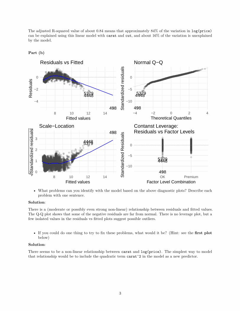
• What problems can you identify with the model based on the above diagnostic plots? Describe eachproblem with one sentence.

Solution:

There is a (moderate or possibly even strong non-linear) relationship between residuals and fitted values.The Q-Q plot shows that some of the negative residuals are far from normal. There is no leverage plot, but afew isolated values in the residuals vs fitted plots suggest possible outliers.

• If you could do one thing to try to fix these problems, what would it be? (Hint: see the first plotbelow)

Solution:

There seems to be a non-linear relationship between carat and log(price). The simplest way to modelthat relationship would be to include the quadratic term caratˆ2 in the model as a new predictor.

3

1e+04

1e+06

0 1 2 3 4

carat

pric

e

cut

OK

Premium

5

6

7

8

9

10

0 1 2 3 4

carat

log(

pric

e)

cut

OK

Premium

color

Good

Bad

4

Part (c)

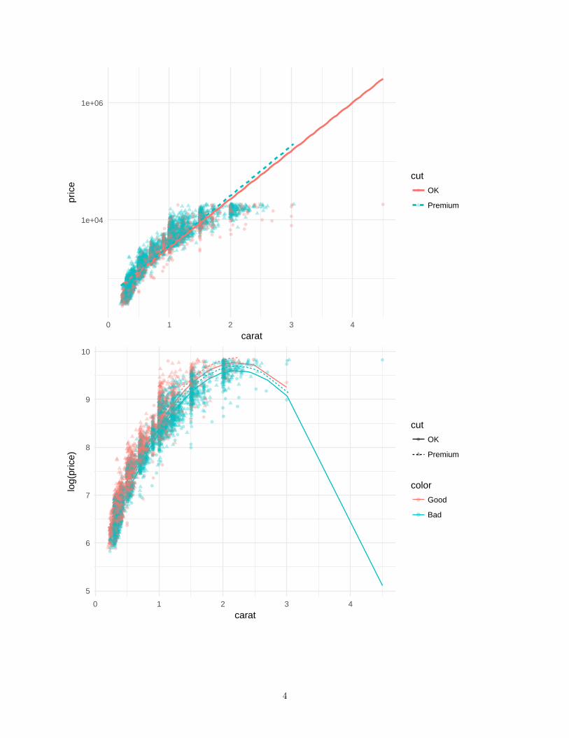
• The second plot above shows four lines which are predictions given by a new model, Model 2. Whatpredictor variables are in this new model? (Hint: there are more than one new variables included)

Solution:

The non-linear relationship between predicted values and carat suggests that the model has caratˆ2 as apredictor. The legend of the plot showing a new categorical variable, color, suggests that this variable hasalso been included as a predictor. So the new model is log(price) ~ carat + caratˆ2 + cut + color

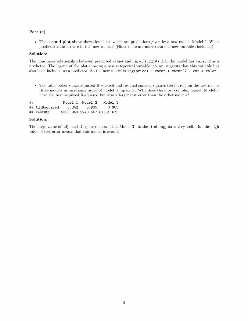
• The table below shows adjusted R-squared and residual sums of squares (test error) on the test set forthree models in increasing order of model complexity. Why does the most complex model, Model 3,have the best adjusted R-squared but also a larger test error than the other models?

## Model 1 Model 2 Model 3## AdjRsquared 0.842 0.935 0.965## TestRSS 5386.943 2248.667 67031.673

Solution:

The large value of adjusted R-squared shows that Model 3 fits the (training) data very well. But the highvalue of test error means that this model is overfit.

5

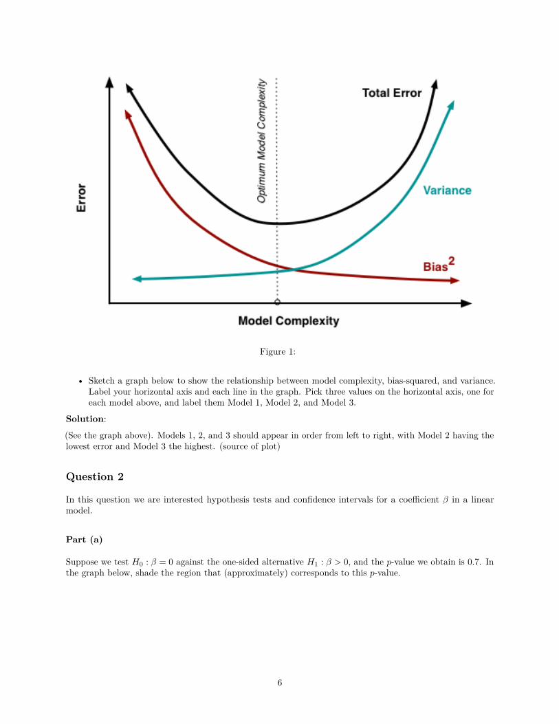
Figure 1:

• Sketch a graph below to show the relationship between model complexity, bias-squared, and variance.Label your horizontal axis and each line in the graph. Pick three values on the horizontal axis, one foreach model above, and label them Model 1, Model 2, and Model 3.

Solution:

(See the graph above). Models 1, 2, and 3 should appear in order from left to right, with Model 2 having thelowest error and Model 3 the highest. (source of plot)

Question 2

In this question we are interested hypothesis tests and confidence intervals for a coefficient β in a linearmodel.

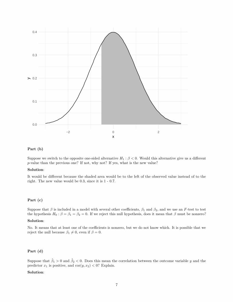
Part (a)

Suppose we test H0 : β = 0 against the one-sided alternative H1 : β > 0, and the p-value we obtain is 0.7. Inthe graph below, shade the region that (approximately) corresponds to this p-value.

6

0.0

0.1

0.2

0.3

0.4

−2 0 2

x

y

Part (b)

Suppose we switch to the opposite one-sided alternative H1 : β < 0. Would this alternative give us a differentp-value than the previous one? If not, why not? If yes, what is the new value?

Solution:

It would be different because the shaded area would be to the left of the observed value instead of to theright. The new value would be 0.3, since it is 1 - 0.7.

Part (c)

Suppose that β is included in a model with several other coefficients, β1 and β2, and we use an F -test to testthe hypothesis H0 : β = β1 = β2 = 0. If we reject this null hypothesis, does it mean that β must be nonzero?

Solution:

No. It means that at least one of the coefficients is nonzero, but we do not know which. It is possible that wereject the null because β1 6= 0, even if β = 0.

Part (d)

Suppose that β̂1 > 0 and β̂2 < 0. Does this mean the correlation between the outcome variable y and thepredictor x1 is positive, and cor(y, x2) < 0? Explain.

Solution:

7

No. The regression coefficient and correlation have the same sign if we are doing a simple regression withonly one predictor variable, but in a multiple regression it is possible for the coefficient to have a differentsign than the correlation. Simpson’s paradox is an example where the direction of the relationship changesdepending on whether you hold another predictor constant (in the multiple regression model) or not (in thecorrelation).

Part (e)

Suppose observations in the dataset correspond to small geographic regions like neighborhoods, y is the rateof emergency room visits from that neighborhood due to asthma, and x1 measures the concentration of airpollution. True or false, and explain: β1 is the increase in rate of ER visits due to asthma caused by pollution,holding other predictors constant.

Solution:

No, because association is not causation!

8