final project report jarrah and nitens report v10 - · pdf filethis report can also ... the...
TRANSCRIPT
`
Investigation of NDE technologies for drying quality segregation to aim for optimal kiln schedules to reduce drying degrade and accelerate kiln throughput in the hardwood sawmilling industry
PROJECT NUMBER: PNB126-0809 DECEMBER 2010
PROCESSING
This report can also be viewed on the FWPA website
www.fwpa.com.auFWPA Level 4, 10-16 Queen Street,
Melbourne VIC 3000, AustraliaT +61 (0)3 9927 3200 F +61 (0)3 9927 3288
E [email protected] W www.fwpa.com.au

Investigation of NDE technologies for drying quality
segregation to aim for optimal kiln schedules to reduce drying degrade and accelerate kiln
throughput in the hardwood sawmilling industry
Prepared for
Forest & Wood Products Australia
by
Roger Meder, Jun Li Yang, Philip Blakemore, Andrew Morrow, Dung Ngo, Nick Ebdon, Matthew Josh, Muruga Muruganathan

Forest & Wood Products Australia Limited Level 4, 10-16 Queen St, Melbourne, Victoria, 3000 T +61 3 9927 3200 F +61 3 9927 3288 E [email protected] W www.fwpa.com.au
Publication: Investigation of NDE technologies for drying qualit y segregation to aim for optimal kiln schedules to reduce drying degrade and accelerate kiln throughput in the hardwood sawmilling industry
Project No: PNB126-0809 © 2009 Forest & Wood Products Australia Limited. All rights reserved. Forest & Wood Products Australia Limited (FWPA) makes no warranties or assurances with respect to this publication including merchantability, fitness for purpose or otherwise. FWPA and all persons associated with it exclude all liability (including liability for negligence) in relation to any opinion, advice or information contained in this publication or for any consequences arising from the use of such opinion, advice or information. This work is copyright and protected under the Copyright Act 1968 (Cth). All material except the FWPA logo may be reproduced in whole or in part, provided that it is not sold or used for commercial benefit and its source (Forest & Wood Products Australia Limited) is acknowledged. Reproduction or copying for other purposes, which is strictly reserved only for the owner or licensee of copyright under the Copyright Act, is prohibited without the prior written consent of Forest & Wood Products Australia Limited. ISBN: 978-1-921763-35-9 Researcher/s: Roger Meder CSIRO Plant Industry, QLD Bioscience Precinct, 306 Carmody Rd, St Lucia 4067, Australia Jun Li Yang PO Box 4399, Melbourne University, Vic 3052 Philip Blakemore Andrew Morrow Dung Ngo CSIRO Materials Science and Engineering, Graham Rd, Highett, Vic 3190, Australia Nick Ebdon CSIRO Plant Industry, c/- CSIRO (CMSE), Private Bag 10, Clayton South, Vic 3169, Australia Matthew Josh CSIRO Earth Science and Resource Engineering Australian Resources Research Centre, PO Box 1130, Bentley WA 6102, Australia Muruga Muruganathan Retired Final report received by FWPA in December, 2010
i
Executive Summary Objectives The objectives of this study were:
1. Assess drying degrade in terms of check and collapse development
2. Identify whether simple wood properties of density or extractives content affect
the lumber relative drying rate of jarrah and shinning gum, and
3. Trial two technologies (acoustics and NIR) to test their ability to segregate green
lumber prior to drying in order to segregate individual boards into “fast” or “slow”
drying batches.
Key Results The major results of this study were:
Drying rate decreased with the increase of most of extractive contents in both
species.
Drying rate decreased with the increase of green density in E. nitens, but it did not
vary much with green density in jarrah.
The primary predictor for the number of internal checks differed between species.
It was initial moisture content in jarrah, and was area collapse in E. nitens.
The primary predictor for the area of internal checks also differed between
species. It was collapse-free area shrinkage in jarrah, and was area collapse in E.
nitens.
No single wood property or acoustic and ultrasonic variable was closely
correlated with drying rate, the number and area of internal checks, or collapse.
This means that none of these properties alone had potential to reliably predict
drying rate and drying degrade.
No acoustic and ultrasonic velocities when combined (without wood property
variables in the regression) were significant in the prediction of drying degrade
and collapse for both species. The along-grain acoustic and ultrasonic velocity VLL
appeared to provide some level of prediction to drying rate of jarrah with moderate
R2.
ii
The adjusted multiple regression R2 (wood properties as predictor variables)
ranged from 0.19 to 0.80. Whilst high R2 values are encouraging, it may not be
feasible in practice to sort or identify wood materials (at log or board levels) for
drying rate and drying degrade by measuring these significant wood properties.
Some important predictor variables vary between the 12% MC and 17% MC
datasets in multiple regression results, probably at least partly due to high levels
of inter-correlation between predictor variables, which then might have changed
the prediction results.
Log height was a consistently “influencing” variable in E. nitens. Drying rate
increased, but drying degrade and collapse decreased, in upper logs. Log heights
also had some effect in jarrah. Both drying degrade and collapse increased in
upper jarrah logs.
Near infrared spectroscopy showed moderate correlations for several properties,
many of which can currently only measured be measured destructively and with
great difficulty. While individually these properties are of limited interest,
collectively they may be able to identify the worst performing boards in order to
segregate them for alternate processing (e.g. milder drying conditions).
The dielectric constant measured on boards was unable to predict any single
property of interest.
The apparent diffusion tensor as determined by diffusion tensor imaging does not
correlate with the drying constant, but does show an order of magnitude greater
diffusion in E. marginata than E. nitens.
iii
Table of Contents Executive Summary ...................................................................................................... i 1. Introduction ............................................................................................................. 1 2. Methodology ........................................................................................................... 4
2.1 Log selection and sawing .................................................................................. 4 2.2 Specimen preparation ....................................................................................... 8 2.3 Data Acquisition .............................................................................................. 10
2.3.1 Acoustic velocities of full-length boards and 400mm drying rate sample boards ............................................................................................................... 10 2.3.2 Near infra-red (NIR) spectroscopy ............................................................ 12 2.3.3 Ultrasonic velocities .................................................................................. 13 2.3.4 Acoustic tomograph .................................................................................. 16 2.3.5 Dielectric property measurements ............................................................ 17 2.3.6 Diffusion tensor imaging ........................................................................... 18 2.3.7 Moisture content and basic density .......................................................... 20 2.3.8 Extractive content measurements ............................................................ 21 2.3.9 Drying rate ................................................................................................ 23 2.3.10 Collapse, shrinkages and internal checks .............................................. 27 2.3.11 Shrinkage potential ................................................................................. 30 2.3.12 Shrinkage in 2mm collapse-free sections (green to oven-dry) ................ 31 2.3.13 Data Analysis.......................................................................................... 31
3. Results and Discussion ........................................................................................ 33 3.1. Assessment of drying rate and drying degrade .............................................. 33
3.1.1 Drying rate ................................................................................................ 33 3.1.2 Surface checking ...................................................................................... 34 3.1.3 Collapse and internal checking – jarrah .................................................... 35 3.1.4 Collapse and internal checking – E. nitens ............................................... 36
3.2 Relationships of wood properties to drying rate and drying degrade .............. 38 3.2.1 Simple relationships ................................................................................. 38 3.2.2 Prediction of drying rate and drying degrade (jarrah) ............................... 43 3.2.2 Prediction of drying rate and drying degrade (E. nitens) ........................... 48
3.3 Potential of NDE technologies in board segregation for drying rate and drying degrade ................................................................................................................. 52
3.3.1 NIR ........................................................................................................... 52 3.3.2 Acoustic and ultrasonic velocities ............................................................. 56 3.3.3 Acoustic tomography ................................................................................ 60 3.3.4 Dielectric constants .................................................................................. 62 3.3.4 Diffusion tensor imaging ....................................................................... 62
4. Conclusions .......................................................................................................... 66 5. Recommendations ................................................................................................ 68 6. References ........................................................................................................... 68 7. Acknowledgements .............................................................................................. 70 8. Appendices ........................................................................................................... 71
1
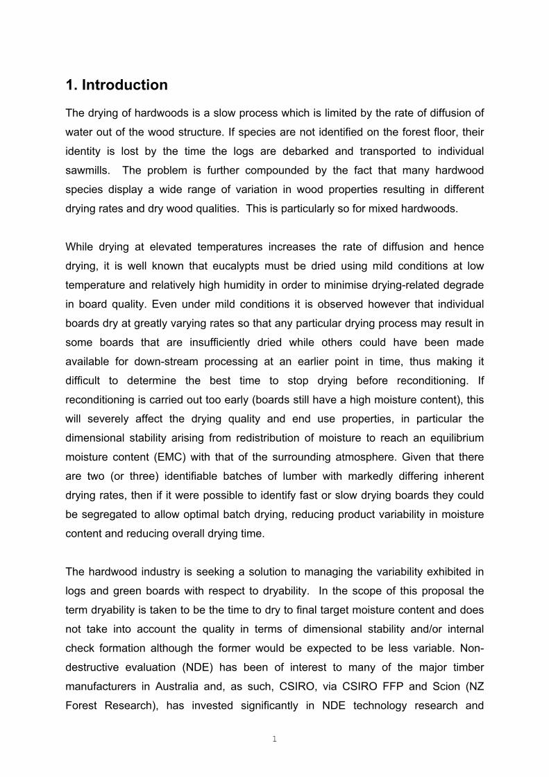
1. Introduction The drying of hardwoods is a slow process which is limited by the rate of diffusion of
water out of the wood structure. If species are not identified on the forest floor, their
identity is lost by the time the logs are debarked and transported to individual
sawmills. The problem is further compounded by the fact that many hardwood
species display a wide range of variation in wood properties resulting in different
drying rates and dry wood qualities. This is particularly so for mixed hardwoods.
While drying at elevated temperatures increases the rate of diffusion and hence
drying, it is well known that eucalypts must be dried using mild conditions at low
temperature and relatively high humidity in order to minimise drying-related degrade
in board quality. Even under mild conditions it is observed however that individual
boards dry at greatly varying rates so that any particular drying process may result in
some boards that are insufficiently dried while others could have been made
available for down-stream processing at an earlier point in time, thus making it
difficult to determine the best time to stop drying before reconditioning. If
reconditioning is carried out too early (boards still have a high moisture content), this
will severely affect the drying quality and end use properties, in particular the
dimensional stability arising from redistribution of moisture to reach an equilibrium
moisture content (EMC) with that of the surrounding atmosphere. Given that there
are two (or three) identifiable batches of lumber with markedly differing inherent
drying rates, then if it were possible to identify fast or slow drying boards they could
be segregated to allow optimal batch drying, reducing product variability in moisture
content and reducing overall drying time.
The hardwood industry is seeking a solution to managing the variability exhibited in
logs and green boards with respect to dryability. In the scope of this proposal the
term dryability is taken to be the time to dry to final target moisture content and does
not take into account the quality in terms of dimensional stability and/or internal
check formation although the former would be expected to be less variable. Non-
destructive evaluation (NDE) has been of interest to many of the major timber
manufacturers in Australia and, as such, CSIRO, via CSIRO FFP and Scion (NZ
Forest Research), has invested significantly in NDE technology research and
2
development over the past two decades and is well placed to independently assess
potential NDE tools for the hardwood industry. In particular recent studies by Ensis
were pivotal in a non-contact ultrasonic tool being implemented for detecting internal
checks in hardwood boards (Ilic et al, 2005). This technology has been adopted by
Neville Smith Timbers for the quality control of processed dimensional lumber.
Development of rapid non-destructive procedures to optimise processing options by
identifying green material that is difficult to dry or prone to drying degrade (internal
checks/excessive collapse or shrinkage) would be of substantial assistance to the
timber industry. Non-destructive techniques would also deliver the added facility to
segregate timber with high density and stiffness, suitable for structural applications.
Improvement in processing could be achieved by “batching” materials with similar
properties at various stages through the process, in order to optimise throughput
(dryability1) or to potentially identify material prone to internal checking.
Relationships between the dryability of wood and basic density were found in earlier
work (Ilic, 2001; Ilic and Bennett, 2000). It was shown that material of high density
took longer to dry. However, basic density is impractical to measure directly in a
commercial mill, but indirect, practical measures of basic density will provide valuable
information on the properties of timber in the mill. Resonant wave velocity is one
such indirect measurement that can be obtained non-destructively and could be used
to batch green material with similar densities. Resonant wave velocity could also be
used to monitor moisture changes during drying. From limited studies (Ilic, 2001)
ultrasonic wave velocity was shown to be related to the speed of sound and
mechanical stiffness, initial moisture content and inversely related to basic density.
Similarly near infrared (NIR) has been used to provide rapid prediction of strength,
stiffness and density in wood products (Hoffmeyer and Pederson, 1995; Thumm and
Meder, 2001; Meder et al., 2002, 2003a). NIR is also widely adopted in several
industries for the measurement of moisture content and it is conceivable from first
principles that an NIR index of dryability could be determined.
In mature-age eucalypt trees, most of the stem volume is taken by heartwood.
Eucalypt heartwood is impermeable due to the development of tyloses in the vessels 1 In the context of this proposal, dryability is taken to mean the time taken to dry to a set equilibrium moisture
content.

3
and the formation and deposition of extractives in the cell walls, which is high in
quantity in eucalypts (Hillis 1962). As the presence of extractives reduces the size of
cell wall capillaries, the wood may become susceptible to collapse formation during
drying (Chafe 1987, 1990). Whilst the association between extractives and reduced
permeability is widely acknowledged (Siau 1984; Chafe et al. 1992; Keey et al.
2000), there have been few studies that quantitatively compare extractives contents
with drying rate. Knowledge in this important area therefore needs to be obtained.
This project will explore two potential technologies (acoustics/ultrasonics and near
infrared (NIR)) that would potentially allow segregation of hardwood lumber prior to
drying. Additionally magnetic resonance diffusion tensor imaging will be used to
visualise the relative restriction to diffusion in hardwoods in order to determine
whether relative drying rates can be explained by physico-chemical barriers in the
wood structure. The current study only involves jarrah (E. marginata) and shinning
gum (E. nitens) initially, but may be extended to blackbutt (E. pilularis) and mountain
ash (E. regnans) depending on the results on jarrah and shinning gum.
The key objectives of this study were:
1. Assess drying degrade in terms of check and collapse development
2. Identify whether simple wood properties of density or extractives content affect
the lumber relative drying rate of E. marginata (jarrah) and E. nitens (shinning
gum), and optionally E. pilularis (blackbutt) and E. regnans (mountain ash), and
3. Trial two technologies (acoustics and NIR) to test their ability to segregate green
lumber prior to drying in order to segregate individual boards into “fast” or “slow”
drying batches.

4
2. Methodology
2.1 Log selection and sawing
Jarrah
Jarrah logs for this study were made available from the Gunns’ Deanmill sawmill,
WA. These bush logs were harvested between February and April 2009, 7 m in
length on average, not end sealed, but had been stored under water spray during
part of the days (i.e. not 24 hours). From these, 33 bush logs were initially pre-
selected for screening purpose under the requirement that the small end log diameter
under bark (SEDUB) was no less than 300 mm in order to recover an inner, mid and
outer heartwood board.
The length, large and small end diameter under bark of the 33 bush logs were
measured. The acoustic velocity of each bush log was determined using Fibre-gen
HM200. The log diameter and acoustic data are given in Appendix 1. The bush logs
were then ranked by the acoustic velocities. Nine (9) bush logs were then selected
for the study, which represented the entire range of the velocities of the 33 bush logs
(Appendix 1).
For each bush log, a 1m section was discarded from each end. Then two 3.2 m mill
logs and one 250mm deep disc were cut1 (Figure 1). The butt end of the 3.2 m mill
logs was spay-painted. From each mill log, three back-sawn boards (112 x 56 x 3200
mm) were cut from the inner, mid and outer heartwood on the same side (Figure 1,
Figure 2). All the boards (54) and the discs (9) were labelled with ID, end-sealed and
wrapped in plastics, then couriered to CSIRO Clayton laboratories.
E. nitens
The E. nitens logs were sourced from FEA in late February 2010. Prior to tree
harvesting, FEA advised that it did not appear to have enough E. nitens trees that
1 Given the lengths of the bush logs, it was impossible to cut out two study logs (each 3 m long) with 3
to 4 meters in between, and several 400 mm deep discs, from each bush log, as described in the contract. Therefore the two study logs had to be cut basically next to each other, and only one disc (for acoustic tomogram) was removed at the mid length of each bush log.

5
were big enough to allow for 3 back-sawn boards (100 x 50 mm) to be cut out from
the heartwood of each log on the same side of the pith. We subsequently decided,
with the approval of the steering committee, to collect 2 sample boards per saw log
given the size of the trees, rather than three boards as specified in the research
contract.
The selection criteria were the stems being straight, DBH > 380mm, and non edge
trees. Due to size limitation, only 24 trees were selected and felled at a landing when
FEA was logging there at the time. One 13m bush log (the first bush log) was cut
from each felled stem and acoustic velocity measured on each bush log using Fibre-
gen HM200. Nine bush logs were then finally selected, with each 3 bush logs
representing the low, medium and high velocity classes. The log diameter and
acoustic data are given in Appendix 2. From each bush log, two 6.5m sawlogs and
three 400mm discs (one from each end and one from the mid length) were cut. The
discs were marked, end-sealed, then wrapped in plastics and sent to CSIRO Clayton
laboratories for 2D acoustic tomography measurements.
The 6.5m sawlogs were transported to and merchandised to 3m at Barbers sawmill.
Each bush log therefore yielded four 3m mill logs. Only the 1st (butt log) and 3rd mill
logs were selected for the study and they represent the nominal 0-3m and 6-9m
height in the trees.
Template was glued onto the large end of the 18 selected mill logs (Figure 3). The
logs were back-sawn. From each mill log, two boards (100 x 50 mm) representing the
inner and outer heartwood and cut from the same side were collected for the study. A
total of 36 boards were collected and wrapped in plastics and sent to CSIRO as soon
as possible.
6
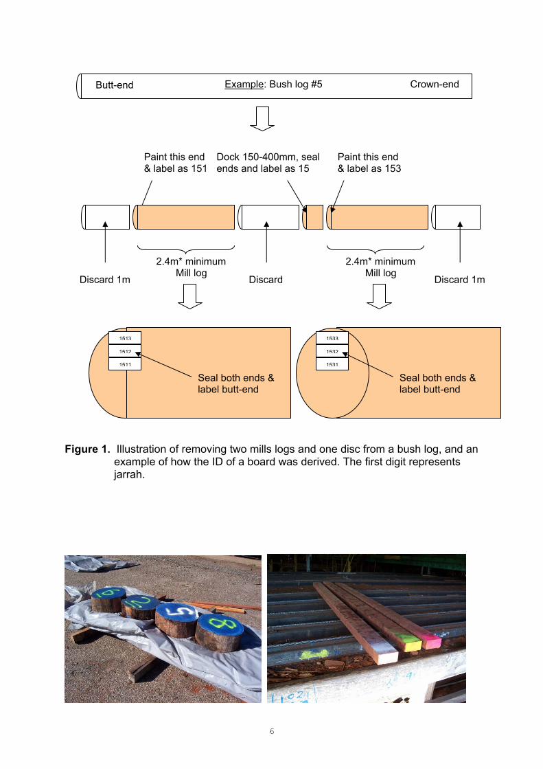
Figure 1. Illustration of removing two mills logs and one disc from a bush log, and an
example of how the ID of a board was derived. The first digit represents jarrah.
1513
1512
1511
Seal both ends & label butt-end
1533
1532
1531
Seal both ends & label butt-end
2.4m* minimum Mill log
Paint this end & label as 151
Discard 1m Discard 1m Discard
Example: Bush log #5
Paint this end & label as 153
Dock 150-400mm, seal ends and label as 15
Butt-end Crown-end
2.4m* minimum Mill log

7
Figure 2. The discs were end sealed and marked. Three boards were cut from the inner, mid and outer locations of a mill log (jarrah).
Figure 3. Log cutting to obtain sawn boards for study (E. nitens).
8
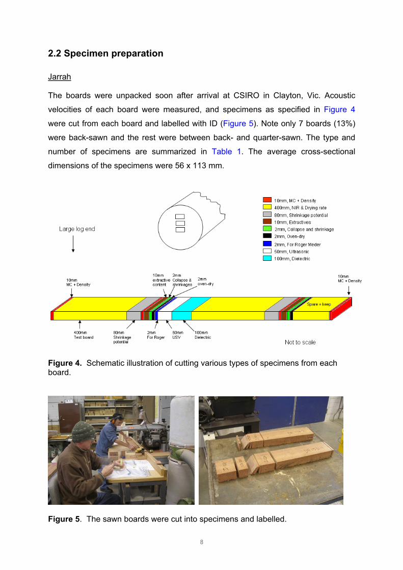
2.2 Specimen preparation Jarrah The boards were unpacked soon after arrival at CSIRO in Clayton, Vic. Acoustic
velocities of each board were measured, and specimens as specified in Figure 4
were cut from each board and labelled with ID (Figure 5). Note only 7 boards (13%)
were back-sawn and the rest were between back- and quarter-sawn. The type and
number of specimens are summarized in Table 1. The average cross-sectional
dimensions of the specimens were 56 x 113 mm.
Figure 4. Schematic illustration of cutting various types of specimens from each board.
Figure 5. The sawn boards were cut into specimens and labelled.
9
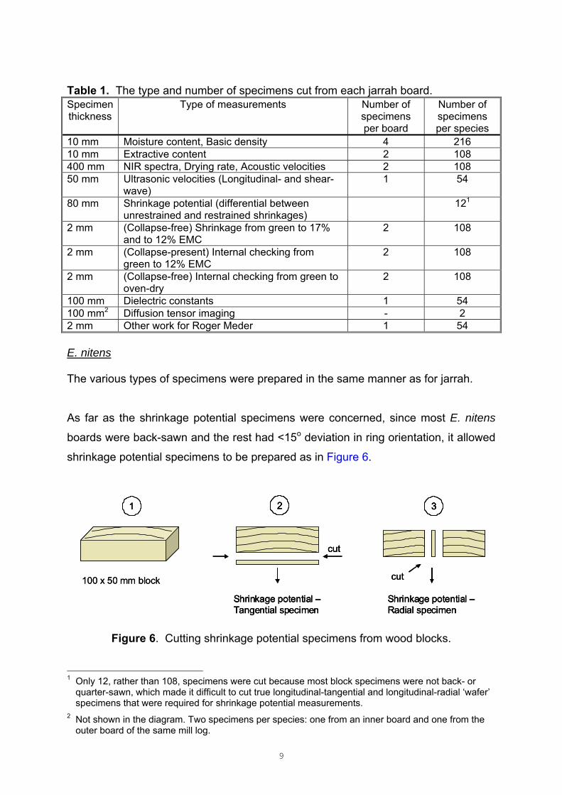
Table 1. The type and number of specimens cut from each jarrah board. Specimen thickness
Type of measurements Number of specimens per board
Number of specimens per species
10 mm Moisture content, Basic density 4 216 10 mm Extractive content 2 108 400 mm NIR spectra, Drying rate, Acoustic velocities 2 108 50 mm Ultrasonic velocities (Longitudinal- and shear-
wave) 1 54
80 mm Shrinkage potential (differential between unrestrained and restrained shrinkages)
121
2 mm (Collapse-free) Shrinkage from green to 17% and to 12% EMC
2 108
2 mm (Collapse-present) Internal checking from green to 12% EMC
2 108
2 mm (Collapse-free) Internal checking from green to oven-dry
2 108
100 mm Dielectric constants 1 54 100 mm2 Diffusion tensor imaging - 2 2 mm Other work for Roger Meder 1 54 E. nitens The various types of specimens were prepared in the same manner as for jarrah.
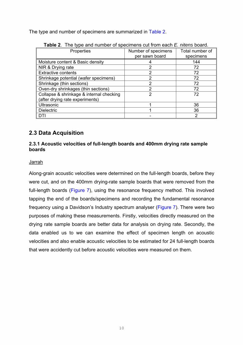
As far as the shrinkage potential specimens were concerned, since most E. nitens
boards were back-sawn and the rest had <15o deviation in ring orientation, it allowed
shrinkage potential specimens to be prepared as in Figure 6.
100 x 50 mm block
1 3
Shrinkage potential –Radial specimen
cut
2
Shrinkage potential –Tangential specimen
cut
100 x 50 mm block
11 3
Shrinkage potential –Radial specimen
cut
33
Shrinkage potential –Radial specimen
cut
2
Shrinkage potential –Tangential specimen
cut
22
Shrinkage potential –Tangential specimen
cut
Figure 6. Cutting shrinkage potential specimens from wood blocks. 1 Only 12, rather than 108, specimens were cut because most block specimens were not back- or
quarter-sawn, which made it difficult to cut true longitudinal-tangential and longitudinal-radial ‘wafer’ specimens that were required for shrinkage potential measurements.
2 Not shown in the diagram. Two specimens per species: one from an inner board and one from the outer board of the same mill log.
10
The type and number of specimens are summarized in Table 2.
Table 2. The type and number of specimens cut from each E. nitens board.
Properties Number of specimens per sawn board
Total number of specimens
Moisture content & Basic density 4 144 NIR & Drying rate 2 72 Extractive contents 2 72 Shrinkage potential (wafer specimens) 2 72 Shrinkage (thin sections) 2 72 Oven-dry shrinkages (thin sections) 2 72 Collapse & shrinkage & internal checking (after drying rate experiments)
2 72
Ultrasonic 1 36 Dielectric 1 36 DTI - 2
2.3 Data Acquisition
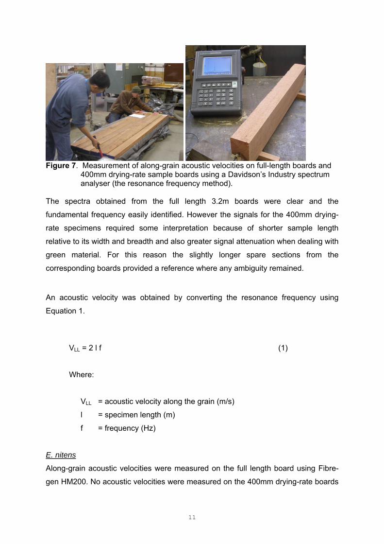
2.3.1 Acoustic velocities of full-length boards and 400mm drying rate sample boards Jarrah Along-grain acoustic velocities were determined on the full-length boards, before they
were cut, and on the 400mm drying-rate sample boards that were removed from the
full-length boards (Figure 7), using the resonance frequency method. This involved
tapping the end of the boards/specimens and recording the fundamental resonance
frequency using a Davidson’s Industry spectrum analyser (Figure 7). There were two
purposes of making these measurements. Firstly, velocities directly measured on the
drying rate sample boards are better data for analysis on drying rate. Secondly, the
data enabled us to we can examine the effect of specimen length on acoustic
velocities and also enable acoustic velocities to be estimated for 24 full-length boards
that were accidently cut before acoustic velocities were measured on them.
11
Figure 7. Measurement of along-grain acoustic velocities on full-length boards and
400mm drying-rate sample boards using a Davidson’s Industry spectrum analyser (the resonance frequency method).
The spectra obtained from the full length 3.2m boards were clear and the
fundamental frequency easily identified. However the signals for the 400mm drying-
rate specimens required some interpretation because of shorter sample length
relative to its width and breadth and also greater signal attenuation when dealing with
green material. For this reason the slightly longer spare sections from the
corresponding boards provided a reference where any ambiguity remained.
An acoustic velocity was obtained by converting the resonance frequency using
Equation 1.
VLL = 2 l f (1)
Where:
VLL = acoustic velocity along the grain (m/s)
l = specimen length (m)
f = frequency (Hz)
E. nitens
Along-grain acoustic velocities were measured on the full length board using Fibre-
gen HM200. No acoustic velocities were measured on the 400mm drying-rate boards
12
because the Davidson’s Industry spectrum analyser became dysfunctional and
400mm is too short for Fibre-gen HM200.
2.3.2 Near infra-red (NIR) spectroscopy
Jarrah and E. nitens
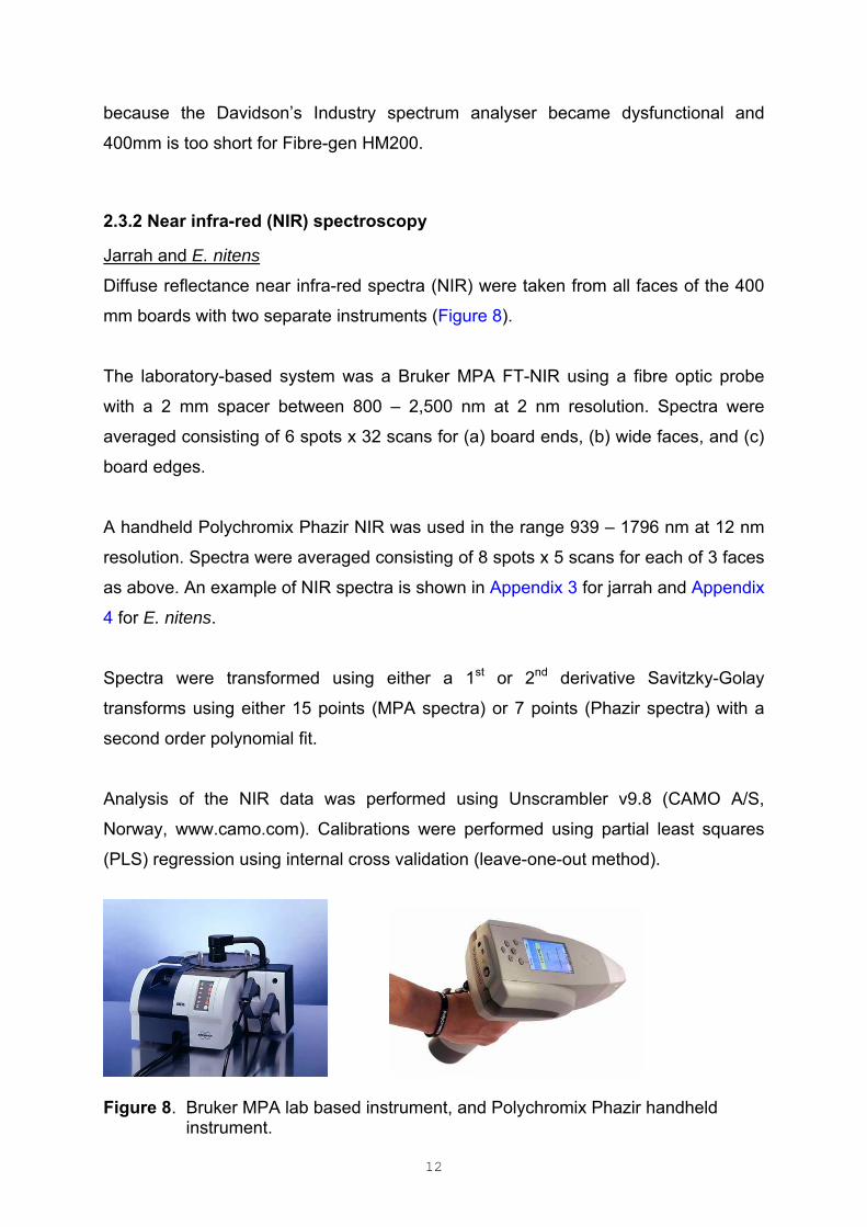
Diffuse reflectance near infra-red spectra (NIR) were taken from all faces of the 400
mm boards with two separate instruments (Figure 8).
The laboratory-based system was a Bruker MPA FT-NIR using a fibre optic probe
with a 2 mm spacer between 800 – 2,500 nm at 2 nm resolution. Spectra were
averaged consisting of 6 spots x 32 scans for (a) board ends, (b) wide faces, and (c)
board edges.
A handheld Polychromix Phazir NIR was used in the range 939 – 1796 nm at 12 nm
resolution. Spectra were averaged consisting of 8 spots x 5 scans for each of 3 faces
as above. An example of NIR spectra is shown in Appendix 3 for jarrah and Appendix
4 for E. nitens.
Spectra were transformed using either a 1st or 2nd derivative Savitzky-Golay
transforms using either 15 points (MPA spectra) or 7 points (Phazir spectra) with a
second order polynomial fit.
Analysis of the NIR data was performed using Unscrambler v9.8 (CAMO A/S,
Norway, www.camo.com). Calibrations were performed using partial least squares
(PLS) regression using internal cross validation (leave-one-out method).
Figure 8. Bruker MPA lab based instrument, and Polychromix Phazir handheld
instrument.
13
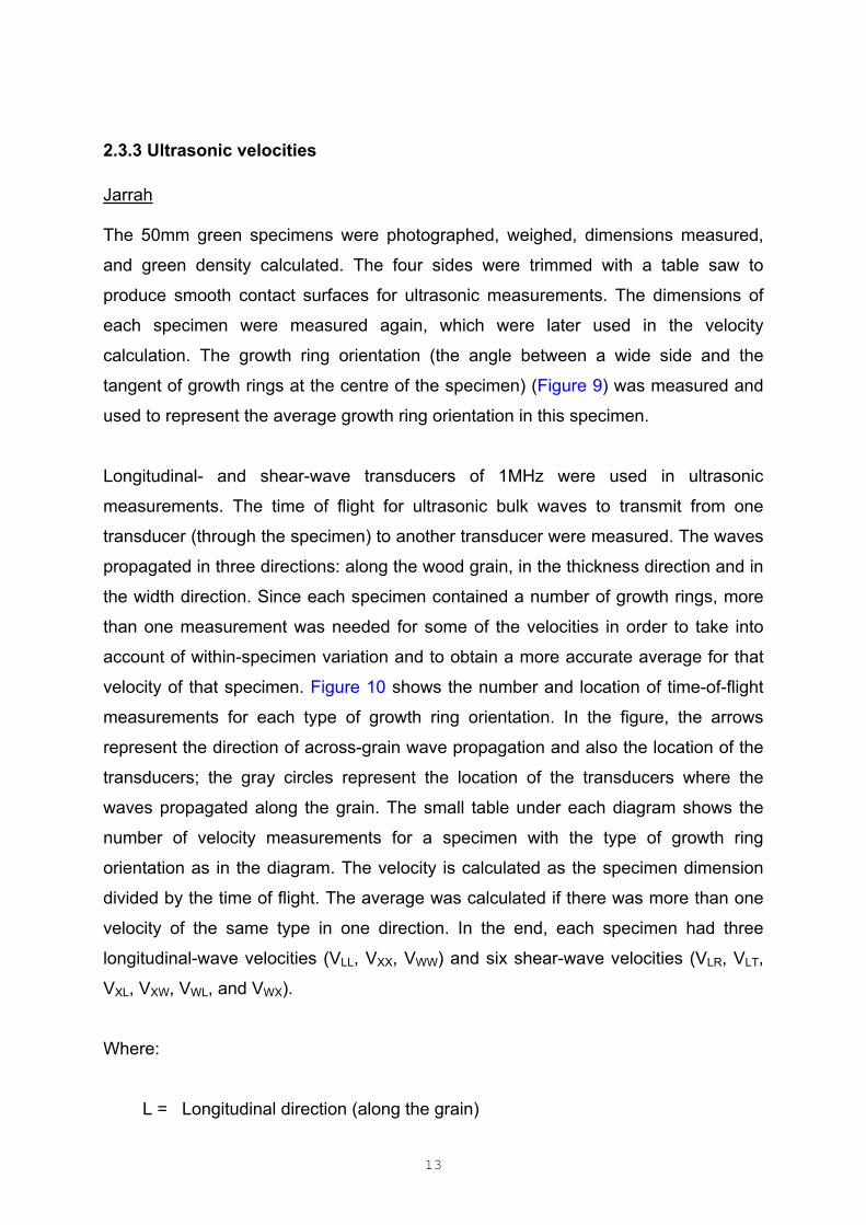
2.3.3 Ultrasonic velocities Jarrah The 50mm green specimens were photographed, weighed, dimensions measured,
and green density calculated. The four sides were trimmed with a table saw to
produce smooth contact surfaces for ultrasonic measurements. The dimensions of
each specimen were measured again, which were later used in the velocity
calculation. The growth ring orientation (the angle between a wide side and the
tangent of growth rings at the centre of the specimen) (Figure 9) was measured and
used to represent the average growth ring orientation in this specimen.
Longitudinal- and shear-wave transducers of 1MHz were used in ultrasonic
measurements. The time of flight for ultrasonic bulk waves to transmit from one
transducer (through the specimen) to another transducer were measured. The waves
propagated in three directions: along the wood grain, in the thickness direction and in
the width direction. Since each specimen contained a number of growth rings, more
than one measurement was needed for some of the velocities in order to take into
account of within-specimen variation and to obtain a more accurate average for that
velocity of that specimen. Figure 10 shows the number and location of time-of-flight
measurements for each type of growth ring orientation. In the figure, the arrows
represent the direction of across-grain wave propagation and also the location of the
transducers; the gray circles represent the location of the transducers where the
waves propagated along the grain. The small table under each diagram shows the
number of velocity measurements for a specimen with the type of growth ring
orientation as in the diagram. The velocity is calculated as the specimen dimension
divided by the time of flight. The average was calculated if there was more than one
velocity of the same type in one direction. In the end, each specimen had three
longitudinal-wave velocities (VLL, VXX, VWW) and six shear-wave velocities (VLR, VLT,
VXL, VXW, VWL, and VWX).
Where:
L = Longitudinal direction (along the grain)

14
R = Radial direction
T = Tangential direction
X = In the thickness direction
W = In the width direction
The VXX and VWW values were then corrected by using the mean VRR and VTT values
of the 7 back-sawn specimens as the long- and short-axis of the ellipse respectively,
assuming across-grain longitudinal velocities vary with growth ring orientation and
follow an elliptical distribution. The VXW and VWX did not need correction1. The
velocity data are summarized in
Appendix 5.
Reference Reference
Figure 9. The angle of growth ring orientation at the centre of a specimen.
1 Personal communication with Dr. Grant Emms of Scion, New Zealand.

15
Back-sawn quarter-sawn
In-between (more towards back-sawn)
21
3 123
In-between (more towards quarter-sawn)
Specimen width
Spe
cim
en
thic
knes
s
21
3 3 2 1
Velocity VLL VXX VWW VLX VLW VXL VXW VWL VWX
No. of measure. 3 1 1 3 3 1 1 1 1Velocity VLL VXX VWW VLX VLW VXL VXW VWL VWX
No. of measure. 3 1 3 3 3 1 1 3 3
Velocity VLL VXX VWW VLX VLW VXL VXW VWL VWX
No. of measure. 3 1 1 3 3 1 1 1 1Velocity VLL VXX VWW VLX VLW VXL VXW VWL VWX
No. of measure. 3 1 3 3 3 1 1 3 3
Back-sawn quarter-sawn
In-between (more towards back-sawn)
21
321
3 123 123
In-between (more towards quarter-sawn)
Specimen width
Spe
cim
en
thic
knes
s
21
321
3 3 2 13 2 1
Velocity VLL VXX VWW VLX VLW VXL VXW VWL VWX
No. of measure. 3 1 1 3 3 1 1 1 1Velocity VLL VXX VWW VLX VLW VXL VXW VWL VWX
No. of measure. 3 1 3 3 3 1 1 3 3
Velocity VLL VXX VWW VLX VLW VXL VXW VWL VWX
No. of measure. 3 1 1 3 3 1 1 1 1Velocity VLL VXX VWW VLX VLW VXL VXW VWL VWX
No. of measure. 3 1 3 3 3 1 1 3 3 Figure 10. Illustration of the number and location of ultrasonic measurements in four
types of growth ring orientations. E. nitens Most E. nitens boards were back-sawn and the rest had <15o deviation in ring
orientation. For this reason, and also based on observations on ultrasonic
measurements on jarrah, only one measurement of each type of ultrasonic velocities
was made on each specimen. Two shear wave velocities (VWL and VWT), however,
cannot be obtained because the instrument can barely detect the ultrasonic signals
given the width and moisture content of the specimens. We did not make an attempt
to resize the specimen width because that would change physical composition of the
specimens and also because VWL and VWT are less likely measured in practice as far
as sawn boards are concerned. The velocity data are summarized in Appendix 6.
16
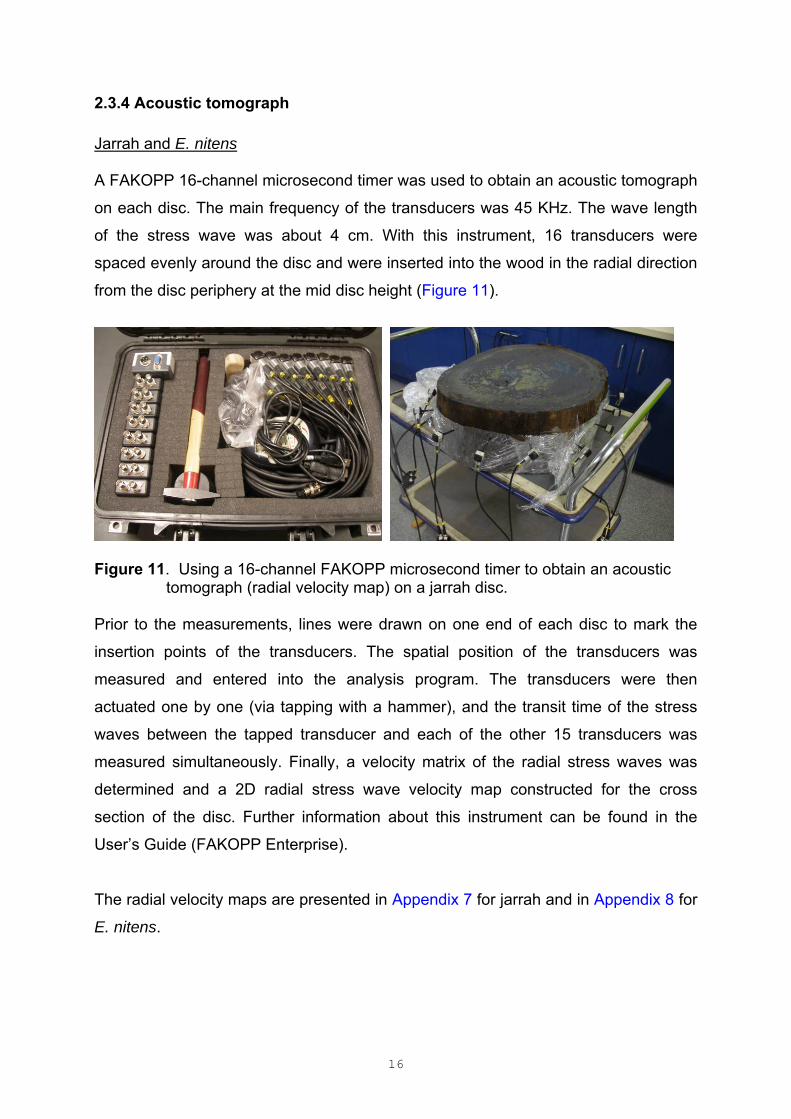
2.3.4 Acoustic tomograph Jarrah and E. nitens A FAKOPP 16-channel microsecond timer was used to obtain an acoustic tomograph
on each disc. The main frequency of the transducers was 45 KHz. The wave length
of the stress wave was about 4 cm. With this instrument, 16 transducers were
spaced evenly around the disc and were inserted into the wood in the radial direction
from the disc periphery at the mid disc height (Figure 11).
Figure 11. Using a 16-channel FAKOPP microsecond timer to obtain an acoustic
tomograph (radial velocity map) on a jarrah disc. Prior to the measurements, lines were drawn on one end of each disc to mark the
insertion points of the transducers. The spatial position of the transducers was
measured and entered into the analysis program. The transducers were then
actuated one by one (via tapping with a hammer), and the transit time of the stress
waves between the tapped transducer and each of the other 15 transducers was
measured simultaneously. Finally, a velocity matrix of the radial stress waves was
determined and a 2D radial stress wave velocity map constructed for the cross
section of the disc. Further information about this instrument can be found in the
User’s Guide (FAKOPP Enterprise).
The radial velocity maps are presented in Appendix 7 for jarrah and in Appendix 8 for
E. nitens.

17
2.3.5 Dielectric property measurements The measurements were carried out at the Petrophysics Laboratory of the CSIRO
Division of Earth Science and Resource Engineering (CESRE) in Perth.
End loaded coaxial lines (Burdette, Cain and Seals 1980; Stuchly and Stuchly 1980;
Figure 12; Figure 13) are commonly used for measuring dielectric constants in
materials in the range from ~10MHz up to above 3GHz, while suitably sized open
ended coaxial probes may allow measurements as low as 100 kHz to be achieved. In
this procedure a wave is transmitted along the transmission line towards the sample,
where the difference in propagation parameters of the sample causes a reflection to
propagate back up the transmission line. The Petrophysics Laboratory at Australian
Resources Research Centre (ARRC) in Kensington, WA uses a slightly larger
diameter version of the commercially available system to allow larger area samples
(such as the boards in this study) to be analysed. The system is connected to an
Agilent 5070 network vector analyser to determine the reflection S-parameter which
is then used to compute the real and imaginary dielectric constant. In this study the
frequency range was 300 kHz to 3 GHz.
Figure 12. End-loaded coaxial line suitable for obtaining material dielectric
properties (real permittivity and loss) using reflection coefficient
measurements with a vector network analyzer. The region of investigation
is limited to the vicinity of the probe end. Air gaps must be avoided at the
sample interface.
r
18
Figure 13. Photograph of the end-loaded transmission line probe.
Sample Preparation The wood samples as received were wrapped tight in cling film and separately
bagged in individual zip lock bags. On receipt at the ARRC they were stored in a cold
room in order to maintain their true in-situ moisture content. This was necessary to
ensure that the dielectric response wasn’t severely altered (dielectric response is
strongly affected by moisture). Prior to analysis the samples were allowed to
equilibrate in the laboratory at 24 °C for 2 days to achieve a constant temperature for
all the samples. The samples had approximately 5 mm of material planed off them, to
provide a fresh flat surface suitable for the endloaded probe. The shavings were
weighed before and after drying at 50 °C to determine the moisture content.
2.3.6 Diffusion tensor imaging Background
The movement of water in wood is related to the porosity of the wood matrix which.
Under ambient conditions water self-diffuses according to Einstein’s Theory of
Brownian motion (Einstein 1905). Barriers to water self-diffusion arise from changes
in the wood permeability, due in turn to changes in wood anatomy, particularly within
and between annual rings. Changes in the permeability of wood have previously
been studied and modeled in order to explain the drying behaviour (Booker, 1990;
Pang and Wiberg, 1998). The drying process simply amplifies the rate of molecular
self-diffusion by applying a temperature gradient a cross the wood. An increase in
temperature from 25 °C to 100 °C increases the rate of diffusion approximately 37-
fold (Stamm 1964).

19
Measurement of the self-diffusion of water in situ is however difficult to perform.
Magnetic resonance imaging (MRI) does offer one means of determining the
magnitude of diffusion via MR diffusion tensor imaging (DTI). This allows the
anisotropy of diffusion to be visualised in terms of the direction(s) of greatest and
least restriction to diffusion with respect to the sample orientation, at ambient
conditions along with the magnitude of the diffusion. Diffusion tensor imaging has
previously been used to visualise restricted diffusion in highly anisotropic materials
such as the eye lens (Moffat and Pope, 2002), wood (Meder et al., 2003b) and
cartilage (Meder et al., 2006).
Diffusion tensor imaging (LeBihan, 1991; Basser et al., 1994) is an MRI technique to
determine the direction and magnitude of molecular self diffusion and is used
routinely to track fibres in the brain. The MRI signal is sensitised to diffusion by
judicial selection of the diffusion time according to the Einstein equation,
2D t (Einstein, 1905), so that the mean displacement is bounded by the known
dimension of the element to be studied, in this case the cell dimensions. Calculation
of the diffusion tensor describes the three orthogonal directions in terms of their
increasing resistance to. This in turn can be interpreted as tracing the wood fibres
along their long and short axes with the long axis offering least resistance to diffusion
while the short axis being most hindered. In this manner it is also possible to
determine the magnitude of diffusion and by extension the relative diffusivity at any
location in the sample cross section.
When diffusion is anisotropic as can be expected to occur in the structurally aligned
wood architecture, the self-diffusion of the water protons must be characterised by a
3 x 3 tensor, describing both the magnitude and direction of the diffusion in 3-
dimensional space.
Methodology
The diffusion tensor was determined in a selection of the end-matched boards based
on previously obtained data (board USV, NIR, MC profile and extractives content) to
ensure a broad range of property variation is achieved. From the diffusion tensor the
Eigenvectors (direction(s) of least restricted and most restricted diffusion) and their

20
corresponding Eigenvalues (magnitude of diffusion along the direction of the three
orthogonal Eigenvectors) were obtained.
All MR imaging was performed on a Siemens Sonata 3T clinical MRI system using a
16 channel head coil. Pairs of boards (inner and outer boards from individual logs)
were sealed in polyurethane film prior to imaging. The head coil provided sufficient
room to accommodate two pairs of boards for each imaging run. An initial localiser
image was performed to ensure the imaging plane for the DTI study was centred in
the boards. Diffusion tensor imaging was performed with the following imaging
parameters:
Data matrix size, MTX: 512x512 pixels
Field of view, FOV: ~500x600 mm
In-plane resolution: ~1x1 mm
Slice Thickness, THK: 6 mm
Number of averages, NA: 32
Orientation of diffusion gradient directions:
Read = Radial
Phase = Longitudinal
Slice = Tangential
Diffusion gradient magnitudes, b:
E. nitens: 0, 100, 200, 400, 1000, 2000, 5,000, 10,000
E. marginata: 0, 50, 100, 200, 500, 800, 1,000
Echo time, TE:
E. nitens: 175 ms
E. marginata: 96 ms
Repetition time, TR: 500 ms
2.3.7 Moisture content and basic density Jarrah and E. nitens
21
Moisture content and basic density were determined using the 10mm specimens.
The volume of the oven-dried wood blocks was measured with the water immersion
method. The data are given in Appendix 9 for jarrah and in Appendix 10 for E. nitens.
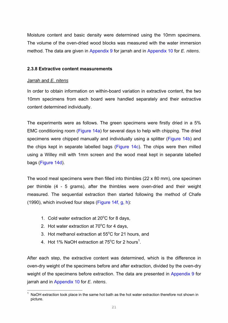
2.3.8 Extractive content measurements Jarrah and E. nitens In order to obtain information on within-board variation in extractive content, the two
10mm specimens from each board were handled separately and their extractive
content determined individually.
The experiments were as follows. The green specimens were firstly dried in a 5%
EMC conditioning room (Figure 14a) for several days to help with chipping. The dried
specimens were chipped manually and individually using a splitter (Figure 14b) and
the chips kept in separate labelled bags (Figure 14c). The chips were then milled
using a Willey mill with 1mm screen and the wood meal kept in separate labelled
bags (Figure 14d).
The wood meal specimens were then filled into thimbles (22 x 80 mm), one specimen
per thimble (4 - 5 grams), after the thimbles were oven-dried and their weight
measured. The sequential extraction then started following the method of Chafe
(1990), which involved four steps (Figure 14f, g, h):
1. Cold water extraction at 20oC for 8 days,
2. Hot water extraction at 70oC for 4 days,
3. Hot methanol extraction at 55oC for 21 hours, and
4. Hot 1% NaOH extraction at 75oC for 2 hours1.
After each step, the extractive content was determined, which is the difference in
oven-dry weight of the specimens before and after extraction, divided by the oven-dry
weight of the specimens before extraction. The data are presented in Appendix 9 for
jarrah and in Appendix 10 for E. nitens.
1 NaOH extraction took place in the same hot bath as the hot water extraction therefore not shown in
picture.

22
(a) 10mm block specimens were being dried (b) Manually chipping a 10mm block specimen
(c) Specimens in the form of wood chips (d) Specimens in the form of wood meal
(e) Thimbles for holding wood meals (f) Specimens in cold water extraction

23
(g) Specimens in hot water extraction (h) Specimens in methanol extraction
(i) Specimens in hot NaOH extraction (j) Specimens after NaOH extraction Figure 14. The process of determining extractive contents in jarrah block specimens.
2.3.9 Drying rate Jarrah Drying rates were determined on the end-matched 400mm sample boards (one pair
of end-matched sample boards were cut from each sawn board, Figure 4). The
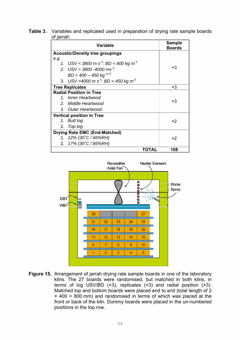
sampling of the drying rate boards allowed for the following variables (Table 3).
One board from each pair of end-matched boards was randomly allocated to one of
the two laboratory kilns, which were set with an equilibrium moisture content of either
17% or 12% moisture content. The dimensions of the timber stack that can be placed
in the kilns are 550 mm (wide) × 415 mm (high) × 800 mm (deep). Hence, two
sample boards were arranged end to end (2 × 400 = 800 mm). In this case the
boards were matched for height in the tree. The height boards were placed in front or
back randomly. The arrangement of the sample boards is shown diagrammatically in
Figure 15.
24
Table 3. Variables and replicated used in preparation of drying rate sample boards of jarrah.
Variable Sample Boards
Acoustic/Density tree groupings e.g.
1. USV < 3800 m s-1: BD < 400 kg m-3 2. USV = 3800 -4000 ms-1:
BD = 400 – 450 kg m-3 3. USV >4000 m s-1: BD > 450 kg m-3
×3
Tree Replicates ×3 Radial Position in Tree
1. Inner Heartwood 2. Middle Heartwood 3. Outer Heartwood
×3
Vertical position in Tree 1. Butt log 2. Top log
×2
Drying Rate EMC (End-Matched) 1. 12% (30˚C / 66%RH) 2. 17% (30˚C / 85%RH)
×2
TOTAL 108
Figure 15. Arrangement of jarrah drying rate sample boards in one of the laboratory kilns. The 27 boards were randomised, but matched in both kilns, in terms of log USV/BD (×3), replicates (×3) and radial position (×3). Matched top and bottom boards were placed end to end (total length of 2 × 400 = 800 mm) and randomised in terms of which was placed at the front or back of the kiln. Dummy boards were placed in the un-numbered positions in the top row.

25
The green boards were weighed prior to drying, on the 4th day after the drying
commenced, then weighed again one week later, and again once every fortnight until
the change in weight became negligible. Each time the boards were weighed, the
width and thickness were also measured at locations A and B in each board, which
was 1/3 of the length of the board from each board end.
After the drying ended, one 2mm-thick thin section was cut from the location A of
each board. These sections were weighed immediately. Measurements on internal
checking and collapse were made soon afterwards using an imaging method as
described in the next section. The thin sections were then oven-dried, weighted and
the moisture content calculated which would represent the moisture content of the
sample boards at the time the drying ended. These moisture content values were
used to calculate Time Constant and to adjust the measured shrinkage and collapse
values to those at 12%.
From the weight measurements and the moisture contents of the sample boards, the
Time Constant was calculated. The relationships between the percentage change in
moisture content and Time Constant are given in Table 4 and also illustrated in
Figure 16.
Table 4. Time Constant Values (ASTM D 4933). Time Constant Percentage change
1 63.2 2 86 3 95 4 98 5 99

26
Figure 16. Plot of relationship between Percentage of Change and Time Constant values in Table 4.
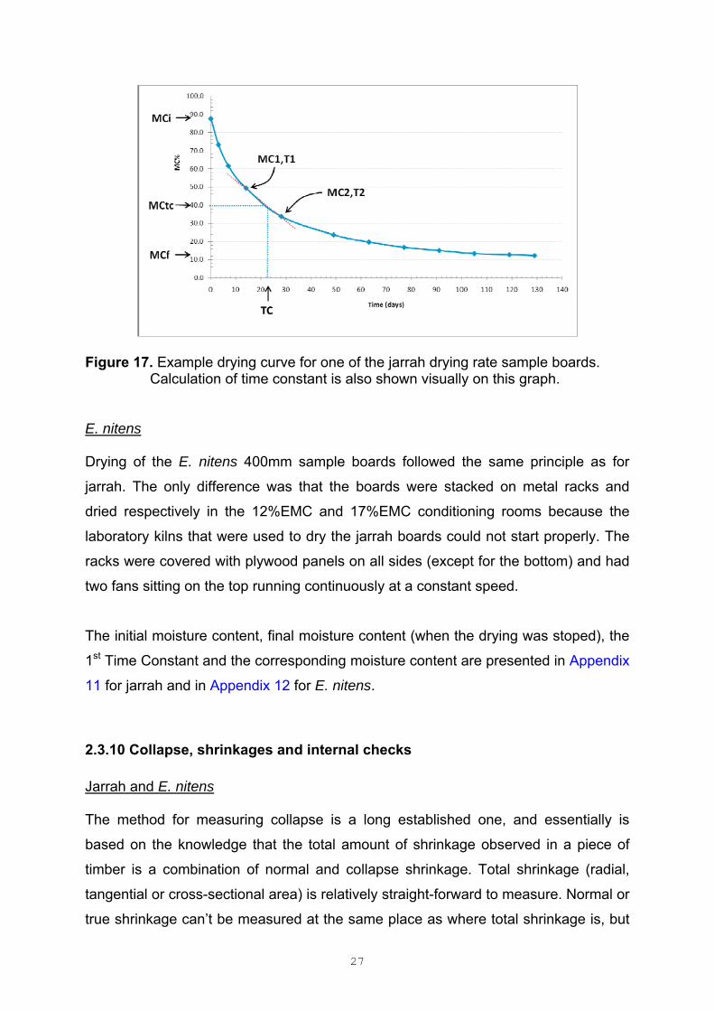
Below is an example of the calculation for the board shown in Figure 17:
MCtc = MCi + 0.632(MCf - MCi) Equation 1
i.e. 87.5 + 0.632(12.3 - 87.5) = 40.0%
Where:
MCtc = Moisture Content Value atone time constant
MCi = Initial Moisture Content
MCf = Final Moisture Content (EMC)
A linear interpolation was then used to calculate the time constant corresponding to
this moisture content (T1, T2, MC1 and MC2 are shown on Figure 17).
TC = T1 + (MCtc – MC1) × (T2 – T1) / (MC2 - MC1) Equation 2
i.e. 14 + (40.0 - 49.4) × (28 - 14)/(33.8 - 49.4) = 22.4 days
27
Figure 17. Example drying curve for one of the jarrah drying rate sample boards.
Calculation of time constant is also shown visually on this graph. E. nitens Drying of the E. nitens 400mm sample boards followed the same principle as for
jarrah. The only difference was that the boards were stacked on metal racks and
dried respectively in the 12%EMC and 17%EMC conditioning rooms because the
laboratory kilns that were used to dry the jarrah boards could not start properly. The
racks were covered with plywood panels on all sides (except for the bottom) and had
two fans sitting on the top running continuously at a constant speed.
The initial moisture content, final moisture content (when the drying was stoped), the
1st Time Constant and the corresponding moisture content are presented in Appendix
11 for jarrah and in Appendix 12 for E. nitens.
2.3.10 Collapse, shrinkages and internal checks Jarrah and E. nitens The method for measuring collapse is a long established one, and essentially is
based on the knowledge that the total amount of shrinkage observed in a piece of
timber is a combination of normal and collapse shrinkage. Total shrinkage (radial,
tangential or cross-sectional area) is relatively straight-forward to measure. Normal or
true shrinkage can’t be measured at the same place as where total shrinkage is, but
28
a reasonable measure can be obtained from a nearby section of wood. The true or
normal shrinkage is measured on a thin (1.5 mm thick – longitudinal direction) cross-
sectional section cut from the ends of the sample board. As eucalypt fibres are
1.1mm on average, it is reasonable to assume that there are no intact fibres in the
thin sections. If there are no intact fibres it is not possible for hydrostatic tension to be
present, and hence no collapse can occur. The relationship between normal and total
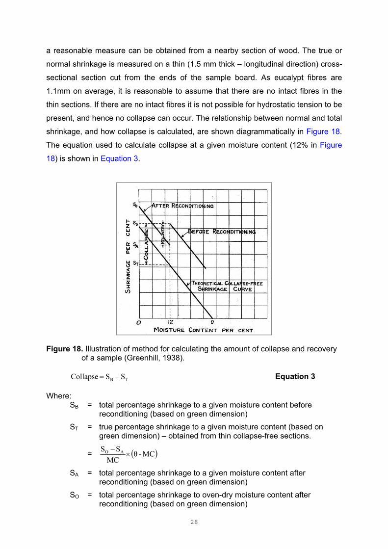
shrinkage, and how collapse is calculated, are shown diagrammatically in Figure 18.
The equation used to calculate collapse at a given moisture content (12% in Figure
18) is shown in Equation 3.
Figure 18. Illustration of method for calculating the amount of collapse and recovery of a sample (Greenhill, 1938).
TB SSCollapse Equation 3 Where:
SB = total percentage shrinkage to a given moisture content before reconditioning (based on green dimension)
ST = true percentage shrinkage to a given moisture content (based on green dimension) – obtained from thin collapse-free sections.
= MC-θMC
SS AO
SA = total percentage shrinkage to a given moisture content after reconditioning (based on green dimension)
SO = total percentage shrinkage to oven-dry moisture content after reconditioning (based on green dimension)
29
MC = moisture content
θ = intersection point (in percentage moisture content) for the type of shrinkage concerned
In this study, two types of specimens were used to generate the measurements
needed for determining shrinkage and collapse. The specimens were the 2mm thin
sections for collapse-free shrinkage, and the 2mm thin sections removed from the
400mm drying rate sample boards after the drying ended. The measurements were
collapse-free shrinkage, total collapse shrinkage, unit shrinkage rate, and moisture
content of the specimens.
Collapse-free shrinkage and unit shrinkages were obtained from the 2mm thin
collapse-free shrinkage specimens. The specimens were dried from green to 17%
MC (in 17%EMC room), then to 12% MC (in 12% EMC room), and then to 5% MC (in
5% EMC room). At green and at each other moisture content, the specimens were
weighed, the width and thickness measured using a Vernier digital calliper, and the
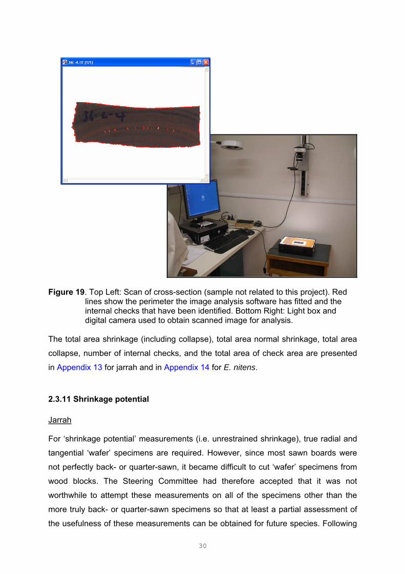
cross-sectional area measured by scanning the outline of the sections into a PC
based image analysis package (IMAGE PRO PLUS) (Figure 19). From these
measurements, collapse-free shrinkage from green to 12%MC (width, thickness,
cross-sectional area), and collapse-free unit shrinkage (width, thickness, area) were
then calculated.
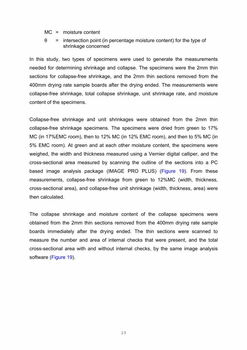
The collapse shrinkage and moisture content of the collapse specimens were
obtained from the 2mm thin sections removed from the 400mm drying rate sample
boards immediately after the drying ended. The thin sections were scanned to
measure the number and area of internal checks that were present, and the total
cross-sectional area with and without internal checks, by the same image analysis
software (Figure 19).
30
Figure 19. Top Left: Scan of cross-section (sample not related to this project). Red
lines show the perimeter the image analysis software has fitted and the internal checks that have been identified. Bottom Right: Light box and digital camera used to obtain scanned image for analysis.
The total area shrinkage (including collapse), total area normal shrinkage, total area
collapse, number of internal checks, and the total area of check area are presented
in Appendix 13 for jarrah and in Appendix 14 for E. nitens.
2.3.11 Shrinkage potential Jarrah For ‘shrinkage potential’ measurements (i.e. unrestrained shrinkage), true radial and
tangential ‘wafer’ specimens are required. However, since most sawn boards were
not perfectly back- or quarter-sawn, it became difficult to cut ‘wafer’ specimens from
wood blocks. The Steering Committee had therefore accepted that it was not
worthwhile to attempt these measurements on all of the specimens other than the
more truly back- or quarter-sawn specimens so that at least a partial assessment of
the usefulness of these measurements can be obtained for future species. Following

31
the SC’s recommendation, 6 pairs of specimens were cut and the shrinkages in
radial and tangential directions from green to 12% EMC were determined. The data
are given in Appendix 15.
E. nitens
Most E. nitens sawn boards were back-sawn and a few remaining ones had growth
ring deviation less than 15 degrees. This enabled us to prepare the full set of ‘wafer’
specimens (i.e. two radial and two tangential specimens from each sawn board,
Figure 4). Radial and tangential dimensions of the specimens were measured in
green and at 12% MC, and the moisture contents were also determined. From these
measurements, radial and tangential shrinkage were determined, then adjusted to
those at 12% MC. The data are presented in Appendix 16.
2.3.12 Shrinkage in 2mm collapse-free sections (green to oven-dry)
Jarrah and E. nitens
The cross-sectional area of the green 2 mm sections was measured by scanning the
outline of the sections into a PC based image analysis package (IMAGE PRO
PLUS). The sections were then oven-dried and some restrain was applied to prevent
severe twisting or curling. The cross-sectional area in oven-dry condition was
measured using the same imaging method. The total cross-sectional area shrinkage
was calculated, and presented in Appendix 15 for jarrah and in Appendix 16 for E.
nitens.
2.3.13 Data Analysis
Forward Stepwise multiple regression was attempted to see which of the variables
have the most influence on drying rate (Time Constant), drying degrade (Internal
checking) and collapse.
32
These predictor variables include:
Wood properties
Initial moisture content
Green density, Basic density
Extractive contents
Log acoustic velocity
Sawn board acoustic velocity
400mm drying-rate sample boards (jarrah only)
Ultrasonic velocities
Shrinkage potential in radial and tangential directions
Shrinkage from green to oven-dry in radial and tangential directions and in
area
and other variables
Thickness of 400 mm drying-rate sample boards
Growth ring orientation (jarrah only)
As the ANOVA results show, the drying condition (between 12% and 17% kilns) had
significant effect on some dependant variables (i.e. drying rate and drying degrade)
and such effect was species dependant, the data set was then separated accordingly
into the 12% and 17% group for each species in corresponding regression analysis.
As expected, the drying condition did not affect collapse for both species as collapse
is strongly temperature dependent and the kilns were run at the same temperature.
In the jarrah regression analysis, several ultrasonic velocities are not included since it
is uncertain whether those velocities are reliable representation of VRR, VTT, VRL, VRT,
VTL and VTR due to original condition of the specimens, although corrections had
been done to some of them. Shrinkage potential is also not included because the
data are too few.
In the E. ntiens regression analysis, ultrasonic velocities VWL and VWX are not
included as the data were not obtained due to original condition of the specimens.
33
3. Results and Discussion
3.1. Assessment of drying rate and drying degrade
3.1.1 Drying rate
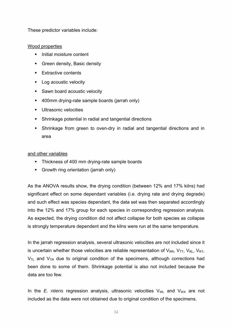
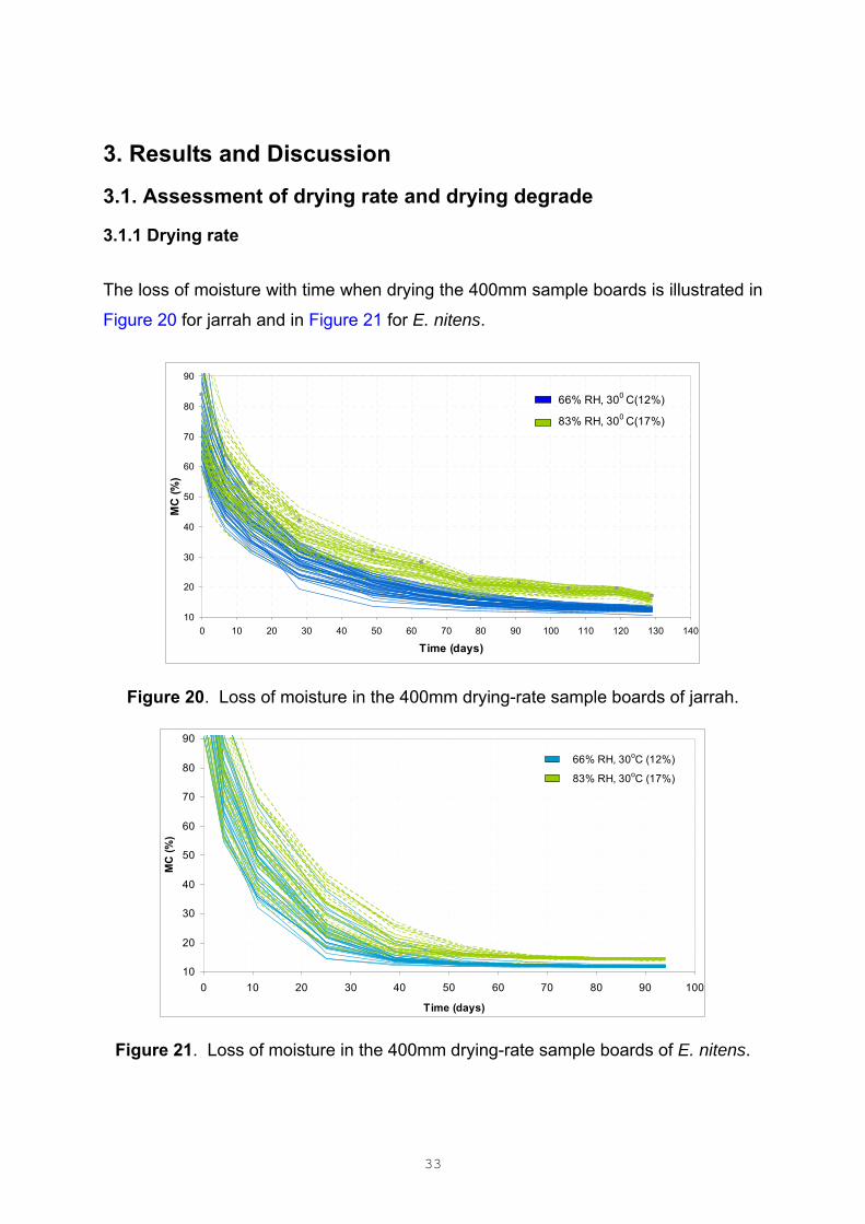
The loss of moisture with time when drying the 400mm sample boards is illustrated in
Figure 20 for jarrah and in Figure 21 for E. nitens.
10
20
30
40
50
60
70
80
90
0 10 20 30 40 50 60 70 80 90 100 110 120 130 140
Time (days)
MC
(%)
66% RH, 300 C(12%)
83% RH, 300 C(17%)
Figure 20. Loss of moisture in the 400mm drying-rate sample boards of jarrah.
10
20
30
40
50
60
70
80
90
0 10 20 30 40 50 60 70 80 90 100
Time (days)
MC
(%)
66% RH, 30oC (12%)
83% RH, 30oC (17%)
Figure 21. Loss of moisture in the 400mm drying-rate sample boards of E. nitens.
34
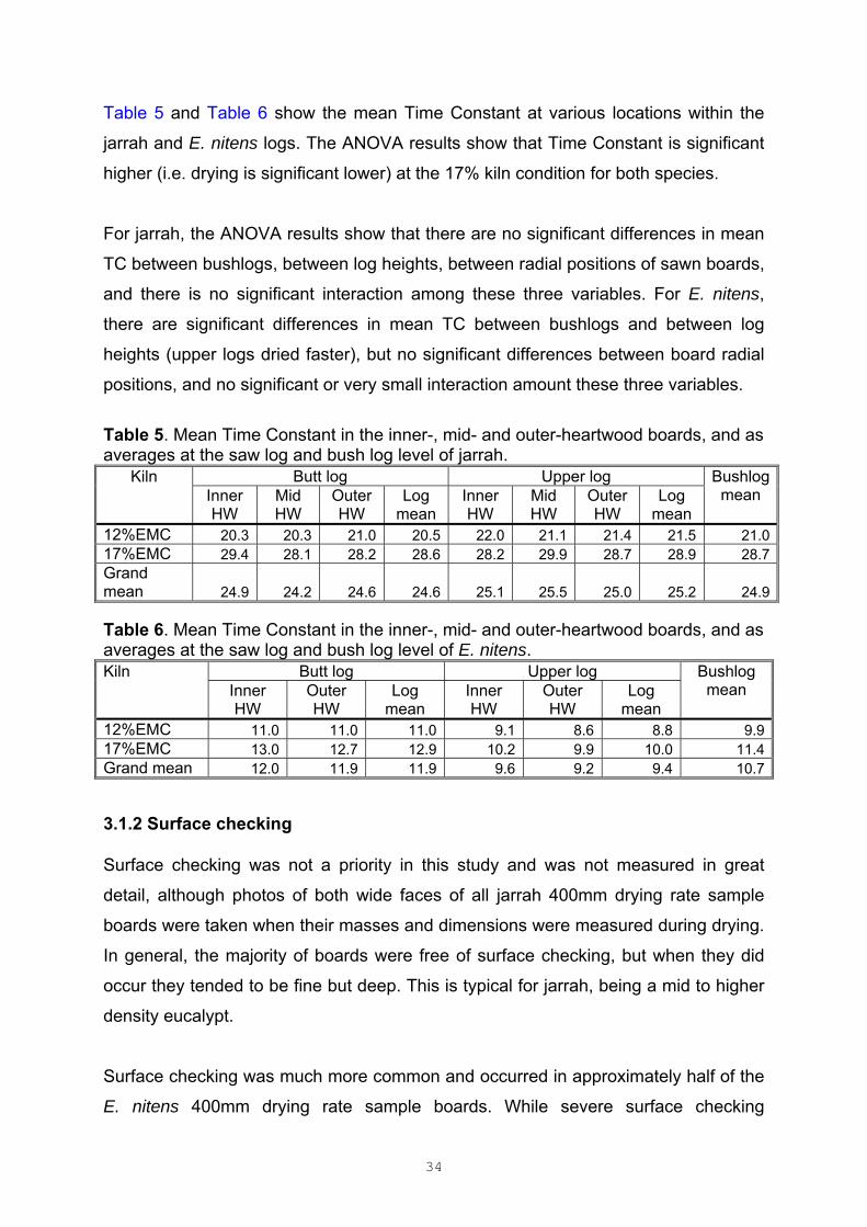
Table 5 and Table 6 show the mean Time Constant at various locations within the
jarrah and E. nitens logs. The ANOVA results show that Time Constant is significant
higher (i.e. drying is significant lower) at the 17% kiln condition for both species.
For jarrah, the ANOVA results show that there are no significant differences in mean
TC between bushlogs, between log heights, between radial positions of sawn boards,
and there is no significant interaction among these three variables. For E. nitens,
there are significant differences in mean TC between bushlogs and between log
heights (upper logs dried faster), but no significant differences between board radial
positions, and no significant or very small interaction amount these three variables.
Table 5. Mean Time Constant in the inner-, mid- and outer-heartwood boards, and as averages at the saw log and bush log level of jarrah.
Kiln Butt log Upper log Bushlog mean Inner
HW Mid HW
Outer HW
Log mean
Inner HW
Mid HW
Outer HW
Log mean
12%EMC 20.3 20.3 21.0 20.5 22.0 21.1 21.4 21.5 21.017%EMC 29.4 28.1 28.2 28.6 28.2 29.9 28.7 28.9 28.7Grand mean 24.9 24.2 24.6 24.6 25.1 25.5 25.0 25.2 24.9 Table 6. Mean Time Constant in the inner-, mid- and outer-heartwood boards, and as averages at the saw log and bush log level of E. nitens. Kiln Butt log Upper log Bushlog
mean Inner HW
Outer HW
Log mean
Inner HW
Outer HW
Log mean
12%EMC 11.0 11.0 11.0 9.1 8.6 8.8 9.917%EMC 13.0 12.7 12.9 10.2 9.9 10.0 11.4Grand mean 12.0 11.9 11.9 9.6 9.2 9.4 10.7
3.1.2 Surface checking Surface checking was not a priority in this study and was not measured in great
detail, although photos of both wide faces of all jarrah 400mm drying rate sample
boards were taken when their masses and dimensions were measured during drying.
In general, the majority of boards were free of surface checking, but when they did
occur they tended to be fine but deep. This is typical for jarrah, being a mid to higher
density eucalypt.
Surface checking was much more common and occurred in approximately half of the
E. nitens 400mm drying rate sample boards. While severe surface checking

35
developed in some sample boards, it was virtually free in several other sample
boards.
3.1.3 Collapse and internal checking – jarrah
Table 7 to Table 9 present mean values of collapse and internal checking measured
on jarrah 400mm drying rate sample boards. The ANOVA results show that
specimens in the 17% kiln condition had significant higher collapse but significantly
lower internal checking. Somewhat surprisingly collapse and internal checking were
generally greater higher up the tree. The area of checks was also higher up the tree
at the log level. The outer wood tended to have larger checked area.
Table 7. Mean number of internal checks in the inner-, mid- and outer-heartwood boards, and as averages at the saw log and bush log level of jarrah.
Kiln Butt log Upper log Bushlog mean Inner
HW Mid HW
Outer HW
Log mean
Inner HW
Mid HW
Outer HW
Log mean
12%EMC 3.4 5.0 3.8 4.1 5.4 6.0 7.2 6.2 5.1 17%EMC 1.9 5.0 2.2 3.0 2.9 2.4 3.1 2.8 2.9 Grand mean 2.7 5.0 3.0 3.6 4.2 4.2 5.2 4.5 4.0 Table 8. Mean area of checks (mm2) in the inner-, mid- and outer-heartwood boards, and as averages at the saw log and bush log level of jarrah.
Kiln Butt log Upper log Bushlog mean Inner
HW Mid HW
Outer HW
Log mean
Inner HW
Mid HW
Outer HW
Log mea
n 12%EMC 14.1 15.7 13.2 14.3 15.0 34.4 33.3 27.6 20.9 17%EMC 5.0 6.6 8.4 6.7 3.7 2.8 10.0 5.5 6.1 Grand mean 9.5 11.1 10.8 10.5 9.3 18.6 21.6 16.5 13.5 Table 9. Mean area collapse (%) in the inner-, mid- and outer-heartwood boards, and as averages at the saw log and bush log level of jarrah.
Kiln Butt log Upper log Bushlog mean Inner
HW Mid HW
Outer HW
Log mean
Inner HW
Mid HW
Outer HW
Log mean
12%EMC 12.1 10.7 8.7 10.5 13.7 14.7 12.1 13.5 12.0 17%EMC 12.8 14.0 9.9 12.2 16.6 16.0 10.1 14.2 13.2 Grand mean 12.5 12.3 9.3 11.4 15.1 15.4 11.1 13.9 12.6 Despite that internal checks developed in every log, the checking is considerably
milder in logs 2 and 4 at both heights than in others as shown in Table 10. At the

36
bushlog level, the number of checks and the total area of checks are closely
correlated as expected. The severity of internal checking (area of checks), however,
is not correlated to collapse. The best example is log 2, which had the highest total
area of checks but very low level of checking.
Table 10. Log means of collapse and internal checking of jarrah. Bushlog # Collapse (%) Number of checks Total checked area
(mm2) Lower log Upper log Lower log Upper log Lower log Upper log
1 10.08 12.02 5.7 6.5 20.05 22.702 16.38 16.10 1.2 1.0 1.63 6.923 11.83 17.45 7.5 10.5 20.87 31.454 4.78 4.80 2.5 0.2 3.12 0.905 13.13 14.70 5.3 4.3 12.35 10.996 10.15 18.53 1.3 4.8 2.37 19.017 10.73 12.02 4.3 6.7 15.76 13.648 15.67 15.27 0.7 1.7 4.20 10.819 9.47 13.83 3.5 5.0 13.97 32.39
Grand mean 11.36 13.86 3.6 4.5 10.48 16.53
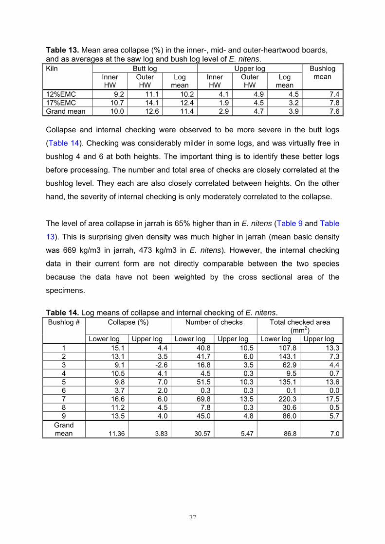
3.1.4 Collapse and internal checking – E. nitens Table 11 to Table 13 present the mean values of collapse and internal checking
measured on jarrah 400mm drying rate sample boards.
Table 11. Mean number of internal checks in the inner-, mid- and outer-heartwood boards, and as averages at the saw log and bush log level of E. nitens. Kiln Butt log Upper log Bushlog
mean Inner HW
Outer HW
Log mean
Inner HW
Outer HW
Log mean
12%EMC 26.1 23.3 24.6 7.9 3.4 5.7 14.917%EMC 43.2 29.1 36.2 6.4 4.1 5.3 20.7Grand mean 35.2 26.2 30.6 7.2 3.8 5.5 17.8 Table 12. Mean area of checks (mm2) in the inner-, mid- and outer-heartwood boards, and as averages at the saw log and bush log level of E. nitens. Kiln Butt log Upper log Bushlog
mean Inner HW
Outer HW
Log mean
Inner HW
Outer HW
Log mean
12%EMC 48.0 103.3 77.3 6.9 8.0 7.5 41.417%EMC 80.4 111.2 95.9 9.0 4.1 6.5 51.2Grand mean 65.2 107.3 86.9 8.0 6.1 7.0 46.4
37
Table 13. Mean area collapse (%) in the inner-, mid- and outer-heartwood boards, and as averages at the saw log and bush log level of E. nitens. Kiln Butt log Upper log Bushlog
mean Inner HW
Outer HW
Log mean
Inner HW
Outer HW
Log mean
12%EMC 9.2 11.1 10.2 4.1 4.9 4.5 7.417%EMC 10.7 14.1 12.4 1.9 4.5 3.2 7.8Grand mean 10.0 12.6 11.4 2.9 4.7 3.9 7.6 Collapse and internal checking were observed to be more severe in the butt logs
(Table 14). Checking was considerably milder in some logs, and was virtually free in
bushlog 4 and 6 at both heights. The important thing is to identify these better logs
before processing. The number and total area of checks are closely correlated at the
bushlog level. They each are also closely correlated between heights. On the other
hand, the severity of internal checking is only moderately correlated to the collapse.
The level of area collapse in jarrah is 65% higher than in E. nitens (Table 9 and Table
13). This is surprising given density was much higher in jarrah (mean basic density
was 669 kg/m3 in jarrah, 473 kg/m3 in E. nitens). However, the internal checking
data in their current form are not directly comparable between the two species
because the data have not been weighted by the cross sectional area of the
specimens.
Table 14. Log means of collapse and internal checking of E. nitens. Bushlog # Collapse (%) Number of checks Total checked area
(mm2) Lower log Upper log Lower log Upper log Lower log Upper log
1 15.1 4.4 40.8 10.5 107.8 13.32 13.1 3.5 41.7 6.0 143.1 7.33 9.1 -2.6 16.8 3.5 62.9 4.44 10.5 4.1 4.5 0.3 9.5 0.75 9.8 7.0 51.5 10.3 135.1 13.66 3.7 2.0 0.3 0.3 0.1 0.07 16.6 6.0 69.8 13.5 220.3 17.58 11.2 4.5 7.8 0.3 30.6 0.59 13.5 4.0 45.0 4.8 86.0 5.7
Grand mean 11.36 3.83 30.57 5.47 86.8 7.0
38
3.2 Relationships of wood properties to drying rate and drying degrade
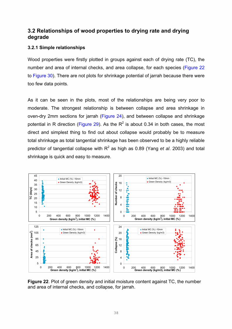
3.2.1 Simple relationships Wood properties were firstly plotted in groups against each of drying rate (TC), the
number and area of internal checks, and area collapse, for each species (Figure 22
to Figure 30). There are not plots for shrinkage potential of jarrah because there were
too few data points.
As it can be seen in the plots, most of the relationships are being very poor to
moderate. The strongest relationship is between collapse and area shrinkage in
oven-dry 2mm sections for jarrah (Figure 24), and between collapse and shrinkage
potential in R direction (Figure 29). As the R2 is about 0.34 in both cases, the most
direct and simplest thing to find out about collapse would probably be to measure
total shrinkage as total tangential shrinkage has been observed to be a highly reliable
predictor of tangential collapse with R2 as high as 0.89 (Yang et al. 2003) and total
shrinkage is quick and easy to measure.
5
10
15
20
25
30
35
40
45
0 200 400 600 800 1000 1200 1400Green density (kg/m3), initial MC (%)
TC (d
ays)
Initial MC (%) -10mm
Green Density (kg/m3)
0
4
8
12
16
20
0 200 400 600 800 1000 1200 1400Green density (kg/m3), initial MC (%)
Num
ber o
f che
cks
Initial MC (%) -10mm
Green Density (kg/m3)
5
25
45
65
85
105
125
0 200 400 600 800 1000 1200 1400Green density (kg/m3), initial MC (%)
Are
a of
che
cks
(mm
2 ) Initial MC (%) -10mm
Green Density (kg/m3)
0
4
8
12
16
20
24
0 200 400 600 800 1000 1200 1400Green density (kg/m3), initial MC (%)
Col
laps
e (%
)
Initial MC (%) -10mm
Green Density (kg/m3)
Figure 22. Plot of green density and initial moisture content against TC, the number and area of internal checks, and collapse, for jarrah.
39
5
10
15
20
25
30
35
40
45
0 1 2 3 4 5 6 7 8 9 10 11Extractive contents (%)
TC (d
ays)
Cold water (%)Hot water (%)Methanol (%)1% NaOH (%)
0
4
8
12
16
20
0 1 2 3 4 5 6 7 8 9 10 11Extractive contents (%)
Num
ber o
f che
cks
Cold water (%)Hot water (%)Methanol (%)1% NaOH (%)
5
25
45
65
85
105
125
0 1 2 3 4 5 6 7 8 9 10 11Extractive contents (%)
Are
a of
che
cks
(mm
2 )
Cold water (%)Hot water (%)Methanol (%)1% NaOH (%)
0
4
8
12
16
20
24
0 1 2 3 4 5 6 7 8 9 10 11Extractive contents (%)
Col
laps
e (%
)
Cold water (%)Hot water (%)Methanol (%)1% NaOH (%)
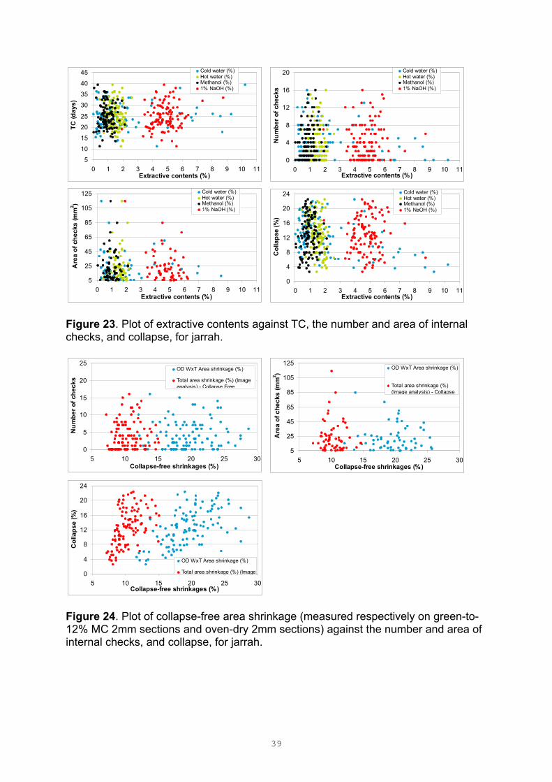
Figure 23. Plot of extractive contents against TC, the number and area of internal checks, and collapse, for jarrah.
0
5
10
15
20
25
5 10 15 20 25 30Collapse-free shrinkages (%)
Num
ber o
f che
cks
OD WxT Area shrinkage (%)
Total area shrinkage (%) (Imageanalysis) - Collapse Free
5
25
45
65
85
105
125
5 10 15 20 25 30Collapse-free shrinkages (%)
Are
a of
che
cks
(mm
2 )
OD WxT Area shrinkage (%)
Total area shrinkage (%)(Image analysis) - Collapse
0
4
8
12
16
20
24
5 10 15 20 25 30Collapse-free shrinkages (%)
Col
laps
e (%
)
OD WxT Area shrinkage (%)
Total area shrinkage (%) (Image
Figure 24. Plot of collapse-free area shrinkage (measured respectively on green-to-12% MC 2mm sections and oven-dry 2mm sections) against the number and area of internal checks, and collapse, for jarrah.

40
5
10
15
20
25
30
35
40
45
2500 3000 3500 4000 4500Acoustic velocities (m/s)
TC (d
ays)
Bushlog AcousticVelocities (m/s)Acoustic Velocities
0
4
8
12
16
20
2500 3000 3500 4000 4500Acoustic velocities (m/s)
Num
ber o
f che
cks
Bushlog AcousticVelocities (m/s)Acoustic Velocities
5
25
45
65
85
105
125
2500 3000 3500 4000 4500Acoustic velocities (m/s)
Are
a of
che
cks
(mm
2 ) Bushlog AcousticVelocities (m/s)Acoustic Velocities
0
4
8
12
16
20
24
2500 3000 3500 4000 4500Acoustic velocities (m/s)
Col
laps
e (%
)
Bushlog AcousticVelocities (m/s)Acoustic Velocities
Figure 25. Plot of bushlog and 400mm drying-rate sample board acoustic velocities against TC, the number and area of internal checks, and collapse, for jarrah.
0
5
10
15
20
25
0 200 400 600 800 1000 1200
Green density (kg/m3), Initial MC (%)
Are
a C
olla
pse
(%)
Initial MC (%) -10mmGreen Density (kg/m3)
4
6
8
10
12
14
16
18
20
0 200 400 600 800 1000 1200Green density (kg/m3), Initial MC (%)
TC (d
ays)
Initial MC (%) -10mmGreen Density (kg/m3)
0
5
10
15
20
25
0 200 400 600 800 1000 1200
Green density (kg/m3), Initial MC (%)
Num
ber o
f int
erna
l che
cks
Initial MC (%) -10mmGreen Density (kg/m3)
0
5
10
15
20
25
0 200 400 600 800 1000 1200
Green density (kg/m3), Initial MC (%)
Are
a of
inte
rnal
che
cks
(mm
2 )
Initial MC (%) -10mmGreen Density (kg/m3)
Figure 26. Plot of green density and initial moisture content against TC, the number and area of internal checks, and collapse, for E. nitens.
41
0
5
10
15
20
25
0.4 0.8 1.2 1.6 2.0 2.4 2.8 3.2 3.6 4.0
Extractive Contents (%)
Are
a C
olla
pse
(%)
Cold water (%)Hot water (%)Methanol (%)1% NaOH (%)
0
20
40
60
80
100
120
0.4 0.8 1.2 1.6 2.0 2.4 2.8 3.2 3.6 4.0
Extractive Contents (%)
Num
ber o
f Int
erna
l Che
cks Cold water (%)
Hot water (%)Methanol (%)1% NaOH (%)
0
50
100
150
200
250
300
350
400
0.4 0.8 1.2 1.6 2.0 2.4 2.8 3.2 3.6 4.0
Extractive Contents (%)
Are
a of
Inte
rnal
Che
cks
(mm
2 ) Cold water (%)Hot water (%)Methanol (%)1% NaOH (%)
4
6
8
10
12
14
16
18
20
0.4 0.8 1.2 1.6 2.0 2.4 2.8 3.2 3.6 4.0
Extractive Contents (%)
TC (d
ays)
Cold water (%)Hot water (%)Methanol (%)1% NaOH (%)
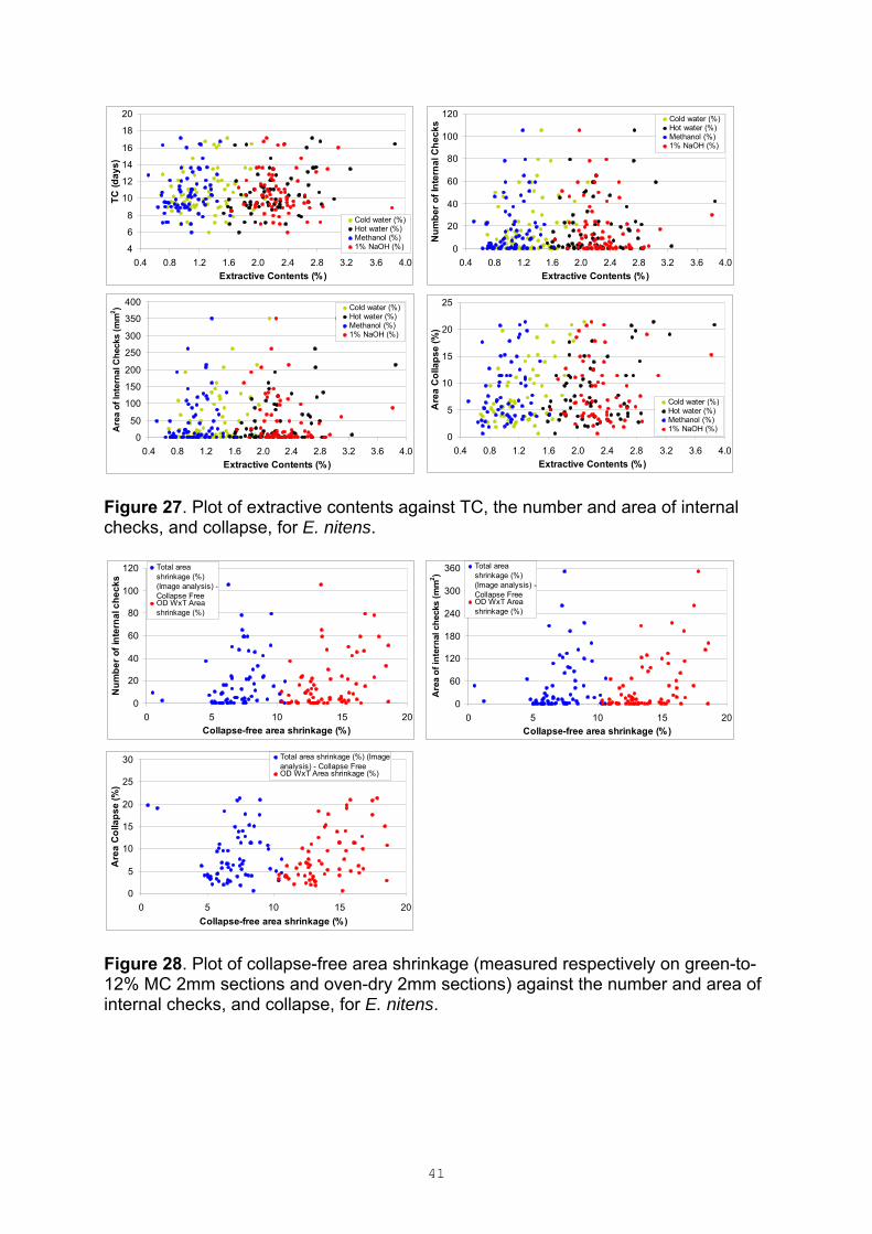
Figure 27. Plot of extractive contents against TC, the number and area of internal checks, and collapse, for E. nitens.
0
5
10
15
20
25
30
0 5 10 15 20
Collapse-free area shrinkage (%)
Are
a C
olla
pse
(%)
Total area shrinkage (%) (Imageanalysis) - Collapse FreeOD WxT Area shrinkage (%)
0
20
40
60
80
100
120
0 5 10 15 20
Collapse-free area shrinkage (%)
Num
ber o
f int
erna
l che
cks
Total areashrinkage (%)(Image analysis) -Collapse FreeOD WxT Areashrinkage (%)
0
60
120
180
240
300
360
0 5 10 15 20
Collapse-free area shrinkage (%)
Are
a of
inte
rnal
che
cks
(mm
2 )
Total areashrinkage (%)(Image analysis) -Collapse FreeOD WxT Areashrinkage (%)
Figure 28. Plot of collapse-free area shrinkage (measured respectively on green-to-12% MC 2mm sections and oven-dry 2mm sections) against the number and area of internal checks, and collapse, for E. nitens.
42
0
5
10
15
20
25
-5 0 5 10 15 20
Collapse-present shrinkage potential (%)
Are
a C
olla
pse
(%)
Shrinkage potential R (%)Shrinkage potential T (%)
0
20
40
60
80
100
120
-5 0 5 10 15 20
Collapse-present shrinkage potential (%)
Num
ber o
f int
erna
l che
cks
Shrinkage potential R (%)Shrinkage potential T (%)
0
60
120
180
240
300
360
-10 -5 0 5 10 15 20
Collapse-present shrinkage potential (%)
Are
a of
inte
rnal
che
cks
(mm
2 ) Shrinkagepotential R (%)
Shrinkagepotential T (%)
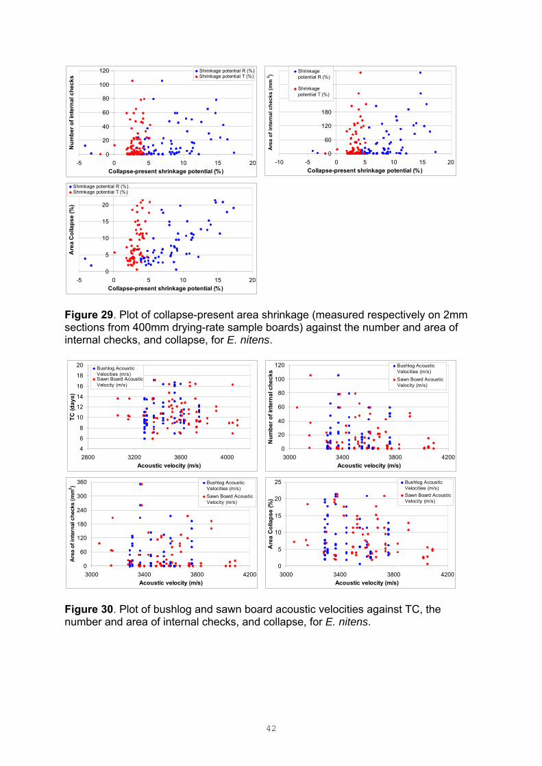
Figure 29. Plot of collapse-present area shrinkage (measured respectively on 2mm sections from 400mm drying-rate sample boards) against the number and area of internal checks, and collapse, for E. nitens.
4
6
8
10
12
14
16
18
20
2800 3200 3600 4000
Acoustic velocity (m/s)
TC (d
ays)
Bushlog AcousticVelocities (m/s)Sawn Board AcousticVelocity (m/s)
0
5
10
15
20
25
3000 3400 3800 4200
Acoustic velocity (m/s)
Are
a C
olla
pse
(%)
Bushlog AcousticVelocities (m/s)
Sawn Board AcousticVelocity (m/s)
0
20
40
60
80
100
120
3000 3400 3800 4200
Acoustic velocity (m/s)
Num
ber o
f int
erna
l che
cks
Bushlog AcousticVelocities (m/s)
Sawn Board AcousticVelocity (m/s)
0
60
120
180
240
300
360
3000 3400 3800 4200
Acoustic velocity (m/s)
Are
a of
inte
rnal
che
cks
(mm
2 ) Bushlog AcousticVelocities (m/s)
Sawn Board AcousticVelocity (m/s)
Figure 30. Plot of bushlog and sawn board acoustic velocities against TC, the number and area of internal checks, and collapse, for E. nitens.
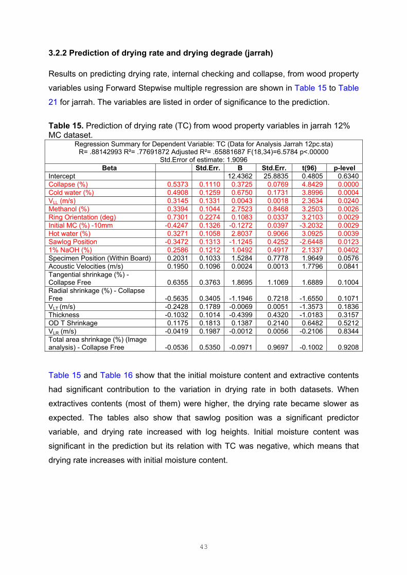
43
3.2.2 Prediction of drying rate and drying degrade (jarrah) Results on predicting drying rate, internal checking and collapse, from wood property
variables using Forward Stepwise multiple regression are shown in Table 15 to Table
21 for jarrah. The variables are listed in order of significance to the prediction.
Table 15. Prediction of drying rate (TC) from wood property variables in jarrah 12% MC dataset.
Regression Summary for Dependent Variable: TC (Data for Analysis Jarrah 12pc.sta) R= .88142993 R²= .77691872 Adjusted R²= .65881687 F(18,34)=6.5784 p<.00000
Std.Error of estimate: 1.9096 Beta Std.Err. B Std.Err. t(96) p-level
Intercept 12.4362 25.8835 0.4805 0.6340Collapse (%) 0.5373 0.1110 0.3725 0.0769 4.8429 0.0000Cold water (%) 0.4908 0.1259 0.6750 0.1731 3.8996 0.0004VLL (m/s) 0.3145 0.1331 0.0043 0.0018 2.3634 0.0240Methanol (%) 0.3394 0.1044 2.7523 0.8468 3.2503 0.0026Ring Orientation (deg) 0.7301 0.2274 0.1083 0.0337 3.2103 0.0029Initial MC (%) -10mm -0.4247 0.1326 -0.1272 0.0397 -3.2032 0.0029Hot water (%) 0.3271 0.1058 2.8037 0.9066 3.0925 0.0039Sawlog Position -0.3472 0.1313 -1.1245 0.4252 -2.6448 0.01231% NaOH (%) 0.2586 0.1212 1.0492 0.4917 2.1337 0.0402Specimen Position (Within Board) 0.2031 0.1033 1.5284 0.7778 1.9649 0.0576Acoustic Velocities (m/s) 0.1950 0.1096 0.0024 0.0013 1.7796 0.0841Tangential shrinkage (%) - Collapse Free 0.6355 0.3763 1.8695 1.1069 1.6889 0.1004Radial shrinkage (%) - Collapse Free -0.5635 0.3405 -1.1946 0.7218 -1.6550 0.1071VLT (m/s) -0.2428 0.1789 -0.0069 0.0051 -1.3573 0.1836Thickness -0.1032 0.1014 -0.4399 0.4320 -1.0183 0.3157OD T Shrinkage 0.1175 0.1813 0.1387 0.2140 0.6482 0.5212VLR (m/s) -0.0419 0.1987 -0.0012 0.0056 -0.2106 0.8344Total area shrinkage (%) (Image analysis) - Collapse Free -0.0536 0.5350 -0.0971 0.9697 -0.1002 0.9208 Table 15 and Table 16 show that the initial moisture content and extractive contents
had significant contribution to the variation in drying rate in both datasets. When
extractives contents (most of them) were higher, the drying rate became slower as
expected. The tables also show that sawlog position was a significant predictor
variable, and drying rate increased with log heights. Initial moisture content was
significant in the prediction but its relation with TC was negative, which means that
drying rate increases with initial moisture content.

44
Table 16. Prediction of drying rate (TC) from wood property variable in jarrah 17% MC dataset.
Regression Summary for Dependent Variable: TC (Data for Analysis Jarrah 17pc.sta) R= .82662555 R²= .68330980 Adjusted R²= .52948885 F(17,35)=4.4422 p<.00009
Std.Error of estimate: 3.3654 Beta Std.Err. B Std.Err. t(96) p-level
Intercept 17.9173 42.4123 0.4225 0.6753Initial MC (%) -10mm -0.5828 0.1358 -0.2547 0.0594 -4.2909 0.0001Methanol (%) -0.4167 0.1426 -4.9646 1.6987 -2.9225 0.0060Sawlog Position -0.3710 0.1271 -1.8031 0.6176 -2.9195 0.0061Acoustic Velocities (m/s) 0.3582 0.1266 0.0065 0.0023 2.8290 0.0077Hot water (%) -0.3317 0.1344 -3.8207 1.5476 -2.4688 0.0186OD T Shrinkage 0.4523 0.1847 0.8930 0.3647 2.4487 0.01951% NaOH (%) 0.2983 0.1226 1.6281 0.6692 2.4330 0.0202Total area shrinkage (%) (Image analysis) - Collapse Free
-0.3649 0.1528 -0.9476 0.3968 -2.3880 0.0225
Thickness 0.2781 0.1180 1.0648 0.4516 2.3577 0.0241Ring Orientation (deg) -0.4002 0.1776 -0.0891 0.0395 -2.2529 0.0306VLR (m/s) -0.5039 0.2364 -0.0215 0.0101 -2.1310 0.0402VLT
(m/s) -0.3801 0.2140 -0.0163 0.0092 -1.7760 0.0844Cold water (%) 0.2388 0.1436 0.5391 0.3241 1.6634 0.1052Bushlog # -0.2439 0.1619 -0.4554 0.3023 -1.5067 0.1409Green Density (kg/m3) -0.1985 0.1385 -0.0189 0.0132 -1.4333 0.1607Collapse (%) 0.1801 0.1456 0.1739 0.1406 1.2366 0.2245 VLL (m/s) 0.1511 0.1479 0.0031 0.0030 1.0216 0.3140
The contribution from other variables to TC is not straight forward to assess. In one
example, the ring orientation is moderately to highly significant but the sign of the
regression coefficients differs between the two datasets. In another example, drying
rate decreases as collapse increases in both datasets, but the contribution from
collapse is significant only in the 12% dataset. The fact that important predictor
variables vary between 12% and 17% datasets is probably at least partly due to high
levels of inter-correlation between predictor variables.
It is surprising the R2 for predicting TC was higher in 12% MC than 17% MC dataset.
The 17% MC data generally had higher TC’s and normally higher means have
greater variation that can be predicted.

45
Table 17. Prediction of the number of internal checks from wood property variables in jarrah 12% MC dataset. Regression Summary for Dependent Variable: Number of checks in range: (Data for Analysis Jarrah
12pc.sta) R= .84382738 R²= .71204464 Adjusted R²= .62565804 F(12,40)=8.2425 p<.00000 Std.Error of estimate: 2.7247
Beta Std.Err. B Std.Err. t(96) p-level
Intercept -
97.180241.0401 -2.3679 0.0228
Ring Orientation (deg) -0.8313 0.1542 -0.1679 0.0312 -5.3901 0.0000Sawlog Position 0.2875 0.0960 1.2685 0.4234 2.9958 0.0047Initial MC (%) -10mm 0.7317 0.2861 0.2986 0.1167 2.5578 0.0144Specimen Position (Within Board) -0.2294 0.0977 -2.3521 1.0018 -2.3479 0.0239Bushlog Acoustic Velocities (m/s) -0.2115 0.0933 -0.0042 0.0019 -2.2663 0.0289Radial shrinkage (%) - Collapse Free
0.3511 0.1607 1.0140 0.4640 2.1854 0.0348
VLT (m/s) 0.2026 0.1113 0.0079 0.0043 1.8201 0.0762
Basic Density (kg/m3) -10mm 0.6035 0.4023 0.0481 0.0321 1.5002 0.1414Thickness 0.1295 0.1035 0.7517 0.6010 1.2507 0.2183OD W Shrinkage 0.1208 0.1138 0.2275 0.2145 1.0608 0.2951Green Density (kg/m3) 0.0968 0.2214 0.0084 0.0191 0.4374 0.6642Collapse (%) 0.0120 0.1081 0.0113 0.1020 0.1111 0.9121 Table 18. Prediction of the number of internal checks from wood property variables in jarrah 17% MC dataset. Regression Summary for Dependent Variable: Number of checks in range: (Data for Analysis Jarrah
17pc.sta) R= .74102135 R²= .54911264 Adjusted R²= .45474087 F(9,43)=5.8186 p<.00003 Std.Error of estimate: 2.4036
Beta Std.Err. B Std.Err. t(96) p-level
Intercept -
84.278025.5084 -3.3039 0.0019
Initial MC (%) -10mm 0.7275 0.2204 0.2109 0.0639 3.3003 0.0019Ring Orientation (deg) -0.3839 0.1446 -0.0567 0.0213 -2.6554 0.0111Basic Density (kg/m3) -10mm 0.5838 0.2357 0.0332 0.0134 2.4769 0.0173Thickness 0.2799 0.1266 0.7108 0.3215 2.2110 0.0324OD W Shrinkage 0.2556 0.1322 0.3417 0.1767 1.9332 0.0598Collapse (%) 0.2579 0.1548 0.1652 0.0992 1.6658 0.1030Cold water (%) 0.2088 0.1292 0.3127 0.1935 1.6155 0.1135Specimen Position (Within Board) 0.2139 0.1352 1.6026 1.0129 1.5822 0.1209Methanol (%) 0.1353 0.1187 1.0696 0.9386 1.1397 0.2607 Table 17 And Table 18 show that the number of internal checks increased
significantly with initial moisture content and also when the growth rings became
more back-sawn oriented.
The number of internal checks increased with collapse and board thickness as well
but the contribution from these two variables was not significant. Extractive contents
were not significant predictor variables.
Again, the contribution from other variables to the number of internal checks is not
straight forward to assess, possibly due to high levels of inter-correlation between
predictor variables. In one example, the number of checks increased as basic density
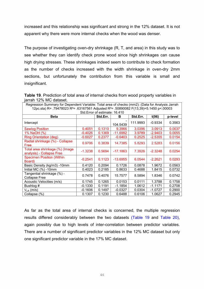
46
increased and this relationship was significant and strong in the 12% dataset. It is not
apparent why there were more internal checks when the wood was denser.
The purpose of investigating oven-dry shrinkage (R, T, and area) in this study was to
see whether they can identify check prone wood since high shrinkages can cause
high drying stresses. These shrinkages indeed seem to contribute to check formation
as the number of checks increased with the width shrinkage in oven-dry 2mm
sections, but unfortunately the contribution from this variable is small and
insignificant.
Table 19. Prediction of total area of internal checks from wood property variables in jarrah 12% MC dataset. Regression Summary for Dependent Variable: Total area of checks (mm2): (Data for Analysis Jarrah
12pc.sta) R= .79478023 R²= .63167561 Adjusted R²= .50890082 F(13,39)=5.1450 p<.00003 Std.Error of estimate: 16.410
Beta Std.Err. B Std.Err. t(96) p-level
Intercept -
104.5439111.9993 -0.9334 0.3563
Sawlog Position 0.4051 0.1310 9.3966 3.0396 3.0913 0.00371% NaOH (%) -0.4026 0.1369 -11.6992 3.9789 -2.9403 0.0055Ring Orientation (deg) -0.6027 0.2377 -0.6403 0.2525 -2.5355 0.0154Radial shrinkage (%) - Collapse Free
0.9706 0.3839 14.7385 5.8293 2.5283 0.0156
Total area shrinkage (%) (Image analysis) - Collapse Free
-1.3238 0.5694 -17.1863 7.3926 -2.3248 0.0254
Specimen Position (Within Board)
-0.2541 0.1123 -13.6955 6.0544 -2.2621 0.0293
Basic Density (kg/m3) -10mm 0.4120 0.2094 0.1726 0.0878 1.9672 0.0563Initial MC (%) -10mm 0.4023 0.2185 0.8633 0.4688 1.8415 0.0732Tangential shrinkage (%) - Collapse Free
0.7478 0.4076 15.7577 8.5894 1.8346 0.0742
Acoustic Velocities (m/s) 0.1745 0.1265 0.0153 0.0111 1.3788 0.1758Bushlog # -0.1330 0.1191 -1.1854 1.0612 -1.1171 0.2708VLR (m/s) -0.1606 0.1497 -0.0327 0.0304 -1.0727 0.2900Collapse (%) 0.1307 0.1230 0.6488 0.6106 1.0627 0.2945
As far as the total area of internal checks is concerned, the multiple regression
results differed considerably between the two datasets (Table 19 and Table 20),
again possibly due to high levels of inter-correlation between predictor variables.
There are a number of significant predictor variables in the 12% MC dataset but only
one significant predictor variable in the 17% MC dataset.

47
Table 20. Prediction of total area of internal checks from wood property variables in jarrah 17% MC dataset. Regression Summary for Dependent Variable: Total area of checks (mm2): (Data for Analysis Jarrah
17pc.sta) R= .58102903 R²= .33759473 Adjusted R²= .19895177 F(9,43)=2.4350 p<.02457 Std.Error of estimate: 9.2556
Beta Std.Err. B Std.Err. t(96) p-level
Intercept -
131.480666.9553 -1.9637 0.0561
1% NaOH (%) -0.3107 0.1306 -3.5740 1.5025 -2.3787 0.0219Initial MC (%) -10mm 0.3272 0.1633 0.3014 0.1504 2.0043 0.0514VLT
(m/s) 0.4657 0.2483 0.0420 0.0224 1.8752 0.0676Bushlog # -0.2654 0.1448 -1.0446 0.5699 -1.8328 0.0738Ring Orientation (deg) -0.2991 0.1810 -0.1403 0.0849 -1.6528 0.1057Acoustic Velocities (m/s) 0.2134 0.1434 0.0082 0.0055 1.4882 0.1440VLR (m/s) 0.3971 0.2838 0.0357 0.0255 1.3994 0.1689Green Density (kg/m3) 0.1623 0.1437 0.0325 0.0288 1.1294 0.2650Specimen Position (Within Board)
0.1386 0.1358 3.3000 3.2326 1.0209 0.3130
The extractive content at 1% NaOH extraction condition is a significantly predictor
variable in both datasets, and the total area of internal checks decreased with this
extractive content. Given this and also that extractive contents are not significant in
predicting the number of checks (Table 17 and Table 18), extractive contents in
jarrah may not have a significant role in check development in this study.
Again, the contribution from other variables to the number of internal checks is not
straight forward to assess, possibly due to high levels of inter-correlation between
predictor variables. In one example, the total area shrinkage in green-to-12% MC
2mm sections is a strong and the strongest predictor variable among all variables in
the 12% dataset but its role in check development is difficult to explain due to the
negative sign of the regression coefficient. In another example, radial shrinkage in
these sections is also a strong predictor variable in the 12% dataset (a positive
relationship) but it had no role in the prediction in the 17% dataset.
Shrinkages in oven-dry 2mm sections had too small contribution in the prediction that
they were not even entered into the regression equations.
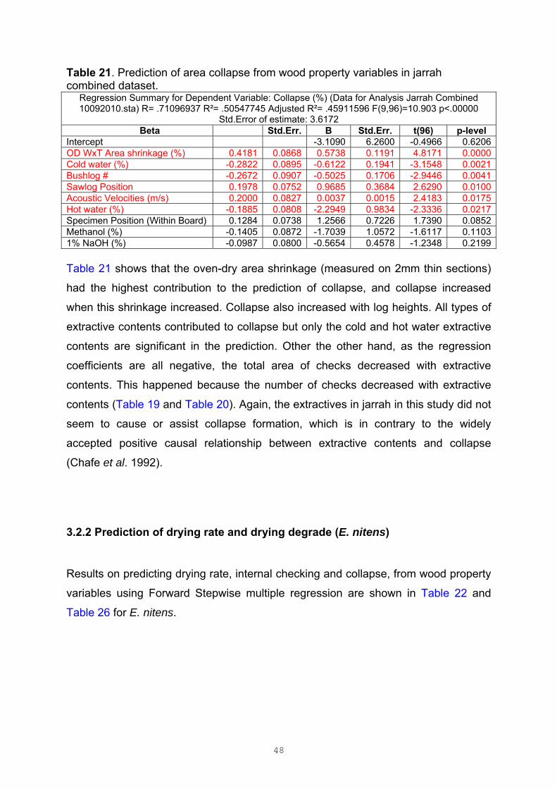
48
Table 21. Prediction of area collapse from wood property variables in jarrah combined dataset.
Regression Summary for Dependent Variable: Collapse (%) (Data for Analysis Jarrah Combined 10092010.sta) R= .71096937 R²= .50547745 Adjusted R²= .45911596 F(9,96)=10.903 p<.00000
Std.Error of estimate: 3.6172 Beta Std.Err. B Std.Err. t(96) p-level
Intercept -3.1090 6.2600 -0.4966 0.6206OD WxT Area shrinkage (%) 0.4181 0.0868 0.5738 0.1191 4.8171 0.0000Cold water (%) -0.2822 0.0895 -0.6122 0.1941 -3.1548 0.0021Bushlog # -0.2672 0.0907 -0.5025 0.1706 -2.9446 0.0041Sawlog Position 0.1978 0.0752 0.9685 0.3684 2.6290 0.0100Acoustic Velocities (m/s) 0.2000 0.0827 0.0037 0.0015 2.4183 0.0175Hot water (%) -0.1885 0.0808 -2.2949 0.9834 -2.3336 0.0217Specimen Position (Within Board) 0.1284 0.0738 1.2566 0.7226 1.7390 0.0852Methanol (%) -0.1405 0.0872 -1.7039 1.0572 -1.6117 0.11031% NaOH (%) -0.0987 0.0800 -0.5654 0.4578 -1.2348 0.2199 Table 21 shows that the oven-dry area shrinkage (measured on 2mm thin sections)
had the highest contribution to the prediction of collapse, and collapse increased
when this shrinkage increased. Collapse also increased with log heights. All types of
extractive contents contributed to collapse but only the cold and hot water extractive
contents are significant in the prediction. Other the other hand, as the regression
coefficients are all negative, the total area of checks decreased with extractive
contents. This happened because the number of checks decreased with extractive
contents (Table 19 and Table 20). Again, the extractives in jarrah in this study did not
seem to cause or assist collapse formation, which is in contrary to the widely
accepted positive causal relationship between extractive contents and collapse
(Chafe et al. 1992).
3.2.2 Prediction of drying rate and drying degrade (E. nitens)
Results on predicting drying rate, internal checking and collapse, from wood property
variables using Forward Stepwise multiple regression are shown in Table 22 and
Table 26 for E. nitens.
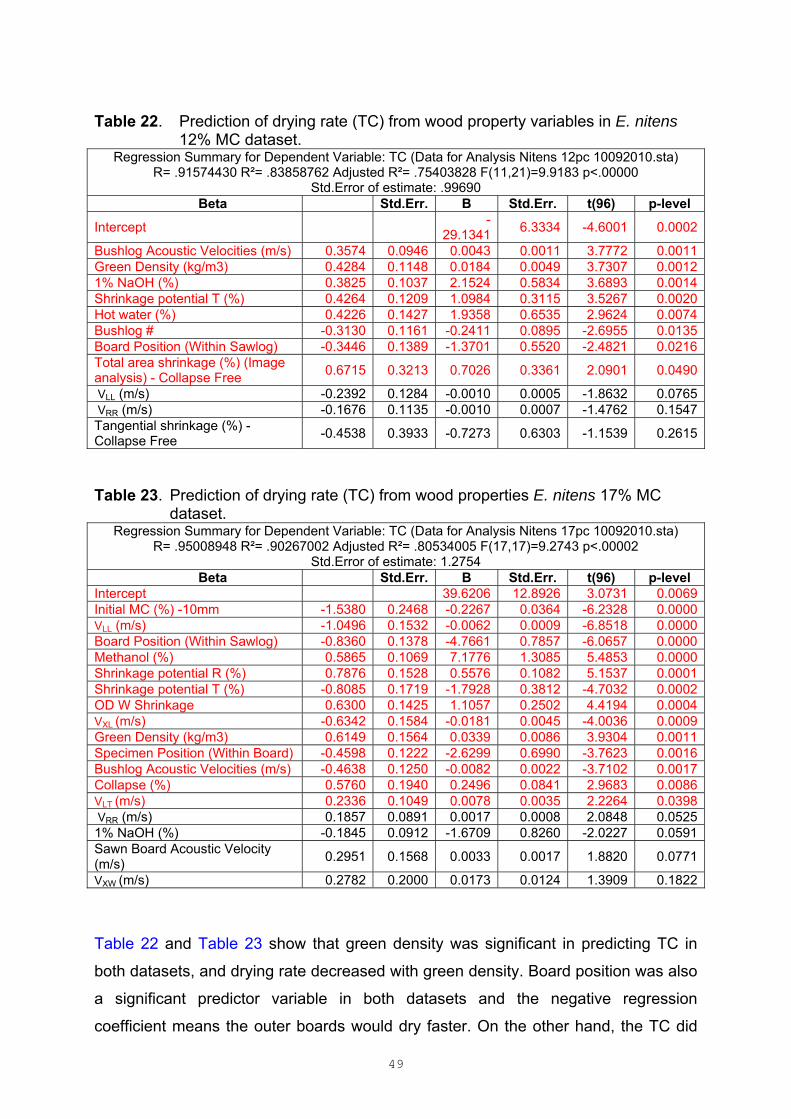
49
Table 22. Prediction of drying rate (TC) from wood property variables in E. nitens
12% MC dataset. Regression Summary for Dependent Variable: TC (Data for Analysis Nitens 12pc 10092010.sta)
R= .91574430 R²= .83858762 Adjusted R²= .75403828 F(11,21)=9.9183 p<.00000 Std.Error of estimate: .99690
Beta Std.Err. B Std.Err. t(96) p-level
Intercept -
29.13416.3334 -4.6001 0.0002
Bushlog Acoustic Velocities (m/s) 0.3574 0.0946 0.0043 0.0011 3.7772 0.0011Green Density (kg/m3) 0.4284 0.1148 0.0184 0.0049 3.7307 0.00121% NaOH (%) 0.3825 0.1037 2.1524 0.5834 3.6893 0.0014Shrinkage potential T (%) 0.4264 0.1209 1.0984 0.3115 3.5267 0.0020Hot water (%) 0.4226 0.1427 1.9358 0.6535 2.9624 0.0074Bushlog # -0.3130 0.1161 -0.2411 0.0895 -2.6955 0.0135Board Position (Within Sawlog) -0.3446 0.1389 -1.3701 0.5520 -2.4821 0.0216Total area shrinkage (%) (Image analysis) - Collapse Free
0.6715 0.3213 0.7026 0.3361 2.0901 0.0490
VLL (m/s) -0.2392 0.1284 -0.0010 0.0005 -1.8632 0.0765 VRR (m/s) -0.1676 0.1135 -0.0010 0.0007 -1.4762 0.1547Tangential shrinkage (%) - Collapse Free
-0.4538 0.3933 -0.7273 0.6303 -1.1539 0.2615
Table 23. Prediction of drying rate (TC) from wood properties E. nitens 17% MC
dataset. Regression Summary for Dependent Variable: TC (Data for Analysis Nitens 17pc 10092010.sta)
R= .95008948 R²= .90267002 Adjusted R²= .80534005 F(17,17)=9.2743 p<.00002 Std.Error of estimate: 1.2754
Beta Std.Err. B Std.Err. t(96) p-level Intercept 39.6206 12.8926 3.0731 0.0069Initial MC (%) -10mm -1.5380 0.2468 -0.2267 0.0364 -6.2328 0.0000VLL (m/s) -1.0496 0.1532 -0.0062 0.0009 -6.8518 0.0000Board Position (Within Sawlog) -0.8360 0.1378 -4.7661 0.7857 -6.0657 0.0000Methanol (%) 0.5865 0.1069 7.1776 1.3085 5.4853 0.0000Shrinkage potential R (%) 0.7876 0.1528 0.5576 0.1082 5.1537 0.0001Shrinkage potential T (%) -0.8085 0.1719 -1.7928 0.3812 -4.7032 0.0002OD W Shrinkage 0.6300 0.1425 1.1057 0.2502 4.4194 0.0004VXL
(m/s) -0.6342 0.1584 -0.0181 0.0045 -4.0036 0.0009Green Density (kg/m3) 0.6149 0.1564 0.0339 0.0086 3.9304 0.0011Specimen Position (Within Board) -0.4598 0.1222 -2.6299 0.6990 -3.7623 0.0016Bushlog Acoustic Velocities (m/s) -0.4638 0.1250 -0.0082 0.0022 -3.7102 0.0017Collapse (%) 0.5760 0.1940 0.2496 0.0841 2.9683 0.0086VLT
(m/s) 0.2336 0.1049 0.0078 0.0035 2.2264 0.0398 VRR (m/s) 0.1857 0.0891 0.0017 0.0008 2.0848 0.05251% NaOH (%) -0.1845 0.0912 -1.6709 0.8260 -2.0227 0.0591Sawn Board Acoustic Velocity (m/s)
0.2951 0.1568 0.0033 0.0017 1.8820 0.0771
VXW (m/s) 0.2782 0.2000 0.0173 0.0124 1.3909 0.1822
Table 22 and Table 23 show that green density was significant in predicting TC in
both datasets, and drying rate decreased with green density. Board position was also
a significant predictor variable in both datasets and the negative regression
coefficient means the outer boards would dry faster. On the other hand, the TC did
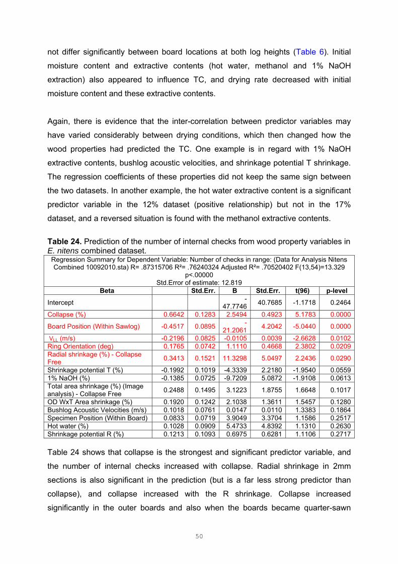
50
not differ significantly between board locations at both log heights (Table 6). Initial
moisture content and extractive contents (hot water, methanol and 1% NaOH
extraction) also appeared to influence TC, and drying rate decreased with initial
moisture content and these extractive contents.
Again, there is evidence that the inter-correlation between predictor variables may
have varied considerably between drying conditions, which then changed how the
wood properties had predicted the TC. One example is in regard with 1% NaOH
extractive contents, bushlog acoustic velocities, and shrinkage potential T shrinkage.
The regression coefficients of these properties did not keep the same sign between
the two datasets. In another example, the hot water extractive content is a significant
predictor variable in the 12% dataset (positive relationship) but not in the 17%
dataset, and a reversed situation is found with the methanol extractive contents.
Table 24. Prediction of the number of internal checks from wood property variables in E. nitens combined dataset. Regression Summary for Dependent Variable: Number of checks in range: (Data for Analysis Nitens Combined 10092010.sta) R= .87315706 R²= .76240324 Adjusted R²= .70520402 F(13,54)=13.329
p<.00000 Std.Error of estimate: 12.819
Beta Std.Err. B Std.Err. t(96) p-level
Intercept -
47.774640.7685 -1.1718 0.2464
Collapse (%) 0.6642 0.1283 2.5494 0.4923 5.1783 0.0000
Board Position (Within Sawlog) -0.4517 0.0895-
21.20614.2042 -5.0440 0.0000
VLL (m/s) -0.2196 0.0825 -0.0105 0.0039 -2.6628 0.0102Ring Orientation (deg) 0.1765 0.0742 1.1110 0.4668 2.3802 0.0209Radial shrinkage (%) - Collapse Free
0.3413 0.1521 11.3298 5.0497 2.2436 0.0290
Shrinkage potential T (%) -0.1992 0.1019 -4.3339 2.2180 -1.9540 0.05591% NaOH (%) -0.1385 0.0725 -9.7209 5.0872 -1.9108 0.0613Total area shrinkage (%) (Image analysis) - Collapse Free
0.2488 0.1495 3.1223 1.8755 1.6648 0.1017
OD WxT Area shrinkage (%) 0.1920 0.1242 2.1038 1.3611 1.5457 0.1280Bushlog Acoustic Velocities (m/s) 0.1018 0.0761 0.0147 0.0110 1.3383 0.1864Specimen Position (Within Board) 0.0833 0.0719 3.9049 3.3704 1.1586 0.2517Hot water (%) 0.1028 0.0909 5.4733 4.8392 1.1310 0.2630Shrinkage potential R (%) 0.1213 0.1093 0.6975 0.6281 1.1106 0.2717 Table 24 shows that collapse is the strongest and significant predictor variable, and
the number of internal checks increased with collapse. Radial shrinkage in 2mm
sections is also significant in the prediction (but is a far less strong predictor than
collapse), and collapse increased with the R shrinkage. Collapse increased
significantly in the outer boards and also when the boards became quarter-sawn
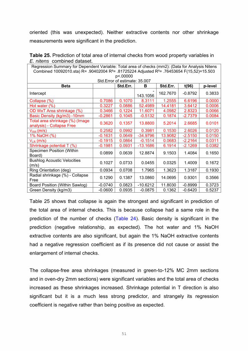
51
oriented (this was unexpected). Neither extractive contents nor other shrinkage
measurements were significant in the prediction.
Table 25. Prediction of total area of internal checks from wood property variables in E. nitens combined dataset. Regression Summary for Dependent Variable: Total area of checks (mm2): (Data for Analysis Nitens Combined 10092010.sta) R= .90402004 R²= .81725224 Adjusted R²= .76453654 F(15,52)=15.503
p<.00000 Std.Error of estimate: 35.007
Beta Std.Err. B Std.Err. t(96) p-level
Intercept -
143.1056162.7670 -0.8792 0.3833
Collapse (%) 0.7086 0.1070 8.3111 1.2555 6.6196 0.0000Hot water (%) 0.3227 0.0886 52.4989 14.4181 3.6412 0.0006OD WxT Area shrinkage (%) 0.3466 0.1224 11.6071 4.0982 2.8323 0.0066Basic Density (kg/m3) -10mm -0.2861 0.1045 -0.5132 0.1874 -2.7379 0.0084Total area shrinkage (%) (Image analysis) - Collapse Free
0.3620 0.1357 13.8800 5.2014 2.6685 0.0101
VXW (m/s) 0.2582 0.0992 0.3981 0.1530 2.6026 0.0120
1% NaOH (%) -0.1631 0.0649 -34.9796 13.9082 -2.5150 0.0150VLR (m/s) -0.1915 0.0864 -0.1514 0.0683 -2.2164 0.0311Shrinkage potential T (%) -0.1981 0.0931 -13.1686 6.1914 -2.1269 0.0382Specimen Position (Within Board)
0.0899 0.0639 12.8874 9.1503 1.4084 0.1650
Bushlog Acoustic Velocities (m/s)
0.1027 0.0733 0.0455 0.0325 1.4009 0.1672
Ring Orientation (deg) 0.0934 0.0708 1.7965 1.3623 1.3187 0.1930Radial shrinkage (%) - Collapse Free
0.1290 0.1387 13.0860 14.0695 0.9301 0.3566
Board Position (Within Sawlog) -0.0740 0.0823 -10.6212 11.8030 -0.8999 0.3723Green Density (kg/m3) -0.0600 0.0935 -0.0875 0.1362 -0.6420 0.5237 Table 25 shows that collapse is again the strongest and significant in prediction of
the total area of internal checks. This is because collapse had a same role in the
prediction of the number of checks (Table 24). Basic density is significant in the
prediction (negative relationship, as expected). The hot water and 1% NaOH
extractive contents are also significant, but again the 1% NaOH extractive contents
had a negative regression coefficient as if its presence did not cause or assist the
enlargement of internal checks.
The collapse-free area shrinkages (measured in green-to-12% MC 2mm sections
and in oven-dry 2mm sections) were significant variables and the total area of checks
increased as these shrinkages increased. Shrinkage potential in T direction is also
significant but it is a much less strong predictor, and strangely its regression
coefficient is negative rather than being positive as expected.

52
Table 26. Prediction of area collapse from wood property variables in E. nitens combined dataset.
Regression Summary for Dependent Variable: Collapse (%) (Data for Analysis Nitens Combined 10092010.sta) R= .89114985 R²= .79414805 Adjusted R²= .76623592 F(8,59)=28.452 p<.00000
Std.Error of estimate: 2.9738 Beta Std.Err. B Std.Err. t(96) p-level
Intercept 22.2342 5.8107 3.8264 0.0003Sawn Board Acoustic Velocity (m/s)
-0.3050 0.0835 -0.0074 0.0020 -3.6516 0.0006
Radial shrinkage (%) - Collapse Free
-0.2296 0.0659 -1.9861 0.5697 -3.4863 0.0009
Shrinkage potential T (%) 0.2924 0.0852 1.6578 0.4829 3.4332 0.0011Shrinkage potential R (%) 0.2814 0.0843 0.4214 0.1263 3.3365 0.0015Sawlog Position -0.1892 0.0842 -1.1555 0.5143 -2.2467 0.0284Specimen Position (Within Board) -0.1358 0.0611 -1.6595 0.7470 -2.2217 0.0302OD T Shrinkage 0.1685 0.0830 1.1677 0.5751 2.0303 0.0468OD WxT Area shrinkage (%) 0.1884 0.0956 0.5379 0.2728 1.9718 0.0533 Table 26 shows that there were no primary influencing variables for collapse
although a number of variables were significant. Collapsed decreased with the
increase of sawn board acoustic velocity (i.e. the increased of longitudinal stiffness).
Collapse increased when shrinkage potential in R and T directions increased. This is
expected because these values themselves contain a collapse component in R and
T. The T shrinkage in oven-dry 2mm sections was also significant (positive
relationship) but its contribution is relatively small.
3.3 Potential of NDE technologies in board segregation for drying rate and drying degrade
3.3.1 NIR Calibration of NIR spectra obtained from the boards surfaces shows variable
correlation with with various drying and physical properties. Table 27 shows the
results for calibration of NIR spectra with the drying time constant. In the case of
jarrah there is no correlation at all; while for shining gum there is a reasonable
correlation that exists.
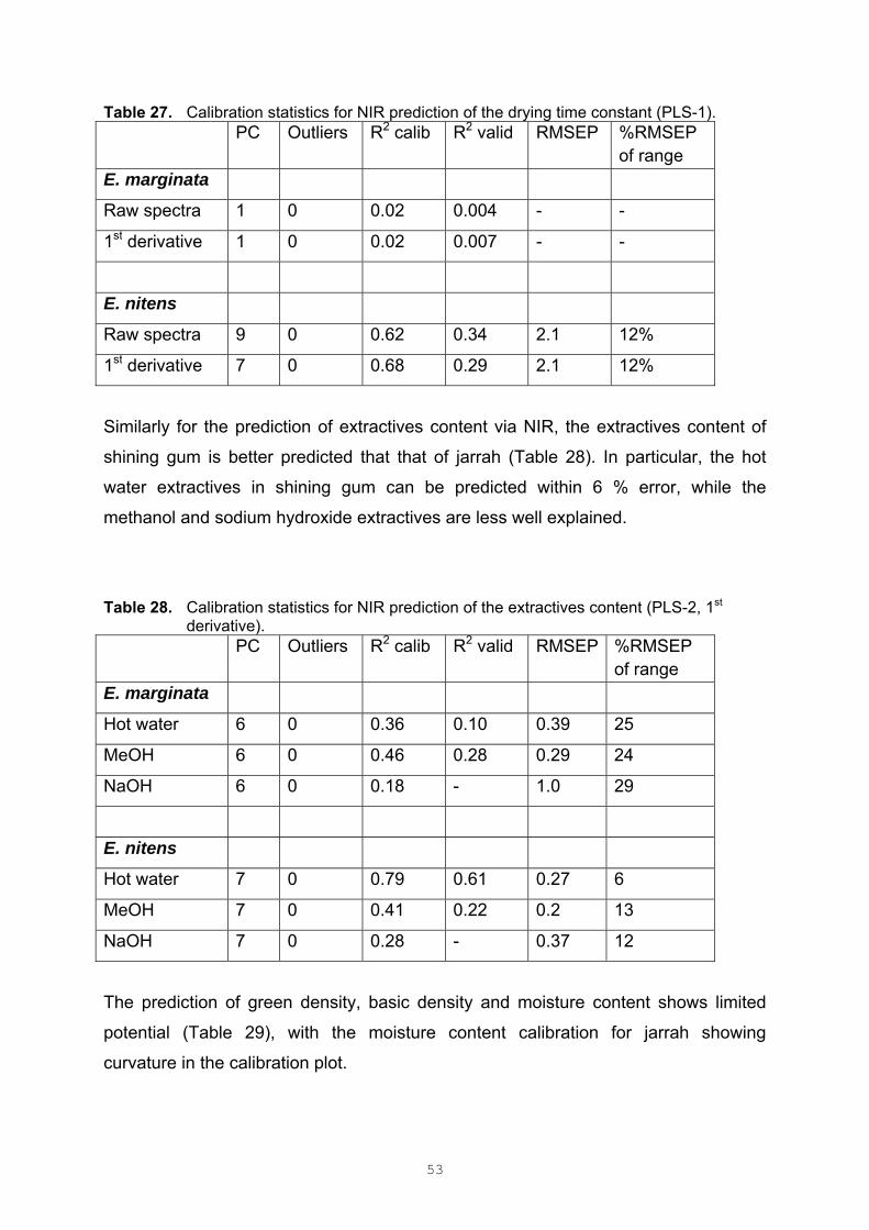
53
Table 27. Calibration statistics for NIR prediction of the drying time constant (PLS-1). PC Outliers R2 calib R2 valid RMSEP %RMSEP
of range E. marginata
Raw spectra 1 0 0.02 0.004 - -
1st derivative 1 0 0.02 0.007 - -
E. nitens
Raw spectra 9 0 0.62 0.34 2.1 12%
1st derivative 7 0 0.68 0.29 2.1 12%
Similarly for the prediction of extractives content via NIR, the extractives content of
shining gum is better predicted that that of jarrah (Table 28). In particular, the hot
water extractives in shining gum can be predicted within 6 % error, while the
methanol and sodium hydroxide extractives are less well explained.
Table 28. Calibration statistics for NIR prediction of the extractives content (PLS-2, 1st derivative).
PC Outliers R2 calib R2 valid RMSEP %RMSEP of range
E. marginata
Hot water 6 0 0.36 0.10 0.39 25
MeOH 6 0 0.46 0.28 0.29 24
NaOH 6 0 0.18 - 1.0 29
E. nitens
Hot water 7 0 0.79 0.61 0.27 6
MeOH 7 0 0.41 0.22 0.2 13
NaOH 7 0 0.28 - 0.37 12
The prediction of green density, basic density and moisture content shows limited
potential (Table 29), with the moisture content calibration for jarrah showing
curvature in the calibration plot.

54
Table 29. Calibration statistics for NIR prediction of the density and moisture content (PLS-2).
PC Outliers R2 calib R2 valid RMSEP %RMSEP
of range E. marginata
Green Density
Raw 5 0 0.56 0.48 36 17
1st derivative 8 0 0.71 0.36 41 19
2nd derivative 6 0 0.74 0.40 39 18
Basic Density
Raw 5 0 0.72 0.62 35 14
1st derivative 8 0 0.80 0.58 37 15
2nd derivative 6 0 0.78 0.52 40 16
Moisture Content
Raw 5 0 0.54 0.45 8.5 17
1st derivative 8 0 0.65 0.50 8.2 17
2nd derivative 6 0 0.62 0.36 9.3 19
E. nitens
Green Density
Raw 6 0 0.65 0.55 35 15
1st derivative 5 0 0.70 0.57 35 15
2nd derivative 4 0 0.70 0.51 37 16
Basic Density
Raw 6 0 0.62 0.53 27 15
1st derivative 5 0 0.61 0.48 28 16
2nd derivative 4 0 0.62 0.39 31 18
Moisture Content
Raw 6 0 0.81 0.73 9.5 12
1st derivative 5 0 0.78 0.73 9.6 13
2nd derivative 4 0 0.77 0.63 11 16

55
NIR was totally unable to predict the incidence of checking within either species,
which is totally consistent with results observed for P. radiate (Meder, unpublished
data). Prediction of collapse however (Table 30) showed some potential and may
offer some opportunity for screening boards that are highly prone to collapse. E.
marginata consistently showed lower error values and fewer outliers than E. nitens.
Table 30. Calibration statistics for NIR prediction of collapse (PLS-1). PC Outliers R2 calib R2 valid RMSEP %RMSEP
of range E. marginata
Raw 6 0 0.49 0.37 3.9 14
1st derivative 6 0 0.62 0.37 4.0 14
2nd derivative 4 0 0.72 0.30 4.1 15
E. nitens
Raw 6 0 - - - -
1st derivative 6 4 0.87 0.30 4.6 19
2nd derivative 4 6 0.81 0.34 4.4 18
The prediction of radial and tangential shrinkage (Table 31) was consistent with that
observed for P. radiata (Meder, unpublished data). Neither radial nor tangential
shrinkage is predicted as well as longitudinal shrinkage (not determined in this
study), but once again NIR may offer a rapid screen for boards that are highly prone
to shrinkage.
Overall the use of NIR offers some potential as a screening tool for several
properties, which taken in isolation are not worthy of further investigation, but
collectively may offer a tool to identify the worst behaving boards that could be
segregated for milder treatment.

56
Table 31. Calibration statistics for NIR prediction of radial and tangential shrinkage (PLS-2).
PC Outliers R2 calib R2 valid RMSEP %RMSEP of range
E. marginata
Raw
Radial 9 0 0.44 0.21 1.3 18
Tangential 9 0 0.37 0.13 1.2 17
1st derivative
Radial 5 0 0.38 0.20 1.3 18
Tangential 5 0 0.40 0.13 1.2 17
E. nitens
Raw
Radial 8 2 0.68 0.49 2.6 15
Tangential 8 2 0.48 0.29 0.76 14
1st derivative
Radial 5 2 0.67 0.50 2.5 15
Tangential 5 2 0.48 0.30 0.75 14
3.3.2 Acoustic and ultrasonic velocities Forward Stepwise regression was attempted to see which acoustic and ultrasonic
velocities provides the best combined predictor of drying rate (Time Constant) and
drying degrade. Only acoustic and ultrasonic velocities and specimen location data
(bushlog number, saw log position, board position and specimen position) were
included in the regression. The results are presented in Table 32 to Table 38 for
jarrah and in Table 39 to Table 43 for E. nitens.
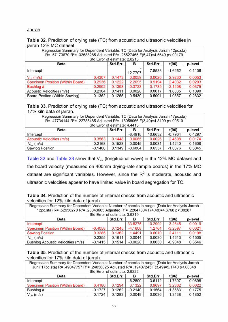
57
Jarrah Table 32. Prediction of drying rate (TC) from acoustic and ultrasonic velocities in jarrah 12% MC dataset.
Regression Summary for Dependent Variable: TC (Data for Analysis Jarrah 12pc.sta) R= .57173670 R²= .32688285 Adjusted R²= .25527465 F(5,47)=4.5649 p<.00179
Std.Error of estimate: 2.8213 Beta Std.Err. B Std.Err. t(96) p-level
Intercept -
12.77077.8533 -1.6262 0.1106
VLL (m/s) 0.4307 0.1473 0.0059 0.0020 2.9230 0.0053Specimen Position (Within Board) 0.2936 0.1222 2.2095 0.9194 2.4032 0.0203Bushlog # -0.2992 0.1398 -0.3723 0.1739 -2.1408 0.0375Acoustic Velocities (m/s) 0.2304 0.1411 0.0028 0.0017 1.6335 0.1090Board Positon (Within Sawlog) 0.1362 0.1255 0.5430 0.5001 1.0857 0.2832 Table 33. Prediction of drying rate (TC) from acoustic and ultrasonic velocities for 17% kiln data of jarrah.
Regression Summary for Dependent Variable: TC (Data for Analysis Jarrah 17pc.sta) R= .47734144 R²= .22785485 Adjusted R²= .18058066 F(3,49)=4.8199 p<.00510
Std.Error of estimate: 4.4413 Beta Std.Err. B Std.Err. t(96) p-level
Intercept -8.4918 10.6632 -0.7964 0.4297Acoustic Velocities (m/s) 0.3563 0.1448 0.0065 0.0026 2.4608 0.0174 VLL (m/s) 0.2168 0.1523 0.0045 0.0031 1.4240 0.1608Sawlog Position -0.1400 0.1349 -0.6804 0.6557 -1.0376 0.3045 Table 32 and Table 33 show that VLL (longitudinal wave) in the 12% MC dataset and
the board velocity (measured on 400mm drying-rate sample boards) in the 17% MC
dataset are significant variables. However, since the R2 is moderate, acoustic and
ultrasonic velocities appear to have limited value in board segregation for TC.
Table 34. Prediction of the number of internal checks from acoustic and ultrasonic velocities for 12% kiln data of jarrah. Regression Summary for Dependent Variable: Number of checks in range: (Data for Analysis Jarrah
12pc.sta) R= .52956270 R²= .28043665 Adjusted R²= .22047304 F(4,48)=4.6768 p<.00287 Std.Error of estimate: 3.9319
Beta Std.Err. B Std.Err. t(96) p-level Intercept 33.8275 10.2992 3.2845 0.0019Specimen Position (Within Board) -0.4058 0.1245 -4.1608 1.2764 -3.2597 0.0021Sawlog Position 0.3285 0.1362 1.4491 0.6010 2.4111 0.0198 VLL (m/s) -0.2355 0.1611 -0.0044 0.0030 -1.4613 0.1505Bushlog Acoustic Velocities (m/s) -0.1415 0.1514 -0.0028 0.0030 -0.9348 0.3546 Table 35. Prediction of the number of internal checks from acoustic and ultrasonic velocities for 17% kiln data of jarrah. Regression Summary for Dependent Variable: Number of checks in range: (Data for Analysis Jarrah
Junli 17pc.sta) R= .49047757 R²= .24056825 Adjusted R²= .19407243 F(3,49)=5.1740 p<.00348 Std.Error of estimate: 2.9222
Beta Std.Err. B Std.Err. t(96) p-level Intercept -6.2500 3.6112 -1.7307 0.0898Specimen Position (Within Board) 0.4180 0.1294 3.1322 0.9697 3.2302 0.0022Bushlog # -0.1727 0.1262 -0.2140 0.1564 -1.3683 0.1775VLR (m/s) 0.1724 0.1283 0.0049 0.0036 1.3438 0.1852
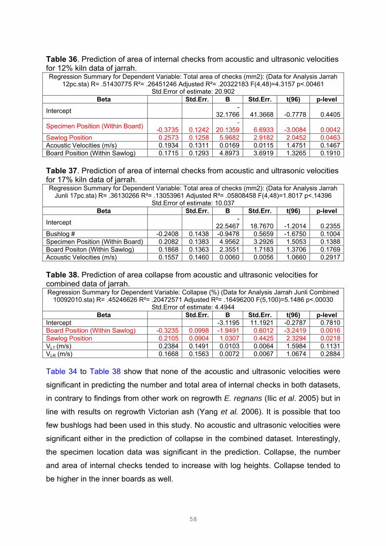
58
Table 36. Prediction of area of internal checks from acoustic and ultrasonic velocities for 12% kiln data of jarrah. Regression Summary for Dependent Variable: Total area of checks (mm2): (Data for Analysis Jarrah
12pc.sta) R= .51430775 R²= .26451246 Adjusted R²= .20322183 F(4,48)=4.3157 p<.00461 Std.Error of estimate: 20.902
Beta Std.Err. B Std.Err. t(96) p-level
Intercept
-32.1766 41.3668 -0.7778 0.4405
Specimen Position (Within Board) -0.3735 0.1242
-20.1359 6.6933 -3.0084 0.0042
Sawlog Position 0.2573 0.1258 5.9682 2.9182 2.0452 0.0463Acoustic Velocities (m/s) 0.1934 0.1311 0.0169 0.0115 1.4751 0.1467Board Position (Within Sawlog) 0.1715 0.1293 4.8973 3.6919 1.3265 0.1910 Table 37. Prediction of area of internal checks from acoustic and ultrasonic velocities for 17% kiln data of jarrah. Regression Summary for Dependent Variable: Total area of checks (mm2): (Data for Analysis Jarrah
Junli 17pc.sta) R= .36130266 R²= .13053961 Adjusted R²= .05808458 F(4,48)=1.8017 p<.14396 Std.Error of estimate: 10.037
Beta Std.Err. B Std.Err. t(96) p-level
Intercept
-22.5467 18.7670 -1.2014 0.2355
Bushlog # -0.2408 0.1438 -0.9478 0.5659 -1.6750 0.1004Specimen Position (Within Board) 0.2082 0.1383 4.9562 3.2926 1.5053 0.1388Board Positon (Within Sawlog) 0.1868 0.1363 2.3551 1.7183 1.3706 0.1769Acoustic Velocities (m/s) 0.1557 0.1460 0.0060 0.0056 1.0660 0.2917 Table 38. Prediction of area collapse from acoustic and ultrasonic velocities for combined data of jarrah. Regression Summary for Dependent Variable: Collapse (%) (Data for Analysis Jarrah Junli Combined
10092010.sta) R= .45246626 R²= .20472571 Adjusted R²= .16496200 F(5,100)=5.1486 p<.00030 Std.Error of estimate: 4.4944
Beta Std.Err. B Std.Err. t(96) p-level Intercept -3.1195 11.1921 -0.2787 0.7810Board Position (Within Sawlog) -0.3235 0.0998 -1.9491 0.6012 -3.2419 0.0016Sawlog Position 0.2105 0.0904 1.0307 0.4425 2.3294 0.0218VLT (m/s) 0.2384 0.1491 0.0103 0.0064 1.5984 0.1131VLR (m/s) 0.1668 0.1563 0.0072 0.0067 1.0674 0.2884 Table 34 to Table 38 show that none of the acoustic and ultrasonic velocities were
significant in predicting the number and total area of internal checks in both datasets,
in contrary to findings from other work on regrowth E. regnans (Ilic et al. 2005) but in
line with results on regrowth Victorian ash (Yang et al. 2006). It is possible that too
few bushlogs had been used in this study. No acoustic and ultrasonic velocities were
significant either in the prediction of collapse in the combined dataset. Interestingly,
the specimen location data was significant in the prediction. Collapse, the number
and area of internal checks tended to increase with log heights. Collapse tended to
be higher in the inner boards as well.

59
E. nitens Table 39. Prediction of drying rate (TC) from acoustic and ultrasonic velocities for 12% kiln data of E. nitens.
Regression Summary for Dependent Variable: TC (Data for Analysis Nitens 12pc 10092010.sta) R= .60055369 R²= .36066474 Adjusted R²= .29879359 F(3,31)=5.8293 p<.00280
Std.Error of estimate: 1.6340 Beta Std.Err. B Std.Err. t(96) p-level
Intercept 0.5149 6.2474 0.0824 0.9348Sawlog Position -0.5932 0.1521 -1.1413 0.2926 -3.9006 0.0005Bushlog Acoustic Velocities (m/s) 0.2237 0.1439 0.0027 0.0017 1.5547 0.1302VLL (m/s) 0.1622 0.1523 0.0006 0.0006 1.0651 0.2951 Table 40. Prediction of drying rate (TC) from acoustic and ultrasonic velocities for 17% kiln data of E. nitens.
Regression Summary for Dependent Variable: TC (Data for Analysis Nitens 17pc 10092010.sta) R= .51581859 R²= .26606882 Adjusted R²= .22019812 F(2,32)=5.8004 p<.00709
Std.Error of estimate: 2.5528 Beta Std.Err. B Std.Err. t(96) p-level
Intercept 4.6749 9.3782 0.4985 0.6215Sawlog Position -0.4970 0.1515 -1.4166 0.4319 -3.2798 0.0025Bushlog Acoustic Velocities (m/s) 0.1557 0.1515 0.0028 0.0027 1.0277 0.3118 Table 39 and Table 40 show that none of the acoustic and ultrasonic velocities were
significant variables in both datasets. Instead, sawlog position is the only significant
predictor variable, and the drying rate increased with log heights. The R2 is moderate.
Table 41. Prediction of the number of internal checks from acoustic and ultrasonic velocities for combined data of E. nitens. Regression Summary for Dependent Variable: Number of checks in range: (Data for Analysis Nitens
Combined 10092010.sta) R= .57488163 R²= .33048888 Adjusted R²= .28864444 F(4,64)=7.8980 p<.00003
Std.Error of estimate: 19.789 Beta Std.Err. B Std.Err. t(96) p-level
Intercept 48.5383 28.5661 1.6992 0.0941
Sawlog Position -0.5996 0.1142
-13.9673 2.6612 -5.2485 0.0000
VXW (m/s) 0.2068 0.1350 0.1043 0.0681 1.5320 0.1305VLR (m/s) -0.1454 0.1212 -0.0376 0.0313 -1.1993 0.2348Board Position (Within Sawlog) -0.1003 0.1056 -4.6767 4.9258 -0.9494 0.3460 Table 42. Prediction of area of internal checks from acoustic and ultrasonic velocities for combined data of E. nitens. Regression Summary for Dependent Variable: Total area of checks (mm2): (Data for Analysis Nitens
Combined 10092010.sta) R= .62775640 R²= .39407809 Adjusted R²= .34598905 F(5,63)=8.1948 p<.00001
Std.Error of estimate: 58.104 Beta Std.Err. B Std.Err. t(96) p-level
Intercept 76.2966 85.2159 0.8953 0.3740
Sawlog Position -0.6791 0.1130
-48.4390 8.0577 -6.0115 0.0000
VLR (m/s) -0.3170 0.1387 -0.2508 0.1097 -2.2862 0.0256VXW (m/s) 0.2398 0.1296 0.3702 0.2001 1.8499 0.0690Board Position (Within Sawlog) 0.1752 0.1016 25.0229 14.5001 1.7257 0.0893VLT (m/s) 0.2162 0.1270 0.1783 0.1047 1.7026 0.0936
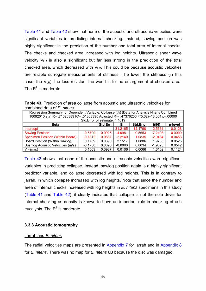
60
Table 41 and Table 42 show that none of the acoustic and ultrasonic velocities were
significant variables in predicting internal checking. Instead, sawlog position was
highly significant in the prediction of the number and total area of internal checks.
The checks and checked area increased with log heights. Ultrasonic shear wave
velocity VLR is also a significant but far less strong in the prediction of the total
checked area, which decreased with VLR. This could be because acoustic velocities
are reliable surrogate measurements of stiffness. The lower the stiffness (in this
case, the VLR), the less resistant the wood is to the enlargement of checked area.
The R2 is moderate.
Table 43. Prediction of area collapse from acoustic and ultrasonic velocities for combined data of E. nitens.
Regression Summary for Dependent Variable: Collapse (%) (Data for Analysis Nitens Combined 10092010.sta) R= .71626389 R²= .51303395 Adjusted R²= .47376250 F(5,62)=13.064 p<.00000
Std.Error of estimate: 4.4619 Beta Std.Err. B Std.Err. t(96) p-level
Intercept 31.2165 12.1790 2.5631 0.0128Sawlog Position -0.6709 0.0925 -4.0981 0.5653 -7.2498 0.0000Specimen Position (Within Board) -0.1812 0.0887 -2.2140 1.0835 -2.0434 0.0453Board Position (Within Sawlog) 0.1759 0.0890 2.1517 1.0886 1.9765 0.0525Bushlog Acoustic Velocities (m/s) -0.1758 0.0896 -0.0066 0.0034 -1.9625 0.0542VLT (m/s) 0.1509 0.0937 0.0106 0.0066 1.6102 0.1124 Table 43 shows that none of the acoustic and ultrasonic velocities were significant
variables in predicting collapse. Instead, sawlog position again is a highly significant
predictor variable, and collapse decreased with log heights. This is in contrary to
jarrah, in which collapse increased with log heights. Note that since the number and
area of internal checks increased with log heights in E. nitens specimens in this study
(Table 41 and Table 42), it clearly indicates that collapse is not the sole driver for
internal checking as density is known to have an important role in checking of ash
eucalypts. The R2 is moderate.
3.3.3 Acoustic tomography Jarrah and E. nitens The radial velocities maps are presented in Appendix 7 for jarrah and in Appendix 8
for E. nitens. There was no map for E. nitens 6B because the disc was damaged.
61
The acoustic tomograph is a map of estimated radial velocities across the disc.
These radial velocity maps were not intended to reveal or predict drying rate or
drying quality in this study for two reasons. Firstly, our FAKOPP 2D instrument only
has a single inbuilt calibration for ‘Eucalyptus’ species, which may have been based
on limited data, but it does not a specific calibration for jarrah species. The radial
velocity maps generated with the ‘Eucalyptus’ calibration will not be accurate for
jarrah. Secondly, little is known about the effect of radial stiffness on shrinkage,
collapse and internal checking. Hence, even if we had sufficiently accurate radial
velocity maps for jarrah, the maps themselves do not contain direct information on
shrinkage, collapse and internal checking. Nevertheless, we still can compare the
maps with the measured shrinkage data and see if we can observe something, and
this is what was done in this study.
Also, the maps can provide us an approximate idea on the uniformity of radial
velocities across the discs. Given the discs were all green and the effect of moisture
content was small, the radial velocities is expected to increase with density and
decrease with grain angle, in similar manner as velocities along the grain. If
concentricity and small across-log variation in radial velocity are preferred, then the
better jarrah discs would be 2, 6 and 8, and the worst jarrah discs would be 4 and 7.
Similarly, 1 and 8 would be the better E. nitens bushlogs. It is also observed for E.
nitens that (1) some bushlogs had distinct inner lower-velocity zones (e.g. bushlog 8)
whereas others did not (e.g. bushlog 7); (2) the maps turned the other way around at
the 12.5m height for most bushlogs by the outer wood zone having lower velocities.
It is expected that radial velocity maps would vary with tree height due to wood
property variation, but this cannot be ascertained for the jarrah logs since we had
only one disc from each jarrah bushlog. For E. nitens however, three discs were
obtained from each bushlog, and the overall trend is that, with increasing height, the
discs became more uniform and the outer wood tended to have lower velocities.
Based on the exiting radial velocity maps, there was no strong evidence that the
maps are capable of identifying better or worse logs in terms of drying degrade.
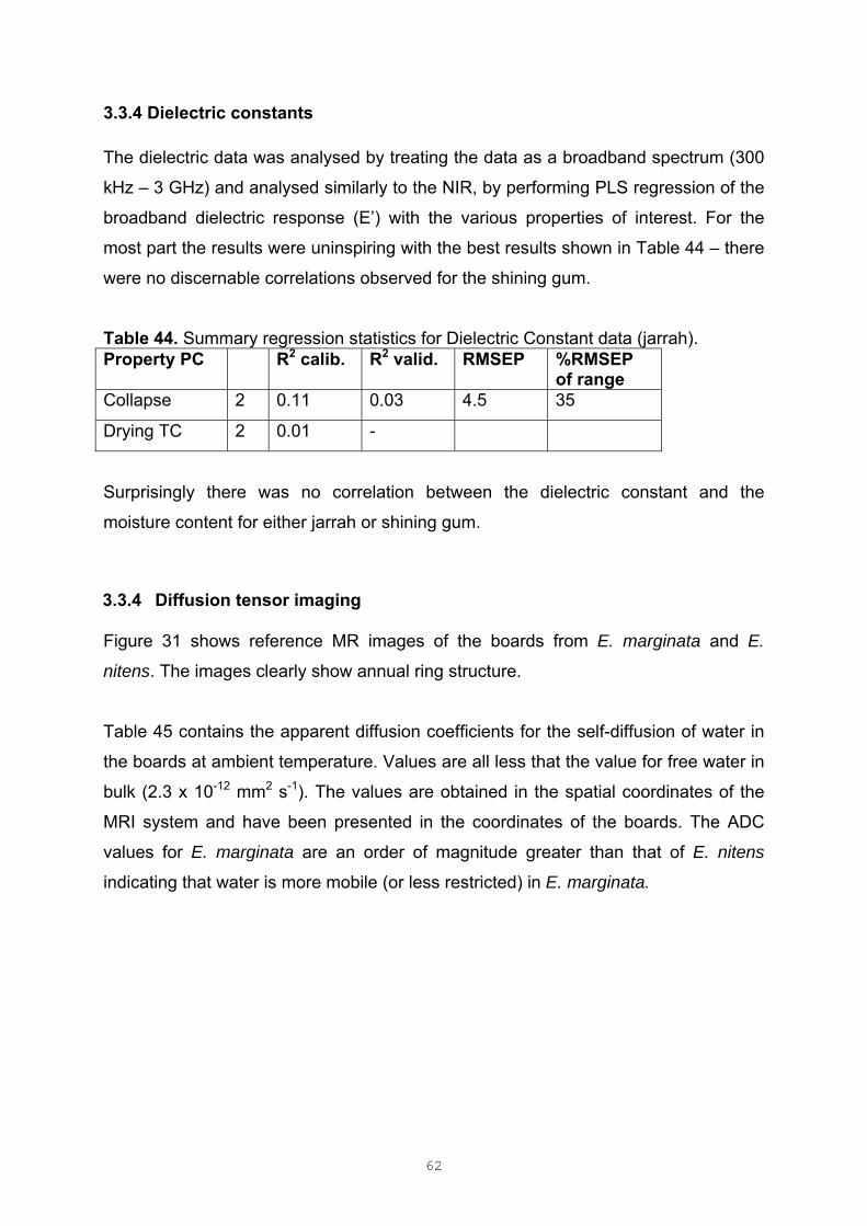
62
3.3.4 Dielectric constants The dielectric data was analysed by treating the data as a broadband spectrum (300
kHz – 3 GHz) and analysed similarly to the NIR, by performing PLS regression of the
broadband dielectric response (E’) with the various properties of interest. For the
most part the results were uninspiring with the best results shown in Table 44 – there
were no discernable correlations observed for the shining gum.
Table 44. Summary regression statistics for Dielectric Constant data (jarrah). Property PC R2 calib. R2 valid. RMSEP %RMSEP
of range Collapse 2 0.11 0.03 4.5 35
Drying TC 2 0.01 -
Surprisingly there was no correlation between the dielectric constant and the
moisture content for either jarrah or shining gum.
3.3.4 Diffusion tensor imaging Figure 31 shows reference MR images of the boards from E. marginata and E.
nitens. The images clearly show annual ring structure.
Table 45 contains the apparent diffusion coefficients for the self-diffusion of water in
the boards at ambient temperature. Values are all less that the value for free water in
bulk (2.3 x 10⁻¹² mm2 s-1). The values are obtained in the spatial coordinates of the
MRI system and have been presented in the coordinates of the boards. The ADC
values for E. marginata are an order of magnitude greater than that of E. nitens
indicating that water is more mobile (or less restricted) in E. marginata.

63
Figure 31. Localiser images (2D_Gradient Echo, TE/TR 3.7/7.8 ms, Slice 6 mm) Top to bottom: 2511, 2512, 2631, 2632; 1311, 1313, 1731, 1733; 1331,
1333, 1711, 1713.
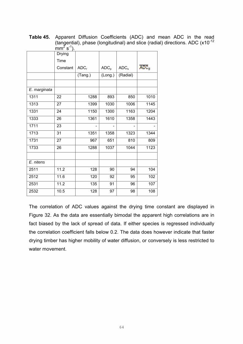
64
Table 45. Apparent Diffusion Coefficients (ADC) and mean ADC in the read (tangential), phase (longitudinal) and slice (radial) directions. ADC (x10-12 mm2 s-1).
Drying
Time
Constant ADCr ADCp ADCs �
(Tang.) (Long.) (Radial)
E. marginata
1311 22 1288 893 850 1010
1313 27 1399 1030 1006 1145
1331 24 1150 1300 1163 1204
1333 26 1361 1610 1358 1443
1711 23 - - - -
1713 31 1351 1358 1323 1344
1731 27 967 651 810 809
1733 26 1288 1037 1044 1123
E. nitens
2511 11.2 128 90 94 104
2512 11.6 120 92 95 102
2531 11.2 135 91 96 107
2532 10.5 128 97 98 108
The correlation of ADC values against the drying time constant are displayed in
Figure 32. As the data are essentially bimodal the apparent high correlations are in
fact biased by the lack of spread of data. If either species is regressed individually
the correlation coefficient falls below 0.2. The data does however indicate that faster
drying timber has higher mobility of water diffusion, or conversely is less restricted to
water movement.
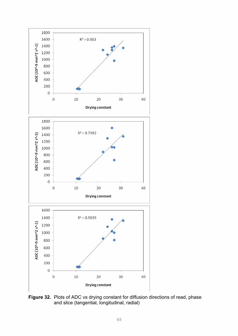
65
Figure 32. Plots of ADC vs drying constant for diffusion directions of read, phase and slice (tangential, longitudinal, radial)
66
4. Conclusions Major conclusions from the results of this study are:
No single wood property or the acoustic and ultrasonic variable was closely
correlated with drying rate, the number and area of internal checks, or collapse.
This means that none of these properties alone had sufficient potential to reliably
predict drying rate and drying degrade.
The adjusted multiple regression R2 (wood properties as predictor variables)
ranged from 0.19 to 0.80. Several or a number of wood properties are needed to
achieve this level of prediction. Whilst high R2 values are encouraging, it may not
be feasible in practice to sort or identify wood materials (at log or board levels) for
drying rate and drying degrade by measuring these significant wood properties.
Multiple regression results differed considerably between the 12% MC and 17%
MC datasets in several occasions. The results hence are not straight forward to
interpret. The fact that important predictor variables vary between the two
datasets is probably at least partly due to high levels of inter-correlation between
predictor variables. Also drying conditions themselves may also have had some
influence on the inter-correlation between predictor variables, and between
predictor and dependent variables. These might then have changed the prediction
results.
For drying rate (TC) of jarrah, the extractive contents and sawlog position were
significant variables that account for the variation of drying rate in the presence of
other variables. Drying rate decreased with most of the extractive contents but
increased with log heights. Initial moisture content was also significant in the
prediction but its relation with TC was negative, which means that drying rate
increases with initial moisture content, and this is puzzling.
Drying rate of E. nitens definitely varied with green density. It decreased with the
increase of green density. The initial moisture content and extractive contents (hot
water, methanol and 1% NaOH extraction) also appeared to account for the

67
variation of drying rate among other variables. Drying rate decreased with the
increase of initial moisture content and these extractive contents.
The number of internal checks in jarrah varied highly with initial moisture content
and ring orientation. The number of checks increased when initial moisture
content increased and the boards became more back-sawn oriented. It also
appeared to increase with collapse and board thickness to a small extent.
The number of internal checks in E. nitens varied highly with collapse. It
increased when collapsed increased. The number of checks also increased in
outer sawn boards and when shrinkage in radial direction increased.
The total area of internal checks in jarrah varied highly with collapse-free area
shrinkage in the 12% MC dataset.
The total area of internal checks of E. nitens varied highly with collapse, and
moderately with quite a few other variables. It increased with the increase of
collapse, the decrease of basic density, the increase of hot water extractives, and
the increase of area shrinkages (green-to-12% MC and green-to-oven-dry).
Interestingly, it also increased with the decrease of extractive contents from 1%
NaOH extraction, as in jarrah.
Collapse in jarrah varied with oven-dry area shrinkage, extractive contents (cold
and hot water extraction), and sawlog position. It increased with the increase of
oven-dry area shrinkage and log heights, but decreased with the increase if the
extractive contents.
Collapse in E. nitens varied primarily with several shrinkages. It increased with
the increase of shrinkage potential in R and T directions, and with the R and T
shrinkages in green-to-12% MC and green-to-oven-dry specimens, respectively.
The along-grain acoustic and ultrasonic velocity appeared to provide some level
of prediction to drying rate of only jarrah. But the R2 is moderate.

68
None of the acoustic and ultrasonic velocities, alone or combined (without wood
property variables in the regression), were significant in the prediction of drying
degrade and collapse for both species.
Log height was a consistently “influencing” variable in E. nitens. Drying rate
increased, but drying degrade and collapse decreased, in upper logs. From the
drying rate and drying degrade point of view, upper logs had better quality.
Log height was also related to the dependent variables in certain way in jarrah
although not as strong as in E. nitens. With the increase of log heights, both
drying degrade and collapse increased.
The dielectric constant was unable to be correlated with any property for either
species.
Near infrared spectroscopy showed moderate correlations for several properties,
many of which can currently only measured be measured destructively and with
great difficulty. While individually these properties are of limited interest,
collectively they may be able to identify the worst performing boards in order to
segregate them for alternate processing (e.g. milder drying conditions).
5. Recommendations It is worth considering sorting E. nitens logs by heights for drying rate and drying
degrade in both species. Further study would be required to confirm the effect of
log heights and evaluate the economical benefit.
Total shrinkage (normal shrinkage plus collapse) is a quick, simple and reliable
surrogate measurement for collapse (at least for tangential direction). For quick,
low-cost and reliable estimation of collapse, total shrinkage should be a highly
worthwhile alternative.
6. References

69
Booker, R.E. (1990) Changes in transverse wood permeability during the drying of Dacrydium cupressinum and Pinus radiata. N. Z. J. For. Sci., 20, 231-244.
Chafe, S.C. (1987) Collapse, volumetric shrinkage, specific gravity and extractives in Eucalyptus and other species. Part 2: The influence of extractives. Wood Sci. Technol. 21:27-41
Chafe, S.C. (1990) Changes in shrinkages and collapse in the wood of Eucalyptus regnans F. Muell following extraction. Holzforschung 44(4):235-244
Chafe, S.C., Barnacle, J.E., Hunter, A.J., Ilic, J., Northway, R.L. and Roza, A.N. (1992) Collapse: An introduction. CSIRO Forestry and Forest Products.
Hillis, W.E. (1962) The distribution and formation of polyphenols within the tree. In: Wood extractives and their significance wood the pulp and paper industries. New York (Hillis, W.E. ed.). Academic Press
Hoffmeyer, P., Pedersen, J. (1995) Evaluation of density and strength of Norway spruce wood by near infrared spectroscopy. Holz Roh Werkst. 53:165-170.
Ilic, J. (1999) Influence of prefreezing on shrinkage related degrade in Eucalyptus regnans F. Muell. Holz Roh Werkst. 57: 241-245.
Ilic, J. (1999) Shrinkage related degrade and its association with some physical properties in Eucalyptus regnans F. Muell. Wood Sci. Technol. 33: 425-437
Ilic, J., Bennett, P.J. (2000) Sorting eucalypt logs and boards to facilitate drying. Proc. IUFRO, The Future of Eucalypts for Wood Products, Tasmania, Australia.
Ilic, J. (2001) Variation of dynamic elastic modulus and wave velocity in the fibre direction with other properties during drying. Wood Sci. Technol. 35:157-166.
Ilic, J., Northway, R., Thumm, A., Wright, J. (2005) The development of NDE technologies for use in the hardwood sawmilling industry. FWPRDC report PN03.1317.
Keey, R.B., Langrish, T.A.G. and Walker, J.C.F. (2000) Kiln-Drying of Lumber. Springer Series in Wood Science (pa. 74)
Meder, R., Thumm, A., Bier, H. (2002) Veneer stiffness predicted by NIR spectroscopy calibrated using mini-LVL test panels. Holz Roh Werkst. 60:159-164.
Meder, R., Thumm, A., Marston, D. (2003a) Prediction of recovered lumber stiffness by NIR spectroscopy of radiata pine cants. J. Near Infrared Spectrosc. 11:137-143.
Meder, R., Franich, R.A., Codd, S.L., Callaghan, P.T., Pope, J.M. (2003b) Observation of anisotropic water movement in Pinus radiata D. Don wood using magnetic resonance micro-imaging. Holz Roh Werkst. 61:251-256.
Meder, R., de Visser, S.K., Bowden, J.C., Bostrom, T., Pope, J.M. (2006) Diffusion tensor imaging of articular cartilage as a measure of tissue microstructure. Osteoarth. Cart. 14:875-881.
Pang, S., Wiberg, P. (1998) Model predicted and CT scanned moisture distribution in a Pinus radiata board during drying. Holz Roh Werkst. 56:9-14.
Siau, J.F. (1984) Transport Processes in Wood. Springer Series in Wood Science (pa. 51)

70
Thumm, A., Meder, R. (2001) Stiffness prediction of radiata pine clearwood test pieces using NIR spectroscopy. J. Near Infrared Spectrosc. 19:117–122.
Yang, J.L., Ilic, J., Evans, R. and Fife, D. (2003). Interrelationships between shrinkage properties, microfibril angle and cellulose crystallite width in 10-year-old Eucalyptus globulus Labill. New Zealand Journal of Forestry Science 33(1):47-61
Yang, J.L., Reeves, K. and Ngo, D. (2006). The development of NDE technologies for improved hardwood processing: Dryability. Ensis Client Report (for FWPRDC) No. 1667, 15pp.
7. Acknowledgements We thank Dr. Trevor Innes and Mr. Scott Parker for their sincere and timely
contributions in various aspects to this project. We greatly appreciate the advice and
help from Dr. Grant Emms and Mr. Mark Kimberley of Scion (New Zealand) for
respectively providing methods of ultrasonic velocity adjustment with reference to
growth ring orientation within specimens and for advice on multiple regression
analysis. Advice and discussions with Dr. Jugo Ilic and Dr. Sam Chafe are also very
much appreciated. We also thank Dr. Voichita Bucur for helpful discussion on
ultrasonic measurements.
The support of the industry partners is gratefully acknowledged for their in-kind
support and supply of test material.
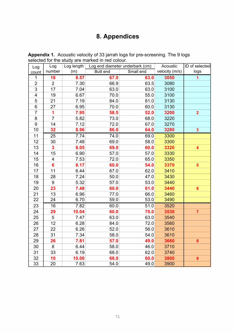
71
8. Appendices Appendix 1. Acoustic velocity of 33 jarrah logs for pre-screening. The 9 logs selected for the study are marked in red colour.
Butt end Small end
1 18 8.57 67.0 63.0 3050 12 2 7.30 66.9 63.5 30803 17 7.04 63.0 63.0 31004 19 6.67 70.0 55.0 31005 21 7.19 84.0 81.0 31306 27 6.95 70.0 60.0 31307 1 7.95 58.5 52.0 3200 28 7 5.82 73.0 68.0 32209 14 7.12 72.0 67.0 327010 32 8.96 86.0 64.0 3280 311 25 7.74 74.0 69.0 330012 30 7.48 69.0 58.0 330013 3 8.05 69.0 60.0 3320 414 15 6.90 57.0 57.0 333015 4 7.53 72.0 65.0 335016 6 8.17 60.0 54.0 3370 517 11 6.44 67.0 62.0 341018 28 7.24 50.0 47.0 343019 9 5.32 57.0 53.0 344020 23 7.48 60.0 61.0 3440 621 13 6.96 77.0 66.0 346022 24 6.70 59.0 53.0 349023 16 7.82 60.0 51.0 352024 29 10.04 60.0 70.0 3530 725 5 7.47 63.0 63.0 354026 12 6.28 84.0 72.0 356027 22 6.26 52.0 56.0 361028 31 7.34 58.0 54.0 361029 26 7.81 57.0 49.0 3660 830 8 6.44 58.0 46.0 371031 33 6.19 68.0 62.0 374032 10 10.00 68.0 60.0 3800 933 20 7.63 54.0 49.0 3900
ID of selected logs
Log end diameter underbark (cm) Acoustic velocity (m/s)
Log count
Log number
Log length (m)
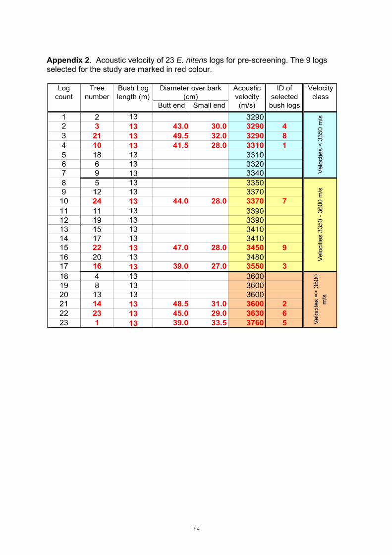
72
Appendix 2. Acoustic velocity of 23 E. nitens logs for pre-screening. The 9 logs selected for the study are marked in red colour.
Butt end Small end
1 2 13 32902 3 13 43.0 30.0 3290 43 21 13 49.5 32.0 3290 84 10 13 41.5 28.0 3310 15 18 13 33106 6 13 33207 9 13 33408 5 13 33509 12 13 337010 24 13 44.0 28.0 3370 711 11 13 339012 19 13 339013 15 13 341014 17 13 341015 22 13 47.0 28.0 3450 916 20 13 348017 16 13 39.0 27.0 3550 318 4 13 360019 8 13 360020 13 13 360021 14 13 48.5 31.0 3600 222 23 13 45.0 29.0 3630 623 1 13 39.0 33.5 3760 5
Log count
Vel
ocite
s =
> 3
500
m/s
Vel
ociti
es 3
350
- 36
00 m
/sV
eloc
ties
< 3
350
m/s
Acoustic velocity (m/s)
Velocity class
ID of selected
bush logs
Tree number
Bush Log length (m)
Diameter over bark (cm)

73
Appendix 3. The NIR spectra of one jarrah specimen.
Appendix 4. The NIR spectra of one E. nitens specimen.

74
Appendix 5. Ultrasonic velocities of 54 green block specimens of jarrah.
Shear Wave Velocities (m/s)
L R T
Mean VLL
Mean VXX
Mean VWW
Mean VLR
Mean VLT
Mean VXL
Mean VXW
Mean VWL
Mean VWX
1111 50.4 56.1 114.6 1196 10 3583 2104 1974 1001 809 938 646 869 6481112 50.7 56.9 114.1 1160 8 3746 2007 1505 1026 816 1020 663 828 6351113 49.8 54.9 114.1 1229 0 3380 2100 2041 995 779 903 632 719 5951131 50.0 56.7 114.4 1219 3 3713 2021 1853 993 821 948 702 849 5561132 48.9 55.8 114.7 1246 3 3578 2133 1951 1016 836 933 674 897 6681133 49.4 56.3 115.1 1254 5 3384 2164 2112 1054 832 1027 773 774 6821211 50.5 113.8 57.5 1070 60 3807 1646 1789 963 807 880 610 884 5271212 49.2 58.1 114.0 1073 22 3433 1770 1698 938 821 925 640 761 5941213 51.0 56.8 113.7 1077 5 3626 1846 1543 966 799 919 612 837 5131231 49.4 114.0 56.8 1078 60 3921 1695 1677 951 845 881 595 852 5491232 49.3 57.4 113.7 1050 35 3872 1700 1669 954 867 929 632 802 5931233 49.5 56.6 114.0 1064 5 3808 1817 1519 966 813 916 623 821 5651311 53.1 56.6 114.7 1058 5 3739 1820 1545 1033 797 931 530 826 4521312 54.6 56.7 114.5 1131 10 3809 1940 1771 1028 787 1054 546 764 4661313 53.2 57.2 114.6 1136 12 3782 1917 1717 1001 827 926 623 820 4881331 50.1 55.7 114.0 1095 5 3894 1849 1519 1011 802 931 526 756 4561332 48.9 57.5 114.7 1147 0 3762 1986 1736 1043 829 962 594 820 5521333 50.5 56.2 115.0 1120 10 4051 1875 1656 997 837 924 612 768 5481411 50.8 113.5 57.5 1110 50 3629 1801 1844 940 726 801 636 861 6081412 49.9 56.6 114.4 1161 0 3297 2065 1890 957 665 1052 623 764 6471413 50.2 55.7 113.8 1165 6 3407 2066 1782 902 784 873 612 797 6261431 48.8 113.1 57.4 1102 85 3957 1622 1956 1021 790 751 616 878 5961432 49.2 58.0 113.6 1115 15 4193 1904 1544 1029 792 970 639 739 5861433 49.4 57.9 113.7 1117 30 3941 1931 1761 1041 770 968 659 712 5931511 49.0 113.6 56.4 1174 60 3848 1834 1902 984 866 823 677 862 6461512 49.0 57.4 113.4 1190 0 3568 1896 1864 987 803 1051 677 714 5851513 49.7 53.9 114.0 1179 5 3637 1915 1895 975 853 1041 643 839 6271531 50.0 114.2 58.1 1185 65 3695 1837 1937 960 885 879 719 915 6321532 49.9 115.0 57.4 1214 60 3433 1931 2011 970 873 929 690 829 6471533 50.2 54.7 114.3 1209 15 3535 1974 1701 972 885 900 694 867 6151611 49.5 58.2 111.7 1039 5 3604 1807 1603 1075 898 1141 620 932 5821612 49.6 113.0 57.2 1100 45 3815 1777 1770 1105 902 1090 758 959 6901613 49.8 57.2 111.0 1113 5 3644 1909 1633 1107 878 1149 683 889 6621631 49.9 111.6 56.0 1112 45 3960 1834 1745 1032 890 926 663 916 6211632 49.0 56.7 111.7 1156 20 3848 1956 1916 1061 882 1078 690 874 6741633 49.3 58.0 111.4 1168 0 3915 2033 1759 1077 874 990 723 845 6641711 50.8 57.8 112.3 1148 20 3328 1977 1700 1000 780 1055 585 703 5981712 50.2 55.4 113.3 1161 0 3746 2075 1813 1039 799 1037 617 772 6071713 51.3 57.1 113.1 1159 25 3828 1978 1726 1030 818 924 672 865 6511731 52.1 56.7 113.0 1111 0 3850 1940 1583 964 828 948 536 877 4961732 50.8 58.1 113.5 1122 5 4032 1998 1780 1026 835 1080 669 795 5261733 50.4 56.9 112.7 1116 20 4177 1979 1635 1029 852 984 696 733 5421811 49.6 113.1 56.8 1169 60 4066 1873 1426 975 868 919 6891812 49.2 56.6 112.8 1202 40 3947 1981 1925 985 882 887 657 862 6271813 50.4 55.6 113.3 1208 20 4000 1999 1957 1001 875 911 633 915 6371831 49.3 113.3 57.1 1154 45 4178 1812 1855 916 834 890 648 793 5851832 50.0 57.3 113.2 1169 35 3807 1928 1852 991 847 958 692 8651833 49.8 54.7 113.5 1221 5 3773 2166 1745 961 892 1056 831 972 6421911 48.9 113.5 58.1 1178 55 3922 1916 1970 1062 838 940 693 917 6611912 48.8 57.2 114.4 1169 5 4044 2006 1731 1069 842 990 644 754 5561913 49.9 56.3 113.9 1176 10 3838 1993 1857 1062 838 991 664 8841931 48.8 57.8 113.1 1141 25 4231 1868 1784 1001 826 967 616 776 5721932 50.1 56.3 114.6 1151 5 4246 1952 1733 1060 853 974 620 755 5361933 49.6 58.6 113.8 1140 15 4066 1939 1886 1089 878 1014 708 838 619
Specimen ID
Longitudinal Wave Velocity (m/s)
Green Dimensions (mm)Green density (kg/m3)
Ring angle
(degree)
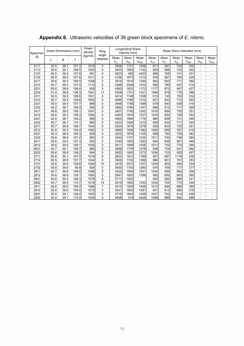
75
Appendix 6. Ultrasonic velocities of 36 green block specimens of E. nitens.
Shear Wave Velocities (m/s)
L R TMean VLL
Mean VXX
Mean VWW
Mean VLR
Mean VLT
Mean VXL
Mean VXW
Mean VWL
Mean VWX
2111 50.5 38.7 107.3 1018 5 3508 1727 1248 871 587 703 355 - -2112 50.6 39.1 108.5 1003 0 3833 1683 1142 920 666 723 340 - -2131 50.5 39.3 107.8 991 0 3823 465 4453 885 765 741 401 - -2132 50.9 39.5 107.6 1011 0 4106 1673 1312 878 661 790 425 - -2211 50.6 39.3 109.0 1058 3 3515 1819 1346 992 693 771 385 - -2212 50.7 39.4 107.5 1110 0 4368 2008 1433 994 780 937 419 - -2231 50.6 38.8 106.6 928 5 4363 1832 1172 1177 973 947 427 - -2232 51.0 38.8 106.3 1001 11 5308 1701 1251 1084 879 776 396 - -2311 50.5 39.2 108.6 1031 5 3414 1748 1309 815 743 783 332 - -2312 50.7 39.2 108.6 1053 0 4086 1780 1410 921 633 712 363 - -2331 50.5 39.4 107.7 869 0 3948 1758 1398 919 640 938 419 - -2332 50.2 38.7 108.0 995 0 3582 1760 1161 896 612 717 395 - -2411 49.8 39.0 108.1 1041 0 3457 1740 1242 1016 664 735 351 - -2412 50.6 39.3 108.3 1082 0 4363 1819 1337 1033 830 728 342 - -2431 50.5 38.7 108.2 989 0 3605 1669 1176 885 608 731 380 - -2432 50.7 39.1 110.1 990 0 4223 1656 1210 859 634 711 340 - -2511 50.7 38.9 108.7 1044 0 3424 1678 1278 938 603 735 351 - -2512 50.8 39.3 109.2 1082 0 3965 1928 1382 1080 695 787 419 - -2531 50.3 38.9 108.3 929 5 3222 1678 1105 898 750 735 382 - -2532 50.6 38.9 107.4 983 0 3242 1707 1235 1011 755 748 385 - -2611 50.6 39.4 107.3 953 0 3160 1825 1263 954 648 961 448 - -2612 50.6 39.5 109.1 1055 0 3511 1898 1436 1011 702 774 395 - -2631 50.7 39.1 108.7 960 0 3958 1778 1278 938 724 931 460 - -2632 50.6 38.9 108.2 994 0 3832 1800 1273 1054 723 925 457 - -2711 50.8 39.1 107.0 1019 6 2823 1812 1189 907 687 1118 435 - -2712 50.5 38.8 107.7 1044 5 3506 1732 1298 886 801 761 353 - -2731 50.6 39.0 108.6 1009 10 3416 2072 1357 1204 803 950 534 - -2732 50.8 38.8 95.8 928 0 3630 1703 1260 876 706 777 377 - -2811 50.7 38.8 108.6 1086 5 3422 1900 1551 1034 694 862 356 - -2812 50.6 38.8 109.1 1060 0 2941 1903 1398 992 693 863 360 - -2831 50.6 39.2 106.3 1078 8 3717 1920 954 692 890 421 - -2832 50.7 39.4 110.7 1018 14 3519 1825 1333 1034 704 773 346 - -2911 50.6 39.0 108.3 1066 7 3515 1839 1406 1012 684 886 390 - -2912 50.8 39.0 109.0 1070 5 3341 1803 1397 941 612 885 378 - -2931 50.5 39.1 108.4 1000 0 3716 1844 1408 1031 702 814 439 - -2932 50.5 39.1 110.0 1039 0 4508 579 5448 1098 886 952 488 - -
Specimen ID
Longitudinal Wave Velocity (m/s)
Green Dimensions (mm)Green density (kg/m3)
Ring angle
(degree)

76
Appendix 7. Acoustic tomograph (map of radial velocities) of jarrah.
(to continue)
Bush log 1 Bush log 2
Bush log 3 Bush log 4
Bush log 5 Bush log 6
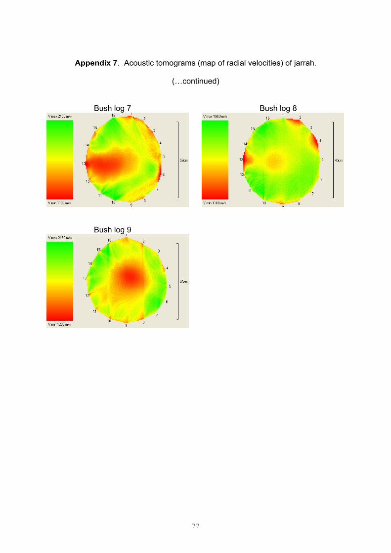
77
Appendix 7. Acoustic tomograms (map of radial velocities) of jarrah.
(…continued)
Bush log 7 Bush log 8
Bush log 9

78
Appendix 8. Acoustic tomograms (map of radial velocities) of E. nitens.
(to continue)
Bush log 1A Bush log 2A
Bush log 1B Bush log 2B
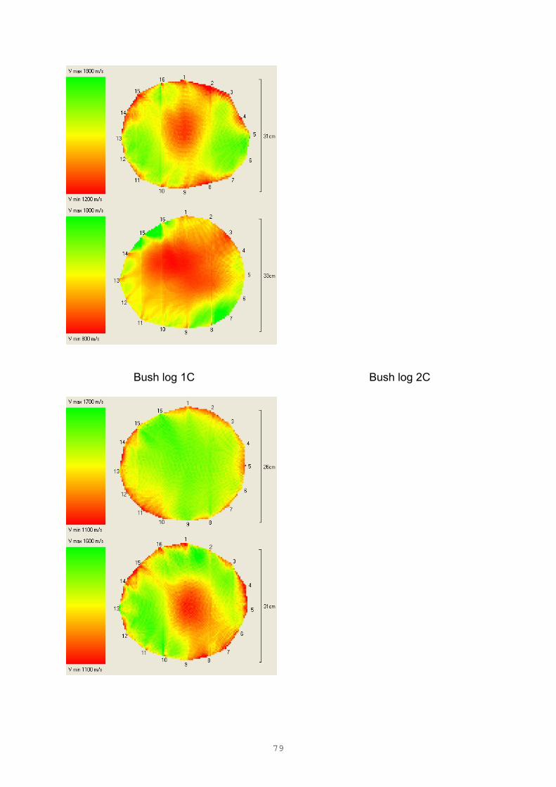
79
Bush log 1C Bush log 2C

80
Appendix 8. Acoustic tomograms (map of radial velocities) of E. nitens.
(…continued) Bush log 3A Bush log 4A
Bush log 3B Bush log 4B
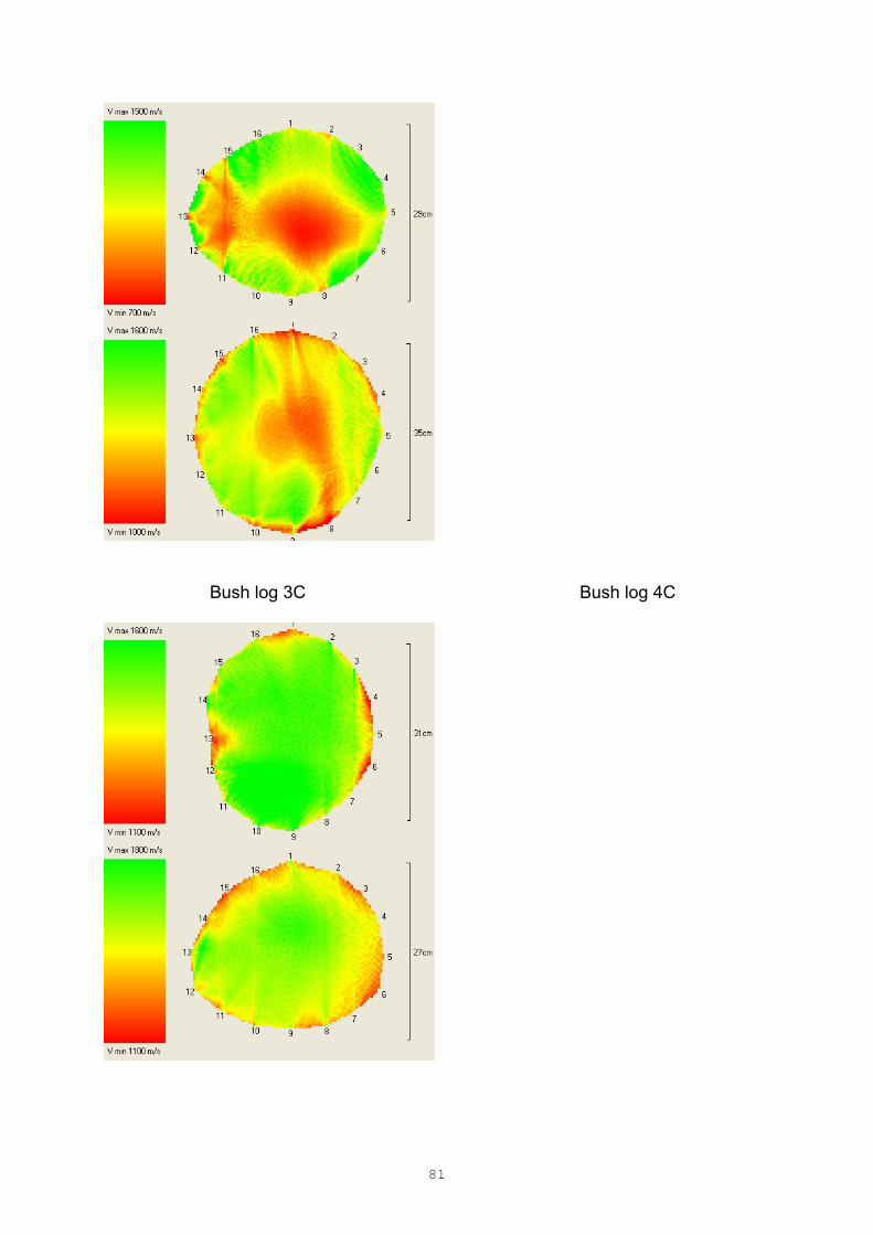
81
Bush log 3C Bush log 4C

82
Appendix 8. Acoustic tomograms (map of radial velocities) of E. nitens.
(…continued)
Bush log 5A Bush log 6A
Bush log 5B Bush log 6B
Bush log 5C Bush log 6C
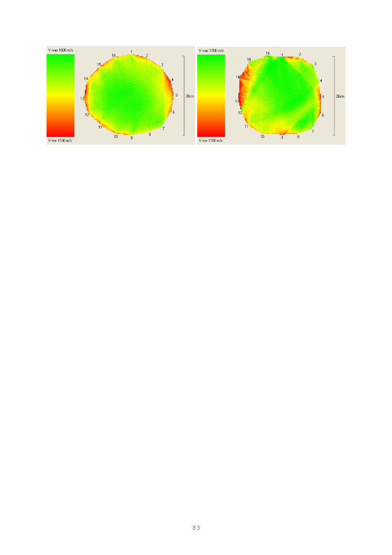
83

84
Appendix 8. Acoustic tomograms (map of radial velocities) of E. nitens.
(…continued)
Bush log 7A Bush log 8A
Bush log 7B Bush log 8B
Bush log 7C Bush log 8C

85
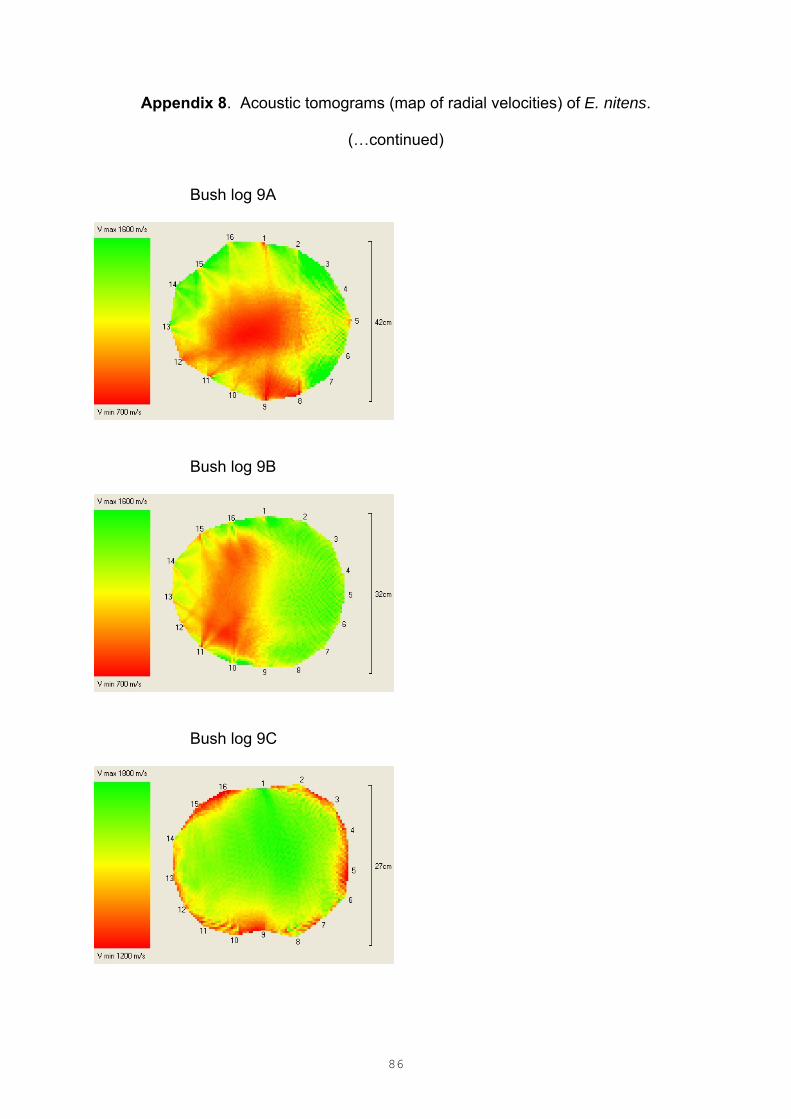
86
Appendix 8. Acoustic tomograms (map of radial velocities) of E. nitens.
(…continued)
Bush log 9A
Bush log 9B
Bush log 9C

87
Appendix 9. Initial moisture content, basic density, and extractive contents of jarrah. (to continue)

88
Appendix 9. Initial moisture content, basic density, and extractive contents of jarrah. (…continued)

89
Appendix 10. Moisture content, basic density, and extractive contents of E. nitens
(to continue…)
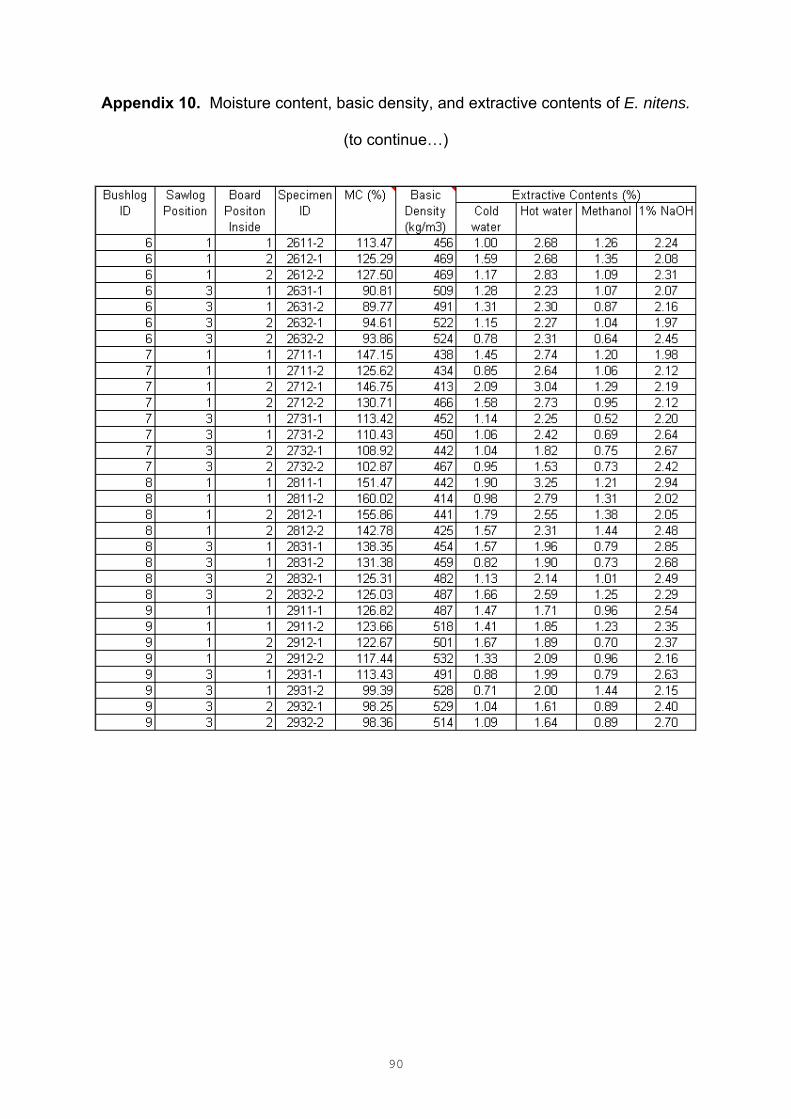
90
Appendix 10. Moisture content, basic density, and extractive contents of E. nitens.
(to continue…)
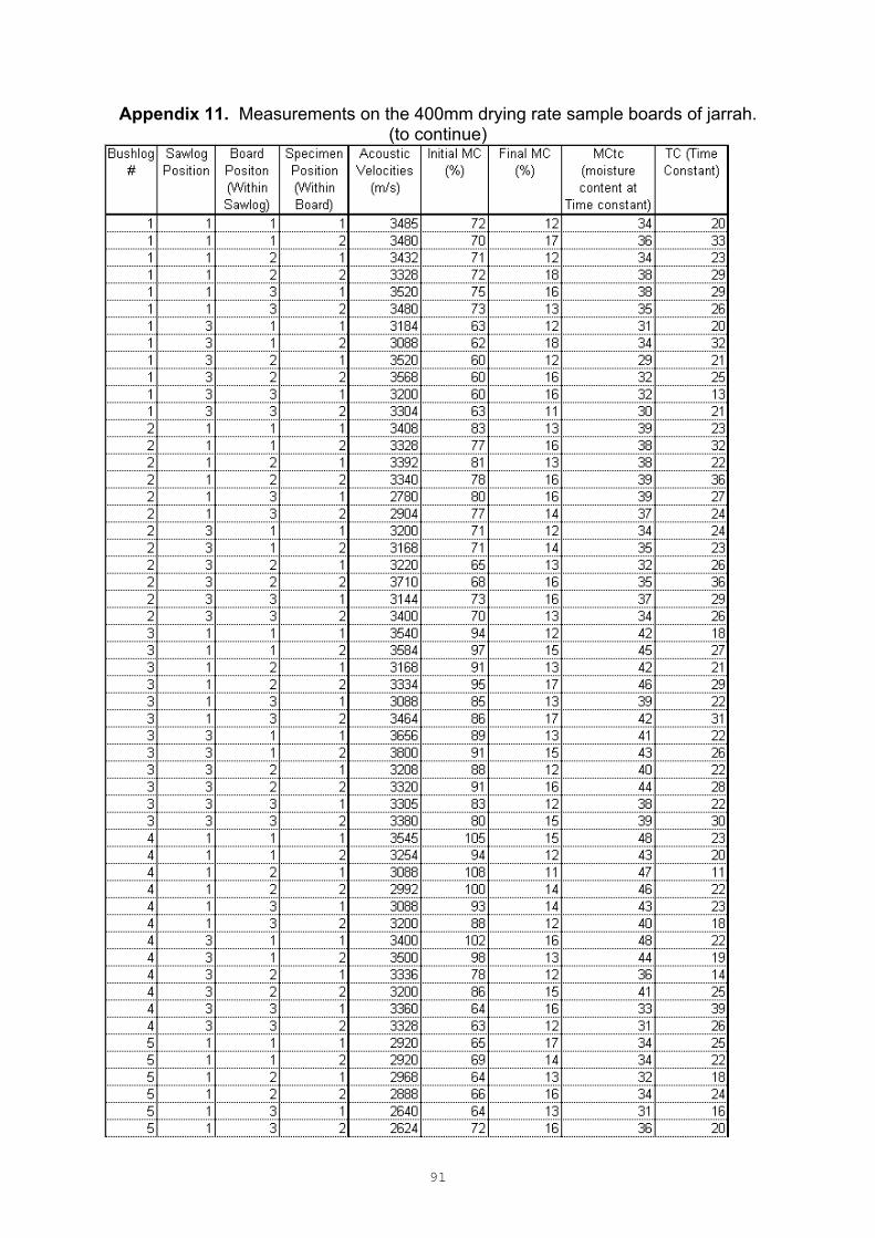
91
Appendix 11. Measurements on the 400mm drying rate sample boards of jarrah. (to continue)

92
Appendix 11. Measurements on the 400mm drying rate sample boards of jarrah. (… continued)
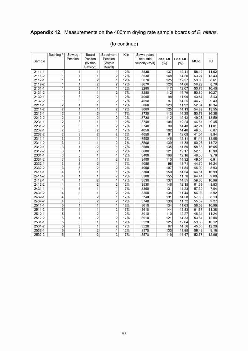
93
Appendix 12. Measurements on the 400mm drying rate sample boards of E. nitens.
(to continue)
Sample
Bushlog # Sawlog Position
Board Positon (Within Sawlog)
Specimen Position (Within Board)
Kiln Sawn board acoustic
velocity (m/s)Initial MC
(%)Final MC
(%)MCtc TC
2111-1 1 1 1 1 12% 3530 137 12.11 58.12 11.622111-2 1 1 1 2 17% 3530 148 14.20 63.27 13.432112-1 1 1 2 1 12% 3670 125 12.27 53.86 8.612112-2 1 1 2 2 17% 3670 128 14.66 56.29 8.792131-1 1 3 1 1 12% 3280 117 12.07 50.76 10.402131-2 1 3 1 2 17% 3280 112 14.79 50.60 10.272132-1 1 3 2 1 12% 4090 98 11.99 43.57 8.432132-2 1 3 2 2 17% 4090 97 14.25 44.70 9.432211-1 2 1 1 1 12% 3060 123 11.92 52.64 10.342211-2 2 1 1 2 17% 3060 125 14.13 54.89 13.552212-1 2 1 2 1 17% 3730 113 14.28 50.73 16.362212-2 2 1 2 2 12% 3730 112 12.43 49.25 13.592231-1 2 3 1 1 12% 3740 106 12.24 46.81 9.452231-2 2 3 1 2 17% 3740 90 14.48 42.24 11.012232-1 2 3 2 1 17% 4050 102 14.40 46.58 6.872232-2 2 3 2 2 12% 4050 91 12.08 41.01 8.942311-1 3 1 1 1 12% 3500 146 12.11 61.41 13.062311-2 3 1 1 2 17% 3500 139 14.38 60.25 14.722312-1 3 1 2 1 17% 3680 135 14.50 58.85 16.652312-2 3 1 2 2 12% 3680 121 12.17 52.16 15.992331-1 3 3 1 1 12% 3400 106 12.16 46.56 9.792331-2 3 3 1 2 17% 3400 110 14.32 49.51 6.912332-1 3 3 2 1 17% 4050 98 13.71 44.70 16.242332-2 3 3 2 2 12% 4050 107 11.84 46.90 8.932411-1 4 1 1 1 17% 3300 150 14.54 64.54 10.992411-2 4 1 1 2 12% 3300 155 11.78 64.44 9.092412-1 4 1 2 1 17% 3530 137 14.55 59.65 10.992412-2 4 1 2 2 12% 3530 146 12.15 61.39 8.832431-1 4 3 1 1 17% 3360 131 14.23 57.30 7.042431-2 4 3 1 2 12% 3360 135 11.44 56.98 5.922432-1 4 3 2 1 17% 3740 131 14.58 57.55 8.132432-2 4 3 2 2 12% 3740 130 11.72 55.32 9.272511-1 5 1 1 1 12% 3610 134 11.63 56.53 10.992511-2 5 1 1 2 17% 3610 144 13.83 61.67 11.382512-1 5 1 2 1 12% 3910 110 12.27 48.34 11.242512-2 5 1 2 2 17% 3910 121 14.33 53.67 12.062531-1 5 3 1 1 12% 3520 125 12.04 53.63 10.122531-2 5 3 1 2 17% 3520 97 14.56 45.06 12.292532-1 5 3 2 1 12% 3570 133 11.85 56.42 9.162532-2 5 3 2 2 17% 3570 119 14.47 52.78 12.06
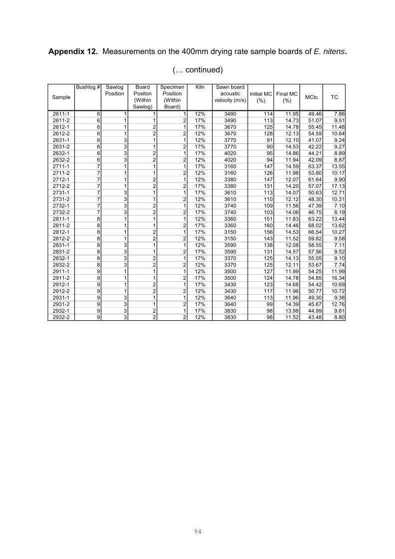
94
Appendix 12. Measurements on the 400mm drying rate sample boards of E. nitens.
(… continued)
Sample
Bushlog # Sawlog Position
Board Positon (Within Sawlog)
Specimen Position (Within Board)
Kiln Sawn board acoustic
velocity (m/s)Initial MC
(%)Final MC
(%)MCtc TC
2611-1 6 1 1 1 12% 3490 114 11.95 49.46 7.862611-2 6 1 1 2 17% 3490 113 14.73 51.07 9.512612-1 6 1 2 1 17% 3670 125 14.78 55.45 11.482612-2 6 1 2 2 12% 3670 128 12.13 54.59 10.642631-1 6 3 1 1 12% 3770 91 12.10 41.07 9.242631-2 6 3 1 2 17% 3770 90 14.53 42.22 9.272632-1 6 3 2 1 17% 4020 95 14.86 44.21 8.892632-2 6 3 2 2 12% 4020 94 11.94 42.09 8.872711-1 7 1 1 1 17% 3160 147 14.59 63.37 13.552711-2 7 1 1 2 12% 3160 126 11.98 53.80 10.172712-1 7 1 2 1 12% 3380 147 12.07 61.64 9.902712-2 7 1 2 2 17% 3380 131 14.20 57.07 17.132731-1 7 3 1 1 17% 3610 113 14.07 50.63 12.712731-2 7 3 1 2 12% 3610 110 12.12 48.30 10.312732-1 7 3 2 1 12% 3740 109 11.56 47.39 7.102732-2 7 3 2 2 17% 3740 103 14.06 46.75 8.192811-1 8 1 1 1 12% 3360 151 11.83 63.22 13.442811-2 8 1 1 2 17% 3360 160 14.46 68.02 13.622812-1 8 1 2 1 17% 3150 156 14.53 66.54 10.272812-2 8 1 2 2 12% 3150 143 11.52 59.82 9.582831-1 8 3 1 1 12% 3590 138 12.08 58.55 7.112831-2 8 3 1 2 17% 3590 131 14.57 57.56 9.522832-1 8 3 2 1 17% 3370 125 14.13 55.05 9.102832-2 8 3 2 2 12% 3370 125 12.11 53.67 7.742911-1 9 1 1 1 12% 3500 127 11.99 54.25 11.992911-2 9 1 1 2 17% 3500 124 14.78 54.85 16.342912-1 9 1 2 1 17% 3430 123 14.68 54.42 10.692912-2 9 1 2 2 12% 3430 117 11.96 50.77 10.722931-1 9 3 1 1 12% 3640 113 11.96 49.30 9.382931-2 9 3 1 2 17% 3640 99 14.39 45.67 12.762932-1 9 3 2 1 17% 3830 98 13.98 44.99 9.812932-2 9 3 2 2 12% 3830 98 11.52 43.48 8.80

95
Appendix 13. Shrinkage, collapse and internal checks of jarrah. (to continue)
Bushlog #
Sawlog Position
Board Positon (Within Sawlog)
Specimen Position (Within Board)
Total area shrinkage
(less area of internal
checks), %
Total area shrinkage (%) (Image analysis)
Collapse (%)
Number of checks in range
Total area of checks (mm2)
1 1 1 1 19.3 9.0 10.3 6 45.571 1 1 2 22.0 8.9 13.1 7 17.171 1 2 1 17.1 9.2 7.9 4 12.271 1 2 2 21.1 8.8 12.3 9 5.791 1 3 1 17.4 8.5 8.9 3 24.361 1 3 2 16.0 8.0 8.0 5 15.111 3 1 1 21.9 11.3 10.6 11 19.581 3 1 2 30.9 15.1 15.8 2 0.491 3 2 1 25.6 10.7 14.9 16 84.671 3 2 2 27.9 14.7 13.2 0 0.001 3 3 1 15.0 9.1 5.9 2 6.331 3 3 2 20.1 8.4 11.7 8 25.112 1 1 1 32.0 10.4 21.6 1 0.132 1 1 2 33.6 11.2 22.4 0 0.002 1 2 1 25.1 10.5 14.6 4 8.212 1 2 2 29.9 9.7 20.2 1 0.252 1 3 1 19.6 11.9 7.7 0 0.002 1 3 2 24.9 13.1 11.8 1 1.182 3 1 1 33.1 14.6 18.5 2 15.222 3 1 2 32.3 12.4 19.9 1 0.052 3 2 1 26.3 11.5 14.8 1 5.502 3 2 2 27.1 11.5 15.6 0 0.002 3 3 1 25.8 11.5 14.3 0 0.002 3 3 2 23.2 9.7 13.5 2 20.733 1 1 1 19.2 9.7 9.5 7 25.683 1 1 2 22.9 11.2 11.7 3 22.643 1 2 1 19.5 9.2 10.3 10 19.983 1 2 2 28.1 11.0 17.1 10 2.103 1 3 1 18.6 9.1 9.5 7 27.563 1 3 2 22.9 10.0 12.9 8 27.293 3 1 1 26.3 12.5 13.8 14 36.593 3 1 2 31.1 14.7 16.4 7 15.773 3 2 1 29.6 12.0 17.6 9 9.113 3 2 2 32.9 10.9 22.0 12 11.723 3 3 1 28.8 9.6 19.2 13 59.893 3 3 2 25.2 9.5 15.7 8 55.624 1 1 1 14.1 8.0 6.1 0 0.004 1 1 2 13.5 7.4 6.1 1 0.314 1 2 1 12.8 7.2 5.6 10 14.934 1 2 2 12.2 8.6 3.6 4 3.514 1 3 1 11.4 7.9 3.5 0 0.004 1 3 2 11.4 7.6 3.8 0 0.004 3 1 1 13.0 7.9 5.1 0 0.004 3 1 2 13.3 8.2 5.1 0 0.004 3 2 1 17.3 10.0 7.3 1 5.424 3 2 2 12.9 8.6 4.3 0 0.004 3 3 1 12.2 7.7 4.5 0 0.004 3 3 2 10.6 8.1 2.5 0 0.005 1 1 1 25.4 13.1 12.3 1 0.215 1 1 2 31.3 13.4 17.9 4 3.245 1 2 1 24.1 12.9 11.2 6 22.965 1 2 2 29.1 13.8 15.3 6 4.305 1 3 1 18.4 12.2 6.2 12 43.135 1 3 2 28.3 12.4 15.9 3 0.24
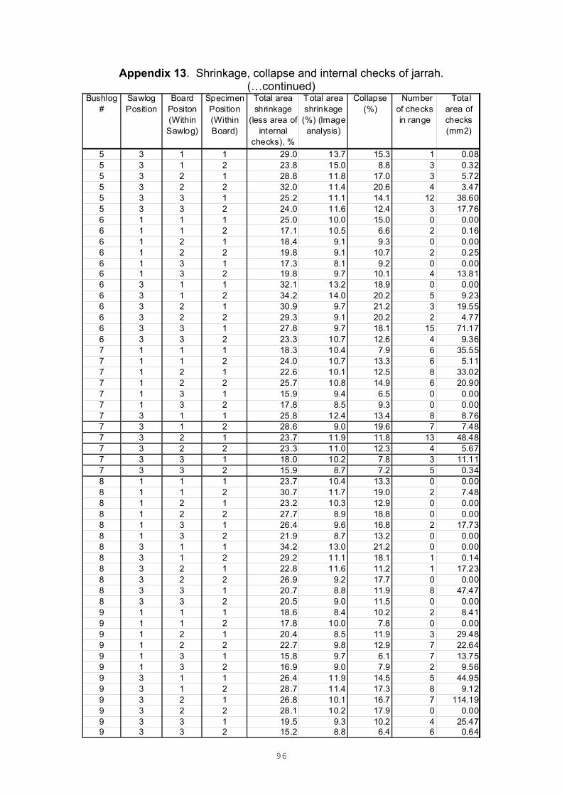
96
Appendix 13. Shrinkage, collapse and internal checks of jarrah. (…continued)
Bushlog #
Sawlog Position
Board Positon (Within Sawlog)
Specimen Position (Within Board)
Total area shrinkage
(less area of internal
checks), %
Total area shrinkage (%) (Image analysis)
Collapse (%)
Number of checks in range
Total area of checks (mm2)
5 3 1 1 29.0 13.7 15.3 1 0.085 3 1 2 23.8 15.0 8.8 3 0.325 3 2 1 28.8 11.8 17.0 3 5.725 3 2 2 32.0 11.4 20.6 4 3.475 3 3 1 25.2 11.1 14.1 12 38.605 3 3 2 24.0 11.6 12.4 3 17.766 1 1 1 25.0 10.0 15.0 0 0.006 1 1 2 17.1 10.5 6.6 2 0.166 1 2 1 18.4 9.1 9.3 0 0.006 1 2 2 19.8 9.1 10.7 2 0.256 1 3 1 17.3 8.1 9.2 0 0.006 1 3 2 19.8 9.7 10.1 4 13.816 3 1 1 32.1 13.2 18.9 0 0.006 3 1 2 34.2 14.0 20.2 5 9.236 3 2 1 30.9 9.7 21.2 3 19.556 3 2 2 29.3 9.1 20.2 2 4.776 3 3 1 27.8 9.7 18.1 15 71.176 3 3 2 23.3 10.7 12.6 4 9.367 1 1 1 18.3 10.4 7.9 6 35.557 1 1 2 24.0 10.7 13.3 6 5.117 1 2 1 22.6 10.1 12.5 8 33.027 1 2 2 25.7 10.8 14.9 6 20.907 1 3 1 15.9 9.4 6.5 0 0.007 1 3 2 17.8 8.5 9.3 0 0.007 3 1 1 25.8 12.4 13.4 8 8.767 3 1 2 28.6 9.0 19.6 7 7.487 3 2 1 23.7 11.9 11.8 13 48.487 3 2 2 23.3 11.0 12.3 4 5.677 3 3 1 18.0 10.2 7.8 3 11.117 3 3 2 15.9 8.7 7.2 5 0.348 1 1 1 23.7 10.4 13.3 0 0.008 1 1 2 30.7 11.7 19.0 2 7.488 1 2 1 23.2 10.3 12.9 0 0.008 1 2 2 27.7 8.9 18.8 0 0.008 1 3 1 26.4 9.6 16.8 2 17.738 1 3 2 21.9 8.7 13.2 0 0.008 3 1 1 34.2 13.0 21.2 0 0.008 3 1 2 29.2 11.1 18.1 1 0.148 3 2 1 22.8 11.6 11.2 1 17.238 3 2 2 26.9 9.2 17.7 0 0.008 3 3 1 20.7 8.8 11.9 8 47.478 3 3 2 20.5 9.0 11.5 0 0.009 1 1 1 18.6 8.4 10.2 2 8.419 1 1 2 17.8 10.0 7.8 0 0.009 1 2 1 20.4 8.5 11.9 3 29.489 1 2 2 22.7 9.8 12.9 7 22.649 1 3 1 15.8 9.7 6.1 7 13.759 1 3 2 16.9 9.0 7.9 2 9.569 3 1 1 26.4 11.9 14.5 5 44.959 3 1 2 28.7 11.4 17.3 8 9.129 3 2 1 26.8 10.1 16.7 7 114.199 3 2 2 28.1 10.2 17.9 0 0.009 3 3 1 19.5 9.3 10.2 4 25.479 3 3 2 15.2 8.8 6.4 6 0.64

97
Appendix 14. Shrinkage, collapse and internal checks of E. nitens.
(to continue)
Bushlog #
Sawlog Position
Board Positon (Within Sawlog)
Specimen Position (Within Board)
Total area shrinkage
(less area of internal
checks), %
Total area shrinkage (%) (Image analysis)
Collapse (%)
Number of checks in range
Total area of checks (mm2)
1 1 1 1 21.99 7.12 14.87 47 128.231 1 1 2 19.82 7.35 12.47 65 122.221 1 2 1 25.62 7.89 17.73 21 95.271 1 2 2 23.42 8.20 15.22 30 85.571 3 1 1 12.09 7.95 4.14 23 24.551 3 1 2 12.30 8.40 3.91 11 6.671 3 2 1 15.23 10.24 4.99 8 22.101 3 2 2 15.14 10.63 4.51 0 02 1 1 1 7.482 1 1 2 14.94 7.76 7.18 59 97.222 1 2 1 29.82 8.99 20.83 42 213.642 1 2 2 20.38 9.02 11.36 24 118.392 3 1 1 13.29 6.97 6.32 5 11.212 3 1 2 7.38 7.86 -0.48 3 2.002 3 2 1 15.28 9.77 5.51 15 15.692 3 2 2 13.20 10.40 2.80 1 0.153 1 1 1 11.70 6.11 5.59 16 41.293 1 1 2 12.30 6.61 5.69 13 17.453 1 2 1 21.67 7.68 13.98 21 132.473 1 2 2 19.59 8.30 11.29 17 60.263 3 1 1 9 03 3 1 2 -0.99 6.26 -7.26 0 03 3 2 1 9.10 8.50 0.59 2 03 3 2 2 8.24 9.28 -1.04 3 17.734 1 1 1 15.97 5.88 10.09 9 14.134 1 1 2 12.89 6.11 6.78 2 20.274 1 2 1 21.22 7.37 13.85 3 2.964 1 2 2 18.87 7.57 11.30 4 0.724 3 1 1 7.46 5.42 2.05 0 04 3 1 2 8.41 5.25 3.16 1 2.734 3 2 1 13.10 6.48 6.62 0 04 3 2 2 10.19 5.81 4.37 0 05 1 1 1 13.68 7.49 6.19 59 81.485 1 1 2 16.05 6.60 9.45 50 106.805 1 2 1 20.30 9.58 10.72 51 160.235 1 2 2 20.60 7.88 12.72 46 191.915 3 1 1 8.51 5.27 3.24 10 7.685 3 1 2 8.82 4.83 3.99 7 11.385 3 2 1 16.98 5.95 11.03 16 26.515 3 2 2 15.20 5.79 9.42 8 8.75
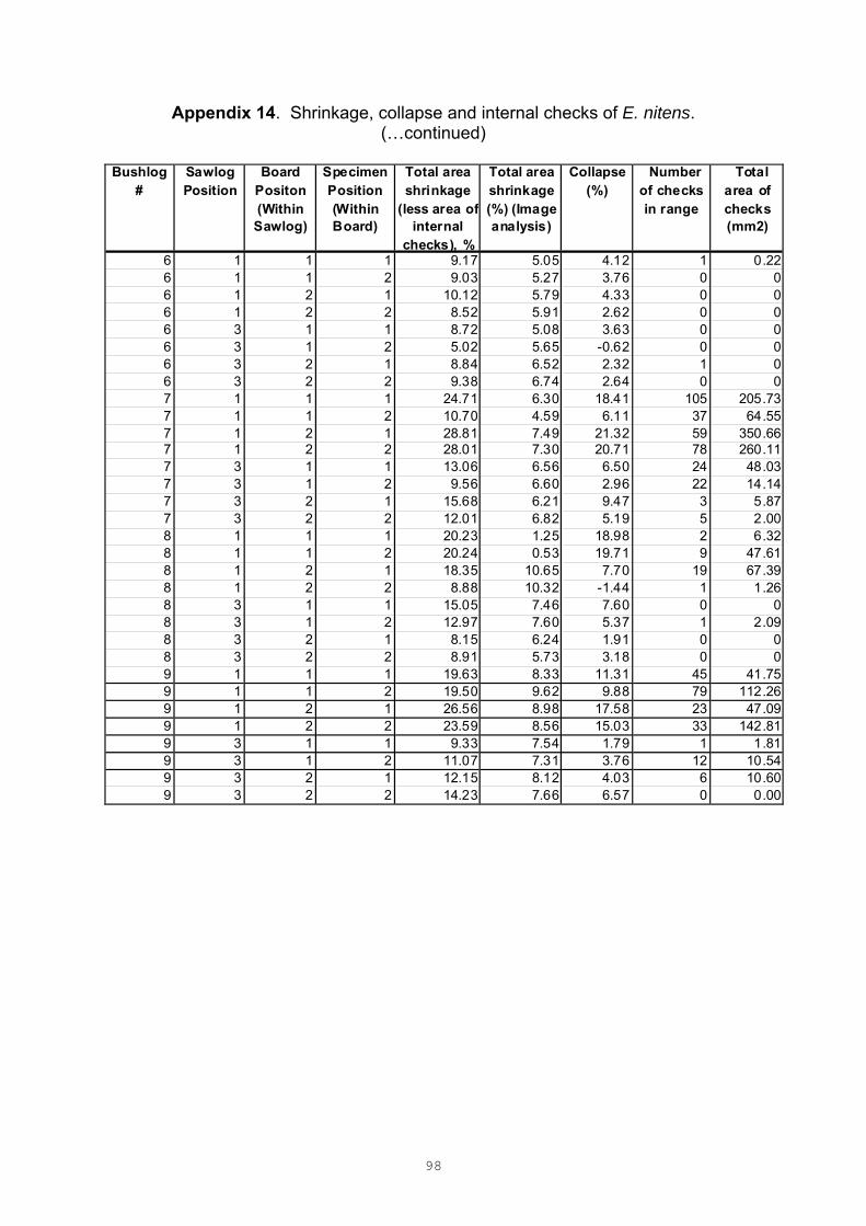
98
Appendix 14. Shrinkage, collapse and internal checks of E. nitens. (…continued)
Bushlog
#Sawlog Position
Board Positon (Within Sawlog)
Specimen Position (Within Board)
Total area shrinkage
(less area of internal
checks), %
Total area shrinkage (%) (Image analysis)
Collapse (%)
Number of checks in range
Total area of checks (mm2)
6 1 1 1 9.17 5.05 4.12 1 0.226 1 1 2 9.03 5.27 3.76 0 06 1 2 1 10.12 5.79 4.33 0 06 1 2 2 8.52 5.91 2.62 0 06 3 1 1 8.72 5.08 3.63 0 06 3 1 2 5.02 5.65 -0.62 0 06 3 2 1 8.84 6.52 2.32 1 06 3 2 2 9.38 6.74 2.64 0 07 1 1 1 24.71 6.30 18.41 105 205.737 1 1 2 10.70 4.59 6.11 37 64.557 1 2 1 28.81 7.49 21.32 59 350.667 1 2 2 28.01 7.30 20.71 78 260.117 3 1 1 13.06 6.56 6.50 24 48.037 3 1 2 9.56 6.60 2.96 22 14.147 3 2 1 15.68 6.21 9.47 3 5.877 3 2 2 12.01 6.82 5.19 5 2.008 1 1 1 20.23 1.25 18.98 2 6.328 1 1 2 20.24 0.53 19.71 9 47.618 1 2 1 18.35 10.65 7.70 19 67.398 1 2 2 8.88 10.32 -1.44 1 1.268 3 1 1 15.05 7.46 7.60 0 08 3 1 2 12.97 7.60 5.37 1 2.098 3 2 1 8.15 6.24 1.91 0 08 3 2 2 8.91 5.73 3.18 0 09 1 1 1 19.63 8.33 11.31 45 41.759 1 1 2 19.50 9.62 9.88 79 112.269 1 2 1 26.56 8.98 17.58 23 47.099 1 2 2 23.59 8.56 15.03 33 142.819 3 1 1 9.33 7.54 1.79 1 1.819 3 1 2 11.07 7.31 3.76 12 10.549 3 2 1 12.15 8.12 4.03 6 10.609 3 2 2 14.23 7.66 6.57 0 0.00

99
Appendix 15. Shrinkage potential and shrinkages in oven-dry sections of jarrah. (to continue)
Shrinkage Width (%) 12%MC
Shrinkage Thick (%) 12%MC
MC % Width shrinkage
(%)
Thickness shrinkae
(%)
Area shrinkage
(%)
1 1 1 1 68.40 10.52 11.69 20.981 1 1 2 64.22 12.07 10.63 21.411 1 2 1 68.30 10.89 11.63 21.251 1 2 2 69.96 8.90 7.95 16.141 1 3 1 70.64 10.06 7.98 17.231 1 3 2 67.96 9.66 6.31 15.361 3 1 1 61.12 7.52 9.80 16.591 3 1 2 58.37 8.87 9.49 17.521 3 2 1 59.18 6.06 8.21 13.781 3 2 2 57.48 8.91 9.50 17.571 3 3 1 58.45 7.71 6.43 13.641 3 3 2 62.71 7.75 7.05 14.252 1 1 1 78.05 8.62 10.19 17.942 1 1 2 76.86 7.98 11.97 18.992 1 2 1 77.65 10.96 8.88 18.862 1 2 2 75.77 11.02 9.27 19.262 1 3 1 76.61 10.73 9.09 18.852 1 3 2 77.74 10.01 10.79 19.722 3 1 1 67.04 10.65 14.04 23.192 3 1 2 64.34 13.24 11.35 23.092 3 2 1 62.12 10.20 10.08 19.252 3 2 2 65.00 11.13 10.23 20.222 3 3 1 70.91 10.82 9.39 19.202 3 3 2 67.67 9.21 9.42 17.763 1 1 1 92.10 12.97 8.40 20.283 1 1 2 91.98 13.18 8.56 20.613 1 2 1 90.70 10.19 7.88 17.273 1 2 2 90.98 15.05 9.27 22.923 1 3 1 84.16 11.22 9.10 19.303 1 3 2 83.46 6.40 9.55 15.343 3 1 1 86.54 15.12 10.47 24.013 3 1 2 86.93 11.30 8.44 18.783 3 2 1 85.42 14.57 9.94 23.073 3 2 2 88.32 14.68 11.01 24.073 3 3 1 76.70 12.44 9.31 20.603 3 3 2 76.05 12.05 9.63 20.524 1 1 1 92.49 7.55 10.65 17.394 1 1 2 80.86 6.11 7.11 12.784 1 2 1 5.31 0.05 89.08 7.53 4.94 12.104 1 2 2 84.40 7.62 4.94 12.194 1 3 1 79.58 8.20 5.47 13.234 1 3 2 81.86 8.36 5.57 13.474 3 1 1 76.10 6.09 10.28 15.744 3 1 2 77.04 7.73 10.07 17.034 3 2 1 70.05 9.18 8.13 16.574 3 2 2 77.44 7.75 9.04 16.094 3 3 1 66.95 7.06 5.04 11.744 3 3 2 71.40 5.74 7.85 13.135 1 1 1 60.72 10.90 17.68 26.665 1 1 2 62.40 11.59 17.94 27.455 1 2 1 60.26 16.58 10.59 25.425 1 2 2 62.46 19.25 11.72 28.715 1 3 1 64.39 16.26 9.86 24.525 1 3 2 66.82 10.14 10.03 19.15
Shrinkage Potential Oven-dry 2mm sectionsBushlog # Sawlog Position
Board Positon (Within Sawlog)
Specimen Position (Within Board)
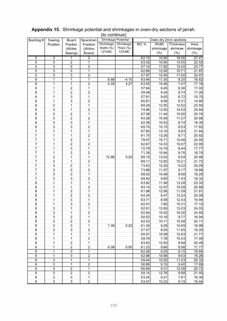
100
Appendix 15. Shrinkage potential and shrinkages in oven-dry sections of jarrah. (to continue)
Shrinkage Width (%) 12%MC
Shrinkage Thick (%) 12%MC
MC % Width shrinkage
(%)
Thickness shrinkae
(%)
Area shrinkage
(%)
5 3 1 2 62.15 10.95 18.56 27.475 3 2 1 63.32 10.90 13.05 22.525 3 2 2 57.14 11.92 13.45 23.775 3 3 1 62.89 12.50 10.71 21.875 3 3 2 57.97 12.40 11.50 22.476 1 1 1 8.68 -4.10 63.46 11.35 8.20 18.626 1 1 2 4.05 4.27 63.55 10.48 7.47 17.166 1 2 1 57.64 8.45 9.36 17.026 1 2 2 59.48 9.34 8.74 17.266 1 3 1 57.81 9.63 6.72 15.706 1 3 2 60.81 9.06 6.31 14.806 3 1 1 69.29 12.55 12.52 23.506 3 1 2 74.86 13.50 14.03 25.646 3 2 1 67.08 11.44 10.50 20.746 3 2 2 64.38 10.59 11.27 20.666 3 3 1 62.36 10.53 8.74 18.356 3 3 2 60.74 10.15 8.53 17.827 1 1 1 87.85 13.10 9.83 21.647 1 1 2 81.75 13.26 8.71 20.827 1 2 1 78.07 15.71 10.48 24.557 1 2 2 82.67 14.33 10.07 22.957 1 3 1 72.78 10.19 8.44 17.777 1 3 2 71.39 10.94 8.76 18.747 3 1 1 12.86 0.24 89.15 13.03 8.54 20.467 3 1 2 89.11 12.82 10.21 21.727 3 2 1 73.53 12.20 9.22 20.297 3 2 2 73.88 11.57 9.17 19.687 3 3 1 68.53 10.48 8.68 18.257 3 3 2 69.40 9.60 7.43 16.328 1 1 1 63.82 11.58 13.28 23.338 1 1 2 64.14 12.47 15.09 25.688 1 2 1 61.98 12.06 11.09 21.818 1 2 2 64.34 8.47 13.24 20.598 1 3 1 63.71 8.58 12.43 19.948 1 3 2 62.01 7.60 10.31 17.128 3 1 1 62.91 12.65 13.03 24.038 3 1 2 62.94 10.02 16.26 24.658 3 2 1 58.53 10.16 9.77 18.948 3 2 2 62.53 10.11 15.58 24.118 3 3 1 7.46 0.22 61.45 9.28 10.69 18.988 3 3 2 57.47 8.54 11.65 19.209 1 1 1 65.91 10.08 12.93 21.719 1 1 2 59.79 7.78 10.43 17.409 1 2 1 63.63 12.93 8.68 20.499 1 2 2 6.06 0.00 61.23 9.66 8.98 17.779 1 3 1 62.26 9.25 8.15 16.649 1 3 2 62.88 10.68 9.63 19.289 3 1 1 59.44 10.25 11.23 20.329 3 1 2 56.89 9.15 9.40 17.699 3 2 1 60.84 9.31 12.58 20.729 3 2 2 58.15 12.78 9.88 21.409 3 3 1 53.24 9.21 7.81 16.309 3 3 2 53.47 10.23 9.15 18.44
Shrinkage Potential Oven-dry 2mm sectionsBushlog # Sawlog Position
Board Positon (Within Sawlog)
Specimen Position (Within Board)

101
Appendix 16. Shrinkage potential and shrinkages in oven-dry sections of E. nitens.
(to continue)
Shrinkage W idth (%) 12%MC
Shrinkage Thick (%) 12%MC
MC % W idth shrinkage
(%)
Thickness shrinkae
(%)
Area shrinkage
(%)1 1 1 1 8.04 3.15 131 9.29 5.05 13.871 1 1 2 13.52 3.22 126 9.52 4.33 13.441 1 2 1 16.37 3.40 118 9.79 4.84 14.151 1 2 2 13.71 3.51 115 10.20 4.20 13.971 3 1 1 5.03 2.91 104 7.79 4.43 11.881 3 1 2 4.34 2.56 107 8.17 4.60 12.391 3 2 1 8.27 3.78 89 10.20 6.32 15.881 3 2 2 8.25 4.17 93 10.72 6.43 16.472 1 1 1 10.45 3.74 112 9.18 4.45 13.222 1 1 2 8.82 1.88 113 9.12 4.81 13.482 1 2 1 15.76 5.25 103 11.57 4.80 15.812 1 2 2 15.37 4.75 106 11.02 4.48 15.002 3 1 1 5.86 2.90 96 9.15 4.02 12.812 3 1 2 5.07 2.58 89 10.41 3.40 13.452 3 2 1 8.37 3.93 91 12.85 4.55 16.822 3 2 2 8.71 4.00 88 13.14 6.25 18.573 1 1 1 6.96 2.53 141 9.43 2.56 11.753 1 1 2 5.70 0.14 132 9.68 3.30 12.663 1 2 1 14.00 3.75 127 11.56 4.41 15.463 1 2 2 11.28 3.93 120 11.53 5.16 16.103 3 1 1 3.30 2.07 92 8.32 4.27 12.233 3 1 2 2.32 -1.93 94 9.19 1.94 10.953 3 2 1 9.04 3.34 98 10.58 5.18 15.213 3 2 2 8.47 3.05 99 12.05 4.69 16.174 1 1 1 11.41 4.23 123 9.36 3.13 12.204 1 1 2 9.13 3.01 136 9.20 3.63 12.494 1 2 1 8.07 3.49 125 10.94 4.34 14.814 1 2 2 11.22 3.35 127 11.10 4.37 14.984 3 1 1 5.41 2.52 116 8.39 3.46 11.564 3 1 2 5.78 2.25 123 8.16 3.27 11.164 3 2 1 7.07 3.65 113 9.42 3.55 12.634 3 2 2 12.24 4.85 119 9.52 3.63 12.805 1 1 1 9.17 2.91 128 11.95 5.09 16.435 1 1 2 11.22 2.37 131 10.92 5.15 15.515 1 2 1 10.45 4.23 95 13.97 5.39 18.605 1 2 2 12.61 3.96 111 11.57 5.83 16.735 3 1 1 4.99 2.42 112 7.24 3.39 10.395 3 1 2 4.48 1.87 87 6.87 4.37 10.935 3 2 1 11.55 3.70 109 8.93 4.34 12.885 3 2 2 9.01 2.56 101 8.68 4.36 12.65
Shrinkage Potential Oven-dry 2mm sectionsBushlog #
Sawlog Position
Board Positon (W ithin Sawlog)
Specimen Position (Within Board)
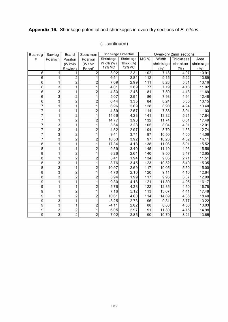
102
Appendix 16. Shrinkage potential and shrinkages in oven-dry sections of E. nitens.
(…continued)
Shrinkage W idth (%) 12%MC
Shrinkage Thick (%) 12%MC
MC % W idth shrinkage
(%)
Thickness shrinkae
(%)
Area shrinkage
(%)6 1 1 2 3.92 2.31 102 7.13 4.07 10.916 1 2 1 6.51 2.81 112 9.15 5.22 13.896 1 2 2 7.09 2.99 111 8.28 5.31 13.166 3 1 1 4.01 2.89 77 7.19 4.13 11.026 3 1 2 4.33 2.48 81 7.59 4.43 11.696 3 2 1 5.07 2.91 86 7.93 4.94 12.486 3 2 2 6.44 3.35 84 8.24 5.35 13.157 1 1 1 6.96 2.69 128 8.90 4.94 13.407 1 1 2 4.89 2.57 114 7.38 3.94 11.037 1 2 1 14.66 4.23 141 13.32 5.21 17.847 1 2 2 14.77 3.93 132 11.74 6.51 17.497 3 1 1 3.54 3.28 105 8.04 4.31 12.017 3 1 2 4.52 2.97 104 8.79 4.33 12.747 3 2 1 9.41 3.71 97 10.50 4.00 14.087 3 2 2 10.53 3.92 97 10.23 4.32 14.118 1 1 1 17.34 4.18 138 11.06 5.01 15.528 1 1 2 9.59 3.40 145 11.19 4.93 15.568 1 2 1 8.26 2.61 140 9.50 3.47 12.658 1 2 2 5.41 1.94 134 9.05 2.71 11.518 3 1 1 8.76 3.45 123 10.52 5.40 15.358 3 1 2 10.97 2.69 117 10.05 5.50 15.008 3 2 1 4.70 2.10 120 9.11 4.10 12.848 3 2 2 3.94 1.99 117 9.95 3.37 12.999 1 1 1 9.30 4.18 121 11.80 4.95 16.179 1 1 2 5.76 4.38 122 12.85 4.50 16.789 1 2 1 7.16 5.12 113 13.67 4.41 17.489 1 2 2 10.61 4.60 114 14.69 4.35 18.409 3 1 1 -3.25 2.73 96 9.81 3.77 13.229 3 1 2 -4.11 2.82 88 8.88 4.56 13.039 3 2 1 6.05 2.97 91 11.30 4.16 14.989 3 2 2 7.02 2.85 90 10.79 3.21 13.65
Shrinkage Potential Oven-dry 2mm sectionsBushlog #
Sawlog Position
Board Positon (W ithin Sawlog)
Specimen Position (Within Board)