Final Report: Conserving our only endemic mammal: habitat associations and

genetic diversity of the maritime shrew, Sorex maritimensis

Researcher: Kimberly Dawe Principle Investigator: Tom Herman

Acadia University September 28, 2005

TABLE OF CONTENTS

ABSTRACT 1

ACKNOWLEDGEMENTS 1

BACKGROUND 2

OBJECTIVES 3

STUDY LOCATIONS AND TRAPPING PROCEDURES 3

PART I: HABITAT ASSOCIATIONS OF THE MARITIME SHREW 4

METHODS 4 HABITAT VARIABLES 4 DATA ANALYSIS 5 RESULTS 5

PART II: GENETIC DIVERSITY AND DIFFERENTIATION 8

METHODS 8 EXTRACTION/PCR/SEQUENCING 8 DATA ANALYSIS 9 RESULTS 10

GENERAL DISCUSSION 19

CONCLUSIONS 20

REFERENCES 20

FINANCIAL REPORT 24

BUDGET SUMMARY 24 DETAILED EXPENDITURE REPORT 25

ABSTRACT The maritime shrew, Sorex maritimensis, was recently elevated to species status, and is thus, endemic and limited in distribution to maritime Canada. Our limited knowledge of the species suggests it is a wetland habitat specialist. These habitats are highly fragmented in Maritime Canada, raising concern for the persistence of this endemic species. To evaluate conservation priorities for the maritime shrew, I modeled habitat variables at spatial and temporal scales using generalized linear mixed models to determine habitat associations and tested for genetic structure between mtDNA sequences using AMOVA and phylogenetic analysis. Habitat models indicate that maritime shrew presence is related to structure and composition variables typical of wetland habitats. Variation in shrew presence was best explained by small-scale habitat variation. Phylogenetic analysis revealed two clades representing Nova Scotia and New Brunswick, with some mixing in the border region. This is suggestive of geographic isolation across the historically flooded isthmus separating the provinces, and more recent gene flow across that wetland. Further population structure was found within New Brunswick. Isolation by distance and barrier influence maritime shrew population genetic structure. Genetic diversity in Nova Scotia is lower than that in New Brunswick and may indicate a historic bottleneck or a selective sweep. Results suggest that contiguous wetland habitats are important for maintaining connectivity and gene flow between populations of the maritime shrew. Conservation efforts should focus on maintaining marsh and wet meadow habitats and monitoring small isolated populations. ACKNOWLEDGEMENTS Funding for this project came from many sources; Acadia University Teaching Fellowships, Nova Scotia Museum Rare Species Grant, IUGB Wildlife Research Award, Margaret McCarthy Research Scholarship, New Brunswick Museum F.M. Christie Research Fellowship in Zoology, Nova Scotia Habitat Conservation Fund, New Brunswick Wildlife Trust Fund, and NSERC. I am very thankful for these contributions. Colin McKinnon of the Canadian Wildlife Service, Eric Tremblay of Kouchibouguac National Park, and Joe Kennedy of the New Brunswick Department of Natural Resources and Energy (Hampton) contributed local expertise and in-kind support to this project. I am grateful for their assistance. I also thank the many landowners for the use of their property and Margaret Wheaton for accommodation and kindness. Many others have made this research possible. Tom Herman and Don Stewart were co-advisers on this project and provided much support and guidance. Soren Bondrup-Neilson, also on my thesis committee, provided advice throughout and Ruth Newell identified my many plant samples. I am sincerely thankful for the hard work of my field and lab assistants Julie Read, Patrick McCamphill, Owen Thompson, and Roxanne Struk. I am also grateful to Phil Taylor and Joe Nocera for statistical help and Sara Good-Avila for analytical advice. Research truly is a collaborative effort.

1/26

BACKGROUND

Nova Scotia supports a disproportionate array of species with ranges disjunct from populations in the rest of North America (Herman and Scott 1992). These include, but are not limited to, Blandings turtle, Emydoidea blandingii (Mockford et al. 2005), southern flying squirrel, Glaucomys volans, rock vole, Microtus chrotorrhinus (Scott and Hebda 2004), numerous Atlantic coastal plain flora (Wisheu et al. 1994), and blue-spotted salamander, Ambystoma laterale (Brownlie 1988). Many of these disjuncts are nationally designated at risk and are attracting increasing attention because of their potential for unique genetic diversity and their vulnerability to rapid environmental change.

The maritime shrew, Sorex maritimensis, considered a part of this assemblage of disjunct species, occurs in Nova Scotia and New Brunswick (Stewart et al. 2002). This species was formerly thought to be a disjunct sub-species of the arctic shrew, Sorex arcticus, whose range extends from the southern Yukon, to the mid western United States and east to Quebec (Kirkland and Schmidt 1996). Recently elevated to species status, the maritime shrew now represents the only mammal endemic to maritime Canada, and only the second endemic to Canada as a whole (the other being the Vancouver marmot, Marmota vancouverensis) (Volobouev and Van Zyll De Jong 1988; Stewart et al. 2002). When species are restricted to, or endemic to, a small range, they have an increased risk of extinction due to both deterministic and stochastic events (Zalba and Nebbia 1999). Endemism is one of many potential measures of species rarity, and rarity, is also an indication of extinction risk (Hartley and Kunin 2003). The maritime shrew is ranked as uncommon or restricted in range (‘S3’ in the provincial ranking system) in both Nova Scotia and New Brunswick (Atlantic Canada Conservation Data Center, 2005). Both of these issues increase concern for the persistence of the maritime shrew.

This species was ranked among the most susceptible to climate change in Nova Scotia, based largely on an apparent affinity for wetland habitats (Herman and Scott 1992). Climate change predictions suggest increases in global temperatures of 2-5 °C by 2050, rises in sea level by more than 80 cm, increases in precipitation, evapotranspiration, and runoff, as well as decreases in summer soil moisture (Michener et al. 1997). Wetlands are sensitive to water level shifts and human induced changes through development and land use practices further increase the vulnerability of these ecosystems and the species within them to climate change effects (Mortsch 1998).

While global trends show evidence of climate induced responses, the local processes of habitat loss, fragmentation, and land use practices drive the majority of current biological changes and influence species’ abilities to respond to changing climate (Parmesan and Yohe 2003). For example, habitat loss isolated two populations of checkerspot butterfly, a species with limited dispersal ability. Individuals were unable to migrate in response to temperature and precipitation shifts and subsequently both populations went extinct (McLaughlin et al. 2002).

Shrews also have limited dispersal abilities (Peltonen and Hanski 1991) and thus, may be particularly susceptible to fragmentation effects (Goheen et al. 2003). Landscape connectivity is a measure of a species’ ability to move within its landscape. It is the combined effect of the distance between patches, the configuration of the landscape matrix between those patches and the dispersal abilities of particular species (Taylor

2/26

2000). In the absence of species-specific information, a direct assessment of landscape connectivity may not be possible; however, gaining an understanding of what constitutes a ‘habitat patch’ for the species of interest is a critical step toward that end.

Also, dispersal success provides an index of connectivity and, although molecular markers contain information on historic processes, they have also proved to be effective in making inferences about dispersal movements and thus are useful for estimating connectivity (Bohonak 1999; Branch et al. 2003). Genetic studies measure dispersal leading to successful reproduction, or gene flow, which is averaged over generations and is less influenced by current population size than are direct measures of dispersal success (Schumaker 1996; Bohonak 1999; Mech and Hallett 2001). In rare or less studied species, such as the maritime shrew, this approach allows for timely conservation assessment when basic information required for direct analysis is lacking (Doak and Mills 1994).

Here we investigate the habitat associations and population genetic structure of the maritime shrew to better equip managers with the information necessary to ensure the persistence of this endemic mammal. OBJECTIVES The objectives of the study were:

• To determine the habitat associations of the maritime shrew at several spatial scales.

• To determine the genetic structure within and between locally and regionally defined maritime shrew populations.

• To determine how these factors influence the risks to the species’ persistence. STUDY LOCATIONS AND TRAPPING PROCEDURES

Trapping occurred in 14 locations during the progress of this project (Figure 1). Maritime shrews were captured at all but 5 of these locations, which had undergone sampling prior to the period supported by the Fund. Of the remaining 9 locations, all yielded samples for genetics analysis, and 6 underwent intensive pitfall trapping and habitat sampling. Pitfall traps, 750 ml yogurt containers, were set flush with the ground, filled with 3 inches of water, and checked daily. This trap method (Churchfield and Sheftel 1994) or variations of it (Ryan 1986; Bellocq et al. 1992; Blackburn and Andrews 1992; Churchfield et al. 1997; McCay and Storm 1997; Churchfield et al. 1999; Diaz de Pascual and De Ascencao 2000) has been used extensively for trapping shrews. Maximum use was made of samples in this study. In addition to collecting habitat data for each capture, tissue samples were collected for genetic analysis and morphometric, age, and sex data were collected for future analysis. All specimens were deposited in provincial museums.

During August 2003 wet pitfall traps were set in a systematic grid design such that one to four sites, depending on the size of the available area, were sampled in each of the six locations. Sites contained 36-54 traps set in 3 x 3 grids (9 traps) with 10 m

3/26

between traps and 50 m between grids. The first trap in a site was placed, non-randomly, in marsh or old-field habitat such that a minimum of 36 traps could be placed in the site. Traps remained in place for three nights. If water in the traps appeared to be more than 3 inches deep or if sticks had fallen into the traps, they were classified as having lower efficacy. These traps were not excluded from the analysis because captures still occurred.

Figure 1: Location map for preliminary and study sites. Letters indicate sites without maritime shrews; numbers indicate sites with captures. Sites are (A) Belleisle and Queen Anne Marsh, (B) Waterloo Lake, (C) Cornwallis River, (D) Wolfville, (E) Falmouth, (1) Stanley, (2) South Branch, (3) Oxford, (4) Wallace Bay, (5) Cape Jourimain, (6) Tantramarre Marsh, (7) Shepody, (8) Hampton Marsh, and (9) Kouchibouguac National Park. Sites 4, 5, and 7 were used only for genetics analysis. PART I: HABITAT ASSOCIATIONS OF THE MARITIME SHREW METHODS Habitat variables

Weather and Moon Phase data were obtained from Environment Canada’s “Climate Data On-line” (Meteorological Society of Canada 2002), and the United States Naval Observatory (Astronomical Applications Department 2003), respectively. Habitat variables were collected at both trap and grid scales.

Vegetation height above each trap was recorded with a meter stick prior to digging the pitfalls to reduce trampling bias. Insects were collected from pitfalls at the end of each trapping session, placed in 70 – 100% ethanol, and identified to Order. Biomass was obtained by assuming a 3:1 ratio between biomass and length and arthropod biomass was pooled to obtain a single measure of prey abundance.

The percent cover of trees, open water, and roads within each grid was estimated. Pools, flooded marshes, and/or standing bodies of water signified open ‘water’ in a grid and persistent trails, pathways, or hard packed roads characterized ‘roads’. Soil was ranked as dry, wet, or very wet. Estimates of distance to water and roads were made by sight from a grid to the nearest body of water and hard packed road, respectively.

4/26

Vegetation association was represented by the plant species found most frequently to be in the top three most abundant (by % cover) plant species in a grid.

Data Analysis

Because there were no positive capture sites south of Stanley, data from these locations may have been outside of the species’ current distribution and thus were not included in the analysis. I tested for spatial autocorrelation of maritime shrew presence at the trap and grid scales using correlograms in the software package Passage (Rosenberg 2001). The relationship between maritime shrew presence and measured habitat characteristics was modeled using the generalized linear model (glm) framework under a binomial distribution in the R program (2004).

Best models were selected according to AIC (Akaike 1974) and ranked using AIC weights (Wagenmakers and Farrell 2004). Models having an evidence ratio < 2 were considered to be equally likely (Burnham and Anderson 2002). For all models, correlation between weather variables was tested using Generalized Spearman Rank Correlation. Where variables were correlated (r ≥ 0.7), each variable was individually tested in the model. Only the variable producing the model with the lowest AIC was included in the analysis.

Parameters were removed one at a time from a maximum model containing all habitat and uncorrelated weather variables. At each step, the parameter estimate with the largest p value was removed from the model. If the resulting model AIC was higher than the previous model, that parameter was re-inserted, otherwise it remained out of the model and the next parameter was chosen for elimination. This continued until the model with the lowest AIC was attained.

Spatially structured sampling can induce spurious results if not accounted for in models (Dalthorp 2004), thus, the top glm’s were incorporated into generalized linear mixed effects models using penalized quasi-likelihood (glmmPQL) where grid was nested in site, which was nested in location. Because there is no singular accepted method for selecting best models in the glmm framework and there are still uncertainties in aspects of glmm theory (Madden 2002), assessing the models in glm form allowed for a less subjective assessment of top models and subsequent calculation of parameter estimates and variance components in the glmmPQL framework.

Model fit was evaluated using Nagelkerke’s pseudo-R2 (Nagelkerke 1991) and area under a receiver operating characteristic curve (AUC) (Hanley and McNeil 1982), implemented in the R program under the Design package (R Development Core Team, 2004). The receiver operating characteristic curve is constructed by the probability of obtaining a false positive versus the probability of obtaining a true positive and AUC provides an estimate of how often maritime shrew presence is correctly predicted by a given model. The AUC values range from 0.5 to 1.0 with 0.5 having no discrimination ability and values > 0.7 having acceptable discrimination (Hanley and McNeil 1982; Betts et al. 2005). RESULTS

A total of 252 small mammals, 139 of which were S. maritimensis, were captured using 821 traps over 2451 trap nights. The maritime shrew comprised 55% of all small

5/26

mammals captured. Catch per unit effort (cpue) for the target species varied by location and by year (Table 1.1). Although Rudd (1955) found that males occurred in traps more frequently, captures here consisted of 45.3% males, and 48.9% female (5.8% could not be determined). Descriptive statistics for all predictive variables can be found in Table 1.2. There was no spatial autocorrelation detected in maritime shrew presence and thus raw data was used for all models.

Table 1.1: Trap success across sampling locations. Catch per unit effort (cpue) is measured as the number of maritime shrews caught/trap night. UTM = Universal Transverse Mercator Coordinate System; TN = Trap nights.

Location County/Province UTMs Date TN Cpue Tantramarre Marsh Westmorland County,

NB 0398856 5084353

3 Aug, 2003 526 0.091

Kouchibouguac National Park

Kent County, NB 0354595 5198994

8 Aug, 2003 400 0.043

Hampton Kings County, NB 0279828 5046050

13 Aug, 2003 277 0.069

South Branch Colchester County, NS 0494682 5003062

18 Aug, 2003 253 0.028

Stanley Hants County, NS 0426366 4992740

23 Aug, 2003 243 0.016

Oxford Cumberland County, NS 0431600 5063795

27 Aug, 2003 135 0.089

6/26

Table 1.2: Descriptive data for habitat variables included in the maximum model for spatial analyses. Counts are included for each level of categorical variables. All weather data were averaged over the trap period. Units and model codes are in brackets after the variable description; (Standard deviation).

Presence Absence Variable Mean Mean Location Average moon illuminated (%) (meanmoon) 0.56

(0.29) 0.57

(0.32) Min temperature (°C) (min) 13.95

(3.71) 13.33 (3.89)

cloud (% of hours) (cloud) 23.48 (2.75)

21.65 (3.57)

rain, drizzle, or fog (% of hours) (rdf) 21.23 (14.75)

16.31 (13.94)

Grid % cover of trees (t) 15.34

(23.66) 26.12

(33.00) % cover of open water (w) 1.25

(5.11) 0.96

(4.40) % cover of trails, paths or roads (r) 2.53

(13.63) 2.79

(14.28) Distance to body of water (m) (dtw) 52.12

(69.84) 94.43

(105.47) Distance to hard packed road (m) (dtr) 93.30

(113.01) 99.80

(95.20) Calamagrostis canadensis (calcan) present 37 151

absent 42 405 Soil (soil) dry 20 267

wet 42 234 Vwet 17 55 Cover (cover) yes 5 113 no 74 443 Trap Proportion of trap period when trap was 100% effective (eff)

0.98 (0.09)

0.95 (0.18)

Vegetation height (cm) (vh) 68.82 (27.85)

48.04 (37.73)

Prey abundance (prey) 186.97 (600.48)

237.33 (1000.50)

There were two top models (AIC evidence ratio < 2) (Table 1.3). Approximately

20% of the variation in maritime shrew presence was explained by the habitat variables, with a predictive accuracy of 78%.

Table 1.3: Top generalized linear mixed effects models (using penalized quasi-likelihood) according to AIC (Akaike 1974) and evidence ratios for generalized linear models. AUC is the area under a receiver operator characteristics curve (Hanley and McNeil 1982). Rank Scale Model Evidence Ratio Pseudo-R^2 AUC

1 Spatial sma~meanmoon+cloud+eff+vh+t+r+dtr+calcan | loc/site/grid 1.0000 0.204 0.7832 Spatial sma~meanmoon+cloud+eff+vh+t+r+calcan |loc/site/grid 1.3034 0.197 0.775

Weather, structure and composition variables were retained in all models (Table

1.4). Average moon illumination and cloud cover had a significant, positive relationship

7/26

with shrew presence. Vegetation height was higher and Calamagrostis canadensis was likely to be present where maritime shrews were present. Percent cover of trees had a negative relationship with maritime shrew presence. Higher percent cover of trails and pathways within a grid and smaller distances to hard packed roads were also an important predictors of shrew presence, although the relationships were not significant. Shrews were only captured in traps with 67% efficacy or higher.

Table 1.4: Generalized linear mixed effects model (using penalized quasi-likelihood) of the relationship between maritime shrew presence and habitat characteristics in six locations across Maritime Canada. Parameter estimate SE p y-int -12.783176 1.9651218 0.0000meanmoon 1.380832 0.5822201 0.0495cloud 0.324305 0.061301 0.0011eff 1.896937 1.0363392 0.0677vh 0.014089 0.0039348 0.0004t -0.013321 0.0062784 0.0387r 0.022647 0.0115365 0.0550dtr -0.002051 0.001438 0.1597calcan 1.031211 0.3358896 0.0034

The variance components for the spatial model indicate that the trap and grid scales explain the most variation in maritime shrew presence (Table 1.5).

Table 1.5: Variance components and standard deviation from group means for grouping at various spatial scales. Scale variance sd location 0.000921 0.030355 site 0.131256 0.362293 grid 0.394875 0.628391 residuals 0.685666 0.828050 PART II: GENETIC DIVERSITY AND DIFFERENTIATION METHODS Extraction/PCR/sequencing

Shrews were frozen within 48 hours of capture. Necropsies were conducted on thawed shrews and tissues were preserved in an -80°C freezer in 1.5 ml microtubes. Shrew remains were re-frozen for later preparation at local museums.

Total DNA was isolated from approximately 10 mg of kidney tissue using a Qiagen Dneasy Tissue Kit. The optional RNase treatment was not performed. The concentration of total DNA was estimated using a 1 in 10 dilution in an Ultraspec 3100 pro UV-visible spectrophotometer (Pharmacia). Total DNA eluted in Qiagen’s EB buffer was stored at -4°C and working dilutions of 25 ng/ul (in ddH2O) were stored at -20°C.

8/26

The control region of the mitochondrial DNA genome was amplified by polymerase chain reaction in a PTC-100 or PTC-200 Peltier Thermalcycler (MJ research). Reactions (50 ul total volume) consisted of 2 ul of 25ng/ul template, 27.2 ul of ddH2O, 2.6 ul of 50 mM MgCl2, 5.0 ul of 10 x reaction buffer, 5.0 ul of 8 mM dNTPs, 0.2 ul of 5 U/ul Platinum™ Taq (Invitrogen), and 4.0 ul of each primer (10 pmol/ul). Primers used were tRNA pro, 5’ CCCCACCATCAGCACCCAAAGC 3’ and CSB-F, 5’ AGCGGGTTGCTGGTTTCACG 3’. The PCR cycling program began at 94°C for 3 minutes followed by 40 cycles of: 94°C for 30 sec, 45°C for 45 seconds, and 72°C for 60 seconds. This program ended with an additional 5 minutes at 72°C. PCR product was electrophoresed in a 1% agarose gel in 1xTAE buffer using 20 ul of template and 2 ul of tracking dye (Blucose) per well. Two wells were run for each sample. Gels were visualized on a BIO-RAD Gel Doc 2000 using the preparative setting to protect the DNA from degradation. Bands were cut out and extracted using a Qiagen Gel Extraction Kit. Because the fragment amplified was ~800 bp long, isopropanol was not added in optional step five of the gel extraction protocol for use with a microcentrifuge. All traces of agarose were removed using the optional QG buffer wash. DNA was eluted in 30 ul of ddH2O rather than the elution buffer provided in the kit. The concentration of cleaned DNA was obtained using a 1:10 dilution factor in the UV/visible light spectrophotometer. Cleaned DNA was stored at -20°C. All hot water bath steps for the Qiagen kits were carried out in an Isotemp 202s water bath. An IEC Micromax or an Eppendorf 5804R microcentrifuge was used at 13000 rpm for all spins. Sequencing was conducted from the tRNApro, or 5’, end of the D-loop fragment to obtain data for the hypervariable region. In the control region of shrews, the hypervariable region has the highest rate of mutation making it most suitable for intraspecific analyses (Stewart and Baker 1994). DNA sequencing was initially performed at Florida State University on an Applied Biosystems 3100 Genetic Analyzer. Sequencing was also conducted at the Acadia University Sequencing Facility on a Base Station 5 (MJ Research). Data Analysis

Sequencing chromatograms were examined in Chromas (McCarthy 1996) to identify and correct any mis-called bases from the sequencing process. Sequences were then manually aligned, without ambiguities, using Se-al 2.0 (Rambaut 1996). Sorex arcticus (the sister species to S. maritimensis) sequences were automatically aligned using Clustal W (Chenna et al. 2003) then incorporated manually into the main data set as an outgroup. These were excluded from the analysis however, because they proved to be too distant from Sorex maritimensis to be confidently aligned, particularly for the hypervariable segment of the control region.

Haplotypes were identified using Collapse (Posada version 1.2). Arlequin (Schneider et al. 2000) was used for all analyses except where specified. Haplotype diversity, nucleotide diversity, and population parameter (θ) estimates were calculated for the entire Maritimes, for each province and for each local population. Following Nei and Kumar (2000), I used the proportion of pairwise differences for all distance calculations. When pairwise differences are less that 0.10, or 10% divergence, more complicated

9/26

distance methods have little effect on distance estimates and have larger variances associated with the estimates (Nei and Kumar 2000).

The phylogenetic relationship of samples was investigated using maximum parsimony with 1000 bootstrap replicates. Gaps were treated as a fifth state. Maximum parsimony was performed using PAUP (Swofford 2003). A neighbour joining tree was generated using the MEGA package (Kumar et al. 2001). Missing data and gaps were deleted in pairwise comparisons. The robustness of the resulting topology was tested using 1000 bootstrap replicates. A statistical parsimony network was generated using the TCS software program (Clement et al. 2000). The network calculates the 95% confidence set of connections, allowing for non-bifurcating associations and does not assume extinction of ancestral haplotypes (Clement et al. 2000). Confidence in the network also increases when the difference between individuals is minimal as is the case with this intraspecific data (Posada and Crandall 2001). Loops or arbitrary connections in the network were resolved, when possible, according to Pfenninger and Posada’s (2002) frequency, topological, and geographic criteria.

Analysis of Molecular Variance (AMOVA) was used to test population genetic structure at regional and local scales (Excoffier et al. 1992). Modified F statistics (φ statistics) were calculated for each scale of analysis and permutation tests were employed to test whether the observed φ statistics were significantly different from 0 (Excoffier et al. 1992). The modification of Wright’s (1965) FST is calculated using θπ estimates instead of heterozygosity, allowing for analysis of mtDNA data. Distance between all pairwise combinations of populations was calculated using φST and corrected mean pairwise nucleotide difference, Da, was also calculated.

To test for isolation by distance, φST was regressed against pairwise geographic distance between local populations in the R statistical package (R Development Core Team, 2004). A Mantel test was run in TFPGA (Tools For Population Genetic Analyses) (Miller 1997) to test for significant correlation between both matrices. The geographic distance between locations in Nova Scotia and New Brunswick respectively, was calculated as the additive distance from each of the local populations to the center of the narrowest point along the Isthmus of Chignecto. Intra-province distances were calculated as straight-line distance.

Tajima’s D (Tajima 1989) was calculated across the Maritimes, across regions, and across local populations, respectively, to test for population growth.

RESULTS

A total of 68 maritime shrew sequences, 292 bp long was obtained. This segment included 137 base pairs of the unique flanking region and two 79 bp tandem repeats. The unique flanking region is slightly longer than 137 bp in this species; however, the sequence was trimmed at both ends to minimize missing data. The nucleotide composition was T: 31.8%, C: 21.3%, A: 39.7%, and G: 7.2%.

There were 31 unique haplotypes identified (Table 2.1) and the maximum p-distance between haplotypes was 0.0383. Of 22 variable sites, 19 were parsimony informative. There were 18 transitions, 0 transversions, and 4 indels (ie., insertions or deletions). Two main clades were evident in the neighbour joining and maximum parsimony trees: a New Brunswick clade and a predominantly Nova Scotia clade (Fig.

10/26

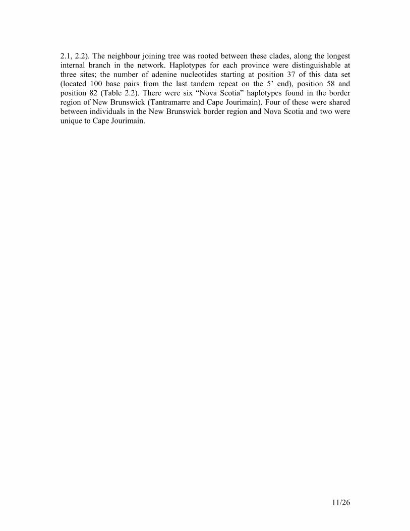
2.1, 2.2). The neighbour joining tree was rooted between these clades, along the longest internal branch in the network. Haplotypes for each province were distinguishable at three sites; the number of adenine nucleotides starting at position 37 of this data set (located 100 base pairs from the last tandem repeat on the 5’ end), position 58 and position 82 (Table 2.2). There were six “Nova Scotia” haplotypes found in the border region of New Brunswick (Tantramarre and Cape Jourimain). Four of these were shared between individuals in the New Brunswick border region and Nova Scotia and two were unique to Cape Jourimain.

11/26

Table 2.1: Haplotype numbers (Hap) and variable sites for a 292 bp long segment of the control region from 68 maritime shrews. Sample numbers indicate the collector, catalogue number and abbreviated sampling location; Stanley (stan), Oxford (oxf), South Branch (sb), and Wallace Bay (wb), Nova Scotia, and Tantramarre (tant), Cape Jourmain (cj), Hampton (hamp), Kouchibouguac (kouch), Shepody (shep), and Portabello Creek (pc), New Brunswick. There are 22 variable sites and 12 sites with missing data. Hap Samples Position of Variable Sites and Missing Data

0000000000000000001111111122222222 0000000004444567891345699913357788 1234567893456891253319034817811239

1 kd278stan, kd285stan AGCCAAAAC----TGCGCCCCTTTCCTTTCTCCT 2 kd279stan, kd290oxf, kd295oxf, kd339oxf,

kd345oxf, kd107tant AGCCAAAAC----TACGCCTCTTTCCTTTCTCCT

3 kd287sb ????????C----TACGCTTCTTTTCTTTCTTCT 4 kd288sb ????????C----TACGCCCCTTTCCTTTCTCCT 5 kd298sb, kd299sb, kd300sb, kd293oxf,

kd294oxf, kd427wb, kd429wb, kd254tant, kd132tant

AGCCAAAAC----TACGCCCCTTTCCTTTCTCCT

6 kd306sb ?????????----TACGCCCCTTTCCTTTCTCCT 7 kd297oxf AGCCAAAAC----TACGCCCCTTTCNTTTCTCCT 8 kd344oxf, kd428wb, kd332tant AGCCAAAAC----TACGCCCCTTTCCCTTCTCCT 9 kd346oxf AGCCAAAAC----TACGCCCCTTTCCTTTTTCTT

10 kd430cj AGCCAAAACAA--CACACCTCTTTTCTTTCTTCT 11 kd431cj, kd432cj, kd434cj, kd437cj AGCCAAAAC----TACGCTTCTTCCCTTTCCCCT 12 kd433cj AGCCAAAACAA--CACACCTCTTTTCTTTCTCCT 13 kd435cj, kd436cj, kd422pc AGCCAAAACAAA-CACACCTCTTTTCTTTCTTCT 14 kd438cj AGCCAAAAC----TACGCTTCTTCCCTTTCTCCT 15 kd259tant AGTCAAAACAAAACANACCTCTTTCCTTTCTTCT 16 kd136tant, kd256tant AGCCAAAACAAAACACACCTCTTTTCTTTCTTCT 17 kd257tant AGCCAAAACAAAACACACCTCTTCCCTTTCCCCT 18 kd131tant AGCCAAAAC----TACGCCCCTTTCCCTTCTCCC 19 kd333tant AGCCAAAACAAA-CACACCTCTTTTCTTTCTCCT 20 kd134tant, kd309hamp, kd313hamp,

kd315hamp, kd317hamp, kd420kouch, kd312hamp, kd413kouch

AGCCAAAACAAA-CACACCTCTTTCCTTTCTCCT

21 kd135tant, kd414kouch AGCCAAAACAAAACACACCTCTTTCCTTTCTCCT 22 kd423shep, kd425shep AGCCAAAACA---CACACCTCTTTTCTTTCTTCT 23 kd424shep AGCCAAAACAAA-CACACCTCCTTCCTTTCTCCT 24 kd426shep, kd316hamp AGCCAAAACAAA-CACACCTCCTTCCTCTCTCCT 25 kd308hamp AGCCAAAACAAA-CACACCTCTTTCCTCTCTCCT 26 kd310hamp, kd320hamp, kd330hamp,

kd421kouch AGCCAAAACAA—CACACCTCTTTCCTTTCTCCT

27 kd319hamp, kd376kouch AGCCAAAACAAA-CACANCTNTTTCCTTTCTCCT 28 kd304hamp ?????????AA--CACACCTCTTTCCTTTCTCCT 29 kd389kouch, kd418kouch AGCCAAAACAA--CACACCTCTCTCCTTCCTCCT 30 kd404kouch AGCCAAAACAA--CACACCTCTTTCCTCTCTCCT 31 kd407kouch AGTCAAAACAA--CACACCTCTTTCCTTTCTCCT

12/26

2324

2530

2920262721

2815

311219

16131022

1711

1403

0208

1809

0105070406

67

64

615031

32

28

66

35

75

534554

51

52

41

33

48

45

45

42

27

24

32

25

11

25

0.002

Shepody (1)Hampton (2)Shepody (1) Kouchibouguac (1)

Tantramarre (1), Hampton (5), Kouchibouguac (2)Hampton (3), Kouchibouguac (1)Hampton (1), Kouchibouguac (1)Tantramarre (1), Kouchibouguac (1)Hampton (1)

Kouchibouguac (2)

Tantramarre (1)Kouchibouguac (1)Cape Jourimain (1)Tantramarre (1)Tantramarre (2)Cape Jourimain (2), Portabello Creek (1)Cape Jourimain (1)Shepody (2)Tantramarre (1)Cape Jourimain (4)Cape Jourimain (1)South Branch (1)Stanley (1), Oxford (4), Tantramarre (1)Oxford (1), Wallace Bay (1), Tantramarre (1)Tantramarre (1)Oxford (1)Stanley (2)South Branch (3), Oxford (2), Wallace Bay (2), Tantramarre (2)Oxford (1)South Branch (1)South Branch (1)

New

Brunsw

ickN

ova Scotia +

Figure 2.1: Neighbour-joining tree calculated using p-distances based on 292 bp of control region sequence. Numbers to the right of the branches refer to haplotype designations (Table 2.1). Numbers to the left refer to bootstrap support for clades based on 1000 bootstrap replications.

13/26

10 Cape Jourimain (1)12 Cape Jourimain (1)13 Cape Jourimain (2), Portabello Creek (1)15 Tantramarre (1) 16 Tantramarre (2)17 Tantramarre (1)19 Tantramarre (1)20 Tantramarre (1), Hampton (5), Kouchibouguac (2)21 Tantramarre (1), Kouchibouguac (1)22 Shepody (2)23 Shepody (1)24 Hampton (2)25 Shepody (1)26 Hampton (3), Kouchibouguac (1)27 Hampton (1), Kouchibouguac (1)28 Hampton (1)29 Kouchibouguac (2)30 Kouchibouguac (1)31 Kouchibouguac (1)

81

02 Stanley (1), Oxford (4), Tantramarre (1)03 South Branch (1)11 Cape Jourimain (4)14 Cape Jourimain (1)04 South Branch (1)05 South Branch (3), Oxford (2), Wallace Bay (2), Tantramarre (2)06 South Branch (1)07 Oxford (1)08 Oxford (1), Wallace Bay (1), Tantramarre (1)18 Tantramarre ( 1)09 Oxford (1)01 Stanley (2)

68

65

63

New

Brunsw

ickN

ova Scotia +

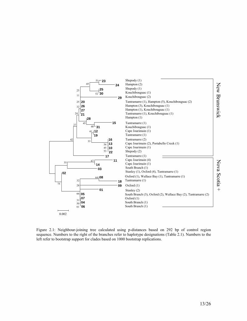
Figure 2.2: Maximum parsimony tree calculated using p-distances based on 292 bp of control region sequence. Numbers to the right of the branches refer to haplotype designations (Table 2.1). Numbers to the left refer to bootstrap support for clades based on 1000 bootstrap replications. Table 2.2: Major haplotype differences between clades compared with the sister species. Nucleotide position Group 37 - 47 (A array) 58 82 Nova Scotia 6 T G New Brunswick 7-10 C A Sorex arcticus 5 (array at bp 26) gap A

Haplotype and nucleotide diversity was lower in Nova Scotia than in New Brunswick or the Maritimes as a whole (Table 2.3). When calculated by clade, thus incorporating all “Nova Scotia” haplotypes together, the nucleotide diversity in Nova Scotia and New Brunswick was nearly the same. Haplotype diversity remained higher in New Brunswick, however. Geographic distribution of haplotypes was evident in New Brunswick with a Hampton/Kouchibouguac clade and a Tantramarre/Cape Jourimain clade, although Tantramarre haplotypes tended to be distributed throughout the trees. Bootstrap values were generally low (<50%) for the phylogenetic trees. This may be due to violation of the assumption of identical rates of evolution across the fragment analyzed as well as its relatively small size (Page and Holmes 1998).

14/26

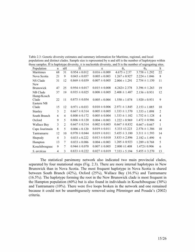
Table 2.3: Genetic diversity estimates and summary information for Maritime, regional, and local populations and distinct clades. Sample size is represented by n and nH is the number of haplotypes within those samples. Ĥ is haplotype diversity, π is nucleotide diversity, and S is the number of segregating sites.

Population n nH Ĥ π θπ θS S Maritimes 68 31 0.954 ± 0.012 0.016 ± 0.009 4.675 ± 2.57 3.758 ± 1.292 22 Nova Scotia 21 9 0.843 ± 0.057 0.005 ± 0.003 1.267 ± 0.927 2.224 ± 1.046 8 NS Clade 31 12 0.869 ± 0.039 0.007 ± 0.005 2.004 ± 1.291 2.754 ± 1.150 11 New Brunswick 47 25 0.954 ± 0.017 0.015 ± 0.008 4.242± 2.378 3.396 ± 1.263 19 NB Clade 37 19 0.935 ± 0.025 0.008 ± 0.005 2.408 ± 1.487 2.156 ± 0.931 12 Hamp/Kouch Clade 22 11 0.875 ± 0.054 0.005 ± 0.004 1.550 ± 1.074 1.920 ± 0.931 9 Eastern NB Clade 15 12 0.971 ± 0.033 0.010 ± 0.006 2.971 ± 1.845 2.153 ± 1.085 10 Stanley 3 2 0.667 ± 0.314 0.005 ± 0.005 1.333 ± 1.370 1.333 ± 1.098 2 South Branch 6 4 0.800 ± 0.172 0.005 ± 0.004 1.333 ± 1.102 1.752 ± 1.128 4 Oxford 9 5 0.806 ± 0.120 0.004 ± 0.003 1.222 ± 0.969 1.472 ± 0.906 4 Wallace Bay 3 2 0.667 ± 0.314 0.002 ± 0.003 0.667 ± 0.832 0.667 ± 0.667 1 Cape Jourimain 8 5 0.806 ± 0.120 0.019 ± 0.011 5.333 ±3.223 2.576 ± 1.386 10 Tantramarre 12 10 0.970 ± 0.044 0.019 ± 0.011 5.455 ± 3.180 3.311 ± 1.593 14 Shepody 4 3 0.833 ± 0.222 0.013 ± 0.010 3.833 ± 2.896 2.182 ± 1.490 6 Hampton 13 7 0.833 ± 0.086 0.004 ± 0.003 1.205 ± 0.923 1.289 ± 0.768 5 Kouchibouguac 9 7 0.944 ± 0.070 0.007 ± 0.005 2.000 ±1.408 1.472± 0.906 6 S. arcticus 4 3 0.833 ± 0.222 0.027 ± 0.019 7.333 ± 5.194 5.455 ± 3.270 13

The statistical parsimony network also indicated two main provincial clades,

separated by four mutational steps (Fig. 2.3). There are more internal haplotypes in New Brunswick than in Nova Scotia. The most frequent haplotype in Nova Scotia is shared between South Branch (42%), Oxford (25%), Wallace Bay (16.5%) and Tantramarre (16.5%). The haplotype forming the root in the New Brunswick clade is most frequent in the Hampton population (60%) but is also found in individuals in Kouchibouguac (30%) and Tantramarre (10%). There were five loops broken in the network and one remained because it could not be unambiguously removed using Pfenninger and Posada’s (2002) criteria.

15/26

08 (NS+)

18 (NB)

04, 05, 06, 07 (NS+)

01 (NS)02 (NS+)

09 (NS)

14 (NB)

11 (NB)03 (NS)

22 (NB)

10 (NB)

12 (NB)13 (NB)

16 (NB)19 (NB)

20, 27 (NB)

25 (NB)23 (NB)21 (NB)

24 (NB)

15 (NB)17 (NB)

26, 28 (NB)

29 (NB)

30 (NB) 31 (NB)

KouchibouguacKouchibouguac/HamptonHamptonTantramarreTantramarre/Hampton/KouchibouguacTantramarre/KouchibouguacShepodyCape JourimainCape Jourimain/Portabello CreekSouth BranchStanleyStanley/Oxford/TantramarreOxfordOxford/Wallace Bay/TantramarreSouth Branch/Oxford/Wallace Bay/Tantramarre

LEGEND

Figure 2.3: Statistical parsimony network for the Nova Scotia and New Brunswick haplotypes, calculated using the TCS algorithm (Clement et al. 2000).

The AMOVA indicates that the provinces are significantly differentiated from each other (Table 2.4). All but three interprovincial φST comparisons are significantly different and in New Brunswick, Hampton and Kouchibouguac are differentiated from all populations but each other (Table 2.5). The mean geographic distance between populations in New Brunswick is 106.4 ± 48.0 km, in Nova Scotia it is 69.8 ± 23.3 km, and between provinces it is 141.1 ± 64.9 km. When intraprovincial variation is removed, the average pairwise distance between the provinces is 3.1%. The within province corrected distances were low and between province distances ranged from 1.8% to 5.5% (Table 2.6).

16/26

Table 2.4: Analysis of molecular variance for two hypothesized scales of genetic structure. Scale d.f. Sum of

Squares Variance Components

Percentage of Variation

φ-Statistics Significance

Regional Among populations 1 46.362 1.53951 47.96 Within Populations 66 110.252 1.67049 52.04 φST = 0.4796 p<0.0001 Local Among groups 1 46.362 1.45645 45.43 φCT = 0.4543 p<0.0001 Among populations within groups

8 27.678

0.34974 10.91 φSC = 0.1999 p<0.0001

Within Populations 58 82.575 1.39957 43.66 φST = 0.5634 p<0.0001 Table 2.5: Pairwise φST estimates of molecular variance for local scale comparisons.

Location 1 2 3 4 5 6 7 8 1. Stanley 0.0000 2. South Branch 0.1369 0.0000 3. Oxford 0.1487 0.0114 0.0000 4. Wallace Bay 0.2500 -0.0671 0.0217 0.0000 5. Cape Jourimain 0.2892 0.3168*** 0.3723*** 0.3227* 0.0000 6. Tantramarre 0.2500 0.2838* 0.3225* 0.2433 0.1169 0.0000 7. Shepody 0.6069* 0.6522*** 0.6902*** 0.6456*** 0.2057 0.0828 0.0000 8. Hampton 0.8083*** 0.8033*** 0.7968*** 0.8272*** 0.4387*** 0.2119*** 0.2413* 0.0000 9. Kouchibouguac 0.7203*** 0.7331*** 0.7364*** 0.7448*** 0.3681** 0.1692* 0.2174* 0.0335 * p < 0.05, ** p < 0.01, *** p < 0.001 Table 2.6: Corrected average pairwise nucleotide differences between populations.

Location 1 2 3 4 5 6 7 8 1. Stanley 0.0000 2. South Branch 0.2146 0.0000 3. Oxford 0.2037 0.0109 0.0000 4. Wallace Bay 0.3333 -0.0077 0.0926 0.0000 5. Cape Jourimain 2.3333 1.8812 1.9444 2.6667 0.0000 6. Tantramarre 2.1616 1.8345 1.8098 2.1616 0.7172 0.0000 7. Shepody 4.5000 4.1590 4.1111 4.8333 1.3889 0.6061 0.0000 8. Hampton 5.1410 5.0886 4.7521 5.4744 2.1581 0.8561 0.3077 0.00009. Kouchibouguac 4.8889 4.8257 4.5000 5.2222 2.1358 0.8653 0.5556 0.0385

A linear relationship was seen between φST and geographic distance (r=0.5818, p = 0.002, r2= 0.4763, F1,34=32.83 on 1 and 34 df) (Fig. 2.4). However, the φST values were disproportionately higher for interprovincial population distances indicating a barrier to movement between the provinces. Between-province comparisons with Cape Jourimain and Tantramarre (the border region) do not have equally inflated φST values, however.

17/26

0 50 100 150 200 250

0.0

0.2

0.4

0.6

0.8

distance (km)

FST

0 50 100 150 200 250

0.0

0.2

0.4

0.6

0.8

distance (km)

FST

0 50 100 150 200 250

0.0

0.2

0.4

0.6

0.8

distance (km)

FST

0 50 100 150 200 250

0.0

0.2

0.4

0.6

0.8

distance (km)

FST

NBNSNS-BorderNS-NB (main)

Figure 2.4: Genetic and geographic distance comparison to test isolation by distance. NB is New Brunswick, NS is Nova Scotia. The border region consists of Tantramarre and Cape Jourimain and NB (main) consists of all New Brunswick populations other than the border region.

Neither population had a significant probability of having a Tajima’s D value lower (more negative) than a selectively neutral simulated population at equilibrium, although there was a consistent negative trend across all populations (Table 2.7).

18/26

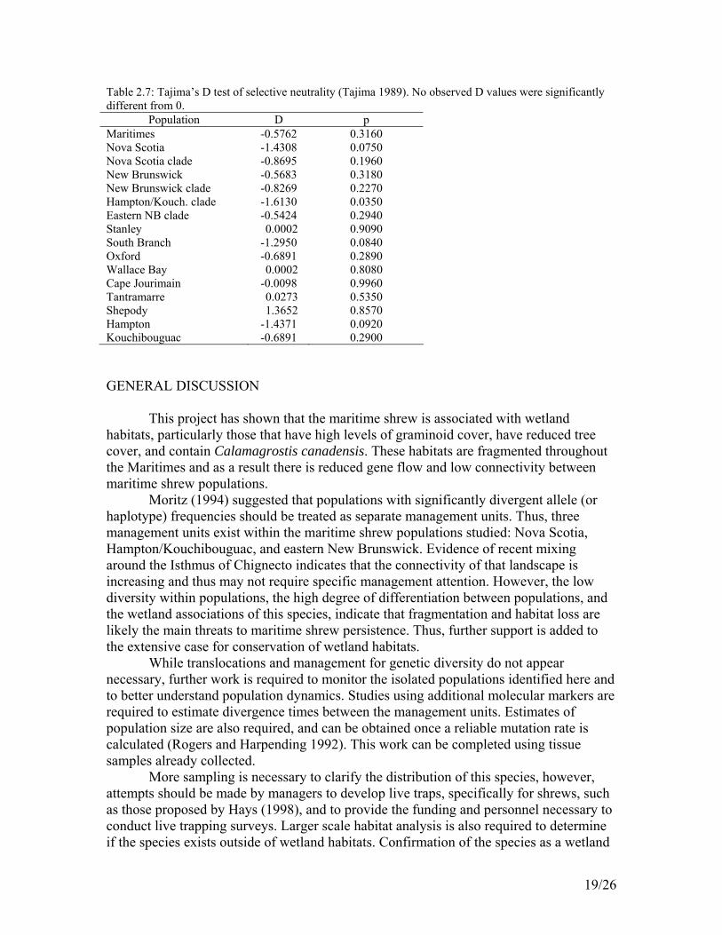
Table 2.7: Tajima’s D test of selective neutrality (Tajima 1989). No observed D values were significantly different from 0.

Population D p Maritimes -0.5762 0.3160 Nova Scotia -1.4308 0.0750 Nova Scotia clade -0.8695 0.1960 New Brunswick -0.5683 0.3180 New Brunswick clade -0.8269 0.2270 Hampton/Kouch. clade -1.6130 0.0350 Eastern NB clade -0.5424 0.2940 Stanley 0.0002 0.9090 South Branch -1.2950 0.0840 Oxford -0.6891 0.2890 Wallace Bay 0.0002 0.8080 Cape Jourimain -0.0098 0.9960 Tantramarre 0.0273 0.5350 Shepody 1.3652 0.8570 Hampton -1.4371 0.0920 Kouchibouguac -0.6891 0.2900 GENERAL DISCUSSION

This project has shown that the maritime shrew is associated with wetland habitats, particularly those that have high levels of graminoid cover, have reduced tree cover, and contain Calamagrostis canadensis. These habitats are fragmented throughout the Maritimes and as a result there is reduced gene flow and low connectivity between maritime shrew populations.

Moritz (1994) suggested that populations with significantly divergent allele (or haplotype) frequencies should be treated as separate management units. Thus, three management units exist within the maritime shrew populations studied: Nova Scotia, Hampton/Kouchibouguac, and eastern New Brunswick. Evidence of recent mixing around the Isthmus of Chignecto indicates that the connectivity of that landscape is increasing and thus may not require specific management attention. However, the low diversity within populations, the high degree of differentiation between populations, and the wetland associations of this species, indicate that fragmentation and habitat loss are likely the main threats to maritime shrew persistence. Thus, further support is added to the extensive case for conservation of wetland habitats.

While translocations and management for genetic diversity do not appear necessary, further work is required to monitor the isolated populations identified here and to better understand population dynamics. Studies using additional molecular markers are required to estimate divergence times between the management units. Estimates of population size are also required, and can be obtained once a reliable mutation rate is calculated (Rogers and Harpending 1992). This work can be completed using tissue samples already collected.

More sampling is necessary to clarify the distribution of this species, however, attempts should be made by managers to develop live traps, specifically for shrews, such as those proposed by Hays (1998), and to provide the funding and personnel necessary to conduct live trapping surveys. Larger scale habitat analysis is also required to determine if the species exists outside of wetland habitats. Confirmation of the species as a wetland

19/26

habitat specialist would further support conservation of these habitats and would facilitate management planning.

Both habitat and genetic analyses support the premise that wetland habitat is required for the persistence of the maritime shrew. Because ecological and genetic issues interact (Lacy 1997), considering both disciplines provides a more complete picture of the issues causing species vulnerability and presents managers with robust information for planning conservation strategies. CONCLUSIONS

The contributions of the Fund allowed this project to be completed as planned. The work is represented in the thesis titled “ Habitat associations and genetic diversity of the maritime shrew (Sorex maritimensis)” and held at Acadia University. It will also be submitted, in smaller units, for publication in peer-reviewed journals. The complete financial report is attached as an appendix to the document. REFERENCES Akaike, H. 1974. A new look at the statistical model identification. IEEE Trans. Auto.

Control AC. 19: 716-723. Astronomical Applications Department. 2003. Fraction of the moon illuminated. US

Naval Observatory. Atlantic Canada Conservation Data Center. 2005. Provincial Lists and Ranks. Tantramar

Interactive Inc. Bellocq, I., J. F. Bendell, and B. L. Cadogan. 1992. Effects of the insecticide Bacillus

thuringiensis on Sorex cinereus (masked shrew) populations, diet, and prey selection in a jack pine plantation in northern Ontario. Canadian Journal of Zoology. 70: 505-510.

Betts, M. G., N. P. P. Simon, and J. J. Nocera. 2005. Point count summary statistics differentially predict reproductive activity in bird-habitat relationship studies. Journal of Ornithology. 146: 151-159.

Blackburn, L. D., and R. D. Andrews. 1992. Higher efficiency of pitfall traps in capturing three shrew species for analysis of diet and habitat. Transactions of the Illinois State Academy of Science. 85: 173-181.

Bohonak, A. J. 1999. Dispersal, gene flow, and population structure. The Quarterly Review of Biology. 74: 21-45.

Branch, L. C., A. M. Clark, and B. W. Bowen. 2003. Fragmented landscapes, habitat specificity, and conservation genetics of three lizards in Florida scrub. Conservation Genetics. 4: 199-212.

Brownlie, J. 1988. A disjunct population of the blue spotted salmander Ambystoma-laterale in southwestern Nova Scotia. Canadian Field Naturalist. 102: 263-264.

Burnham, K. P., and D. R. Anderson 2002. Model Selection and Multimodel Inference. Springer-Verlag, New York.

20/26

Chenna, R., H. Sugawara, T. Koike, R. Lopez, T. J. Gibson, D. G. Higgins, and J. D. Thompson. 2003. Multiple sequence alignment with the Clustal series of programs. Nucleic Acids Research. 31: 3497-3500.

Churchfield, S., V. A. Nesterenko, and E. A. Shvarts. 1999. Food niche overlap and ecological separation amongst six species of coexisting forest shrews (Insectivora: Soricidae) in the Russian Far East. Journal of Zoology, London. 248: 349-359.

Churchfield, S., and B. I. Sheftel. 1994. Food niche overlap and ecological separation in a multi-species community of shrews in the Siberian taiga. Journal of Zoology, London. 234: 105-124.

Churchfield, S., B. I. Sheftel, N. V. Moraleva, and E. A. Shvarts. 1997. Habitat occurrence and prey distribution of a multi-species community of shrews in the Siberian taiga. Journal of Zoology, London. 241: 55-71.

Clement, M., D. Posada, and K. A. Crandall. 2000. TCS: a computer program to estimate gene geneologies. Molecular Ecology. 9: 1657-1660.

Dalthorp, D. 2004. The generalized linear model for spatial data:assessing the effects of environmental covariates on population density in the field. Entomologica Experimentalis et Applicata. 111: 117-131.

Diaz de Pascual, A., and A. A. De Ascencao. 2000. Diet of the cloud forest shrew Cryptotis meridensis (Insectivora: Soricidae) in the Venezuelan Andes. Acta Theriologica. 45: 13-24.

Doak, D. F., and L. S. Mills. 1994. A useful role for theory in conservation. Ecology. 75: 615-626.

Excoffier, L., P. E. Smouse, and J. M. Quattro. 1992. Analysis of molecular variance inferred from metric distances among DNA haplotypes: application to human mitochondrial DNA restriction data. Genetics. 131: 479-491.

Goheen, J. R., R. K. Swihart, T. M. Gehring, and M. S. Miller. 2003. Forces structuring tree squirrel communities in landscape fragmented by agriculture: species differences in perceptions of forest connectivity and carrying capacity. Oikos. 102: 95-103.

Hanley, J. A., and B. J. McNeil. 1982. The meaning and use of the area under a receiver operating characteristic (ROC) curve. Radiology. 143: 29-36.

Hartley, S., and W. E. Kunin. 2003. Scale dependency of rarity, extinction risk, and conservation priority. Conservation Biology. 17: 1559-1570.

Hays, W. S. T. 1998. A new method for live-trapping shrews. Acta Theriologica. 43: 333-335.

Herman, T. B., and F. W. Scott. 1992. Global change at the local level: assessing the vulnerability of vertebrate species to climatic warming. Pages 353 - 367 in W. e. al., editor. Science and the management of protected areas. Elsevier.

Kirkland, G. L., and D. F. Schmidt. 1996. Sorex arcticus. Mammalian Species: 1-5. Kumar, S., K. Tamura, I. B. Jakobsen, and M. Nei. 2001. MEGA2: Molecular

Evolutionary Genetics Analysis software. Arizona State University, Tempe, Arizona, USA.

Lacy, R. 1997. Importance of genetic variation to the viability of mammalian populations. Journal of Mammalogy. 78: 320-335.

Madden, L. V. 2002. Evaluation of generalized linear mixed models for analyzing disease incidence data obtained in designed experiments. Plant Dis. 86: 316-325.

21/26

McCarthy, C. 1996. Chromas 1.45. School of Health Science, Griffith University, Southport, Queensland.

McCay, T. S., and G. L. Storm. 1997. Masked shrew (Sorex cinereus) abundance, diet and prey selection in an irrigated forest. American Midland Naturalist. 138: 268-275.

McLaughlin, J. F., J. L. Hellman, C. L. Boggs, and P. R. Ehrlich. 2002. Climate change hastens population extinctions. Proceedings of the National Academy of Sciences of the United States. 99: 6070-6074.

Mech, S. G., and J. G. Hallett. 2001. Evaluating the effectiveness of corridors: a genetic approach. Conservation Biology. 15: 467-474.

Meteorological Society of Canada. 2002. Climate Data On-line. Environment Canada. Michener, W. K., E. R. Blood, K. L. Bildstein, M. M. Brinson, and L. R. Gardner. 1997.

Climate change, hurricanes and tropical storms, and rising sea level in coastal wetlands. Ecological Applications. 7: 770-801.

Miller, M. P. 1997. Tools for population genetic analyses (TFPGA) 1.3: A Windows progam for the analysis of allozyme and molecular population genetic data. Computer software distributed by author.

Mockford, S. W., L. McEachern, T. B. Herman, M. Snyder, and J. M. Wright. 2005. Population genetic structure of a disjunct population of Blanding's turtle (Emydoidea blandingii) in Nova Scotia, Canada. Biological Conservation. 123: 373-380.

Moritz, C. 1994. Defining 'Evolutionary Significant Units' for conservation. TRENDS in Ecology and Evolution. 9: 373-375.

Mortsch, L. D. 1998. Assessing the impact of climate change on the great lakes shoreline wetlands. Climatic Change. 40: 391-416.

Nagelkerke, N. J. D. 1991. A note on a general definition of the coefficient of determination. Biometrika. 78: 691-692.

Nei, M., and S. Kumar 2000. Molecular Evolution and Phylogenetics. Oxford University Press, New York.

Page, R. D. M., and E. C. Holmes 1998. Molecular Evolution A Phylogenetic Approach. Blackwell Sciences Ltd.

Parmesan, C., and G. Yohe. 2003. A globally coherent fingerprint of climate change impacts across natural systems. Nature. 421: 37-42.

Peltonen, A., and I. Hanski. 1991. Patterns of island occupancy explained by colonization and extinction rates in shrews. Ecology. 72: 1698-1708.

Pfenninger, M., and D. Posada. 2002. Phylogeographic history of the land snail Candidula unifasciata (Hellicellinae, Stylommatophora): Fragmentation, corridor migration, and secondary contact. Evolution. 56: 1776-1788.

Posada, D. version 1.2. available from http://darwin.uvigo.es. Posada, D., and K. A. Crandall. 2001. Intraspecific gene genealogies: trees grafting into

networks. TRENDS in Ecology and Evolution. 16: 37-45. R Development Core Team. 2004. R: A language and environment for statistical

computing. R Foundation for Statistical Computing. Vienna, Austria. Rambaut, A. 1996. Se-Al: Sequence Alignment Editor. Available at

http://evolve.zoo.ox.ac.uk.

22/26

Rogers, A. R., and H. Harpending. 1992. Population growth makes waves in the distribution of pairwise genetic differences. Molecular Biology and Evolution. 9: 552-569.

Rosenberg, M. S. 2001. PASSAGE. Pattern analysis, spatial statistics and geographic exegesis. Department of Biology, Arizona State University, Tempe, AZ.

Rudd, R. L. 1955. Age, sex, and weight comparisons in three species of shrews. Journal of mammalogy. 36: 323 - 339.

Ryan, J. M. 1986. Dietary overlap in sympatric populations of pygmy shrews, Sorex hoyi, and masked shrews, Sorex cinereus, in Michigan. The Canadian Field Naturalist. 100: 225-228.

Schneider, S., D. Roessli, and L. Excoffier. 2000. Arlequin ver. 2.000: A software for population genetics data analysis. Genetics and Biometry Laboratory, Univeristy of Geneva, Switzerland.

Schumaker, N. H. 1996. Using landscape indices to predict habitat connectivity. Ecology. 77: 1210-1225.

Scott, F. W., and A. J. Hebda. 2004. Annotated list of the mammals of Nova Scotia. Proceedings of the Nova Scotian Institute of Science. 42: 189-208.

Stewart, D., and A. J. Baker. 1994. Evolution of mtDNA D-loop sequences and their use in phylogenetic studies of shrews in the subgenus Otisorex (Sorex: Soricidae: Insectivora). Molecular Phylogenetics and Evolution. 3: 38-46.

Stewart, D., N. D. Perry, and L. Fumagalli. 2002. The maritime shrew, Sorex maritimensis (Insectivora: Soricidae): a newly recognized Canadian endemic. Canadian Journal of Zoology.

Swofford, D. L. 2003. PAUP. Phylogenetic Analysis Using Parsimony. Sinauer Associates, Sunderland, Massachusetts.

Tajima, F. 1989. Statistical method for testing the neutal mutation hypothesis by DNA polymorphism. Genetics. 123: 585-595.

Taylor, P. D. 2000. Landscape Connectivity: Linking Fine-Scale Movements and Large-Scale Patterns of Distributions of Damselflies. Pages 109-122 in B. Ekbom, M. Irwin, and Y. Roberts, editors. Interchanges of Insects Between Agricultural and Surrounding Landscapes. Kluwer Academic Publishers, Netherlands.

Volobouev, V. T., and C. G. Van Zyll De Jong. 1988. The karyotype of Sorex arcticus maritimensis (Insectivora, Soricidae) and its systematic implications. Canadian Journal of Zoology. 66.

Wagenmakers, E.-J., and S. Farrell. 2004. AIC model selection using akaike weights. Psyconomic bulletin and review. 11: 192-196.

Wisheu, I. C., C. J. Keddy, P. A. Keddy, and N. M. Hill. 1994. Disjunct Atlantic coastal plain species in Nova Scotia: distribution, habitat and conservation priorities. Biological Conservation. 68: 217-224.

Wright, S. 1965. The interpretation of population structure by F-statistics with special regard to systems of mating. Evolution. 19: 395-420.

Zalba, S. M., and A. J. Nebbia. 1999. Neosparton darwinii (Verbenaceae), a restricted endemic species. Is it also endangered? Biodiversity and conservation. 8: 1585-1593.

23/26

FINANCIAL REPORT BUDGET SUMMARY

New Brunswick Wildlife Trust Fund 58-0-205133 2003/2004 Required items Budgeted Expended Differential Salary 4000.00 5999.15 -1999.15 Travel 1400.00 2089.28 -689.28 Supplies 460.00 930.91 -470.91 Lab supplies 5360.00 1976.00 3384.00 TOTALS 11220.00 10995.34 224.66 Nova Scotia Habitat Conservation Fund 58-0-205132 2003/2004 Required items Budgeted Expended Differential Salary 6400.00 8027.18 -1627.18 Travel 1400.00 460.17 939.83 Supplies/food 480.00 323.78 156.22 Lab supplies 1720.00 788.87 931.13 Management Fee 2000.00 2400.00 -400.00 TOTALS 12000.00 12000.00 0.00 New Brunswick Museum 2003/2004 Required Items Budgeted Expended Differential Salary 1000.00 1000.00 0.00 TOTALS 1000.00 1000.00 0.00 In-Kind Support Required Items Budgeted Expended Differential Assistant's 2400.00 2400.00 0.00 Accomodations 728.00 728.00 0.00 Freezer storage 800.00 800.00 0.00 Camp Equipment 300.00 300.00 0.00 Field supplies 700.00 700.00 0.00 Lab Supplies 1200.00 1200.00 0.00 TOTALS 6128.00 6128.00 0.00 Assistants: 2 pers provided by Don Stewart to aid field and lab work Accomodations: provided by CWS (Sackville), Kouchibouguac National Park, Joe Kennedy (DNR Hampton), and the Read Family (Oxford)

24/26

Freezer Storage: provided by CWS (Sackville) and DNR (Oxford) Camp Equipment: provided by CWS (Sackville) Field Supplies: Obtained from Acadia University (Wolfville, NS) Lab Supplies: Obtained from Acadia University (Wolfville, NS) DETAILED EXPENDITURE REPORT Date Reference Description Expense Balance 12000.0027-Sep 2003 000511 salary 124.70 11875.3011-Oct 2003 000513 salary 124.70 11750.6025-Oct 2003 000515 salary 124.70 11625.908-Nov 2003 000518 salary 124.70 11501.20

22-Nov 2003 000520 salary 124.70 11376.506-Dec 2003 000523 salary 124.70 11251.80

20-Dec 2003 000526 salary 124.70 11127.103-Jan 2004 000528 salary 87.29 11039.81

21-Jun 2004 000493 salary 612.90 10426.915-Jul 2004 000496 salary 408.60 10018.31

19-Jul 2004 000498 salary 408.60 9609.712-Aug 2004 000501 salary 408.60 9201.11

16-Aug 2004 000503 salary 408.60 8792.5130-Aug 2004 000506 salary 408.60 8383.9113-Sep 2004 000508 salary 408.60 7975.3127-Sep 2004 000511 salary 408.60 7566.7111-Oct 2004 000513 salary 163.44 7403.27

To 205133 from 205132 -1430.10 8833.3716-Aug 2004 000503 salary 600.00 8233.3730-Aug 2004 000506 salary 600.00 7633.3712-Jun 2004 J046281 mgmt fee 2400.00 5233.3721-Jun 2004 000493 salary 17.02 5216.3521-Jun 2004 000493 salary 18.02 5198.33

5-Jul 2004 000496 salary 13.56 5184.775-Jul 2004 000496 salary 12.01 5172.76

19-Jul 2004 000498 salary 13.56 5159.2019-Jul 2004 000498 salary 12.01 5147.192-Aug 2004 000501 salary 13.56 5133.632-Aug 2004 000501 salary 12.01 5121.62

16-Aug 2004 000503 salary 36.60 5085.0216-Aug 2004 000503 salary 29.65 5055.3730-Aug 2004 000506 salary 36.60 5018.7730-Aug 2004 000506 salary 29.65 4989.1213-Sep 2004 000508 salary 13.56 4975.5613-Sep 2004 000508 salary 12.01 4963.5527-Sep 2004 000511 salary 13.56 4949.9927-Sep 2004 000511 salary 15.68 4934.3111-Oct 2004 000513 salary 3.90 4930.41

25/26

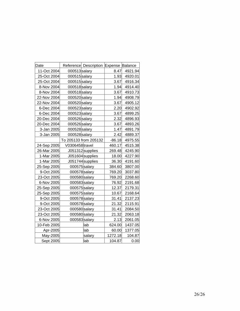
Date Reference Description Expense Balance 11-Oct 2004 000513 salary 8.47 4921.9425-Oct 2004 000515 salary 1.93 4920.0125-Oct 2004 000515 salary 3.67 4916.348-Nov 2004 000518 salary 1.94 4914.408-Nov 2004 000518 salary 3.67 4910.73

22-Nov 2004 000520 salary 1.94 4908.7922-Nov 2004 000520 salary 3.67 4905.126-Dec 2004 000523 salary 2.20 4902.926-Dec 2004 000523 salary 3.67 4899.25

20-Dec 2004 000526 salary 2.32 4896.9320-Dec 2004 000526 salary 3.67 4893.26

3-Jan 2005 000528 salary 1.47 4891.793-Jan 2005 000528 salary 2.42 4889.37

To 205133 from 205132 -86.18 4975.5524-Sep 2005 V0306458 travel 460.17 4515.3826-Mar 2005 J051312 supplies 269.48 4245.901-Mar 2005 J051604 supplies 18.00 4227.901-Mar 2005 J051744 supplies 36.30 4191.60

25-Sep 2005 000575 salary 384.60 3807.009-Oct 2005 000578 salary 769.20 3037.80

23-Oct 2005 000580 salary 769.20 2268.606-Nov 2005 000583 salary 76.92 2191.68

25-Sep 2005 000575 salary 12.37 2179.3125-Sep 2005 000575 salary 10.67 2168.64

9-Oct 2005 000578 salary 31.41 2137.239-Oct 2005 000578 salary 21.32 2115.91

23-Oct 2005 000580 salary 31.41 2084.5023-Oct 2005 000580 salary 21.32 2063.186-Nov 2005 000583 salary 2.13 2061.05

10-Feb 2005 lab 624.00 1437.05Apr-2005 lab 60.00 1377.05

May-2005 salary 1272.18 104.87Sept 2005 lab 104.87 0.00

26/26