FINAL REPORT Electromagnetic Induction E-Sensor for Underwater UXO

Detection

SERDP Project MR-2108

DECEMBER 2011 Dr. Yongming Zhang QUASAR Federal Systems, Inc.

Report Documentation Page Form ApprovedOMB No. 0704-0188

Public reporting burden for the collection of information is estimated to average 1 hour per response, including the time for reviewing instructions, searching existing data sources, gathering andmaintaining the data needed, and completing and reviewing the collection of information. Send comments regarding this burden estimate or any other aspect of this collection of information,including suggestions for reducing this burden, to Washington Headquarters Services, Directorate for Information Operations and Reports, 1215 Jefferson Davis Highway, Suite 1204, ArlingtonVA 22202-4302. Respondents should be aware that notwithstanding any other provision of law, no person shall be subject to a penalty for failing to comply with a collection of information if itdoes not display a currently valid OMB control number.

1. REPORT DATE DEC 2011

2. REPORT TYPE N/A

3. DATES COVERED -

4. TITLE AND SUBTITLE Electromagnetic Induction E-Sensor for Underwater UXO Detection

5a. CONTRACT NUMBER

5b. GRANT NUMBER

5c. PROGRAM ELEMENT NUMBER

6. AUTHOR(S) 5d. PROJECT NUMBER

5e. TASK NUMBER

5f. WORK UNIT NUMBER

7. PERFORMING ORGANIZATION NAME(S) AND ADDRESS(ES) QUASAR Federal Systems, Inc.

8. PERFORMING ORGANIZATIONREPORT NUMBER

9. SPONSORING/MONITORING AGENCY NAME(S) AND ADDRESS(ES) 10. SPONSOR/MONITOR’S ACRONYM(S)

11. SPONSOR/MONITOR’S REPORT NUMBER(S)

12. DISTRIBUTION/AVAILABILITY STATEMENT Approved for public release, distribution unlimited

13. SUPPLEMENTARY NOTES The original document contains color images.

14. ABSTRACT QUASAR Federal Systems (QFS) endeavored to adapt its innovative underwater capacitive electrodeelectric field (E) sensors for use in detection of Unexploded Ordnance (UXO) objects in seawater. Thesystem was based around an existing Time Domain Electromagnetic (TDEM) sensor, in which a pulsedmagnetic (B) field induces eddy currents in the target. The eddy currents produce a secondary B-field,which in a conducting medium can be detected with either E-sensors or B-sensors. The E-sensor was usedto measure decaying eddy currents in a standard UXO-like target. The results were compared to bothpreviously measured B-fields and calculated values for the same target. The E-sensor showed similarresponse to the B-sensor, with roughly 1/3 the signal-to-noise ratio (SNR) but a broader detection range.The E-sensor data from a steel rod were in excellent agreement, in both shape and amplitude, to thecalculated value for a vertical magnetic dipole of moment 0.03 Am2. The UXO detection capability of theQFS underwater E-sensor has been clearly demonstrated. The vector nature of the fields also suggests thesensor could be use for discrimination, using inversion algorithms such as the Time Domain 3-DipoleModel. In future work the detection capability of this sensor will be enhanced and the discriminationpotential will be explored.

15. SUBJECT TERMS

16. SECURITY CLASSIFICATION OF: 17. LIMITATION OF ABSTRACT

SAR

18. NUMBEROF PAGES

33

19a. NAME OFRESPONSIBLE PERSON

a. REPORT unclassified

b. ABSTRACT unclassified

c. THIS PAGE unclassified

Standard Form 298 (Rev. 8-98) Prescribed by ANSI Std Z39-18

Table of Contents

Table of Contents ........................................................................................................................... iii

List of Figures ................................................................................................................................ iv

List of Acronyms ............................................................................................................................ v

Keywords ....................................................................................................................................... vi

Acknowledgements ........................................................................................................................ vi

1.0 Abstract ............................................................................................................................ 1

2.0 Objective .......................................................................................................................... 1

3.0 Background ...................................................................................................................... 2

3.1 Time Domain Electromagnetic Sensing ....................................................................... 2

3.2 QFS underwater E-field electrode ................................................................................ 5

3.3 Calculation of E-field generated by UXO Target ......................................................... 6

4.0 Materials and Methods ..................................................................................................... 9

4.1 Transmitter Optimization ............................................................................................. 9

4.2 Sensor Optimization ................................................................................................... 13

4.3 Sensor Calibration ...................................................................................................... 14

4.4 Integrate Test Bed ....................................................................................................... 17

5.0 Results and Discussion ................................................................................................... 21

5.1 Data Collection ........................................................................................................... 21

5.2 Comparison with B-sensor ......................................................................................... 23

5.3 Comparison with Calculation ..................................................................................... 25

6.0 Conclusions and Future Work ........................................................................................ 26

6.1 Conclusions ................................................................................................................ 26

6.2 Future Work ................................................................................................................ 27

7.0 References ...................................................................................................................... 28

iii

List of Figures Figure 1. Transmit and receive timing for TDEM. Blue: Digital Logic for Tx pulse, Green: Voltage measured at Tx coil, Red: Rx response. Example voltage decay time constants shown. . 4 Figure 2. Illustrating the need to remove the “background” in TDEM measurements. ................. 4 Figure 3. Comparison of QFS (right) and SIO electrodes (left) off the Australian coast (2009). The QFS electrodes were separated by only 80 cm, whereas the SIO electrodes were 12 times further apart (10 m). Data collected at same time and location. ..................................................... 5 Figure 4. Left: QFS underwater E-field sensing electrode assembled/open. Right: 3 channel electrode amplifier .......................................................................................................................... 6 Figure 5. The spherical coordinates for model calculation with the UXO at the center (0,0,0). The sensing plane is at z = h above the center. ...................................................................................... 7 Figure 6. Left: Calculated Eφ from Vertical Magnetic Dipole, over 1x1 m grid at 0.5 m depth. Right: Calculated Bz. Center point is 5, 5. ...................................................................................... 8 Figure 7. Left: Geometry for projection of Eφ onto Ey (top view), Right: Calculated field at Ey sensor. ............................................................................................................................................. 8 Figure 8. Left: H-bridge driver circuit. Right: 190 Am2 Tx coil. Both developed under MM1444.......................................................................................................................................................... 9 Figure 9. Basic schematic of H-bridge driver. Impulse response time is proportional to coil inductance divided by damping resistance. .................................................................................. 11 Figure 10. Improvement of TDEM impulse response .................................................................. 13 Figure 11. Left: Diagram of underwater E-sensor calibration. Right: Modeled conversion between seawater current and E-field inside test fixture. ............................................................. 16 Figure 12. Calibration of single-axis underwater E-sensor. ......................................................... 17 Figure 13. Design choices for 3-axis E-field sensor. Left: Desired configuration. Right: Necessary configuration for 10 cm baseline. ................................................................................ 18 Figure 14. Stray B-field pick up in electrode wiring ................................................................... 19 Figure 15. Photo of 3-axis electrode housing, 14 cm baseline. .................................................... 20 Figure 16. Left: Photo of seawater test bed. Right: Side view diagram of test configuration. ..... 20 Figure 17. Photo of standard UXO-like target used in data collection; 2” diameter, 6” long steel rod. ................................................................................................................................................ 20 Figure 18. E-sensor TDEM response to steel rod; whole decay shown ....................................... 22 Figure 19. Data grid for vertically aligned steel rod; shown for t = 400 µs, shown for Ey (left) and Ez (right) ................................................................................................................................ 22 Figure 20. Top: E-sensor response to steel rod, including scaled measurement to 0.5 m sensor-to-target distance. Bottom: B-sensor response to steel rod for same set-up. ..................................... 24 Figure 21. Grid plots for steel rod target response in By; measured under MM1444 .................. 25 Figure 22. Comparison of measured Ey (left) and calculated Ey (right) for VMD ...................... 26

iv

List of Acronyms µ micro

B-field Magnetic field

DAQ Data Acquisition System

DSA Digital Signal Analyzer

E-field Electric field

EM Electromagnetic

EMF Electromotive force

FET Field Effect Transitor

Hz Hertz

ms millisecond

nV nanoVolt

QFS QUASAR Federal Systems

Rx Receiver

SIO Scripps Institute of Oceanography

SNR Signal-to-noise ratio

SON Statement of Need

TD3D Time Domain Three Dipole

TDEM Time Domain Electromagnetic

TF Transfer Function

TVS Transient Voltage Suppressor

Tx Transmitter

UXO Unexploded Ordnance

VMD Vertical Magnetic Dipole

v

vi

Keywords Unexploded Ordinance, Underwater Electrodes, UXO detection, UXO discrimination, Electromagnetic measurement, Induction sensor, Induction coil, Magnetic measurement, Primary field, Time-Domain Three Dimensional model, Time-domain electromagnetic measurement,

Acknowledgements This material is based upon work supported by SERDP through the Humphreys Engineer Support Activity under Contract No. W912HQ-10-C-0090. Any opinions, findings and conclusions or recommendations expressed in this material are those of the author(s) and do not necessarily reflect the view of the US Army Corps of Engineers, Humphreys Engineer Support Activity.

Electromagnetic Induction E-Sensor for Underwater UXO Detection

1.0 Abstract QUASAR Federal Systems (QFS) endeavored to adapt its innovative underwater capacitive electrode electric field (E) sensors for use in detection of Unexploded Ordnance (UXO) objects in seawater. The system was based around an existing Time Domain Electromagnetic (TDEM) sensor, in which a pulsed magnetic (B) field induces eddy currents in the target. The eddy currents produce a secondary B-field, which in a conducting medium can be detected with either E-sensors or B-sensors. The E-sensor was used to measure decaying eddy currents in a standard UXO-like target. The results were compared to both previously measured B-fields and calculated values for the same target. The E-sensor showed similar response to the B-sensor, with roughly 1/3 the signal-to-noise ratio (SNR) but a broader detection range. The E-sensor data from a steel rod were in excellent agreement, in both shape and amplitude, to the calculated value for a vertical magnetic dipole of moment 0.03 Am2. The UXO detection capability of the QFS underwater E-sensor has been clearly demonstrated. The vector nature of the fields also suggests the sensor could be use for discrimination, using inversion algorithms such as the Time Domain 3-Dipole Model. In future work the detection capability of this sensor will be enhanced and the discrimination potential will be explored.

2.0 Objective The SERDP Statement of Need (SON) calls for the development of sensors to address diverse challenges in the cleanup of munition contaminated areas; including aquatic environments. These sensors need to operate in a variety of environments such as “ponds, lakes, rivers, estuaries, and coastal and open ocean” and must be capable of detecting munitions ranging from 20-mm shells to 2000-lb bombs. This specific program aims to address this need through the development of an underwater TDEM E-field UXO detection sensor. The program employs a B-field transmitter, common to TDEM techniques. The receiver is based around an innovative underwater electrode recently developed by QFS. The underwater electrode is passivated, allowing it to achieve true capacitive coupling to seawater and virtually eliminating electro-chemical effects that plague resistive coupled systems. In this program, QFS sought to prove the UXO detection capabilities of this innovative underwater electrode. The specific goals of the program were:

1

1) Adapt the existing electrode amplifier to operate in the band of 100 Hz to 10 kHz, with a sensitivity of 10 nV/rtHz.

2) Design and build a 3-axis underwater E-sensor with 10-cm baseline in addition to constructing a seawater-based UXO test-bed.

3) Measure TDEM signals from a UXO target with the underwater E-sensor. Compare them to traditional B-field measurements and calculated values.

QFS successfully met all 3 objectives. A 3-axis seawater E-sensor was designed and built, with sensitivity of 5 nV/m/rtHz over the band of interest. TDEM signals were measured from UXO targets. These signals compared favorably to measurements made with a B-field induction sensor, and were in excellent agreement with calculated fields. This program has effectively demonstrated the UXO detection capability of the QFS underwater E-sensor.

3.0 Background Time domain electromagnetic detection is a common method in UXO remediation. It is able to detect targets and can also be used to discriminate them from scrap. Traditionally TDEM employs magnetic sensors to measure induced eddy currents in a target. This method has proved effective for both land and water based applications. Employing E-field sensors for underwater UXO detection is a new concept. The lack of practical-use, low-noise E-field sensors has limited the size of the community familiar with underwater E-field sensing and its related system and noise cancellation issues. In particular capacitively coupled E-field sensing is new and has only been demonstrated to date for frequencies up to 30 Hz.

3.1 Time Domain Electromagnetic Sensing UXO detection has traditionally been done with DC magnetic sensors which measure distortions in the ambient magnetic field. In recent years improved discrimination techniques have been developed which rely on inducing eddy currents in the target. These sensors utilize physics-based models to recover the shape of the measured object, and discriminate threats from scrap. The work in this program relies on one such sensing method called Time-domain electromagnetic measurement. Time-domain electromagnetic measurement is a common method for UXO detection and discrimination. In this type of measurement, a large primary DC magnetic field is applied to the target by a large transmitter (Tx) coil. When the primary field is shut off, it induces eddy currents in nearby metallic objects. The eddy currents generate a secondary field that can be measured by a receiver (Rx) coil. The time decay of the response gives information about the size, shape, orientation, and conductivity of the metal object.

2

TDEM data generally require very little data processing. The responses over numerous pulses are integrated, or stacked, in the receiver. It is convenient to time average or gate in the receiver in real-time, although that can be done in post-processing. Statistical discrimination techniques based on model analysis, such as the Time-Domain Three Dipole (TD3D) model, can separate UXO-like objects from scrap-like ones. In practice TDEM is carried out with an inductive transmitter coil and a DC current source. A DC voltage is applied to the coil for a certain duration (pulse width), during which time a DC field is generated, and then turned off quickly. As soon as the field is shut down, decaying eddy currents are induced in the target and any nearby conductors. An AC magnetic sensor measures the response. Even in the absence of a target, there is still a large decaying voltage, comprising the decaying primary B-field in the Tx coil, the transient response of the receiver, and induced eddy currents in nearby metal; collectively referred to as the “background”. In the case of the QFS TDEM system, the difficulty in measuring the eddy current response from a target is the presence of a large background. The background is often orders of magnitude larger than the secondary field from the target. It is necessary to reliably measure the background, and subtract it from the final data, in order to see the target signal. QFS has built several TDEM systems on previous programs, chiefly SERDP MM1444. An example of TDEM Tx and Rx timing, measured with an early prototype system, is shown in Figure 1. The blue trace shows the digital logic of the transmitter. In the high state the transmitter is ON; DC field is generated. In the low state the transmitter is OFF and the fields begin to decay. The green trace shows the voltage across the transmit coil. During the ON state this voltage is simply the DC voltage of the drive circuit, 12 V. After the drive signal turns off, a back electromagnetic field (EMF) is generated in the coil; ~ 400 V. This back EMF generates a transient in the receiver (red trace), driving it into saturation. Only after the receiver recovers from saturation (~ 250 µs) can useful data be collected. The delay of ~ 40 µs between the logic turning off, and the back EMF, is an RC delay circuit in the transmitter; designed to reduce the magnitude of the back EMF on the driver components. The voltage decay constants, τ, are shown for the transmitter and receiver. These are determined by inductance, resistance, and capacitance in the transmitter and receiver respectively, and must be tuned for fast system recovery.

3

-10

-5

0

5

10

Volta

ge (V

)

4003002001000-100

Time (μs)

-400

-200

0

200

400

Transmitter V

oltage (V)

Drive Signal Transmitter Voltage Receiver Output

Induction Sensor Pulse Timing and Receiver Response

Transmitter Off

τ = 20 μs

τ = 35 μs

Figure 1. Transmit and receive timing for TDEM. Blue: Digital Logic for Tx pulse, Green: Voltage measured at Tx coil, Red: Rx response. Example voltage decay time constants

shown.

An example TDEM B-field measurement is shown in Figure 2 (for a later TDEM system, also on MM1444). The red trace shows the response of a vertical B-field sensor following the transmit pulse; the background is clear and present throughout the entire 10 ms window. The green trace shows the result of subtracting two background measurements. Finally the blue trace shows the response to a standard target (2” diameter, 6” tall steel rod, 0.5 m beneath the receiver) with the background removed.

Figure 2. Illustrating the need to remove the “background” in TDEM measurements.

4

It is evident that at early times (< 1 ms) the target signal is less than or equal to the background signal for the MM1444 system. Without background subtraction, target detection would be very difficult. In practice, accurate removal of the background can be challenging. It depends not only on the decay time of the coil, but also the transmit voltage (which can sag) and the presence of conductive materials in the vicinity of the sensor (which can change). Often the SNR of the system is limited not by the sensitivity of the receiver, but by the accuracy of background subtraction.

3.2 QFS underwater E-field electrode The exploitation of E-fields underwater has been held back by the performance and ease-of-use of technology used to make the electrical interface to the ocean. Prior approaches relied on producing a low electrical resistance contact to the electric potentials of interests via an electrochemical reaction with the sea water. However, this reaction produces offset potentials that depend on temperature, salinity, micro structural differences between the pair of electrodes used, and prior exposure of the electrodes to air and light. These offset potentials can easily be of order millivolts and small changes in the potentials can completely obscure the nanovolt-to-microvolt signals of interest. QFS has developed a revolutionary new type of underwater electrode that is passivated to minimize electrochemical reaction with the seawater. Instead this electrode couples capacitively to the local electric potential. A series of deep ocean tests in locations from Australia to the Gulf of Mexico have demonstrated that this new technology can obtain its theoretical noise floor in real world conditions and after sitting on the deck of a ship for many weeks. The QFS electrodes were compared side-by-side with the prior state-of-the-art underwater Ag/AgCl E-field sensors, developed by the Scripps Institute of Oceanography (SIO). This comparison shows that for comparable baseline the new QFS technology is at least five times more sensitive above 1 Hz, shown in Figure 3. A QFS underwater E-field electrode is shown in Figure 4.

Figure 3. Comparison of QFS (right) and SIO electrodes (left) off the Australian coast

(2009). The QFS electrodes were separated by only 80 cm, whereas the SIO electrodes were 12 times further apart (10 m). Data collected at same time and location.

Hz

E(V/

m/rt

Hz)

or B

(T/rt

Hz)

SIO - BxSIO - BySIO - ExSIO - EySIO - Ez

Bx, By10-12

10-9

Ez

Ex, Ey

Hz

E(V/

m/rt

Hz)

or B

(T/rt

Hz)

SIO - BxSIO - BySIO - ExSIO - EySIO - Ez

SIO - BxSIO - BySIO - ExSIO - EySIO - Ez

Bx, By10-12

10-9

Ez

Ex, Ey

Hz

E(V/

m/rt

Hz)

or B

(T/rt

Hz)

QGeo - BxQGeo - ByQGeo - ExQGeo - EyQGeo - Ez

Bx, By10-12

10-9

Ex, Ey, Ez

Hz

E(V/

m/rt

Hz)

or B

(T/rt

Hz)

QGeo - BxQGeo - ByQGeo - ExQGeo - EyQGeo - Ez

QGeo - BxQGeo - ByQGeo - ExQGeo - EyQGeo - Ez

Bx, By10-12

10-9

Ex, Ey, Ez

5

Figure 4. Left: QFS underwater E-field sensing electrode assembled/open. Right: 3 channel

electrode amplifier

The electrode amplifier for the capacitive electrodes is also shown in Figure 4. The amplifier comprises a front end gain for each electrode, a differential amplifier with switchable gain, and a low pass filter, with a corner frequency of 30 Hz. The through-and-through gain of the board can be set to 250, 500, 1000, or 2000. The sensitivity of the underwater sensor is plotted in Figure 3, ~ 1 nV/m/rtHz above 1 Hz.

3.3 Calculation of E-field generated by UXO Target Electromagnetic signals experience substantial frequency dependent attenuation as they pass through seawater owing to its high conductivity (σ = 4 S/m). While this fact imposes practical limits to the range of E-fields traveling through the water, it also results in very low E-field environmental noise. The following calculation, based on the diagram of Figure 5, shows the possibility of detecting the E-field generated by the magnetic dipole of a UXO target. In the model, the UXO target (source) is represented as a vertical alternating magnetic dipole, with a magnetic moment m, at the seabed. The underwater receiver is located at h above the source.

6

Figure 5. The spherical coordinates for model calculation with the UXO at the center (0,0,0). The sensing plane is at z = h above the center.

The expressions for the EM fields of a vertical magnetic dipole (VMD) are given by Kraichman (1970) for infinite, homogeneous, conducting media, using spherical coordinates with the dipole m along the polar axis (Figure 5). The UXO detection environment is certainly not an infinite, homogenous, conducting medium; however the approximation holds for the extremely near-field nature of UXO detection. The relevant fields for a vertical magnetic dipole are:

rerr

mE γφ γ

θγμω −

⎟⎟⎠

⎞⎜⎜⎝

⎛+−=

11π4sinj , (1)

rr e

rrmH γ

γθγ −

⎟⎟⎠

⎞⎜⎜⎝

⎛+=

11π2cos

2, (2)

rerrr

mH γθ

γγθγ −

⎟⎟⎠

⎞⎜⎜⎝

⎛++=

22

2 111π4

sin , (3)

where γ ( ) is the wave propagation constant in seawater; ω is the angular frequency, r is the radial spherical coordinate, σ is the conductivity of seawater, and ε and µ are the permittivity and permeability of the medium, respectively.

ωμσεμωγ j+−= 22

Using the expressions (1-3), the vertical magnetic field Bz and horizontal electric field Eφ are calculated for a vertical magnetic dipole moved through a grid beneath the sensor. The model assumes m = 0.03 Am2, f = 2.5 kHz, h = 0.5 m, and is calculated over a 1 m x 1 m grid. The amplitude of Eφ and Bz, as a function of the horizontal positions (x,y), is shown in Figure 6.

m

Sensing plane

hr

UXO

Sea floor

X

Y

(0,0)

θ

φ

m

Sensing plane

hr

UXO

Sea floor

X

Y

(0,0)

m

Sensing plane

hrSea floor

X

Y

(0,0)

UXO

θ

φ

7

x y x y

Figure 6. Left: Calculated Eφ from Vertical Magnetic Dipole, over 1x1 m grid at 0.5 m depth. Right: Calculated Bz. Center point is 5, 5.

The Bz field plotted in Figure 6 shows the field directly measured by a vertical B-sensor. By contrast, the Eφ plotted is magnitude of the field; it does not illustrate what is measured by a horizontal E-sensor. To calculate the expected field at the sensor, the calculated Eφ must be projected onto the y-axis. This is achieved by multiplying the value of Eφ by the cosine of the azimuthal angle (in spherical coordinates); taken from the target frame, as in Figure 7. Doing so results in the horizontal E-field (symmetric for Ex and Ey) shown in Figure 7.

x y

Figure 7. Left: Geometry for projection of Eφ onto Ey (top view), Right: Calculated field at Ey sensor.

8

4.0 Materials and Methods Under a previous SERDP contract (MM1444) QFS developed a TDEM sensor system, based around a vector-field magnetic induction sensor. An entire system was constructed, comprising an inductive B-field Tx coil, an H-bridge Tx driver circuit, a 3-axis induction sensor receiver, and a LabVIEW based data acquisition system (DAQ). This system was optimized over the course of several years and used to collect large amounts of TDEM data from UXO-like (metal rods and spheres) and scrap-like (metal disks) objects. The resulting data were processed by Dr. Robert Grimm of Southwest Research Institute, who was able to distinguish UXO-like objects from scrap-like objects in almost all cases [Zhang, 2010]. In short, the TDEM system developed under MM1444 was quite mature, and was essential in the execution of this SEED program. However modifications were necessary to accommodate the particular application of E-field receiving TDEM. The sensors used in this program were based on an underwater E-field sensor system QFS has been developing for geophysics applications. The sensor is a pair of underwater electrodes, and a low noise, high input impedance amplifier. Prior to this program these electrodes and amplifier have been used to collect data in the frequency band of 1 mHz to 30 Hz, with a noise floor of ~ 1 nV/m/rtHz above 1 Hz. Like the TDEM hardware, the sensors were quite mature, but required some modifications for this particular application.

4.1 Transmitter Optimization The B-field transmitter for TDEM was built in a previous SERDP program (MM1444). The transmitter comprises an inductive Tx coil and a DC driver circuit. The Tx coil from that program was 96 turns on a 1 m square coil-form, with the windings stacked to approximate a dipole (rather than a solenoid). The driver circuit was an H-bridge transmitter, run at 24 VDC (with 2 car batteries) and able to drive ~ 2 A through the Tx coil. The resulting magnetic moment of the transmitter was ~ 190 Am2. The driver circuit and Tx coil are shown in Figure 8

Figure 8. Left: H-bridge driver circuit. Right: 190 Am2 Tx coil. Both developed under

MM1444.

9

The first effort at optimizing the transmitter was to improve the stability of the TDEM background. In the previous program the background would drift downward slightly in time, as the voltage of the supply batteries drooped. The car batteries powering the driver circuit were replaced with a high current DC supply, with 8 mF of capacitance in parallel. The DC supply can source up to 10 A, and the capacitors are intended to supply instantaneous current when the supply sags. A quick study was made, running the system ~20 times in quick succession, and looking at reliability of background subtraction. The study indicated an initial sag in the background, as the capacitors and supply arrived at a steady state of current delivery. This suggested both a “warm-up” routine and a well regimented data collection procedure, with experiments spaced evenly in time. The LabVIEW DAQ was modified to accommodate 10 warm-up runs, spaced at 5 s, then continued onto data collected; again spacing runs at 5 s apart. This procedure provided a stable background that could be reliably subtracted. In addition to improving stability of the background, it is also desirable to reduce or eliminate it altogether. In particular, if the recovery time of the transmitter could be shortened to less than 100 µs, it would no longer present an issue to target data collection. To this end the Tx coil and driver circuit were redesigned to achieve lower background and faster recovery, while maintaining roughly the same magnetic moment. The important specifications for the transmitter design are magnetic moment, recovery time, and power consumption. The moment is important because the eddy currents generated in the target are proportional to the field strength and length of transmit pulse. The recovery time is critical because the eddy currents in the target are decaying quickly, and can be masked by decaying field in the Tx coil. Power consumption is a practical matter that will become important if the system is ever deployed to the field. Under the MM1444 program, the design focus was on magnetic moment rather than recovery time. The receiver on that program was a B-field induction sensor, which utilized a high permeability core and low input impedance. The magnetic core and input impedance were both critical to low noise of that sensor, but also resulted in an extremely long impulse response in the receiver; as shown in Figure 2 above. Therefore the transmitter was only designed to recover faster than the receiver, not necessarily as fast as possible. The recovery time of the transmitter is dominated by the decay of the primary field in the inductive Tx coil. That energy is dissipated with a time constant given by ; where L is inductance of the coil, and R is the damping resistor. A basic circuit diagram for the transmitter is shown in Figure 9. The bleed-off resistors are to ensure balanced voltage across the coil in the OFF state.

10

Figure 9. Basic schematic of H-bridge driver. Impulse response time is proportional to coil

inductance divided by damping resistance.

Thus there are two methods to shortening the decay time of the transmitter: either raise R or lower L. In practice there is a limit to how high the damping resistor can be. The back EMF generated in the coil is given by V = RDAMP*ICOIL. The voltage rating of most of the driver components is 1 kV, therefore a hard limit is placed on R. Furthermore, the self resonance of the inductive Tx coil must be considered. If the resonant frequency is within the band of interest, the damping resistor must be tuned to achieve critical damping in the coil. The original MM1444 coil has an inductance of 23 mH and a self resonance at ~ 30 kHz. The damping resistor on that transmitter was tuned to achieve critical damping of the Tx coil (~ 2 kΩ) and the voltage protection on the driver was provided by transient voltage suppressors (TVS) across the coil, rated at 400 V. Transient voltage suppressors serve to shunt any voltage in excess of their rating. This provides over-voltage protection to the driver, but also shorts out the damping resistor. Anytime spent in the TVS clamped mode is lost time. Thus there is a trade-off between protecting the driver and fast recovery of the circuit. Under MM1444 the damping resistor, TVS’s, and slow turn-off of the FETs were all tuned to ensure the transmitter decay time was faster than that of the B-field induction sensors. The resulting time constant of this original transmitter was τ ~ 100 µs. Under the current program, the receiver does not use magnetic materials of any kind and has high input impedance. In theory ultra-fast recovery is possible in the receiver. Thus considerable effort was put into speeding up the recovery of the transmitter. The goal was to completely shunt the transmit field to below noise levels, before decay measurements began (approximately 100 µs after the transmit pulse ends).

11

A new Tx coil was built with 1/3 the turns of the MM1444 coil. Inductance is proportional to number of turns, N, squared. Thus in reducing the coil from 96 turns to 30 turns, the new inductance was ~ 9x lower. The series resistance of the coil was also reduced by 1/3, so though the number of turns went down, the drive current went up; leaving magnetic moment roughly the same. The transient voltage suppressors in the drive circuit were beefed up to 900 V. This gave much higher head room for the damping resistor, while still maintaining a safety margin for the 1 kV limit. The damping resistor was chosen such that the back EMF did not exceed the 900 V rating, eliminating the lost clamp time of the previous circuit. The slow turn off delay in the driver, illustrated in Figure 1 above, was eliminated, saving an additional 40 µs. Lastly, an E-field shield was installed on the Tx coil. Several layer of Aluminum foil were wrapped around the coil, with a gap in the middle to prevent formation of a B-field pick-up loop. The shield was connected to the system ground of the receiver and Tx driver circuit. Furthermore a capacitive plate was placed in the water tank, and also connected to the system ground. It was found that tying all grounds, including the bath, resulted in lower sensor noise. Through all these efforts, the decay time constant of the transmitter was reduced from τ ~100 µs to τ ~20 µs. A measurement of the transmitter voltage showed a recovery from 900 V to 100 µV (~140 dB) in 250 µs (data not shown). However, ultimately it is not the transmitter voltage which is important, as much as the measured background in the receiver. There is a direct correlation between the two, but the measured background has many other contributions. Improvement of the TDEM background was measured with the underwater E-field receiver, Figure 10. The red trace shows the background for the original (MM1444) transmit coil and H-bridge driver circuit. The blue trace was recorded with the same sensor, after improvements were made to coil and driver. While the decay constant of the transmitter alone is τ ~ 20 µs (data not shown), the overall system decay time constant is τ ~ 1.2 ms (blue trace, Figure 10). The blue trace shows a clear improvement over the red; however there is still a significant background signal. This is largely attributed to the impulse response of the sensor; it is unclear whether the slow response is in the amplifier circuit or the electrodes themselves. In future work it will be desirable to redesign the electrodes and amplifier with fast recovery in mind.

12

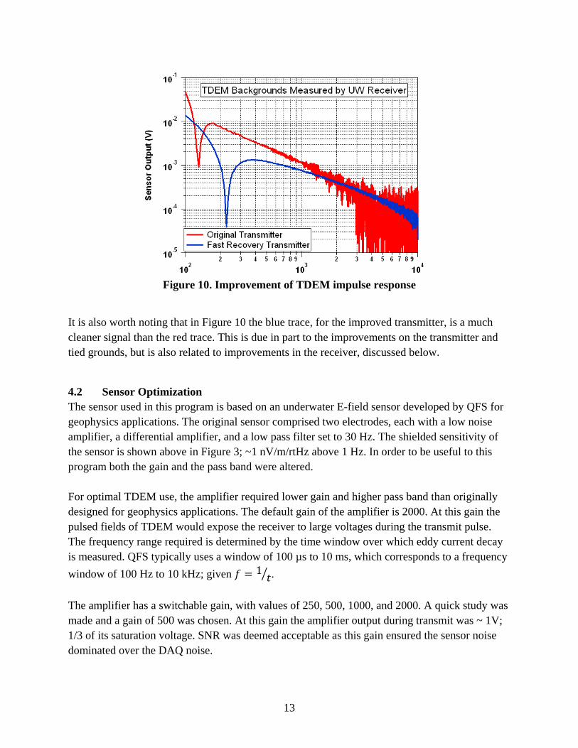
Figure 10. Improvement of TDEM impulse response

It is also worth noting that in Figure 10 the blue trace, for the improved transmitter, is a much cleaner signal than the red trace. This is due in part to the improvements on the transmitter and tied grounds, but is also related to improvements in the receiver, discussed below.

4.2 Sensor Optimization The sensor used in this program is based on an underwater E-field sensor developed by QFS for geophysics applications. The original sensor comprised two electrodes, each with a low noise amplifier, a differential amplifier, and a low pass filter set to 30 Hz. The shielded sensitivity of the sensor is shown above in Figure 3; ~1 nV/m/rtHz above 1 Hz. In order to be useful to this program both the gain and the pass band were altered. For optimal TDEM use, the amplifier required lower gain and higher pass band than originally designed for geophysics applications. The default gain of the amplifier is 2000. At this gain the pulsed fields of TDEM would expose the receiver to large voltages during the transmit pulse. The frequency range required is determined by the time window over which eddy current decay is measured. QFS typically uses a window of 100 µs to 10 ms, which corresponds to a frequency window of 100 Hz to 10 kHz; given 1 . The amplifier has a switchable gain, with values of 250, 500, 1000, and 2000. A quick study was made and a gain of 500 was chosen. At this gain the amplifier output during transmit was ~ 1V; 1/3 of its saturation voltage. SNR was deemed acceptable as this gain ensured the sensor noise dominated over the DAQ noise.

13

The built-in low pass filter on the amplifier was bypassed altogether, setting the pass band to upwards of 50 kHz. However it soon became clear that the system was experiencing elevated noise due to aliasing. It was simultaneously found that the output impedance of the amplifier was too high for the DAQ. The National Instruments’ DAQ used in this program, also originally developed for MM1444, requires a source impedance < 1 kΩ, due to a switching capacitor multiplexor. Source impedances in excess of 1 kΩ lead to “ghosting” (charge injection from one channel to the next) and elevated noise. The output of the amplifier was altered to a single pole, low pass filter with a corner frequency of 2.5 kHz. (In future systems it will be desirable to use a higher order, higher frequency low pass filter, to ensure fidelity of the early time data.) The output impedance was simultaneously set at 500 Ω. Lastly protection circuitry was installed on the input of the amplifier. A cross-diode pair of Schottky diodes, with turn-on voltage of 0.12 V, was installed across the terminals of the two electrodes. The intent of this circuit was to short circuit the electrodes when they experience a voltage difference in excess of 0.12 V; hopefully avoiding saturation of the amplifier. In practice this circuit was ineffective, given the high gain of the amplifier. Since the saturation voltage is ±3 V, the turn on of the Schottky’s would need to be 500x smaller than that, or 6 mV. In spite of their ineffectiveness, the Schottky diodes were left in place, as a protection against any mistakes during experimentation.

4.3 Sensor Calibration Sensor calibration followed the modification/optimization stage. Calibration involves measuring the sensitivity and effective baseline of the sensor. Sensitivity is the measured noise floor of the sensor, expressed in units of field (V/m). Since the sensor is two electrodes and an amplifier, conversion of noise (V) to sensitivity (V/m) requires dividing the measured noise by the baseline of the sensor. In principle the baseline can be measured simply with a ruler. If the electrodes are perfect voltage probes, then the baseline is simply the geometric distance between them. In practice there are field distortions resulting from materials in the vicinity of the electrodes, whether conducting or insulating. Therefore the effective baseline must be measured electronically. QFS is accustomed to measuring effective baseline of E-sensors in air. QFS owns a calibration capacitor; a pair of 3 m disks separated by 1 m, which generate a uniform field in their center. An air-based E-sensor is placed inside, a known field is applied, and the sensor response is measured.

14

Typical measurement of the effective baseline takes the form a transfer function (TF). A voltage is applied to the capacitor and fed back into Ch1 of a Digital Signal Analyzer (DSA). The sensor response is fed into Ch2 of the DSA. The DSA then records Ch2/Ch1 as a function of frequency. This TF measurement is Vout/Vapp. However the applied voltage is across the plates of the capacitor, therefore it is an applied field. Therefore the TF is actually Vout/Eapp = Vout/(Vapp/d) = Vout/Vapp*d. Since d = 1 m, the TF is a measure of baseline (including sensor gain), and is in units of meters. To find the actual effective baseline the TF is finally divided by the gain of the sensor. QFS typically builds 2-paddle, air-based E-sensors, with a geometric baseline of 10 cm. The measured effective baseline of these sensors comes out closer to 7 cm. In water the above calibration procedure will not work. Charge will flow in a conductor to screen any applied E-fields. Supposing underwater electrodes were placed inside the QFS calibration capacitor in a seawater bath, it is safe to assume the seawater would shield the sensor from most, if not all, of the applied E-field. One might then ask what an underwater E-sensor actually measures in seawater. It makes much more sense to discuss currents, in a conductor, than E-fields. Thus the sensors are probing a voltage as it is dropped in the resistive medium. Under the current program a new calibration procedure for underwater E-sensors was devised and executed, based on this principle. Where normally a field is applied through the air (capacitively), now the field would be applied as a current through the water (resistively). A new calibration fixture was built: a capacitor with 32 cm diameter plates, separated at 64 cm, with a 10 Ω series resistor. The capacitor was placed in a volume of water, large compared to size of the cal fixture, and a single-axis E-sensor was located in the middle, Figure 11. The fixture was driven by the DSA as before, but instead of feeding the drive voltage back to Ch1, the voltage across the series resistor was measured. In this way the TF measured was Vout/Iapp. The difficulty then lies in converting the applied current to an equivalent E-field.

15

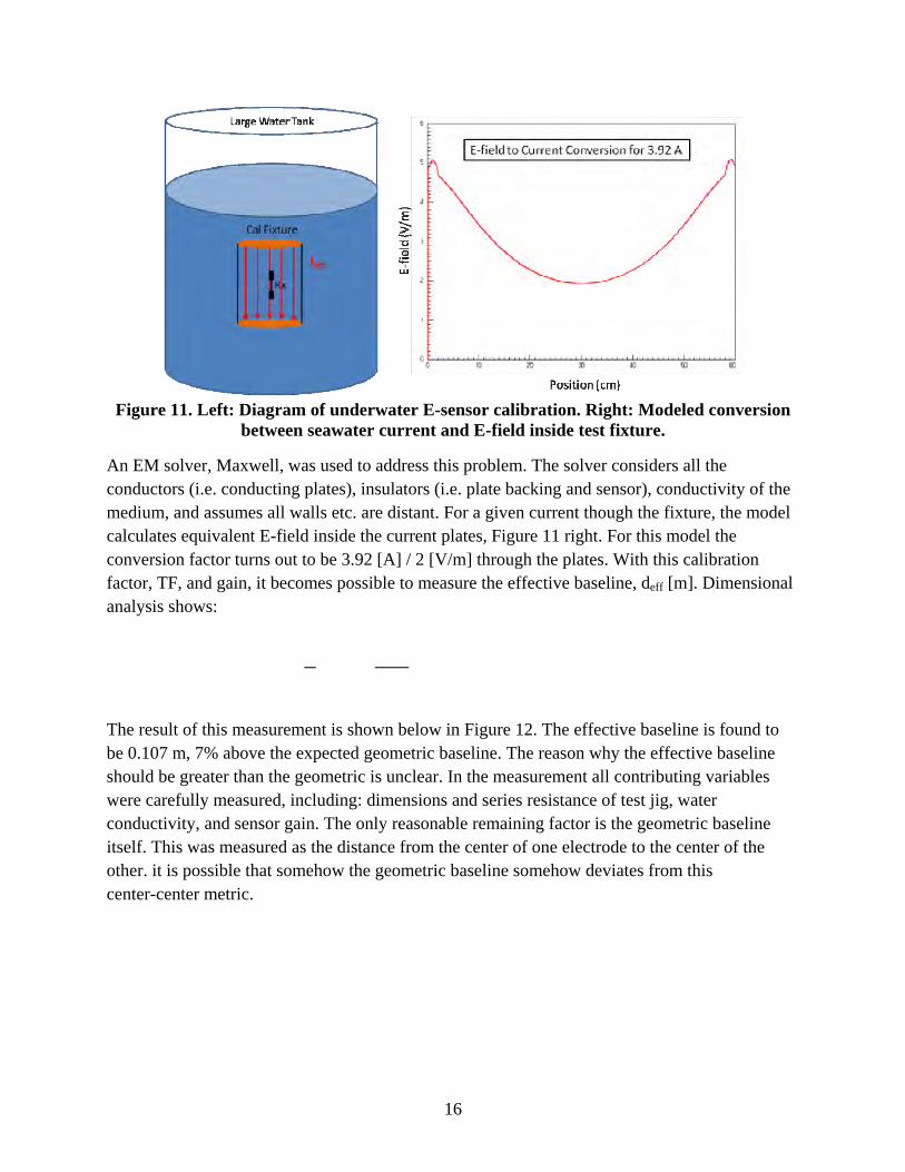
Figure 11. Left: Diagram of underwater E-sensor calibration. Right: Modeled conversion

between seawater current and E-field inside test fixture.

An EM solver, Maxwell, was used to address this problem. The solver considers all the conductors (i.e. conducting plates), insulators (i.e. plate backing and sensor), conductivity of the medium, and assumes all walls etc. are distant. For a given current though the fixture, the model calculates equivalent E-field inside the current plates, Figure 11 right. For this model the conversion factor turns out to be 3.92 [A] / 2 [V/m] through the plates. With this calibration factor, TF, and gain, it becomes possible to measure the effective baseline, deff [m]. Dimensional analysis shows:

The result of this measurement is shown below in Figure 12. The effective baseline is found to be 0.107 m, 7% above the expected geometric baseline. The reason why the effective baseline should be greater than the geometric is unclear. In the measurement all contributing variables were carefully measured, including: dimensions and series resistance of test jig, water conductivity, and sensor gain. The only reasonable remaining factor is the geometric baseline itself. This was measured as the distance from the center of one electrode to the center of the other. it is possible that somehow the geometric baseline somehow deviates from this center-center metric.

16

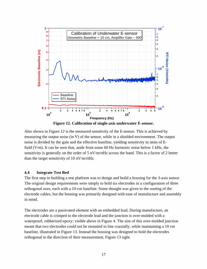
Figure 12. Calibration of single-axis underwater E-sensor.

Also shown in Figure 12 is the measured sensitivity of the E-sensor. This is achieved by measuring the output noise (in V) of the sensor, while in a shielded environment. The output noise is divided by the gain and the effective baseline, yielding sensitivity in units of E-field (V/m). It can be seen that, aside from some 60 Hz harmonic noise below 1 kHz, the sensitivity is generally on the order of 5 nV/m/rtHz across the band. This is a factor of 2 better than the target sensitivity of 10 nV/m/rtHz.

4.4 Integrate Test Bed The first step in building a test platform was to design and build a housing for the 3-axis sensor. The original design requirements were simply to hold six electrodes in a configuration of three orthogonal axes, each with a 10-cm baseline. Some thought was given to the routing of the electrode cables, but the housing was primarily designed with ease of manufacture and assembly in mind. The electrodes are a passivated element with an embedded lead. During manufacture, an electrode cable is crimped to the electrode lead and the junction is over-molded with a waterproof, rubberized epoxy; visible above in Figure 4. The size of this over-molded junction meant that two electrodes could not be mounted in line coaxially, while maintaining a 10 cm baseline, illustrated in Figure 13. Instead the housing was designed to hold the electrodes orthogonal to the direction of their measurement, Figure 13 right.

0.1

2

3

4

5

6

7

8

91

Elec

tron

ic B

asel

ine

(m)

102

2 3 4 5 6 7 8

103

2 3 4 5 6 7 8

104

2 3 4 5

Frequency (Hz)

10-9

2

3

4567

10-8

2

3

4567

10-7

RTI N

oise (V/m/rtH

z)

Calibration of Underwater E-sensorGeometric Baseline = 10 cm, Amplifier Gain ~ 500

Baseline RTI Noise

17

Figure 13. Design choices for 3-axis E-field sensor. Left: Desired configuration. Right:

Necessary configuration for 10 cm baseline.

The two electrode arrangements shown in Figure 13 will both measure fields along the same axis. Since the E-field is simply the difference in the voltages divided by the distance, the orientation of the electrode is not critical. However the original configuration (right) did result in an unfortunately large loop of electrode wires. As preliminary measurements with this sensor began, the signals did not agree well with calculated values. Furthermore the pattern of the fields seemed a better match for B-fields than E-fields. To probe this effect further, measurements were made where the electrodes, shown in Figure 13 right, were compared to a loop of wire, of comparable area, connected to the same amplifier. Three rough areas were tested, applying a Tx field aligned for maximum B-field pick-up, Figure 14. In all three cases electrodes and wire loop had similar response, indicating stray B-field pick-up in the electrode wiring. For the case of minimal area (green traces) no B-field pick up is evident.

18

Figure 14. Stray B-field pick up in electrode wiring

10-6

10-5

10-4

10-3

10-2

10-1

100

Sens

or O

utpu

t (V)

1002 3 4 5 6 7 8 9

10002 3 4 5 6 7 8 9

10000Time (us)

Big Area Loop Small Area Loop Closed-Down Loop Large Electrodes Small Area Electrodes Minimal Area Electrodes

Electrodes vs Wire Loop with Comparable AreaMeasured for Direct Pulsed Field

The B-field pick up evident in Figure 14 can be attributed to the design of the amplifier. The electrode amplifier has high input impedance. The electrode wires form a loop with non-zero area, and the conductive seawater closes the loop. Although the seawater has much lower conductivity than the copper in the electrode wires, the bulk of the voltage drop is across the high impedance of the amplifier input. In effect, this configuration approximates the B-field induction sensor used in the previous SERDP program (MM1444), with a single turn. Fortunately, the green trace of Figure 14 indicates that by minimizing the area of the loop, stray B-field pick up is eliminated. Thus the E-field sensor housing was redesigned to accommodate minimal wiring loops at the electrodes, similar to Figure 13 left. This required a slight lengthening of the baseline, to 14 cm; Figure 15. The sensor was not recalibrated at this baseline, instead it was assumed to be roughly 14 cm, as supported by the original calibration. This resulted in an overall increase in sensitivity, since it is given by Vnoise/dbaseline. A large water tub was chosen as the test bed. The tub is 5 feet long, 3 feet wide, and 3 feet deep, and was filled with 350 gallons of salt water, to about 2.5 feet deep. The Tx coil was positioned such that the coil windings sit just at the surface of the water. The Rx is suspended 25 cm beneath the Tx coil, both to provide standoff from large voltages on the Tx coil and to ensure it was well within the conducting medium. A 1 m x 1 m sheet of plastic was parceled out into a 10 x 10 grid, of 10 cm squares. The test grid was located 50 cm beneath the Tx coil (25 cm beneath the Rx), Figure 16.

19

Figure 15. Photo of 3-axis electrode housing, 14 cm baseline.

Figure 16. Left: Photo of seawater test bed. Right: Side view diagram of test configuration.

The target used was a standard UXO-like test object. It is a 2” diameter, 6” inch long steel rod. This target was chosen because it is of intermediate size, but its regular geometry yields good SNR for detection experiments. The absence of points or rounded edges ensures the eddy current signals from target accurately approximate a magnetic dipole.

Figure 17. Photo of standard UXO-like target used in data collection; 2” diameter, 6” long

steel rod.

20

5.0 Results and Discussion The UXO-like target was run through the test grid, vertically and horizontally aligned. The data collected was compared to comparable data, collected with a magnetic induction sensor for the same target and depth. The data was also compared to theoretical calculation of the expected fields. The vertically aligned target produced data that compare favorably with both B-sensors and calculated E. The horizontally aligned target did not produce as high a quality of data; this is believed to be an issue with boundary conditions of the test set-up.

5.1 Data Collection An experiment consists of collecting TDEM data from a target from every point on the test grid. The test grid comprises 100 10-cm squares. During an experiment the target is placed in the center of each square in succession. Data are collected at each location. The test grid is located 0.5 m beneath the Tx coil and 0.25 m beneath the receiver. The typical distance measurement, used previously for B-field sensors in MM1444, is from the bottom of the Tx coil to the bottom of the target. During that previous program, B-sensor data were collected for a distance of 47 cm. Consistent with this, E-sensor data were collected at 50 cm. Note: the distance of 50 cm was chosen over 47 cm out of convenience; the difference of 3 cm is deemed negligible. A single data collection consists of 100 stacked averages. A bipolar pulse is applied with the transmitter, and the decay signals are measured after each. The bipolar pulse is stacked and averaged, to eliminate DC offset and background noise. All together, 50 pairs of pulses are averaged for a single run (100 pulses). The data are displayed as a single decay trace for the given collection. An example of this type of data is shown above in Figure 2. During analysis a time gate is chosen from the data. Data are collected from 100 µs out to 10 ms. A typical time gate to choose is 400 µs; at this early time SNR is quite good and the frequency corresponds to a well behaved portion of the pass band. The time gate can be converted to an equivalent frequency according to: f = 1/(t). Thus 400 µs corresponds to ~ 2.5 kHz. The data presented are shown at 400 µs, and the corresponding calculations are run at 2.5 kHz. Two experiments were run with the steel rod target; vertical alignment (+z) and horizontal alignment (+y). The results can be plotted either as the full decay at one grid location, Figure 18, or as one time window at all grid locations, Figure 19.

21

Figure 18. E-sensor TDEM response to steel rod; whole decay shown

y x x y

Figure 19. Data grid for vertically aligned steel rod; shown for t = 400 µs, shown for Ey (left) and Ez (right)

The decay signal from the target can be seen clearly in Figure 18. The centered target has excellent SNR (~200) decaying to the end of window. This plot clearly demonstrates the detection capability of the E sensor. The horizontal E-field shown in Figure 19 shows a well behaved pattern. The Ex data (not shown) are roughly the same amplitude (within a factor of 2) but rotated 90°, as expected. The model for a VMD does not suggest the presence of any E-field in the z-axis. However the Ez plot clearly shows the field in that axis. The measured signal is much too large to be stray B-field

22

pick up, yet theoretically no Ez should be present. The effect could be attributed to the boundary conditions of the water tank, or possibly the fact that the z-axis is not centered in over the grid. Data were also collected for a horizontally aligned target. The data were generally of a lesser quality (not shown). This is believed to be an effect of boundary conditions. The model assumes an infinite, conducting medium. For the case of a vertically aligned target in a large bath, this approximation appears to hold. However when the target is horizontally aligned, this approximation no longer holds. In particular, the azimuthal E-field of Eqn 1 must circulate through an air-water-ground interface at the bottom of the tank. In future work it will be interesting to measure horizontally aligned targets in conditions with well behaved boundary conditions; say the littoral zone of the ocean.

5.2 Comparison with B-sensor The experimental configuration described above endeavored to duplicate that used for B-sensor measurements in MM1444. However certain logistical issues made exact duplication of the previous set-up difficult. In this experiment the transmitter-to-target distance, and thus the induced dipole in the target, is the same between these E-sensor measurements and the previous B-sensor measurements. However in the previous B-field measurements the sensor-to-Tx coil distance was 0; whereas in this experiment it is 0.25 cm. Though the induced signal in the target is the same for both E and B experiments, the former will have stronger signal by virtue of having the receiver closer to the target. A direct comparison between the current E-sensor measurements and the previous B-sensor measurements is possible, simply by scaling the amplitude of the E-field. Equation 1 above allows for calculation of E as a function of position and depth. Plugging in identical positions and magnetic moment, but depths of 0.25 and 0.5 m, yields a difference of a factor of 3. Therefore the signal plotted above in Figure 18 can be scaled to a comparable distance as B. A side-by-side comparison of E-field and B-field TDEM responses is given in Figure 20. The top figure shows the E-sensor response as before, with the amplitude scaled down by a factor of 3 (dotted line). It is evident that both E-field and B-field responses show similar characteristics. Both decay with roughly the same time constant. The scaled E-signal has a maximum SNR of ~ 70, while the B-signal has a max SNR of ~ 200. Both show more than adequate SNR for detection, though the overall SNR of the B-sensor appears superior. A grid plot from the B-sensor measurement (from the MM-1444 project) is shown in Figure 21. The grid patterns look very similar to that of Figure 19 left, but rotated 90°. Even the amplitudes

23

make rough sense. In the near field the relationship between E and B can be found with Faraday’s law:

or | | | |

For a B-field amplitude of 40 pT and frequency of 2.5 kHz, an E-field of roughly 9.6 µV/m is expected. Indeed the B amplitude is 40 pT and if the E amplitude is scaled down by 3, it is ~ 13 µV/m.

10-6

10-5

10-4

10-3

10-2

10-1

Sen

sor O

utpu

t (V

)

2 3 4 5 6 7 8 91000

2 3 4 5 6 7 8 910000

Time (μs)

Target Centered Below Receiver (5, 5) Target on Edge of Grid (0, 0)

B-sensor Response to Steel Rod at 47 cm DepthShown for Target Centered and on Edge of Grid

Figure 20. Top: E-sensor response to steel rod, including scaled measurement to 0.5 m

sensor-to-target distance. Bottom: B-sensor response to steel rod for same set-up.

24

y x

Figure 21. Grid plots for steel rod target response in By; measured under MM1444

5.3 Comparison with Calculation Equations 1-3 allow for direct calculation of the expected E-fields from a vertical magnetic dipole. A side-by-side comparison of measured and calculated Ey is shown in Figure 22. Excellent agreement is found between calculated and experimental values; both show the same basic shape across the grid. If the target is assumed to have magnetic moment m = 0.03 Am2 (which is reasonable), the amplitude between measured and calculated is identical. It is concluded from this comparison that the sensor is accurately measuring E-fields from the UXO target.

25

y y x x

Figure 22. Comparison of measured Ey (left) and calculated Ey (right) for VMD

6.0 Conclusions and Future Work In conclusion this program saw the development of a 3-axis underwater E-field sensor that is capable of detecting UXO targets, at least to 0.5 m. The sensor was calibrated and the sensitivity was shown to be 5 nV/m/rtHz over the band of interest (100 Hz to 10 kHz). The sensor was optimized for TDEM measurements. This novel underwater sensor was combined with an existing TDEM data collection system, which underwent modifications to facilitate UXO detection with E-sensors. The sensor and TDEM system were combined and E-sensor data were collected for a standard UXO-like target. The TDEM E-sensor data collected with E-sensors performed well, agreeing almost exactly with the calculated value, and also compared well with similar B-sensor measurements.

6.1 Conclusions Though the E-sensor appears to have lower SNR than the B-sensor, this program has revealed several potential advantages of using E-sensors. From the model it is evident that while the B-field is center peaked, the E-field has a donut shape with a minimum in the center. The maximum E-field is about 14 µV/m at a radius of 0.25 m from the center and varies by about a factor of 2 over the grid. By contrast the B-sensor has a centered peaked response that falls off ~50x as the target is moved out to the edge of the grid. The E-field signal is not quite as strong as the B-field, but area of maximum signal is much larger for the E than for B. This will make detection easier, since larger portion of the Tx “halo” gives good SNR with an E-field receiver. High SNR over a broader range of the Tx “halo” will

26

result in higher fidelity data inversion for TD3D modeling. Furthermore, E-sensors could simplify logistics of field deployment. The increased area of sensitivity will reduce over-pass requirements of a scanning sensor and make the detection faster with less integration time. It is lastly possible that the center-peaked B-response and the donut-shaped E-response are highly complementary. In future systems it may be desirable to combine E-sensors and B-sensors for a complete mapping of the target. In summary, this program has shown:

1. UXO detection using TDEM is possible with the novel QFS underwater E-sensor. 2. An SNR of at least 70 is possible with this sensor, at a stand-off of 0.5 m. 3. Future work is warranted to optimize the detection capability of this sensor system and to

begin to explore its discrimination capabilities.

6.2 Future Work Calculation and experiment show that a magnetic dipole emits vector E-fields and B-fields. This vector field behavior can be exploited to not only detect, but actually discriminate threat objects. It has previously been shown that a 3-axis vector B-field sensor allows discrimination of target shape, using algorithms such as the Time Domain 3 Dipole (TD3D) model [Zhang, 2010]. The work in this program highlights E-sensors as a potential candidate for continuation of this development. QFS believes this new underwater E-sensor is a novel approach to UXO detection in seawater, with the potential to add data quality, SNR, and new capabilities. We plan to propose a follow-on program to continue optimization of the detection capability of this sensor, as well as develop its target discrimination capabilities. Specifically, QFS would propose:

1. Redesign of E-field amplifier for ultrafast recovery, with a view to “no-background” E-field TDEM.

2. Perform the measurement in a larger water tank to simulate the real world case of targets sitting at the interface of sea water and sediments.

3. Explore the combination of E-sensors and B-sensors for underwater UXO detection/discrimination, and noise cancellation.

4. Build an integrated E/B receiver, possible a 6-axis sensor (3 E, 3 B). 5. Characterize the combined E/B receiver with measurements of UXO-like and scrap-like

objects. 6. Refine and test a TD3D algorithm for UXO detection/discrimination in the seawater

environment.

27

28

7.0 References 1. Kraichman, M. B. 1970. Chapter 3.1, Handbook of Electromagnetic Propagation in Conducting

Media. NAVMAT P-2302. 2. Y.M. Zhang, M. Steiger, A.D. Hibbs, and R. Grimm, T. Sprott, “Dual-mode, Fluxgate-Induction

Sensor for UXO Detection and Discrimination”, JEEG, June 2010, Vol. 15, pp51-64, 2010