final report fdot project number: bdk75-977-73 … … · a database of properties of concrete mix...
TRANSCRIPT
i
Final Report
FDOT Project Number: BDK75-977-73
Development of Design Parameters for Virtual Cement and
Concrete Testing
Principal Investigator: Christopher Ferraro
Graduate Student Assistant: Benjamin Watts
December 2013
Department of Civil Engineering
Engineering School of Sustainable Infrastructure and Environment
College of Engineering
University of Florida
Gainesville, Florida 32611

ii
Disclaimer
The opinions, findings, and conclusions expressed
in this publication are those of the authors and not
necessarily those of the State of Florida Department
of Transportation or the U.S. Department of
Transportation.
Prepared in cooperation with the State of Florida
Department of Transportation and the U.S.
Department of Transportation.

iii
Approximate Conversions to SI Units (from FHWA)
Symbol When You Know Multiply By To Find Symbol
Length
in inches 25.4 millimeters mm
ft feet 0.305 meters m
yd yards 0.914 meters m
mi miles 1.61 kilometers km
Area
in2 square inches 645.2 square millimeters mm2
ft2 square feet 0.093 square meters m2
yd2 square yard 0.836 square meters m2
mi2 square miles 2.59 square kilometers km2
Volume
fl oz fluid ounces 29.57 milliliters mL
gal gallons 3.785 liters L
ft3 cubic feet 0.028 cubic meters m3
yd3 cubic yards 0.765 cubic meters m3
NOTE: volumes greater than 1000 L shall be shown in m3
Mass
oz ounces 28.35 grams g
lb pounds 0.454 kilograms kg
Temperature (exact degrees)
°F Fahrenheit 5 (F-32)/9
or (F-32)/1.8
Celsius °C
Illumination
fc foot-candles 10.76 lux lx
fl foot-Lamberts 3.426 candela/m2 cd/m2
Force and Pressure or Stress
lbf pound-force 4.45 newtons N
lbf/in2 pound-force per square inch 6.89 kilopascals kPa

iv
.
1. Report No. 2. Government Accession No. 3. Recipient's Catalog No.
4. Title and Subtitle
Development of Design Parameters for Virtual Cement and Concrete
Testing
5. Report Date
December, 2013
6. Performing Organization Code
7. Author(s)
Christopher C. Ferraro & Benjamin E. Watts
8. Performing Organization Report No.
00102739/00102730
9. Performing Organization Name and Address
Department of Civil and Coastal Engineering
Engineering School of Sustainable Infrastructure & Environment
University of Florida
365 Weil Hall – P.O. Box 116580
Gainesville, FL 32611-6580
10. Work Unit No.
11. Contract or Grant No.
BDK75-977-73
12. Sponsoring Agency Name and Address
Florida Department of Transportation 605 Suwannee Street, MS 30
Tallahassee, FL 32399
13. Type of Report and Period Covered
Final Report 07/01/12 – 12/31/13
14. Sponsoring Agency Code
15. Supplementary Notes
Prepared in cooperation with the U.S. Department of Transportation and the Federal Highway Administration
16. Abstract
The development, testing, and certification of new concrete mix designs is an expensive and time-consuming aspect
of the concrete industry. A software package, named the Virtual Concrete and Cement Testing Laboratory (VCCTL),
has been developed by the National Institute of Standards and Technology as a tool to predict the performance of
concrete mixes quickly using computer simulation of the hydration behavior of concrete. This software requires
thorough characterization of the raw materials of a concrete mix design in order to accurately model the hydration
reactions. A two-phase testing program was implemented to evaluate the how well the VCCTL software can predict
concrete performance. The techniques required to characterize portland cement were developed and implemented to
provide input data for the VCCTL software. The resulting virtual materials were simulated, and a second testing
program was performed on physical specimens to evaluate the accuracy of those simulations. The accuracy with
which the software simulated basic properties of concrete, such as strength, elastic modulus, and time of set, were
examined.
The process of acquiring cement phase volume and surface area fraction data has been improved substantially
through the use of automated scanning electron microscopy. This has resulted in a more efficient process to obtain
cement characterization data for use in the VCCTL software. Comparison of isothermal calorimetry data and
corresponding time of set data has shown that a typical Type F high-range water-reducing admixture
(superplasticizer) delayed time of set and shifted the main silicate hydration peak by the same amount of time. At the
dosages explored within this study, the delay was proportional to the dosage rate.
The empirical predictions for compressive strength, which were based on elastic modulus and developed for
concretes using coarse aggregates that were mineralogically and/or microstructurally different than typical Florida
limestone aggregates, were not accurate for concretes made with Florida limestone. More work is needed to
accurately predict compressive strength based on the elastic properties of concrete containing Florida limestone
coarse aggregates. A more fundamental approach to the simulation of concrete strength should be investigated.
Detailed characterization of the elastic properties of Florida limestones used to produce coarse aggregates for
portland cement concrete should be performed. A database of properties of concrete mix designs containing Florida
aggregate for use with the VCCTL software and other projects should be created.
The VCCTL software was found to be an effective tool for the simulation of elastic modulus of portland cement

v
concrete, provided the materials being simulated are properly characterized. The VCCTL software currently does not
have a means to incorporate the effects of admixtures on cement hydration. An initial attempt to integrate the effects
of a water-reducing admixture, using heat of hydration data, was successful for a Type F water reducer, but the
software significantly underestimated the setting time for a Type D water reducer. More work is needed to reliably
incorporate the effects of admixtures into the VCCTL software.
There are a number of materials that can be modeled in the VCCTL software that were not considered for this
research. There is support for both fly ash and blast furnace slag hydration in the VCCTL software, though the
accuracy of the model in this respect is largely unknown. The techniques required to characterize these materials are
also more involved due to the significant glassy (amorphous) phase contents of their compositions. The methods by
which these materials can be characterized and the accuracy with which they are simulated in the VCCTL software
should be explored.
17. Keywords.
Cement paste; VCCTL; virtual testing; concrete
modeling; concrete strength; concrete modulus of
elasticity
18. Distribution Statement
No restrictions.
19. Security Classif. (of this report)
Unclassified
20. Security Classif. (of this page)
Unclassified
21. Pages
134
22. Price

vi
ACKNOWLEDGMENTS
The Florida Department of Transportation (FDOT) is acknowledged for their tremendous
contribution to this study. The FDOT State Materials Office provided a significant amount of
testing equipment, materials, and personnel used to complete this research. Sincere gratitude is
extended to the Project Manager Dr. H. D. DeFord. Special acknowledgement is given to Mr.
Michael Bergin for his guidance and assistance throughout this project. The authors would like
to thank Dr. H.R. Hamilton and Dr. Kurtis Gurley for their scholarly input throughout the
project. Sincere acknowledgment is to Mr. Richard DeLorenzo for his contributions to this work,
which include laboratory planning and assistance. Additionally, we thank Mr. Patrick Carlton,
Mr. Thomas Frank, Mr. Jose Armenteros, and Mr. Patrick Gallagher for their assistance with this
research. Their assistance and advice was invaluable. Much of this research would have been
impossible without the help and cooperation of Dr. Amelia Dempere and the other staff at the
University of Florida Major Analytical Instrumentation Center. Thanks also to Dr. Jeffrey
Bullard, Dr. Edward Garboczi, Dr. Paul Stutzman, and Dr. Dale Bentz, from the National
Institute for Standards and Testing, for their assistance.

vii
EXECUTIVE SUMMARY
Background
The development of a tool to predict the properties of portland cement concrete has been
the focus of many avenues of research and development. The complexity of the reactions that
occur during cement hydration precluded the development of useful computational models of the
process until the late 1980s. Over the last 12 years, software known as the Virtual Cement and
Concrete Testing Laboratory (VCCTL) has been available for commercial use from the National
Institute of Standards and Technology (NIST). This software incorporates microstructural
modeling of portland cement hydration, and allows for the prediction of different properties of
the hydrated product. The efficacy of the model relies on the proper characterization of the
materials being simulated. While the potential usefulness of this tool is substantial, its accuracy,
particularly with regards to materials endemic to the state of Florida, has yet to be systematically
evaluated.
Research Requirements
Evaluating the accuracy of the VCCTL software requires the comparison of the predicted
property values for virtual concrete specimens with the actual property values determined for
cured concrete specimens. Elastic modulus and compressive strength for the cured product, and
time of set for the plastic product, are the primary predictive outputs for the mix design being
modeled. Accurate measurement of these properties for a given concrete is necessary for a valid
comparison with the predicted values. Accuracy of the predicted values depends heavily on the
accuracy of the input values for the raw materials, which requires that the raw materials are
properly characterized. The methods and procedures required for this characterization must be
developed and refined.
Research Objectives
The primary objective of this research was to determine the degree of accuracy with
which the VCCTL software can predict the various properties of portland cement concrete
produced with raw materials typically used in the state of Florida. The specific tasks to meet this
objective were as follows:

viii
1. Determine the accuracy with which the VCCTL software predicts the elastic modulus,
compressive strength, and setting time of portland cement concrete.
2. Determine if the software can accurately account for the effects of a water-reducing
admixture (WRA) on setting time by using isothermal calorimetry data obtained from
cementitious samples containing the WRA.
3. Perform sensitivity analyses to evaluate the influence of each material property input on
the degree of accuracy with which the above properties are predicted by the software.
A secondary objective of this research was to examine methods of expediting the acquisition of
raw material characterization data used for inputs to VCCTL software.
Main Findings
The main findings from this study are summarized as follows:
1. The VCCTL software was found to be an effective tool for the prediction of elastic
modulus of portland cement concrete, provided the raw materials used in the simulation
were properly characterized.
2. At the current stage of development, the VCCTL software did not accurately predict the
compressive strength of portland cement concrete using Florida limestone coarse
aggregate. This is expected to be resolved by improving the accuracy of the raw material
property inputs, and by making modifications to the software programming.
3. The VCCTL software currently does not have a means to incorporate the effects of
admixtures on cement hydration. An initial attempt to integrate the effects of a water-
reducing admixture, using heat of hydration data, was successful for a Type F water
reducer, but the software significantly underestimated the setting time for a Type D water
reducer. More work is needed to reliably incorporate the effects of admixtures into the
VCCTL software.
4. The process of acquiring cement phase volume and surface area fraction data has been
improved substantially through the use of automated scanning electron microscopy. This
has resulted in a more efficient process to obtain cement characterization data for use in
the VCCTL software.
5. The empirical predictions for compressive strength, which were based on elastic modulus
and developed for concretes using coarse aggregates that were mineralogically and/or
microstructurally different from typical Florida limestone, were not accurate for

ix
concretes made with Florida limestone. More work is needed to accurately predict
compressive strength based on the elastic properties of concrete containing Florida
limestone coarse aggregates.
6. Comparison of isothermal calorimetry data and corresponding time of set data has shown
that a typical Type F high-range water-reducing admixture (superplasticizer) delayed
time of set and shifted the main silicate hydration peak by the same amount of time. At
the dosages explored within this study, the delay was proportional to the dosage rate.
7. Higher dosage rates of Type F high-range water-reducing admixture (superplasticizer)
typically resulted in an increase in both elastic modulus and compressive strength, when
compared to the control mixes.
Recommendations
Based on the findings from this study, the following recommendations were made:
1. The conclusions drawn from the work performed in this research point to many potential
avenues for future research, both to improve the accuracy of the model as well as to
explore different material inputs and outputs.
2. The empirical compressive strength model built into the VCCTL software, which is
based on elastic modulus, does not accurately predict compressive strength for concrete
mixtures which incorporate Florida limestone. Generalized empirical predictions for
strength of concrete are inherently limited due to the variability of the materials used in
its production. A more fundamental approach to the simulation of concrete strength
should be investigated.
3. Detailed characterization of the elastic properties of Florida limestones used to produce
coarse aggregates for portland cement concrete should be performed. A database of
properties of concrete mix designs containing Florida aggregate for use with the VCCTL
software and other projects should be created.
4. The VCCTL software supports the modeling of admixtures if the specific phase surface
deactivation behavior of the admixture is known. Methods of obtaining this information,
either through material testing, or possibly from the admixture manufacturer, should be
investigated.
5. There are a number of materials that can be modeled in the VCCTL software that were
not considered for this research. There is support for both fly ash and blast furnace slag

x
hydration in the VCCTL software, though the accuracy of the model in this respect is
largely unknown. The techniques required to characterize these materials are also more
involved due to the significant glassy (amorphous) phase contents of their compositions.
The methods by which these materials can be characterized and the accuracy with which
they are simulated in the VCCTL software should be explored.

xi
TABLE OF CONTENTS
page
ACKNOWLEDGMENTS ............................................................................................................. vi
EXECUTIVE SUMMARY .......................................................................................................... vii
TABLE OF CONTENTS ............................................................................................................... xi
LIST OF TABLES ....................................................................................................................... xiv
LIST OF FIGURES .......................................................................................................................xv
INTRODUCTION ...........................................................................................................................1
Background ...............................................................................................................................1
Model Function .........................................................................................................................1
Research Requirements ............................................................................................................2
Hypothesis ................................................................................................................................2
Research Objectives ..................................................................................................................2
Research Approach ...................................................................................................................3
LITERATURE REVIEW ................................................................................................................5
Portland Cement Hydration ......................................................................................................5
Cement Heat of Hydration ........................................................................................................7
Admixtures ...............................................................................................................................9
Strength of Concrete ...............................................................................................................10
Scanning Electron Microscopy ...............................................................................................11
Computer Modeling ................................................................................................................13
Cementitious Simulation ........................................................................................................15
Background ......................................................................................................................15
History .............................................................................................................................16
Validation of CEMHYD3D ....................................................................................................20
Existing Research using the VCCTL Software ......................................................................22
Current Limitations of the VCCTL Software .........................................................................24
Other Cementitious Modeling Software .................................................................................25
VCCTL SOFTWARE MATERIAL INPUTS ...............................................................................27
Overview .................................................................................................................................27
xii
Model Inputs for Portland Cement .........................................................................................28
Microstructural Inputs .....................................................................................................29
Gypsum Phase Mass Fractions ........................................................................................29
Cement Phase Volume and Surface Area Fractions, Two Point Correlation
Functions ......................................................................................................................29
Cement Particle Size Distribution ...................................................................................31
Cement Particle Shape Data ............................................................................................32
Cement Particle Dispersion .............................................................................................32
Binder System Size ..........................................................................................................33
Hydration Modeling Inputs.....................................................................................................33
Isothermal Conduction Calorimetry – ASTM C 1702 ....................................................33
Curing Conditions ...........................................................................................................39
Aggregate Input Data ..............................................................................................................39
SEM MICROANALYSIS .............................................................................................................40
Overview .................................................................................................................................40
Sample Preparation .................................................................................................................40
Procedures Developed by NIST ......................................................................................40
Improvements to Sample Preparation .............................................................................41
Backscatter Electron and X-Ray Map Image Acquisition ......................................................46
Image Processing ....................................................................................................................50
Creation of Segmented Image .........................................................................................53
Automated Cement Characterization ......................................................................................57
VCCTL SOFTWARE OUTPUT DATA .......................................................................................63
Overview .................................................................................................................................63
Continuous Measurements......................................................................................................64
Periodic Measurements ...........................................................................................................67
Elastic Modulus ...............................................................................................................67
Hydrated Cement Microstructure Modulus .....................................................................68
Concrete and Mortar Modulus .........................................................................................69
Compressive Strength ......................................................................................................70
PHYSICAL TEST PROGRAM .....................................................................................................73
xiii
Physical Testing Program .......................................................................................................73
Isothermal Calorimetry ...........................................................................................................76
COMPARISON OF PHYSICAL TEST DATA TO MODEL OUTPUTS ...................................78
Experimental Design ..............................................................................................................78
Simulation Procedures ............................................................................................................79
Results.....................................................................................................................................80
Water to Cement Ratio Study ..........................................................................................80
Input Sensitivity Study ....................................................................................................87
Admixture Time of Set ....................................................................................................91
Discussion of Results ............................................................................................................100
Modulus of Elasticity and Compressive Strength .........................................................100
Model Sensitivity ...........................................................................................................106
Admixture Influence on Set Time .................................................................................106
CONCLUSIONS AND RECOMMENDATIONS ......................................................................107
Conclusions...........................................................................................................................107
Recommendations .................................................................................................................108
LIST OF REFERENCES .............................................................................................................109
MATHEMATICAL EQUATIONS REFERENCE FOR THE CALCULATION OF
ELASTIC MODULI USING DIFFERENTIAL EFFECTIVE MEDIUM THEORY .........114
SEM FIELD RAW DATA...........................................................................................................116

xiv
LIST OF TABLES
Table page
Table 4-1: Grinding and Polishing Procedure ...............................................................................45
Table 4-2: Volume and Surface Area Fraction Averages ..............................................................56
Table 4-3: Standard Deviations of Volume and Surface Area Fraction Measurements ................56
Table 4-4: Average Difference Between two Image Sets ..............................................................58
Table 4-5: XRD Cement Phase Fraction vs. SEM Microanalysis Measurements .........................61
Table 6-1: Mixture Design Summary ............................................................................................73
Table 6-2: Summary of Test Results for Fresh Concrete ..............................................................74
Table 6-3: Tests and Ages..............................................................................................................77
Table B-1: Fields Acquired At RJ Lee ........................................................................................116
Table B-2: Fields Acquired At UF...............................................................................................116

xv
LIST OF FIGURES
Figure page
Figure 2-1: Heat evolution of Portland Cement ...............................................................................8
Figure 2-2: Heat of Hydration Curve for Portland Cement .............................................................8
Figure 2-3: Scanning Electron Microscope (Goldstein, et al., 2007) ............................................11
Figure 2-4: Beam interaction volume, showing different signal emission regions (Wittke,
2008) ..................................................................................................................................12
Figure 2-5: Particle Size Distribution ............................................................................................15
Figure 2-6: Computer Generated Concrete Structure using “morphological law” (Wittmann,
Roelfstra, & Sadouki, 1984-1985) .....................................................................................17
Figure 2-7: Initial microstructures of (a) real cement, (b) model with spherical particles and
(c) model with real particle shapes ....................................................................................21
Figure 3-1: Cement input Screen of the VCCTL ...........................................................................28
Figure 3-2: Cement Phase Data Input Screen ................................................................................30
Figure 3-3: Cement Particle Size Distribution ...............................................................................31
Figure 3-4: Microstructure Simulation Parameters........................................................................32
Figure 3-5: Simple Isothermal Calorimeter ...................................................................................34
Figure 3-6: Admix Ampoule ..........................................................................................................35
Figure 3-7: Tam Air Isothermal Calorimeter with sample and admix ampoule loaded ................36
Figure 3-8: Hydration Simulation Input Parameters ......................................................................37
Figure 4-1: Saphir 550 Semi Automated Grinder Polisher ............................................................42
Figure 4-2: Optical Microscope .....................................................................................................44
Figure 4-3: Evaporative Carbon Coater .........................................................................................46
Figure 4-4: Cement Grain Close-up ...............................................................................................47
Figure 4-5: BSE Image as Used for Phase Analysis ......................................................................48
Figure 4-6: Elemental Map for Sulfur ...........................................................................................49
Figure 4-7: Maps required to distinguish Alite, Belite, Aluminate, Ferrite, and Gypsum ............49
Figure 4-8: Phase Classification ....................................................................................................51
Figure 4-9: Image Classification Dialog ........................................................................................52
Figure 4-10: Statistical Analysis of Classification.........................................................................52
xvi
Figure 4-11: Segmented Image ......................................................................................................53
Figure 4-12: Segmented Image Prior to Thresholded Blur Operation ...........................................54
Figure 4-13: Segmented Image after Blur .....................................................................................55
Figure 4-14: Fields Analyzed by UF and RJ Lee Group ...............................................................57
Figure 4-15: New false color image ...............................................................................................59
Figure 4-16: After processing, ready for classification .................................................................60
Figure 4-17: Final Cement Image ..................................................................................................61
Figure 5-1: Continuous Measurements Display Page ....................................................................64
Figure 5-2: Fraction Solids Connected Curve ...............................................................................66
Figure 5-3: Periodic Measurement Display Page ..........................................................................67
Figure 5-4: Predicted Young’s modulus vs. time, w/c 0.4 .............................................................71
Figure 5-5: Predicted Strength vs. time, w/c 0.4............................................................................71
Figure 5-6: Strength vs. Elastic Modulus, w/c 0.4 .........................................................................72
Figure 6-1: Preparation of Cylinders .............................................................................................75
Figure 6-2: Compressive Strength and Elastic Modulus Testing ..................................................75
Figure 6-3: Time of Set Test Apparatus ........................................................................................76
Figure 7-1: Compressive Strength vs. Time for different w/c ratios .............................................80
Figure 7-2: Young’s Modulus vs. Time for different w/c ratios....................................................81
Figure 7-3: Power vs. Time for different w/c ratios ......................................................................82
Figure 7-4: Energy vs. Time for different w/c ratios .....................................................................82
Figure 7-5: Young Modulus vs. Time, w/c ratio of 0.4 .................................................................83
Figure 7-6: Compressive Strength vs. Time. w/c ratio of 0.4 ........................................................83
Figure 7-7: Young Modulus vs. Time, w/c ratio of 0.45 ...............................................................84
Figure 7-8: Compressive Strength vs. Time. w/c ratio of 0.45 ......................................................84
Figure 7-9: Young’s Modulus vs. Time. w/c ratio of 0.5 ..............................................................85
Figure 7-10: Compressive Strength vs. Time. w/c ratio of 0.5 ......................................................85
Figure 7-11: Young’s Modulus vs. Time, w/c ratio of 0.55 ..........................................................86
Figure 7-12: Compressive Strength vs. Time, w/c ratio of 0.55 ....................................................86
Figure 7-13: Young’s Modulus vs. Time, Removal of Calorimetry Data .....................................87
Figure 7-14: Young’s Modulus vs. Time, Removal of Cement Particle Shape Data ....................88
Figure 7-15: Young’s Modulus vs. Time, Removal of Aggregate Shape Data .............................88

xvii
Figure 7-16: Young’s Modulus vs. Time, Larger Virtual Microstructure .....................................89
Figure 7-17: Young’s Modulus vs. Time, Different Aggregate Moduli........................................90
Figure 7-18: Fraction Solids Connected vs. Elapsed time .............................................................91
Figure 7-19: Measured Strength vs. Time for Different Admixtures ............................................93
Figure 7-20: Measured Young’s Modulus vs. Time for Different Admixtures .............................93
Figure 7-21: Young’s Modulus vs. Time, 2 oz/cwt TYPE D ........................................................94
Figure 7-22: Young’s Modulus vs. Time, 2 oz/cwt TYPE F .........................................................95
Figure 7-23: Young’s Modulus vs. Time, 4 oz/cwt TYPE F .........................................................95
Figure 7-24: Strength vs. Time, 4 oz/cwt TYPE D........................................................................96
Figure 7-25: Strength vs. Time, 2 oz/cwt TYPE F ........................................................................96
Figure 7-26: Strength vs. Time, 4 oz/cwt TYPE F ........................................................................97
Figure 7-27: Power vs. Time .........................................................................................................98
Figure 7-28: Energy vs. Time ........................................................................................................98
Figure 7-29: Fraction Solids Connected vs. Time .........................................................................99
Figure 7-30: Penetration Resistance vs. Time, Different Admixtures and Dosages ...................100
Figure 7-31: Simulated vs. Measured Elastic Modulus ...............................................................101
Figure 7-32: Strength vs. Elastic Modulus with VCCTL Power Fit and ACI 318 ......................102
Figure 7-33: Crushed Cylinder Fragments ..................................................................................105

1
CHAPTER 1. INTRODUCTION
Background
The development of a tool to predict the properties of portland cement concrete has been
the focus of many avenues of research and development. The complexity of the reactions that
occur during cement hydration precluded the development of useful computational models of the
process until the late 1980s due to the limitations of available computational resources. Over the
last 12 years, software known as the Virtual Cement and Concrete Testing Laboratory (VCCTL)
has been available for commercial use from NIST (The National Institute of Standards and
Technology). This software incorporates microstructural modeling of portland cement hydration,
and allows for the prediction of different properties of the hydrated product. The efficacy of the
model relies on the proper characterization of the materials being simulated. While the potential
usefulness of this tool is substantial, its accuracy, particularly with regards to materials endemic
to the state of Florida and the simulation of the properties of concrete specifically, has yet to be
systematically evaluated.
Model Function
The VCCTL software uses data from real raw materials to create a virtual concrete from
which different material properties can be obtained via virtual testing. The model first creates a
three-dimensional representation of a portland cement suspension, as would exist at the initial
moment of mixing the cement and water. The phase composition of this representation is drawn
directly from the data supplied for the cement being modeled. In a process that mimics the actual
hydration of portland cement, the model then virtually hydrates this three-dimensional
microstructure using a specific set of rules drawn from the observed hydration kinetics and
thermodynamics of portland cement. As the virtual microstructure is hydrated, parameters such
as heat released, total porosity, degree of hydration, and many others are calculated in real time.
When hydration is complete, a finite element calculation, performed on the mesh derived from
the virtual microstructure, provides the elastic modulus of the paste. This elastic modulus can
then be used in combination with the elastic properties of the coarse and fine aggregate to predict
the modulus of the concrete itself. Finally, compressive strength is predicted from this modulus
using a simple empirical relationship.

2
Research Requirements
Evaluating the accuracy of the VCCTL software requires the comparison of the predicted
properties of a given concrete with the actual properties of physical specimens. Elastic modulus,
compressive strength, and time of set are the easily measured predictive outputs of the model,
and knowledge of the actual values of these properties for a given concrete mixture design is
essential to ensure accuracy. It is critical that proper characterization of the materials being
simulated is performed. This requires implementation and refinement of the existing
characterization methods and procedures.
Hypothesis
The Virtual Cement and Concrete Testing Laboratory software predicts the properties of
concrete by modeling the hydration of portland cement based on a simulated microstructure. The
accuracy with which this simulation takes place is highly dependent upon the accuracy with
which the materials being simulated are characterized. The processes by which these materials
are characterized may also be made faster and more accurate through the development of new
techniques and the utilization of modern instrumentation.
Research Objectives
The primary objective of this research was to determine the degree of accuracy with
which the VCCTL software is capable of predicting the various properties of Portland cement
concrete. The specific objectives were as follows:
Determine the accuracy with which the VCCTL software predicts the elastic
modulus, compressive strength, and setting time of portland cement concrete.
Determine the VCCTL software’s ability to account for the effects of water-reducing
admixtures on time of set through the use of heat of hydration data from isothermal
calorimetry.
Evaluate the influence of different material data on the degree of accuracy with which
the above properties are predicted.
A secondary objective of this research was to examine the possibility of expediting the processes
required to characterize the different materials being simulated.

3
Research Approach
The VCCTL software requires detailed information on the input parameters for the
material being simulated within the model to provide accurate simulations. The information,
termed “inputs” for the purpose of this research, are obtained via the thorough characterization of
the materials using laboratory testing methods. Some of this material data is obtained through
standard test methods, however the development of specific and complex characterization
techniques is necessary for the acquisition of certain material properties. The development and
improvement of techniques for the characterization of materials was an initial goal and a
significant portion of the work performed for this research. The testing program for the
development of material inputs utilized the following material analysis techniques:
Scanning electron microscopy and energy dispersive x-ray spectroscopy
microanalysis ;
Isothermal conduction calorimetry;
Laser particle size distribution analysis;
X-ray powder diffraction (XRD) analysis.
These characterization techniques provided the following inputs for use with the VCCTL
software:
Volume and surface area fractions for the different primary portland cement phases;
Heat of hydration of portland cement;
Particle size distribution of portland cement; and
Mass fractions of sulfate phases in portland cement.
The other major initiative of this research was the investigation of the ability of the
VCCTL software to make accurate predictions for different properties of concrete. A study to
evaluate the predictions of elastic modulus, compressive strength, and time of set for concrete
was constructed to determine the accuracy of the VCCTL software. Secondary aspects of this
study included a sensitivity analysis of the software for material inputs, as well as an
experimental technique to calibrate the model to include the effects of different admixtures. A
physical testing program was implemented to provide information on concrete mixtures against
which to compare the results of the model. The following physical tests were performed on fresh
and hardened concrete:

4
Air Content (ASTM C173);
Slump (ASTM C143);
Unit Weight (ASTM C138);
Temperature (ASTM C1064);
Time of Set (ASTM C403);
Compressive Strength (ASTM C39);
Compressive Elastic Modulus (ASTM C469).
Of these tests, time of set, elastic modulus and compressive strength were compared to
predictions made by the VCCTL. Other tests, such as slump, unit weight, temperature, and air
content were performed as part of standard mixing procedure for quality control purposes.
5
CHAPTER 2. LITERATURE REVIEW
Manufacture of Portland Cement
The raw materials required to manufacture portland cement must supply calcium oxide
(CaO or C in common cement chemistry notation), silica (SiO2 or S), alumina (Al2O3 or A), and
hematite (Fe2O3 or F), which are needed to form the four primary phases; Tricalcium silicate
(alite, C3S), dicalcium silicate (belite, C2S), tricalcium aluminate (aluminate, C3A), and
tetracalcium aluminoferrite (ferrite, C4AF). The oxides needed to form the four primary phases
are typically supplied by some combination of limestone, chalk, slate, and clay, proportioned to
give the desired composition on an oxide basis (Mindess & Young, 1981).
Portland cement clinker is manufactured in a rotary kiln, where temperatures at the raw
material inlet, at the top of the kiln, are about 450°C, and steadily increase to about 1450° to
1500°C at the clinker discharge at the bottom of the kiln. The mineralogical composition of the
cement clinker is determined primarily by the maximum processing temperature, time spent by
the raw materials at the maximum temperature, and the rate of cooling. The aluminate and ferrite
phases begin to form by solid state diffusion reactions at approximately 1200°C, and the phases
then melt at approximately 1350°C. The liquid phase formed acts as a flux, which accelerates the
reactions and partially fuses the material into clinker form as it reaches temperatures of at least
1450°C. It is in this latter stage of production where most of the calcium silicates are formed.
Portland cement is obtained when the portland cement clinker is interground with gypsum
(calcium sulfate dihydrate, CaSO4∙2H2O, CS̅H2, where sulfate = SO3 = S̅), which is added to
prevent the concrete experiencing a flash set from the hydration of C3A (Neville, 2011).
Portland Cement Hydration
When mixed with water, portland cement undergoes a complex set of reactions that result
in the transformation of a slurry of cement particles in water to an interconnected solid matrix of
hydration products. The rate and resulting products of this reaction are governed largely by the
relative concentrations of the four major constituents of portland cement: alite (C3S), belite
(C2S), aluminate (C3A), and ferrite (C4AF). A fifth mineral component, gypsum (CS̅H2), plays an
important role in the early stages of the hydration reaction (Mindess & Young, 1981).
The aluminate and ferrite phases react relatively quickly, but their hydration products add
little to the composite strength of the cement. Aluminate is the most readily soluble of the
6
compounds present in portland cement such that if its proportion is too large, the result will be an
immediate stiffening of the cement paste, known as “flash set.” The presence of gypsum within
the portland cement is to prevent this flash set by reacting with the aluminate to form insoluble
sulfoaluminate (Neville, 2011). The optimum gypsum addition is the amount that will react with
almost all of the gypsum, leaving very little aluminate available for direct hydration. In addition
to gypsum, other calcium sulfate minerals such as soluble anhydrite (CaSO4, CS̅) or hemihydrate
(CaSO4∙0.5 H2O, CS̅H0.5) can be added to have a similar effect. As with gypsum, the addition of
these sulfates must be carefully controlled.
The majority of the strength of hydrated portland cement comes from the hydration of the
calcium silicate phases (alite and belite). These phases react with water to produce calcium-
silicate-hydrate (C-S-H) and calcium hydroxide [Ca(OH)2, CH]. While both alite and belite react
with water to produce C-S-H, the stoichiometry, solubility and rates of their respective reactions
differ. The reaction of alite with water occurs more quickly than that of belite, and is largely
responsible for strength development at early ages (up to 28 days). Alite produces a relatively
high degree of water-soluble CH relative to C-S-H. Belite reacts more slowly, producing less CH
relative to C-S-H, (when compared with alite) and contributing primarily to strength
development after 28 days.
Portland cement hydration is a solution-reprecipitation process in which the primary
reactants (solid C3S, solid C2S, and water) produce secondary reactants (aqueous calcium and
silicon ions) that reprecipitate as C-S-H, the binding phase of portland cement. Calcium
hydroxide {Ca(OH)2} is also formed, but it usually precipitates as large crystals in the larger
pores and does not have any cementitious properties. The smaller cement particles reduce in size
and can be completely consumed because they are more reactive than larger cement particles due
to their higher surface-area-to-volume ratios.
The C-S-H tends to precipitate on higher energy surfaces first; that is, areas of high
curvature such as large-particle contact surfaces. Thus the larger, slower-reacting cement
particles are cemented together and coated by the C-S-H formed by the hydration of the smaller
cement particles. As the hydration progresses, there are eventually enough large particles and
agglomerates cemented together to form a rigid skeleton that marks the beginning of the setting
process. After further hydration, the spaces formed by the dissolution of cement particles and

7
cement surfaces during hydration, and by the water that is consumed by the cement hydration
reactions, are mostly filled with C-S-H and Ca(OH)2.
Cement Heat of Hydration
The chemical reactions that occur as cement hydrates are exothermic, resulting in the
production of heat as the reaction occurs. A typical heat evolution curve is shown in Figure 2-1.
The time scale refers to the amount of time that has passed since the mixing of cement and water.
The initial spike in Figure 2-1 occurs immediately after water contacts cement, and corresponds
to 1) the dissolution of calcium ions and hydroxide ions from the surfaces of C3S particles which
rapidly increases the pH within the system, and 2) the formation of ettringite (C6AS̅3H32) from
the hydration of C3A in the presence of gypsum (Mindess and Young 1981), and is followed by a
dormant period during which the paste is workable. The dormancy period is typically the time
during which placement of concrete would occur. The rate of heat release increases as C3S and
C2S begin hydrating, indicating the end of the dormancy period. The hydration products link the
cement particles together, forming a rigid skeleton, resulting in the set of the paste. The rate of
this reaction peaks at approximately 10 hours (Neville, 2011), for normal cement and concrete,
after which it tapers off. Approximately 13 hours after the reactions commence, there is a third
peak that that occurs which corresponds to a renewed reaction of C3A following the exhaustion
of gypsum (Neville, 2011). The reaction slowly decreases after this third peak, as transport
through the crowded microstructure becomes diffusion-controlled, limiting the rate of reaction.
The total heat evolved can be found by calculating the area under the power curve shown in
Figure 2-1 to obtain a heat of hydration curve, shown in Figure 2-2.

8
Figure 2-1: Heat Evolution of Portland Cement
Figure 2-2: Heat of Hydration Curve for Portland Cement
0.0
1.0
2.0
3.0
4.0
5.0
6.0
7.0
8.0
0 5 10 15 20 25 30 35 40 45
Po
wer
(m
w/g
)
Time (hours)
0
50
100
150
200
250
300
350
400
0 20 40 60 80 100 120 140 160 180
Ener
gy (
J/g)
Time (hours)
9
The heat of hydration is a relative measure of the reactivity of the cementitious system or
concrete mixture. The chemical composition and fineness of the portland cement govern the rate
of heat production and the total heat of hydration of cement and concrete. The standard test
methods for the measurement of heat of hydration of cementitious systems are prescribed by
ASTM C186 and ASTM C1702.
Admixtures
Chemical admixtures, while not essential for the production of concrete, are used almost
ubiquitously to alter the properties of fresh and hardened concrete. The most common types of
admixtures are those which improve the wetting characteristics of the solid components of the
fresh concrete, which enable the desired plastic properties to be obtained for lower additions of
water. The benefit of using a lower water-to-cementitious material ratio (w/cm) is that the
hardened properties of the cured concrete are superior due to the formation of a denser
microstructure, resulting in a concrete that has a higher compressive strength, lower
permeability, and lower residual porosity. These admixtures are referred to as water-reducing
admixtures, and operate via a fairly simple mechanism.
Water-reducing admixtures can be divided into two main categories; normal water-
reducing admixtures and high-range water-reducing admixtures. The mechanism by which these
admixtures operate is fundamentally the same; however their composition and the degree to
which their effects are manifested in concrete vary substantially. Normal water-reducing
admixtures, classified as Types A or D, typically consist of either lignosulfate or
hydrocarboxylic acids. These compounds act by adsorbing onto the cement particles and
surrounding them with an envelope of negative charge. This results in mutual repulsion between
the particles, causing them to disperse. This manifests on a larger scale as a reduction in
viscosity, due to both the mutual repulsion of the particles and the availability of water that
would normally be adsorbed onto particle surfaces (Mindess & Young, 1981).
High-range water-reducing admixtures (also referred to as superplasticizers), operate in
much the same way as normal water reducers, but to a greater extent. Chemically, high-range
water reducers are typically composed of synthesized long-chain organic polymers. These
compounds work more efficiently than normal water-reducing agents, exhibiting a stronger
negative charge when adsorbed onto the surface of cement particles. The corresponding
reduction in viscosity is also more substantial (Edmeades & Hewlett, 1998).
10
Though normal and high-range water reducers differ in composition and in the degree to
which their effects manifest, the similarity of the mechanisms by which they operate results in
several common effects. They can have a retarding effect on the initial hydration because the
surrounding of the cement particles with admixture compounds temporarily limits the surface
area available for reaction to occur. However, due to the more uniform dispersion of the cement
particles, more surface area is available for hydration to occur, which can result in higher
strengths at early ages after the temporary retardation (Neville, 2011). Normal water reducers
that exhibit this temporary retardation are classified as Type D, while those that do not are
classified as Type A.
Strength of Concrete
The most frequently used industry metric for the evaluation of a concrete mix design is
strength. Strength of concrete is most commonly taken to mean uniaxial compressive strength,
which is typically obtained via the crushing of cast cylinders. The strength of the concrete is
influenced by a number of factors, including the relative concentrations of the different phases of
portland cement; however, the water-to-cement ratio (w/c) is typically regarded to have the
greatest effect on strength of a portland cement system due to two primary factors. The more
important of these is a reduction of the gel-to-space ratio (gel/space), which can be described as
the ratio of the volume of hydrated cement paste to the sum of the volumes of the hydrated
cement and capillary pores. This can more simply be thought of as the density of the cement
paste, as it follows that the more lower-density water that is present relative to the much denser
cement, the lighter the resulting paste will be. Gel/space and w/c are inversely related, that is the
lower the w/c, the higher the gel/space. As the cement hydrates, water in the capillaries is
consumed, leaving porosity. As w/c decreases and gel/space increases, porosity in the cured
concrete decreases, resulting in an increase in strength.
The other main mechanism by which w/c influences the strength of concrete is related to
the relationship between the coarse aggregate and the hydrated cement paste. As w/c increases,
bleeding (separation of the water from the paste) begins to occur around the aggregate particles.
This bleeding results in cracks around the aggregate particles that lower the required stress to
cause failure (Maso, 1996). The extent to which this phenomenon occurs depends on the amount
of water in the paste, with lower water contents being less affected.
11
Scanning Electron Microscopy
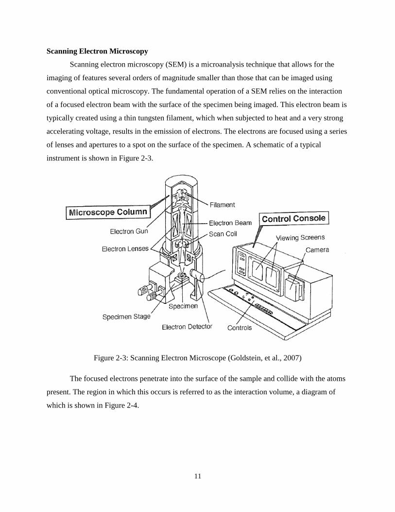
Scanning electron microscopy (SEM) is a microanalysis technique that allows for the
imaging of features several orders of magnitude smaller than those that can be imaged using
conventional optical microscopy. The fundamental operation of a SEM relies on the interaction
of a focused electron beam with the surface of the specimen being imaged. This electron beam is
typically created using a thin tungsten filament, which when subjected to heat and a very strong
accelerating voltage, results in the emission of electrons. The electrons are focused using a series
of lenses and apertures to a spot on the surface of the specimen. A schematic of a typical
instrument is shown in Figure 2-3.
Figure 2-3: Scanning Electron Microscope (Goldstein, et al., 2007)
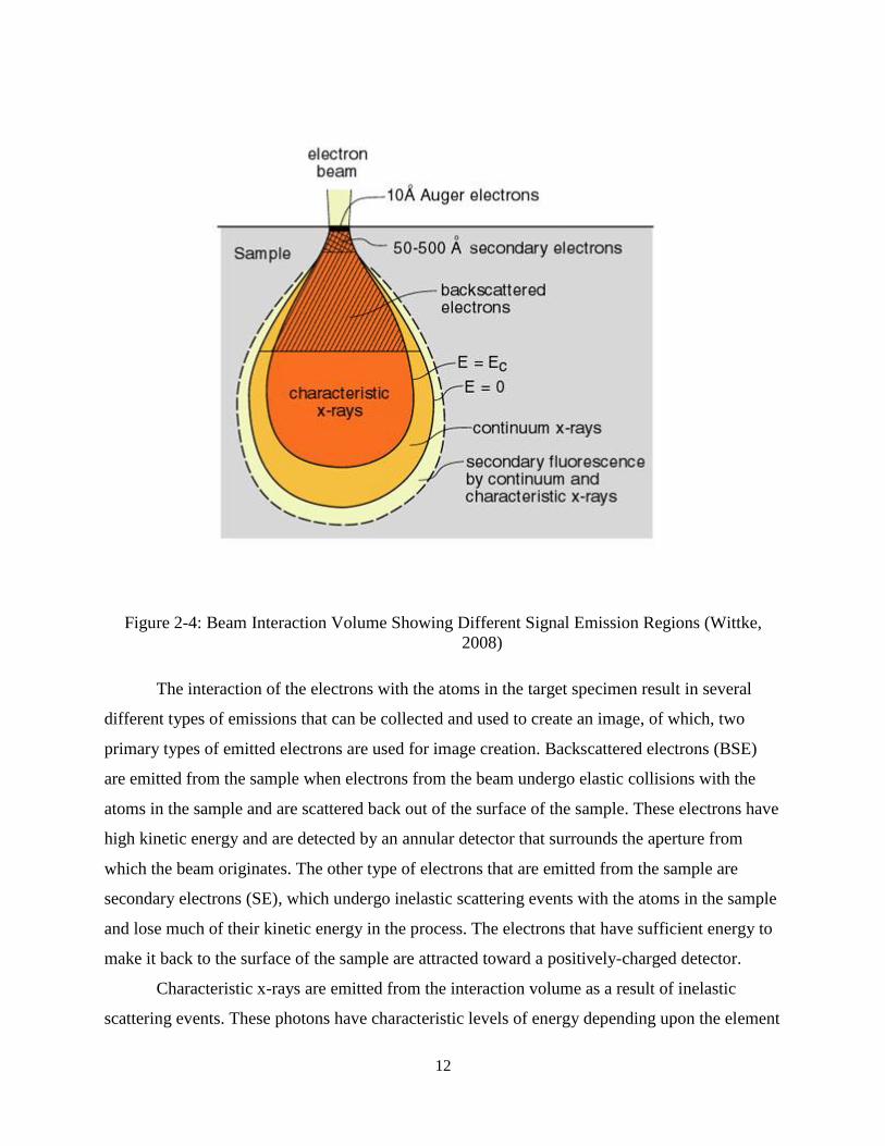
The focused electrons penetrate into the surface of the sample and collide with the atoms
present. The region in which this occurs is referred to as the interaction volume, a diagram of
which is shown in Figure 2-4.
12
Figure 2-4: Beam Interaction Volume Showing Different Signal Emission Regions (Wittke,
2008)
The interaction of the electrons with the atoms in the target specimen result in several
different types of emissions that can be collected and used to create an image, of which, two
primary types of emitted electrons are used for image creation. Backscattered electrons (BSE)
are emitted from the sample when electrons from the beam undergo elastic collisions with the
atoms in the sample and are scattered back out of the surface of the sample. These electrons have
high kinetic energy and are detected by an annular detector that surrounds the aperture from
which the beam originates. The other type of electrons that are emitted from the sample are
secondary electrons (SE), which undergo inelastic scattering events with the atoms in the sample
and lose much of their kinetic energy in the process. The electrons that have sufficient energy to
make it back to the surface of the sample are attracted toward a positively-charged detector.
Characteristic x-rays are emitted from the interaction volume as a result of inelastic
scattering events. These photons have characteristic levels of energy depending upon the element

13
with which they interact and enable the elemental analysis of a specimen, and this form of
imaging is referred to as energy dispersive x-ray spectroscopy or EDS.
The image in a SEM is produced by collecting the signal of interest from the target area,
and moving the electron beam rapidly in a grid pattern. Different signal intensities are created at
each spot (corresponding to a pixel) to produce contrast within the image. Contrast mechanisms
of the different imaging modes are the result of the physiochemical properties of the specimen.
BSEs are produced as a result of elastic scattering events, which occur more frequently in
specimens containing elements with relatively high atomic numbers. This results in an image in
which the brightest areas depict regions that have the highest average atomic number.
Topographic irregularities on the surface of the sample, which have exposed edges that provide
relatively short distances for secondary electrons to escape, appear brighter due to the larger
numbers of escaped secondary electrons. This “edge” effect enables relief or scratches in the
sample surface to be easily seen.
Though SEM allows for higher magnifications and different imaging modes than
conventional optical microscopy, certain aspects of the imaging process limit the types of
samples that can be imaged. The whole SEM is under vacuum, as gas would ionize in the
electron beam if present. This precludes the imaging of samples containing water or any other
compounds that would boil away at very low pressures. The sample must also either be
conductive or be made conductive, otherwise electrons will charge the surface of the specimen,
resulting in bright artifacts in the image. For elemental analysis using EDS, the sample must be
reasonably flat, as topographic variations can influence the degree to which x-rays are emitted
from different parts of the sample.
Computer Modeling
Since the invention of the transistor and the subsequent exponential growth of
computational processing power, efforts have been made to simulate complex systems through
the use of computer models. A model can be quite simply defined as a representation of a system
upon which operations can be performed to examine the response of the system to specific
stimuli. The engineering applications of computer modeling typically extend to numerical or
stochastic simulations, the former describing a system governed by equations that cannot be
solved analytically, and the latter describing a system where the occurrence of events is
probabilistic in nature. Both types of simulations have applications in civil engineering, with

14
numerical modeling of structural systems using the finite element method being most common,
while stochastic simulations are frequently applied to the simulation of weather phenomena.
The finite element method is a modeling technique used to numerically simulate the
overall behavior of geometrically complex objects by discretizing them into “elements” that are
interconnected, each of which can be described with its own set of equilibrium equations. Given
a certain set of “boundary conditions” which act on the geometry, the system of equations from
the individual elements can be solved to determine the influence of the boundary conditions on
the entire system (Zienkiewicz, et al., 2005). A common example of the application of this
method is the analysis of the deflection of a truss structure with pinned connections subjected to
specific loads. In the event the modeled structure remains in static equilibrium, the forces in each
discretized element of the structure must also be in equilibrium. Since the relationship between
force and displacement for each element is known, the system of equations for all elements can
be solved to find the resulting displacement of the structure as a whole.
Stochastic modeling is used to simulate the behavior of systems that are non-
deterministic, which means that they exhibit behavior that contains an element of randomness.
These systems can instead be described by the probabilities that events within the system will
occur. For example, the range of particle sizes that make up portland cement is highly variable.
Given a finite number of particles for a particular cement, the probability that a particle will be of
a particular size (the event) can be obtained by dividing the number of times that a particle, that
falls within a given size range, is observed, by the number of particles that are measured.

15
Figure 2-5: Particle Size Distribution
If all particles in a cement sample are measured and classified into different size ranges,
the frequency of occurrence of individual particles can be plotted for each size range creating the
distribution presented in Figure 2-5. The result is described as the probability density function
for the sizes of portland cement particles. This information can now be used to create a set of
virtual cement particles with the same distribution of sizes.
Cementitious Simulation
Background
The fundamental goal of modeling cementitious systems is to predict the physical and
durability properties of the material. Important structural-related properties of the hardened
cementitious microstructure modeled include hardened properties such as modulus of elasticity
and compressive strength, as well as durability-related properties such as porosity and
permeability. The creation of long-lasting concrete structures relies on the knowledge of these
characteristics of the material. The accurate determination of these properties via computer
simulation is dependent on the creation of a realistic virtual microstructure from which they can
be measured. Since the properties of the microstructure are dependent upon the composition and
hydration conditions of the cement from which it is created, there must also be a method by
which the development of the microstructure over time can be simulated.
0
1
2
3
4
5
6
7
8
9
0.1 1 10 100 1000
% M
easu
red
Par
ticl
es
Particle Diameter (µm)

16
History
The origins of cement microstructural modeling are from research performed in the
1970’s on the structure of amorphous semiconductors (Garboczi et al., 2000). Initial attempts to
calculate structural properties using approximate analytical solutions were only marginally
successful until a computer model was constructed consisting of several hundred randomly
linked atoms. Operations were performed on this model to calculate properties, and the resulting
properties were compared to experimental results. This model represented one of the first
attempts to model amorphous materials computationally at the atomic level.
The first attempt to model concrete computationally was recorded in the publication by
Wittmann, Roelfstra, and Sadouki in 1984 on the numerical simulation of the structure and
properties of concrete in two dimensions (Wittmann et al., 1984-1985). The two-dimensional
silhouettes of aggregates were first characterized by transforming the contour of an aggregate
particle section into polar coordinates. The radius of the particle as a function of the angle theta
about the y-axis could then be plotted, and the resulting frequency distribution obtained. The
frequency distributions of several particles of a given aggregate normalized for size were
combined to form a “morphological law” which was then used to generate aggregate sections
computationally.
17
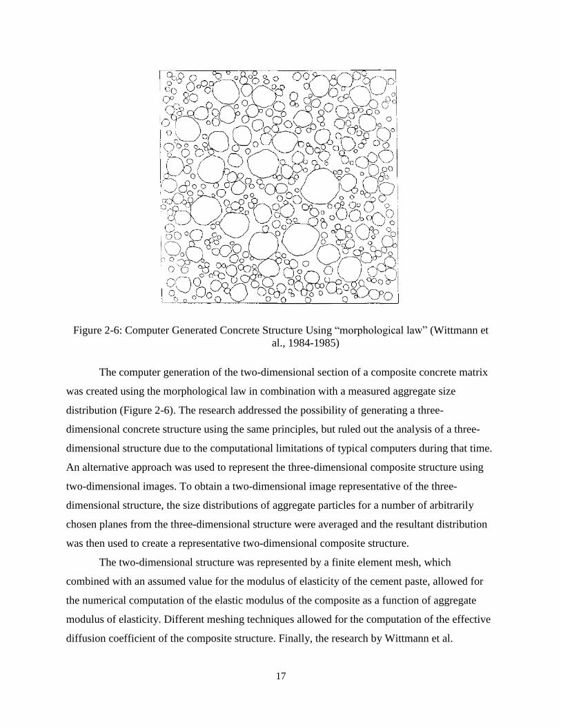
Figure 2-6: Computer Generated Concrete Structure Using “morphological law” (Wittmann et
al., 1984-1985)
The computer generation of the two-dimensional section of a composite concrete matrix
was created using the morphological law in combination with a measured aggregate size
distribution (Figure 2-6). The research addressed the possibility of generating a three-
dimensional concrete structure using the same principles, but ruled out the analysis of a three-
dimensional structure due to the computational limitations of typical computers during that time.
An alternative approach was used to represent the three-dimensional composite structure using
two-dimensional images. To obtain a two-dimensional image representative of the three-
dimensional structure, the size distributions of aggregate particles for a number of arbitrarily
chosen planes from the three-dimensional structure were averaged and the resultant distribution
was then used to create a representative two-dimensional composite structure.
The two-dimensional structure was represented by a finite element mesh, which
combined with an assumed value for the modulus of elasticity of the cement paste, allowed for
the numerical computation of the elastic modulus of the composite as a function of aggregate
modulus of elasticity. Different meshing techniques allowed for the computation of the effective
diffusion coefficient of the composite structure. Finally, the research by Wittmann et al.

18
concluded that further work could be done in which a mesh containing more detailed material
properties could be used to predict more complex behavior, such as creep, shrinkage, and non-
linear stress-strain behavior.
In 1986 the details of a three dimensional hydration model for C3S were published
(Jennings & Johnson, 1986). A model was created which followed rules based on measurable
characteristics of the system being simulated. The primary focus of this model was not to
accurately simulate the hydration behavior of C3S, but instead to provide a tool that connected
the probable mechanisms by which the reaction occurred with the measurable behavior of the
system. Such a tool is useful for the evaluation of the validity of a proposed mechanism by
simulating its effect on the behavior of the system.
The model simulated C3S particles as spheres, with the size distribution, number, and
initial packing type of the spheres entered by the user. Other user-controlled inputs included the
density of different hydration products, rules governing the distribution of hydration products,
and the rate-controlling reaction step at each stage. Simulations within the model began by
randomly distributing the specified number of particles with the specified size distribution.
Simulation of the cement hydration was initiated at the location of the smallest particle and
sequentially incremented. The diameter of the smallest particle was reduced by an amount that
was based on information known about the specified rate-controlling step. The space left by the
reduction in diameter was filled with hydration product surrounding the particle, and any
remaining hydration product was added to the diameter of the particle. This process was repeated
for each particle in sequence. One hydration cycle was complete when all particles had
undergone this process. The simulation continued until either all anhydrous phases were
consumed, the thickness of the hydrated product layer reached a user-specified value, or a
specific number of cycles were completed.
The resulting microstructure derived from simulations with this model was compared to
SEM micrographs of the hydrated C3S grains. A promising degree of resemblance was observed.
The future objectives of this research envisioned the use of the model for the evaluation of
different mechanical properties of the composite structure, and predicted the model would enable
research into proposed reaction mechanisms. The incorporation of the other phases of portland
cement was also envisioned.
19
This model was used as a tool for the simulation of cement hydration products for several
years, including work to apply a random walk algorithm for continuum models (including the
Jennings and Johnson model) in order to compute the electrical and diffusive transport properties
of the microstructure (Garboczi et al., 2000). This work introduced the idea of digitizing the
microstructure and experimented with a number of computations on a continuum-based
microstructure model. It was during this time that the advancements is computer technology
made it possible to create model simulations of sufficient size. The concept of a digital
microstructure is essentially a three-dimensional (3-D) image consisting of voxels (3-D pixels).
Each voxel represents a discrete volume of material with specific properties. A virtual
microstructure is created out of the voxels based on the physical and chemical characteristics of
the cement being modeled. Once the input parameters have been entered into the computer for
simulation, the virtual microstructure undergoes the simulated hydration process, with each
voxel acting as an independent agent. Voxels follow specific rules for dissolution, diffusion, and
reaction based on their phase and the known thermodynamic and kinetic behavior of cement
hydration. The creation of this digital microstructure led to the realization that nearly any finite
element or finite difference algorithm can be applied to measure the properties of the
microstructure. The only remaining steps were to establish the applications of percolation theory
and composite material theory to the digital microstructure.
The interconnected porosity in a cementitious body can be considered to be a system of
large pores, formed by the open interstices of particles in contact, that are connected by tortuous,
sheet- or capillary-like continuous spaces formed by close particle contact areas. The rate of
diffusion or fluid transport of material through the cementitious body is related to the volume of
the porosity, the tortuosity of the porosity, and the concentrations and concentration gradients of
the materials in the fluid. Percolation generally refers to the movement of a fluid through small
but interconnected porosity. However, when applied to the numerical modeling of a
cementitious s matrix, percolation theory is based on the connectivity of random phases in a
multiphase environment (Garboczi & Bentz, 1998).
There are two primary applications of the concept of percolation to the measureable
properties of a hydrating microstructure. The first is to model the degree of hydration of the
microstructure which is dependent on the extent with which reactants and reaction products can
diffuse throughout the microstructure through the water-filled capillary network. The ease of

20
transport is dependent on the size (equivalent diameter) and degree of interconnectedness (degree
of percolation) of the capillary network. As hydration progresses, the reactants and products
diffuse through the water-filled capillaries and deposit on the surfaces of the interconnected
capillary pathways, gradually reducing their size. The reduction in capillary size creates an
increase in tortuosity and a cementitious system with a lower rate of diffusion which ultimately
results in a reduced rate of transport. Thus, the degree of percolation of pore space at early ages
affects the extent and rate of initial hydration, and the progressive reduction in the rate of
diffusion reduces the progressive rate of hydration as the capillaries constrict.
The application of percolation theory to a digital lattice was established through work on
the conductivity of a plane containing random holes (Garboczi et al., 1991), and an algorithm
was developed to compute the linear elastic properties of a heterogeneous material from a digital
lattice a few years later (Garboczi & Day, 1995). The combination of different digital lattice-
based methods for the measurement of cement microstructure led to the eventual development in
1997 of a three-dimensional cement hydration model known as CEMHYD3D, the model, which
in an updated form, underpins the VCCTL software.
The VCCTL software was introduced by the National Institute for Standards and
Technology (NIST) in 2001 and was intended as a unified solution for modeling concrete at
multiple length scales. Concrete can be described as a multi-scale material, in that the properties
of the paste microstructure, which exist at a micro (10-6) scale, influence the properties of the
paste at a millimeter scale, which in turn influences the properties of the concrete at a macro-
scale level. The intention of the VCCTL software was to be a start-to-finish modeling solution
for concretes and mortars, requiring only data on the materials being simulated to provide
accurate measurements of mechanical and transport properties.
Validation of CEMHYD3D
CEMHYD3D, the hydration model used by the VCCTL software, has been available for
public use since 1997. There are a number of publications of note from this period, some of
which include a quantitative comparison of the initial and hydrated microstructures generated by
CEMHYD3D (Bentz 2005), and an investigation of the influence of ground limestone filler on
cement hydration (Bentz 2006). The research performed by Bentz, compared the simulated with
actual cement microstructures in an effort to investigate the validity of CEMHY3D for the
modeling of hydrating portland cement microstructures. Microstructures were compared visually
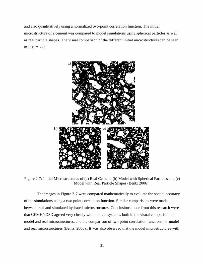
21
and also quantitatively using a normalized two-point correlation function. The initial
microstructure of a cement was compared to model simulations using spherical particles as well
as real particle shapes. The visual comparison of the different initial microstructures can be seen
in Figure 2-7.
Figure 2-7: Initial Microstructures of (a) Real Cement, (b) Model with Spherical Particles and (c)
Model with Real Particle Shapes (Bentz 2006)
The images in Figure 2-7 were compared mathematically to evaluate the spatial accuracy
of the simulations using a two point correlation function. Similar comparisons were made
between real and simulated hydrated microstructures. Conclusions made from this research were
that CEMHYD3D agreed very closely with the real systems, both in the visual comparison of
model and real microstructures, and the comparison of two-point correlation functions for model
and real microstructures (Bentz, 2006).. It was also observed that the model microstructures with
22
real particle shapes agree better with the two-point correlation functions of the real cement, and
that larger model system sizes also improve the agreement between these functions.
The investigation of the influence of finely ground limestone on the hydration of cement
(Bentz D. P., 2006) was triggered by a change in the ASTM C150 standard specification for
portland cement to allow for the inclusion of up to 5% of ground limestone, and the claim that
the presence of limestone does not influence the overall performance of portland cement.
CEMHYD3D was modified for this study to account for the hydration behavior of cements
containing ground limestone. The main modifications to the model accounted for the potential
for the additional surface area contributed by the limestone to provide more nucleation sites for
the growth of hydration products, as well as the potential for a chemical reaction to occur
between the cement and limestone itself. The results of the hydration model were validated
against experimental measurements of degree of hydration via non-evaporable water content.
This study concluded, based on good agreement of model and experimental data, that
CEMHYD3D successfully incorporated the chemical and surface area effects of ground
limestone.
Existing Research Using the VCCTL Software
The VCCTL software has been available for commercial and research use for over a
decade, and in that time has been continually developed and improved. Because of the continual
improvements made to the model during this time period, preference was given to more recent
research into the applications of the software. One of the simplest applications of the VCCTL
software is as an exploratory tool to investigate the effects of changes to cement chemistry. The
ability of the model to consider changes not only to cement composition but also fineness (via
particle size distributions) allows for optimization of the cement being produced with a minimum
of additional labor.
Work done by Siam Cement Group (SGC) (Sahachaiyunta, 2012) investigated the
influence of sulfate content and fineness on mortar strength. Twenty-five combinations of
fineness and sulfate content were simulated at 3, 7 and 28-day ages. The strength of the mortars
was calculated for all twenty-five combinations at different ages and used to evaluate the
performance of each permutation. It was concluded from results of plant trials that the VCCTL
software could be an effective tool for the optimization of different cement production

23
parameters, especially when considering more complex blended cements or the implementation
of high risk (economically) production strategies.
The VCCTL has great potential as an optimization tool for production within a cement
plant. Mapei Industries in conjunction with the University of Padua have performed some
successful validation studies using the VCCTL (Valentini, et al., 2013). The accuracy of both the
hydration simulation and modulus calculation of the software was evaluated for two different
cements. The experimental program consisted of the following:
In situ x-ray diffraction was used to measure the difference of volume fractions of
different cement phases and resultant hydration products over time.
Elastic modulus of mortar cubes was obtained and elastic modulus, compared to
the predictions / calculations by the VCCTL with respect to time.
Additionally, a power law equation was developed to empirically predict the
strength of mortars from elastic modulus.
Valentini et al. determined that the VCCTL software simulates the hydration behavior of
the chief hydration products, C-S-H and CH, and the diminishing quantity of C3S with a
reasonable degree of accuracy. However, there were substantial differences between the
measured and predicted volume fractions of ettringite within the system. This was attributed to
poor simulation by the VCCTL of the increased thermodynamic stability of ettringite in the
presence of carbonates. It was concluded that the inaccuracy would be largely irrelevant for the
prediction of mechanical properties, as ettringite made up less than 3% of the total volume of the
cementitious system. The study determined that there is relatively strong agreement between
prediction and measurement of elastic modulus and the empirical relationship developed for the
prediction of strength from modulus also correlated well with measurements. Of note is the
strong caution against the use of the empirical equation for strength developed in this study for
mortars in general, as the properties of the input materials may vary substantially.
Another current focus of research being conducted using the VCCTL software is the
characterization of the influence of addition of liquid admixtures. The software has the capacity
to integrate the influence of admixture additions into the system provided the behavior of the
admixture is known with respect to cement phase surface deactivation time, which is a parameter
that is not readily available for the majority of admixtures (Bullard & Obla, Virtual Testing of
Ready-Mixed Concrete, 2004). Previous research has examined the behavior of admixtures,

24
using gel permeation chromatography. Analysis of liquids obtained from filtering cement and
pure cement phase pastes enabled the measurement of the quantity of superplasticizer adsorbed
by the cement or constituent cement phase. The total quantity of plasticizer can be determined
based on the specific surface area of the cement particles obtained from Brunauer-Emmett-Teller
(BET) gas adsorption. This then allows for the determination of the duration of deactivation of
cement particle surfaces, which can then be entered directly into the VCCTL software (Russo,
2012). This technique is still in development, and has yet to be verified.
There is no research currently published that validates the accuracy of the VCCTL
software to predict the behavior of concrete as opposed to mortar. Studies do support the
accuracy of the software in the prediction of the properties of the cement paste as well as mortars
made with that paste (Bentz, 2006) (Valentini, et al., 2013) (Sahachaiyunta, 2012); however, the
methods by which the software incorporates coarse aggregate have yet to be systematically
validated.
Current Limitations of the VCCTL Software
Though the VCCTL software is the product of years of research into the modeling of
cementitious systems, there are still some aspects for which it is not robust. There is little
research which involves the simulation cementitious systems which include large percentages of
supplementary cementitious materials (SCMs) such as fly ash or ground granulated blast furnace
slag (slag). Fly ash and slag are products that are used in almost all concrete mixture designs
today. The Florida Department of Transportation, for instance, has a minimum fly ash
requirement for all structural concrete mixture designs. The software has some ability to handle
these materials; however, it has not been very well validated and is missing a number of details
as far at the thermodynamics and specifics of reactions are concerned (Garboczi, et al., 2010).
The VCCTL software has limited support for admixtures, and it is implemented in a way that
makes them difficult to implement into the simulation of cementitious systems. The model
requires that the specific amount of time that the surface of a phase is deactivated by the
admixture is known. This information is difficult to obtain and may only account for certain
aspects of admixture behavior. Efforts are currently underway to develop a process by which
admixtures can be characterized to obtain this information. It may also be possible to obtain this
information from the manufacturers of the admixtures themselves.
25
The long-term durability is one of the most important aspects of concrete, both for the
purposes of sustainability and economy and thus, a model that can predict the long-term
performance of concrete would benefit from some sort of durability prediction and degradation
modeling. Currently, the VCCTL software does not provide direct functionality for the
prediction of durability in concrete. The hydration model provides several outputs that can be
used for additional modeling to simulate the durability of concrete, however no direct outputs
currently exist.
Other Cementitious Modeling Software
The prediction of concrete performance is a problem for which a solution has great
economic potential. As a result, several commercial modeling solutions for concrete exist. None
of the models provide results that are based on the fundamental processes underpinning
cementitious systems, such as those simulated by the VCCTL software, but their more specific
focus has enabled viable alternatives.
The software model STADIUM is modeling software for cementitious systems that is
used to make service life predictions for concrete mixtures based on material testing. Thus, a
concrete mixture design being considered for use can be examined via physical testing and
compared to large databases of similar mix designs evaluated under different exposure
conditions. The model has been used for the prediction of service life for many different mixture
designs in many different environmental conditions, and has seen use by organizations such as
the US Navy. Though the service life predictions of STADIUM have reached a degree of
commercial acceptance, the models and databases from which it makes these predictions are
proprietary. The exact details of the function of STADIUM are not documented.
Mines ParisTech has produced a numerical model to simulate the effects of cracking and
alkali silicate reaction (ASR) in cementitious systems (Peyrot, 2006). The model uses a finite
element approach to simulate the growth of reactive aggregates bound in a cementitious matrix,
and the resulting bulk swelling. This model incorporates methods for simulating crack
development and propagation in heterogeneous materials. Though this direction of research is
promising, this model is still in the research stages, and has not seen any commercial use.
Another established concrete material model that has a somewhat different application is
TNO DIANA, a finite element model for reinforced concrete structures using realistic material
properties for concrete and steel. The software is capable of simulating cracking and crushing
26
failures, concrete-reinforcement interface zones, creep and shrinkage-induced cracking, material
aging effects, and thermally induced stresses. Work performed at the University of Florida
expanded the capability of the software to modeling of temperature rise in mass concrete
structures due to heat generated during cement hydration (Tia, et al., 2013). The use of heat of
hydration data obtained via isothermal calorimetry to build input files for TNO Diana enabled
the prediction of thermal stress distributions and cracking in mass concrete structures.
Comparison of the results of the simulations with real mass concrete structures found that the
prediction capability of the model was fair, with the model predicting higher temperatures than
those encountered in the field.
Currently, the Massachusetts Institute of Technology (MIT) Concrete Sustainability Hub
is working in cooperation with the Portland Cement Association (PCA) to create and model the
atomic structure of portland cement concrete. The goals of this Concrete Sustainability Hub are
to bring about breakthroughs in concrete science, and transfer those advancements to the
concrete industry (Who We Are, 2012). One of their key goals is the reduction of CO2 emissions
from portland cement production. Currently a number of advances in the understanding of the
nano-scale atomic structure of certain phases in cement have been realized, but a practical link
between any of these advances and the modeling of portland cement-based systems has not been
documented to date.
The specialized nature of these models differentiates them from the VCCTL software,
which is intended to be a full spectrum solution for the modeling of concrete. The further
development of the software to incorporate features such as fracture analysis and service life
prediction is ongoing.

27
CHAPTER 3 VCCTL SOFTWARE MATERIAL INPUTS
Overview
The most important part of using the VCCTL software is the proper characterization of
the materials being simulated. The model takes a number of different types of input data, some of
which are essential to running a simulation, and others which simply serve to enhance the
accuracy of simulations, or alter the way in which the virtual microstructure is generated or
hydrated. The inputs that are required for any hydration simulation include the following:
Cement phase volume and surface area fractions;
Cement phase relative spatial distributions;
Cement particle size distribution.
The following inputs are required to perform simulations including aggregates (mortar or
concrete),
Aggregate bulk and shear moduli;
Gradation of aggregate;
Specific gravity of aggregate.
There are other inputs that are not required by the VCCTL software to run simulations; however,
it is possible that the presence of these inputs may improve accuracy. For the purposes of this
research these inputs have been deemed “non-essential” and are as follows:
Heat of hydration curve of portland cement;
Mass fraction data of calcium sulfate phases present in cement;
Particle size distribution of sulfate phases;
Shape data of aggregate;
Shape data of cement particles;
Simulated microstructure size;
Particle dispersion of cement within microstructure.
The VCCTL software will accept and include data on the composition and particle size
distributions of pozzolanic materials such as fly ash or slag, as well as the chemical surface
deactivation behavior of admixtures. However, the investigation of these properties was out of
the scope of this research project.

28
Model Inputs for Portland Cement
Figure 3-1: Cement Input Screen of the VCCTL Software
The inputs required for portland cement can be divided into two categories: inputs that
are used to create the digital microstructure, and inputs used for the virtual hydration of the
cement microstructure. Many of these inputs can be obtained using the procedures as prescribed
in standardized testing methods and/or with specialized equipment, while others require more
complex analysis techniques and procedures. The cementitious material inputs are entered into
the VCCTL software through the Lab Materials – Cements page, shown in Figure 3-1.
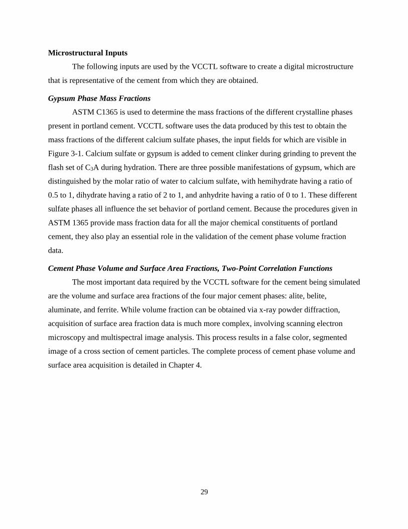
29
Microstructural Inputs
The following inputs are used by the VCCTL software to create a digital microstructure
that is representative of the cement from which they are obtained.
Gypsum Phase Mass Fractions
ASTM C1365 is used to determine the mass fractions of the different crystalline phases
present in portland cement. VCCTL software uses the data produced by this test to obtain the
mass fractions of the different calcium sulfate phases, the input fields for which are visible in
Figure 3-1. Calcium sulfate or gypsum is added to cement clinker during grinding to prevent the
flash set of C3A during hydration. There are three possible manifestations of gypsum, which are
distinguished by the molar ratio of water to calcium sulfate, with hemihydrate having a ratio of
0.5 to 1, dihydrate having a ratio of 2 to 1, and anhydrite having a ratio of 0 to 1. These different
sulfate phases all influence the set behavior of portland cement. Because the procedures given in
ASTM 1365 provide mass fraction data for all the major chemical constituents of portland
cement, they also play an essential role in the validation of the cement phase volume fraction
data.
Cement Phase Volume and Surface Area Fractions, Two-Point Correlation Functions
The most important data required by the VCCTL software for the cement being simulated
are the volume and surface area fractions of the four major cement phases: alite, belite,
aluminate, and ferrite. While volume fraction can be obtained via x-ray powder diffraction,
acquisition of surface area fraction data is much more complex, involving scanning electron
microscopy and multispectral image analysis. This process results in a false color, segmented
image of a cross section of cement particles. The complete process of cement phase volume and
surface area acquisition is detailed in Chapter 4.
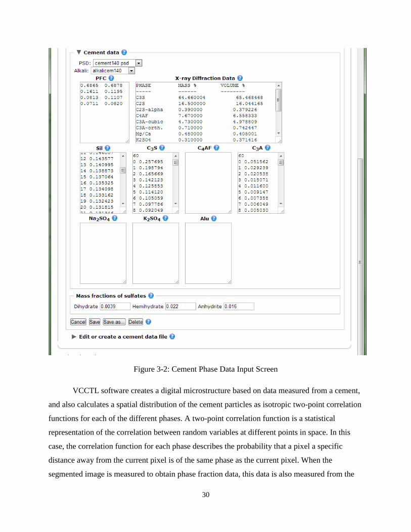
30
Figure 3-2: Cement Phase Data Input Screen
VCCTL software creates a digital microstructure based on data measured from a cement,
and also calculates a spatial distribution of the cement particles as isotropic two-point correlation
functions for each of the different phases. A two-point correlation function is a statistical
representation of the correlation between random variables at different points in space. In this
case, the correlation function for each phase describes the probability that a pixel a specific
distance away from the current pixel is of the same phase as the current pixel. When the
segmented image is measured to obtain phase fraction data, this data is also measured from the
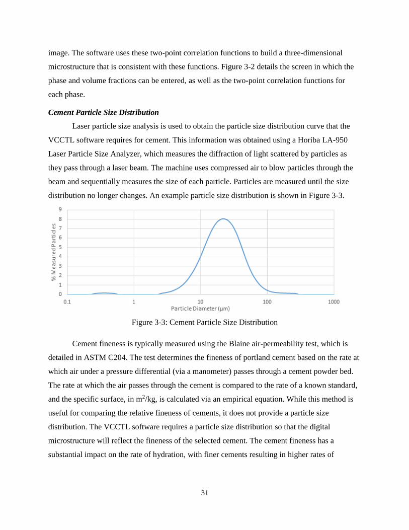
31
image. The software uses these two-point correlation functions to build a three-dimensional
microstructure that is consistent with these functions. Figure 3-2 details the screen in which the
phase and volume fractions can be entered, as well as the two-point correlation functions for
each phase.
Cement Particle Size Distribution
Laser particle size analysis is used to obtain the particle size distribution curve that the
VCCTL software requires for cement. This information was obtained using a Horiba LA-950
Laser Particle Size Analyzer, which measures the diffraction of light scattered by particles as
they pass through a laser beam. The machine uses compressed air to blow particles through the
beam and sequentially measures the size of each particle. Particles are measured until the size
distribution no longer changes. An example particle size distribution is shown in Figure 3-3.
Figure 3-3: Cement Particle Size Distribution
Cement fineness is typically measured using the Blaine air-permeability test, which is
detailed in ASTM C204. The test determines the fineness of portland cement based on the rate at
which air under a pressure differential (via a manometer) passes through a cement powder bed.
The rate at which the air passes through the cement is compared to the rate of a known standard,
and the specific surface, in m2/kg, is calculated via an empirical equation. While this method is
useful for comparing the relative fineness of cements, it does not provide a particle size
distribution. The VCCTL software requires a particle size distribution so that the digital
microstructure will reflect the fineness of the selected cement. The cement fineness has a
substantial impact on the rate of hydration, with finer cements resulting in higher rates of
32
hydration (Mindess & Young, 1981). This input is also selected on the screen shown in Figure 3-
2.
Figure 3-4: Microstructure Simulation Parameters
Cement Particle Shape Data
The VCCTL software builds the digital microstructure using spherical particles, though it
also has provisions for the use of real cement particle shapes. These particle shapes are obtained
using x-ray computed microtomography scans of real cement particles, which are then
individually modeled using a spherical harmonic expansion of the particle surface. The
coefficients of the equations used to model the particle can then be used to reconstruct the
particle virtually with arbitrary size and orientation (Bullard & Garboczi, 2006). No cements
were characterized in this way during this research; however, the software contains a library of
cement particle shape sets. A cement from the library with particle shapes judged to be similar to
that of the cement used in this research was used when simulations with real particle shapes were
run. A screenshot showing this option is visible in Figure 3-4
Cement Particle Dispersion
The VCCTL software provides the option to create a simulation that considers dispersed
cement particles as it composes the virtual microstructure. This option is provided to simulate the
mutual repulsion of cement particles that occurs (Mamlouk & Zaniewski, 2010) when water-

33
reducing admixtures are present. The functional effect of this is that space between particles is
more uniform, which can result in more accurate simulation of hydration and a corresponding
increase in strength (Neville, 2011). When simulating mixes with water-reducing admixtures,
this option (shown in Figure 3-4) was enabled and set to a value of one. The dispersion of
particles can be set to 0, 1, or 2, with the values indicating the minimum number of pixels
separating each particle in the virtual microstructure.
Binder System Size
By default, the volume of the microstructure created by the VCCTL software is 100
microns cubed. The size of the microstructure can be increased or decreased by the user, though
a linear increase in the side of the virtual microstructure will result in a cubic increase in volume,
impacting the time required for the computer modeling of microstructure operations.
Hydration Modeling Inputs
The following inputs are used by the VCCTL software to govern the behavior of the
hydrating microstructure.
Isothermal Conduction Calorimetry – ASTM C1702
ASTM C1702 details a standard test method for the measurement of heat of hydration of
hydraulic cementitious materials using isothermal conduction calorimetry, a process which has
seen widespread adoption for cementitious research in the last few decades (Ferraro, 2009). The
method details the construction and function of an isothermal conduction calorimeter, the
recommended procedures for the preparation of samples, and explains the analysis of the results
obtained from a calorimeter to determine heat of hydration. The test method defines an
isothermal conduction calorimeter as a constant temperature heat sink to which two heat flux
sensors and sample holders are attached in a manner that insures good thermal conductivity. The
two sample holders are required for the analysis of one sample, one for the cementitious sample
and one for a reference sample that evolves no heat.
The heat of hydration evolved by the sample flows across the heat sensor and into the
heat sink. The measured heat of hydration is the difference between the heat flow of the sample
cell and the reference cell. A schematic diagram of a basic isothermal calorimeter is shown in
Figure 3-5 (ASTM C1702, 2009).

34
Figure 3-5: Simple Isothermal Calorimeter (ASTM C1702, 2009).
One of the defining characteristics of hydraulic cements is that they exhibit an
exothermic reaction when mixed with water. Ideally, the heat released from this reaction should
be measured from the moment the sample is mixed with water and sample the should be in
thermal equilibrium with the environment within the calorimeter, as any heat flow through the
sensor that exists prior to hydration can distort the measurements acquired. The standardized test
method details a procedure by which these two conditions can be met and is referred to as
internal mixing.
An admix ampoule, shown mounted onto a sample vial in Figure 3-6, is used to facilitate
internal mixing. The admix ampoule has an o-ring seal, syringes that hold the mix water, and a
mechanical stirrer for mixing. The admix ampoule-sample vial assembly is placed inside the
isothermal calorimeter and allowed to reach thermal equilibrium prior to mixing. After
equilibrium is reached, the water is ejected from the syringes into the sample vial containing the
cementitious material, and the paste is mixed using the manual stirrer. The total heat evolved is
typically recorded for 7 days.
The specification also outlines an alternative method for sample mixing, in which the
sample is mixed outside the calorimeter and immediately inserted and measured. While much
simpler than the previous procedure to execute, the test specification acknowledges a few
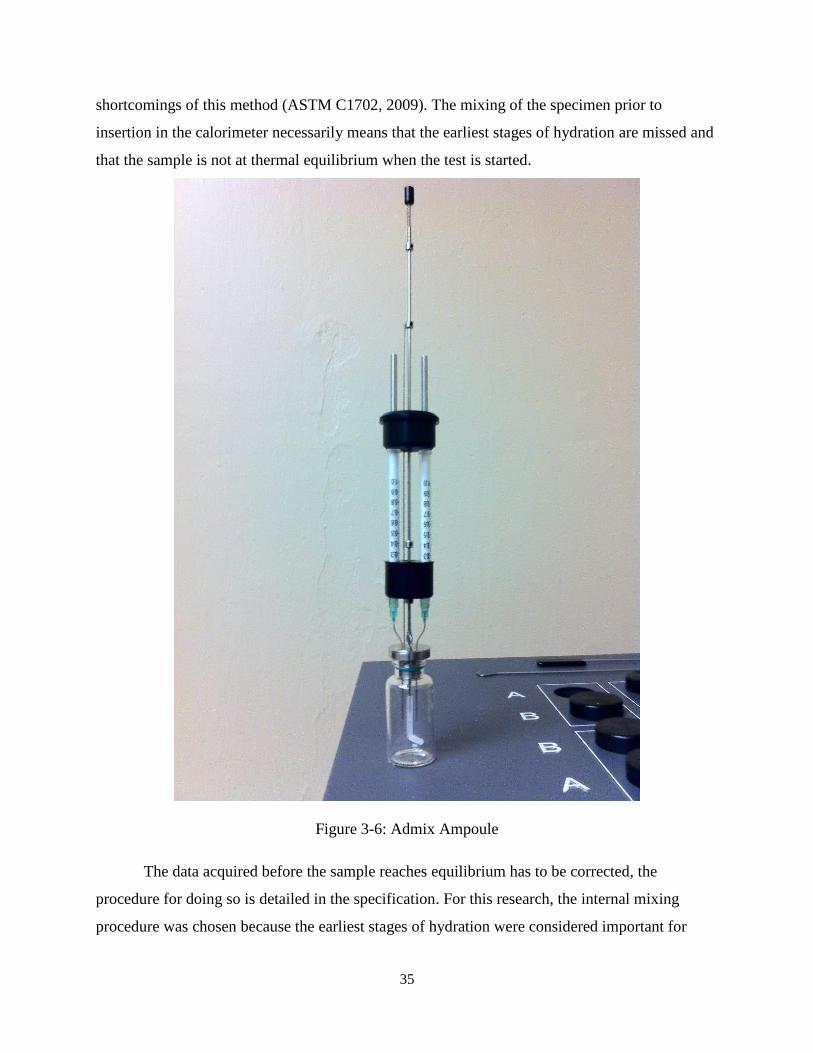
35
shortcomings of this method (ASTM C1702, 2009). The mixing of the specimen prior to
insertion in the calorimeter necessarily means that the earliest stages of hydration are missed and
that the sample is not at thermal equilibrium when the test is started.
Figure 3-6: Admix Ampoule
The data acquired before the sample reaches equilibrium has to be corrected, the
procedure for doing so is detailed in the specification. For this research, the internal mixing
procedure was chosen because the earliest stages of hydration were considered important for

36
evaluating the effects of admixtures, the acknowledged shortcomings of the external mixing
procedure in the test specification, and past research showing the viability of the internal mixing
procedure (Ferraro, 2009).
The specific sample preparation procedure used for isothermal calorimetry analysis was
as follows. The quantities of cement and water to be used were calculated such that the total heat
capacity of cement and water together were equal to that of the reference (inert) specimen. The
cement was then carefully introduced to the sample vial, while monitoring the mass on a research
balance, until the desired mass was reached. Deionized water was carefully drawn into the admix
ampoule and measured on the balance. The process was repeated until the desired mass of water
was contained in the syringes. Afterwards, a small amount of air was drawn into the tips of the
syringes to help prevent drops of water from leaking onto the cementitious material while the
sample was reaching thermal equilibrium within the isothermal calorimeter. Vials and admix
ampoules were assembled with a small amount of vacuum grease to seal connections and then
inserted into the calorimeter. At least three companion specimens for each mixture were used,
with two mixes measured during one 7-day test period.
Figure 3-7: Tam Air Isothermal Calorimeter with Sample and Admix Ampoule Loaded

37
For this research a TAM Air isothermal calorimeter was used, shown in Figure 3-7. The
calorimeter consisted of 8 channels, each channel consisting of two cells in the configuration
shown in Figure 3-7. Samples were allowed to equilibrate for at least 12 hours overnight.
Measurements began for each sample when the water was injected into the sample vial. Samples
were stirred manually for 60 seconds each, after which measurements were taken for seven days.
Figure 3-8: Hydration Simulation Input Parameters
The resulting power curve for the seven-day hydration reaction can be integrated over
time to obtain a heat of hydration curve, which in turn can be input directly into the VCCTL

38
software as a text file. The input screen for the selection of a heat of hydration curve can be seen
in Figure 3-8. For each computational cycle of the hydration reaction, the software calculates the
amount of heat released. Heat of hydration data is not required by the software for hydration
simulations, as the model assigns the same length (user input) to each cycle; however, if the
experimentally measured heat of hydration data (via ASTM C1702) is entered into the software,
the model will assign a length to each computational cycle of the simulation such that the heat
evolved during that cycle matches up with the input heat of hydration curve.
Curing Conditions
The VCCTL software provides input options to simulate different possible curing
conditions for the hydrating microstructure, shown in Figure 3-8. The “Thermal” condition
options regulate the rate at which the heat evolved during hydration leaves the microstructure.
The “Isothermal” thermal condition selection sets the rate to be equal to the rate at which heat is
evolved (keeping the microstructure at ambient temperature), the “Semi-Adiabatic” option sets
the rate at a user-specified value, and the “Adiabatic” option sets the rate such that no heat leaves
the microstructure.
The options for “Saturation conditions” influence the water available for the hydration
simulation. The saturated option allows the microstructure to never run out of water for
hydration reactions, while the sealed option limits the available water to that which is in the
initial microstructure. For the purposes of this research, the saturated option was always selected.
Data Output
The VCCTL allows the user to specify the intervals at which specific types of
data are measured from the hydrating microstructure, including the degree to which the pore
space in the microstructure is interconnected (percolation of porosity), the degree to which the
solids in the microstructure are interconnected (percolation of total solids) and the degree to
which each particle within the microstructure is hydrated. These options are shown in Figure 3-8,
and are computed at user specified intervals. Also part of the data output section are the intervals
at which to output microstructures for moduli calculations.

39
Aggregate Input Data
Most of the input data required by the VCCTL software for aggregates come from ASTM
standard tests that are performed on aggregates as a matter of course, the results of which are
readily available. A brief summary of these tests follows:
ASTM C136 – Standard Test Method for the Sieve Analysis of Fine and Coarse
Aggregate. This test is run on all aggregates used at the FDOT;
ASTM C127 – Standard Test Method for Density, Relative Density (Specific
Gravity), and Absorption of Coarse Aggregate. This test is also run for all aggregates
used at the FDOT.
The primary use of the aggregate input data by the software is simply to convert the mass
fractions to volume fractions when batching the virtual mix. Aggregate bulk and shear moduli
are not among the data readily available to characterize aggregate. While the aggregate
properties can be measured from rock cores sourced from the mine where the aggregate
originated, there is a degree of inherent variability to natural aggregate that makes obtaining
representative cores difficult. This process was not performed for this research due to time and
scope constraints. Instead, some values were assumed for the coarse and fine aggregate used in
this study based on the knowledge that the VCCTL software requires this data for the calculation
of the modulus of concrete. As concrete is mostly aggregate by volume, bulk and shear moduli
potentially have a substantial influence on the results. Thus, future research should include a
detailed investigation of these properties.
The VCCTL software accounts for aggregate shape data as a statistical distribution of
spherical harmonic coefficients, which is obtained via x-ray computed tomography. The software
includes shape data for a variety of aggregates in its built-in library of materials, and the
influence of aggregate shape on simulation results was investigated as part of this study and is
discussed in Chapter 7.

40
CHAPTER 4 SEM MICROANALYSIS
Overview
The phase volume fractions and surface area fractions are required inputs for VCCTL
software to simulate cement microstructure as it hydrates, and are acquired via a combination of
scanning electron microscopy and image analysis. The process was orginally developed at NIST
and consists of three primary operations.
1. Backscatter Electron and X-Ray Map Image Acquisition,
2. Image Processing, and
3. Creation and Analysis of Segmented Image.
Before any of the data acquisition operations can take place a significant amount of sample
preparation is required to enable the imaging of the cement being analyzed within the scanning
electron microscope.
Sample Preparation
Procedures Developed by NIST
The phase volume and surface area fraction data required by the VCCTL software is
obtained through a complex process involving image acquisition using a scanning electron
microscope (SEM). Before this process can even begin however, the cement being analyzed
must be prepared so that imaging is possible. The analysis process examines cross sections of
cement grains which must be flat and very smooth, free of scratches, tear outs, and other
imperfections that could skew measurement or cause imaging artifacts. The process required to
achieve this is complex and sensitive. The original procedure for the preparation of cement
powder specimens for imaging in this way was developed by NIST to provide inputs for
different cement hydration models. This original process, outlined in the next few paragraphs,
was used as a starting point for the procedure developed for this project.
The cement is first mixed with an optical grade epoxy resin in proportions that result in a
stiff paste. The paste is then formed into a ball and pressed into a specimen mold. The paste is
consolidated by tapping the mold sharply upon the table top. Once consolidation is complete, the
specimen is then cured according to the guidelines recommended by the epoxy manufacturer.

41
After the specimen is cured, a fresh surface is exposed by grinding or sectioning with a wafering
saw.
Following the resin encapsulation process, the specimen is ground with silicon carbide
sandpaper using progressively finer abrasives, stopping at 600 grit. This process serves to
remove the damage to the surface left by the diamond saw blade, and prepares the surface for the
final polishing steps. The specimen is polished using progressively finer grit diamond abrasive
and a polishing cloth, specifically 6, 3, 1, and 0.25 µm. At each stage the specimen is polished
until the imperfections left from the preceding abrasive are removed. Ethanol-based lubricants
are used throughout the cutting, grinding, and polishing process in order to prevent further
hydration of the cement grains or paste. The final polished surface is carefully cleaned, after
which a carbon coating is applied to render the sample conductive for imaging in the SEM.
Improvements to Sample Preparation
The original procedure developed by NIST was almost 20 years old when this research
project began. Though the fundamental process remains the same, substantial improvements to
the speed of preparation and consistency of quality were made. One of the biggest improvements
made to the existing procedure was the automation of the grinding and polishing operations. The
original process involved hand grinding of samples using silicon carbide paper on plates of glass,
followed by hand polishing using a manual lapping wheel. These operations are very labor
intensive and require a considerable degree of operator skill.
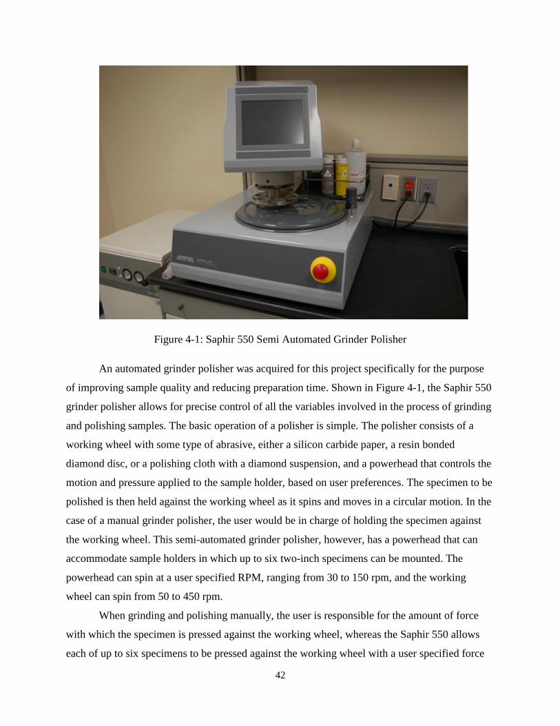
42
Figure 4-1: Saphir 550 Semi Automated Grinder Polisher
An automated grinder polisher was acquired for this project specifically for the purpose
of improving sample quality and reducing preparation time. Shown in Figure 4-1, the Saphir 550
grinder polisher allows for precise control of all the variables involved in the process of grinding
and polishing samples. The basic operation of a polisher is simple. The polisher consists of a
working wheel with some type of abrasive, either a silicon carbide paper, a resin bonded
diamond disc, or a polishing cloth with a diamond suspension, and a powerhead that controls the
motion and pressure applied to the sample holder, based on user preferences. The specimen to be
polished is then held against the working wheel as it spins and moves in a circular motion. In the
case of a manual grinder polisher, the user would be in charge of holding the specimen against
the working wheel. This semi-automated grinder polisher, however, has a powerhead that can
accommodate sample holders in which up to six two-inch specimens can be mounted. The
powerhead can spin at a user specified RPM, ranging from 30 to 150 rpm, and the working
wheel can spin from 50 to 450 rpm.
When grinding and polishing manually, the user is responsible for the amount of force
with which the specimen is pressed against the working wheel, whereas the Saphir 550 allows
each of up to six specimens to be pressed against the working wheel with a user specified force
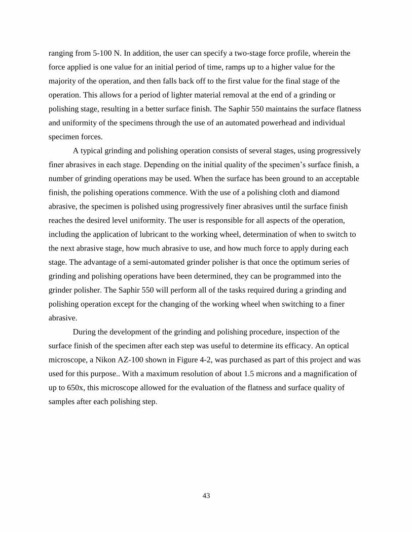
43
ranging from 5-100 N. In addition, the user can specify a two-stage force profile, wherein the
force applied is one value for an initial period of time, ramps up to a higher value for the
majority of the operation, and then falls back off to the first value for the final stage of the
operation. This allows for a period of lighter material removal at the end of a grinding or
polishing stage, resulting in a better surface finish. The Saphir 550 maintains the surface flatness
and uniformity of the specimens through the use of an automated powerhead and individual
specimen forces.
A typical grinding and polishing operation consists of several stages, using progressively
finer abrasives in each stage. Depending on the initial quality of the specimen’s surface finish, a
number of grinding operations may be used. When the surface has been ground to an acceptable
finish, the polishing operations commence. With the use of a polishing cloth and diamond
abrasive, the specimen is polished using progressively finer abrasives until the surface finish
reaches the desired level uniformity. The user is responsible for all aspects of the operation,
including the application of lubricant to the working wheel, determination of when to switch to
the next abrasive stage, how much abrasive to use, and how much force to apply during each
stage. The advantage of a semi-automated grinder polisher is that once the optimum series of
grinding and polishing operations have been determined, they can be programmed into the
grinder polisher. The Saphir 550 will perform all of the tasks required during a grinding and
polishing operation except for the changing of the working wheel when switching to a finer
abrasive.
During the development of the grinding and polishing procedure, inspection of the
surface finish of the specimen after each step was useful to determine its efficacy. An optical
microscope, a Nikon AZ-100 shown in Figure 4-2, was purchased as part of this project and was
used for this purpose.. With a maximum resolution of about 1.5 microns and a magnification of
up to 650x, this microscope allowed for the evaluation of the flatness and surface quality of
samples after each polishing step.
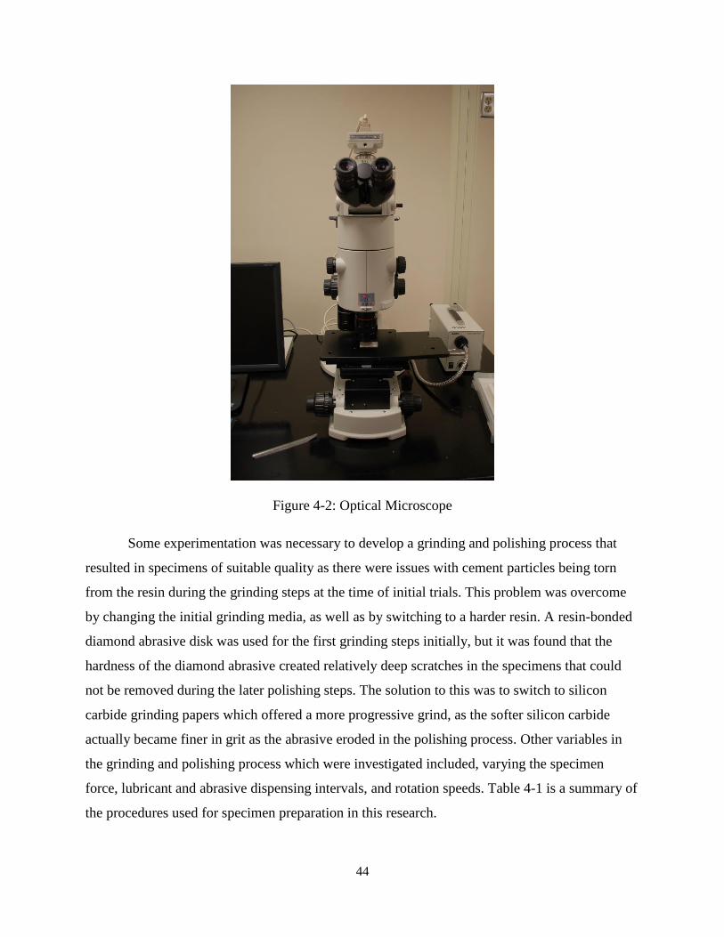
44
Figure 4-2: Optical Microscope
Some experimentation was necessary to develop a grinding and polishing process that
resulted in specimens of suitable quality as there were issues with cement particles being torn
from the resin during the grinding steps at the time of initial trials. This problem was overcome
by changing the initial grinding media, as well as by switching to a harder resin. A resin-bonded
diamond abrasive disk was used for the first grinding steps initially, but it was found that the
hardness of the diamond abrasive created relatively deep scratches in the specimens that could
not be removed during the later polishing steps. The solution to this was to switch to silicon
carbide grinding papers which offered a more progressive grind, as the softer silicon carbide
actually became finer in grit as the abrasive eroded in the polishing process. Other variables in
the grinding and polishing process which were investigated included, varying the specimen
force, lubricant and abrasive dispensing intervals, and rotation speeds. Table 4-1 is a summary of
the procedures used for specimen preparation in this research.
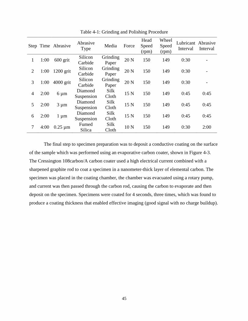
45
Table 4-1: Grinding and Polishing Procedure
The final step to specimen preparation was to deposit a conductive coating on the surface
of the sample which was performed using an evaporative carbon coater, shown in Figure 4-3.
The Cressington 108carbon/A carbon coater used a high electrical current combined with a
sharpened graphite rod to coat a specimen in a nanometer-thick layer of elemental carbon. The
specimen was placed in the coating chamber, the chamber was evacuated using a rotary pump,
and current was then passed through the carbon rod, causing the carbon to evaporate and then
deposit on the specimen. Specimens were coated for 4 seconds, three times, which was found to
produce a coating thickness that enabled effective imaging (good signal with no charge buildup).
Step Time Abrasive Abrasive
Type Media Force
Head
Speed
(rpm)
Wheel
Speed
(rpm)
Lubricant
Interval
Abrasive
Interval
1 1:00 600 grit Silicon
Carbide
Grinding
Paper 20 N 150 149 0:30 -
2 1:00 1200 grit Silicon
Carbide
Grinding
Paper 20 N 150 149 0:30 -
3 1:00 4000 grit Silicon
Carbide
Grinding
Paper 20 N 150 149 0:30 -
4 2:00 6 µm Diamond
Suspension
Silk
Cloth 15 N 150 149 0:45 0:45
5 2:00 3 µm Diamond
Suspension
Silk
Cloth 15 N 150 149 0:45 0:45
6 2:00 1 µm Diamond
Suspension
Silk
Cloth 15 N 150 149 0:45 0:45
7 4:00 0.25 µm Fumed
Silica
Silk
Cloth 10 N 150 149 0:30 2:00

46
Figure 4-3: Evaporative Carbon Coater
Backscattered Electron and X-Ray Map Image Acquisition
After the completion of the sample preparation process, an unhydrated cement sample
was analyzed using a scanning electron microscope. The two primary imaging modes used in
this process were backscattered electron (BSE) and energy dispersive x-ray (EDS) mapping. The
BSE mode created an image wherein the contrast was determined by the relative average atomic
number (Z) of the different phases, with the brightest phases having the highest average atomic
number. A typical BSE image is presented in Figure 4-4. The brightest phase present is the
ferrite phase (C4AF), due to the presence of iron, with is denser relative to the other phases,
which are composed of mainly calcium, aluminum, and silicon. The darkest phase is the epoxy
substrate, as it is a plastic and thus composed primarily of relatively low-atomic number carbon
polymer chains. The phases in order of darkest to lightest (lowest to highest atomic number) are
the voids (epoxy-filled), gypsum, C3A, C2S, C3S, and C4AF.

47
Figure 4-4: Cement Grain Close-up at 1600x magnification
Figure 4-4 is a close-up of a polished cement grain. It is possible to discern the four
primary cement phases with a reasonable degree of accuracy based on the relative grey levels
and the morphology of the phases (aluminate is typically dispersed within ferrite, for instance).
However, computerized quantitative analysis of the area and perimeter of each phase was not
possible without more information, as different phases (belite and aluminate) had overlapping
ranges of grey values. BSE images used for analysis were typically of a larger area than that
shown in Figure 4-4. An example of a typical image used for this process is provided in Figure
4-5.
The second imaging mode needed for this technique, EDS, was used to create an image
that showed the location and relative concentration of specific elements within the cement
sample. Elements can be identified due to the characteristic nature of the electron beam-

48
Figure 4-5: BSE Image as Used for Phase Analysis, 800x Magnification
specimen interactions, where the number of interactions for a particular element determines the
relative brightness (elemental contrast) in a backscattered SEM image, and is related to the
atomic number of the element. The interaction of the electron beam with the electron clouds of
atoms in the specimen results in the ejection of inner-shell electrons which result in higher-
energy outer-shell electrons moving to empty lower-energy inner shells, which results in the
release of x-ray photons. The photons have energies equal to the differences in the energy states
of the donor and recipient orbitals in the affected atoms. These photon energies uniquely identify
the corresponding elements and are referred to as characteristic energies. By scanning a selected
area of the specimen for x-ray photons of a specific energy, a “map” is created for the particular
element identified by the characteristic energy.

49
Figure 4-6: Elemental Map for Sulfur
An example of an EDS elemental map of the region shown in Figure 4-5 is presented in
Figure 4-6. The areas that are not black denote the presence of sulfur. This sulfur map and
corresponding maps for aluminum, sodium, and potassium, provide the additional information
needed to distinguish the phases present in the BSE image that would otherwise be partially
indistinguishable due to overlapping grey values.
Figure 4-7: BSE, Sulfur, and Aluminum Maps Required to Distinguish Alite, Belite, Aluminate,
Ferrite, and Gypsum
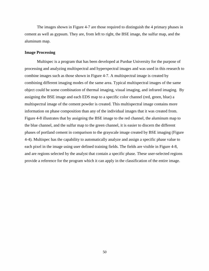
50
The images shown in Figure 4-7 are those required to distinguish the 4 primary phases in
cement as well as gypsum. They are, from left to right, the BSE image, the sulfur map, and the
aluminum map.
Image Processing
Multispec is a program that has been developed at Purdue University for the purpose of
processing and analyzing multispectral and hyperspectral images and was used in this research to
combine images such as those shown in Figure 4-7. A multispectral image is created by
combining different imaging modes of the same area. Typical multispectral images of the same
object could be some combination of thermal imaging, visual imaging, and infrared imaging. By
assigning the BSE image and each EDS map to a specific color channel (red, green, blue) a
multispectral image of the cement powder is created. This multispectral image contains more
information on phase composition than any of the individual images that it was created from.
Figure 4-8 illustrates that by assigning the BSE image to the red channel, the aluminum map to
the blue channel, and the sulfur map to the green channel, it is easier to discern the different
phases of portland cement in comparison to the grayscale image created by BSE imaging (Figure
4-4). Multispec has the capability to automatically analyze and assign a specific phase value to
each pixel in the image using user defined training fields. The fields are visible in Figure 4-8,
and are regions selected by the analyst that contain a specific phase. These user-selected regions
provide a reference for the program which it can apply in the classification of the entire image.
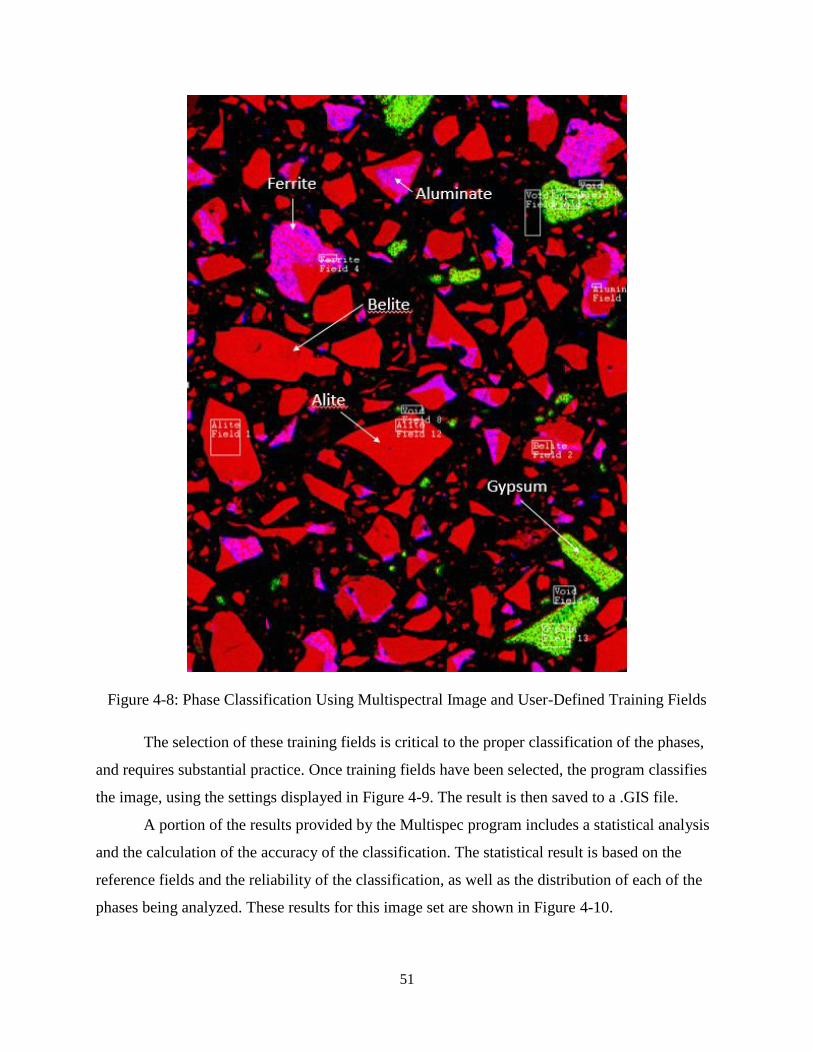
51
Figure 4-8: Phase Classification Using Multispectral Image and User-Defined Training Fields
The selection of these training fields is critical to the proper classification of the phases,
and requires substantial practice. Once training fields have been selected, the program classifies
the image, using the settings displayed in Figure 4-9. The result is then saved to a .GIS file.
A portion of the results provided by the Multispec program includes a statistical analysis
and the calculation of the accuracy of the classification. The statistical result is based on the
reference fields and the reliability of the classification, as well as the distribution of each of the
phases being analyzed. These results for this image set are shown in Figure 4-10.
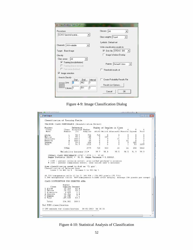
52
Figure 4-9: Image Classification Dialog
Figure 4-10: Statistical Analysis of Classification
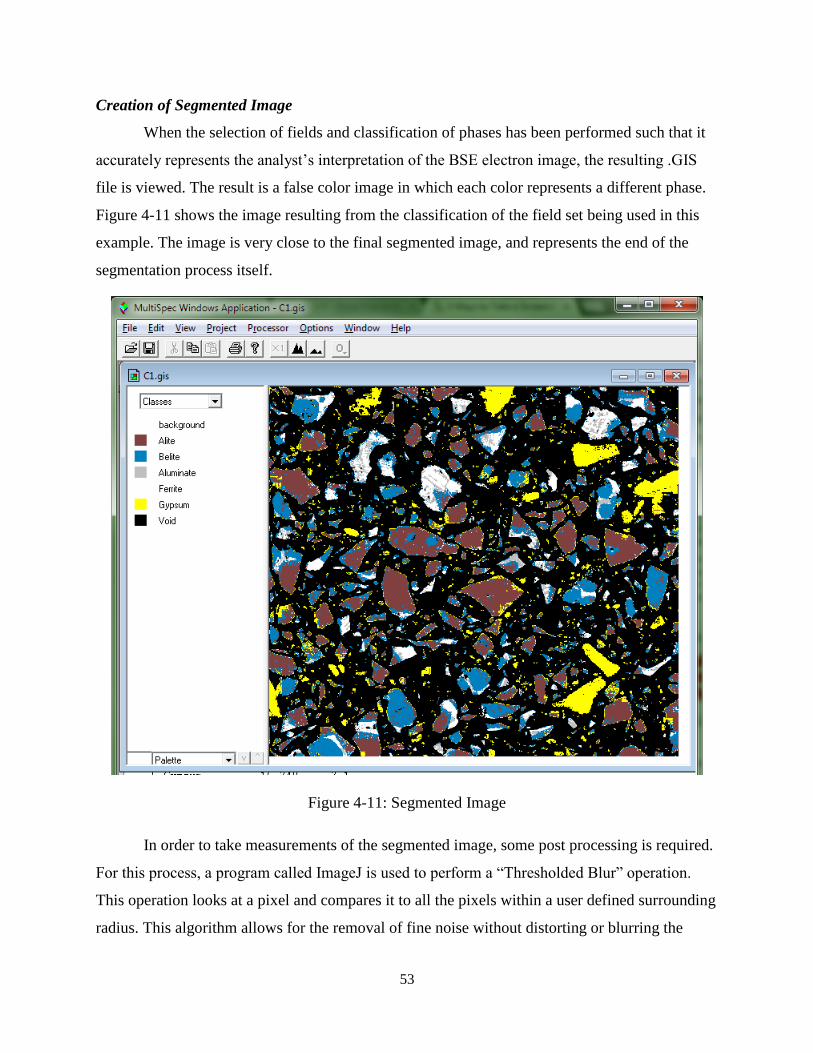
53
Creation of Segmented Image
When the selection of fields and classification of phases has been performed such that it
accurately represents the analyst’s interpretation of the BSE electron image, the resulting .GIS
file is viewed. The result is a false color image in which each color represents a different phase.
Figure 4-11 shows the image resulting from the classification of the field set being used in this
example. The image is very close to the final segmented image, and represents the end of the
segmentation process itself.
Figure 4-11: Segmented Image
In order to take measurements of the segmented image, some post processing is required.
For this process, a program called ImageJ is used to perform a “Thresholded Blur” operation.
This operation looks at a pixel and compares it to all the pixels within a user defined surrounding
radius. This algorithm allows for the removal of fine noise without distorting or blurring the
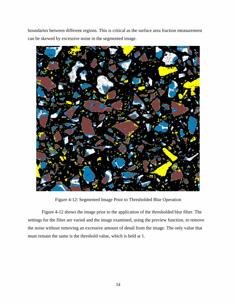
54
boundaries between different regions. This is critical as the surface area fraction measurement
can be skewed by excessive noise in the segmented image.
Figure 4-12: Segmented Image Prior to Thresholded Blur Operation
Figure 4-12 shows the image prior to the application of the thresholded blur filter. The
settings for the filter are varied and the image examined, using the preview function, to remove
the noise without removing an excessive amount of detail from the image. The only value that
must remain the same is the threshold value, which is held at 1.
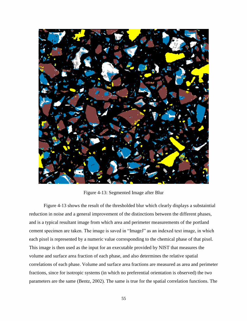
55
Figure 4-13: Segmented Image after Blur
Figure 4-13 shows the result of the thresholded blur which clearly displays a substaintial
reduction in noise and a general improvement of the distinctions between the different phases,
and is a typical resultant image from which area and perimeter measurements of the portland
cement specimen are taken. The image is saved in “ImageJ” as an indexed text image, in which
each pixel is represented by a numeric value corresponding to the chemical phase of that pixel.
This image is then used as the input for an executable provided by NIST that measures the
volume and surface area fraction of each phase, and also determines the relative spatial
correlations of each phase. Volume and surface area fractions are measured as area and perimeter
fractions, since for isotropic systems (in which no preferential orientation is observed) the two
parameters are the same (Bentz, 2002). The same is true for the spatial correlation functions. The
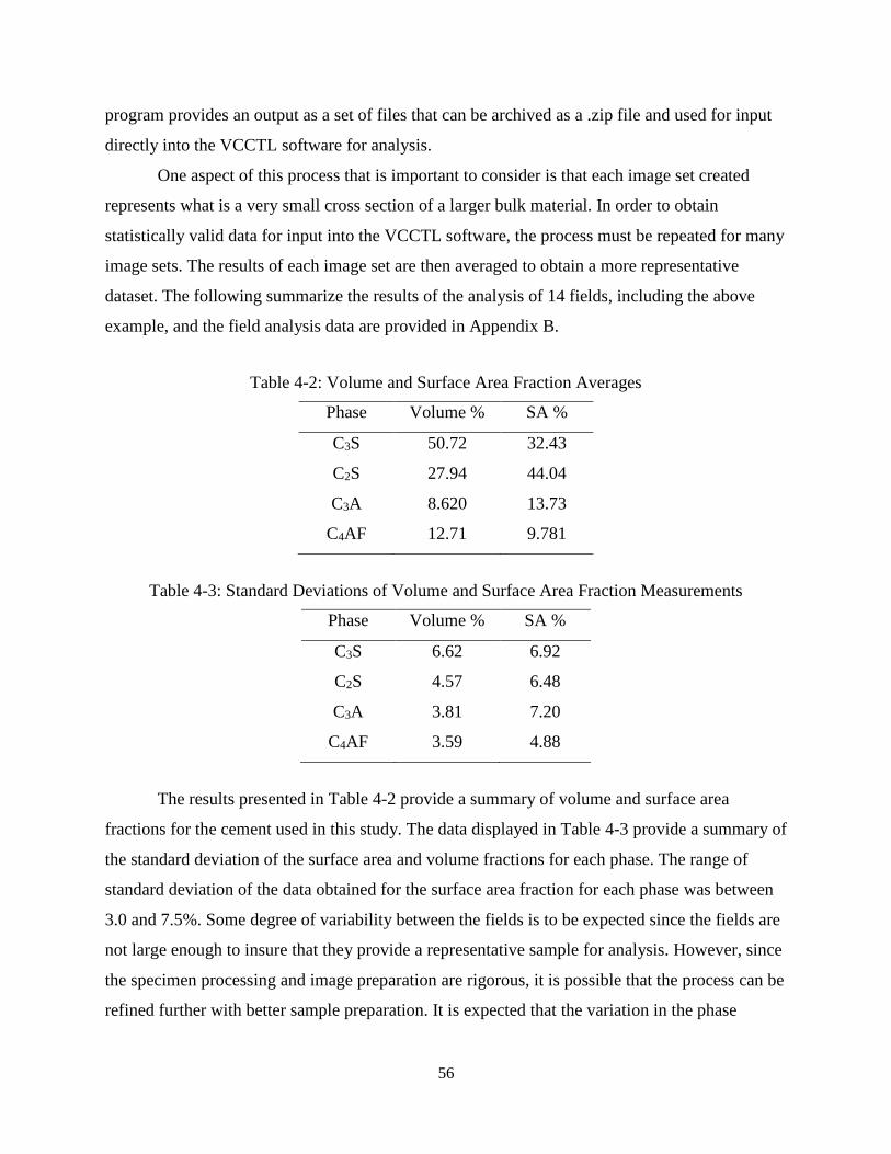
56
program provides an output as a set of files that can be archived as a .zip file and used for input
directly into the VCCTL software for analysis.
One aspect of this process that is important to consider is that each image set created
represents what is a very small cross section of a larger bulk material. In order to obtain
statistically valid data for input into the VCCTL software, the process must be repeated for many
image sets. The results of each image set are then averaged to obtain a more representative
dataset. The following summarize the results of the analysis of 14 fields, including the above
example, and the field analysis data are provided in Appendix B.
Table 4-2: Volume and Surface Area Fraction Averages
Phase Volume % SA %
C3S 50.72 32.43
C2S 27.94 44.04
C3A 8.620 13.73
C4AF 12.71 9.781
Table 4-3: Standard Deviations of Volume and Surface Area Fraction Measurements
Phase Volume % SA %
C3S 6.62 6.92
C2S 4.57 6.48
C3A 3.81 7.20
C4AF 3.59 4.88
The results presented in Table 4-2 provide a summary of volume and surface area
fractions for the cement used in this study. The data displayed in Table 4-3 provide a summary of
the standard deviation of the surface area and volume fractions for each phase. The range of
standard deviation of the data obtained for the surface area fraction for each phase was between
3.0 and 7.5%. Some degree of variability between the fields is to be expected since the fields are
not large enough to insure that they provide a representative sample for analysis. However, since
the specimen processing and image preparation are rigorous, it is possible that the process can be
refined further with better sample preparation. It is expected that the variation in the phase

57
acquisition from image analysis of SEM EDS data can be reduced by acquiring a better final
polish of the samples analyzed.
This phase composition data can also be compared to that obtained from x-ray powder
diffraction data using Rietveld analysis. The refinement of this process is an ongoing effort, and
as they are further refined, the simulations should more closely represent the actual concretes
being simulated.
Automated Cement Characterization
Figure 4-14: Fields Analyzed by UF and RJ Lee Group Inc.
The process of acquiring fields and processing them to create a segmented image is very
labor intensive, has a fairly steep learning curve, and multiple fields must be collected to have
statistically valid data for the sample. Work was performed in cooperation with RJ Lee Group
Inc. to automate this process, with the purpose of reducing the time and operator skill required to
obtain proper cement images.
A preliminary comparison study was conducted to investigate the potential for automated
SEM field acquisition to reduce time and labor requirements for the process. The first part of this
study involved the manual acquisition of 15 fields (BSE and EDS maps) of a polished cement
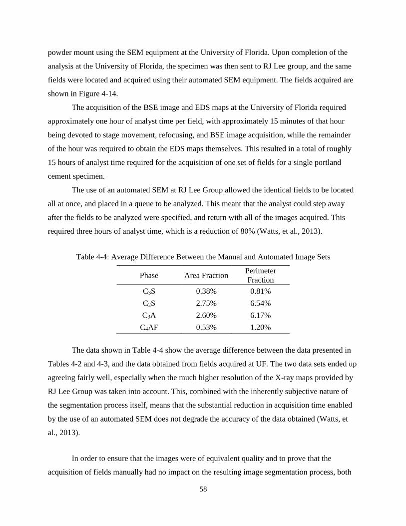
58
powder mount using the SEM equipment at the University of Florida. Upon completion of the
analysis at the University of Florida, the specimen was then sent to RJ Lee group, and the same
fields were located and acquired using their automated SEM equipment. The fields acquired are
shown in Figure 4-14.
The acquisition of the BSE image and EDS maps at the University of Florida required
approximately one hour of analyst time per field, with approximately 15 minutes of that hour
being devoted to stage movement, refocusing, and BSE image acquisition, while the remainder
of the hour was required to obtain the EDS maps themselves. This resulted in a total of roughly
15 hours of analyst time required for the acquisition of one set of fields for a single portland
cement specimen.
The use of an automated SEM at RJ Lee Group allowed the identical fields to be located
all at once, and placed in a queue to be analyzed. This meant that the analyst could step away
after the fields to be analyzed were specified, and return with all of the images acquired. This
required three hours of analyst time, which is a reduction of 80% (Watts, et al., 2013).
Table 4-4: Average Difference Between the Manual and Automated Image Sets
Phase Area Fraction Perimeter
Fraction
C3S 0.38% 0.81%
C2S 2.75% 6.54%
C3A 2.60% 6.17%
C4AF 0.53% 1.20%
The data shown in Table 4-4 show the average difference between the data presented in
Tables 4-2 and 4-3, and the data obtained from fields acquired at UF. The two data sets ended up
agreeing fairly well, especially when the much higher resolution of the X-ray maps provided by
RJ Lee Group was taken into account. This, combined with the inherently subjective nature of
the segmentation process itself, means that the substantial reduction in acquisition time enabled
by the use of an automated SEM does not degrade the accuracy of the data obtained (Watts, et
al., 2013).
In order to ensure that the images were of equivalent quality and to prove that the
acquisition of fields manually had no impact on the resulting image segmentation process, both
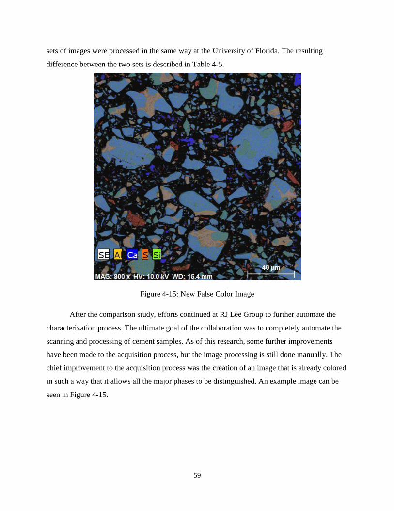
59
sets of images were processed in the same way at the University of Florida. The resulting
difference between the two sets is described in Table 4-5.
Figure 4-15: New False Color Image
After the comparison study, efforts continued at RJ Lee Group to further automate the
characterization process. The ultimate goal of the collaboration was to completely automate the
scanning and processing of cement samples. As of this research, some further improvements
have been made to the acquisition process, but the image processing is still done manually. The
chief improvement to the acquisition process was the creation of an image that is already colored
in such a way that it allows all the major phases to be distinguished. An example image can be
seen in Figure 4-15.

60
Figure 4-16: After Processing, Image Ready for Classification
This image was supplied directly from RJ Lee, and it eliminated the process of
combining the x-ray maps and backscatter electron images. Different colors were assigned to
different elements, as shown in the key at the lower left of Figure 4-15, and the resulting shades
indicate the relative mass percentages of the elements present. The best example of this can be
seen in the difference between alite and belite. Silicon was assigned to green, and calcium was
assigned to blue, and because belite (C2S) has a higher ratio of silicon to calcium, it showed up
as a greener shade of blue-green, while alite appeared bluer.
This image was cropped, levels were adjusted, and the thresholded blur filter described
earlier was applied to reduce noise. The resulting image, shown in Figure 4-16, was able to be
classified in Multispec immediately. Image analysis proceeded as usual after this image was
loaded into Multispec.
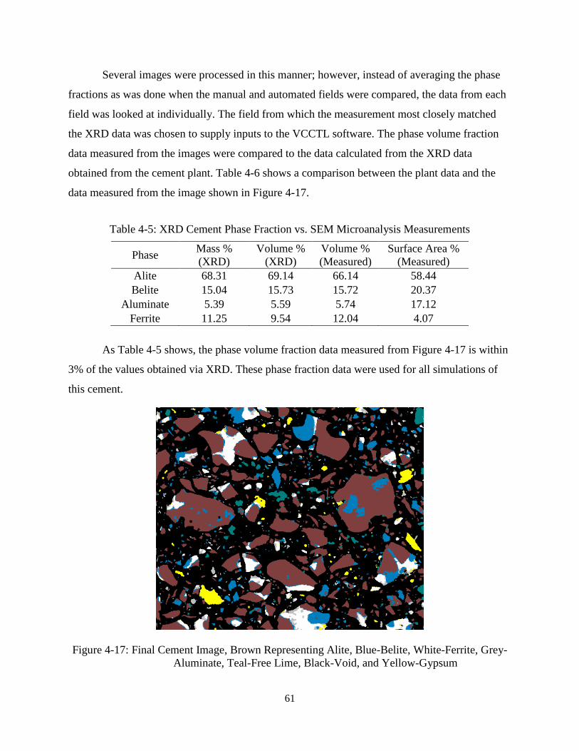
61
Several images were processed in this manner; however, instead of averaging the phase
fractions as was done when the manual and automated fields were compared, the data from each
field was looked at individually. The field from which the measurement most closely matched
the XRD data was chosen to supply inputs to the VCCTL software. The phase volume fraction
data measured from the images were compared to the data calculated from the XRD data
obtained from the cement plant. Table 4-6 shows a comparison between the plant data and the
data measured from the image shown in Figure 4-17.
Table 4-5: XRD Cement Phase Fraction vs. SEM Microanalysis Measurements
Phase Mass %
(XRD)
Volume %
(XRD)
Volume %
(Measured)
Surface Area %
(Measured)
Alite 68.31 69.14 66.14 58.44
Belite 15.04 15.73 15.72 20.37
Aluminate 5.39 5.59 5.74 17.12
Ferrite 11.25 9.54 12.04 4.07
As Table 4-5 shows, the phase volume fraction data measured from Figure 4-17 is within
3% of the values obtained via XRD. These phase fraction data were used for all simulations of
this cement.
Figure 4-17: Final Cement Image, Brown Representing Alite, Blue-Belite, White-Ferrite, Grey-
Aluminate, Teal-Free Lime, Black-Void, and Yellow-Gypsum

62
It was decided to utilize data from an individual field rather than the average of several
fields because the availability of the mass fraction data from XRD (obtained in earlier analyses)
revealed that the image analyses systematically overestimated the volume fractions of certain
phases, particularly alite and belite. Since the accuracy of phase characterization is the ultimate
goal for this technique, it was deemed acceptable to pick an individual field that matched the
XRD data closely because of the standardized and well established nature of the XRD test.
63
CHAPTER 5 VCCTL SOFTWARE OUTPUT DATA
Overview
The outputs provided by the VCCTL software can be divided in to two categories. There
are properties that are computed and measured continuously as part of the hydration simulation,
and are referred to as continuous measurements by the software. There are outputs that result
from additional simulations calculated using a snapshot of the hydrated microstructure as an
input, which are referred to as periodic measurements by the model because they can only be
performed on static microstructures that have been saved at user specified intervals. The
following list provides the potential outputs from the software:
Cement and hydration product phase volume fractions;
Solution concentration of sodium, potassium, calcium, sulfate;
Solution activity of sodium, potassium, calcium, sulfate;
Total porosity;
Fraction porosity connected in the x, y, and z directions;
Average fraction porosity connected;
Fraction solids connected in the x, y, and z direction;
Average fraction solids connected;
Solution pH;
Solution conductivity;
Non-evaporable water content (ignited and unignited);
Gel/space ratio;
Binder temperature;
Heat release;
Degree of hydration;
Cycles run;
Elastic modulus of the paste;
Elastic modulus of the concrete; and
Strength of the concrete.
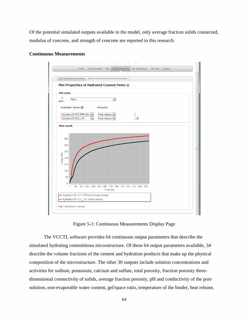
64
Of the potential simulated outputs available in the model, only average fraction solids connected,
modulus of concrete, and strength of concrete are reported in this research.
Continuous Measurements
Figure 5-1: Continuous Measurements Display Page
The VCCTL software provides 64 continuous output parameters that describe the
simulated hydrating cementitious microstructure. Of these 64 output parameters available, 34
describe the volume fractions of the cement and hydration products that make up the physical
composition of the microstructure. The other 30 outputs include solution concentrations and
activities for sodium, potassium, calcium and sulfate, total porosity, fraction porosity three-
dimensional connectivity of solids, average fraction porosity, pH and conductivity of the pore
solution, non-evaporable water content, gel/space ratio, temperature of the binder, heat release,
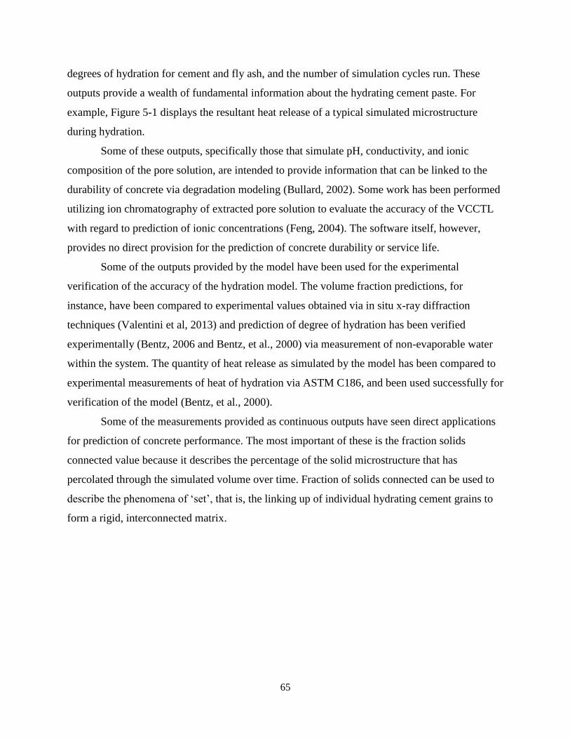
65
degrees of hydration for cement and fly ash, and the number of simulation cycles run. These
outputs provide a wealth of fundamental information about the hydrating cement paste. For
example, Figure 5-1 displays the resultant heat release of a typical simulated microstructure
during hydration.
Some of these outputs, specifically those that simulate pH, conductivity, and ionic
composition of the pore solution, are intended to provide information that can be linked to the
durability of concrete via degradation modeling (Bullard, 2002). Some work has been performed
utilizing ion chromatography of extracted pore solution to evaluate the accuracy of the VCCTL
with regard to prediction of ionic concentrations (Feng, 2004). The software itself, however,
provides no direct provision for the prediction of concrete durability or service life.
Some of the outputs provided by the model have been used for the experimental
verification of the accuracy of the hydration model. The volume fraction predictions, for
instance, have been compared to experimental values obtained via in situ x-ray diffraction
techniques (Valentini et al, 2013) and prediction of degree of hydration has been verified
experimentally (Bentz, 2006 and Bentz, et al., 2000) via measurement of non-evaporable water
within the system. The quantity of heat release as simulated by the model has been compared to
experimental measurements of heat of hydration via ASTM C186, and been used successfully for
verification of the model (Bentz, et al., 2000).
Some of the measurements provided as continuous outputs have seen direct applications
for prediction of concrete performance. The most important of these is the fraction solids
connected value because it describes the percentage of the solid microstructure that has
percolated through the simulated volume over time. Fraction of solids connected can be used to
describe the phenomena of ‘set’, that is, the linking up of individual hydrating cement grains to
form a rigid, interconnected matrix.
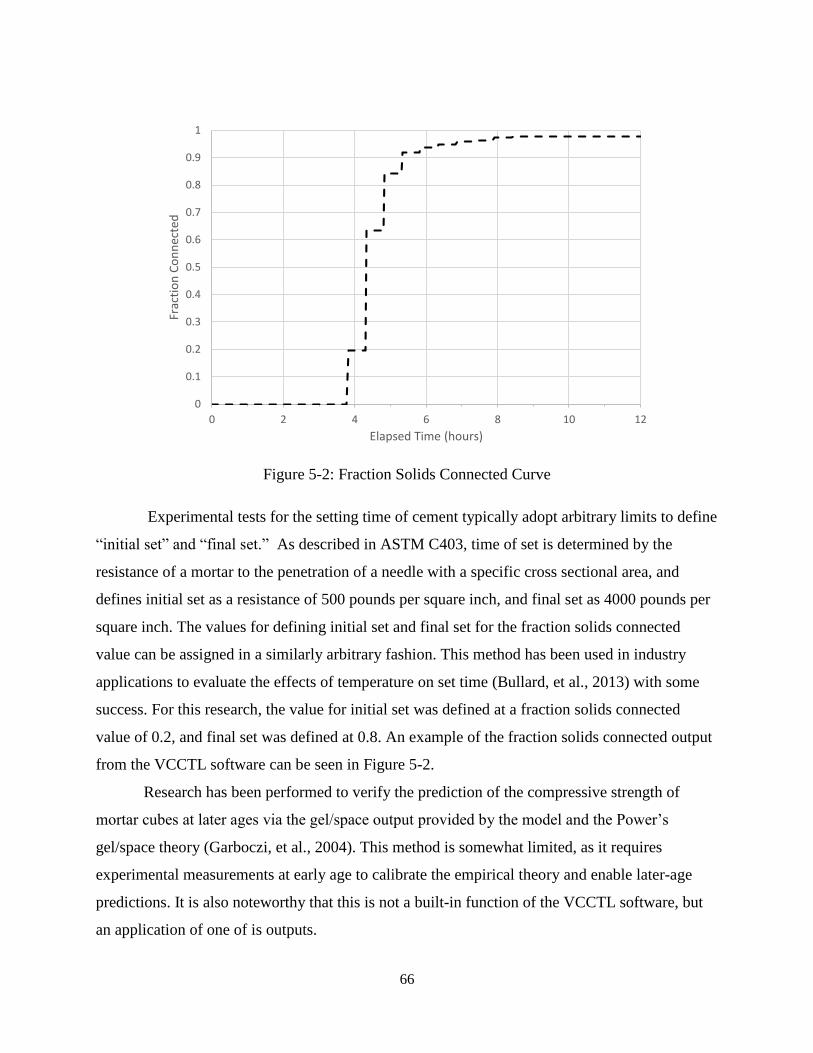
66
Figure 5-2: Fraction Solids Connected Curve
Experimental tests for the setting time of cement typically adopt arbitrary limits to define
“initial set” and “final set.” As described in ASTM C403, time of set is determined by the
resistance of a mortar to the penetration of a needle with a specific cross sectional area, and
defines initial set as a resistance of 500 pounds per square inch, and final set as 4000 pounds per
square inch. The values for defining initial set and final set for the fraction solids connected
value can be assigned in a similarly arbitrary fashion. This method has been used in industry
applications to evaluate the effects of temperature on set time (Bullard, et al., 2013) with some
success. For this research, the value for initial set was defined at a fraction solids connected
value of 0.2, and final set was defined at 0.8. An example of the fraction solids connected output
from the VCCTL software can be seen in Figure 5-2.
Research has been performed to verify the prediction of the compressive strength of
mortar cubes at later ages via the gel/space output provided by the model and the Power’s
gel/space theory (Garboczi, et al., 2004). This method is somewhat limited, as it requires
experimental measurements at early age to calibrate the empirical theory and enable later-age
predictions. It is also noteworthy that this is not a built-in function of the VCCTL software, but
an application of one of is outputs.
0
0.1
0.2
0.3
0.4
0.5
0.6
0.7
0.8
0.9
1
0 2 4 6 8 10 12
Frac
tio
n C
on
nec
ted
Elapsed Time (hours)

67
Periodic Measurements
Figure 5-3: Periodic Measurement Display Page
The second category of measurements are those obtained from calculations run on
hydrated microstructures of various ages. It is from these outputs that elastic modulus and
strength properties are obtained. The measurements screen for periodic outputs is shown in
Figure 5-3.
Elastic Modulus
The VCCTL software computes the elastic moduli of hydrated cement paste, mortar or
concrete and is first computed from the hydrated microstructure using a finite element model.
68
The resulting modulus of the paste is then used as an input for another, slightly different finite
element calculation which incorporates the modulus of the concrete, based on the computed
paste modulus as well as the input bulk and shear moduli for the aggregates used. A summary of
the methods by which these computations are executed is summarized in the following sections.
Hydrated Cement Microstructure Modulus
The elastic modulus of hydrated cement paste is computed using an effective medium
theory (EMT) for three-dimensional spherical particles (Garboczi & Day 1995). This theory
calculates the bulk and shear moduli of the composite paste using known values of the bulk and
shear moduli and volume fractions of each specific phase present in the paste. The equations
used to calculate the effective shear and bulk moduli of the paste are as follows:
1
𝐺=
𝑐1
𝐺+𝛽(𝐺1−𝐺)+
𝑐2
𝐺+𝛽(𝐺2−𝐺)… +
𝑐𝑛
𝐺+𝛽(𝐺𝑛−𝐺) (5-1)
1
𝐾=
𝑐1
𝐾+𝛼(𝐾1−𝐾)+
𝑐2
𝐾+𝛼(𝐾2−𝐾)… +
𝑐𝑛
𝐾+𝛼(𝐾𝑛−𝐾) (5-2)
𝛽 =2(4−5𝜈)
15(1−𝜈) (5-3)
𝛼 =2(4−5𝜈)
15(1−𝜈) (5-4)
Where:
G and Gn, K and Kn are the shear and bulk moduli (GPa) of the composite and nth phase;
𝜈 is the Poisson’s ratio of the composite;
cn is the volume fraction of the nth phase; and 𝛼 and 𝛽 are dimensionless constants.
An algorithm which utilizes equations (5-1) - (5-4) simulates the composite elastic
modulus of the three-dimensional microstructure by treating the digital image as a mesh of linear
finite elements, where each voxel is an element. Individual phase properties are assigned to each
voxel, and composite properties are computed by applying a strain and computing the
appropriate energy averages (Garboczi & Day, 1995).

69
Concrete and Mortar Modulus
The resulting modulus of the paste is then used to calculate the modulus of the concrete.
This calculation uses a more complex differential EMT, which models the concrete as a matrix
with spherical inclusions. The inclusions are composite elements composed of individual
aggregate particles that are surrounded by thin shells of altered matrix material (representing the
interfacial transition zone). The aggregates and surrounding shells are mapped as a single particle
with a diameter equal to that of the outer shell. The effective or composite moduli are calculated
from the moduli of the particle and shell. The equations to perform this mapping are quite
lengthy, and detailed in Appendix A.
The new effective particles are larger than the original aggregate particles, and thus the
original particle volume fractions must be normalized to account for the change in diameter. The
equations used to perform this normalization are as follows:
𝛼𝑗 =𝑎𝑗
3
𝑏𝑗3 (5-5)
𝑐′ = 𝑐 ∑ 𝑓𝑗𝑀𝑗=1 𝛼𝑗 (5-6)
𝑓′𝑗 =𝑓𝑗𝛼𝑗
∑ 𝑓𝑗𝛼𝑗𝑀𝑗=1
(5-7)
Where:
𝑐 = original volume fraction;
𝑐′= normalized volume fraction;
𝑓𝑗 = original partial volume fraction of the jth type of particle lying in a certain diameter
range;
𝑓′𝑗= normalized partial volume fractions of the jth type of particle lying in a certain
diameter range;
𝑏𝑗= the diameter (in microns) of the original particle; and
𝛼𝑗= the diameter of the jth type new effective particle.
The resulting bulk and shear moduli are solved for numerically using a set of differential
equations detailed in Appendix A. This numerical method was verified using the same method
by which the cement paste modulus is calculated, that is a three-dimensional digital image was
built with the aggregates and their surrounding zones of altered matrix material, and the effective
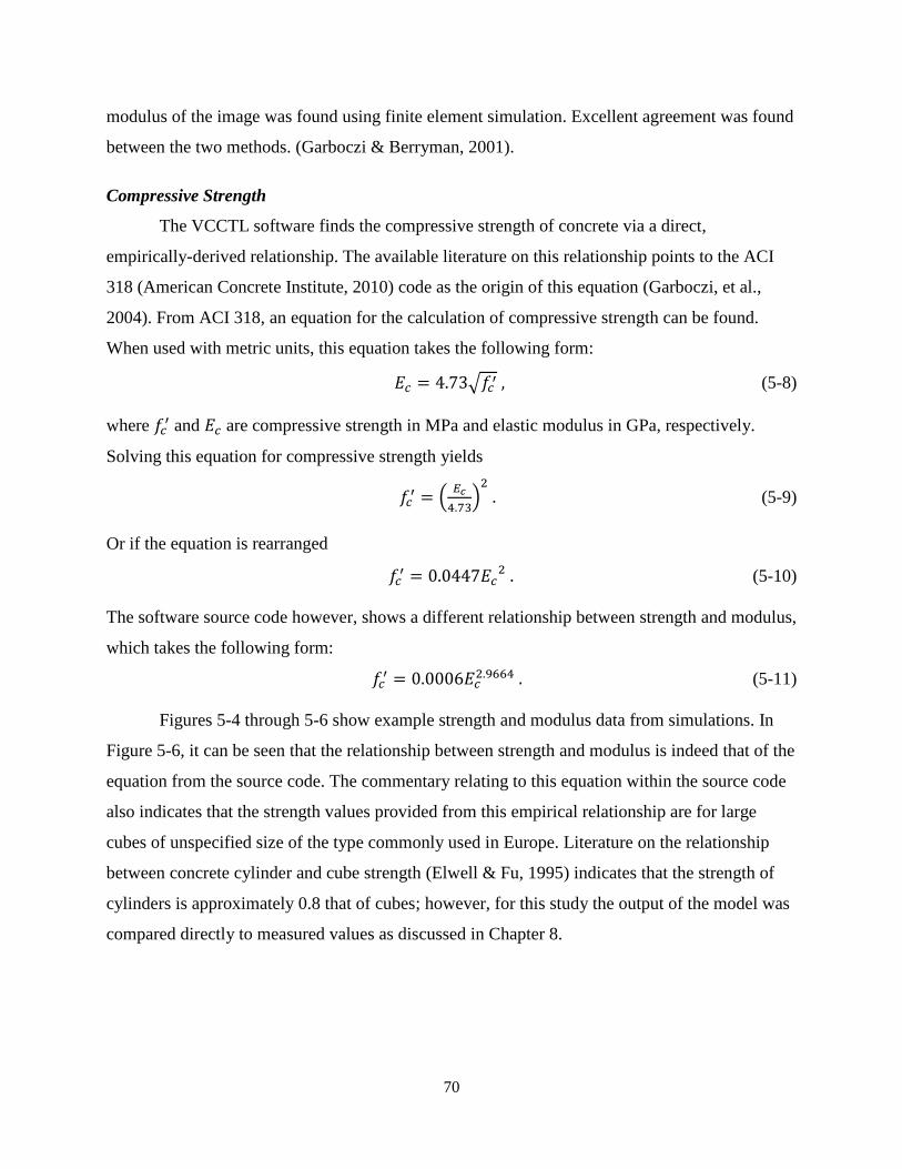
70
modulus of the image was found using finite element simulation. Excellent agreement was found
between the two methods. (Garboczi & Berryman, 2001).
Compressive Strength
The VCCTL software finds the compressive strength of concrete via a direct,
empirically-derived relationship. The available literature on this relationship points to the ACI
318 (American Concrete Institute, 2010) code as the origin of this equation (Garboczi, et al.,
2004). From ACI 318, an equation for the calculation of compressive strength can be found.
When used with metric units, this equation takes the following form:
𝐸𝑐 = 4.73√𝑓𝑐′ , (5-8)
where 𝑓𝑐′ and 𝐸𝑐 are compressive strength in MPa and elastic modulus in GPa, respectively.
Solving this equation for compressive strength yields
𝑓𝑐′ = (
𝐸𝑐
4.73)
2
. (5-9)
Or if the equation is rearranged
𝑓𝑐′ = 0.0447𝐸𝑐
2 . (5-10)
The software source code however, shows a different relationship between strength and modulus,
which takes the following form:
𝑓𝑐′ = 0.0006𝐸𝑐
2.9664 . (5-11)
Figures 5-4 through 5-6 show example strength and modulus data from simulations. In
Figure 5-6, it can be seen that the relationship between strength and modulus is indeed that of the
equation from the source code. The commentary relating to this equation within the source code
also indicates that the strength values provided from this empirical relationship are for large
cubes of unspecified size of the type commonly used in Europe. Literature on the relationship
between concrete cylinder and cube strength (Elwell & Fu, 1995) indicates that the strength of
cylinders is approximately 0.8 that of cubes; however, for this study the output of the model was
compared directly to measured values as discussed in Chapter 8.
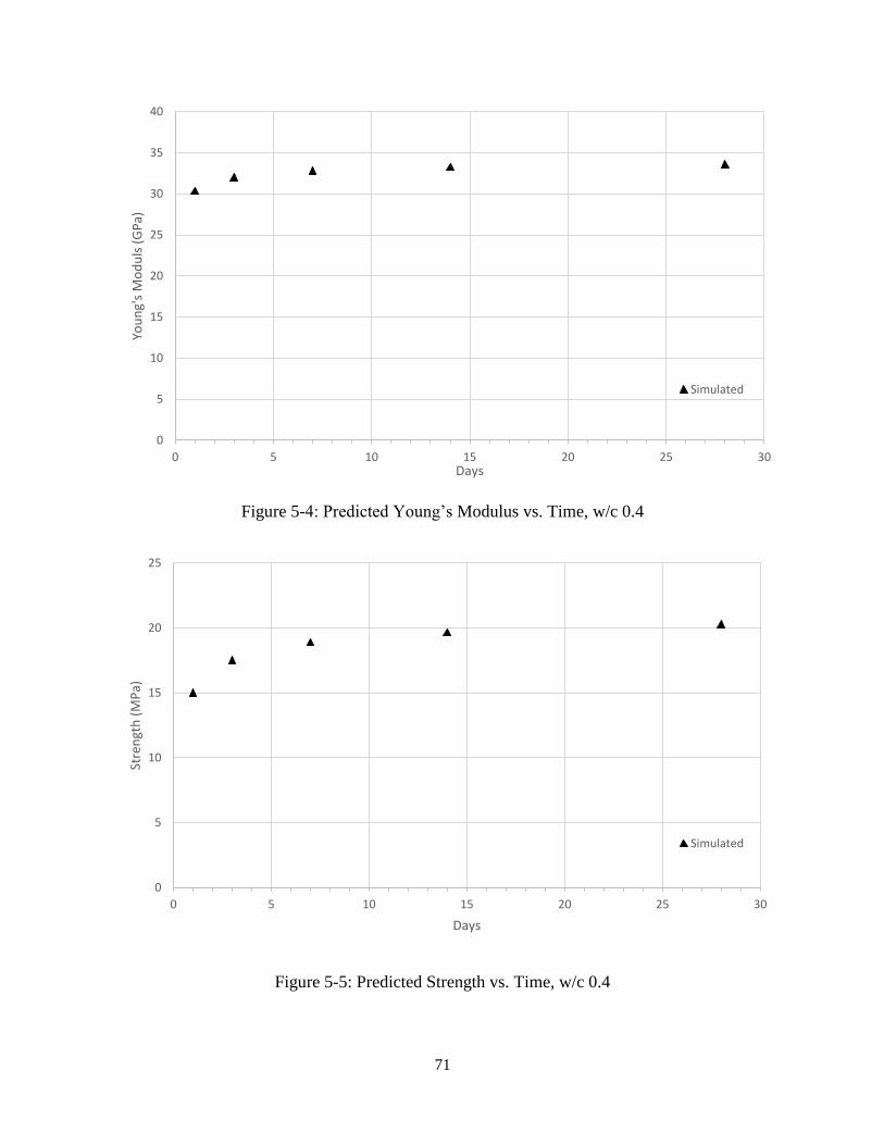
71
Figure 5-4: Predicted Young’s Modulus vs. Time, w/c 0.4
Figure 5-5: Predicted Strength vs. Time, w/c 0.4
0
5
10
15
20
25
30
35
40
0 5 10 15 20 25 30
You
ng'
s M
od
uls
(G
Pa)
Days
Simulated
0
5
10
15
20
25
0 5 10 15 20 25 30
Stre
ngt
h (
MP
a)
Days
Simulated
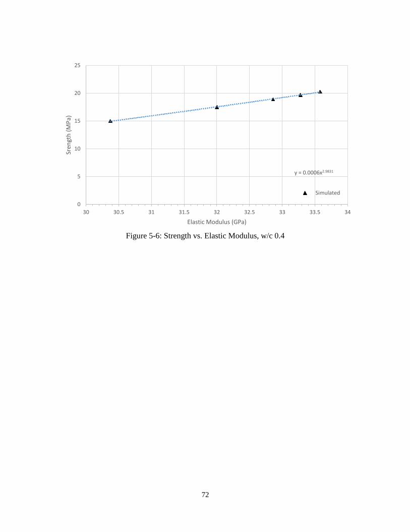
72
Figure 5-6: Strength vs. Elastic Modulus, w/c 0.4
y = 0.0006x2.9831
0
5
10
15
20
25
30 30.5 31 31.5 32 32.5 33 33.5 34
Sren
gth
(M
Pa)
Elastic Modulus (GPa)
Simulated
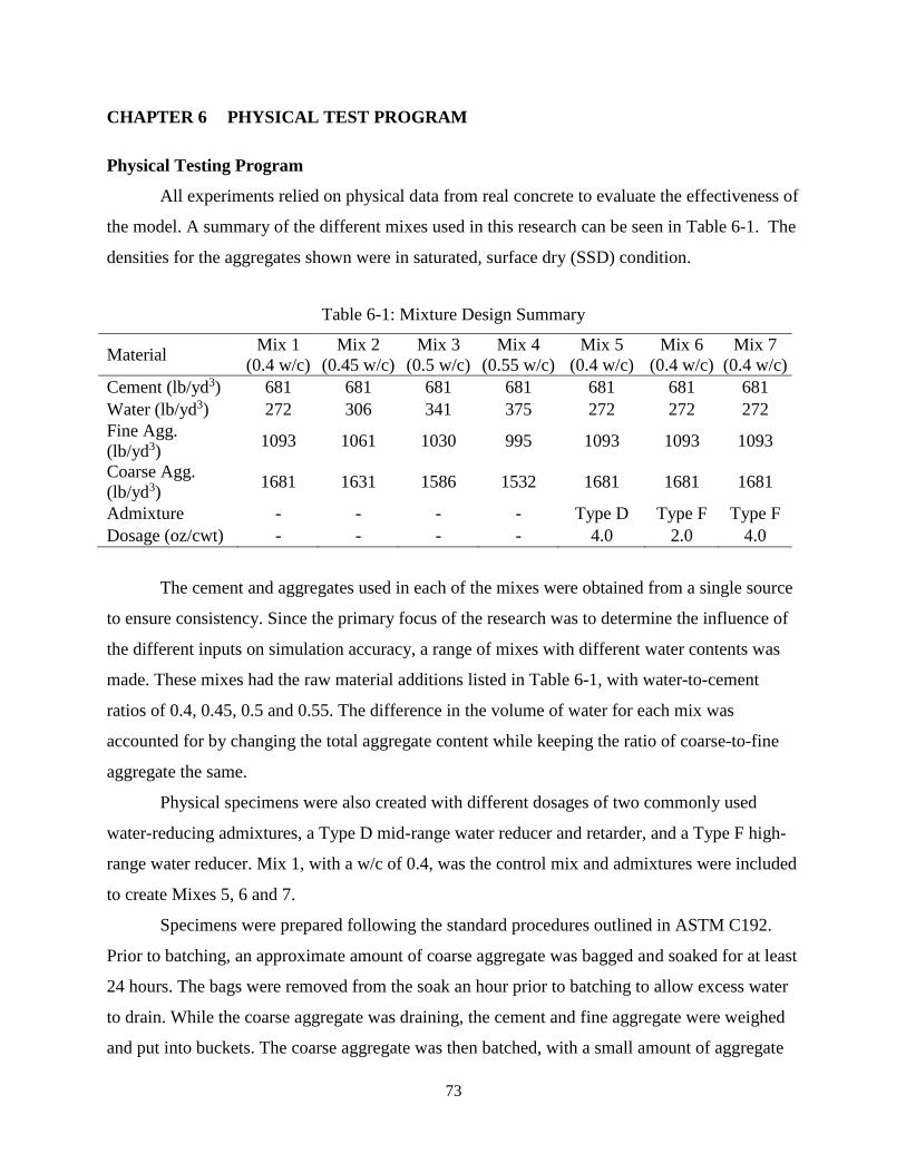
73
CHAPTER 6 PHYSICAL TEST PROGRAM
Physical Testing Program
All experiments relied on physical data from real concrete to evaluate the effectiveness of
the model. A summary of the different mixes used in this research can be seen in Table 6-1. The
densities for the aggregates shown were in saturated, surface dry (SSD) condition.
Table 6-1: Mixture Design Summary
Material Mix 1
(0.4 w/c)
Mix 2
(0.45 w/c)
Mix 3
(0.5 w/c)
Mix 4
(0.55 w/c)
Mix 5
(0.4 w/c)
Mix 6
(0.4 w/c)
Mix 7
(0.4 w/c)
Cement (lb/yd3) 681 681 681 681 681 681 681
Water (lb/yd3) 272 306 341 375 272 272 272
Fine Agg.
(lb/yd3) 1093 1061 1030 995 1093 1093 1093
Coarse Agg.
(lb/yd3) 1681 1631 1586 1532 1681 1681 1681
Admixture - - - - Type D Type F Type F
Dosage (oz/cwt) - - - - 4.0 2.0 4.0
The cement and aggregates used in each of the mixes were obtained from a single source
to ensure consistency. Since the primary focus of the research was to determine the influence of
the different inputs on simulation accuracy, a range of mixes with different water contents was
made. These mixes had the raw material additions listed in Table 6-1, with water-to-cement
ratios of 0.4, 0.45, 0.5 and 0.55. The difference in the volume of water for each mix was
accounted for by changing the total aggregate content while keeping the ratio of coarse-to-fine
aggregate the same.
Physical specimens were also created with different dosages of two commonly used
water-reducing admixtures, a Type D mid-range water reducer and retarder, and a Type F high-
range water reducer. Mix 1, with a w/c of 0.4, was the control mix and admixtures were included
to create Mixes 5, 6 and 7.
Specimens were prepared following the standard procedures outlined in ASTM C192.
Prior to batching, an approximate amount of coarse aggregate was bagged and soaked for at least
24 hours. The bags were removed from the soak an hour prior to batching to allow excess water
to drain. While the coarse aggregate was draining, the cement and fine aggregate were weighed
and put into buckets. The coarse aggregate was then batched, with a small amount of aggregate

74
set aside from each bag for determination of moisture content. The aggregate set aside was
weighed wet, then put into the oven overnight to remove all moisture following the procedures
outlined in ASTM C566. The following day the water content and coarse aggregate contents
were adjusted based on the difference between the measured moisture content and the SSD
moisture content.
A small initial concrete batch, approximately 10% the size of the primary batch, was
prepared; this served to coat the inside of the mixer with mortar, and prevent any mortar loss of
the primary mix. Coarse and fine aggregates along with approximately half the water were then
added to the mixer and mixed until evenly distributed. The cement and remaining water were
added and mixed for three minutes. The concrete was then allowed to rest for approximately
three minutes. Following this step the admixture (if any) was added and the concrete was mixed
for another three minutes.
Each of the concrete batches were tested for unit weight (ASTM C138), temperature
(ASTM C1064), and air content (ASTM C138) in accordance with the ASTM standard method
for each respective test. Mixes containing admixtures also had a portion of their mortar sieved
out and placed into molds for the time of set test (ASTM C403). The results for the air content,
unit weight, temperature, and slump tests are shown in Table 6-2. Mixes three and four were too
fluid for the slump test to be performed to ASTM standards.
Table 6-2: Summary of Test Results for Fresh Concrete
Material Mix 1 Mix 2 Mix 3 Mix 4 Mix 5 Mix 6 Mix 7
Temperature (°F) 75 72 74 75 76 74 74
Air Content (%) 2.5 2.25 0.3 0.0 3.0 3.0 3.75
Unit Weight
(lb/yd3) 143.4 142.2 139.1 137.7 141.3 140.5 142.16

75
Figure 6-1: Preparation of Cylinders
Figure 6-2: Elastic Modulus and Compressive Strength Testing
Each batch of thirty-eight 4” by 8” test cylinders were used for the creation of specimens
for the testing of compressive strength and modulus in accordance with ASTM C192. Cylinders

76
were filled in two lifts, with a vibratory table used for 15 seconds between each lift to
consolidate the concrete as depicted in Figure 6-1. Cylinders were then capped and cured for 24
hours prior to stripping the molds and the first strength and modulus tests. The time of set test
was run in accordance with ASTM C403, penetration testing began at two hours, after which
penetration resistance measurements were taken at regular intervals. The apparatus for the
penetration resistance test is shown in Figure 6-3.
Hardened cylinders were ground flat on both ends and tested for compressive strength
and elastic modulus in accordance with ASTM C39 and ASTM C 469, respectively. Figure 6-2
provides an illustration of these tests. Strength and modulus values were obtained at 1, 3, 7, 14,
and 28 days in order to provide a wide range of time scales for the evaluation of the accuracy of
the VCCTL software.
Figure 6-3: Time of Set Test Apparatus
Isothermal Calorimetry
Isothermal calorimetry data were collected for each of the mixes that contained
admixtures, as well as the control mix with the w/c of 0.4. For each cement, water, and
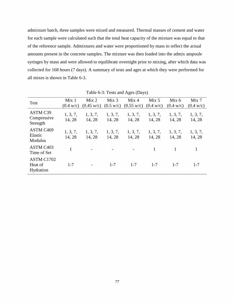
77
admixture batch, three samples were mixed and measured. Thermal masses of cement and water
for each sample were calculated such that the total heat capacity of the mixture was equal to that
of the reference sample. Admixtures and water were proportioned by mass to reflect the actual
amounts present in the concrete samples. The mixture was then loaded into the admix ampoule
syringes by mass and were allowed to equilibrate overnight prior to mixing, after which data was
collected for 168 hours (7 days). A summary of tests and ages at which they were performed for
all mixes is shown in Table 6-3.
Table 6-3: Tests and Ages (Days)
Test Mix 1
(0.4 w/c)
Mix 2
(0.45 w/c)
Mix 3
(0.5 w/c)
Mix 4
(0.55 w/c)
Mix 5
(0.4 w/c)
Mix 6
(0.4 w/c)
Mix 7
(0.4 w/c)
ASTM C39
Compressive
Strength
1, 3, 7,
14, 28
1, 3, 7,
14, 28
1, 3, 7,
14, 28
1, 3, 7,
14, 28
1, 3, 7,
14, 28
1, 3, 7,
14, 28
1, 3, 7,
14, 28
ASTM C469
Elastic
Modulus
1, 3, 7,
14, 28
1, 3, 7,
14, 28
1, 3, 7,
14, 28
1, 3, 7,
14, 28
1, 3, 7,
14, 28
1, 3, 7,
14, 28
1, 3, 7,
14, 28
ASTM C403
Time of Set 1 - - - 1 1 1
ASTM C1702
Heat of
Hydration
1-7 - 1-7 1-7 1-7 1-7 1-7
78
CHAPTER 7 COMPARISON OF PHYSICAL TEST DATA TO MODEL OUTPUTS
Experimental Design
The primary objective of the experiments conducted for this research was to validate the
accuracy of the VCCTL software with regard to the simulation of the structural properties of
concrete (as opposed to mortar or grout), and assess its potential value as a tool for the
development of new concrete mixture designs. The vast majority of concrete mixes made today
contain both supplementary cementitious materials (SCMs), such as fly ash and silica fume, and
practically all mixes contain some type of chemical admixture. While mixes containing these
materials can be simulated by the software, the characterization of these materials requires the
development and refinement of procedures at least as complex as those for portland cement. The
scope of this project precluded the use of SCMs for the validation study, however a method by
which certain effects of some admixtures may be simulated was developed and investigated.
Currently, the VCCTL software does not possess the capability to properly model
concrete mixtures which incorporate supplementary cementitious materials; therefore, the
concrete mixture designs considered for the validation study contained portland cement as the
only cementitious component. With this restriction imposed, the decision to test the accuracy of
the simulations at a range of water-to-cement ratios was made. Water-to-cement ratio is widely
known (Mindess & Young, 1981) to be the most important variable that affects the strength and
elastic modulus of concrete. Concrete mixtures incorporating water-to-cement (w/c) ratios of 0.4,
0.45, 0.5, and 0.55 were selected, with the lower bound of 0.4 being the limit of feasible mixing
without any water-reducing admixture, and the upper limit of 0.55 being above the designed
water content of most mixes used in industry applications (Florida Department of Transportation,
2014). The experimental results for concrete mixtures created in the laboratory were compared
directly to the compressive strength and compressive modulus elasticity data predicted by the
software.
It was determined that investigating the influence of each of the different material inputs
accepted by the VCCTL software would be important for evaluating its usefulness as a concrete
mix design development tool. A control mix with a water-to-cement ratio of 0.4 was modeled
first using all available input data, then several simulations were performed on the same mixture
with a different non-essential input removed in each simulation. Because compressive strength is
calculated by the software from the modulus, based on a fixed empirical relationship, it was not
79
considered when comparing the influence of different input data. For the removal of inputs
which influence the hydration simulation, changes to the fraction solids connected curve were
also investigated.
Experiments were conducted to investigate the accuracy of simulation of some concrete
mixtures containing water-reducing admixtures which can increase the set time of fresh concrete
as discussed in Chapter 3. The effect can be measured in fresh concrete using the time of set test,
and can also be quantified using isothermal calorimetry. Since the VCCTL software utilizes heat
of hydration data to calibrate the time scale of a simulation, it was decided to investigate the
difference in set time obtained when isothermal calorimetry data were used from the hydration of
a cement with a water-reducing admixture. Additionally, it was postulated that the long-term
effects of the addition of a water-reducing admixture on strength and elastic modulus were
negligible when mixes of the same water-to-cement ratio were compared (Mamlouk &
Zaniewski, 2010). Given that this postulate holds true, this indirect method of accounting for
admixture behavior could prove to be a substantial enhancement to the practicality of the
software since the fraction solids connected value has been the primary output of the model used
to predict the changes in set time.
Simulation Procedures
Except for the mixes evaluating the sensitivity of the VCCTL software to the absence of
non-essential inputs as defined in Chapter 4, the mixes were simulated with the available,
measurable inputs. These inputs included cement phase volume and surface area fraction data
obtained via the SEM microanalysis method, the mass fraction data obtained from XRD analysis
for the different phases of gypsum, particle size distribution curves, isothermal calorimetry
curves, aggregate bulk and shear moduli, and aggregate shape data from the library of built-in
materials. Simulations were also performed with real particle shape data for the cement, which
was selected from the material library within the software database, based on its resemblance to
segmented imagery.
To simulate the effects of water-to-cement ratio, the only changes made to each mix were
the calorimetry curves, and the relative proportions of the mixes. Calorimetry data for the mix
with 0.45 water-to-cement ratio were unavailable; the calorimetry data used for the mix at 0.4
water-to-cement were used as a substitute. The aggregate mass fractions, cement content, and
water-to-cement ratio were modeled exactly as mixed. To gauge the sensitivity of the simulations

80
to the different non-essential inputs, several simulations were performed with selected inputs
absent or disabled. The simulations used to evaluate input sensitivity were based on a control
mix with a 0.4 w/c ratio. These included a mix with no calorimetry data, a mix with no real
particle shape data, a mix with no aggregate shape data, as well as a mix with a microstructure
50% larger (on a side) than normal. The influence of aggregate moduli was also investigated by
running three different Young’s moduli in three individual simulations.
For the investigation of set time simulation using measured isothermal calorimetry data,
four mixes were simulated with calorimetry data from three different admixture dosage
combinations. The effects of a Type D (mid-range) water reducer and retarder, at a dosage of 4
ounces per hundred pounds of cement (4 oz/cwt); Type F high-range water reducer, at dosages of
2 and 4 oz/cwt; and a control mixture, with no admixture present. Isothermal calorimetry curves
from each of these combinations were used in the simulations, and the mixes with admixtures
present had cement particle dispersion enabled. The physical test results of the four different w/c
are shown in Figures 7-1 and 7-2.
Results
Water-to-Cement Ratio
Figure 7-1: Compressive Strength vs. Time for Different w/c Ratios
0
10
20
30
40
50
60
0 5 10 15 20 25 30
Stre
ngt
h (
MP
a)
Time (Days)
0.4 w/c
0.45 w/c
0.5 w/c
0.55 w/c

81
Figure 7-2: Young’s Modulus vs. Time for Different w/c Ratios
Water-to-cement ratio (w/c) is one of the primary factors which affect compressive
strength, modulus of elasticity, and other properties of the microstructure, which affect the
general quality of concrete (Neville, 2011). The results presented in Figures 7-1 and 7-2 indicate
that the measured strength and elastic modulus of the mixes increased as the water-to-cement
ratio decreased.
Power and heat of hydration curves obtained via isothermal calorimetry for the different
w/c are shown in Figures 7-3 and 7-4. Figures 7-3 and 7-4 indicate that while there was very
little apparent difference between the maximum power outputs at the three different w/c, the
ultimate energy reached at 7 days (7-day heat of hydration) increased slightly with an increase in
w/c.
Figures 7-5 through 7-12 show comparisons of the strength and modulus results obtained
from physical testing to the simulated results calculated by the model. The error bars for the
physical test data represent plus or minus one standard deviation of the sample set average for
each measurement.
0
5
10
15
20
25
30
35
40
0 5 10 15 20 25 30
You
ng'
s M
od
uls
(G
Pa)
Time (Days)
0.4 w/c
0.45 w/c
0.5 w/c
0.55 w/c

82
Figure 7-3: Power vs. Time for Different w/c
Figure 7-4: Energy vs. Time for Different w/c
0.00
2.00
4.00
6.00
8.00
10.00
12.00
14.00
0 20 40 60 80 100 120 140 160
Po
wer
(m
w/g
)
Time (hours)
0.4 w/c
0.5 w/c
0.55 w/c
0.00
50.00
100.00
150.00
200.00
250.00
300.00
350.00
400.00
0 20 40 60 80 100 120 140 160
Ener
gy (
J/g)
Time (hours)
0.4 w/c
0.5 w/c
0.55 w/c

83
Figure 7-5: Young Modulus vs. Time, w/c of 0.4
Figure 7-6: Compressive Strength vs. Time, w/c of 0.4
0
5
10
15
20
25
30
35
40
0 5 10 15 20 25 30
You
ng'
s M
od
uls
(G
Pa)
Time (Days)
Measured
Simulated
0
10
20
30
40
50
60
0 5 10 15 20 25 30
Stre
ngt
h (
MP
a)
Time (Days)
Measured
Simulated

84
Figure 7-7: Young Modulus vs. Time, w/c of 0.45
Figure 7-8: Compressive Strength vs. Time, w/c of 0.45
0
5
10
15
20
25
30
35
40
0 5 10 15 20 25 30
You
ng'
s M
od
uls
(G
Pa)
Time (Days)
Measured
Simulated
0
10
20
30
40
50
60
0 5 10 15 20 25 30
Stre
ngt
h (
MP
a)
Time (Days)
Measured
Simulated

85
Figure 7-9: Young’s Modulus vs. Time, w/c of 0.5
Figure 7-10: Compressive Strength vs. Time, w/c of 0.5
0
5
10
15
20
25
30
35
0 5 10 15 20 25 30
You
ng'
s M
od
uls
(G
Pa)
Time (Days)
Measured
Simulated
0
5
10
15
20
25
30
35
40
0 5 10 15 20 25 30
Stre
ngt
h (
MP
a)
Time (Days)
Measured
Simulated
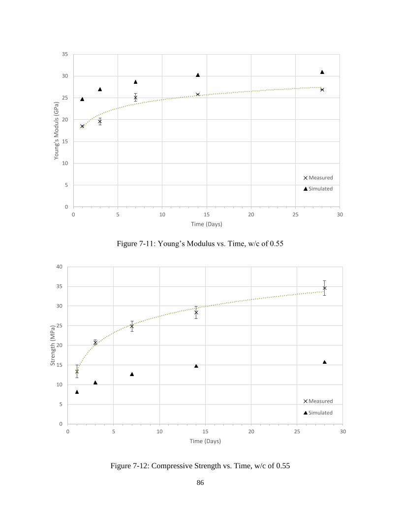
86
Figure 7-11: Young’s Modulus vs. Time, w/c of 0.55
Figure 7-12: Compressive Strength vs. Time, w/c of 0.55
0
5
10
15
20
25
30
35
0 5 10 15 20 25 30
You
ng'
s M
od
uls
(G
Pa)
Time (Days)
Measured
Simulated
0
5
10
15
20
25
30
35
40
0 5 10 15 20 25 30
Stre
ngt
h (
MP
a)
Time (Days)
Measured
Simulated

87
A comparison of Figures 7-1, 7-5, 7-7, and 7-9 indicates that the difference between the
simulated and measured values of Young’s modulus increased as w/c increased. The simulated
values overestimated early-age modulus, while predicting later-age modulus closely at lower
w/c. Simulated compressive strength was dramatically lower than measured compressive
strength at all w/c and ages.
Input Sensitivity Study
Figures 7-13, 7-14, and 7-15 present the effects of the removal of cement calorimetry
data, cement particle shape data, and aggregate shape data, respectively, relative to both the
simulated control sample with all available inputs and the measured values for the physical
control sample.
Figure 7-13: Young’s Modulus vs. Time, Removal of Calorimetry Data
0
5
10
15
20
25
30
35
40
0 5 10 15 20 25 30
You
ng'
s M
od
uls
(G
Pa)
Time (Days)
Measured
Simulated Control
No Calorimetry Data
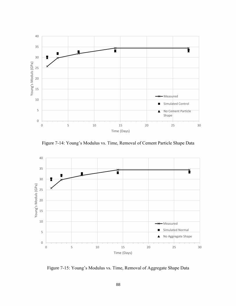
88
Figure 7-14: Young’s Modulus vs. Time, Removal of Cement Particle Shape Data
Figure 7-15: Young’s Modulus vs. Time, Removal of Aggregate Shape Data
0
5
10
15
20
25
30
35
40
0 5 10 15 20 25 30
You
ng'
s M
od
uls
(G
Pa)
Time (Days)
Measured
Simulated Control
No Cement ParticleShape
0
5
10
15
20
25
30
35
40
0 5 10 15 20 25 30
You
ng'
s M
od
uls
(G
Pa)
Time (Days)
Measured
Simulated Normal
No Aggregate Shape

89
The absence of aggregate shape data and cement particle shape data (Figures 7-14 and 7-
15) appeared to have very little influence on the simulated Young’s modulus, while absence of
calorimetry data (Figure 7-13) had a more dramatic effect on modulus. The simulation performed
without utilizing measured calorimetry data underestimated the Young’s modulus at early age,
which was in opposition to the simulation with the calorimetry data, which overestimated
modulus at early ages. At later ages, both simulations underestimated the modulus, with the no-
calorimetry-data simulation doing so to a slightly greater extent.
Figure 7-16: Young’s Modulus vs. Time, Larger Virtual Microstructure
The effect on a simulation performed with a microstructure 50% larger on a side is shown
by Figure 7-16. Similar to simulations performed without aggregate or cement particle shape, the
larger microstructure had very little influence on the simulated results. Of note is the increase in
the time required to run a simulation of a larger microstructure. The larger digital microstructure
was 50% longer in each direction, resulting in a volume 3.375 times larger than the original.
Thus the simulation of the larger digital microstructure took approximately 3.375 times longer.
0
5
10
15
20
25
30
35
40
0 5 10 15 20 25 30
You
ng'
s M
od
uls
(G
Pa)
Time (Days)
Measured
Simulated Normal
Simulated LargerMicrostructure
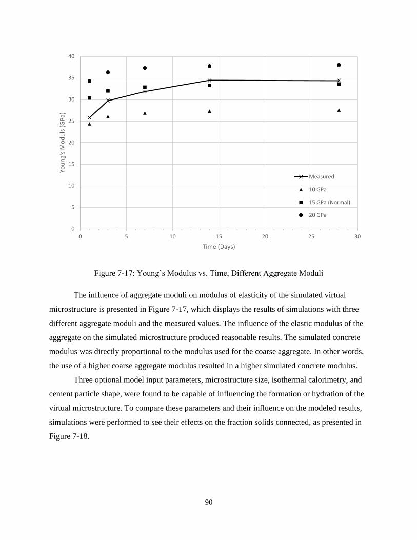
90
Figure 7-17: Young’s Modulus vs. Time, Different Aggregate Moduli
The influence of aggregate moduli on modulus of elasticity of the simulated virtual
microstructure is presented in Figure 7-17, which displays the results of simulations with three
different aggregate moduli and the measured values. The influence of the elastic modulus of the
aggregate on the simulated microstructure produced reasonable results. The simulated concrete
modulus was directly proportional to the modulus used for the coarse aggregate. In other words,
the use of a higher coarse aggregate modulus resulted in a higher simulated concrete modulus.
Three optional model input parameters, microstructure size, isothermal calorimetry, and
cement particle shape, were found to be capable of influencing the formation or hydration of the
virtual microstructure. To compare these parameters and their influence on the modeled results,
simulations were performed to see their effects on the fraction solids connected, as presented in
Figure 7-18.
0
5
10
15
20
25
30
35
40
0 5 10 15 20 25 30
You
ng'
s M
od
uls
(G
Pa)
Time (Days)
Measured
10 GPa
15 GPa (Normal)
20 GPa
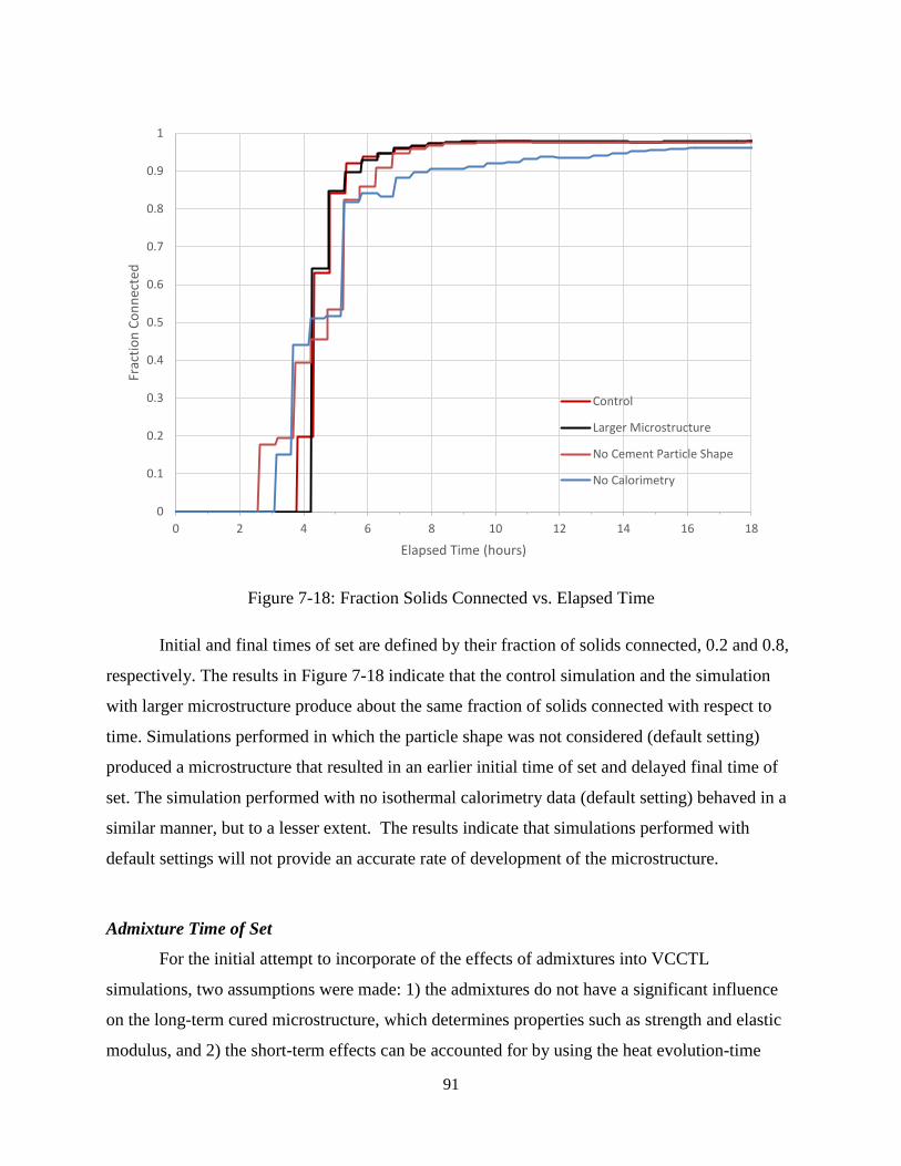
91
Figure 7-18: Fraction Solids Connected vs. Elapsed Time
Initial and final times of set are defined by their fraction of solids connected, 0.2 and 0.8,
respectively. The results in Figure 7-18 indicate that the control simulation and the simulation
with larger microstructure produce about the same fraction of solids connected with respect to
time. Simulations performed in which the particle shape was not considered (default setting)
produced a microstructure that resulted in an earlier initial time of set and delayed final time of
set. The simulation performed with no isothermal calorimetry data (default setting) behaved in a
similar manner, but to a lesser extent. The results indicate that simulations performed with
default settings will not provide an accurate rate of development of the microstructure.
Admixture Time of Set
For the initial attempt to incorporate of the effects of admixtures into VCCTL
simulations, two assumptions were made: 1) the admixtures do not have a significant influence
on the long-term cured microstructure, which determines properties such as strength and elastic
modulus, and 2) the short-term effects can be accounted for by using the heat evolution-time
0
0.1
0.2
0.3
0.4
0.5
0.6
0.7
0.8
0.9
1
0 2 4 6 8 10 12 14 16 18
Frac
tio
n C
on
nec
ted
Elapsed Time (hours)
Control
Larger Microstructure
No Cement Particle Shape
No Calorimetry

92
profile (from isothermal calorimetry) of the cementitious material plus admixtures instead of the
profile for just the cementitious material. The typical reason for incorporating chemical
admixtures into a concrete mixture is that the needed workability can be achieved with a reduced
w/c. A reduced w/c is desirable because it results in increased strength due to reduced residual
porosity.
The measured values for strength and elastic modulus for the mixes with different
admixture additions are shown in Figures 7-19 and 7-20 below. Error bars for the no-admixture
mix represent plus or minus one standard deviation of the sample data. Figures 7-19 and 7-20
indicate that the mix with 4 oz/cwt Type F admixture had a consistently higher strength and
modulus at all ages. The other mixes attained similar strength to the control mix. It should be
noted that even though the w/c was held constant at 0.4, the strength still significantly improved
for the mix with 4 oz/cwt of Type F high-range water reducer. The improved strength and
modulus indicates that the use of this water-reducing admixture improved the cured
microstructure without a reduction in water (same w/c). It is apparent that the first assumption
above (no significant change in the cured microstructure) may not always be valid.
Water-reducing admixtures improve the overall dispersion of particles in the mix,
allowing for more efficient hydration and more uniform distribution of reaction products. This
effect is accounted for in the VCCTL software by using the “dispersion” input parameter. As
previously explained, the functional effect of enabling the dispersion input is that the assigned
space between particles is more uniform, resulting in a more accurate simulation of the improved
hydration that occurs due to the presence of a water-reducing admixture.

93
Figure 7-19: Measured Strength vs. Time for Different Admixtures, w/c = 0.4
Figure 7-20: Measured Young’s Modulus vs. Time for Different Admixtures, w/c = 0.4
0
10
20
30
40
50
60
0 5 10 15 20 25 30
Stre
ngt
h (
MP
a)
Time (Days)
No Admixture
4 oz/cwt Type D
2 oz/cwt Type F
4 oz/cwt Type F
0
5
10
15
20
25
30
35
40
0 5 10 15 20 25 30
You
ng'
s M
od
uls
(G
Pa)
Time (Days)
No Admixture
4 oz/cwt Type D
2 oz/cwt Type F
4 oz/cwt Type F
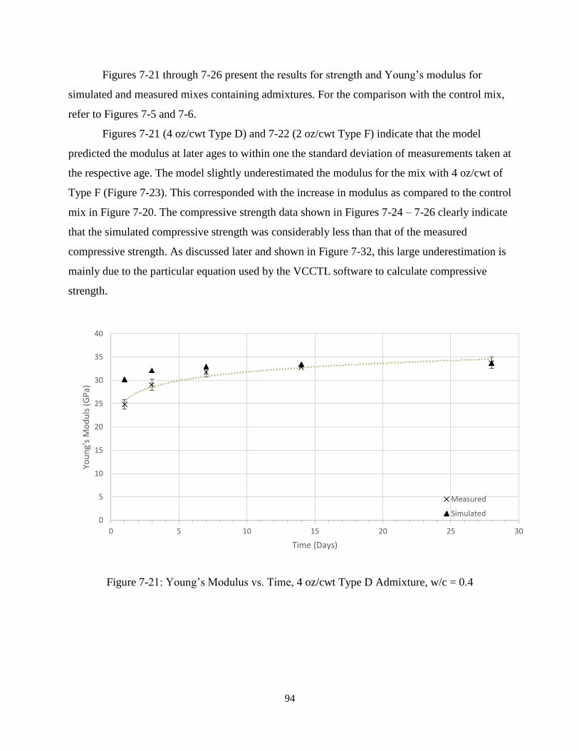
94
Figures 7-21 through 7-26 present the results for strength and Young’s modulus for
simulated and measured mixes containing admixtures. For the comparison with the control mix,
refer to Figures 7-5 and 7-6.
Figures 7-21 (4 oz/cwt Type D) and 7-22 (2 oz/cwt Type F) indicate that the model
predicted the modulus at later ages to within one the standard deviation of measurements taken at
the respective age. The model slightly underestimated the modulus for the mix with 4 oz/cwt of
Type F (Figure 7-23). This corresponded with the increase in modulus as compared to the control
mix in Figure 7-20. The compressive strength data shown in Figures 7-24 – 7-26 clearly indicate
that the simulated compressive strength was considerably less than that of the measured
compressive strength. As discussed later and shown in Figure 7-32, this large underestimation is
mainly due to the particular equation used by the VCCTL software to calculate compressive
strength.
Figure 7-21: Young’s Modulus vs. Time, 4 oz/cwt Type D Admixture, w/c = 0.4
0
5
10
15
20
25
30
35
40
0 5 10 15 20 25 30
You
ng'
s M
od
uls
(G
Pa)
Time (Days)
Measured
Simulated
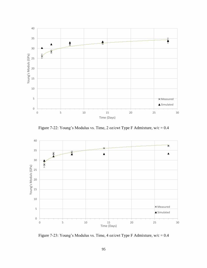
95
Figure 7-22: Young’s Modulus vs. Time, 2 oz/cwt Type F Admixture, w/c = 0.4
Figure 7-23: Young’s Modulus vs. Time, 4 oz/cwt Type F Admixture, w/c = 0.4
0
5
10
15
20
25
30
35
40
0 5 10 15 20 25 30
You
ng'
s M
od
uls
(G
Pa)
Time (Days)
Measured
Simulated
0
5
10
15
20
25
30
35
40
0 5 10 15 20 25 30
You
ng'
s M
od
uls
(G
Pa)
Time (Days)
Measured
Simulated
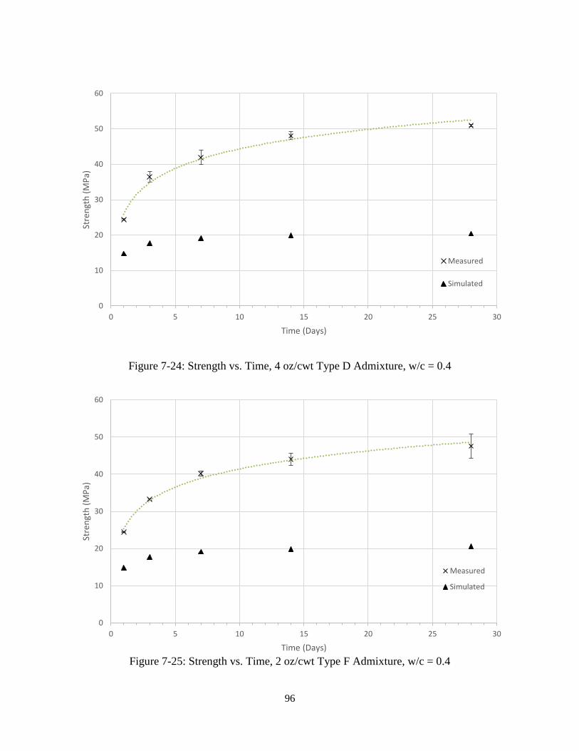
96
Figure 7-24: Strength vs. Time, 4 oz/cwt Type D Admixture, w/c = 0.4
Figure 7-25: Strength vs. Time, 2 oz/cwt Type F Admixture, w/c = 0.4
0
10
20
30
40
50
60
0 5 10 15 20 25 30
Stre
ngt
h (
MP
a)
Time (Days)
Measured
Simulated
0
10
20
30
40
50
60
0 5 10 15 20 25 30
Stre
ngt
h (
MP
a)
Time (Days)
Measured
Simulated
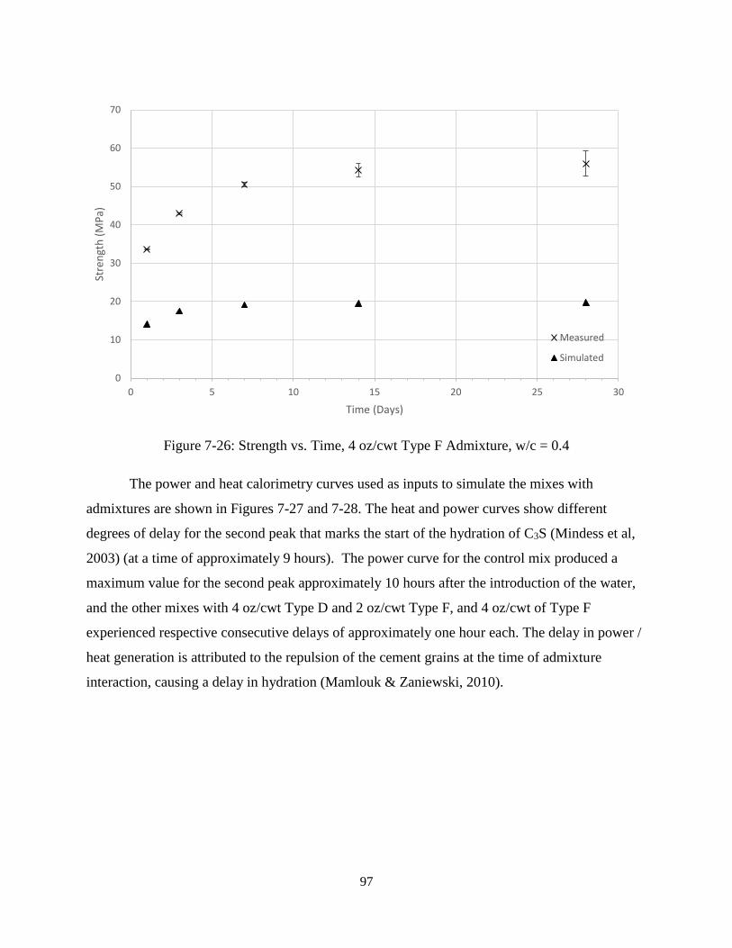
97
Figure 7-26: Strength vs. Time, 4 oz/cwt Type F Admixture, w/c = 0.4
The power and heat calorimetry curves used as inputs to simulate the mixes with
admixtures are shown in Figures 7-27 and 7-28. The heat and power curves show different
degrees of delay for the second peak that marks the start of the hydration of C3S (Mindess et al,
2003) (at a time of approximately 9 hours). The power curve for the control mix produced a
maximum value for the second peak approximately 10 hours after the introduction of the water,
and the other mixes with 4 oz/cwt Type D and 2 oz/cwt Type F, and 4 oz/cwt of Type F
experienced respective consecutive delays of approximately one hour each. The delay in power /
heat generation is attributed to the repulsion of the cement grains at the time of admixture
interaction, causing a delay in hydration (Mamlouk & Zaniewski, 2010).
0
10
20
30
40
50
60
70
0 5 10 15 20 25 30
Stre
ngt
h (
MP
a)
Time (Days)
Measured
Simulated

98
Figure 7-27: Power vs. Time
Figure 7-28: Energy vs. Time
The simulated fraction of solids connected for mixtures which incorporate admixtures is
presented in Figure 7-29. The simulations incorporate the results of heat of hydration (isothermal
calorimetry) results obtained in the laboratory as shown in Figures 7-27 and 7-28. The curves in
Figure 7-29 provided by the simulation indicate that the rate of the connectivity of the solids
0
2
4
6
8
10
12
14
16
18
20
0 5 10 15 20 25 30 35
Po
wer
(m
w/g
)
Time (hours)
No Admixture
4 oz/cwt Type D
2 oz/cwt Type F
4 oz/cwt Type F
0
50
100
150
200
250
300
0 10 20 30 40 50 60 70
Ener
gy (
J/g)
Time (hours)
No Admixture4 oz/cwt Type D2 oz/cwt Type F4 oz/cwt Type F
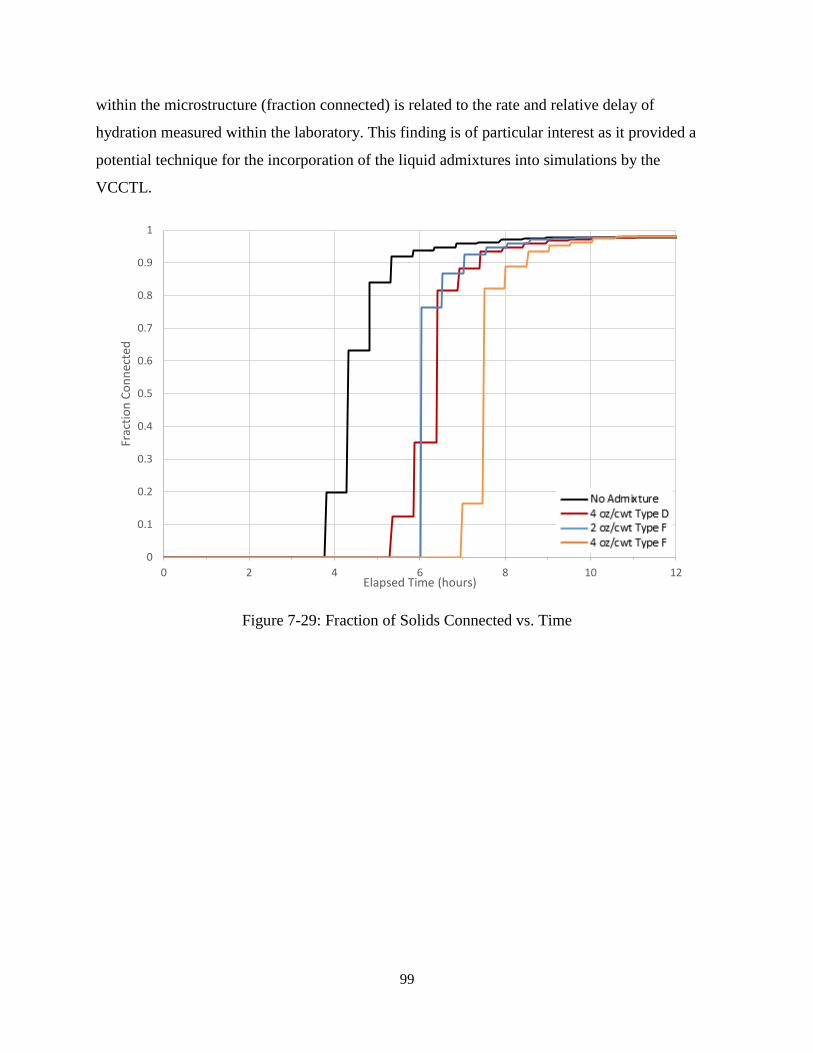
99
within the microstructure (fraction connected) is related to the rate and relative delay of
hydration measured within the laboratory. This finding is of particular interest as it provided a
potential technique for the incorporation of the liquid admixtures into simulations by the
VCCTL.
Figure 7-29: Fraction of Solids Connected vs. Time
0
0.1
0.2
0.3
0.4
0.5
0.6
0.7
0.8
0.9
1
0 2 4 6 8 10 12
Frac
tio
n C
on
nec
ted
Elapsed Time (hours)

100
Figure 7-30: Penetration Resistance vs. Time, Different Admixtures and Dosages
The time of set via penetration resistance testing for the different mixes is presented in
Figure 7-30. The results of the time of set testing indicate that the control mix and mixes with
Type F admixture are in agreement with the results obtained in the isothermal calorimetry
testing, which the exception of the Type D admixture (which incurred a longer delay of set time).
The connectivity of solids, as obtained from the simulation, experienced a delay respective to the
time of set as well. Thus, isothermal calorimetry and time of set testing provide potential input
parameters for VCCTL for concrete mixtures which incorporate liquid admixtures. More
research is need to confirm this theory.
Discussion of Results
Modulus of Elasticity and Compressive Strength
The results from the w/c study mixes and simulations indicate that the VCCTL
software makes reasonable predictions of modulus at a w/c of 0.4, with progressively more
overestimation of modulus as the w/c increases.
0
1000
2000
3000
4000
5000
6000
1.0 2.0 3.0 4.0 5.0 6.0 7.0 8.0
Pen
etra
tio
n R
esis
tan
ce (
psi
)
Elapsed Time (hours)
Effect of Admixtures on Penetration Resistance, 0.4 w/c
Control
4 oz/cwt Type D
2 oz/cwt Type F
4 oz/cwt Type F
Final Set
Initial Set
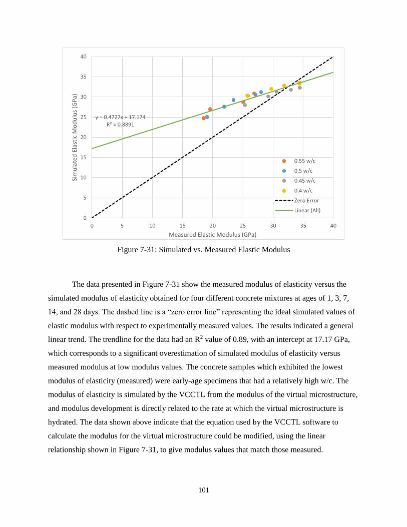
101
Figure 7-31: Simulated vs. Measured Elastic Modulus
The data presented in Figure 7-31 show the measured modulus of elasticity versus the
simulated modulus of elasticity obtained for four different concrete mixtures at ages of 1, 3, 7,
14, and 28 days. The dashed line is a “zero error line” representing the ideal simulated values of
elastic modulus with respect to experimentally measured values. The results indicated a general
linear trend. The trendline for the data had an R2 value of 0.89, with an intercept at 17.17 GPa,
which corresponds to a significant overestimation of simulated modulus of elasticity versus
measured modulus at low modulus values. The concrete samples which exhibited the lowest
modulus of elasticity (measured) were early-age specimens that had a relatively high w/c. The
modulus of elasticity is simulated by the VCCTL from the modulus of the virtual microstructure,
and modulus development is directly related to the rate at which the virtual microstructure is
hydrated. The data shown above indicate that the equation used by the VCCTL software to
calculate the modulus for the virtual microstructure could be modified, using the linear
relationship shown in Figure 7-31, to give modulus values that match those measured.
y = 0.4727x + 17.174R² = 0.8891
0
5
10
15
20
25
30
35
40
0 5 10 15 20 25 30 35 40
Sim
ula
ted
Ela
stic
Mo
du
lus
(GP
a)
Measured Elastic Modulus (GPa)
0.55 w/c
0.5 w/c
0.45 w/c
0.4 w/c
Zero Error
Linear (All)

102
As discussed earlier, the heat of hydration data, as obtained via isothermal calorimetry,
was used as a VCCTL input to provide a timeline to synchronize the rate of simulated
microstructural development and corresponding heat release with measured values.
Regardless of the w/c or whether measured heat of hydration data was used for model
calibration, the simulations of early-age modulus did not produce the level of accuracy as
compared to later ages. Simulated moduli of elasticity at later ages were more comparable to
measured values, with 28-day simulated values within five GPa of the measured values for each
of the concrete mixtures. The exact cause of early-age discrepancies is difficult to determine
directly; more research into the problem is required to illuminate the underlying reasons for this
deficiency. When the cause is determined, investigations into potential corrections to the model
can be performed.
The most obvious discrepancies between simulated and measured values occurred for
strength. Strength was dramatically underestimated by the VCCTL software in all cases.
Simulated modulus values were calculated from a simple empirical relationship. Figure 7-32
shows the relationship between modulus and strength for both simulated and measured values.
Figure 7-32: Strength vs. Elastic Modulus with VCCTL Software Power Fit and ACI 318
As previously discussed, Figures 7-24 – 7-26 provided results in which predicted
compressive strengths obtained from the simulations were considerably underestimated with
y = 0.0504x1.9455
y = 0.0006x2.9674
0
10
20
30
40
50
60
70
80
0 5 10 15 20 25 30 35 40 45
Sren
gth
(M
Pa)
Elastic Modulus (GPa)
MeasuredSimulatedACI 318Power (Measured)

103
respect to compressive strengths as obtained from the specimens tested in the laboratory.
However, the discrepancy between simulated and measured compressive strength is due to the
equation used calculate compressive strength from elastic modulus. The VCCTL uses empirical
equations to calculate compressive strength from simulated modulus of elasticity. Equation 7-1 is
the built-in equation for the VCCTL and originates from work performed by another member of
the VCCTL consortium; however, no publications exist detailing the materials used in the
concrete testing program from which this equation was developed. Equation 7-1 does not come
close to fitting the actual data. Equation 7-2 provides the conversion from elastic modulus to
compressive strength (in metric units) as per ACI 318 (Neville, 2011), and it can be seen that this
equation fits the data fairly well. The best fit, calculated from the data, is given by Equation 7-3,
and can be compared with the other two in Figure 7-32. Use of this equation in the VCCTL
software for the conversion of compressive strength from elastic modulus would definitely
improve the accuracy of the simulated values.
𝑓𝑐′ = 0.0006𝐸𝑐
2.9674 (7-1)
𝑓𝑐′ = 0.0447𝐸𝑐
2 (7-2)
𝑓𝑐′ = 0.0504𝐸𝑐
1.9455 (7-3)
Where:
Ec is modulus of elasticity in GPa and
f’c is compressive strength in MPa
Though the relationship defined in ACI 318 appears as though it would predict strength
fairly well at later ages in this circumstance, the use of empirical relationships does not take into
account many of the factors that influence the behavior of concrete. It is possible that the
discrepancy between the VCCTL software’s predictions and the actual physical results is due to
one of these factors, the most likely of which being the scenario in which the coarse aggregates
being modeled do not have the same properties as those of the materials used to develop the
empirical relationship.
Due to the lack of information on the materials used to develop the empirical relationship
between modulus and strength, any possible explanation for the drastic underprediction of

104
strength for the concrete used in this study must come from specific knowledge about the
properties of the materials used as well as an assumption about the nature of the materials used to
establish the equation 7-1.
The concrete in this study exhibited fracture behavior that corresponds to the commonly
described mechanism of failure for concrete. Typical concrete fails in compression when
microcracks initiated at the interfacial transition zones surrounding aggregates propagate through
the specimen, resulting in failure planes that pass around aggregate particles (Maso, 1996). This
is called intergranular fracture. In the concrete used in this study however, the failure planes
passed through the aggregate particles, commonly referred to as transgranular fracture. Figure 7-
33 shows an example of a failed cylinder that exhibits this behavior. Coarse aggregate particles
that have fractured are clearly visible in the two fragments as shown in Figure 7-33. An
aggregate particle face in one fragment is mirrored in the other fragment, which came from the
opposite side of the failure plane. Based on this phenomenon, it can be concluded that the
strength of the interfacial transition zone in the concrete used in this research is sufficient to
cause fracture to occur through the grain rather than through the interfacial transition zone.
Factors favoring transgranular fracture are better bonding between the aggregate and
paste, weaker aggregate, or some combination of these two factors. The coarse aggregate used in
this study was observably porous and angular, with an absorption of approximately 4.5%. The
diffusion of hydration products into porous aggregates, which are initially saturated (all
aggregate was in a saturated state) as well as the mechanical interlock between the cement paste
and irregular aggregate surfaces can strengthen the interfacial transition zone to the point where
it is no longer vulnerable to microcrack propagation (Maso, 1996). It has also been observed
petrographically that the rough surfaces of Florida limestone (also referred to as limerock)
aggregates provide good mechanical interlock and exhibit chemical bonding with cement paste
(McClellan, et al., 1993).
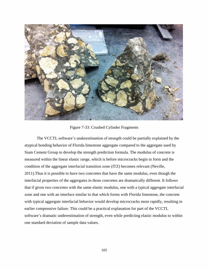
105
Figure 7-33: Crushed Cylinder Fragments
The VCCTL software’s underestimation of strength could be partially explained by the
atypical bonding behavior of Florida limestone aggregate compared to the aggregate used by
Siam Cement Group to develop the strength prediction formula. The modulus of concrete is
measured within the linear elastic range, which is before microcracks begin to form and the
condition of the aggregate interfacial transition zone (ITZ) becomes relevant (Neville,
2011).Thus it is possible to have two concretes that have the same modulus, even though the
interfacial properties of the aggregates in those concretes are dramatically different. It follows
that if given two concretes with the same elastic modulus, one with a typical aggregate interfacial
zone and one with an interface similar to that which forms with Florida limestone, the concrete
with typical aggregate interfacial behavior would develop microcracks more rapidly, resulting in
earlier compressive failure. This could be a practical explanation for part of the VCCTL
software’s dramatic underestimation of strength, even while predicting elastic modulus to within
one standard deviation of sample data values.

106
Model Sensitivity
The results of the investigation into the sensitivity of the model to the presence of
different material input data show that several of the non-essential input values have little
influence on the outcome of simulations. Aggregate shape data, while documented to have an
influence on the strength of concrete (Jones & Kaplan, 1957), has no effect on the simulated
strength because it has no effect on elastic modulus, the value from which strength is calculated.
The size of the simulated microstructure had a very slight effect on the results of simulations in
this case, though even a small increase in size results in a dramatic increase in simulation
computing time.
The influence of aggregate elastic properties on the elastic properties of the concrete is
substantial. The aggregate makes up a large fraction of the concrete by volume, and the VCCTL
software calculates the modulus of the concrete based on the computed modulus of the paste as
well as the relative volume fractions and elastic properties of the coarse and fine aggregate.
The absence of isothermal calorimetry data resulted in an underestimation of modulus, as
opposed to an overestimation of modulus when calorimetry data was used as an input parameter
for the simulated concrete. The absence of cement particle shape data had no appreciable
influence on modulus, but had a similar effect on set time as the absence of calorimetry data. It is
possible that if both of these inputs were missing the effect on set time could be compounded.
Admixture Influence on Set Time
The simulation of the delay in set time due to admixtures, by using isothermal
calorimetry data obtained from those admixtures, was a partial success. The predicted delay in
set time of the mixes containing two different dosage rates of Type F matched up with the
measured set time delay of the actual concrete. The mix containing Type D did not however,
with the predicted set occurring in roughly half the time of the actual measured set. Heat
evolution and set time of concrete are two individual phenomena, and while they may be linked,
the beginning of one does not necessarily imply the start of the other.

107
CHAPTER 8 CONCLUSIONS AND RECOMMENDATIONS
Conclusions
The results of this research led to the following conclusions about the VCCTL software:
1. The VCCTL software was found to be an effective tool for the simulation of elastic
modulus of portland cement concrete, provided the materials being simulated are
properly characterized.
2. At the current stage of development, the VCCTL software did not accurately predict the
compressive strength of portland cement concrete using Florida limestone coarse
aggregate. This is expected to be resolved by improving the accuracy of the raw material
property inputs, and by making modifications to the software programming.
3. The VCCTL software currently does not have a means to incorporate the effects of
admixtures on cement hydration. An initial attempt to integrate the effects of a water-
reducing admixture, using heat of hydration data, was successful for Type F water
reducer, but the software underestimated the setting time for Type D water reducer.
Further research should be performed to reliably incorporate the effects of admixtures
into the VCCTL.
4. The process of acquiring cement phase volume and surface area fraction data has been
improved substantially through the use of automated scanning electron microscopy. This
has resulted in a more efficient process to obtain cement characterization data for use in
the VCCTL software.
5. The empirical predictions for compressive strength, which are based on elastic modulus
and developed for concretes using coarse aggregates that were mineralogically and/or
microstructurally different than typical Florida limestone aggregates, were not accurate
for concretes made with Florida limestone. More research is needed to accurately predict
the compressive strength based on the elastic properties of concrete containing Florida
limestone coarse aggregates for different concrete mixtures.
6. Comparison of isothermal calorimetry data and corresponding time of set data has shown
that a typical Type F high-range water-reducing admixture (superplasticizer) delayed
time of set and shifted the main silicate hydration peak by the same amount of time. At
the dosages explored within this study, the delay was proportional to the dosage rate.
108
7. Higher dosage rates of Type F high-range water-reducing admixture (superplasticizer)
typically resulted in an increase in both elastic modulus and compressive strength, when
compared to the control mixes.
Recommendations
Based on the findings from this study, the following recommendations were made:
1. The conclusions drawn from the work performed in this research discovered several
potential topics for future research, both to improve the accuracy of the model as well as
to explore different material inputs and outputs.
2. The empirical compressive strength model built into the VCCTL software, which is
based on elastic modulus, does not accurately predict compressive strength for concrete
mixtures which incorporate well for Florida limestone. Generalized empirical predictions
for strength of concrete are inherently limited due to the variability of the materials used
for production. A more fundamental approach to the simulation of concrete strength
should be investigated.
3. Detailed characterization of the elastic properties of Florida limestones used to produce
coarse aggregates for portland cement concrete should be performed. A database of
properties of concrete mix designs containing Florida aggregate for use with the VCCTL
software and other projects should be created.
4. The VCCTL software supports the modeling of admixtures if the specific phase surface
deactivation behavior of the admixture is known. Methods of obtaining this information,
either through material testing, or possibly from the admixture manufacturer, should be
investigated.
5. There are a number of materials that can be modeled in the VCCTL software that were
not considered for this research. There is support for both fly ash and blast furnace slag
hydration in the VCCTL software, though the accuracy of the model in this respect is
largely unknown. The techniques required to characterize these materials are also more
involved due to the significant glassy (amorphous) phase contents of their compositions.
The methods by which these materials can be characterized and the accuracy with which
they are simulated in the VCCTL software should be explored.
109
LIST OF REFERENCES
ACI Committee 318: “Building Code Requirements for Structural Concrete (ACI 318-11) and
Commentary”, American Concrete Institute, Farmington Hills, MI, 2011, 509 pp.
ASTM C39: ASTM C39-12a, “Standard Test Method for Compressive Strength of Cylindrical
Concrete Specimens”, ASTM International, West Conshohocken, PA, 2012, 7 pp.
ASTM C127: ASTM C127-12, “Standard Test Method for Density, Relative Density (Specific
Gravity), and Absorption of Coarse Aggregate”, ASTM International, West
Conshohocken, PA, 2012, 6 pp.
ASTM C136: ASTM C136-06, “Standard Test Method for the Sieve Analysis of Fine and
Coarse Aggregate”, ASTM International, West Conshohocken, PA, 2006, 5 pp.
ASTM C138: ASTM C138-13, “Standard Test Method for Density (Unit Weight), Yield, and Air
Content (Gravimetric) of Concrete”, ASTM International, West Conshohocken, PA,
2013, 4 pp.
ASTM C143: ASTM C143-12, “Standard Test Method for Slump of Hydraulic-Cement
Concrete”, ASTM International, West Conshohocken, PA, 2012, 4 pp.
ASTM C150: ASTM C150-12, “Standard Specification for Portland Cement”, ASTM
International, West Conshohocken, PA, 2012, 9 pp.
ASTM C173: ASTM C173-12, “Standard Test Method for Air Content of Freshly Mixed
Concrete by the Volumetric Method”, ASTM International, West Conshohocken, PA,
2012, 9 pp.
ASTM C186: ASTM C186-05, “Standard Test Method for Heat of Hydration of Hydraulic
Cement”, ASTM International, West Conshohocken, PA, 2005, 7 pp.
ASTM C192: ASTM C192-13, “Standard Practice for Making and Curing Concrete Test
Specimens in the Laboratory”, ASTM International, West Conshohocken, PA, 2013, 8
pp.
ASTM C204: ASTM C204-11, “Standard Test Method for Fineness of Hydraulic Cement by
Air-Permeability”, ASTM International, West Conshohocken, PA, 2011, 9 pp.
ASTM C403: ASTM C403-08, “Standard Test Method for Time of Setting of Concrete Mixtures
by Penetration Resistance”, ASTM International, West Conshohocken, PA, 2008, 7 pp.
ASTM C469: ASTM C469-10, “Standard Test Method for Static Modulus of Elasticity and
Poisson’s Ratio of Concrete in Compression”, ASTM International, West Conshohocken,
PA, 2010, 5 pp.
ASTM C566: ASTM C566-13, “Standard Test Method for Total Moisture Content of Aggregate
by Drying”, ASTM International, West Conshohocken, PA, 2013, 3 pp.

110
ASTM C1064: ASTM C1064-12, “Standard Test Method for Temperature of Freshly Mixed
Hydraulic-Cement Concrete”, ASTM International, West Conshohocken, PA, 2012, 3 pp.
ASTM C1365: ASTM C1365-06, Reapproved 2011, “Standard Test Method for Determination
of the Proportion of Phases in Portland Cement and Portland-Cement Clinker Using X-
Ray Powder Diffraction Analysis”, ASTM International, West Conshohocken, PA, 2006,
10 pp.
ASTM C1702: ASTM C1702-13, “Standard Test Method for Measurement of Heat of Hydration
of Hydraulic Cementitious Materials Using Isothermal Conduction Calorimetry”, ASTM
International, West Conshohocken, PA, 2013, 8 pp.
Bentz 2005: Bentz, D. P. (2005). “Quantitative Comparison of Real and CEMHYD3D Model
Microstructures Using Correlation Functions”. Cement and Concrete Research, 36(2),
259-263.
Bentz 2006: Bentz, D. P. (2006). “Modeling the Influence of Limestone Filler on Cement
Hydration Using CEMHYD3D”. Cement and Concrete Composites, 28(2), 124-129.
Bentz et al. 2000: Bentz, D. P., Feng, X., Haecker, C.-J., and Stutzman, P. E. (2000). “Analysis
of CCRL Proficiency Cements 135 and 136 Using CEMHYD3D (NIST Report NISTIR
6545, August 2000)”. National Institute of Standards and Technology, Gaithersburg, MD.
Available online at http://fire.nist.gov/bfrlpubs/build00/PDF/b00097.pdf.
Bentz et al. 2003: Bentz, D. P., Haecker, C., Feng, X., and Stutzman, P. (2003). “Prediction of
Cement Physical Properties by Virtual Testing”. Process Technology of Cement
Manufacturing, Proceedings of the Fifth International VDZ Congress, September 23-27,
2002. VDZ gGmbH, Düsseldorf, Germany, 53-63.
Bullard 2002: Bullard, J. W. (2002). “Curing of Concrete: Spatial and Temporal Randomness
Over Multiple Length Scales”. PowerPoint Presentation Given May 1, 2002 at Holcim,
Dundee, MI.
Bullard and Garboczi 2006: Bullard, J. W., and Garboczi, E. J. (2006). “A Model Investigation
of the Influence of Particle Shape on Portand Cement Hydration”. Cement and Concrete
Research, 36(6) 1007-1015.
Bullard and Obla 2004: Bullard, J. W., and Obla, K. (2004). “Virtual Testing of Ready Mixed
Concrete”. Concrete inFocus, 3(1), 38-41.
Bullard et al. 2013: Bullard, J., Garboczi, E., and Stutzman, P. (2013). “VCCTL Software:
Overview and Opportunities”. Industry Application of the Virtual Cement and Concrete
Library Webinar, June 3, 2013, Sponsored by RMC Research and Education Foundation,
Silver Spring, MD. Available online at http://www.rmc-foundation.org/images/VCCTL-
Webinar-Bullard.pdf.
CSHub 2014: Concrete Sustainability Hub. Access website at: http://cshub.mit.edu/.

111
Edmeades and Hewlett 1998: Edmeades, R. M., and Hewlett, P. C. (1998). “Cement
Admixtures”, Chapter 12, pp. 841-905 in Lea's Chemistry of Cement and Concrete,
Elsevier, Oxford, UK.
Elwell and Fu 1995: Elwell, D. J., and Fu, G. (1995). “Compression Testing of Concrete:
Cylinders vs. Cubes”. Special Report Volume 119, Transportation Research and
Development Bureau, New York State Department of Transportation, 22 pp.
FDOT 2014: Florida Department of Transportation. (2014). “Portland Cement Concrete”. pp.
308-328 in Standard Specifications for Road and Bridge Construction, FDOT,
Tallahassee, FL.
Feng et al. 2004: Feng, X., Garboczi, E. J., Bullard, J. W., Bentz, D. P., Snyder, K. A., Stutzman,
P. E., and Mason, T. O. (2004). “Expanding a Tool for Predicting Chloride Diffusivity in
Concrete So It Can Be Used by Manufacturers to Evaluate the Durability of Concrete
Made With Blended Cements. Part I: Characterizing Blended Cement Materials (NIST
Report NISTIR 7135, August 2004)”, National Institute of Standards and Technology,
Gaithersburg, MD.
Ferraro 2009: Ferraro, C. C. (2009). “Determination of Test Methods for the Prediction of the
Behavior of Mass Concrete”. Ph.D. Thesis, University of Florida, Gainesville, FL.
Garboczi and Bentz 1998: Garboczi, E. J., and Bentz, D. P. (1998). “The Microstructure of
Portland Cement-Based Materials: Computer Simulation and Percolation Theory”. pp.
89-100 in Computational and Mathematical Models of Microstructural Evolution,
Materials Research Society Symposium Proceedings, Volume 529, San Francisco,
California, April 13-17, 1998, Materials Research Society, Warrendale, PA.
Garboczi and Berryman 2001: Garboczi, E., and Berryman, J. (2001). “Elastic Moduli of a
Material Containing Composite Inclusions: Effective Medium Theory and Finite Element
Computations”. Mechanics of Materials, 33(8), 455-470.
Garboczi and Day 1995: Garboczi, E. J., and Day, A. R. (1995). “An Algorithm for Computing
the Effective Linear Elastic Properties of Heterogeneous Materials: Three-Dimensional
Results for Composites with Equal Phase Ratios”. Journal of the Mechanical Physics of
Solids, 43(9), 1349-1362.
Garboczi et al. 1991: Garboczi, E. J., Thorpe, M. F., and Day, A. R. (1991). “Universal
Conductivity Curves for a Plane Containing Random Holes”. Physical Review A, 43(12),
6473-6482.
Garboczi et al. 2000: Garboczi, E. J, Bentz, D. P., and Frohnsdorff, G. J.. (2000). “The Past,
Present and Future of Computational Materials Science of Concrete”. Reprinted from
Materials Science of Concrete Workshop Proceedings (April 27-29, 2000, in honor of J.
Francis Young). Center for Advanced Cement-Based Materials (ACBM), April 27-29,
2000, Lake Shelbyville, IL.
112
Garboczi et al. 2004: Garboczi, E. J., Bullard, J. W., and Bentz, D. P. (2004). “Virtual Testing of
Cement and Concrete - USA 2004”. Concrete International, 26(12), 33-37.
Garboczi et al. 2010: Garboczi, E., Bullard, J., and Martys, N. (2010). “The Virtual Cement and
Concrete Testing Laboratory: Application to Sustainability”. Presented at the Concrete
Sustainability Conference, April 13-15, 2010, Tempe, AZ, Sponsored by the National
Ready Mixed Concrete Association, Silver Spring, MD.
Goldstein et al. 2007: Goldstein, J., Newberry, D. E., Joy, D. C., Lyman, C. E., Echlin, P.,
Lifshin, E., and Michael, J. (2007). Scanning Electron Microscopy and X-Ray
Microanalysis, Springer, New York, NY.
Jennings and Johnson 1986: Jennings, H. N. and Johnson, S. K. (1986). “Simulation of
Microstructure Development During the Hydration of of a Cement Compound.” J. Am.
Ceram. Soc., 69(11) 790-799.
Jones and Kaplan 1957: Jones, R., and Kaplan, M. F. (1957). “The Effects of Coarse Aggregate
on the Mode of Failure of Concrete in Compression and Flexure”. Magazine of Concrete
Research, 9(26), 89-94.
Mamlouk and Zaniewski 2010: Mamlouk, M. C., and Zaniewski, J. P. (2010). Materials for Civil
and Construction Engineers. Prentice Hall, Upper Saddle River, NJ.
Maso 1996: Maso, J. C. (1996). “Influence of the Interfacial Transition Zone on Composite
Mechanical Properties”. pp. 114-129 in Interfacial Transition Zone in Concrete, Rilem
Report 11, E & FN Spon, London, UK.
McClellan et al. 1993: McClellan, G. H., Eades, J. L., and Fountain, K. B. (1993). “Petrographic
Characteristics of Florida Limestone Aggregates used in Concrete - Phase II. Final
Report”. University of Florida, Dept. of Geology, Gainesville, FL.
Mindess and Young 1981: Mindness, S., and Young, J. F. (1981). Concrete, Prentice-Hall, Inc.,
Englewood Cliffs, NJ.
Mindess and Young 2003: Mindess, S., Young, J. F., and Darwin, D. (2003). Concrete, Second
Edition, Prentice-Hall, Inc., Upper Saddle River, NJ.
Neville 2012: Neville, A. M. (2012). Properties of Concrete, Fifth Edition. Trans-Atlantic
Publications, Inc., Philadelphia, PA.
Peyrot 2006: Peyrot, I. C. (2006). “Development and Validation of a 3D Computational Tool to
Describe Damage and Fracture due to Alkali Silica Reaction in Concrete Structures”.
Ph.D. Thesis, Paris School of Mines, Alès, France.
Russo 2012: Russo, V. (2012). “Towards a Modelization of the Effect of Superplasticizers on
Early-Age Mechanical Strengths with VCCTL”. Presentation given at the Fall 2012
VCCTL Consortium Meeting, December 13, 2012, Florida Department of Transportation
State Materials Office, Gainesville, FL.

113
Sahachaiyunta 2012: Sahachaiyunta, P., Pongpaisanseree, K., Bullard, J. W., Stutzman, P. E.,
Garboczi, E. J., and Vichit-Vadakan, W. (2012). “Virtual Testing in a Cement Plant”.
Concrete International, 34(9), 33-39.
Valentini 2013: Valentini, L., Parisatto, M., Russo, V., Ferrari, G., Bullard, J. W., Angel, R. J.,
and Artoli, G. (2013). “Prediction of the Properties of Industrial Cement Mortars by
Computer Modeling” (preprint). Science and Technology of Advanced Materials, in
press.
Waseda et al. 2011: Waseda, Y., Matsubara, E., and Shinoda, K. (2011). X-Ray Diffraction
Crystallography: Introduction, Examples and Solved Problems. Springer, Heidelberg,
DE.
Watts et al. 2013: Watts, B., Ferraro, C., Snyder, A., and DeFord, H. D. (2013). “Automated and
Manual Characterization of Input Parameters for the VCCTL”. Presented at the 4th
Advances in Cement-Based Materials: Characterization, Processing, Modeling and
Sensing, July 8-10, Champaign, Illinois.
Wittke 2008: Wittke, J. H. (2008). “Signals”. Available online at
http://www4.nau.edu/microanalysis/Microprobe-SEM/Signals.html.
Wittman et al. 1985: Wittmann, F. H., Roelfstra, P. E., and Sadouki, H. (1985). “Simulation and
Analysis of Composite Structures.” Materials Science and Engineering, 68(2) 239-248.
Zienkiewicz et al. 2005: Zienkiewicz, O. C., Taylor, R. L., and Zhu, J. Z. (2005). The Finite
Element Method: Its Basis and Fundamentals, Sixth Edition. Elsevier Butterworth-
Heinemann, Burlington, MA.

114
APPENDIX A
MATHEMATICAL EQUATIONS REFERENCE FOR THE CALCULATION OF ELASTIC
MODULI USING DIFFERENTIAL EFFECTIVE MEDIUM THEORY
The equations used to create a single effective particle are as follows
2𝐴(𝐺/𝐺2) + 2𝐵(𝐺/𝐺2) + 𝐶 = 0
Where:
𝐴 = 8𝑧(4 − 5𝜈2)𝜂𝛼𝑝103 − 2[63𝑧𝜂𝛽 + 2𝜂𝛼𝜂𝛽]𝑝
73 + 252𝑧𝜂𝛽𝑝
53 − 50𝑧(7 − 12𝜈2 + 8𝜈2
2)𝜂𝛽𝑝5/3
+ 4(7 − 10𝜈2)𝜂𝛾𝛼𝜂𝛽
𝐵 = −2𝑧(1 − 5𝜈2)𝜂𝛼𝑝103 − 2[63𝑧𝜂𝛽 + 2𝜂𝛼𝜂𝛾]𝑝
73 − 252𝑧𝜂𝛽𝑝
53 + 75𝑧(3 − 𝜈2)𝜂𝛽𝜈2𝑝
+ 3/2(15𝜈2 − 7)𝜂𝛾𝛼𝜂𝛽
𝐶 = 4𝑧(5𝜈2 − 7)𝜂𝛼𝑝103 − 2[63𝑧𝜂𝛽 + 2𝜂𝛼𝜂𝛾]𝑝
73 + 252𝑧𝜂𝛽𝑝
53 + 25𝑧(𝜈2
2 − 7)𝜂𝛽𝑝 + (7
− 5𝜈2)𝜂𝛼𝛽𝜂𝛽
G = The effective shear modulus
K = The effective bulk modulus, given by:
𝐾 = 𝐾2 +𝑐(𝐾3 − 𝐾2)
1 + (1 − 𝑐)𝐾3 − 𝐾2
𝐾2 +43 𝐺2
The differential equations used to solve numerically for the composite modulus are as follows
𝑑𝐾
𝑑∅= −𝑘𝐾/∅
𝑑𝐺
𝑑∅= −𝑔𝐺/∅
Where

115
𝑘 =(𝐾𝑚 +
43 𝐺𝑚)(𝐾𝑝 + 𝐾𝑚)
𝐾𝑚(𝐾𝑝 +43 𝐺𝑚)
𝑔 =(𝐾𝑚 +
43 𝐺𝑚)(𝐺𝑝 + 𝐺𝑚)
3𝐺𝑚 (𝐾𝑚 +89 𝐺𝑚) + 2𝐺𝑝(𝐾𝑚 + 2𝐺𝑚)
m = Specified property of the matrix, and
p = Specified property of the particle.
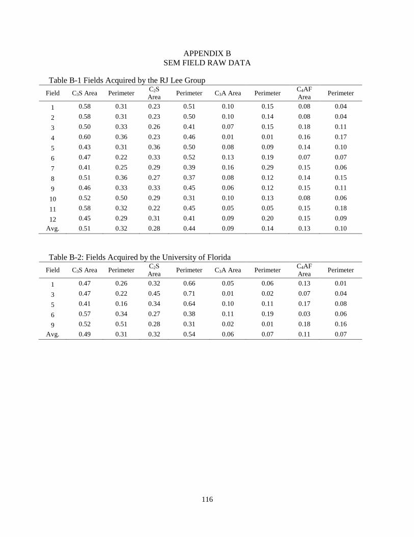
116
APPENDIX B
SEM FIELD RAW DATA
Table B-1 Fields Acquired by the RJ Lee Group
Field C3S Area Perimeter C2S
Area Perimeter C3A Area Perimeter
C4AF
Area Perimeter
1 0.58 0.31 0.23 0.51 0.10 0.15 0.08 0.04
2 0.58 0.31 0.23 0.50 0.10 0.14 0.08 0.04
3 0.50 0.33 0.26 0.41 0.07 0.15 0.18 0.11
4 0.60 0.36 0.23 0.46 0.01 0.01 0.16 0.17
5 0.43 0.31 0.36 0.50 0.08 0.09 0.14 0.10
6 0.47 0.22 0.33 0.52 0.13 0.19 0.07 0.07
7 0.41 0.25 0.29 0.39 0.16 0.29 0.15 0.06
8 0.51 0.36 0.27 0.37 0.08 0.12 0.14 0.15
9 0.46 0.33 0.33 0.45 0.06 0.12 0.15 0.11
10 0.52 0.50 0.29 0.31 0.10 0.13 0.08 0.06
11 0.58 0.32 0.22 0.45 0.05 0.05 0.15 0.18
12 0.45 0.29 0.31 0.41 0.09 0.20 0.15 0.09
Avg. 0.51 0.32 0.28 0.44 0.09 0.14 0.13 0.10
Table B-2: Fields Acquired by the University of Florida
Field C3S Area Perimeter C2S
Area Perimeter C3A Area Perimeter
C4AF
Area Perimeter
1 0.47 0.26 0.32 0.66 0.05 0.06 0.13 0.01
3 0.47 0.22 0.45 0.71 0.01 0.02 0.07 0.04
5 0.41 0.16 0.34 0.64 0.10 0.11 0.17 0.08
6 0.57 0.34 0.27 0.38 0.11 0.19 0.03 0.06
9 0.52 0.51 0.28 0.31 0.02 0.01 0.18 0.16
Avg. 0.49 0.31 0.32 0.54 0.06 0.07 0.11 0.07