final report on: magnetotelluric and … report on: magnetotelluric and audiomagnetotelluric surveys...
TRANSCRIPT

Final Report on:
Magnetotelluric and AudioMagnetotelluric Surveys on
Department of Hawaiian Home Lands
Mauna Kea East Flank
Submitted By:
Donald Thomas
Hawaii Institute of Geophysics and Planetology
Center for the Study of Active Volcanoes
December 9, 2016

i
Executive Summary
This project has collected electromagnetic and electrical potential data from 70 locations
collected in multiple linear transect intervals along a 28 km section of Mauna Kea’s mid-
elevation eastern flank. The measurements were all made on Department of Hawaiian Home
Lands (DHHL) property that flanks the Mana/Keanakolu Road that runs from the intersection
with the Mauna Kea Observatory Access Road north toward Waimea where it eventually
intersects with Hawaii State 19. The electrical potential and electromagnetic measurements
were made with Magnetotelluric (10 stations) and AudioMagnetotelluric (60 stations)
instruments that allow us to process and model the recovered data to produce a map of the
subsurface electrical resistivity distributions down to depths of more than 10 kilometers below
the ground surface. These electrical resistivity distributions are widely used in the energy and
minerals industries to identify and narrow the search for oil and gas or mineral prospects as
well as for identification of both geothermal and groundwater resource potential. The
collected data have been reviewed and refined to minimize the effects of interfering
electromagnetic noise; inverted using 1D modeling to yield apparent resistivity with depth
curves; and modeled using 2D inversion programs. Electrical resistivity versus depth profiles
have been constructed along the survey transects using both the 1D and 2D modeling results to
yield a resistivity cross section through the east flank of Mauna Kea. These cross sections reveal
three moderate to low resistivity intervals at depths of 3 km or less. All three low resistivity
intervals are interpreted to reflect current or prior thermal activity at shallow depths. The
northern and southern low resistivity intervals are believed to be associated with subsidiary
dike complexes of Mauna Kea and therefore may have limited geothermal potential, whereas
the central resistivity low is, based on both the results of the current surveys as well as
geological analysis, to correspond to a Mauna Kea East Rift Zone that would represent the
highest geothermal resource potential. Analysis of the shallower resistivity distributions along
the composite transect lines suggests that there is also potential for high elevation
groundwater resources in the region that could, if carefully developed, provide a viable water
supply for DHHL lessees.
Additional exploration work that could be pursued to better characterize the prospective
geothermal resource would be additional Magnetotelluric and AudioMagnetotelluric surveys,
as well as gravity surveys, across the postulated rift zone at higher and lower elevations on
Mauna Kea’s east flank. The former work would further confirm the width and extent of the
identified resistivity anomaly whereas the latter would provide an estimate of the volume of
magmatic intrusions within this inferred rift zone and some estimate of the heat content.
1
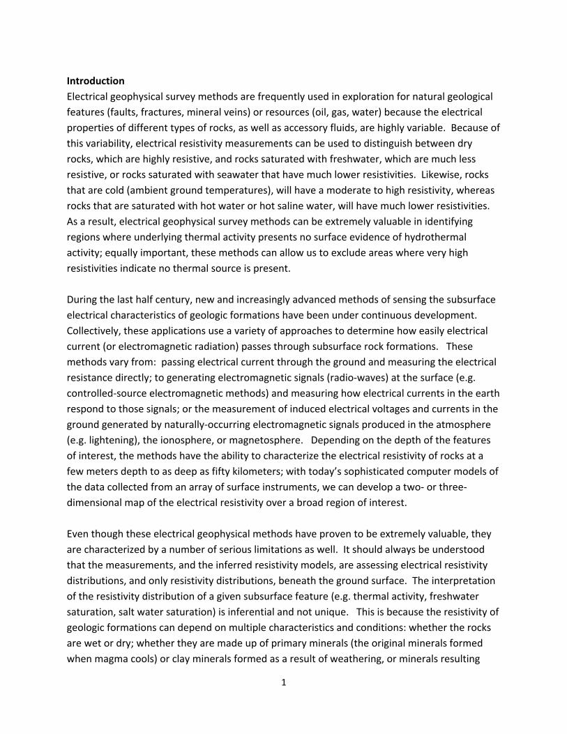
Introduction
Electrical geophysical survey methods are frequently used in exploration for natural geological
features (faults, fractures, mineral veins) or resources (oil, gas, water) because the electrical
properties of different types of rocks, as well as accessory fluids, are highly variable. Because of
this variability, electrical resistivity measurements can be used to distinguish between dry
rocks, which are highly resistive, and rocks saturated with freshwater, which are much less
resistive, or rocks saturated with seawater that have much lower resistivities. Likewise, rocks
that are cold (ambient ground temperatures), will have a moderate to high resistivity, whereas
rocks that are saturated with hot water or hot saline water, will have much lower resistivities.
As a result, electrical geophysical survey methods can be extremely valuable in identifying
regions where underlying thermal activity presents no surface evidence of hydrothermal
activity; equally important, these methods can allow us to exclude areas where very high
resistivities indicate no thermal source is present.
During the last half century, new and increasingly advanced methods of sensing the subsurface
electrical characteristics of geologic formations have been under continuous development.
Collectively, these applications use a variety of approaches to determine how easily electrical
current (or electromagnetic radiation) passes through subsurface rock formations. These
methods vary from: passing electrical current through the ground and measuring the electrical
resistance directly; to generating electromagnetic signals (radio-waves) at the surface (e.g.
controlled-source electromagnetic methods) and measuring how electrical currents in the earth
respond to those signals; or the measurement of induced electrical voltages and currents in the
ground generated by naturally-occurring electromagnetic signals produced in the atmosphere
(e.g. lightening), the ionosphere, or magnetosphere. Depending on the depth of the features
of interest, the methods have the ability to characterize the electrical resistivity of rocks at a
few meters depth to as deep as fifty kilometers; with today’s sophisticated computer models of
the data collected from an array of surface instruments, we can develop a two- or three-
dimensional map of the electrical resistivity over a broad region of interest.
Even though these electrical geophysical methods have proven to be extremely valuable, they
are characterized by a number of serious limitations as well. It should always be understood
that the measurements, and the inferred resistivity models, are assessing electrical resistivity
distributions, and only resistivity distributions, beneath the ground surface. The interpretation
of the resistivity distribution of a given subsurface feature (e.g. thermal activity, freshwater
saturation, salt water saturation) is inferential and not unique. This is because the resistivity of
geologic formations can depend on multiple characteristics and conditions: whether the rocks
are wet or dry; whether they are made up of primary minerals (the original minerals formed
when magma cools) or clay minerals formed as a result of weathering, or minerals resulting
2
from hydrothermal activity (the latter being less resistive than the former); and whether the
rocks are cold or hot (or molten – magma has a very low resistivity). In order to reduce the
uncertainties in interpretation of resistivity results, we frequently conduct resistivity
measurements over a known resource or feature to determine its electrical characteristics
(resistivity) in the geologic environment of interest. Those data serve as reference points when
conducting surveys over nearby regions for which a resource or feature of interest has not been
proven to exist by direct measurement. Even with the baseline or reference measurements,
there is always a degree of uncertainty regarding a resource even when we find matching
resistivity values.
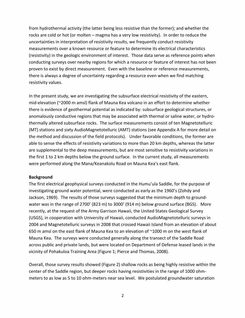
In the present study, we are investigating the subsurface electrical resistivity of the eastern,
mid-elevation (~2000 m amsl) flank of Mauna Kea volcano in an effort to determine whether
there is evidence of geothermal potential as indicated by: subsurface geological structures, or
anomalously conductive regions that may be associated with thermal or saline water, or hydro-
thermally altered subsurface rocks. The surface measurements consist of ten Magnetotelluric
(MT) stations and sixty AudioMagnetotelluric (AMT) stations (see Appendix A for more detail on
the method and discussion of the field protocols). Under favorable conditions, the former are
able to sense the effects of resistivity variations to more than 20 km depths, whereas the latter
are supplemental to the deep measurements, but are most sensitive to resistivity variations in
the first 1 to 2 km depths below the ground surface. In the current study, all measurements
were performed along the Mana/Keanakolu Road on Mauna Kea’s east flank.
Background
The first electrical geophysical surveys conducted in the Humu’ula Saddle, for the purpose of
investigating ground water potential, were conducted as early as the 1960’s (Zohdy and
Jackson, 1969). The results of those surveys suggested that the minimum depth to ground-
water was in the range of 2700’ (823 m) to 3000’ (914 m) below ground surface (BGS). More
recently, at the request of the Army Garrison Hawaii, the United States Geological Survey
(USGS), in cooperation with University of Hawaii, conducted AudioMagnetotelluric surveys in
2004 and Magnetotelluric surveys in 2008 that crossed Hawaii Island from an elevation of about
650 m amsl on the east flank of Mauna Kea to an elevation of ~1000 m on the west flank of
Mauna Kea. The surveys were conducted generally along the transect of the Saddle Road
across public and private lands, but were located on Department of Defense leased lands in the
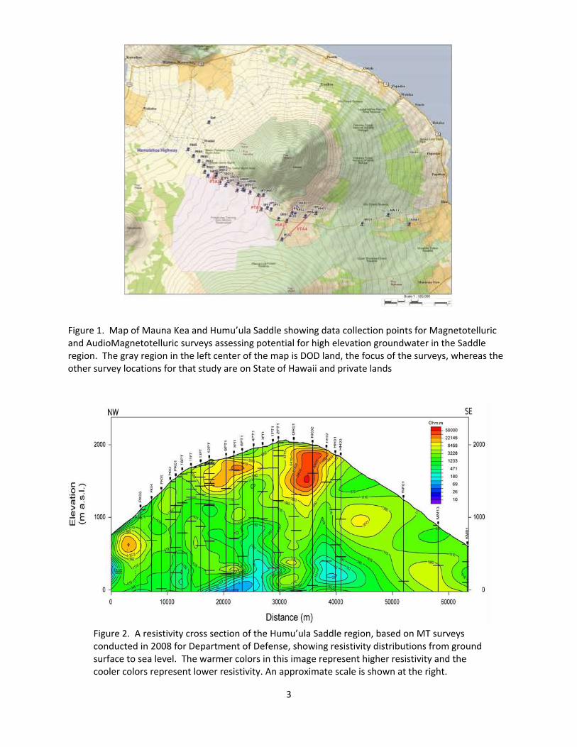
vicinity of Pohakuloa Training Area (Figure 1; Pierce and Thomas, 2008).
Overall, those survey results showed (Figure 2) shallow rocks as being highly resistive within the
center of the Saddle region, but deeper rocks having resistivities in the range of 1000 ohm-
meters to as low as 5 to 10 ohm-meters near sea level. We postulated groundwater saturation
3
Figure 1. Map of Mauna Kea and Humu’ula Saddle showing data collection points for Magnetotelluric and AudioMagnetotelluric surveys assessing potential for high elevation groundwater in the Saddle region. The gray region in the left center of the map is DOD land, the focus of the surveys, whereas the other survey locations for that study are on State of Hawaii and private lands
Figure 2. A resistivity cross section of the Humu’ula Saddle region, based on MT surveys conducted in 2008 for Department of Defense, showing resistivity distributions from ground surface to sea level. The warmer colors in this image represent higher resistivity and the cooler colors represent lower resistivity. An approximate scale is shown at the right.
4
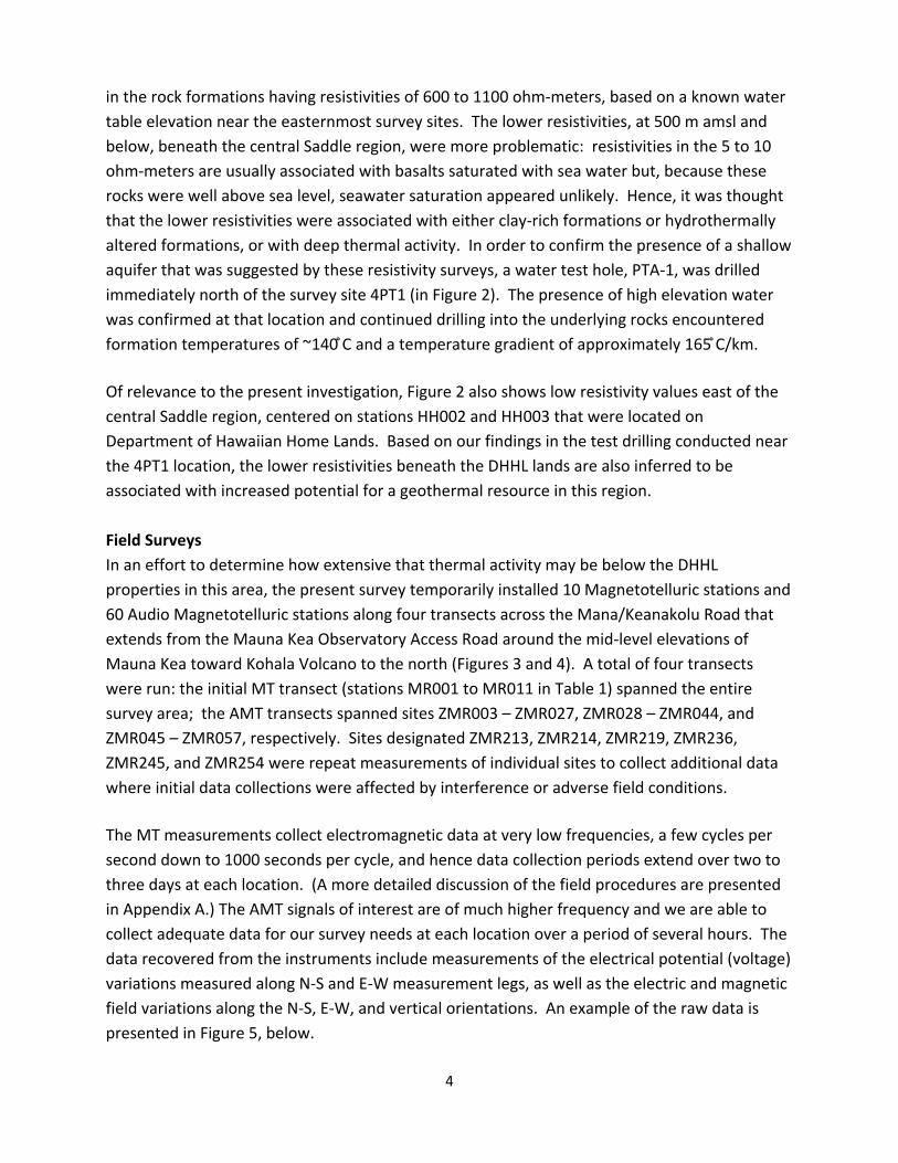
in the rock formations having resistivities of 600 to 1100 ohm-meters, based on a known water
table elevation near the easternmost survey sites. The lower resistivities, at 500 m amsl and
below, beneath the central Saddle region, were more problematic: resistivities in the 5 to 10
ohm-meters are usually associated with basalts saturated with sea water but, because these
rocks were well above sea level, seawater saturation appeared unlikely. Hence, it was thought
that the lower resistivities were associated with either clay-rich formations or hydrothermally
altered formations, or with deep thermal activity. In order to confirm the presence of a shallow
aquifer that was suggested by these resistivity surveys, a water test hole, PTA-1, was drilled
immediately north of the survey site 4PT1 (in Figure 2). The presence of high elevation water
was confirmed at that location and continued drilling into the underlying rocks encountered
formation temperatures of ~140 ̊C and a temperature gradient of approximately 165 ̊C/km.
Of relevance to the present investigation, Figure 2 also shows low resistivity values east of the
central Saddle region, centered on stations HH002 and HH003 that were located on
Department of Hawaiian Home Lands. Based on our findings in the test drilling conducted near
the 4PT1 location, the lower resistivities beneath the DHHL lands are also inferred to be
associated with increased potential for a geothermal resource in this region.
Field Surveys
In an effort to determine how extensive that thermal activity may be below the DHHL
properties in this area, the present survey temporarily installed 10 Magnetotelluric stations and
60 Audio Magnetotelluric stations along four transects across the Mana/Keanakolu Road that
extends from the Mauna Kea Observatory Access Road around the mid-level elevations of
Mauna Kea toward Kohala Volcano to the north (Figures 3 and 4). A total of four transects
were run: the initial MT transect (stations MR001 to MR011 in Table 1) spanned the entire
survey area; the AMT transects spanned sites ZMR003 – ZMR027, ZMR028 – ZMR044, and
ZMR045 – ZMR057, respectively. Sites designated ZMR213, ZMR214, ZMR219, ZMR236,
ZMR245, and ZMR254 were repeat measurements of individual sites to collect additional data
where initial data collections were affected by interference or adverse field conditions.
The MT measurements collect electromagnetic data at very low frequencies, a few cycles per
second down to 1000 seconds per cycle, and hence data collection periods extend over two to
three days at each location. (A more detailed discussion of the field procedures are presented
in Appendix A.) The AMT signals of interest are of much higher frequency and we are able to
collect adequate data for our survey needs at each location over a period of several hours. The
data recovered from the instruments include measurements of the electrical potential (voltage)
variations measured along N-S and E-W measurement legs, as well as the electric and magnetic
field variations along the N-S, E-W, and vertical orientations. An example of the raw data is
presented in Figure 5, below.

5
Figure 3. Satellite image, looking west, of the east flank of Mauna Kea showing the locations of the MT (designated MT 001 through MT 010) and AMT survey stations (designated ZMR001 through ZMR054). The MT stations are shown in green and the AMT stations shown in yellow and red. The stations shown in red correspond to a section of the survey that shows low resistivity values that may reflect evidence of current or past thermal activity within this region. A full page image is provided in Appendix A.
Data Analysis
The antenna coils that collect the electromagnetic signals are extraordinarily sensitive and can
receive interfering noise generated by lightening discharges occurring at distances of several
thousand kilometers, by variations in high tension power line currents at distances of several
tens of kilometers away, and even by electrical signals generated by large amplitude ocean
waves. Likewise, the electrical potential measurements can be affected by variations in the
ambient ground temperatures as well as environmental conditions like rainfall. Hence, the raw
data need to be intensively processed in order to filter out extraneous signals that are
irrelevant to our measurement objectives. After the data processing, we are able to compute
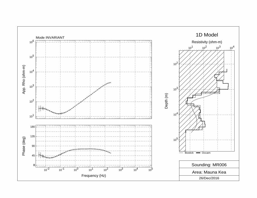
an apparent resistivity of the subsurface below that station as a function of frequency (Figure 6,
below). Error bars are shown on the apparent resistivity points where the error exceeds the
size of the data point; where no error bars are shown, the error of the value is less than the size
of the data point. Because the frequency of the electromagnetic signals affects the distance of
rock through which the signals can pass, the apparent resistivity as a function of frequency can
be converted to an apparent resistivity as a function of depth below the ground surface to yield
an apparent resistivity profile below each station (Figure 7, below). These apparent resistivity
curves show a modeled resistivity versus depth based on the data collected at each station.
The determination of the modeled resistivity with depth is done by an iterative process where
6
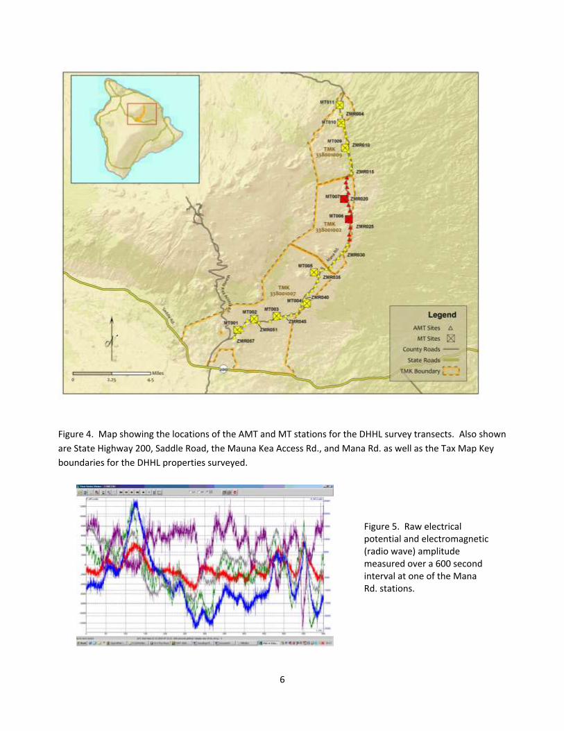
Figure 4. Map showing the locations of the AMT and MT stations for the DHHL survey transects. Also shown
are State Highway 200, Saddle Road, the Mauna Kea Access Rd., and Mana Rd. as well as the Tax Map Key
boundaries for the DHHL properties surveyed.
Figure 5. Raw electrical potential and electromagnetic (radio wave) amplitude measured over a 600 second interval at one of the Mana Rd. stations.
7
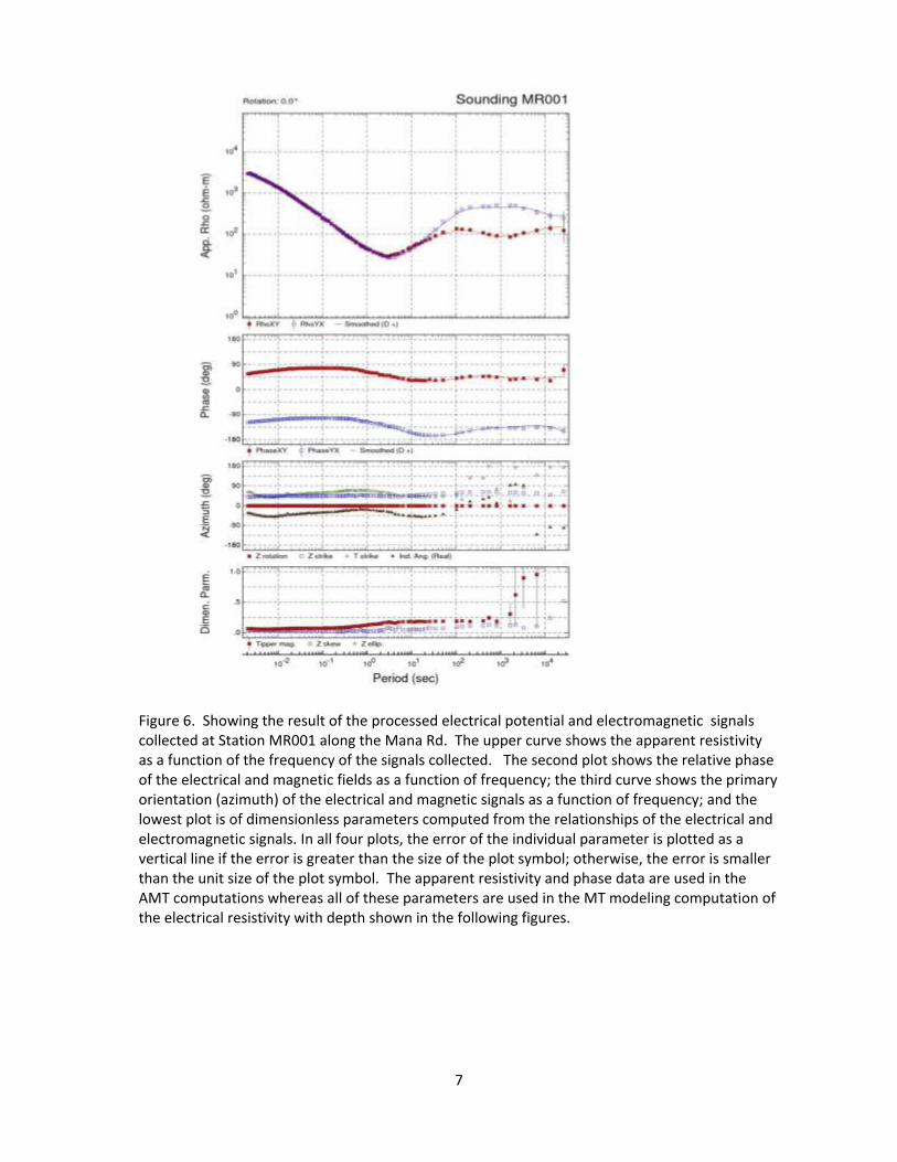
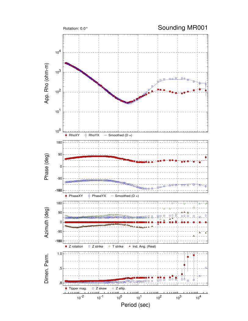
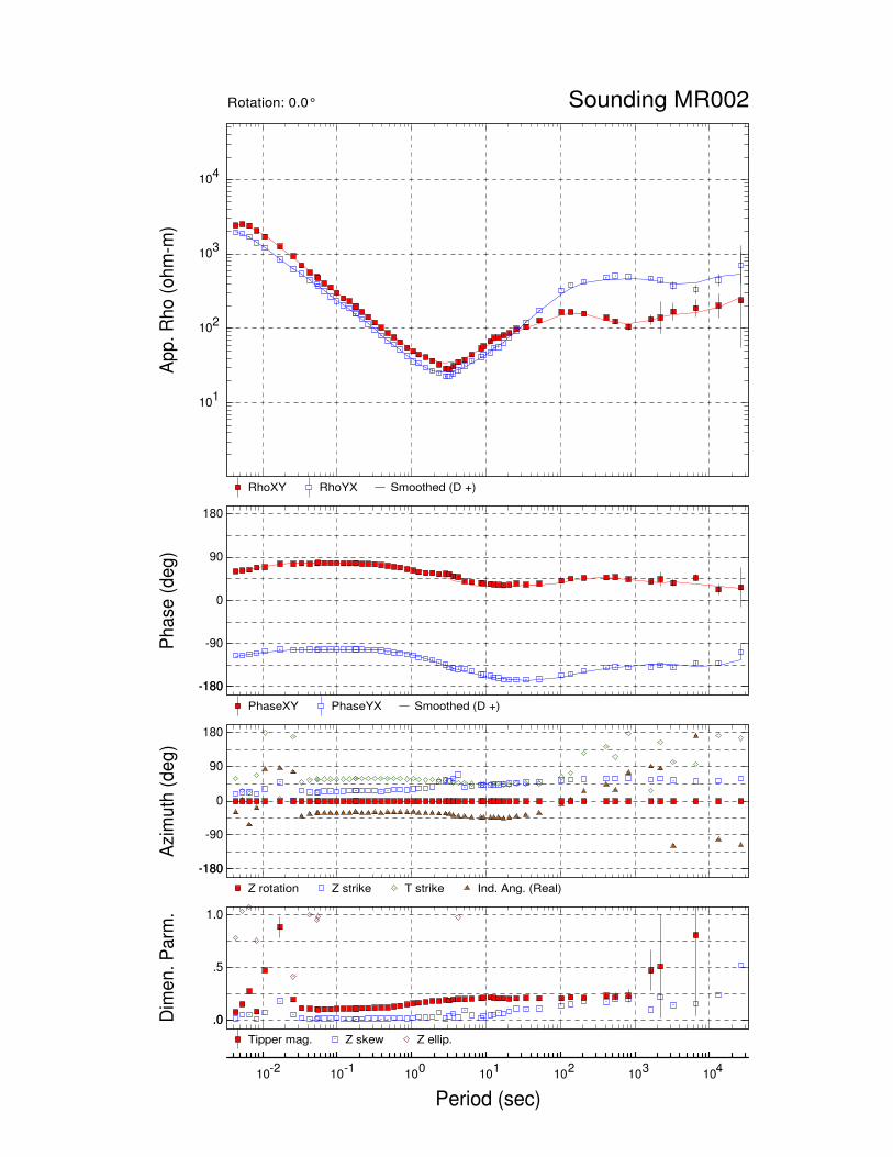
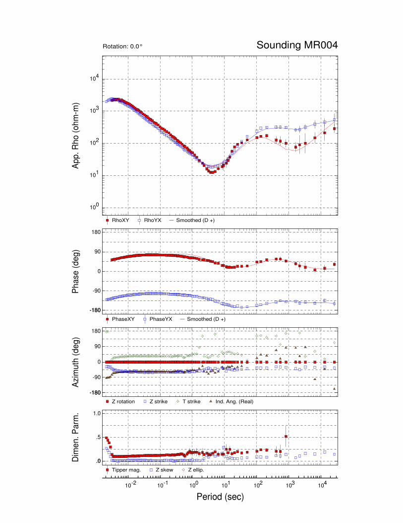
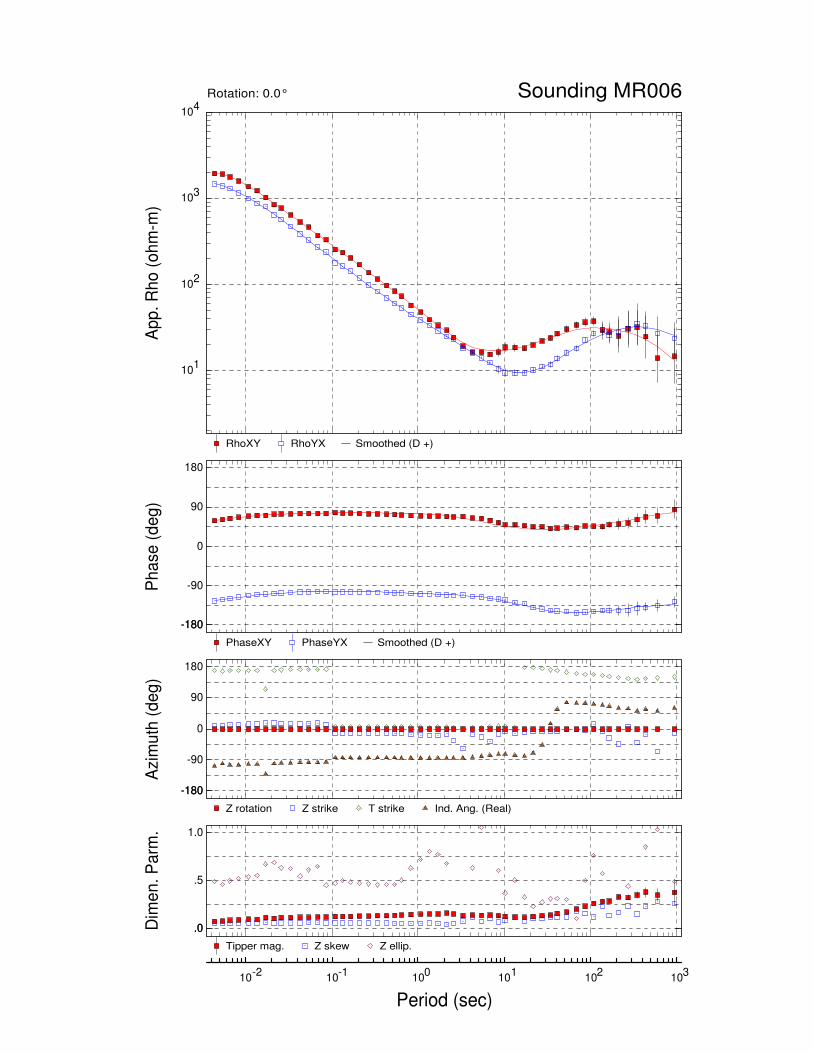
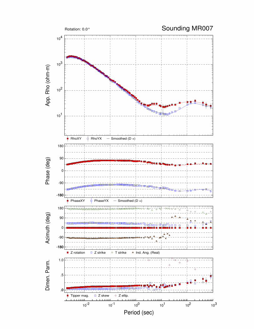
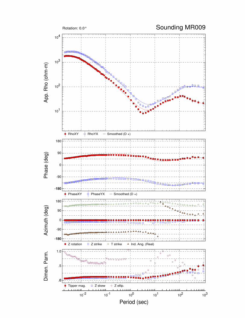
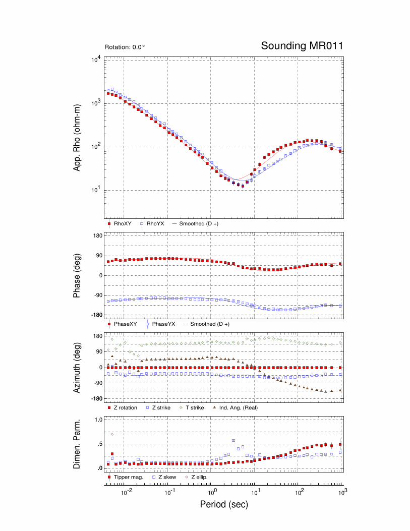
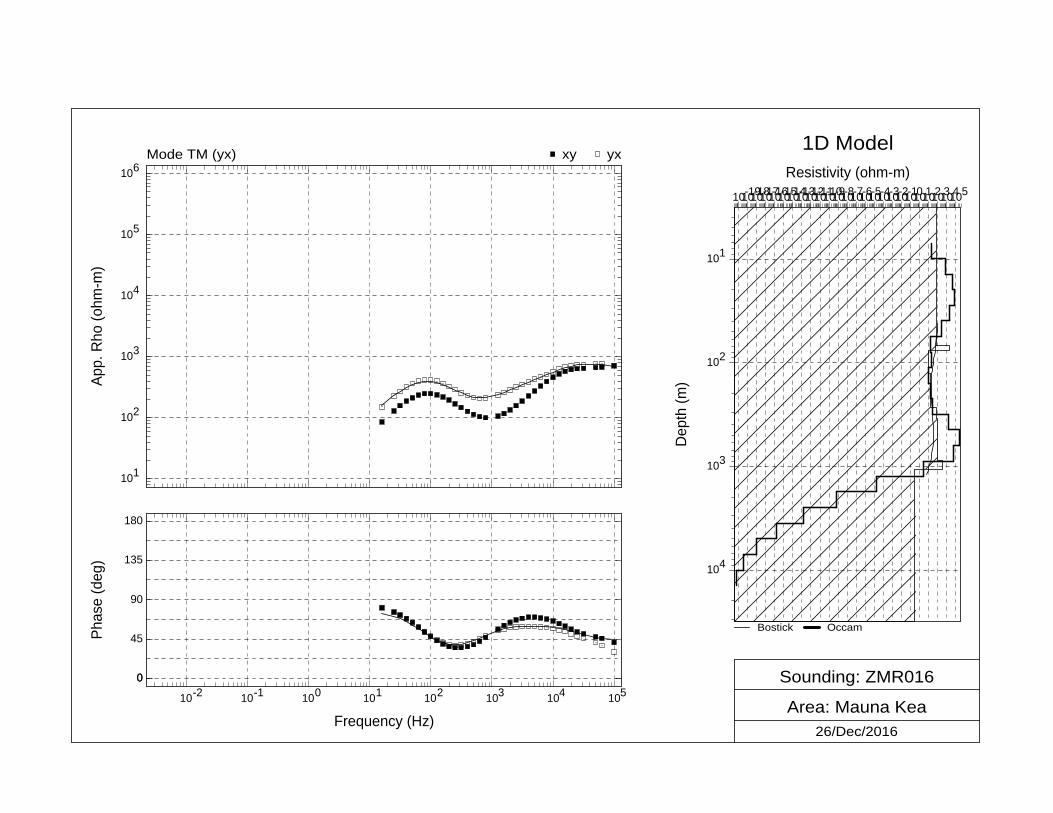
Figure 6. Showing the result of the processed electrical potential and electromagnetic signals collected at Station MR001 along the Mana Rd. The upper curve shows the apparent resistivity as a function of the frequency of the signals collected. The second plot shows the relative phase of the electrical and magnetic fields as a function of frequency; the third curve shows the primary orientation (azimuth) of the electrical and magnetic signals as a function of frequency; and the lowest plot is of dimensionless parameters computed from the relationships of the electrical and electromagnetic signals. In all four plots, the error of the individual parameter is plotted as a vertical line if the error is greater than the size of the plot symbol; otherwise, the error is smaller than the unit size of the plot symbol. The apparent resistivity and phase data are used in the AMT computations whereas all of these parameters are used in the MT modeling computation of the electrical resistivity with depth shown in the following figures.

8
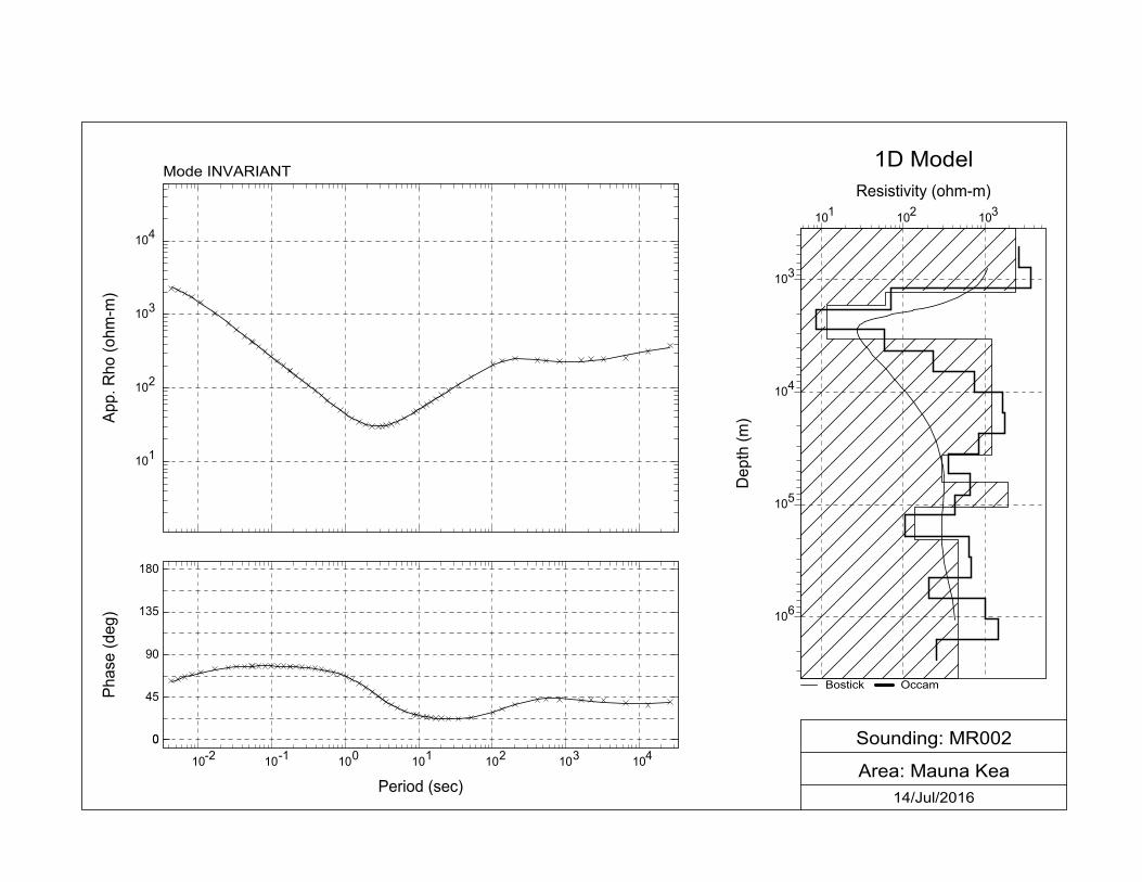
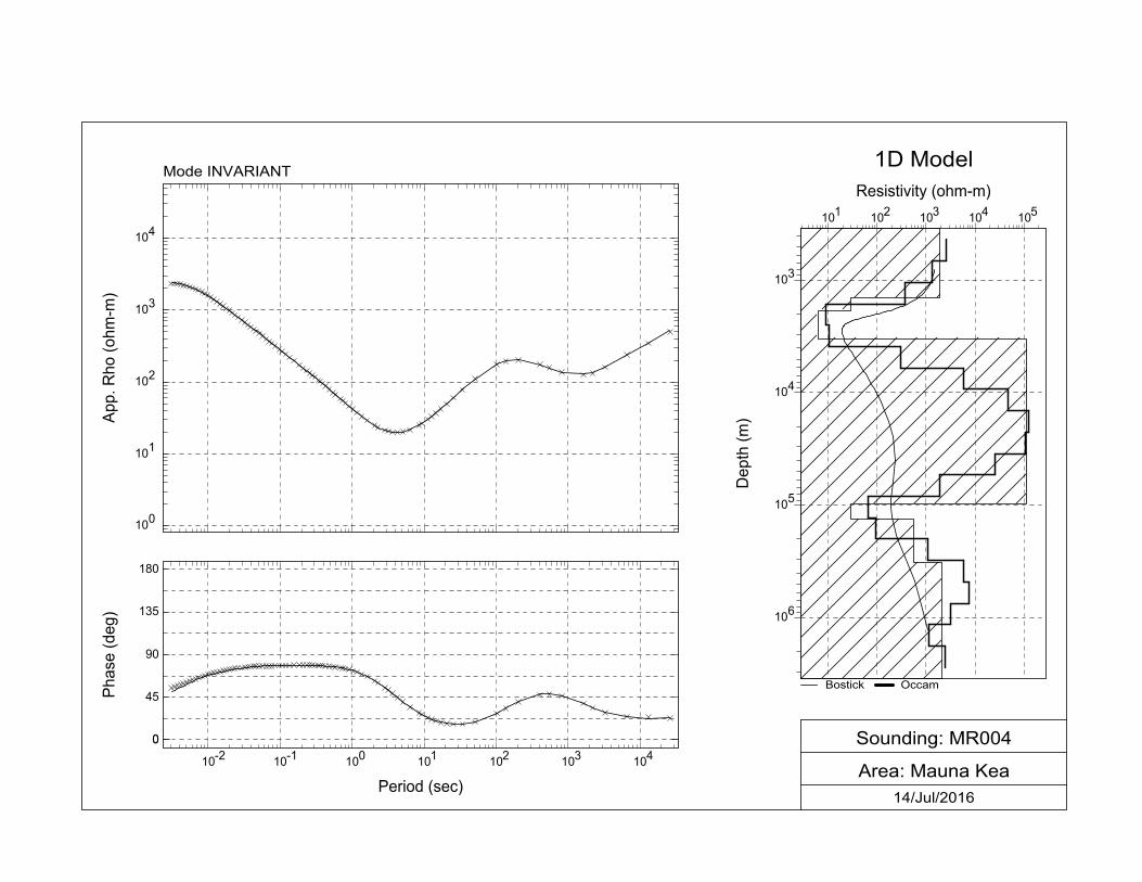
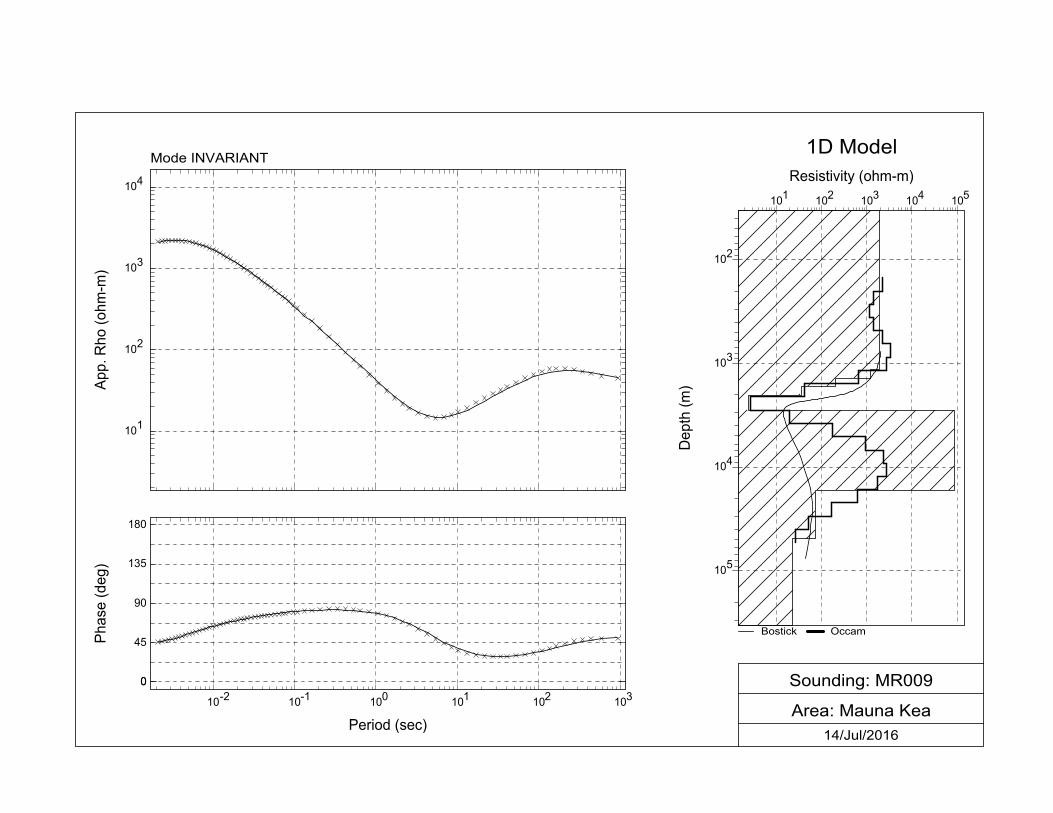
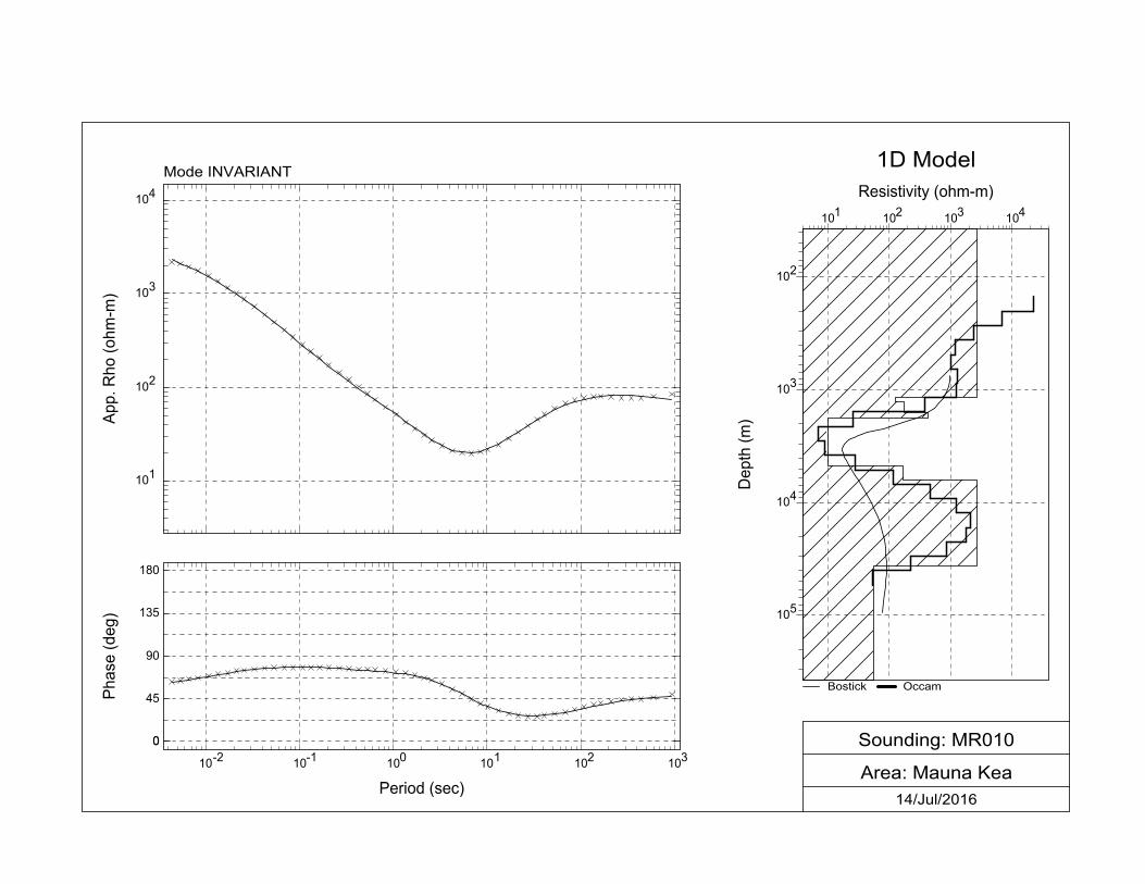
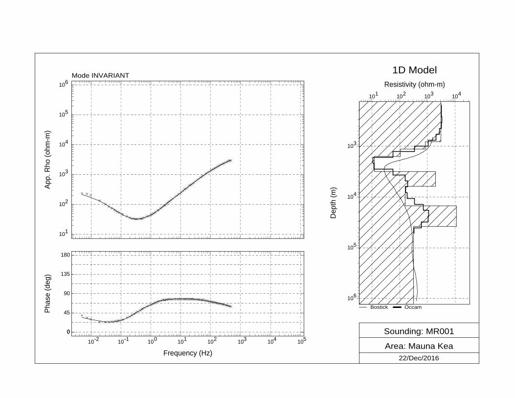
Figure 7. Presenting a 1-D model of the computed resistivity versus depth profile below MR001 measurement station. The graphics on the left show apparent resistivity verses the period of the signals processed (period is the inverse of frequency). The graphic on the right shows the computed resistivity versus depth, in meters, presented on a log scale (the uppermost division is 1000 m depth, the second division is 10,000 m depth).
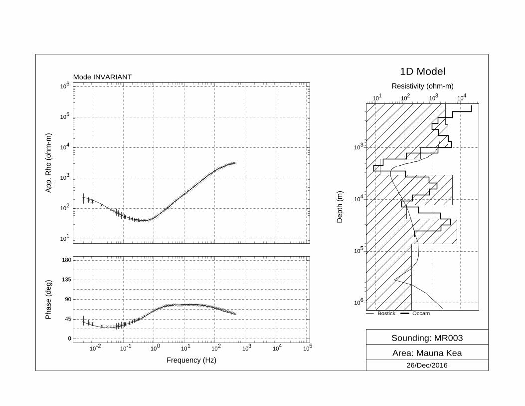
Figure 8. Presenting a 1-D model of the computed resistivity versus depth profile below MR005 measurement station. Comparing the modeled resistivity with depth between Station MR001 and MR005, it is apparent that the computed resistivity curves are quite different with the former showing a reduced resistivity at a shallower depth that remains low to depths much greater than those computed for Station MR001.

9
the resistivity and thickness of each layer is varied systematically to a point of model
convergence. Convergence is assumed when the difference between model run output varies
by less than 5%, or after 100 iterations of the model computation; where data are affected by
extraneous noise signals or other site conditions and 100 runs is unable to arrive at a 5% error,
model results with up to 10% error can be used, but larger modeled error outputs are discarded
from the survey sequence.
In the model output for station MR001, the resistivity is computed to be ~3000 ohm-meters
that declines to less than 2000 ohm-meters at a depth of approximately 700 m, and then to
about 300 ohm-meters at a depth of ~1000 m and then drops to about 20 ohm meters at a
depth of 1500 m, but then rises again at depths of 3000 m. Comparing the MR001 model with
that for Station MR005 (Figure 8), we see distinct differences in the computed resistivity profile:
the shallow resistivity is significantly lower, about 1000 ohm-meters, and remains low until a
depth of several hundred meters. It then rises over a narrow depth interval but falls off again
at 1000 m bgs and remains very low, ~10 ohm meters, from that depth to the total depth of
penetration of the signals collected. These results indicate that the computed resistivities deep
beneath Station MR005 are significantly lower than those below Station MR001 and hence have
a higher likelihood to be associated with a potential geothermal resource.
The 1-D models, when plotted together can give us a sense of how the resistivity with depth
varies along the Mana Road on the east flank of the island, but the computed resistivity for
each station relies on the data from that station alone. However, more sophisticated modeling
programs are able to, in effect, integrate the data collected at multiple stations in the sequence
of transects to yield a more accurate picture of the resistivity along the survey track. For this
type of analysis, we are using the WinGlink software package licensed from Schlumberger, one
of the large exploration and oil-service companies serving the energy and exploration
industries. That software allows us to integrate the MT and AMT measurements from multiple
stations to compute the resistivity distribution below (and adjacent to) the transects over the
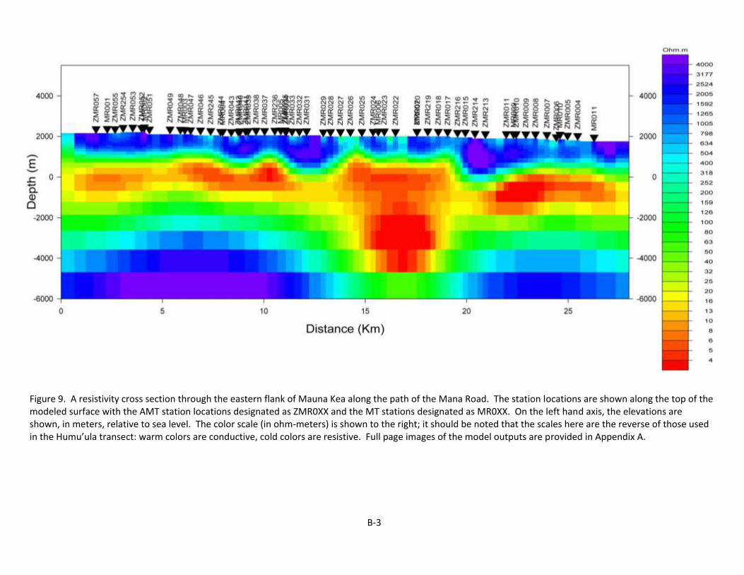
entire interval surveyed. That distribution is depicted in Figure 9, below (We note here that the
resistivity color scale produced with this software is reversed from that used in the Humu’ula
Saddle cross section: here warm colors are used to show conductive formations and cold colors
reflect higher resistivities). In that resistivity model we see that surface resistivities are
moderate to high (2500 to >4000 ohm-meters) down to depths of ~1000m but then begin to
fall off rapidly below that depth down to and somewhat below sea level, but then rise again at
increasing depth. The obvious exception to that broad trend is in the central region of the
survey: between stations ZMR027 and XMR016, there is a broad region of conductive material
that begins at somewhat higher elevations above sea level and extends to depths of about 5 km
10
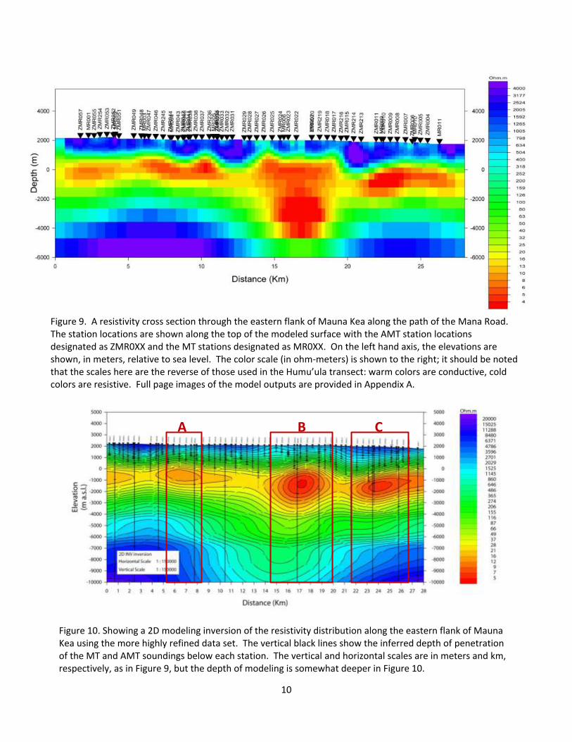
Figure 9. A resistivity cross section through the eastern flank of Mauna Kea along the path of the Mana Road. The station locations are shown along the top of the modeled surface with the AMT station locations designated as ZMR0XX and the MT stations designated as MR0XX. On the left hand axis, the elevations are shown, in meters, relative to sea level. The color scale (in ohm-meters) is shown to the right; it should be noted that the scales here are the reverse of those used in the Humu’ula transect: warm colors are conductive, cold colors are resistive. Full page images of the model outputs are provided in Appendix A.
Figure 10. Showing a 2D modeling inversion of the resistivity distribution along the eastern flank of Mauna Kea using the more highly refined data set. The vertical black lines show the inferred depth of penetration of the MT and AMT soundings below each station. The vertical and horizontal scales are in meters and km, respectively, as in Figure 9, but the depth of modeling is somewhat deeper in Figure 10.
A B C
11
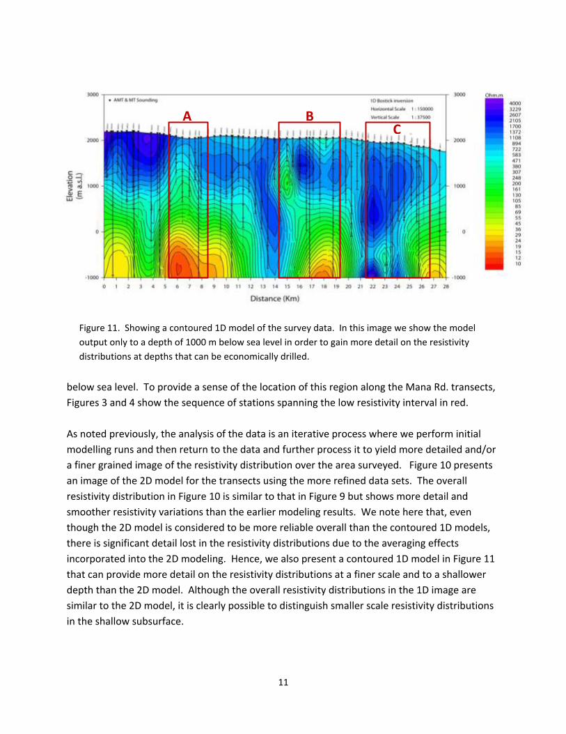
Figure 11. Showing a contoured 1D model of the survey data. In this image we show the model
output only to a depth of 1000 m below sea level in order to gain more detail on the resistivity
distributions at depths that can be economically drilled.
below sea level. To provide a sense of the location of this region along the Mana Rd. transects,
Figures 3 and 4 show the sequence of stations spanning the low resistivity interval in red.
As noted previously, the analysis of the data is an iterative process where we perform initial
modelling runs and then return to the data and further process it to yield more detailed and/or
a finer grained image of the resistivity distribution over the area surveyed. Figure 10 presents
an image of the 2D model for the transects using the more refined data sets. The overall
resistivity distribution in Figure 10 is similar to that in Figure 9 but shows more detail and
smoother resistivity variations than the earlier modeling results. We note here that, even
though the 2D model is considered to be more reliable overall than the contoured 1D models,
there is significant detail lost in the resistivity distributions due to the averaging effects
incorporated into the 2D modeling. Hence, we also present a contoured 1D model in Figure 11
that can provide more detail on the resistivity distributions at a finer scale and to a shallower
depth than the 2D model. Although the overall resistivity distributions in the 1D image are
similar to the 2D model, it is clearly possible to distinguish smaller scale resistivity distributions
in the shallow subsurface.
A C
B
12
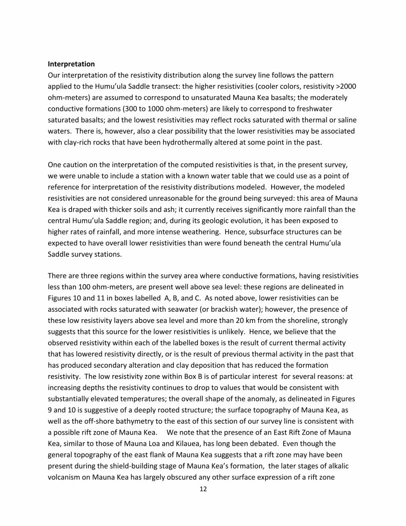
Interpretation
Our interpretation of the resistivity distribution along the survey line follows the pattern
applied to the Humu’ula Saddle transect: the higher resistivities (cooler colors, resistivity >2000
ohm-meters) are assumed to correspond to unsaturated Mauna Kea basalts; the moderately
conductive formations (300 to 1000 ohm-meters) are likely to correspond to freshwater
saturated basalts; and the lowest resistivities may reflect rocks saturated with thermal or saline
waters. There is, however, also a clear possibility that the lower resistivities may be associated
with clay-rich rocks that have been hydrothermally altered at some point in the past.
One caution on the interpretation of the computed resistivities is that, in the present survey,
we were unable to include a station with a known water table that we could use as a point of
reference for interpretation of the resistivity distributions modeled. However, the modeled
resistivities are not considered unreasonable for the ground being surveyed: this area of Mauna
Kea is draped with thicker soils and ash; it currently receives significantly more rainfall than the
central Humu’ula Saddle region; and, during its geologic evolution, it has been exposed to
higher rates of rainfall, and more intense weathering. Hence, subsurface structures can be
expected to have overall lower resistivities than were found beneath the central Humu’ula
Saddle survey stations.
There are three regions within the survey area where conductive formations, having resistivities
less than 100 ohm-meters, are present well above sea level: these regions are delineated in
Figures 10 and 11 in boxes labelled A, B, and C. As noted above, lower resistivities can be
associated with rocks saturated with seawater (or brackish water); however, the presence of
these low resistivity layers above sea level and more than 20 km from the shoreline, strongly
suggests that this source for the lower resistivities is unlikely. Hence, we believe that the
observed resistivity within each of the labelled boxes is the result of current thermal activity
that has lowered resistivity directly, or is the result of previous thermal activity in the past that
has produced secondary alteration and clay deposition that has reduced the formation
resistivity. The low resistivity zone within Box B is of particular interest for several reasons: at
increasing depths the resistivity continues to drop to values that would be consistent with
substantially elevated temperatures; the overall shape of the anomaly, as delineated in Figures
9 and 10 is suggestive of a deeply rooted structure; the surface topography of Mauna Kea, as
well as the off-shore bathymetry to the east of this section of our survey line is consistent with
a possible rift zone of Mauna Kea. We note that the presence of an East Rift Zone of Mauna
Kea, similar to those of Mauna Loa and Kilauea, has long been debated. Even though the
general topography of the east flank of Mauna Kea suggests that a rift zone may have been
present during the shield-building stage of Mauna Kea’s formation, the later stages of alkalic
volcanism on Mauna Kea has largely obscured any other surface expression of a rift zone
13
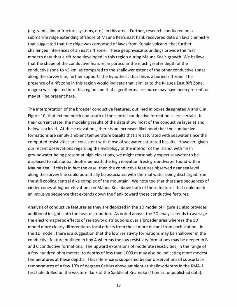
(e.g. vents, linear fracture systems, etc.) in this area. Further, research conducted on a
submarine ridge extending offshore of Mauna Kea’s east flank recovered data on lava chemistry
that suggested that the ridge was composed of lavas from Kohala volcano that further
challenged inferences of an east rift zone. These geophysical soundings provide the first
modern data that a rift zone developed in this region during Mauna Kea’s growth. We believe
that the shape of the conductive feature, in particular the much greater depth of the
conductive zone to >5 km, as compared to the shallower extent of the other conductive zones
along the survey line, further supports the hypothesis that this is a buried rift zone. The
presence of a rift zone in this region would indicate that, similar to the Kilauea East Rift Zone,
magma was injected into this region and that a geothermal resource may have been present, or
may still be present here.
The interpretation of the broader conductive features, outlined in boxes designated A and C in
Figure 10, that extend north and south of the central conductive formation is less certain. In
their current state, the modeling results of the data show most of the conductive layer at and
below sea level. At these elevations, there is an increased likelihood that the conductive
formations are simply ambient temperature basalts that are saturated with seawater since the
computed resistivities are consistent with those of seawater saturated basalts. However, given
our recent observations regarding the hydrology of the interior of the island, with fresh
groundwater being present at high elevations, we might reasonably expect seawater to be
displaced to substantial depths beneath the high elevation fresh groundwater found within
Mauna Kea. If this is in fact the case, then the conductive features observed near sea level
along the survey line could potentially be associated with thermal water being discharged from
the still cooling central dike complex of the mountain. We note too that there are sequences of
cinder cones at higher elevations on Mauna Kea above both of these features that could mark
an intrusive sequence that extends down the flank toward these conductive features.
Analysis of conductive features as they are depicted in the 1D model of Figure 11 also provides
additional insights into the heat distribution. As noted above, the 2D analysis tends to average
the electromagnetic effects of resistivity distributions over a broader area whereas the 1D
model more clearly differentiates local effects from those more distant from each station. In
the 1D model, there is a suggestion that the low resistivity formations may be shallower in the
conductive feature outlined in box A whereas the low resistivity formations may be deeper in B
and C conductive formations. The upward extensions of moderate resistivities, in the range of
a few hundred ohm meters, to depths of less than 1000 m may also be indicating more modest
temperatures at these depths. This inference is supported by our observations of subsurface
temperatures of a few 10’s of degrees Celsius above ambient at shallow depths in the KMA-1
test hole drilled on the western flank of the Saddle at Keamuku (Thomas, unpublished data).

14
Ancillary Note on Shallow Resistivity and Groundwater Potential
Although the primary purpose of the data collected during the current survey was to evaluate
the geothermal resource potential for this region, the data also provides insight into the
prospect of identifying high level groundwater resources along the survey line. Based on the
resistivity surveys conducted across the Humu’ula Saddle described above, we expect that
water saturated formations in this region to have resistivities in the range of a several hundred
to about 1000 ohm meters. Figure 11 identifies several areas along the survey line where
shallow resistivities fell within this range: in the interval of the survey designated by box A,
there is a “ridge” of conductive formation that extends quite close to the surface with
resistivities in the 300 to 700 ohm meter range; further north, between boxes A and B, there is
a pocket of resistivity that falls within the range of 700 to 900 ohm meters, and within box B are
formations ranging as low as 400 ohm meters. These shallow, low resistivity, formations would
have the highest potential for encountering a groundwater resource at shallow depths.
The nature of the aquifers here is, however, somewhat uncertain: the results of our exploratory
drilling work in the Saddle region demonstrated that both perched aquifers, of significant
thickness, as well as dike impounded aquifers were present within the central and western
Saddle region. With the higher rates of rainfall on the eastern flank of Mauna Kea, there is a
significant likelihood that both of these aquifer types would be present along the track
surveyed in the current study. Development of a water supply either by drilling, or by tunneling
along the top of perching formations (similar to water tunnels at Pahala in the Kau District),
could prove beneficial to the lessees of the Hawaiian Homes land surveyed.
Assessment of Resource Potential
The current modeling results of the MT and AMT data collected along the Mana Road transects
on the upper slope of Mauna Kea has provided us with inferred resistivity distributions that are
suggestive of as many as three geothermal prospects on the east flank of the mountain. The
lowest overall resistivity observed in the transect is within the central low-resistivity region
designed B; this lower resistivity can be interpreted to reflect the greatest likelihood of
encountering higher temperatures but the non-uniqueness of the resistivity-temperature
relationship, and the possibility of seawater intrusion into this deeper formation, would
nonetheless have to be considered. The association of this low-resistivity feature with an
inferred Mauna Kea East Rift Zone would suggest that a borehole into this section of the survey
transect would have the greatest potential for encountering a viable geothermal resource.
Our results are interpreted to indicate that the southern low-resistivity feature, designated A in
the above figures, would be the next most likely thermal source and the northern low-resistivity
feature would, based on the available data, be ranked the least likely to host a significant
resource.
15
A quantitative estimate of the probability for a thermal resource can be approximated, using
the methods of Ito, et al., (2016), but, because it would be based on the geophysical results
alone, that estimate would have a high degree of uncertainty. When comparing the observed
resistivities encountered in the Humu’ula Saddle survey (Pierce and Thomas, 2008) with those
observed in the current surveys, there is a likelihood of about 40% to 50% of encountering a
thermal resource in the lowest resistivity formations. The presence of an inferred rift zone
through this region would raise that probability to a somewhat higher value, but the absence of
data on shallow groundwater temperatures or chemistry in the area, as well as uncertainties
about the volume of the formation involved, would reduce our confidence in that value to 50%
or less.
It is not possible, using geophysics alone, to prove a viable geothermal resource; and the level
of confidence one can place in the results of a single geophysical survey line is lower still.
However, additional geophysical surveys could be performed that would increase the level of
confidence (or the converse) in making a decision to invest the necessary resources into a deep
exploration hole into any of these low-resistivity features. Our inference, based on the
resistivity distributions and topographic evidence, of a Mauna Kea East Rift Zone is less than
certain but additional resistivity surveys across the inferred strike of the postulated rift at lower
and higher elevations on the east flank of Mauna Kea could provide strong supporting evidence
of a substantial dike complex. Similarly, two or more gravity transects across the postulated rift
would allow us to make a somewhat more informed estimate of the intrusive mass associated
with the inferred rift zone and, from that, an approximate magnitude of the heat source
available. Both surveys, if they provide encouraging results with respect to resistivity
distributions and substantial intrusive volumes in that structure, would offer a higher level of
confidence that a significant and potentially viable thermal resource is associated with the
identified resistivity anomaly and that more expensive exploration options were justified.
Acknowledgements
A number of individuals have contributed to the work performed under this project. They
include:
Dr. Erin Wallin, a Post Doctoral trainee, who managed the field program and performed the
initial data validation;
Dr. Barry Lienert, who developed software for the processing and smoothing of the raw data
signals;
Dr. Graham Hill, who performed the initial data processing and modeling under this project;
Mr. Herb Pierce, who conducted the final data refinement and modeling of the data;
Ms. Georgianna Zelenak, who assisted with the field program and data validation; and
16
Mr. Ikaika Villanueva and Mr. Damian Aguier who conducted the field installations of the survey
stations and recorded field data.
References
Ito, G., N. Frazer, N. Lautze, D. Thomas, N. Hinz, D. Waller, R. Whittier, E. Wallin, 2016, Play
fairway analysis of geothermal resources across the state of Hawaii: 2. Resource probability
mapping, Geothermics, in press.
Pierce, H.A. and D.M. Thomas, 2009, Magnetotelluric and Audiomagnetotelluric Groundwater
Survey Along the Humu’ula Portion of Saddle Road Near and Around the Pohakuloa Training
Area, Hawaii, USGS Open File Report 2009–1135, 160 p.
Zohdy, A.A.R, and D. B. Jackson, 1969, Application of Deep Electrical Soundings for
Groundwater Exploration in Hawaii. Geophysics, Vol. 34, No. 4, pp. 584-600.
17
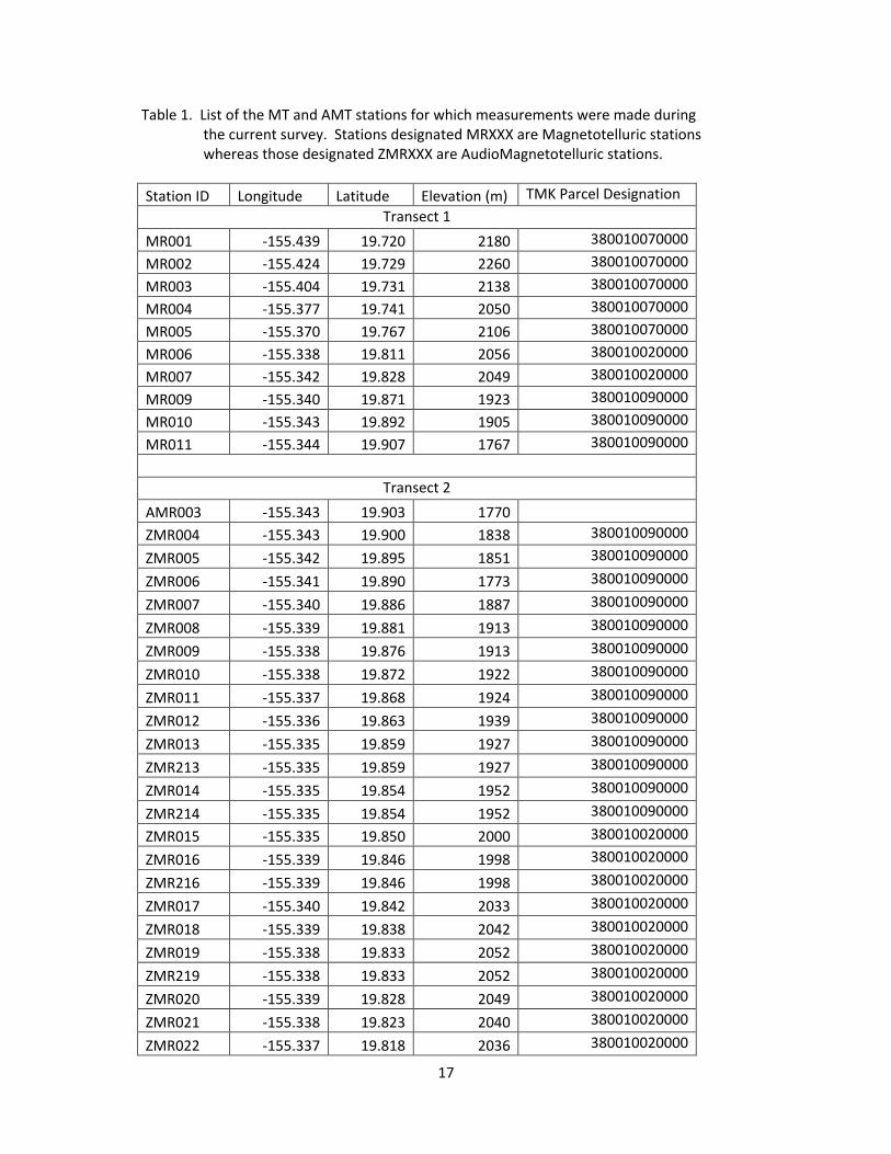
Table 1. List of the MT and AMT stations for which measurements were made during the current survey. Stations designated MRXXX are Magnetotelluric stations whereas those designated ZMRXXX are AudioMagnetotelluric stations.
Station ID Longitude Latitude Elevation (m) TMK Parcel Designation
Transect 1
MR001 -155.439 19.720 2180 380010070000
MR002 -155.424 19.729 2260 380010070000
MR003 -155.404 19.731 2138 380010070000
MR004 -155.377 19.741 2050 380010070000
MR005 -155.370 19.767 2106 380010070000
MR006 -155.338 19.811 2056 380010020000
MR007 -155.342 19.828 2049 380010020000
MR009 -155.340 19.871 1923 380010090000
MR010 -155.343 19.892 1905 380010090000
MR011 -155.344 19.907 1767 380010090000
Transect 2
AMR003 -155.343 19.903 1770
ZMR004 -155.343 19.900 1838 380010090000
ZMR005 -155.342 19.895 1851 380010090000
ZMR006 -155.341 19.890 1773 380010090000
ZMR007 -155.340 19.886 1887 380010090000
ZMR008 -155.339 19.881 1913 380010090000
ZMR009 -155.338 19.876 1913 380010090000
ZMR010 -155.338 19.872 1922 380010090000
ZMR011 -155.337 19.868 1924 380010090000
ZMR012 -155.336 19.863 1939 380010090000
ZMR013 -155.335 19.859 1927 380010090000
ZMR213 -155.335 19.859 1927 380010090000
ZMR014 -155.335 19.854 1952 380010090000
ZMR214 -155.335 19.854 1952 380010090000
ZMR015 -155.335 19.850 2000 380010020000
ZMR016 -155.339 19.846 1998 380010020000
ZMR216 -155.339 19.846 1998 380010020000
ZMR017 -155.340 19.842 2033 380010020000
ZMR018 -155.339 19.838 2042 380010020000
ZMR019 -155.338 19.833 2052 380010020000
ZMR219 -155.338 19.833 2052 380010020000
ZMR020 -155.339 19.828 2049 380010020000
ZMR021 -155.338 19.823 2040 380010020000
ZMR022 -155.337 19.818 2036 380010020000
18
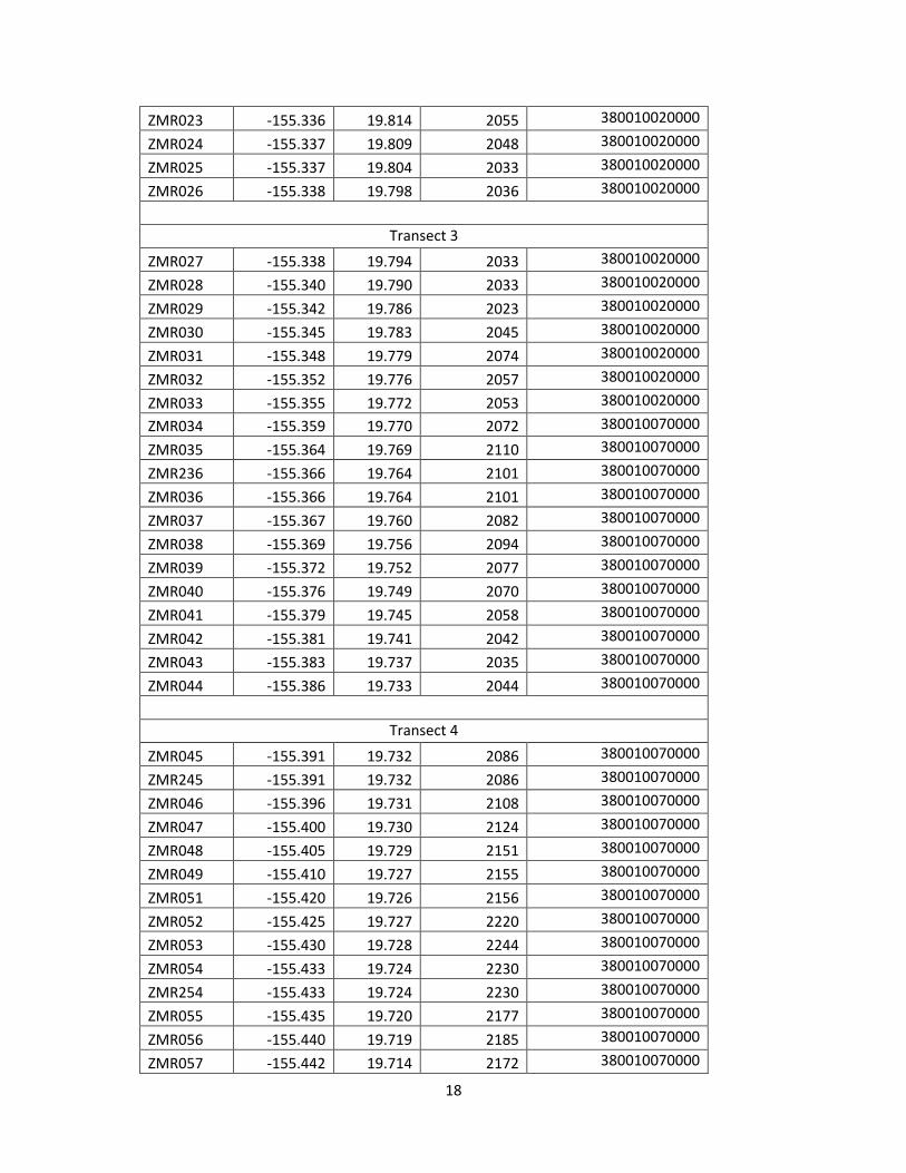
ZMR023 -155.336 19.814 2055 380010020000
ZMR024 -155.337 19.809 2048 380010020000
ZMR025 -155.337 19.804 2033 380010020000
ZMR026 -155.338 19.798 2036 380010020000
Transect 3
ZMR027 -155.338 19.794 2033 380010020000
ZMR028 -155.340 19.790 2033 380010020000
ZMR029 -155.342 19.786 2023 380010020000
ZMR030 -155.345 19.783 2045 380010020000
ZMR031 -155.348 19.779 2074 380010020000
ZMR032 -155.352 19.776 2057 380010020000
ZMR033 -155.355 19.772 2053 380010020000
ZMR034 -155.359 19.770 2072 380010070000
ZMR035 -155.364 19.769 2110 380010070000
ZMR236 -155.366 19.764 2101 380010070000
ZMR036 -155.366 19.764 2101 380010070000
ZMR037 -155.367 19.760 2082 380010070000
ZMR038 -155.369 19.756 2094 380010070000
ZMR039 -155.372 19.752 2077 380010070000
ZMR040 -155.376 19.749 2070 380010070000
ZMR041 -155.379 19.745 2058 380010070000
ZMR042 -155.381 19.741 2042 380010070000
ZMR043 -155.383 19.737 2035 380010070000
ZMR044 -155.386 19.733 2044 380010070000
Transect 4
ZMR045 -155.391 19.732 2086 380010070000
ZMR245 -155.391 19.732 2086 380010070000
ZMR046 -155.396 19.731 2108 380010070000
ZMR047 -155.400 19.730 2124 380010070000
ZMR048 -155.405 19.729 2151 380010070000
ZMR049 -155.410 19.727 2155 380010070000
ZMR051 -155.420 19.726 2156 380010070000
ZMR052 -155.425 19.727 2220 380010070000
ZMR053 -155.430 19.728 2244 380010070000
ZMR054 -155.433 19.724 2230 380010070000
ZMR254 -155.433 19.724 2230 380010070000
ZMR055 -155.435 19.720 2177 380010070000
ZMR056 -155.440 19.719 2185 380010070000
ZMR057 -155.442 19.714 2172 380010070000
A-1
Appendix A
The purpose of a Magnetotelluric and AudioMagnetotelluric Survey Program
These geophysical survey techniques will allow us to better map underground geologic
structures, water resources, and magmatic and hydrothermal systems. Current technology,
called magnetotelluric surveys (usually referred to as MT and AMT), allow us to map the
electrical conductivity of rocks at depths ranging from several hundred feet below the surface to
as much as 20,000 feet below the surface. Because the electrical conductivity of geologic
formations is the result of the type of rocks present, the presence (and salt content) of water in
the rocks, and the temperature of the rock, the method can identify groundwater aquifers,
distinguish between salt water and freshwater aquifers, and distinguish between different types
of rocks and can even be used to map underground pockets of magma. With appropriately
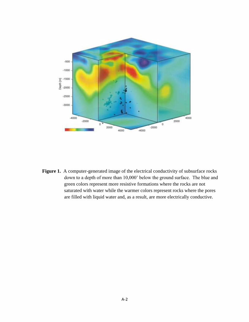
designed surveys, we can develop an image of the electrical conductivity similar to that shown in
Figure 1 below; the warmer colors represent highly conductive rocks whereas the cooler colors
represent more resistive rock formations. These surveys allow us to map the electrical resistivity
of the subsurface to depths of four to six kilometers below the ground surface. Areas of highly
resistive rocks (having resistivities more than several thousand ohm-meters) are likely to be
dense and dry rocks with neither water nor useable significant heat present; regions with
intermediate resistivity (several hundred to a few thousand ohm-meters) are likely to be less
dense rocks saturated with freshwater; and rocks with low resistivities (a few to a few tens of
ohm-meters) are likely to be rocks, at elevated temperatures, saturated with freshwater, or rocks
at ambient temperatures saturated with highly saline (sea) water.
A-2
Figure 1. A computer-generated image of the electrical conductivity of subsurface rocks
down to a depth of more than 10,000’ below the ground surface. The blue and
green colors represent more resistive formations where the rocks are not
saturated with water while the warmer colors represent rocks where the pores
are filled with liquid water and, as a result, are more electrically conductive.

A-3
Description of the field methods using
Magnetotelluric Surveys
Magnetotelluric surveys are considered a passive, non-invasive geophysical investigation. The
measurements are called passive because the instruments measure naturally occurring, very low
frequency, electromagnetic (EM) waves that penetrate into the earth. The instruments don’t
generate any EM signals or transmit any energy into the earth, they simply detect and record
variations in the electrical voltage and EM signals that continuously pass into and out of the
earth. The naturally occurring EM signals are similar to radio waves, but much lower power and
frequency. They induce the telluric currents that flow within the earth that this technique
measures. Analysis of the variations in the electric and magnetic signals enables us to determine
the electrical resistivity of the rocks and to identify groundwater flow occurring at varying depths
in the subsurface. Those measurements will also allow us to infer something about the types of
rocks that are present in the subsurface, the water present in those rocks (whether salt or fresh),
and their temperatures.
In order to perform a magnetotelluric survey, we use two (in some cases, three) antennas and
four specialized ground-contact electrodes with each connected to a data recording system. The
data system continuously records the voltage difference between the pairs of electrodes and
records the magnetic wave signals received by the antennas. The antennas consist of an iron rod
that is wrapped with many thousands of turns of fine copper wire, all encased in a fiberglass
tube. They are designed to collect incoming natural signals that, depending on their frequency,
penetrate to varying depths in the ground. The electrodes consist of a metal wire suspended in a
sodium chloride (table salt) solution contained in a plastic cup with a porous ceramic disk at the
bottom for electrical contact to the ground.
A photo of the antennas and electrodes, along with the recording box and the cables used is
shown in Figure 1. When placed at a field station, the equipment is laid out similar to that shown
in Figure 2. The electrodes and the antennas are laid out in a north-south and east-west
configuration with the electrodes being separated by a distance of 100 m to 200 m (330’ to 660’)
and the antennas separated by about 20 m (66’). A photo of a typical data collection station is
shown in Figure 3. The data acquisition unit is housed in a weatherproof box and is powered
with a conventional car battery. Once configured and data collection initiated, we would cover

A-4
the equipment with a tarp to further protect it from the weather and to reduce its visibility.
Figure 4 shows the shallow trench in which the antenna coil is buried; Figure 5 shows the
antenna after burial and ready to begin collecting data.
Figure 6 shows a typical electrode as it is placed in a shallow hole in the ground and prepared to
collect data; for our surveys, we will place the electrode in a fabric bag that has been partially
filled with hydrated bentonite clay to ensure good electrical contact with the ground. By using
the fabric bag, we will be able to recover all the clay from the hole leaving nothing behind at the
survey sites. Each of the electrodes and antenna coils are connected to the data collection box
using the wire cables shown in Figure 1. The need to bury the electrodes and antenna coils is
because of their extreme sensitivity; any type of vibration from wind or rain would produce
electrical “noise” that would interfere with the signals we are trying to record. In areas where
shallow trenching isn’t feasible or is not acceptable, we can weigh down the antennas with sand
bags to hold them in a stable configuration. Likewise, we will need to have the cables
connecting the electrodes and antennas to the data acquisition box held in a stable configuration,
and, in areas that are heavily vegetated, we may need to clear some vegetation to allow us to
weight the entire length of the cables to the ground with sand bags or soil.
We have four sets of instruments allowing us to install up to four stations at one time. We expect
to have each station in place for about three days to allow us to collect the data we need to
perform our analysis. As an example, the measurement stations will be spaced at distances of
1600’ to 3200’ apart over the geologic structure we are surveying. Depending on the size of the
area we are surveying, we may need to conduct measurements at as many as twenty to thirty
locations; this means that we would need to relocate all four stations, five to seven times, at
three-day intervals, in order to complete the survey. The field crew will restore each station site
to its original condition, by filling in the electrode holes and the antenna trenches, as they remove
the equipment.
The AudioMagnetotelluric stations are considerably less elaborate and require only a set of steel
stakes, driven into the ground by about 20 cm, and a data collection box and 12 volt battery. A
photo of a typical AMT station is shown in Figure 7.
A-5
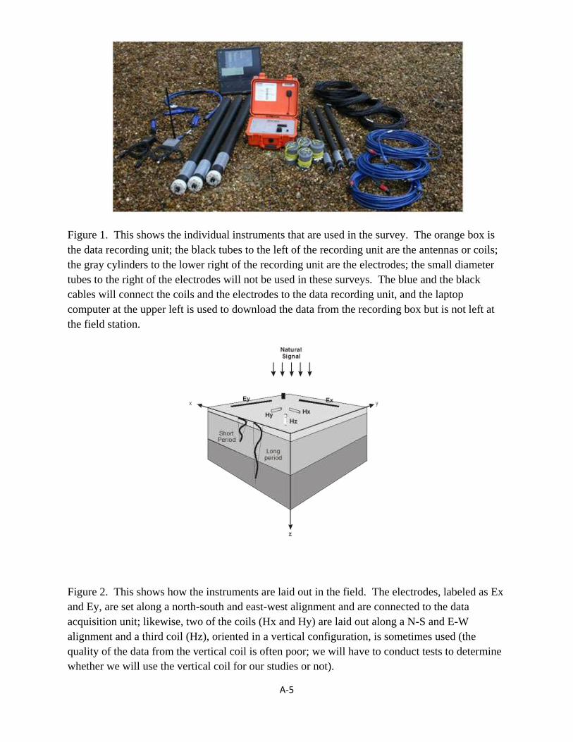
Figure 1. This shows the individual instruments that are used in the survey. The orange box is
the data recording unit; the black tubes to the left of the recording unit are the antennas or coils;
the gray cylinders to the lower right of the recording unit are the electrodes; the small diameter
tubes to the right of the electrodes will not be used in these surveys. The blue and the black
cables will connect the coils and the electrodes to the data recording unit, and the laptop
computer at the upper left is used to download the data from the recording box but is not left at
the field station.
Figure 2. This shows how the instruments are laid out in the field. The electrodes, labeled as Ex
and Ey, are set along a north-south and east-west alignment and are connected to the data
acquisition unit; likewise, two of the coils (Hx and Hy) are laid out along a N-S and E-W
alignment and a third coil (Hz), oriented in a vertical configuration, is sometimes used (the
quality of the data from the vertical coil is often poor; we will have to conduct tests to determine
whether we will use the vertical coil for our studies or not).

A-6
Figure 3. The data collection station
consists of the data recorder, housed
in a weatherproof box, along with a
standard car battery to provide power
for the recording system. We
typically cover the station with a tarp
to provide further protection from the
weather and to make the station less
visible.
Figure 4. Showing the shallow trench
used to bury the antenna coil.

A-7
Figure 5. The antenna coil
buried at the field site: once
the coil is aligned and leveled
in the trench, it is then covered
with soil from the trench to
stabilize it for the duration of
the data recording interval;
after the coil is recovered, we
refill the trench with its
original soil.
Figure 6. This is an image of
a typical installation of an
electrode for this type of
survey. The mud at the
bottom of the hole is a slurry
of soil and bentonite clay
that has been hydrated with
fresh water to allow for good
contact with the ground. For
our surveys, we will place
the electrode into a fabric
bag with hydrated bentonite
clay; the bag will be placed
in the hole with some water
and, at the end of the data
collection interval, we will
remove the bagged electrode
and all the bentonite clay and
refill the shallow hole with
its original soil.
A-8
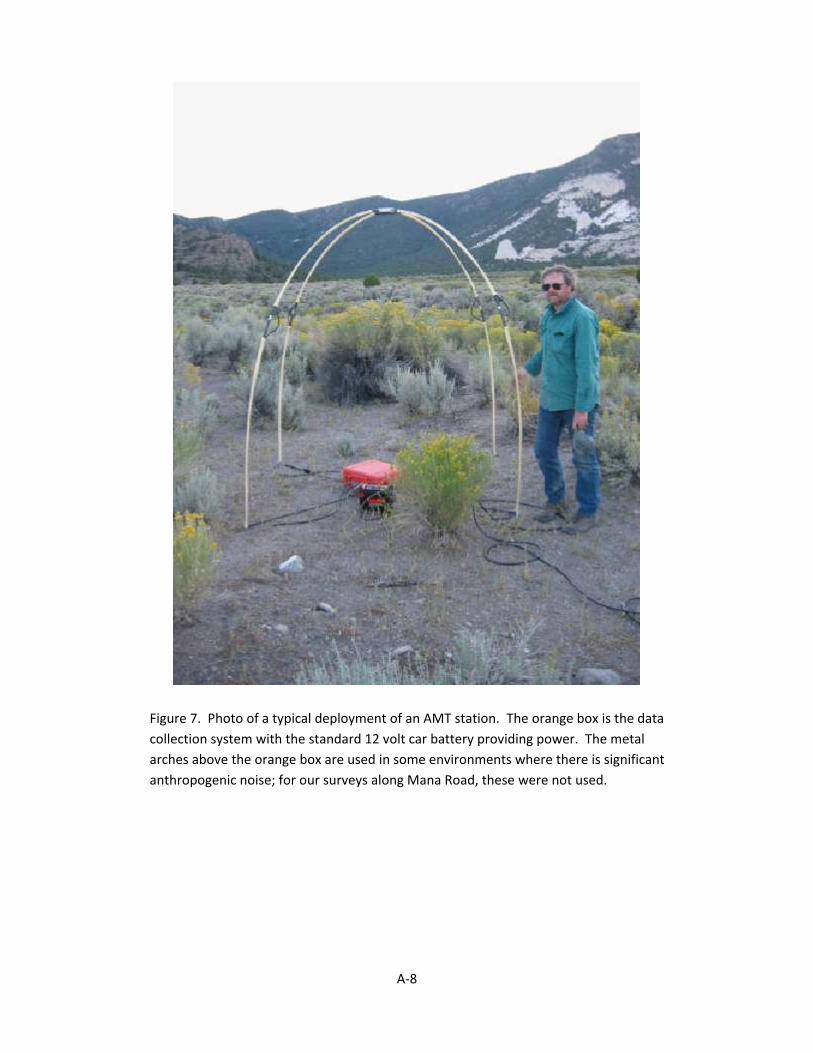
Figure 7. Photo of a typical deployment of an AMT station. The orange box is the data
collection system with the standard 12 volt car battery providing power. The metal
arches above the orange box are used in some environments where there is significant
anthropogenic noise; for our surveys along Mana Road, these were not used.

B-1
Appendix B
Full Page Images of Transect Station Locations and Model Outputs

B-2
Figure 3. Satellite image, looking west, of the east flank of Mauna Kea showing the locations of the MT (designated MT 001 through MT 010) and AMT survey stations (designated ZMR001 through ZMR054). The MT stations are shown in green and the AMT stations shown in yellow and red. The stations shown in red correspond to a section of the survey that shows low resistivity values that may reflect evidence of current or past thermal activity within this region.
B-3
Figure 9. A resistivity cross section through the eastern flank of Mauna Kea along the path of the Mana Road. The station locations are shown along the top of the modeled surface with the AMT station locations designated as ZMR0XX and the MT stations designated as MR0XX. On the left hand axis, the elevations are shown, in meters, relative to sea level. The color scale (in ohm-meters) is shown to the right; it should be noted that the scales here are the reverse of those used in the Humu’ula transect: warm colors are conductive, cold colors are resistive. Full page images of the model outputs are provided in Appendix A.

B-4
Figure 10. Showing a 2D modeling inversion of the resistivity distribution along the eastern flank of Mauna Kea using the more highly refined data set. The vertical black lines show the inferred depth of penetration of the MT and AMT soundings below each station. The vertical and horizontal scales are in meters and km, respectively, as in Figure 9, but the depth of modeling is somewhat deeper in Figure 10.

C-1
Appendix C
Plots of the Processed MT Data and 1D Apparent Resistivity Curves
104
103
102
101
100
Ap
p. R
ho
(o
hm
-m)
180
-180
90
0
-90
-180
Ph
ase
(d
eg
)
180
-180
90
0
-90
-180
Azim
uth
(d
eg
)
1.0
.0
.5
.0Dim
en
. P
arm
.
10-2
10-1
100
101
102
103
104
Period (sec)
RhoXY RhoYX Smoothed (D +)
PhaseXY PhaseYX Smoothed (D +)
Z rotation Z strike T strike Ind. Ang. (Real)
Tipper mag. Z skew Z ellip.
Sounding MR001Rotation: 0.0°

Sounding: MR001
Area: Mauna Kea
14/Jul/2016
Mode INVARIANT1D Model
Bostick Occam
104
103
102
101
100
Ap
p. R
ho
(o
hm
-m)
10-2
10-1
100
101
102
103
104
Period (sec)
180
0
135
90
45
0
Ph
ase
(d
eg
)
101
102
103
Resistivity (ohm-m)
103
104
105
106
De
pth
(m
)
104
103
102
101
Ap
p. R
ho
(o
hm
-m)
180
-180
90
0
-90
-180
Ph
ase
(d
eg
)
180
-180
90
0
-90
-180
Azim
uth
(d
eg
)
1.0
.0
.5
.0Dim
en
. P
arm
.
10-2
10-1
100
101
102
103
104
Period (sec)
RhoXY RhoYX Smoothed (D +)
PhaseXY PhaseYX Smoothed (D +)
Z rotation Z strike T strike Ind. Ang. (Real)
Tipper mag. Z skew Z ellip.
Sounding MR002Rotation: 0.0°
Sounding: MR002
Area: Mauna Kea
14/Jul/2016
Mode INVARIANT1D Model
Bostick Occam
104
103
102
101
Ap
p. R
ho
(o
hm
-m)
10-2
10-1
100
101
102
103
104
Period (sec)
180
0
135
90
45
0
Ph
ase
(d
eg
)
101
102
103
Resistivity (ohm-m)
103
104
105
106
De
pth
(m
)

104
103
102
101
Ap
p. R
ho
(o
hm
-m)
180
-180
90
0
-90
-180
Ph
ase
(d
eg
)
180
-180
90
0
-90
-180
Azim
uth
(d
eg
)
1.0
.0
.5
.0Dim
en
. P
arm
.
10-2
10-1
100
101
102
103
Period (sec)
RhoXY RhoYX Smoothed (D +)
PhaseXY PhaseYX Smoothed (D +)
Z rotation Z strike T strike Ind. Ang. (Real)
Tipper mag. Z skew Z ellip.
Sounding MR003Rotation: 0.0°

Sounding: MR003
Area: Mauna Kea
14/Jul/2016
Mode INVARIANT1D Model
Bostick Occam
104
103
102
101
Ap
p. R
ho
(o
hm
-m)
10-2
10-1
100
101
102
103
Period (sec)
180
0
135
90
45
0
Ph
ase
(d
eg
)
101
102
103
104
105
106
107
Resistivity (ohm-m)
103
104
105
106
De
pth
(m
)
104
103
102
101
100
Ap
p. R
ho
(o
hm
-m)
180
-180
90
0
-90
-180
Ph
ase
(d
eg
)
180
-180
90
0
-90
-180
Azim
uth
(d
eg
)
1.0
.0
.5
.0Dim
en
. P
arm
.
10-2
10-1
100
101
102
103
104
Period (sec)
RhoXY RhoYX Smoothed (D +)
PhaseXY PhaseYX Smoothed (D +)
Z rotation Z strike T strike Ind. Ang. (Real)
Tipper mag. Z skew Z ellip.
Sounding MR004Rotation: 0.0°
Sounding: MR004
Area: Mauna Kea
14/Jul/2016
Mode INVARIANT1D Model
Bostick Occam
104
103
102
101
100
Ap
p. R
ho
(o
hm
-m)
10-2
10-1
100
101
102
103
104
Period (sec)
180
0
135
90
45
0
Ph
ase
(d
eg
)
101
102
103
104
105
Resistivity (ohm-m)
103
104
105
106
De
pth
(m
)

103
102A
pp
. R
ho
(o
hm
-m)
180
-180
90
0
-90
-180
Ph
ase
(d
eg
)
180
-180
90
0
-90
-180
Azim
uth
(d
eg
)
1.0
.0
.5
.0Dim
en
. P
arm
.
10-2
10-1
100
Period (sec)
RhoXY RhoYX Smoothed (D +)
PhaseXY PhaseYX Smoothed (D +)
Z rotation Z strike T strike Ind. Ang. (Real)
Tipper mag. Z skew Z ellip.
Sounding MR005Rotation: 0.0°

Sounding: MR005
Area: Mauna Kea
14/Jul/2016
Mode INVARIANT1D Model
Bostick Occam
103
102A
pp
. R
ho
(o
hm
-m)
10-2
10-1
100
Period (sec)
180
0
135
90
45
0
Ph
ase
(d
eg
)
101
102
103
104
105
Resistivity (ohm-m)
102
103
104
105
De
pth
(m
)
104
103
102
101
Ap
p. R
ho
(o
hm
-m)
180
-180
90
0
-90
-180
Ph
ase
(d
eg
)
180
-180
90
0
-90
-180
Azim
uth
(d
eg
)
1.0
.0
.5
.0Dim
en
. P
arm
.
10-2
10-1
100
101
102
103
Period (sec)
RhoXY RhoYX Smoothed (D +)
PhaseXY PhaseYX Smoothed (D +)
Z rotation Z strike T strike Ind. Ang. (Real)
Tipper mag. Z skew Z ellip.
Sounding MR006Rotation: 0.0°

Sounding: MR006
Area: Mauna Kea
14/Jul/2016
Mode INVARIANT1D Model
Bostick Occam
104
103
102
101
Ap
p. R
ho
(o
hm
-m)
10-2
10-1
100
101
102
103
Period (sec)
180
0
135
90
45
0
Ph
ase
(d
eg
)
101
102
103
Resistivity (ohm-m)
102
103
104
105
De
pth
(m
)
104
103
102
101
Ap
p. R
ho
(o
hm
-m)
180
-180
90
0
-90
-180
Ph
ase
(d
eg
)
180
-180
90
0
-90
-180
Azim
uth
(d
eg
)
1.0
.0
.5
.0Dim
en
. P
arm
.
10-2
10-1
100
101
102
103
Period (sec)
RhoXY RhoYX Smoothed (D +)
PhaseXY PhaseYX Smoothed (D +)
Z rotation Z strike T strike Ind. Ang. (Real)
Tipper mag. Z skew Z ellip.
Sounding MR007Rotation: 0.0°

Sounding: MR007
Area: Mauna Kea
14/Jul/2016
Mode INVARIANT1D Model
Bostick Occam
104
103
102
101
Ap
p. R
ho
(o
hm
-m)
10-2
10-1
100
101
102
103
Period (sec)
180
0
135
90
45
0
Ph
ase
(d
eg
)
101
102
103
104
Resistivity (ohm-m)
102
103
104
105
De
pth
(m
)
104
103
102
101
Ap
p. R
ho
(o
hm
-m)
180
-180
90
0
-90
-180
Ph
ase
(d
eg
)
180
-180
90
0
-90
-180
Azim
uth
(d
eg
)
1.0
.0
.5
.0Dim
en
. P
arm
.
10-2
10-1
100
101
102
103
Period (sec)
RhoXY RhoYX Smoothed (D +)
PhaseXY PhaseYX Smoothed (D +)
Z rotation Z strike T strike Ind. Ang. (Real)
Tipper mag. Z skew Z ellip.
Sounding MR009Rotation: 0.0°
Sounding: MR009
Area: Mauna Kea
14/Jul/2016
Mode INVARIANT1D Model
Bostick Occam
104
103
102
101
Ap
p. R
ho
(o
hm
-m)
10-2
10-1
100
101
102
103
Period (sec)
180
0
135
90
45
0
Ph
ase
(d
eg
)
101
102
103
104
105
Resistivity (ohm-m)
102
103
104
105
De
pth
(m
)

104
103
102
101
Ap
p. R
ho
(o
hm
-m)
180
-180
90
0
-90
-180
Ph
ase
(d
eg
)
180
-180
90
0
-90
-180
Azim
uth
(d
eg
)
1.0
.0
.5
.0Dim
en
. P
arm
.
10-2
10-1
100
101
102
103
Period (sec)
RhoXY RhoYX Smoothed (D +)
PhaseXY PhaseYX Smoothed (D +)
Z rotation Z strike T strike Ind. Ang. (Real)
Tipper mag. Z skew Z ellip.
Sounding MR010Rotation: 0.0°
Sounding: MR010
Area: Mauna Kea
14/Jul/2016
Mode INVARIANT1D Model
Bostick Occam
104
103
102
101
Ap
p. R
ho
(o
hm
-m)
10-2
10-1
100
101
102
103
Period (sec)
180
0
135
90
45
0
Ph
ase
(d
eg
)
101
102
103
104
Resistivity (ohm-m)
102
103
104
105
De
pth
(m
)
104
103
102
101
Ap
p. R
ho
(o
hm
-m)
180
-180
90
0
-90
-180
Ph
ase
(d
eg
)
180
-180
90
0
-90
-180
Azim
uth
(d
eg
)
1.0
.0
.5
.0Dim
en
. P
arm
.
10-2
10-1
100
101
102
103
Period (sec)
RhoXY RhoYX Smoothed (D +)
PhaseXY PhaseYX Smoothed (D +)
Z rotation Z strike T strike Ind. Ang. (Real)
Tipper mag. Z skew Z ellip.
Sounding MR011Rotation: 0.0°

Sounding: MR011
Area: Mauna Kea
14/Jul/2016
Mode INVARIANT1D Model
Bostick Occam
104
103
102
101
Ap
p. R
ho
(o
hm
-m)
10-2
10-1
100
101
102
103
Period (sec)
180
0
135
90
45
0
Ph
ase
(d
eg
)
101
102
103
104
105
Resistivity (ohm-m)
102
103
104
105
De
pth
(m
)
Sounding: MR001
Area: Mauna Kea22/Dec/2016
Mode INVARIANT1D Model
Bostick Occam
106
105
104
103
102
101
App.
Rho
(ohm
-m)
10-2 10-1 100 101 102 103 104 105
Frequency (Hz)
180
0
135
90
45
0
Phas
e (d
eg)
101 102 103 104Resistivity (ohm-m)
103
104
105
106
Dep
th (m
)

Sounding: MR002
Area: Mauna Kea26/Dec/2016
Mode INVARIANT1D Model
Bostick Occam
106
105
104
103
102
101
App.
Rho
(ohm
-m)
10-2 10-1 100 101 102 103 104 105
Frequency (Hz)
180
0
135
90
45
0
Phas
e (d
eg)
101 102 103Resistivity (ohm-m)
102
103
104
105
Dep
th (m
)
Sounding: MR003
Area: Mauna Kea26/Dec/2016
Mode INVARIANT1D Model
Bostick Occam
106
105
104
103
102
101
App.
Rho
(ohm
-m)
10-2 10-1 100 101 102 103 104 105
Frequency (Hz)
180
0
135
90
45
0
Phas
e (d
eg)
101 102 103 104Resistivity (ohm-m)
103
104
105
106
Dep
th (m
)

Sounding: MR004
Area: Mauna Kea26/Dec/2016
Mode INVARIANT1D Model
Bostick Occam
106
105
104
103
102
101
App.
Rho
(ohm
-m)
10-2 10-1 100 101 102 103 104 105
Frequency (Hz)
180
0
135
90
45
0
Phas
e (d
eg)
101 102 103 104 105 106Resistivity (ohm-m)
103
104
105
106
Dep
th (m
)

Sounding: MR005
Area: Mauna Kea22/Dec/2016
Mode INVARIANT1D Model
Bostick Occam
106
105
104
103
102
101
App.
Rho
(ohm
-m)
10-2 10-1 100 101 102 103 104 105
Frequency (Hz)
180
0
135
90
45
0
Phas
e (d
eg)
101 102 103 104 105Resistivity (ohm-m)
102
103
104
105
Dep
th (m
)
Sounding: MR006
Area: Mauna Kea26/Dec/2016
Mode INVARIANT1D Model
Bostick Occam
106
105
104
103
102
101
App.
Rho
(ohm
-m)
10-2 10-1 100 101 102 103 104 105
Frequency (Hz)
180
0
135
90
45
0
Phas
e (d
eg)
101 102 103 104Resistivity (ohm-m)
102
103
104
105
Dep
th (m
)

Sounding: MR007
Area: Mauna Kea26/Dec/2016
Mode INVARIANT1D Model
Bostick Occam
106
105
104
103
102
101
App.
Rho
(ohm
-m)
10-2 10-1 100 101 102 103 104 105
Frequency (Hz)
180
0
135
90
45
0
Phas
e (d
eg)
101 102 103 104Resistivity (ohm-m)
102
103
104
105
Dep
th (m
)
Sounding: MR009
Area: Mauna Kea26/Dec/2016
Mode INVARIANT1D Model
Bostick Occam
106
105
104
103
102
101
App.
Rho
(ohm
-m)
10-2 10-1 100 101 102 103 104 105
Frequency (Hz)
180
0
135
90
45
0
Phas
e (d
eg)
101 102 103 104 105Resistivity (ohm-m)
102
103
104
105
Dep
th (m
)
Sounding: MR010
Area: Mauna Kea26/Dec/2016
Mode INVARIANT1D Model
Bostick Occam
106
105
104
103
102
101
App.
Rho
(ohm
-m)
10-2 10-1 100 101 102 103 104 105
Frequency (Hz)
180
0
135
90
45
0
Phas
e (d
eg)
101 102 103 104 105Resistivity (ohm-m)
102
103
104
105
Dep
th (m
)
Sounding: MR011
Area: Mauna Kea26/Dec/2016
Mode INVARIANT1D Model
Bostick Occam
106
105
104
103
102
101
App.
Rho
(ohm
-m)
10-2 10-1 100 101 102 103 104 105
Frequency (Hz)
180
0
135
90
45
0
Phas
e (d
eg)
101 102 103 104 105 106Resistivity (ohm-m)
102
103
104
105
Dep
th (m
)
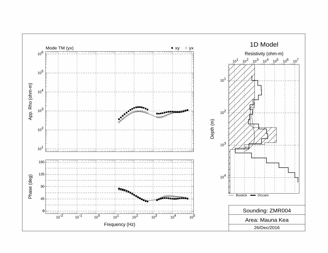
Sounding: ZMR004
Area: Mauna Kea26/Dec/2016
Mode TM (yx) yxxy1D Model
Bostick Occam
106
105
104
103
102
101
App.
Rho
(ohm
-m)
10-2 10-1 100 101 102 103 104 105
Frequency (Hz)
180
0
135
90
45
0
Phas
e (d
eg)
101 102 103 104 105 106 107Resistivity (ohm-m)
101
102
103
104
Dep
th (m
)

Sounding: ZMR005
Area: Mauna Kea26/Dec/2016
Mode TM (yx) yxxy1D Model
Bostick Occam
106
105
104
103
102
101
App.
Rho
(ohm
-m)
10-2 10-1 100 101 102 103 104 105
Frequency (Hz)
180
0
135
90
45
0
Phas
e (d
eg)
101 102 103 104Resistivity (ohm-m)
101
102
103
104
Dep
th (m
)

Sounding: ZMR006
Area: Mauna Kea26/Dec/2016
Mode TM (yx) yxxy1D Model
Bostick Occam
106
105
104
103
102
101
App.
Rho
(ohm
-m)
10-2 10-1 100 101 102 103 104 105
Frequency (Hz)
180
0
135
90
45
0
Phas
e (d
eg)
10-410-310-210-1100 101 102 103 104 105Resistivity (ohm-m)
101
102
103
104
Dep
th (m
)

Sounding: ZMR007
Area: Mauna Kea26/Dec/2016
Mode TM (yx) yxxy1D Model
Bostick Occam
106
105
104
103
102
101
App.
Rho
(ohm
-m)
10-2 10-1 100 101 102 103 104 105
Frequency (Hz)
180
0
135
90
45
0
Phas
e (d
eg)
10-2 10-1 100 101 102 103 104Resistivity (ohm-m)
101
102
103
104
Dep
th (m
)

Sounding: ZMR008
Area: Mauna Kea26/Dec/2016
Mode TM (yx) yxxy1D Model
Bostick Occam
106
105
104
103
102
101
App.
Rho
(ohm
-m)
10-2 10-1 100 101 102 103 104 105
Frequency (Hz)
180
0
135
90
45
0
Phas
e (d
eg)
10-410-310-210-1100 101102 103 104 105 106Resistivity (ohm-m)
101
102
103
104
Dep
th (m
)

Sounding: ZMR009
Area: Mauna Kea26/Dec/2016
Mode TM (yx) yxxy1D Model
Bostick Occam
106
105
104
103
102
101
App.
Rho
(ohm
-m)
10-2 10-1 100 101 102 103 104 105
Frequency (Hz)
180
0
135
90
45
0
Phas
e (d
eg)
10-2 10-1 100 101 102 103 104 105 106Resistivity (ohm-m)
101
102
103
104
Dep
th (m
)

Sounding: ZMR010
Area: Mauna Kea26/Dec/2016
Mode TM (yx) yxxy1D Model
Bostick Occam
106
105
104
103
102
101
App.
Rho
(ohm
-m)
10-2 10-1 100 101 102 103 104 105
Frequency (Hz)
180
0
135
90
45
0
Phas
e (d
eg)
101 102 103 104 105Resistivity (ohm-m)
101
102
103
104
Dep
th (m
)
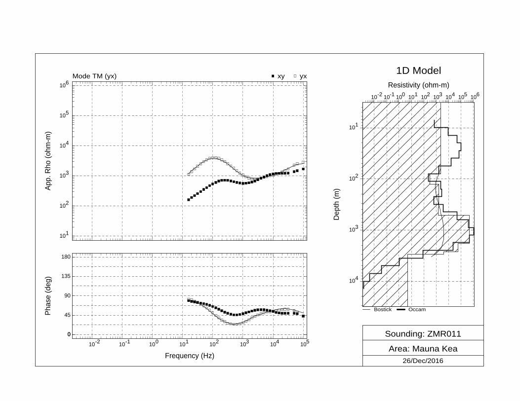
Sounding: ZMR011
Area: Mauna Kea26/Dec/2016
Mode TM (yx) yxxy1D Model
Bostick Occam
106
105
104
103
102
101
App.
Rho
(ohm
-m)
10-2 10-1 100 101 102 103 104 105
Frequency (Hz)
180
0
135
90
45
0
Phas
e (d
eg)
10-2 10-1 100 101 102 103 104 105 106Resistivity (ohm-m)
101
102
103
104
Dep
th (m
)

Sounding: ZMR012
Area: Mauna Kea26/Dec/2016
Mode TM (yx) yxxy1D Model
Bostick Occam
106
105
104
103
102
101
App.
Rho
(ohm
-m)
10-2 10-1 100 101 102 103 104 105
Frequency (Hz)
180
0
135
90
45
0
Phas
e (d
eg)
10-410-310-210-1100 101 102 103 104 105Resistivity (ohm-m)
101
102
103
104
Dep
th (m
)
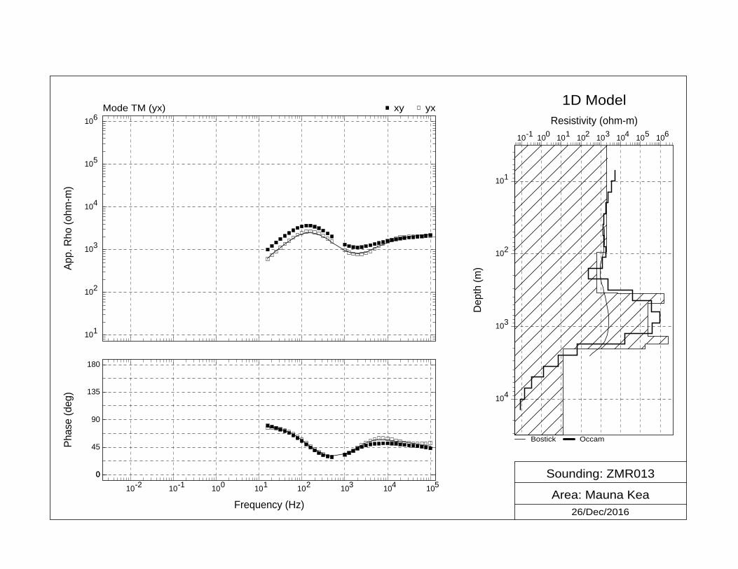
Sounding: ZMR013
Area: Mauna Kea26/Dec/2016
Mode TM (yx) yxxy1D Model
Bostick Occam
106
105
104
103
102
101
App.
Rho
(ohm
-m)
10-2 10-1 100 101 102 103 104 105
Frequency (Hz)
180
0
135
90
45
0
Phas
e (d
eg)
10-1 100 101 102 103 104 105 106Resistivity (ohm-m)
101
102
103
104
Dep
th (m
)
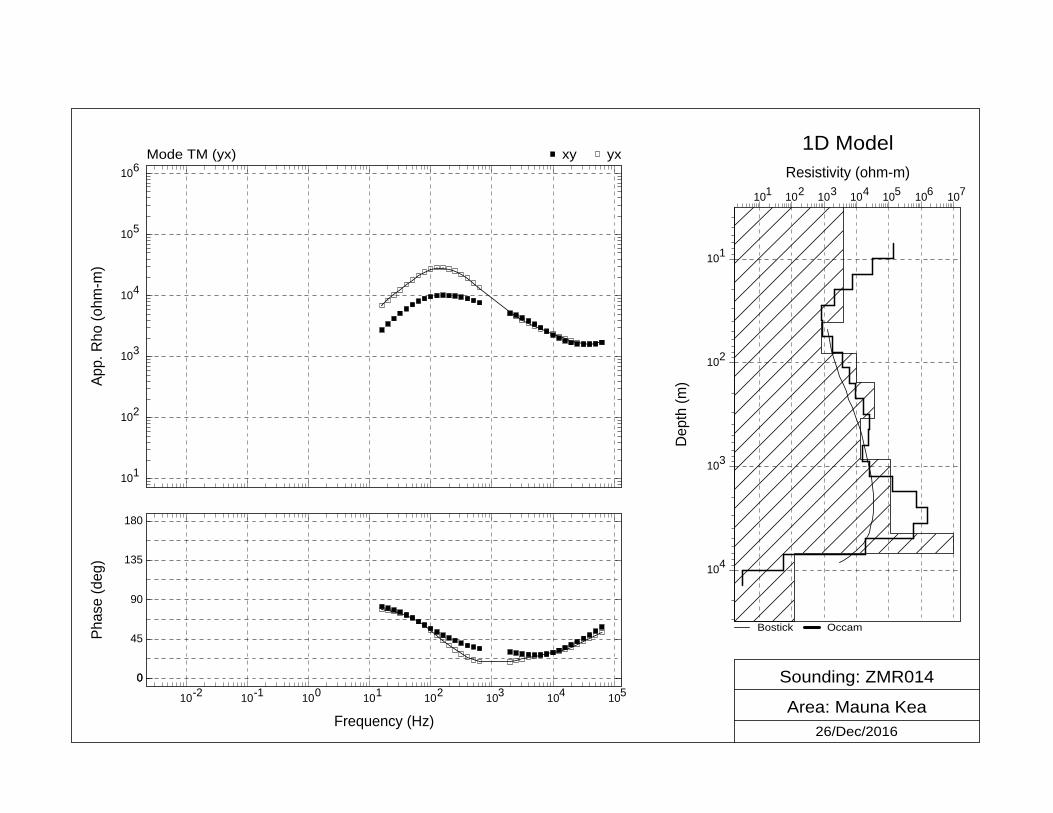
Sounding: ZMR014
Area: Mauna Kea26/Dec/2016
Mode TM (yx) yxxy1D Model
Bostick Occam
106
105
104
103
102
101
App.
Rho
(ohm
-m)
10-2 10-1 100 101 102 103 104 105
Frequency (Hz)
180
0
135
90
45
0
Phas
e (d
eg)
101 102 103 104 105 106 107Resistivity (ohm-m)
101
102
103
104
Dep
th (m
)

Sounding: ZMR015
Area: Mauna Kea26/Dec/2016
Mode TM (yx) yxxy1D Model
Bostick Occam
106
105
104
103
102
101
App.
Rho
(ohm
-m)
10-2 10-1 100 101 102 103 104 105
Frequency (Hz)
180
0
135
90
45
0
Phas
e (d
eg)
10-510-410-310-210-1100101102103104105106Resistivity (ohm-m)
101
102
103
104
Dep
th (m
)
Sounding: ZMR016
Area: Mauna Kea26/Dec/2016
Mode TM (yx) yxxy1D Model
Bostick Occam
106
105
104
103
102
101
App.
Rho
(ohm
-m)
10-2 10-1 100 101 102 103 104 105
Frequency (Hz)
180
0
135
90
45
0
Phas
e (d
eg)
10-1910-1810-1710-1610-1510-1410-1310-1210-1110-1010-910-810-710-610-510-410-310-210-1100101102103104105Resistivity (ohm-m)
101
102
103
104
Dep
th (m
)
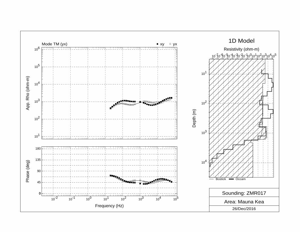
Sounding: ZMR017
Area: Mauna Kea26/Dec/2016
Mode TM (yx) yxxy1D Model
Bostick Occam
106
105
104
103
102
101
App.
Rho
(ohm
-m)
10-2 10-1 100 101 102 103 104 105
Frequency (Hz)
180
0
135
90
45
0
Phas
e (d
eg)
10-710-610-510-410-310-210-1100101102103104105Resistivity (ohm-m)
101
102
103
104
Dep
th (m
)
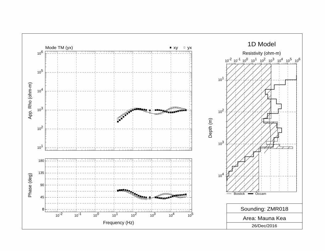
Sounding: ZMR018
Area: Mauna Kea26/Dec/2016
Mode TM (yx) yxxy1D Model
Bostick Occam
106
105
104
103
102
101
App.
Rho
(ohm
-m)
10-2 10-1 100 101 102 103 104 105
Frequency (Hz)
180
0
135
90
45
0
Phas
e (d
eg)
10-2 10-1 100 101 102 103 104 105 106Resistivity (ohm-m)
101
102
103
104
Dep
th (m
)
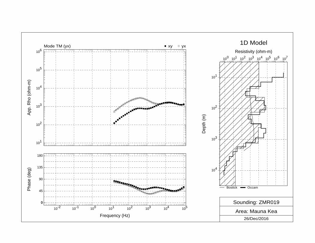
Sounding: ZMR019
Area: Mauna Kea26/Dec/2016
Mode TM (yx) yxxy1D Model
Bostick Occam
106
105
104
103
102
101
App.
Rho
(ohm
-m)
10-2 10-1 100 101 102 103 104 105
Frequency (Hz)
180
0
135
90
45
0
Phas
e (d
eg)
100 101 102 103 104 105 106 107Resistivity (ohm-m)
101
102
103
104
Dep
th (m
)

Sounding: ZMR020
Area: Mauna Kea26/Dec/2016
Mode TM (yx) yxxy1D Model
Bostick Occam
106
105
104
103
102
101
App.
Rho
(ohm
-m)
10-2 10-1 100 101 102 103 104 105
Frequency (Hz)
180
0
135
90
45
0
Phas
e (d
eg)
10-510-410-310-210-1100101102103104105106Resistivity (ohm-m)
101
102
103
104
Dep
th (m
)

Sounding: ZMR021
Area: Mauna Kea26/Dec/2016
Mode TM (yx) yxxy1D Model
Bostick Occam
106
105
104
103
102
101
App.
Rho
(ohm
-m)
10-2 10-1 100 101 102 103 104 105
Frequency (Hz)
180
0
135
90
45
0
Phas
e (d
eg)
100101102103104105106107108109101010111012101310141015Resistivity (ohm-m)
101
102
103
104
Dep
th (m
)
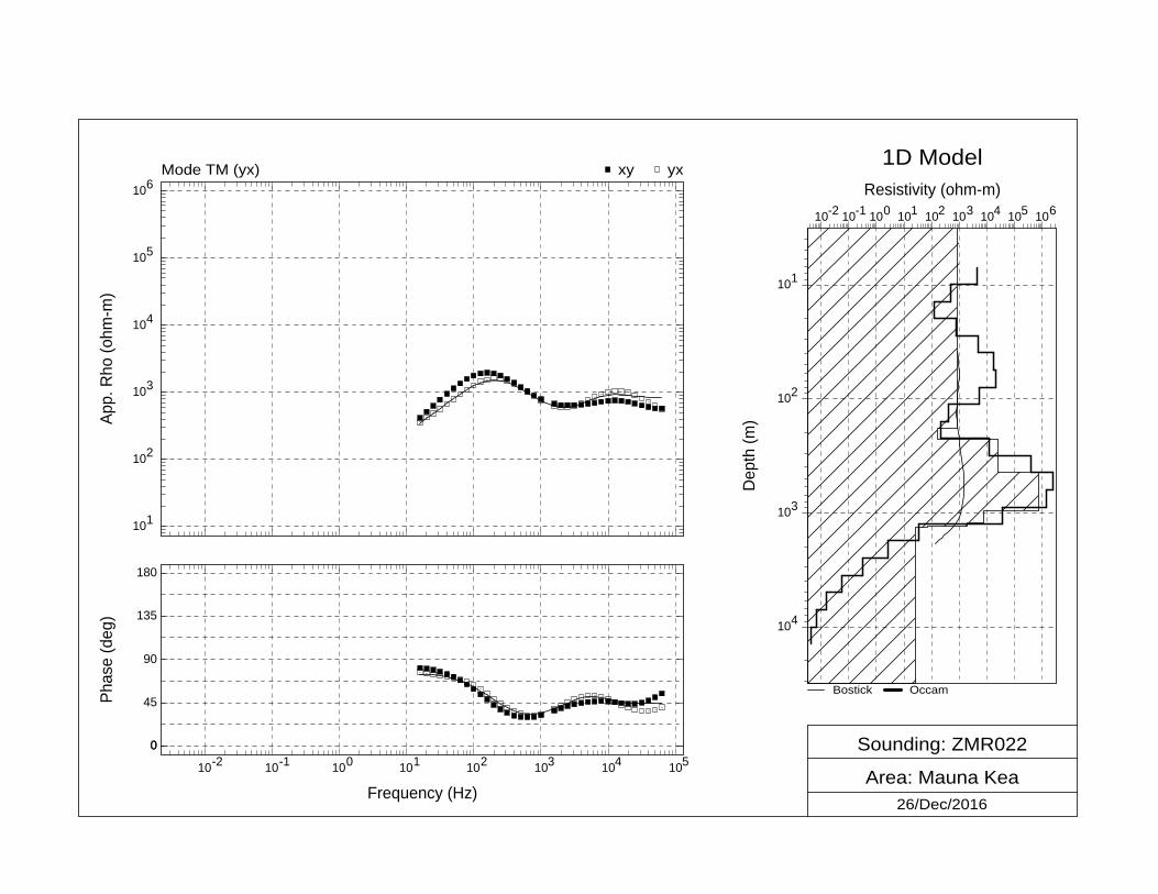
Sounding: ZMR022
Area: Mauna Kea26/Dec/2016
Mode TM (yx) yxxy1D Model
Bostick Occam
106
105
104
103
102
101
App.
Rho
(ohm
-m)
10-2 10-1 100 101 102 103 104 105
Frequency (Hz)
180
0
135
90
45
0
Phas
e (d
eg)
10-2 10-1 100 101 102 103 104 105 106Resistivity (ohm-m)
101
102
103
104
Dep
th (m
)

Sounding: ZMR023
Area: Mauna Kea26/Dec/2016
Mode TM (yx) yxxy1D Model
Bostick Occam
106
105
104
103
102
101
App.
Rho
(ohm
-m)
10-2 10-1 100 101 102 103 104 105
Frequency (Hz)
180
0
135
90
45
0
Phas
e (d
eg)
10-710-610-510-410-310-210-1100101102103104105106Resistivity (ohm-m)
101
102
103
104
Dep
th (m
)
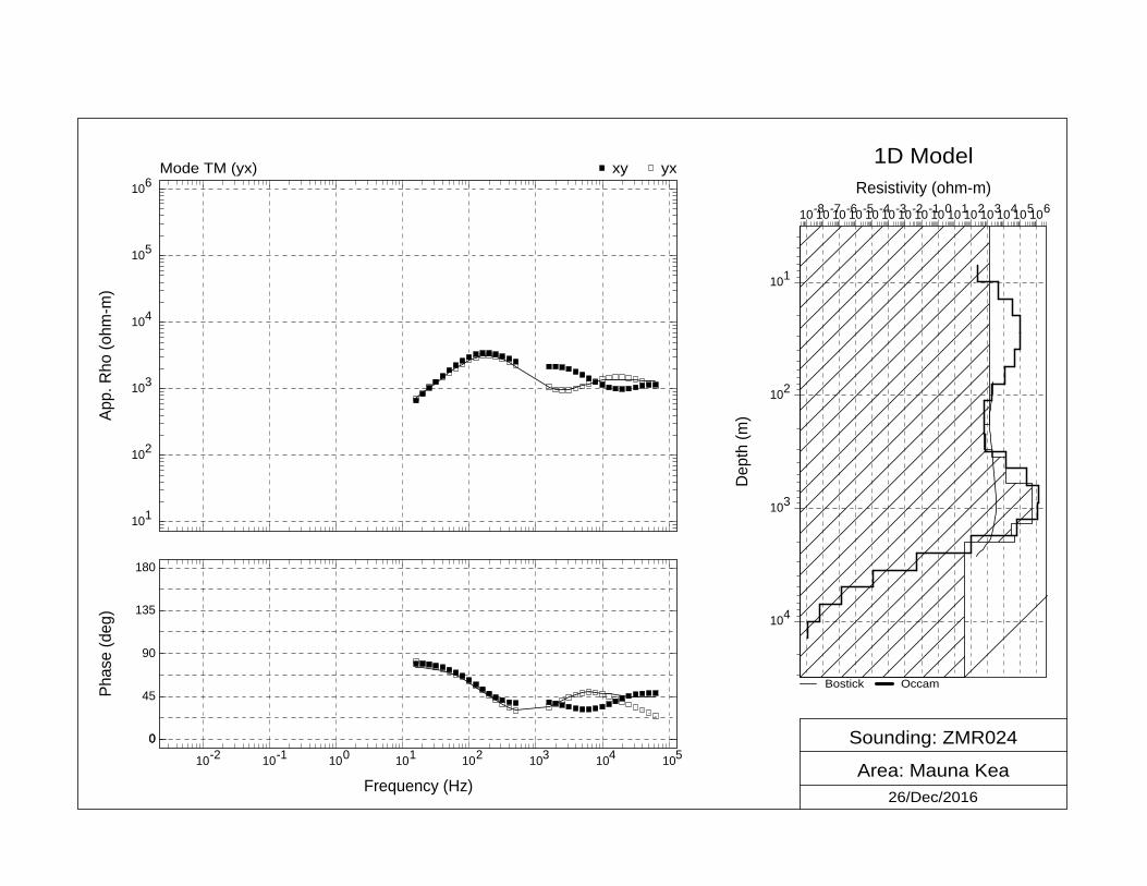
Sounding: ZMR024
Area: Mauna Kea26/Dec/2016
Mode TM (yx) yxxy1D Model
Bostick Occam
106
105
104
103
102
101
App.
Rho
(ohm
-m)
10-2 10-1 100 101 102 103 104 105
Frequency (Hz)
180
0
135
90
45
0
Phas
e (d
eg)
10-810-710-610-510-410-310-210-1100101102103104105106Resistivity (ohm-m)
101
102
103
104
Dep
th (m
)

Sounding: ZMR025
Area: Mauna Kea26/Dec/2016
Mode TM (yx) yxxy1D Model
Bostick Occam
106
105
104
103
102
101
App.
Rho
(ohm
-m)
10-2 10-1 100 101 102 103 104 105
Frequency (Hz)
180
0
135
90
45
0
Phas
e (d
eg)
102 103 104 105 106 107 108Resistivity (ohm-m)
101
102
103
104
Dep
th (m
)
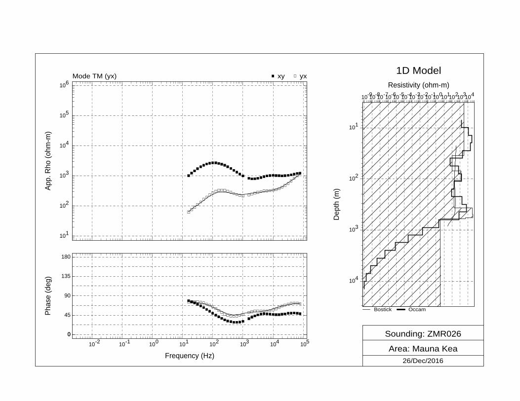
Sounding: ZMR026
Area: Mauna Kea26/Dec/2016
Mode TM (yx) yxxy1D Model
Bostick Occam
106
105
104
103
102
101
App.
Rho
(ohm
-m)
10-2 10-1 100 101 102 103 104 105
Frequency (Hz)
180
0
135
90
45
0
Phas
e (d
eg)
10-910-810-710-610-510-410-310-210-1100101102103104Resistivity (ohm-m)
101
102
103
104
Dep
th (m
)
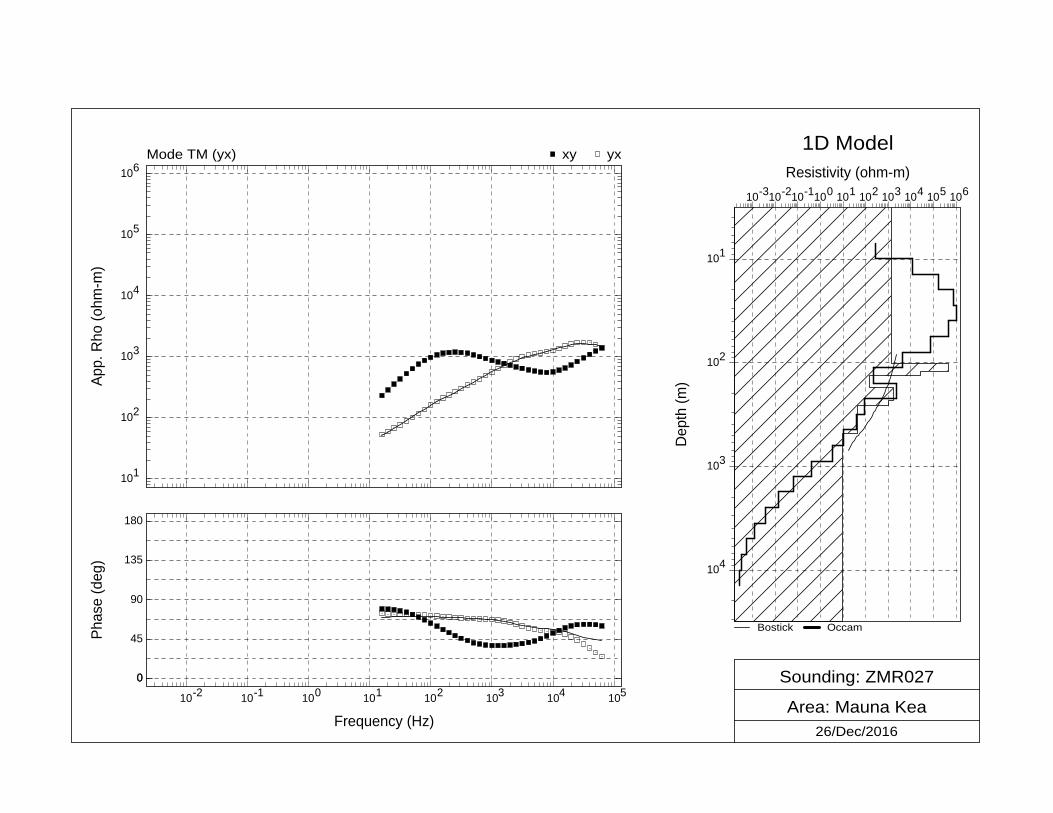
Sounding: ZMR027
Area: Mauna Kea26/Dec/2016
Mode TM (yx) yxxy1D Model
Bostick Occam
106
105
104
103
102
101
App.
Rho
(ohm
-m)
10-2 10-1 100 101 102 103 104 105
Frequency (Hz)
180
0
135
90
45
0
Phas
e (d
eg)
10-310-210-1100 101 102 103 104 105 106Resistivity (ohm-m)
101
102
103
104
Dep
th (m
)

Sounding: ZMR028
Area: Mauna Kea26/Dec/2016
Mode TM (yx) yxxy1D Model
Bostick Occam
106
105
104
103
102
101
App.
Rho
(ohm
-m)
10-2 10-1 100 101 102 103 104 105
Frequency (Hz)
180
0
135
90
45
0
Phas
e (d
eg)
103 104 105 106 107 108Resistivity (ohm-m)
101
102
103
104
Dep
th (m
)
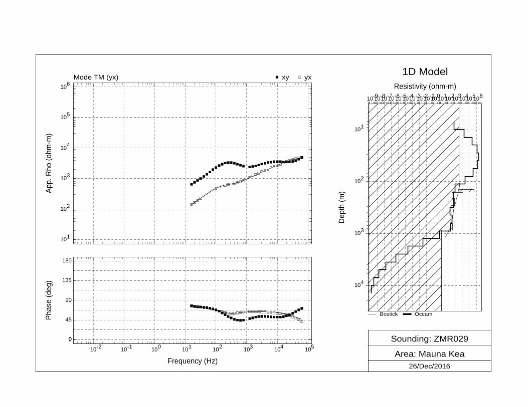
Sounding: ZMR029
Area: Mauna Kea26/Dec/2016
Mode TM (yx) yxxy1D Model
Bostick Occam
106
105
104
103
102
101
App.
Rho
(ohm
-m)
10-2 10-1 100 101 102 103 104 105
Frequency (Hz)
180
0
135
90
45
0
Phas
e (d
eg)
10-910-810-710-610-510-410-310-210-1100101102103104105106Resistivity (ohm-m)
101
102
103
104
Dep
th (m
)

Sounding: ZMR030
Area: Mauna Kea26/Dec/2016
Mode TM (yx) yxxy1D Model
Bostick Occam
106
105
104
103
102
101
App.
Rho
(ohm
-m)
10-2 10-1 100 101 102 103 104 105
Frequency (Hz)
180
0
135
90
45
0
Phas
e (d
eg)
10-210-1100 101 102 103 104 105 106 107Resistivity (ohm-m)
101
102
103
104
Dep
th (m
)

Sounding: ZMR031
Area: Mauna Kea26/Dec/2016
Mode TM (yx) yxxy1D Model
Bostick Occam
106
105
104
103
102
101
App.
Rho
(ohm
-m)
10-2 10-1 100 101 102 103 104 105
Frequency (Hz)
180
0
135
90
45
0
Phas
e (d
eg)
10-610-510-410-310-210-1100101102103104105Resistivity (ohm-m)
101
102
103
104
Dep
th (m
)

Sounding: ZMR032
Area: Mauna Kea26/Dec/2016
Mode TM (yx) yxxy1D Model
Bostick Occam
106
105
104
103
102
101
App.
Rho
(ohm
-m)
10-2 10-1 100 101 102 103 104 105
Frequency (Hz)
180
0
135
90
45
0
Phas
e (d
eg)
10-3 10-2 10-1 100 101 102 103 104 105Resistivity (ohm-m)
101
102
103
104
Dep
th (m
)

Sounding: ZMR033
Area: Mauna Kea26/Dec/2016
Mode TM (yx) yxxy1D Model
Bostick Occam
106
105
104
103
102
101
App.
Rho
(ohm
-m)
10-2 10-1 100 101 102 103 104 105
Frequency (Hz)
180
0
135
90
45
0
Phas
e (d
eg)
10-610-510-410-310-210-1100101102103104105Resistivity (ohm-m)
101
102
103
104
Dep
th (m
)

Sounding: ZMR034
Area: Mauna Kea26/Dec/2016
Mode TM (yx) yxxy1D Model
Bostick Occam
106
105
104
103
102
101
App.
Rho
(ohm
-m)
10-2 10-1 100 101 102 103 104 105
Frequency (Hz)
180
0
135
90
45
0
Phas
e (d
eg)
10-310-210-1100 101 102 103 104 105 106Resistivity (ohm-m)
101
102
103
104
Dep
th (m
)

Sounding: ZMR035
Area: Mauna Kea26/Dec/2016
Mode TM (yx) yxxy1D Model
Bostick Occam
106
105
104
103
102
101
App.
Rho
(ohm
-m)
10-2 10-1 100 101 102 103 104 105
Frequency (Hz)
180
0
135
90
45
0
Phas
e (d
eg)
10-710-610-510-410-310-210-1100101102103104105Resistivity (ohm-m)
101
102
103
104
Dep
th (m
)

Sounding: ZMR036
Area: Mauna Kea26/Dec/2016
Mode TM (yx) yxxy1D Model
Bostick Occam
106
105
104
103
102
101
App.
Rho
(ohm
-m)
10-2 10-1 100 101 102 103 104 105
Frequency (Hz)
180
0
135
90
45
0
Phas
e (d
eg)
102 103 104 105 106 107 108Resistivity (ohm-m)
101
102
103
104
Dep
th (m
)
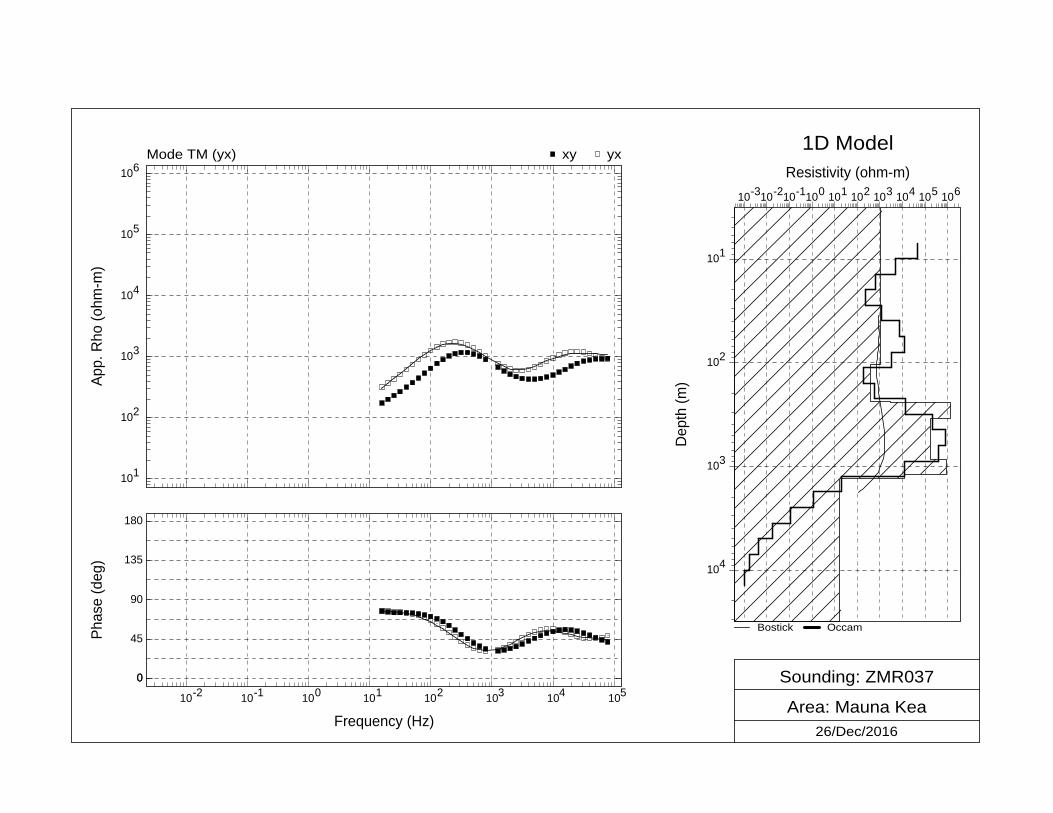
Sounding: ZMR037
Area: Mauna Kea26/Dec/2016
Mode TM (yx) yxxy1D Model
Bostick Occam
106
105
104
103
102
101
App.
Rho
(ohm
-m)
10-2 10-1 100 101 102 103 104 105
Frequency (Hz)
180
0
135
90
45
0
Phas
e (d
eg)
10-310-210-1100 101 102 103 104 105 106Resistivity (ohm-m)
101
102
103
104
Dep
th (m
)
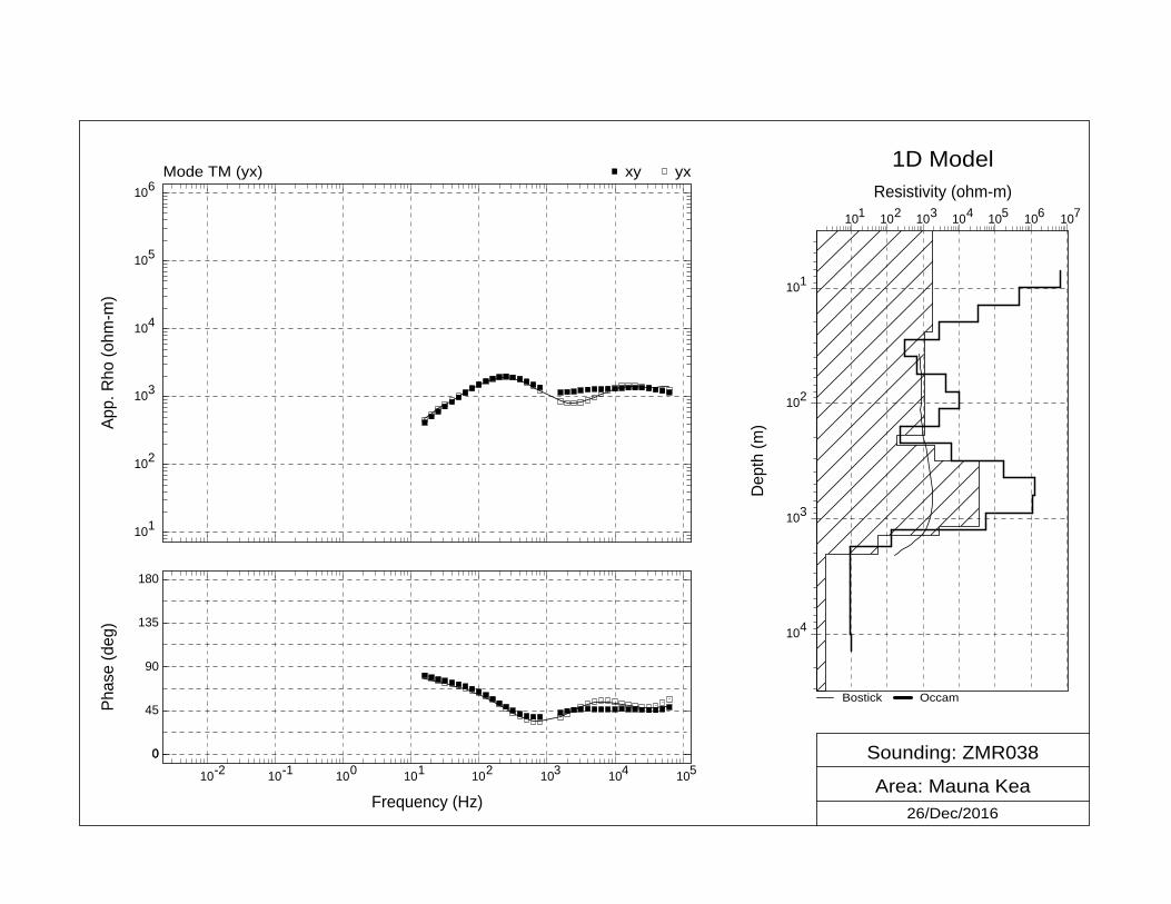
Sounding: ZMR038
Area: Mauna Kea26/Dec/2016
Mode TM (yx) yxxy1D Model
Bostick Occam
106
105
104
103
102
101
App.
Rho
(ohm
-m)
10-2 10-1 100 101 102 103 104 105
Frequency (Hz)
180
0
135
90
45
0
Phas
e (d
eg)
101 102 103 104 105 106 107Resistivity (ohm-m)
101
102
103
104
Dep
th (m
)

Sounding: ZMR039
Area: Mauna Kea26/Dec/2016
Mode TM (yx) yxxy1D Model
Bostick Occam
106
105
104
103
102
101
App.
Rho
(ohm
-m)
10-2 10-1 100 101 102 103 104 105
Frequency (Hz)
180
0
135
90
45
0
Phas
e (d
eg)
10-310-210-1100 101 102 103 104 105 106Resistivity (ohm-m)
101
102
103
104
Dep
th (m
)
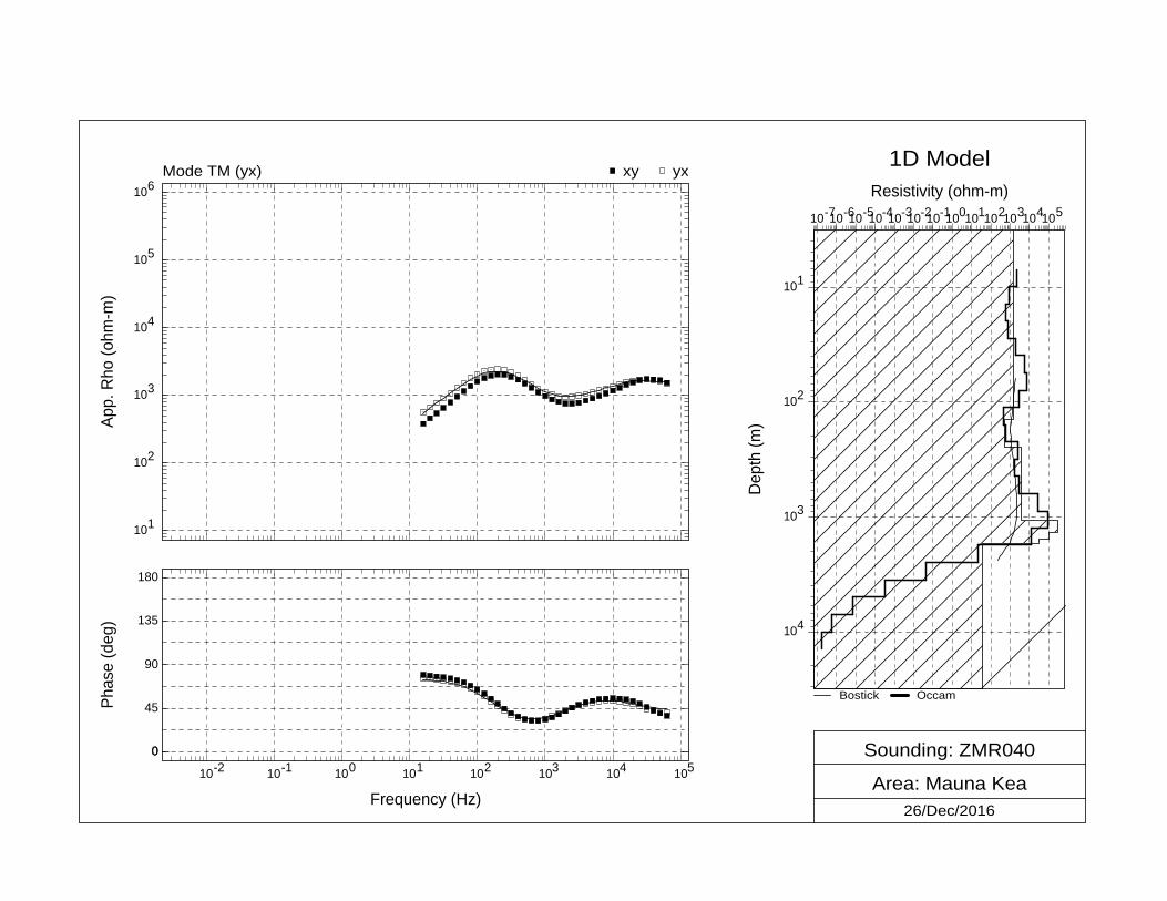
Sounding: ZMR040
Area: Mauna Kea26/Dec/2016
Mode TM (yx) yxxy1D Model
Bostick Occam
106
105
104
103
102
101
App.
Rho
(ohm
-m)
10-2 10-1 100 101 102 103 104 105
Frequency (Hz)
180
0
135
90
45
0
Phas
e (d
eg)
10-710-610-510-410-310-210-1100101102103104105Resistivity (ohm-m)
101
102
103
104
Dep
th (m
)
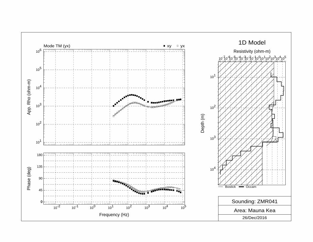
Sounding: ZMR041
Area: Mauna Kea26/Dec/2016
Mode TM (yx) yxxy1D Model
Bostick Occam
106
105
104
103
102
101
App.
Rho
(ohm
-m)
10-2 10-1 100 101 102 103 104 105
Frequency (Hz)
180
0
135
90
45
0
Phas
e (d
eg)
10-710-610-510-410-310-210-1100101102103104105Resistivity (ohm-m)
101
102
103
104
Dep
th (m
)

Sounding: ZMR042
Area: Mauna Kea26/Dec/2016
Mode TM (yx) yxxy1D Model
Bostick Occam
106
105
104
103
102
101
App.
Rho
(ohm
-m)
10-2 10-1 100 101 102 103 104 105
Frequency (Hz)
180
0
135
90
45
0
Phas
e (d
eg)
10-1210-1110-1010-910-810-710-610-510-410-310-210-1100101102103104105Resistivity (ohm-m)
101
102
103
104
Dep
th (m
)
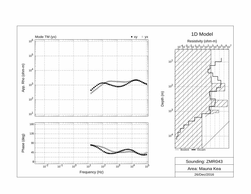
Sounding: ZMR043
Area: Mauna Kea26/Dec/2016
Mode TM (yx) yxxy1D Model
Bostick Occam
106
105
104
103
102
101
App.
Rho
(ohm
-m)
10-2 10-1 100 101 102 103 104 105
Frequency (Hz)
180
0
135
90
45
0
Phas
e (d
eg)
10-410-310-210-1100101102103104105106107Resistivity (ohm-m)
101
102
103
104
Dep
th (m
)

Sounding: ZMR044
Area: Mauna Kea26/Dec/2016
Mode TM (yx) yxxy1D Model
Bostick Occam
106
105
104
103
102
101
App.
Rho
(ohm
-m)
10-2 10-1 100 101 102 103 104 105
Frequency (Hz)
180
0
135
90
45
0
Phas
e (d
eg)
10-4 10-3 10-2 10-1 100 101 102 103 104Resistivity (ohm-m)
101
102
103
104
Dep
th (m
)

Sounding: ZMR045
Area: Mauna Kea26/Dec/2016
Mode TM (yx) yxxy1D Model
Bostick Occam
106
105
104
103
102
101
App.
Rho
(ohm
-m)
10-2 10-1 100 101 102 103 104 105
Frequency (Hz)
180
0
135
90
45
0
Phas
e (d
eg)
10-610-510-410-310-210-1100 101 102103 104Resistivity (ohm-m)
101
102
103
104
Dep
th (m
)

Sounding: ZMR046
Area: Mauna Kea26/Dec/2016
Mode TM (yx) yxxy1D Model
Bostick Occam
106
105
104
103
102
101
App.
Rho
(ohm
-m)
10-2 10-1 100 101 102 103 104 105
Frequency (Hz)
180
0
135
90
45
0
Phas
e (d
eg)
10-810-710-610-510-410-310-210-1100101102103104105106Resistivity (ohm-m)
101
102
103
104
Dep
th (m
)

Sounding: ZMR047
Area: Mauna Kea26/Dec/2016
Mode TM (yx) yxxy1D Model
Bostick Occam
106
105
104
103
102
101
App.
Rho
(ohm
-m)
10-2 10-1 100 101 102 103 104 105
Frequency (Hz)
180
0
135
90
45
0
Phas
e (d
eg)
102 103 104 105 106Resistivity (ohm-m)
101
102
103
104
Dep
th (m
)
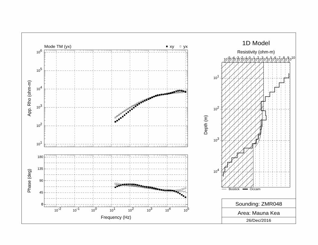
Sounding: ZMR048
Area: Mauna Kea26/Dec/2016
Mode TM (yx) yxxy1D Model
Bostick Occam
106
105
104
103
102
101
App.
Rho
(ohm
-m)
10-2 10-1 100 101 102 103 104 105
Frequency (Hz)
180
0
135
90
45
0
Phas
e (d
eg)
10-510-410-310-210-11001011021031041051061071081091010Resistivity (ohm-m)
101
102
103
104
Dep
th (m
)

Sounding: ZMR049
Area: Mauna Kea26/Dec/2016
Mode TM (yx) yxxy1D Model
Bostick Occam
106
105
104
103
102
101
App.
Rho
(ohm
-m)
10-2 10-1 100 101 102 103 104 105
Frequency (Hz)
180
0
135
90
45
0
Phas
e (d
eg)
101 102 103 104 105 106Resistivity (ohm-m)
101
102
103
104
Dep
th (m
)

Sounding: ZMR051
Area: Mauna Kea26/Dec/2016
Mode TM (yx) yxxy1D Model
Bostick Occam
106
105
104
103
102
101
App.
Rho
(ohm
-m)
10-2 10-1 100 101 102 103 104 105
Frequency (Hz)
180
0
135
90
45
0
Phas
e (d
eg)
10-1 100 101 102 103 104Resistivity (ohm-m)
101
102
103
104
Dep
th (m
)

Sounding: ZMR052
Area: Mauna Kea26/Dec/2016
Mode TM (yx) yxxy1D Model
Bostick Occam
106
105
104
103
102
101
App.
Rho
(ohm
-m)
10-2 10-1 100 101 102 103 104 105
Frequency (Hz)
180
0
135
90
45
0
Phas
e (d
eg)
10-1 100 101 102 103 104 105Resistivity (ohm-m)
101
102
103
104
Dep
th (m
)

Sounding: ZMR053
Area: Mauna Kea26/Dec/2016
Mode TM (yx) yxxy1D Model
Bostick Occam
106
105
104
103
102
101
App.
Rho
(ohm
-m)
10-2 10-1 100 101 102 103 104 105
Frequency (Hz)
180
0
135
90
45
0
Phas
e (d
eg)
10-510-410-310-210-1100101102103104105106107108Resistivity (ohm-m)
101
102
103
104
Dep
th (m
)
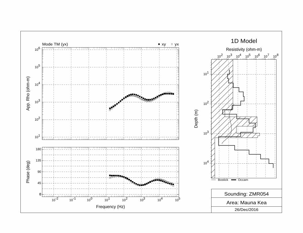
Sounding: ZMR054
Area: Mauna Kea26/Dec/2016
Mode TM (yx) yxxy1D Model
Bostick Occam
106
105
104
103
102
101
App.
Rho
(ohm
-m)
10-2 10-1 100 101 102 103 104 105
Frequency (Hz)
180
0
135
90
45
0
Phas
e (d
eg)
102 103 104 105 106 107 108Resistivity (ohm-m)
101
102
103
104
Dep
th (m
)

Sounding: ZMR055
Area: Mauna Kea26/Dec/2016
Mode TM (yx) yxxy1D Model
Bostick Occam
106
105
104
103
102
101
App.
Rho
(ohm
-m)
10-2 10-1 100 101 102 103 104 105
Frequency (Hz)
180
0
135
90
45
0
Phas
e (d
eg)
102 103 104 105 106 107 108 109Resistivity (ohm-m)
101
102
103
104
Dep
th (m
)

Sounding: ZMR056
Area: Mauna Kea26/Dec/2016
Mode TM (yx) yxxy1D Model
Bostick Occam
106
105
104
103
102
101
App.
Rho
(ohm
-m)
10-2 10-1 100 101 102 103 104 105
Frequency (Hz)
180
0
135
90
45
0
Phas
e (d
eg)
101 102 103 104 105 106 107 108 109 1010Resistivity (ohm-m)
101
102
103
104
Dep
th (m
)
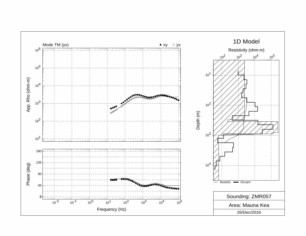
Sounding: ZMR057
Area: Mauna Kea26/Dec/2016
Mode TM (yx) yxxy1D Model
Bostick Occam
106
105
104
103
102
101
App.
Rho
(ohm
-m)
10-2 10-1 100 101 102 103 104 105
Frequency (Hz)
180
0
135
90
45
0
Phas
e (d
eg)
102 103 104 105Resistivity (ohm-m)
101
102
103
104
Dep
th (m
)