final report on nasa ames grant no. ncc2 - 5064 … ames grant no. ncc2 - 5064 ... 1.3 practical...
TRANSCRIPT
Final Report on
NASA Ames Grant No. NCC2 - 5064
Development of Multiobjective Optimization Techniques for Sonic
Boom Minimization
Technical Monitor: Dr. Eugene Tu
Performance Period:
5/16/94 9/15/96
Principal Investigators:
Aditi Chattopadhyay, Associate Professor,
Department of Mechanical and Aerospace Engineering
and
John Narayan Rajadas, Assistant Professor,
Department of Manufacturing and Aeronautical Engineering Technology
Graduate Research Associate:
Narayanan S. Pagaldipti
Department of Mechanical and Aerospace Engineering
Arizona State University
Tempe, Arizona 85287-6106
DECEMBER 1996
https://ntrs.nasa.gov/search.jsp?R=19970011407 2018-06-22T03:43:12+00:00Z

.
.
3.
.
,
TABLE OF CONTENTS
Topic Page
Abstract ............................................................................. 1
Introduction ......................................................................... 2
1.1 Multidisciplinary Design Optimization (MDO) .......................... 2
1.1.1 MDO Using Multilevel Decomposition .......................... 3
1.1.2 Accuracy of MDO Procedures .................................... 4
1.2 Design Sensitivity Analysis ................................................ 5
1.2.1 Semi-Analytical Sensitivity Analysis ............................ 5
1.2.2 Grid Sensitivity Analysis .......................................... 6
1.3 Practical Applications of MDO ............................................ 7
Objectives ........................................................................... 9
Sensitivity Analysis ................................................................ 10
3.1 Finite Difference Sensitivity Analysis .................................... 10
3.2 Discrete Semi-Analytical Aerodynamic Sensitivity Analysis ........... 10
3.3. Grid Sensitivity Technique ................................................. 12
3.4 Adaptation of Sensitivity Analysis to Flow Solver ...................... 15
3.5 Design Sensitivity Calculations for Wing-Body Configurations ...... 20
Optimization Techniques .......................................................... 26
4.1 Multilevel Decomposition .................................................. 26
4.2 Multiobjective Formulations ............................................... 28
4.2.1 Kreisselmeier-Steinhauser (K-S) Function Approach ......... 28
4.2.2 Modified Global Criteria Approach .............................. 30
4.3 Approximate Analysis ...................................................... 31
Applications of Multidisciplinary Design Optimization ........................ 32
5.1 Aerodynamic Optimization of a Theoretical Minimum Drag Body .... 32
5.1.1 Haack-Adam (H-A) Body ......................................... 32
5.1.2 Results and Discussion ............................................ 34
5.2 Multidisciplinary Optimization of High Speed
Wing-Body Configurations ................................................ 36
5.2.1 Multilevel Optimization Formulation ............................. 36
5.2.2 Wing-Body Configuration ........................................ 38
5.2.3 Wing Structural Model ............................................ 38
5.35.3.1
5.3.2
5.3.3
5.3.4
5.3.5
5.3.6
5.2.4 ResultsandDiscussion............................................
IntegratedAerodynamic/SonicBoomOptimization.....................Sonic Boom Analysis ..............................................Sonic Boom Sensitivities..........................................
OptimizationFormulation.........................................
Wing-BodyConfigurations.......................................
DeltaWing-BodyOptimization...................................
DoublySweptWing-BodyOptimization........................
5.4 IntegratedAerodynamic/SonicBoom/StructuralOptimization.........
5.4.1 OptimizationFormulation .........................................
5.4.2 Wing-Body Configuration ........................................
5.4.3 Structural Model and Analysis ....................................
5.4.4 Aerodynamic Load Calculations ..................................
5.4.5 Weight Calculations ................................................
5.4.6 Optimization Algorithms ..........................................
5.4.7 Results and Discussion ............................................
6. Concluding Remarks ..............................................................
References ........................................................................................
39
42
43
45
45
46
48
58
62
62
64
64
67
68
69
70
79
81
ii
List of Tables
Table Page
1 Grid sensitivity of the three-dimensional hyperbolic grid ......................... 21
2 Sensitivity of the drag coefficient, (dCD/d0i) ....................................... 24
3 Sensitivity of the lift coefficient (dCL/d_i) .......................................... 24
4 Comparison of design variables and objective function ........................... 35
5 Aerodynamic design variables ........................................................ 40
6 Structural design variables ............................................................ 42
7 Delta wing-body case; near field optimization with lift coefficient constraint... 49
8 Delta wing-body case; near field optimization without
lift coefficient constraint ............................................................... 52
9 Delta wing-body case; far field optimization without lift coefficient constraint. 56
10 Doubly swept wing-body case; near field case with lift coefficient constraint.. 58
11 Comparison of level 1 design variables and objective functions .................. 72
12 Comparison of level 2 design variables and objective function(s) ................ 75
°o°
111

List of Figures
Figure
1
2
3
4
5
6a
6b
7
8
9
10
11
12
13
14
15
16
17
18a
18b
19
2O
21a
21b
Coordinate systems ....................................................................
Delta wing-body configuration (schematic) .........................................
Comparison of CPU time (seconds) for the sensitivity of hyperbolic grid ......
Comparison of CPU time for aerodynamic sensitivity analysis ..................
Two level decomposition (schematic) ................................................
Original objective functions and constraints .........................................
K-S function envelope .................................................................
Haack-Adam body .....................................................................
Comparison of wave drag coefficient ................................................
Comparison of reference and optimum body configurations ......................
Wing cross-section and wing spar (box beam) .....................................
Iteration history of drag coefficient (CDu) ...........................................
Iteration history of lift coefficient (CLu) .............................................
Iteration history of weight .............................................................
Sonic boom pressure signature of a supersonic wing-body configuration ......
Doubly swept wing-body configuration (schematic) ...............................
Comparison of geometries;
near field optimization with lift coefficient constraint ..............................
Comparison of objective functions;
near field optimization with lift coefficient constraint ..............................
Comparison of pressure signatures;
near field optimization with lift coefficient constraint; d! -- 3.61 lb ..............
Comparison of pressure signatures; near field optimization with lift
coefficient constraint; extrapolated to ground level (dl = 941.7 lb) ..............
Comparison of geometries;
near field optimization without lift coefficient constraint ..........................
Comparison of objective functions;
near field case without lift coefficient constraint ....................................
Comparison of pressure signatures;
near field optimization without lift coefficient constraint; dl = 3.61 lb ...........
Comparison of pressure signatures; near field optimization without lift
coefficient constraint; extrapolated to ground level (dl = 941.7 lb) ..............
Page
12
22
23
25
27
30
3O
33
35
36
39
40
40
41
43
47
5O
5O
51
51
53
53
54
54
iv

22 Comparison of geometries; far field case without lift coefficient constraint ..... 56
23 Comparison of objective functions;
far field case without lift coefficient constraint ...................................... 57
24 Comparison of pressure signatures;
far field case without lift coefficient constraint ...................................... 57
25 Comparison of planforms; near field case with lift coefficient constraint ........ 60
26 Comparison of objective functions;
near field case with lift coefficient constraint ........................................ 60
27a Comparison of pressure signatures;
near field optimization with lift coefficient constraint; d l = 3.61 lb .............. 61
27b Comparison of pressure signatures; near field case with lift
coefficient constraint; extrapolated to ground level (dl = 941.7 lb) .............. 61
28 Nodal force vectors due to aerodynamic loading at a given wing section ....... 64
29 Composite box beam model ........................................................... 65
30 Finite element degrees of freedom .................................................... 66
31 Comparison of planforms; near field optimization ................................. 71
32 Comparison of level 1 objective functions .......................................... 73
33 Comparison of pressure signatures; near field optimization ....................... 73
34 Comparison of level 2 objective function(s) ........................................ 75
35 Comparison of normalized root stresses and bending moments .................. 77
36 Comparison of planforms; far field optimization ................................... 77
37 Comparison of pressure signatures; far field optimization ........................ 78
V

CD
CDu
CDw
CL
CLu
Co
Ct
d
F
Fi
FKS
gj
lb
In
Mx
My
Moo
NDV
R
r
rm
T
tc
U
V
W
Wfus
Wwsk
Wwsp
Nomenclature
inviscid drag coefficient (non-dimensionalized using wing planform area) of
wing-body configuration
inviscid drag coefficient (non-dimensionalized using unit reference area) of
delta wing-body configuration
wave drag coefficient (non-dimensionalized using maximum cross-sectional
area) of Hack-Adam body
inviscid lift coefficient (non-dimensionalized using wing planform area) of
wing-body configurations
inviscid lift coefficient (non-dimensionalized using unit reference area) of
delta wing-body configuration
root chord
tip chord
vertical distance from the axis of aircraft
vector of objective functions
i_ objective function
Kreisselmeier-Steinhauser function
jth constraint
aircraft length
nose length
out of plane bending moment on wing
in plane bending moment on wing
freestream Mach number
number of design variables
vector of discrete flow equations
radius of centerbody
maximum nose radius
torsion on the wing
wing thickness-to-chord ratio
x-component velocity
y-component velocity
aircraft weight
fuselage weight
wing skin weight
wing spar weight
vi

w
Ws
X
Xb
Xw
Y
z
Ap
0
Om
n
K
)-I
).2
P
0
Subscripts
max, u
rain, 1
z-component velocity
wing span
streamwise coordinate
break length
wing starting location
tangential coordinate
spanwise coordinate
change in pressure from freestream value, normalized by freestream value
design variable vector
m th design variable
tangential coordinate
thermal conductivity of air
leading edge sweep (delta wing-body case)
first leading edge sweep (doubly swept wing-body case)
second leading edge sweep (doubly swept wing-body case)
density of air
vector of normal and shear stresses in wing box beam
streamwise coordinate
normal coordinate
upper bound
lower bound
free stream condition
vii


Abstract
A discrete, semi-analytical sensitivity analysis procedure has been developed for calculating
aerodynamic design sensitivities. The sensitivities of the flow variables and the grid coordinates
are numerically calculated using direct differentiation of the respective discretized governing
equations. The sensitivity analysis techniques are adapted within a parabolized Navier Stokes
equations solver. Aerodynamic design sensitivities for high speed wing-body configurations are
calculated using the semi-analytical sensitivity analysis procedures. Representative results obtained
compare well with those obtained using the finite difference approach and establish the
computational efficiency and accuracy of the semi-analytical procedures.
Multidisciplinary design optimization procedures have been developed for aerospace
applications namely, gas turbine blades and high speed wing-body configurations. In complex
applications, the coupled optimization problems are decomposed into sublevels using multilevel
decomposition techniques. In cases with multiple objective functions, formal multiobjective
formulation such as the Kreisselmeier-Steinhauser function approach and the modified global
criteria approach have been used. Nonlinear programming techniques for continuous design
variables and a hybrid optimization technqiue, based on a simulated annealing algorithm, for
discrete design variables have been used for solving the optimization problems.
The optimization procedure for gas turbine blades improves the aerodynamic and heat
transfer characteristics of the blades. The two-dimensional, blade-to-blade aerodynamic analysis is
performed using a panel code. The blade heat transfer analysis is performed using an in-house
developed finite element procedure. The optimization procedure yields blade shapes with
significantly improved velocity and temperature distributions.
The multidisciplinary design optimization procedures for high speed wing-body
configurations simultaneously improve the aerodynamic, the sonic boom and the structural
characteristics of the aircraft. The flow solution is obtained using a comprehensive parabolized
Navier Stokes solver. Sonic boom analysis is performed using an extrapolation procedure. The
aircraft wing load carrying member is modeled as either an isotropic or a composite box beam.
The isotropic box beam is analyzed using thin wall theory. The composite box beam is analyzed
using a finite element procedure. The developed optimization procedures yield significant
improvements in all the performance criteria and provide interesting design trade-offs. The semi-
analytical sensitivity analysis techniques offer significant computational savings and allow the use
of comprehensive analysis procedures within design optimization studies.
1. Introduction
Design of aerospace vehicles is associated with complex multidisciplinary couplings. The
design process inherently involves interactions between various disciplines of engineering such as
aerodynamics, structures, dynamics, aeroelasticity, heat transfer, controls and acoustics. Also, the
impact of the operation of aerospace vehicles on the environment is gaining attention and
importance at all stages of the design process. Examples of factors that have environmental impact
include the engine noise, sonic boom, emission effects etc. The final vehicle configuration has to
satisfy a number of design requirements associated with the various disciplines. Often, these
multidisciplinary requirements are conflicting in nature. Design requirements that enhance the
performance of the aerospace system in one discipline, may deteriorate its performance in other
disciplines. For example, in high speed aircraft, it is desirable to have slender wings and a slender
fuselage from aerodynamics point of view. From a structural view point, it is necessary to have a
sufficiently thick wing to carry the aerodynamic loading well within material limits. From a
payload point of view, the fuselage has to have a minimum volume to accomodate an economically
feasible amount of payload. These are examples of conflicting design requirements. Also, the
impact of individual design features on the overall system performance is often not apparent to the
designer. Therefore, the designer must be able to evaluate the various conflicting design
requirements and provide insight into the effect of each design feature on the overall performance
of the system. In a typical aircraft design procedure, these conflicting design requirements are
compromised through a trade-off study. With the advent of modern computer technology,
Multidisciplinary Design Optimization (MDO) techniques could be well suited for such design
trade-off studies.
1.1 Multidisciplinary Design Optimization (MDO)
Multidisciplinary design optimization involves the coupling of two or more disciplines,
associated with the design of a sytem, within a closed loop numerical optimization procedure. The
importance of multidisciplinary couplings in successful design optimization of aerospace systems
has been long recognized. Sobieszczanski and Loendorf [ 1] developed a MDO procedure for the
design of fuselage structures. Fulton et al. [2] performed design optimization of a complete aircraft
model that involved 700 design variables and 2500 constraints. Barthelemy et al. [3-5] developed
MDO procedures for supersonic transport aircraft which included structural, aerodynamic and
aeroelastic criteria. Celi and Friedmann [6] developed a MDO procedure that performed structural
optimization of rotor blades with constraints on their aeroelastic behavior. Chattopadhyay et al. [7-
12] and McCarthy et al. [ 13-14] have developed several MDO procedures that integrate structural,
aeroelastic and aerodynamic performance criteria for various rotary wing applications. In these
2

researchefforts,optimizationis performedby addressingall thedesigncriteria in a single level.
Suchanoptimizationapproach,referredto asthe"individual disciplinefeasible"formulation [15-16], can be inefficient and may restrict designvariable movementdue to conflicting design
requirements.
1.1.1 MDO Using Multilevel Decomposition
A highly integrated and large design optimization problem can be decomposed into a
number of smaller subproblems using a process referred to as multilevel decomposition. The
subproblems are optimized separately and a procedure, which accounts for the interdisciplinary
coupling, is devised so that at convergence, the resulting optimum is that of the original non-
decomposed problem. Decomposition also helps decrease the size of the optimization problem
because each subproblem uses only a subset of the original design parameters as design variables.
For some problems, the process that accounts for interdisciplinary coupling may be non-iterative.
Multilevel decomposition techniques with a non-iterative interdisciplinary coupling process are
called hierarchical decomposition techniques [ 16]. For highly coupled systems, the process that
establishes interdisciplinary coupling is iterative in nature. Multilevel decomposition techniques
with such iterative coupling processes fall under non-hierarchical decomposition techniques [ 16].
Multilevel decomposition techniques have been widely applied to problems in structural
optimization. Schmit et al. [17-18] developed a hierarchical procedure for truss and wing box
models that included local and global constraints. Hughes [19] developed similar ideas for naval
structures. Sobieszczanski [20] developed a linear decomposition method for a large class of
nonlinear design problems. The effectiveness of this method has been demonstrated on two- and
three-level structural framework design problems [21-23]. Using the same method, Wrenn and
Dovi [24] optimized a complex transport wing model with 1200 variables and 2500 nonlinear
constraints. The method has been adapted to penalty function optimization techniques [25] where
improved efficiency is demonstrated by limiting the optimization to a single minimization step for
each subproblem within each cycle. Kirsch [26] used a multilevel formulation for the simultaneous
analysis and optimization of reinforced concrete beams. An obstacle to the use of multilevel
methods is that they can be computationally expensive because of the cycling necessary to account
for the coupling between the subproblems. Barthelemy and Riley [27] developed an improved
approach that increases the computational efficiency of multilevel optimization by adopting
constraint approximation and temporary constraint deletion. Barthelemy [28] reviewed various
engineering applications of heuristic decomposition methods. Bloebaum and Hajela [29] have
applied these methods for the decomposition of non-hierarchical systems.

Attempts havealso beenmadeto usemultilevel decompositiontechniquesfor MDO
problems.RoganandKolb [30] showedhow atransportaircraftpreliminarydesignproblemcanbe treatedasa multilevel optimizationproblem. Adelmanet al. [31] have reported a two-level
procedure for performing integrated aerodynamic, dynamic and structural optimization of rotor
blades, based on the multilevel optimization strategy described in Ref. 20. Chattopadhyay et al.
[32] developed a three-level, non-hierarchical procedure for optimization of helicopter rotor blades
with the integration of aerodynamics, dynamics, aeroelastic stability and structures. The blade
aerodynamic performance was improved in level 1, the dynamic performance and the aeroelastic
stability roots of the blade were improved in level 2 and the blade structural weight was reduced in
level 3 subject to stress constraints. Chattopadhyay et al. [33] also developed a two-level
decomposition procedure for improved high-speed cruise and hovering performance of tiltrotor
aircraft. These non-hierarchical multilevel optimization procedures cycle through the various levels
until global convergence is achieved. The interdisciplinary coupling between the various levels is
established through optimal sensitivity parameters [34-37]. At a given level, the optimal sensitivity
parameters are the derivatives of the objective functions and design variables of the other levels
with respect to design variables of the current level.
1.1.2 Accuracy of MDO Procedures
The validity of the designs obtained using MDO procedures depends strongly upon the
accuracy of the analysis techniques used. The reliability and practical implementation of the design
trends obtained from MDO procedures are critically dependent on the accuracy of the analysis
techniques used within them. It is essential to integrate accurate, efficient and comprehensive
analysis techniques within the MDO procedures so that the optimum designs obtained are
dependable. Such detailed analysis techniques are computationally intensive and therefore, can be
prohibitive within a design optimization environment. For example, in high speed aircraft design,
it is essential to use a comprehensive aerodynamic analysis procedure to solve the complex flow
field around the aircraft. Although accurate detailed analyses of many complex flow fields are now
possible using efficient Computational Fluid Dynamics (CFD) solvers and powerful
supercomputers, viscous-compressible flow calculations around supersonic aircraft can require
several Central Processing Unit (CPU) hours per steady-state solution. Therefore, the use of such
comprehensive analysis procedures within MDO can be computationally expensive, especially if
gradient-based techniques are used. Gradient-based optimization techniques require the calculation
of the derivatives of the objective functions and constraints of the optimization procedure with
respect to the design variables during each optimization cycle. The calculation of these derivatives
is termed sensitivity analysis. In a typical multidisciplinary optimization process, most of the
4

computationaleffort is spenttowardssensitivityanalysis. Thecomputationaltime requiredfor
performingsensitivityanalysisdirectlyincreaseswith (1) thecomplexityof theanalysisproceduresusedand(2) thenumberof designvariablesinvolved. SinceaccurateMDO procedurestypically
usecomprehensiveanalysisproceduresanda largenumberof designvariables,it is importantto
developanduseefficientsensitivityanalysistechniques.
1.2 Design Sensitivity Analysis
Sensitivity analysis, in which the derivative of a system performance function (e.g., the
lift-to-drag ratio of an aircraft wing) with respect to design variables (e.g., wing root chord) is
calculated, is an essential component in gradient-based design optimization. A widely used
technique for performing sensitivity analysis is the method of finite differences. In this method,
the performance function, whose derivatives with respect to design variables are to be calculated, is
first evaluated at the given design point. Then, the design variables are perturbed, one at a time
and the function is evaluated at each one of these perturbed design points. The derivatives of the
performance function are then calculated by taking the differences between perturbed function
values and the original function value and dividing these differences by the corresponding
perturbations in the design variables. As a result, the use of this method requires several
applications of the appropriate analysis procedures. For example, if there are NDV design
variables, then the finite difference method requires the execution of the analysis procedures at least
(NDV+I) times. Thus the associated computational cost can be prohibitive when this method is
used in an optimization problem involving a large number of design variables and computationally
intensive analysis procedures (such as CFD codes for evaluating three-dimensional flow fields).
Therefore, it is necessary to develop alternative techniques to calculate design sensitivities, so that
complex analysis procedures may be more useful as practical design tools in multidisciplinary
design optimization environments.
1.2.1 Semi-Analytical Sensitivity Analysis
It has been recognized that analytical or semi-analytical techniques for sensitivity analysis
are preferable over the finite difference method due to their computational efficiency and accuracy
[38]. Two such techniques are the direct differentiation approach and the adjoint variable approach
[39-43]. These techniques have been widely used for sensitivity calculations in structural
optimization [39-43]. In the direct differentiation approach, the governing equations for the
response variables (e. g., flow variables in a CFD procedure) are differentiated with respect to the
design variables using chain rule. This yields a large linear system of equations for the sensitivities
of the system response variables. The derivatives of the system performance functions are readily
5

calculatedfrom theseresponsesensitivities. In the adjoint variableapproach,adjoint variablevectorsareobtainedasthe solutionto anadjointproblem. Theadjoint variablevectorsarethen
usedto calculatethesensitivitiesof thesystemperformancefunctions. It is importantto notethat
in theadjoint variableapproach,thedesignsensitivitiesof thesystemresponsevariablesarenotcalculated.The two semi-analyticaltechniquesareequivalentandyield identicalresultsfor thesensitivities. Therehasbeena widespreadinterestin using thesetechniquesfor calculating
aerodynamicsensitivities. CarlsonandElbanna [44-47] have usedthe direct differentiation
techniqueon thediscretizedtransonicsmallperturbationandthefull potentialequationsto obtain
aerodynamicsensitivities. Baysalet al. [48-51]haveperformeddiscretesensitivity analysisbydirectlydifferentiatingthethree-dimensionalEulerequations.Korivi et al. [52] andNewmanetal.
[53] havedevelopeda semi-analyticalsensitivity analysisprocedurefor the thin-layerNavier-
Stokesequationsusinganincrementalstrategy.In thisapproach,theaerodynamicsensitivitiesarecalculatedin anincrementalfashionsimilarto theflow solution.
Dependingonthetypeof governingequationsused,semi-analyticalsensitivityanalysiscan
alsobecategorizedeitherasadiscreteapproach[44-54]or a continuousapproach[55-59]. The
discreteapproachtakesanalyticalderivativesof thediscretizedgoverningequationswith respectto
designvariables.Thecontinuousapproach,on theotherhand, calculatesthederivativesdirectly,basedon thecontinuousgoverningequations,byusingthegeneralizedcalculusof variations[55-
56]. In otherwords,thegoverningequationsaredifferentiatedprior to their discretization.Thesensitivitiesarethencalculatedusinganumericalalgorithmsimilarto theone used for obtaining the
response solution. Jameson et al. [57-59] have developed such continuous sensitivity approaches
using the adjoint variable method to calculate aerodynamic sensitivities.
Bischof et al. [60-62] have developed a technique called automatic differentiation for
calculating sensitivities. Automatic differentiation techniques are based on the fact that every
function, no matter how complicated, is executed as a sequence of elementary operations such as
additions, multiplications and elementary functions such as Sine and Cosine in a computer. By
applying the chain rule repeatedly to the composition of these elementary operations and functions,
the derivatives of any complex function can be calculated exactly, even though this might be a
computationally intensive process.
1.2.2 Grid Sensitivity Analysis
Two main components of an aerodynamic sensitivity analysis procedure are: (1) the
calculation of the sensitivities of the flow variables and (2) the calculation of the sensitivities of the
computational grid with respect to the aerodynamic design variables. The sensitivities of the flow
variables are dependent upon the sensitivities of the computational grid coordinates [44-54]. In
6

most of the aforementionedwork, finite differencetechniqueswere usedto calculatethe grid
sensitivities.Very fewformal investigationshavebeenreportedon thedevelopmentof analytical
or semi-analyticaltechniquesfor computinggrid sensitivities.Advancedelliptic andhyperbolic
grid generationcodesareoftenusedfor generatinggridsfor evaluatingtheflow fields of aircraft
configurations[63-64]. Theuseof thefinitedifferencemethodfor calculatinggrid sensitivitiescan
be computationally prohibitive in suchcases. Taylor et al. [65-68] have developeda gridsensitivityanalysisprocedurein whichtheJacobianmatrix of theentiregrid with respectto the
grid pointson theboundaryof thedomainiscalculated.Thesensitivitiesof thesurfacegrid pointsarecalculatedusinganelasticmembraneanalogyto representthecomputationaldomainandthe
surfacegrid sensitivitiesarecalculatedfrom a structuralanalysiscodeusingthe finite elementmethod.Extensionof this techniqueto complexthree-dimensionalflow fieldscanbecomplicated
andtimeconsuming.Further,theuseof anadditionalstructuralanalysiscodeincreasescomputing
time. Sadrehaghighiet al. [69-70]proposedananalyticalapproachfor calculatinggrid sensitivities
in which algebraic grid generationis performedusing transfinite interpolation and surface
parameterizationin terms of designvariables. The transfinite interpolation equations are
analyticallydifferentiatedto obtainthegridsensitivities.Themostgeneralparameterizationof theboundarieswould requirethespecificationof everygrid point ontheboundarywhich,however,is
impracticalfrom a computationalpoint of view. A quasi-analyticalparameterizationis usedinRefs.69and70 thatallowsanaircraftcomponentto bespecifiedby arelativelysmallnumberof
parameters.However, thetechniquedoesnot offer a greatamountof generalitybecausemostCFD codesusecomplexgrids which aregeneratedusingmethodsbasedon partial differential
equations. Therefore, there is a needfor developingefficient analytical or semi-analytical
techniques,for calculatingthegrid sensitivities,to beusedwithin aerodynamicsensitivityanalysis.
1.3 Practical Applications of MDO
The application of MDO to practical aerospace design problems is briefly discussed below.
The procedure integrates aerodynamics, structures and sonic boom in an effort to obtain an
optimum high speed aircraft configuration. In 1987, the US government identified the
development of long range, high speed transports as one of the three major goals in aeronautics
[71]. Since then, the National Aeronautics and Space Agency (NASA) and the aerospace industry
have conducted studies to determine the feasibility of developing an economically viable High
Speed Civil Transport (HSCT) and the required technology development [72-74]. These studies
have indicated that HSCT will have a potential market at the turn of the 21 st century provided the
vehicle is environmentally compatible and can compete economically with advanced long-range
subsonic transports. The HSCT concept used in the studies [75] is a baseline vehicle designed to

carry 305 passengerswith a rangeof 5000 nauticalmiles and a cruise Mach numberof 2.4.Advancedtechnologiesthatarerequiredin themajordisciplineareasof aerodynamics,structures,
propulsionandflight decksystemsfor thedevelopmentof theHSCThavesincebeenidentified
[75]. NASA hasdevelopedthe High SpeedResearch(HSR) Programwhich addressesthese
requirements,primarily in thedisciplinesof aerodynamicsandstructures.In aerodynamics,oneofthegoalsof theHSRProgramhasbeento achieveincreasedlift-to-dragratiosthroughouttheflight
regimewhich requiresimprovedwing designs.High speedwing designeffortsutilize state-of-the-artCFD tools for flow analysis. Methodscurrently beingdevelopedfor supersonicwing
designcoupleoptimizationschemeswith CFD solvers(Full Potential,Euler,Thin Layer NavierStokesandParabolizedNavier Stokes)[76-79]. Reductionsin airframeweight alsocontribute
towardsbetterperformance.Improvementsin theareasof airframestructuresandmaterialscan
leadto significantweightreductionsin thewing,fuselageandotherstructuralcomponents.These
improvementsmaybeachievedthroughthedevelopmentof new light weight high temperaturematerials,innovativestructuralconcepts,low-costfabricationtechniquesandaeroelastictailoring.
Optimizationtechniquesareveryusefulin theseeffortsto developimproveddesigns.
Supersoniccivil transport aircraft of the presentday have unacceptablesonic boom
characteristicswhichpreventroutineflightsoverpopulationcenters.Thetermsonicboomrefers
to pressurevariationsawayfrom theambientpressure,at locationsawayfrom theaircraft(usually
atgroundlevel). To makesupersonictraveleconomicallyfeasiblefor commercialoperators,sonicboom levels producedby future supersonictransportmust be low enough to avoid severe
restrictionsbeingplacedon their flight paths. Hencesonicboomprediction andminimization
becomesanintegralpartof thehighspeedaircraftdesignprocess.Sonicboomstudiesconducted
in thepast[80-87]indicatethatlow boomconfigurationstypicallyexhibitabluntnessin theaircraftnose region. However, extreme nose bluntnessleads to degradation in the aerodynamic
performance which might affect the aircraft payload capacity. Such conflicting design
requirementsbetween the various disciplines demandthe use of formal multidisciplinary
optimizationtechniquesto studythedesigntrade-offsassociatedwith thedevelopmentof avehiclesuchastheHSCT.
8

2. Objectives
The primary goal of the present work has been to develop an efficient semi-analytical
sensitivity analysis technique to be integrated within advanced CFD codes for aerospace
applications. The CFD solver and the sensitivity analysis technique can then be used within formal
multidisciplinary design optimization procedures to investigate interdisciplinary couplings and
design trade-offs associated with applications such as high speed aircraft design. The secondary
goal of the present work has been to develop multidisciplinary design optimization procedures for a
practical aerospace application namely, the minimization of sonic boom associated with high speed
wing-body configurations.
In the present work, an efficient semi-analytical aerodynamic sensitivity analysis has been
developed inside a CFD solver and used within the multidisciplinary design optimization of high
speed wing-body configurations. The parabolized Navier-Stokes (PNS) equations have been used
extensively to compute complex, steady, supersonic, viscous flow fields [88-89]. A CFD
procedure, UPS3D, that is based on a finite volume approach [90-91] has been used to solve the
PNS equations for supersonic flows past high speed configurations in the present work. The
semi-analytical aerodynamic sensitivity analysis procedure has been developed within the UPS3D
code using the discrete, direct differentiation approach. Here, the sensitivities of the flow variables
and the performance functions (e.g., drag and lift coefficients) are calculated by differentiating the
discretized governing equations [92-93]. The choice of the discrete approach has been due to the
fact that the finite volume algorithm of the PNS solver is readily amenable to such an approach.
The grid sensitivities, which are part of the semi-analytical aerodynamic sensitivity analysis, have
been efficiently calculated by differentiating the discretized, hyperbolic grid generation equations
[94-95] with respect to design variables. This results in a linear system of equations, which are
solved readily for the grid sensitivities. Aerodynamic design sensitivities have been calculated for
high speed configurations using the semi-analytical sensitivity analysis procedures. Representative
results have been compared with those obtained using the finite difference approach to establish the
computational accuracy and efficiency of the developed semi-analytical procedures.
To demonstrate the efficiency of the semi-analytical sensitivity analysis procedures within
an design optimization environment, a few MDO procedures have been developed for the
integrated aerodynamic, sonic boom and structural optimization of high speed configurations [92-
93, 96-101]. In these optimization procedures, the aerodynamic design sensitivities are calculated
using the semi-analytical sensitivity procedures. The optimization procedures use a two-level
decomposition, where necessary. Appropriate aerodynamic and structural models have been
developed for the wing-body configurations. Design variables from these models have been used
within the optimization procedures.
9

3. Sensitivity Analysis
The calculation of the derivatives of all the objective functions and constraints with respect
to the design variables within an optimization procedure is referred to as sensitivity analysis. To
illustrate the different sensitivity analysis techniques, consider an aerodynamic performance
coefficient, Cj. In the following sections, symbols in bold letters represent vectors. In general,
the coefficient Cj explicitly depends on the vector of flow variables, Q, the vector of computational
grid coordinates, X and the vector of design variables, _. This can be represented mathematically
as follows.
Cj = Cj(Q(_), X(_), _) (1)
The vector of flow variables, Q, and the vector of grid coordinates, X, are also functions of the
vector of design variables, _. The derivative of Cj with respect to the ith design variable, _i, is of
interest here. As mentioned earlier, this derivative can be calculated using either the finite
difference method or the semi-analytical approach which are discussed in the following sections.
3.1 Finite Difference Sensitivity Analysis
In this approach, the coefficient Cj is evaluated at the current design point, • and at a
perturbed design point, • + A_i, where A_i is a vector whose elements, with the exception of the
ith element, are all equal to zero. The ith element of the AcI:_ivector is equal to A_i where AOi is a
small, user-specified perturbation to the ith design variable, _)i. Then, the derivative of Cj with
respect to _i is evaluated by,
dCj _ {Cj(Q(_+ A_i),X(@ + A_i),@+ A@i) - Cj(Q,X,_)} (2)
d_i _i
Thus, if there are NDV design variables in the vector _, then the coefficient Cj has to be evaluated
(NDV+I) times, in order to calculate its derivatives with respect to all the design variables using
the one-sided finite difference method. This means that the aerodynamic analysis needs to be
executed (NDV+I) times which can be computationally expensive if a CFD-based analysis
procedure (e.g., 3-D PNS solver) is used.
3.2 Discrete Semi-Analytical Aerodynamic Sensitivity Analysis
In this research, the sensitivities of the aerodynamic performance coefficients of the aircraft
with respect to the relevant geometric parameters (design variables) are calculated using the direct
differentiation approach which is described in detail below.
The derivative of Cj with respect to the ith design variable, Oi, can be obtained by using the
chain rule of differentiation on Eq. 1. This is expressed mathematically as,
10

(3)
Here, the terms , --_ and _i can be readily calculated since the explicit dependence of
the aerodynamic coefficient Cj on the vector of flow variables, Q, the vector of grid coordinates,
X, and the ith design variable _i are usually known. The term {_ii }, which rep resents the
sensitivities of the flow variables with respect to the ith design variable, cannot be calculated easily
because the dependence of Q on _i is implicit in nature. Similarly, the term { O_i }, which
represents the sensitivities of the computational grid coordinates with respect to the i th design
variable, cannot be calculated readily because of the implicit dependence of X on OOi. In this
research, these two terms are calculated using the direct differentiation approach. The calculation
of the sensitivities of the flow variables is discussed here and the calculation of the grid sensitivities
is discussed in the next section. In order to calculate {_i }, the discretized governing differential
equations for the flow variables need to be considered. The governing differential equations,
discretized over a computational domain, are expressed as follows.
{ R(Q(O),X(O),O) } = {0} (4)
Equation 4, when differentiated with respect to Oi, yields the following.
= __ + -- + ={o}c)Q _i c)X _i _i
(5)
Equation 5 represents a set of linear algebraic equations in {_i } which need to be solved. It is to
be noted that the terms , and in Eq. 5, can be calculated easily, since the
explicit dependence of R on Q, X and _i is known from the numerical scheme used to obtain Eq.
4. It is also to be noted that the grid sensitivity vector, {-'_ii }, must be calculated bef°re Eq" 5 can
be solved for the flow variable sensitivities, { _i }.
11

3.3 Grid Sensitivity Technique
The term {__i }, appearing in Eqs. 3 and 5, represents the grid sensitivity vector. One
way to calculate the grid sensitivity vector is to use the finite difference method, described in
Section 3.1, by perturbing each design variable individually and executing the grid generation
procedure (NDV+ 1) times. Over the past decade, grid generation techniques have advanced to a
very high level. Grid generation techniques, based on elliptic and hyperbolic differential
equations, are widely used in CFD instead of algebraic techniques due to their robustness [63].
With such advanced grid generation techniques, the finite difference method for calculating grid
sensitivities can be expensive. In this research, a direct differentiation approach has been
developed for calculating grid sensitivities. A hyperbolic grid generation scheme developed by
Steger et al. [102-104] has been used by the flow solver used in the present research. The
hyperbolic grid generation scheme in Ref. 104, formulated from grid orthogonality and cell volume
specification, can be used to generate three-dimensional grids for a wide variety of geometries.
Using this scheme, generalized computational coordinates _(x,y,z), rl(x,y,z) and _(x,y,z) are
sought where the body surface is chosen to coincide with _(x,y,z) - 0 and the surface distribution
of _ = constant and q = constant are user-specified. Here, the xyz coordinate system is a Cartesian
coordinate system representing the physical domain and _rl_ coordinate system is the
computational domain used by the CFD procedure for aerodynamic analysis [Fig. 1].
The grid generation equations are derived from orthogonality relations between _ and 4,
between 11and _ and a cell volume or a finite Jacobian J constraint [101]:
x_x_+y_y_+z_z_ =0(6a)
xrlx_ +Y_lY_ +zrlz_ = 0(6b)
Y
Figure 1. Coordinate systems.
12

x{ (yrlz_- Y@rl)+ xrl(y_z_- y{z_)+ x_(y{zll - yrlZ{) = AV (6c)
or, with _ defined as (x,y,z) T
_{-_ =0 (7a)
_q._ =0 (7b)
O(x,y,z) =j-I =AV (7c)
In Eq. 6c, AV is a user-specified cell volume distribution. The cell volume at a given grid point is
set equal to the computed surface area element times a user specified arc length for marching in the
direction [ 104]. Equations 6 comprise a system of nonlinear partial differential equations which
can be solved for the grid coordinates, x, y and z, using a non-iterative implicit finite difference
scheme by marching in the _ direction, starting with the initial (x, y, z) data specified at _ = 0.
Linearization of Eqs. 6 is performed about the previous marching step in _ [104].
Let A_, = Arl = At = 1 such that _, = j- 1, 11 = k- 1 and _ = 1-1. Central differencing of Eqs.
6 in _ and rl with two-point backward implicit differencing in _ leads to the following difference
equations.
A18{(?I+ 1 -rl)+BlSrl(rl+l- rl) +Cl (rl+l -rl) = gl+l (8)
where
x_A= 0
(ynz;-Y;Zn)
Y_0
(x;z n -xnz ;)
0 0B = x_ y_
(y@g-y@_) (x@_-x_zg)
x_c
(y@q-yqz_)
Y_
Yn
(XnZ_-X_Z n)
7 (9a)
(xqy_ -x_yrl) )
° /z_ (9b)
(x_y{ -x{y_)
z, /zn (9c)
(x_Yn-xny_)
13
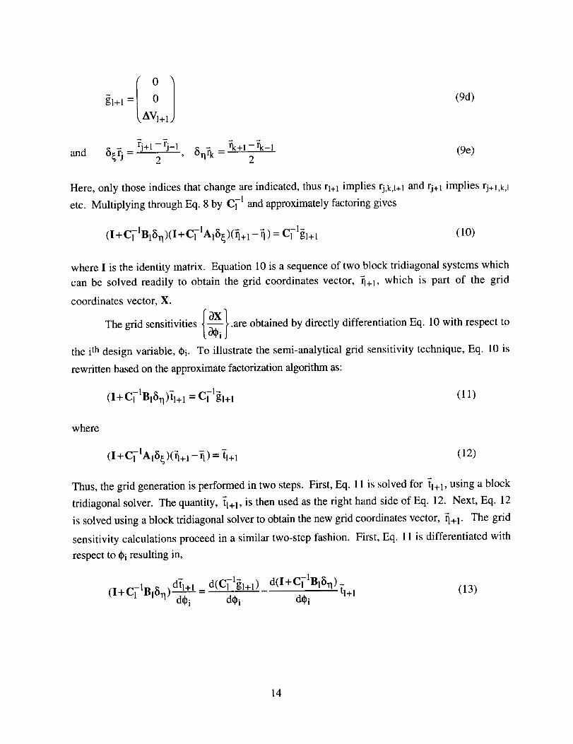
(9d)
and _j_ _+1-_-1 _1.1_k = rk+l -rk-1 (9e)2 ' 2
Here, only those indices that change are indicated, thus r1+1 implies rj,k,l+ 1 and rj+l implies rj+l,k, 1
etc. Multiplying through Eq. 8 by Ci -1 and approximately factoring gives
(I+ CIIBISrl)(I+Ci-IAlS_)(rl+l-rl) = ci-lgl+l (lO)
where I is the identity matrix. Equation 10 is a sequence of two block tridiagonal systems which
can be solved readily to obtain the grid coordinates vector, _1+1, which is part of the grid
coordinates vector, X.
The grid sensitivities { 0_ii }.are obtained bY directly differentiation Eq. 10 with respect t°
the ith design variable, 0i. To illustrate the semi-analytical grid sensitivity technique, Eq. 10 is
rewritten based on the approximate factorization algorithm as:
(I + Ci-lBl_in)tl+l = Cl-lgl+l (11)
where
(I +C1-1A18_)(_1+1 -_I)= tl+l (12)
Thus, the grid generation is performed in two steps. First, Eq. 11 is solved for tl+l, using a block
tridiagonal solver. The quantity, tl+l, is then used as the fight hand side of Eq. 12. Next, Eq. 12
is solved using a block tridiagonal solver to obtain the new grid coordinates vector, ?1+1. The grid
sensitivity calculations proceed in a similar two-step fashion. First, Eq. 11 is differentiated with
respect to g)i resulting in,
- d(ci-l_l+l) d(I+ci-lB18n)(I+CIIBIS_) d_ 1 =. tl+ 1
d_i d_iuwi
(13)
14
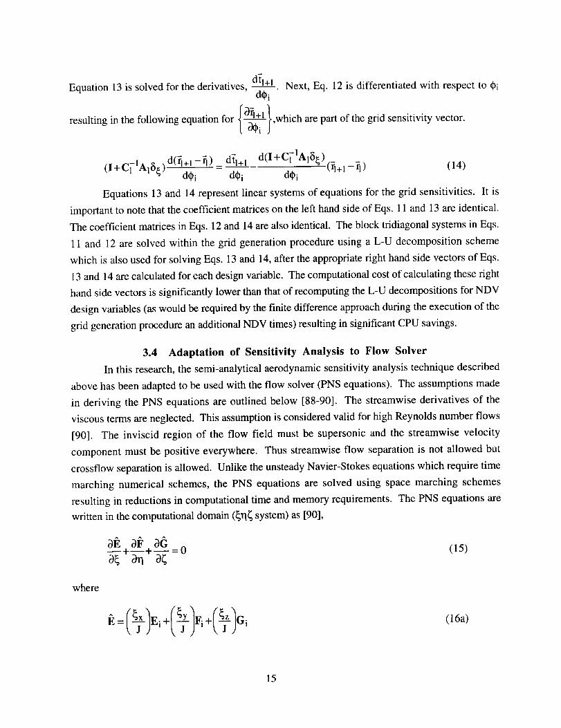
Equation 13 is solved for the derivatives, d_l+l Next, Eq. 12 is differentiated with respect to Oid_i
for {_t'which are part of the grid sensitivity vector.resulting in the following equation
(I+CIIAIS_) d(rl+l-rl) _ dt'l+l d(I+Cl-lAl_ )de i d0 i de i (rl+l -rl) (14)
Equations 13 and 14 represent linear systems of equations for the grid sensitivities. It is
important to note that the coefficient matrices on the left hand side of Eqs. 11 and 13 are identical.
The coefficient matrices in Eqs. 12 and 14 are also identical. The block tridiagonal systems in Eqs.
11 and 12 are solved within the grid generation procedure using a L-U decomposition scheme
which is also used for solving Eqs. 13 and 14, after the appropriate right hand side vectors of Eqs.
13 and 14 are calculated for each design variable. The computational cost of calculating these right
hand side vectors is significantly lower than that of recomputing the L-U decompositions for NDV
design variables (as would be required by the finite difference approach during the execution of the
grid generation procedure an additional NDV times) resulting in significant CPU savings.
3.4 Adaptation of Sensitivity Analysis to Flow Solver
In this research, the semi-analytical aerodynamic sensitivity analysis technique described
above has been adapted to be used with the flow solver (PNS equations). The assumptions made
in deriving the PNS equations are outlined below [88-90]. The streamwise derivatives of the
viscous terms are neglected. This assumption is considered valid for high Reynolds number flows
[90]. The inviscid region of the flow field must be supersonic and the streamwise velocity
component must be positive everywhere. Thus streamwise flow separation is not allowed but
crossflow separation is allowed. Unlike the unsteady Navier-Stokes equations which require time
marching numerical schemes, the PNS equations are solved using space marching schemes
resulting in reductions in computational time and memory requirements. The PNS equations are
written in the computational domain (_rl_ system) as [90],
(15)
where
E =/_j_)Ei + (_j_)Fi +/_j_/Gi(16a)
15

_'= (Ei-Ev)+ (Fi-Fv)+ -j-- (Gi-G v)(16b)
(16c)
The inviscid flux vectors (subscript i) and viscous flux vectors (subscript v) are defined by
Ei=[PUpu2+ppuv puw(Et+p)u]T
Fi=[PVpuvpv2+ppvw(Et+p)v]T
G,:[_wpuwpvwpw'+p (E_+p)w]_
(17)
E v =[0 l:xx "Cxy "_xz u'l:xx+V'l:xy +w'_xz-qx ]T
Fv=[0 _xy _yy _yz u'l:xy-I-V_yy-l-W'gyz-qy] T
Gv=[0 "_xz l:yz '_zz U'_xz+V'_yz+W'Czz-qz] T
(18)
(19)
The superscript "*" on the viscous flux vectors in Eqs. 16 indicates that derivatives with respect to
have been omitted. In these equations, p is the pressure, p is the density, u, v and w are the
velocity components in the x, y and z directions, respectively, e is the internal energy, x is the
viscous stress and q is the heat conduction rate. All physical quantities have been non-
dimensionalized appropriately [90]. The partial derivatives, _x, _y ..... _y, _z, are the metrics of
transformation between the _rl_ and the xyz system and J denotes the Jacobian of the
transformation. The flow solver is the UPS3D code [90] developed at NASA Ames Research
Center. The computational procedure used in this code integrates the PNS equations using an
implicit, approximately factored, finite-volume algorithm where the crossflow inviscid fluxes are
evaluated by Roe's flux-difference splitting scheme [91]. The UPS3D code also has the capability
of calculating the inviscid flow field, by solving the PNS equations without the viscous terms. In
the present research, this inviscid option has been used while evaluating the flow field. The
upwind algorithm is used to improve the resolution of the shock waves over that obtained with the
conventional central differencing schemes. The post-processor in the UPS3D solver evaluates the
non-dimensional force coefficients, such as lift coefficient (CL) and drag coefficient (CD), by
16
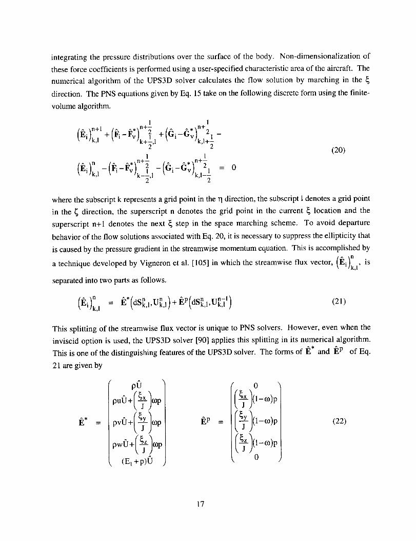
integratingthepressuredistributionsover the surfaceof the body. Non-dimensionalizationoftheseforcecoefficientsisperformedusingauser-specifiedcharacteristicareaof theaircraft. Thenumerical algorithm of the UPS3Dsolver calculatesthe flow solution by marching in the
direction.ThePNSequationsgivenbyEq. 15takeonthefollowingdiscreteform usingthefinite-
volumealgorithm.
1 1
(El ]n+l (Fi ^,.n+- ^,.n+- _,k.I + -FV)k+_, 1 + ((_i -GV)k,121
I 1
--n -Gv) 2 1 0- k,I, -_
(20)
where the subscript k represents a grid point in the 11 direction, the subscript I denotes a grid point
in the _ direction, the superscript n denotes the grid point in the current _ location and the
superscript n+l denotes the next _ step in the space marching scheme. To avoid departure
behavior of the flow solutions associated with Eq. 20, it is necessary to suppress the ellipticity that
is caused by the pressure gradient in the streamwise momentum equation. This is accomplished by
( )n isa technique developed by Vigneron et al. [105] in which the streamwise flux vector, ]_i k,l'
separated into two parts as follows.
i_ n , n(i)k,! = I_*(dS_,IUk,I)+I_P(dS_,I,U_I) (21)
This splitting of the streamwise flux vector is unique to PNS solvers. However, even when the
inviscid option is used, the UPS3D solver [90] applies this splitting in its numerical algorithm.
This is one of the distinguishing features of the UPS3D solver. The forms of 1_* and 1_p of Eq.
21 are given by
^
pU
^
(E t +p)U
EP
0
: o,p0
(22)
17

(23)
An eigenvalue analysis shows that Eq. 20 is hyperbolic-parabolic with respect to the new
dependent vector , provided that o_ satisfies the relation
(24)
where M_ is the Mach number in the _ direction and _ is a factor used to account for nonlinearities
^*( n n ) ,s evaluatednot otherwise included in the analysis. In Eq. 21, E dSk,l,Uk,! means that l_* "
from Eq. 22 using the values of the metrics and the flow variables corresponding to station n.
Similarly, the term I_p (dS_, I,U_A 1) in Eq. 21 indicates that 1_p is evaluated from Eq. 22 using the
values of the metrics corresponding to station n and the flow variables (including co) corresponding^_
to station (n-l). To avoid the difficulty of extracting the flow properties from the flux vector E
and to simplify the application of the implicit algorithm, a change is made in the dependent variable
from 1_* to the vector of conserved variables, U, using the following linearization.
where
U = [13 pu pv pw Et] T (26)
and
^,n-1 _1_* (dSn, Un-1 )
Ak, 1 = _un_ 1(27)
Using Roe's flux vector splitting for the crossflow fluxes, the Vigneron technique [105] for
suppressing departure solution and an implicit algorithm, Eq. 20 is approximately factored into two
block-tridiagonal systems to yield the following discrete governing equations for calculating the
flow field [88].
18
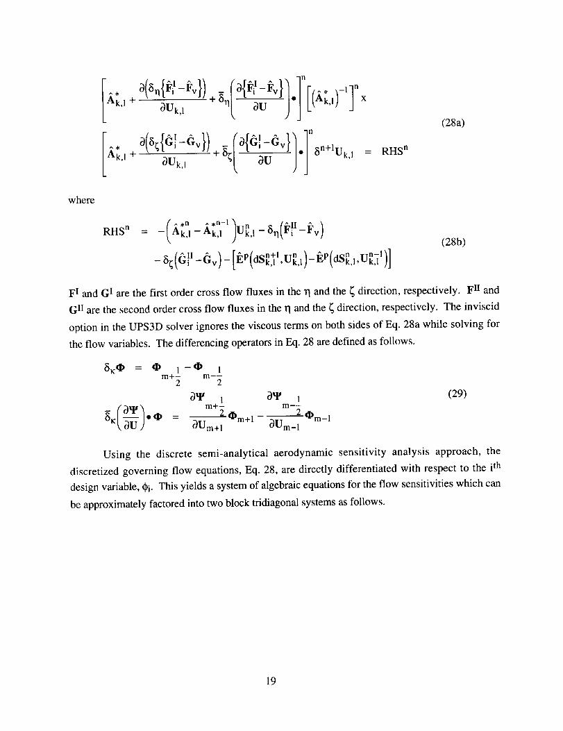
^, _ ,-,]°
^ ! ^ jnAk, I + _Uk, 1
= RHS n
(28a)
where
RHS n = - Ak, 1 -Ak, I Uk,I -Srl Fi
^ p n+l n ^ p n n-I
(28b)
F I and G I are the first order cross flow fluxes in the rl and the _ direction, respectively. F II and
G II are the second order cross flow fluxes in the rl and the _ direction, respectively. The inviscid
option in the UPS3D solver ignores the viscous terms on both sides of Eq. 28a while solving for
the flow variables. The differencing operators in Eq. 28 are defined as follows.
m+- m---2 2
_IJ 1 °_lIJ 1
m+_ 2 ¢I)m_l_ * _ -- OUm+ 1 I:][)m+l _Um_ 1
(29)
Using the discrete semi-analytical aerodynamic sensitivity analysis approach, the
discretized governing flow equations, Eq. 28, are directly differentiated with respect to the ith
design variable, ¢i. This yields a system of algebraic equations for the flow sensitivities which can
be approximately factored into two block tridiagonal systems as follows.
19

nA .,1+ onUk,l
],n
d¢i
k,l +
d
Ak, 1 +
()Uk,1
_ !iitI.F -F,, ^, ,,
ll> Ak, 1 X+ 8n OU
d_i
_n+l U k,1
(30)
It is to be noted that the block tridiagonal coefficient matrices on the left hand sides of Eqs. 28 and
30 are identical. Hence, the L-U decompositions of the block tridiagonal matrices of Eq. 28 can
also be used for the calculation of the flow variable sensitivities from Eq. 30. Thus, it is only
required to calculate the appropriate fight hand side vectors of Eq. 30 for all the design variables, in
order to calculate the flow variable sensitivities. In the finite difference approach, the flow solution
needs to be solved an additional NDV times which implies that the L-U decompositions of the
coefficient matrices of Eq. 28 are performed an additional NDV times. This makes the direct
differentiation approach computationally very efficient over the finite difference approach. The
following section describes the application of these procedures for the aerodynamic design
sensitivity analysis of a high speed wing-body configuration.
3.5 Design Sensitivity Calculations for Wing-Body Configurations
The semi-analytical sensitivity techniques for grid sensitivity and aerodynamic sensitivity
calculations, described above, are used to calculate the design sensitivities for a high speed
configuration. Numerical results for a delta wing-body configuration (Fig. 2) are presented here.
In this configuration, the center body is axisymmetric and is a combination of a nose region and an
extended cylindrical region. The forebody of the vehicle has a sharp nose with the radius, r,
varying quadratically with the axial coordinate, x, over the nose length, ln. The radius of the
2O

cylindrical region is denoted rm. The variation of the body radius of the body changes from the tip
to its maximum value, rm, over the nose length, In, is given by
r = rm-rm 1- (31)
Here, x is the axial coordinate measured from the tip of the aircraft. The wing planform parameters
include: leading edge sweep, )_, root chord, Co, wing span, Ws and the wing starting location, xw,
measured from the nose of the aircraft. The wing cross section is a diamond airfoil with the
thickness-to-chord ratio, tc. The total length of the body is denoted lb. The values of these
parameters used in the present case are: co = 7.08 m, )_ = 66.0 degrees, w s = 3.53 m, tc = 0.052,
rm = 0.57 m, In = 6.01 m, Xw = 8.21 m and lb = 17.52 m. A three-dimensional hyperbolic grid,
with 75 grid points in the circumferential (1"1) direction and 80 grid points in the normal (4)
direction, is generated around the wing-body configuration for the flow analysis using the UPS3D
solver. The space marching scheme of the UPS3D solver uses a step size of 0.01 m. The
aerodynamic sensitivities are calculated for a cruise Mach number of 2.5 and an angle of attack of 5
degrees.
The grid sensitivities with respect to the leading edge sweep 0_), root chord (Co), wing
span (Ws) and thickness-to-chord ratio (tc) are presented in Table 1. Comparisons are made with
those obtained using the finite difference technique. The finite difference grid sensitivities are
calculated by perturbing each of the four variables by 0.1 percent. As shown, there is excellent
agreement between the results from the two techniques. The sensitivities at the first grid point are
zero because this point lies in the nose region of the aircraft and the four variables considered are
all wing design variables which do not affect the grid in the nose region.
Grid point
(x, y, z)(0.300, 0.044,
O.O08)
(13.19,-0.561, 0.104)
Table 1. Grid sensitivity of the three-dimensional hyperbolic grid.
Design variable
Sweep (_,)
Root chord (c o)
Wing span (w s)
Thickness/chord (t c)
Sweep 0Q
Root chord (c o)
Wing span (w s)Thickness/chord (t c)
Finite difference grid
sensitivity method(0.000, 0.000, 0.000)
(0.000, 0.000, 0.000)
(0.000, 0.000, 0.000)
(0.000, 0.000, 0.000)
(0.0, 0.0016, 0.0001)
(0.0,-0.0171,-0.0109)
(0.0,-0.0148,-0.0096)
(0.0,- 1.0693,-0.7514)
Direct differentiation
_rid sensitivity method(0.000, 0.000, 0.000)
(0.000, 0.000, 0.000)
(0.000, 0.000, 0.000)
(0.000, 0.000, 0.000)(0.0, 0.0016, 0.0001)
(0.0,-0.0170,-0.0108)
(0.0,-0.0149,-0.0097)
(0.0,- 1.0695,-0.7517)
21

A comparisonof theCPUtime ona CRAY-2 [Fig.3] showsa40percentreductionachievedfor
one completegrid sensitivity analysisusingthe direct differentiation approachover the finitedifferencemethod.Thisclearlydemonstratesthesignificantcomputationalsavingsachievableby
using the direct differentiation approach. This is particularly important in a formal design
optimizationprocedurewhereseveralsuchdesignsensitivityanalysesarenecessary.
O
Fr
O"
ZO
0"Q
0
JWing span (ws)
9--
r_
v
J1
Section AA'
Figure 2. Delta wing-body configuration (schematic).
22

[] Finite difference
[] Direct differentiation
5OO
Figure 3.
tO
v
3OO
O
2O0
m
Comparison of CPU time (seconds) for the sensitivity of hyperbolic grid.
Results obtained from the aerodynamic sensitivity analysis procedure are presented next.
The sensitivities of the inviscid drag coefficient (CD) and the lift coefficient (CL), calculated using
the direct differentiation technique as well as the finite difference approach, are presented in Tables
2 and 3 respectively. It must be noted that column 3 in Tables 2 and 3 presents the results of the
semi-analytical aerodynamic sensitivity approach with finite difference grid sensitivity while
column 4 presents the results of the semi-analytical aerodynamic sensitivity approach with semi-
analytical grid sensitivity. As shown, the results from both techniques are in excellent agreement.
For one complete sensitivity analysis, the direct differentiation technique with finite difference grid
sensitivity calculations results in a 30.5 percent reduction in computing time compared to the fully
finite difference sensitivity analysis [Fig. 4]. The semi-analytical sensitivity analysis technique
with semi-analytical grid sensitivity calculations yields a 39 percent reduction in computing time
compared to the finite difference approach [Fig. 4]. This further illustrates the efficiency of the
discrete semi-analytical technique for grid sensitivity calculations.
23
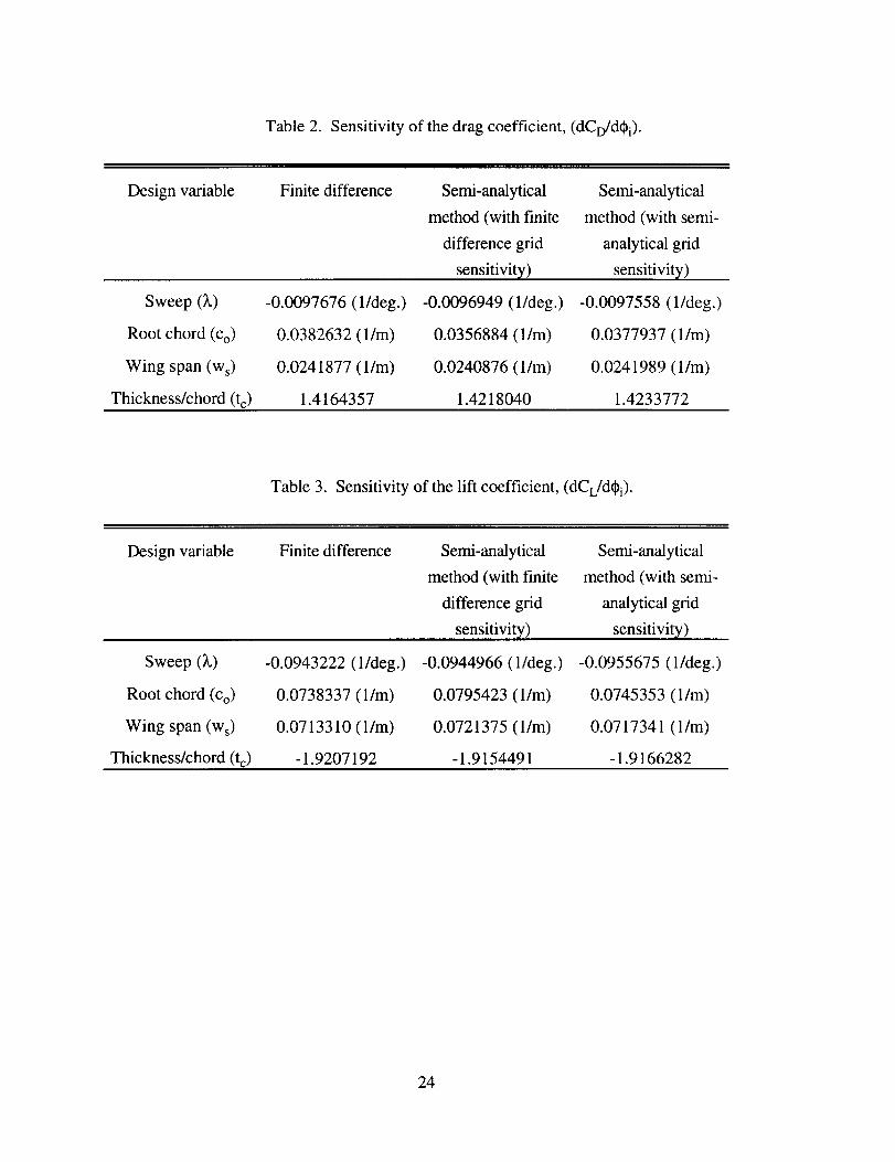
Table 2. Sensitivity of the drag coefficient, (dCD/dt_i).
Design variable
Sweep (_,)
Root chord (Co)
Wing span (Ws)
Thickness/chord (t c)
Finite difference
-0.0097676 (1/deg.)
0.0382632 (I/m)
0.0241877 (I/m)
1.4164357
Semi-analytical
method (with finite
difference grid
sensitivity)
-0.0096949 (1/deg.)
0.0356884 (I/m)
0.0240876 (I/m)
1.4218040
Semi-analytical
method (with semi-
analytical grid
sensitivity)
-0.0097558 (l/deg.)
0.0377937 (1/m)
0.0241989 (l/m)
1.4233772
Table 3. Sensitivity of the lift coefficient, (dCL/d¢i).
Design variable
Sweep (_,)
Root chord (Co)
Wing span (Ws)
Thickness/chord (tc)
Finite difference
-0.0943222 (1/deg.)
0.0738337 (I/m)
0.0713310 (l/m)
- 1.9207192
Semi-analytical
method (with finite
difference grid
sensitivity)
-0.0944966 (1/deg.)
0.0795423 (l/m)
0.0721375 (l/m)
- 1.9154491
Semi-analytical
method (with semi-
analytical grid
sensitivity)
-0.0955675 (1/deg.)
0.0745353 (I/m)
0.0717341 (I/m)
-1.9166282
24

[] Finite difference
[] Direct differentiation with finite difference grid sensitivity
[] Direct differentiation with semi-analyfcal grid sensitivity
/2000
1800
G"
'_ 1400
0
1200
1000
Figure 4.
"7
i°..°°.°°.°°°.°°.°,.°.. •
Comparison of CPU time for aerodynamic sensitivity analysis.
25

4. Optimization Techniques
The multidisciplinary optimization procedure for the design of aerospace systems such as
high speed wing-body configurations requires the integration of several major disciplines. Since
an "all-at-once" approach in such cases is complex and inefficient, the problem is formulated using
a non-hierarchical, multilevel decomposition technique. In general, the optimization problem at
each level involves several objective functions, constraints and design variables. In the present
work, two different multiobjective formulation techniques have been used. These are the
Kreisselmeier-Steinhauser (K-S) function [106-107] approach and the modified global criteria [ 13]
technique. At levels where the K-S function approach is used, the Broyden-Fletcher-Goldfarb-
Shanno (BFGS) algorithm [108] is used to solve the unconstrained nonlinear optimization
problem. At levels where a single objective function is involved, a nonlinear constrained
optimization algorithm based on the method of feasible directions [109-110] is used. At each level,
the optimization procedure is coupled with an approximate analysis technique based on a two-point
exponential expansion [111] thus making the overall procedure computationally efficient. The
following sections describe these procedures.
4.1 Multilevel Decomposition
The formulation of a MDO problem using a two-level procedure is illustrated in Fig. 5.
For example, in the case of an integrated aerodynamic and structural optimization of high speed
aircraft, level 1 may optimize aerodynamic criteria and level 2 may address structural criteria [92-
93, 100-101].
Each level is characterized by a multiobjective optimization problem with vectors of
objective functions, constraints and design variables. The formulation is outlined below.
Level 1
Minimize F_(tI _1) i = l, ..., NOBJ 1
subject to gl( t) _<0 k = l, --- , NC 1
NDVI _F2* 1
E "-_-il A_i
i=l
-< 82j J = I,...,NOBJ 2
,IL -<,I -- i = 1,... ,NDV l
26

NDV_1 2" _2U2* °-J*_...kJAA! _<,2L <_,j + ad
i=l
j = 1, ..., NDV 2
where F ! and F 2 are the objective function vectors at levels 1 and 2, respectively. The
corresponding constraint vectors are gl and g2 and the corresponding design variable vectors are
_1 and _2. The quantity E2 represents a tolerance on the changes to the jth objective function of
level 2, during level 1 optimization. Superscripts L and U refer to lower and upper bounds,
_F 2.
respectively and the superscript (*) represents optimum values. The quantities --_ are the
optimal sensitivity derivatives of the objective functions of level 2 with respect to the design
variables at level 1. The quantities _ represent the optimal sensitivity derivatives of the design
variables at level with respect to the design variables at level 1.
_2
Minimize F_(@I)
subject to gl(Ol) < 0
8t
_L
a,l ' a,
Minimize F2 (cl_l* ' t][_2 )
subject tog2 (till*, _[:)2) _<0
Level 1 (Aerodynamicsand/or sonic boom)
(Optimal sensitivity
parameters)
Level 2 (Structures)
Figure 5. Two-level decomposition (schematic).
Level 2
lVfirflrrflze F? (II:I I ,CI_2 ) i = 1, .-- , NOBJ 2
27

subject to g2k(_l ,_2)<0 k = 1,..-,NC 2
¢}2L _< 02 _< ,i2U i = 1,--.,NDV 2
where _1. is the optimum design variable vector from level 1. This vector is held fixed during
optimization at level 2. The optimization procedure cycles through the two-levels before global
convergence is achieved. A cycle is defined as one complete sweep through all the levels of
optimization. Optimization at an individual level also requires several iterations before local
convergence is achieved. The different levels are linked through the use of optimal sensitivity
parameters which are essential in maintaining proper interdisciplinary coupling.
4.2 Multiobjective Formulations
In general, a subproblem within a multilevel optimization procedure, as described above,
involves multiple objective functions and constraints. Since traditional optimization techniques
address problems with a single objective function, it is essential to use formal multiobjective
formulation techniques for such applications. In this research, two multiobjective formulation
techniques namely, the Kreisselmeier-Steinhauser (K-S) function approach and the modified global
criteria technique, have been used. The following sections describe these two formulations in
detail.
4.2.1 Kreisselmeier-Steinhauser (K-S) Function Approach
The Kreisselmeier-Steinhauser (K-S) function approach [ 106-107] has been successfully
used in various aircraft design applications [96-101]. In this approach, the original objective
functions are scaled into reduced objective functions. Depending on whether the individual
objective functions are to be minimized or maximized, these reduced objective functions assume
one of the two following forms
* Fk(_)
Fk(_) - Fko - 1.0 -gmax -< 0 k= 1..... NOBJmin (32a)
• Fk(O)
Fk(_) = 1.0- Fko -gmax -< 0, k = 1..... NOBJmax (32b)
where Fko represents the original value of the k th objective function (Fk) calculated at the beginning
of each cycle and • is the design variable vector, gmax represents the largest constraint in the
original constraint vector, gj(_), and is held constant during each cycle. The reduced objective
28
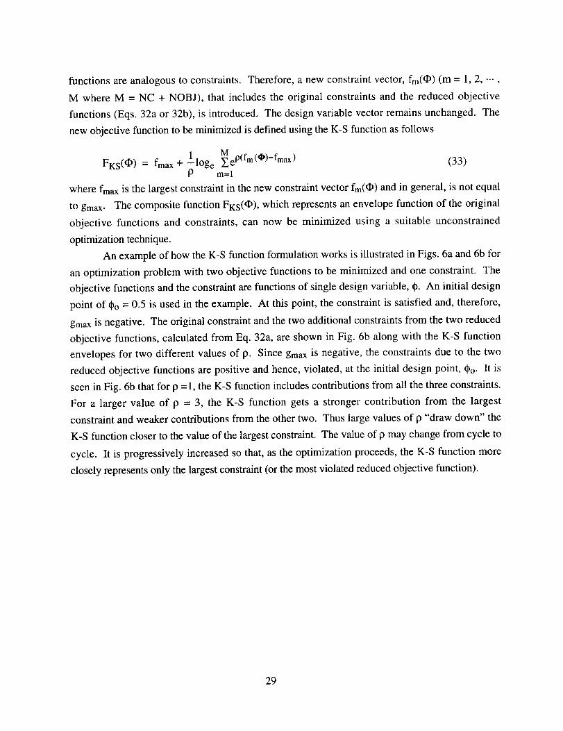
functionsareanalogousto constraints.Therefore,anewconstraintvector,fro(O) (m = 1,2, ...,
M where M = NC + NOBJ), that includesthe original constraintsandthe reducedobjective
functions(Eqs.32aor 32b), is introduced.Thedesignvariablevectorremainsunchanged.The
newobjectivefunctionto beminimizedis definedusingtheK-Sfunctionasfollows
MFKS(_) = fmax+ lloge Y_eP(fm(_)-frnax) (33)
P m=l
where fmax is the largest constraint in the new constraint vector fm(_) and in general, is not equal
to gmax. The composite function FKS(_), which represents an envelope function of the original
objective functions and constraints, can now be minimized using a suitable unconstrained
optimization technique.
An example of how the K-S function formulation works is illustrated in Figs. 6a and 6b for
an optimization problem with two objective functions to be minimized and one constraint. The
objective functions and the constraint are functions of single design variable, _. An initial design
point of _o = 0.5 is used in the example. At this point, the constraint is satisfied and, therefore,
gmax is negative. The original constraint and the two additional constraints from the two reduced
objective functions, calculated from Eq. 32a, are shown in Fig. 6b along with the K-S function
envelopes for two different values of p. Since gmax is negative, the constraints due to the two
reduced objective functions are positive and hence, violated, at the initial design point, _o. It is
seen in Fig. 6b that for p = 1, the K-S function includes contributions from all the three constraints.
For a larger value of p = 3, the K-S function gets a stronger contribution from the largest
constraint and weaker contributions from the other two. Thus large values of p "draw down" the
K-S function closer to the value of the largest constraint. The value of p may change from cycle to
cycle. It is progressively increased so that, as the optimization proceeds, the K-S function more
closely represents only the largest constraint (or the most violated reduced objective function).
29
objective objective
function 1 function 2
0
-0.51
-1 !
\
I I I I I
0.2 0.4 0.6 0.8 1
Design variable,
Figure 6a. Original objective functions and constraints.
F 1 - reduced objective function 1
F 2 - reduced objective function 2
gl - constraint 1
KS (p = 1) KS (p = 3)
-1
F 2
g
0 0.2 0.4 0.6 0.8 1
Design variable, 0
Figure 6b. K-S function envelope.
F !
4.2.2 Modified Global Criteria Approach
The modified global criteria approach [13] is an alternate way to formulate multiobjective
problems. In order to understand this approach, consider a problem with two objective functions,
fl (O) and f2(_). Let r1 and f2 be their corresponding individually optimized values or known
30
target values. The two original objective functions are combined into the global criteria function,
F(_), as follows.
F(cI_) = 4(fl - fi) 2 + (f2 - f2) 2 (34)
The global criteria function, F(_), represents the new objective function which is to be minimized.
The minimization of F(_) forces the values of fl and f2 towards their target values.
4.3 Approximate Analysis
The optimization techniques used in this research are gradient-based and they require
evaluations of the objective functions and constraints during every iteration of optimization. Since
it is computationally expensive to evaluate these functions through exact analysis all the time, an
approximate analysis technique is used within each iteration of the optimization. The two-point
exponential approximation technique developed by Fadel et al. [111], has been found to be well
suited for nonlinear optimization problems and has been used in the present research for
approximating the objective functions and the constraints within the optimizer. The technique is
formulated as follows.
N°vI/0nlpnl_(*) = F(*I)+ n__.__1 _ -1.0 Pn c_bn(,z,l) (35)
where l_k(CI_) is the approximation to the objective function Fk at a neighbouring design point _,
based on its values and its gradients at the current design point _l and the previous design point
_0. The approximate values for the constraints, _j(q_), are calculated in a similar fashion. The
exponent Pn, in Eq. 35 is defined as:
Pn = + 1.0 (36)l°ge{_On } - l°ge{_ln }
The exponent Pn explicitly determines the trade-offs between traditional and reciprocal Taylor
series based expansions (also known as a hybrid approximation technique). In the limiting case
when Pn = 1, the expansion is identical to the first order Taylor series and when Pn = -1, the two-
point exponential approximation reduces to the reciprocal expansion form. In the present work,
the exponent is defined to lie within this interval, - 1 < Pn < 1. If the exponent Pn is greater than 1,
it is set equal to one and if Pn is less -1, it is set equal to -1. Equations 35 and 36 indicate that
31

many singularity points may exist in the use of this method and hence, care must be taken to avoid
such points. In the present study, when singularity problems arise, the approximation technique is
reduced to the linear Taylor series expansion (Pn = 1).
5. Applications of Multidisciplinary Design Optimization
A significant aspect of this research has been the development and application of MDO
procedures for aerospace designs. Several different MDO procedures have been developed. The
first example optimizes a theoretical, minimum drag body of revolution. This procedure is similar
to the optimization study conducted by Cheung et al. [78] and serves as a benchmark test for the
optimizer. The second example addresses the integrated aerodynamic/structural optimization of
high speed, delta wing-body configurations. The two-level decomposition technique described
earlier has been used in this application. The third MDO procedure has been used for the coupled
aerodynamic and sonic boom optimization of high speed wing-body configurations in a single
level. The K-S function multiobjective formulation technique is employed within this application.
The fourth MDO procedure has been developed using a two-level decomposition technique for
high speed wing-body design where aerodynamic and sonic boom criteria are improved in level 1
and structural criteria are optimized in level 2. These four MDO procedures use the
computationally intensive CFD solver, UPS3D [90], for aerodynamic analysis. Hence, the semi-
analytical sensitivity analysis techniques for calculating aerodynamic design sensitivities are used
for these four MDO procedures.
5.1 Aerodynamic Optimization of a Theoretical Minimum Drag Body
The first optimization procedure is applied to a body of revolution to minimize its wave
drag. The reference geometry used is the Haack-Adam (H-A) body [117-118]. This is a body of
revolution with a pointed nose and a base of finite area (Fig. 7). The H-A body has minimum drag
amongst all bodies in its class, according to slender-body theory for linearized, supersonic flows
[117-118]. In the present research, the minimization of the wave drag coefficient (inviscid, no lift
case) of the H-A body is carried out as a benchmark test. Results obtained are compared with
those obtained in Ref. 78.
5.1.1 Haack-Adam (H-A) Body
The H-A body (Fig. 7) is an axisymmetric body whose radius, r, varies with the axial
coordinate, x, as follows.
32

r 2 Abase 7t-0+ sin20 +714sin30+ ]_ ]t m2 XAma x 3 m=2 _ m m+2rmax
(43)
where
(44)
In the above equations, Abase is the base area of the H-A body, Amax is the cross-sectional area at
the section of maximum thickness (Xmax) and lb denotes the length of the body. The wave drag is
non-dimensionalized by the product of the freestream dynamic pressure and the maximum cross-
sectional area (Amax). The resulting wave drag coefficient (CDw), from slender body theory, is
given by
_g
.,.,_
I I I I I I I I I
0. l 0.2 0.3 0.4 0.5 0.6 0.7 0.8 0.9
Axial coordinate, x (m)
Figure 7. Haack-Adam body.
71;12 I(4Abase/2 '' +l)(4A___b_se ]tm/2 }CDw-4 maxkt (m t,(45)
By definition, a H-A body satisfies the conditions that 1) the base area, Abase, is fixed and non-
zero, 2) the slope at the end, (dA/dx)lx=lb , is zero and 3) the location of the maximum thickness,
Xmax, is fixed. It can be verified that Eq. 43 satisfies the first two conditions automatically. The
third condition determines the value of _'1 to be,
1 _ 1b (46)_t1 - 2cOS0max 2(2Xmax-lb)
33
Thewavedragcoefficientis independentof thefreestreamMachnumberbecausetheH-A bodysatisfiestheconditionthattheslopeof theareaattheend,(dA/dx)lx=ib, is zero. FromEq. 45, it is
clearthat,for abodywith minimumwavedrag,_'m= 0 for m > 2.
5.1.2 Results and Discussion
In the present research, the optimization of the H-A body is initiated with identical
geometric parameters as reported in Ref. 78. The length of the H-A body (lb) = 0.9 m and the
fineness ratio (lb/2rmax) = 7. The location of the maximum thickness (Xmax) = 0.525 m and the
corresponding value of theta (emax) = cos -1(1/6). The ratio of the base area to the maximum area
(Abase/Amax) = 0.532. Condition 3 requires the H-A body to satisfy (dA/dx)lx=Xmax = 0. In the
present research, this slope has been allowed to change in such a way that -1 < (dA/dx)lx=Xmax _<1.
This condition is expressed as follows.
2sin 0ma x +471 sin 2 0ma x cOS0max +
]_ )'m {c°s(m)0max - cos(m + 2)0ma x }m=2
< 1 (47)
Also, a constraint is imposed during the optimization to ensure that the radius of the optimal body
is greater than zero. This constraint is expressed as follows.
(re-0 +2sin 20)+ )'1 4sin3 0+ m=2_" "fm (sin(m)0'-m sin(m +2)0m+2 j>0(48)
for all rt > 0 > 0.
In the present research, five coefficients from Eq. 43, namely, )'2, "f3..... _'6 have been
used as design variables. The reference values of these five coefficients are zeroes, corresponding
to the theoretical minimum wave drag H-A body (Eq. 45). The wave drag coefficient (CDw) is
used as the objective function to be minimized subject to two constraints, given by Eqs. 47 and 48.
The optimization is carried out at a free stream Mach number of 2.5 and angle of attack of zero
degrees. The flow analysis is performed using the UPS3D solver [90-91] and the inviscid option
has been used to obtain the wave drag coefficient. The computational grid uses 21 points in the
circumferential (rl) direction, 70 points in the normal (_) direction and a maximum marching step
size of 0.0009 m. Table 4 presents the reference and optimum values of the design variables and
the wave drag coefficient. In Table 4, column 2 reproduces the optimum values obtained by
Cheung et al. [78] and column 3 gives the optimum values obtained from the present research.
The developed procedure yields a 6.6 percent reduction in the wave drag coefficient which is better
34
thanthe5 percentreductionachievedin Ref. 78. Figure8 comparesthedragcoefficientsof thereferenceandtheoptimumconfigurations.Clearly, thecurrentprocedureyieldsa betteroptimum
thanthatobtainedin Ref.78. Figure9 comparesthereferenceandoptimumconfigurations.The
optimum body hasa reducedradiusdistribution in the noseregioncomparedto the referencegeometry,in orderto reducethewavedragcoefficient. However,theradiusof theaft increasesin
theoptimumconfigurationin orderto satisfythetwo constraintsimposedduring theoptimization
(Eqs.47and48). Similar trendsareobservedin theoptimumgeometryobtainedin Ref.78.
Table4. Comparisonof designvariablesandobjectivefunction.
Designvariablesand
performancefunction
Reference(Haack- Optimum Optimum
Adambody) (Cheun_) (present)0.00000 0.85300 0.73866
0.00000 0.67300 0.45117
0.00000 0.49500 0.276020.00000 0.42000 0.38728
0.00000 0.08460 0.15854
0.07599 0.07220(-5.0 %) 0.07095(-6.6 %)
¥2
Y3
Y4
Y5
Y6
Dra_coefficient,CD
0.08-!
[] reference (Haack-Adam)
[] optimum (Cheung)
[] optimum (present)
0.076- /
-5.0 % -6.6 %0.072-
O
¢.J
_O 0.068-
: 0.064-
0.06 /-
Figure 8. Comparison of wave drag coefficient (CDw)-
35

i m
reference
...... optimum (Cheung)
0.07 - _ optimum (present)
0.05- ,, " " ,, ,, ,, " " _ " " ""
0.03
0.01-0.01
-0.03
-0.05
-0.07 i i i i i i i0 0.1 0.2 0.3 0.4 0.5 0.6 0.7 0.8 0.9
Axial coordinate, x (m)
Figure 9. Comparison of reference and optimum body configurations.
5.2 Multidisciplinary Optimization of High Speed Wing-Body Configurations
The second MDO procedure developed in this research uses a two-level decomposition
technique that addresses the simultaneous improvement of aerodynamic and structural performance
of high speed wing-body configurations [92-93]. From aerodynamics point of view, the drag
coefficient (CD) must be minimized while maintaining the lift coefficient (CL) above a desired
value. From a structural perspective, the aircraft weight (W) must be minimized while maintaining
the stresses in the load carrying members within allowable limits. These requirements are
formulated as a two-level optimization problem as follows.
5.2.1 Multilevel Optimization Formulation
In a typical aircraft design, the aerodynamic performance criteria dictate the planform
geometry of the aircraft wing. After designing the planform, the wing load carrying member is
designed to carry the loads arising from aerodynamics, inertia and gravity. Keeping this in mind,
the two-level optimization procedure improves the wing-body aerodynamic performance at level 1
and the structural performance at level 2. These optimization problems are stated as follows.
36

Level 1 (Aerodynamics)
Mmirrflze
Drag coefficient (CD)
subject to the constraints
CL -> CLmin (Lift coefficient constraint)
W<W* (Optimal weight constraint)
L * NDVI _0J2A u_bj2 -< _bj2 + _ _il -< _j2
i= 1 _Oil j = 1..NDV2 (Side constraints)
L U
_il -< (_il -< (_il i = 1..NDV1 (Side constraints)
where _l denotes the vector of aerodynamic design variables, _2 denotes the structural design
variable vector, NDVl and NDV2 denote the number of aerodynamic and structural design
variables respectively and the superscripts L and U denote lower and upper bounds on the design
variables respectively.
Level 2 (Structures)
Miffmflze
Weight (W)
subject to the constraints
(Y --< (Yall (Stress constraints)
L U
(_i2 <- (_i2 -< t_i2 i= 1..NOV2 (Side constraints)
where a is the vector of stresses at aircraft wing root and (Sall is the corresponding vector of
material limits. During the structural optimization at the second level, the aerodynamic design
variables of level 1 (¢1) are held fixed at their optimum values. The quantities, _)W* ¢)t_j20t_il and-_i 1 are
the sensitivities of the optimum values of the second level (structural) objective function and the
37

design variables with respect to first level (aerodynamic) design variables. These optimal
sensitivity derivatives provide the necessary coupling between the two disciplines.
5.2.2 Wing-Body Configuration
The two-level procedure and the semi-analytical sensitivity analysis techniques are applied
to the design optimization of the delta wing-body configuration illustrated in Fig. 2. The
description of the delta wing-body configuration has been presented earlier. The values of the
parameters describing the delta wing-body configuration are: wing root chord (Co) = 7.08 m,
leading edge sweep (_) = 66.0 degrees, wing span (Ws) = 3.53 m, wing thickness-to-chord ratio
(tc) = 0.052, maximum radius (rm) = 0.57 m, nose length (ln) = 6.01 m, wing starting location
(Xw) = 8.21 m and body length (lb) = 17.52 m. This reference design has been used in Ref. 120
for sonic boom prediction and comparison with wind-tunnel data. The wing leading edge sweep
0_), root chord (Co), wing span (Ws) and thickness-to-chord ratio (tc) are used as design variables
in level 1 optimization and hence, change from their reference values during optimization. The rest
of the planform parameters of the delta wing-body are held fixed throughout the optimization.
5.2.3 Wing Structural Model
In this study, a simple structural model has been used. The wing is assumed to carry all
the aerodynamic loading. The load carrying structural member of the wing is modeled as a single
celled, isotropic, rectangular box beam with unequal wall thicknesses [Fig. 10]. In Fig. 10, the
quantity c is the local chord length of the wing section. The beam width-to-chord ratio (Wc),
horizontal wall thickness-to-chord ratio (tw) the vertical wall thickness-to-chord ratio (tv) are used
as design variables during the structural optimization at level 2.
The wing structural analysis is performed using a code developed in-house. The code is
capable of analyzing single celled isotropic box beams with rectangular cross-sections, unequal
horizontal and vertical wall thicknesses and linear sweep and taper distributions. The structural
analysis is initiated slightly inwards of the wing tip. This ensures that the sharp wing tip of the
delta wing-body does not give rise to a singular point. The wing weight (W) is calculated as the
sum of the weight of the box beam (Wbox) and the weight of the skin (Wskin). The normal and
shear stresses 03) at the root section of the beam are calculated using thin wall theory [119]. The
isotropic box beam and the wing skin are made of 2014-T6 Aluminum alloy. The alloy has a
density of 2800 Kg/m 3, tensile yield strength of 410 MPa and a shear yield strength of 220 MPa.
The reference values of structural design variables are: spar width-to-chord ratio (Wc) of 0.5, spar
horizontal wall thickness-to-chord ratio (tw) of 0.0015 and vertical wall thickness-to-chord ratio
(th) of 0.0075.
38
k Wc*C --_
Diamond airfoilWing spar
tv*C
__7,,/I
L.... /____I
tw*CWing spar (Box beam)
Figure 10. Wing cross-section and wing spar (box beam).
5.2.4 Results and Discussion
The optimization is performed for a cruise design Mach number of 2.5 and an angle of
attack of 5 degrees. The inviscid, supersonic flow field is calculated using the CFD solver,
UPS3D [90]. The inviscid drag and the lift forces are non-dimensionalized using the product of
the dynamic pressure and a unit reference area, to yield a drag coefficient, denoted CDu, and a lift
coefficient, denoted CLu. Though the use of a unit reference area yields high values for these non-
dimensional coefficients, improvements in these coefficients directly reflect improvements in the
corresponding aerodynamic forces. A maximum step size of 0.01 m is used to march in the
direction. The aerodynamic design sensitivities, required during the level 1 aerodynamic
optimization, are calculated using the semi-analytical sensitivity analysis procedures [94-95]
described before. A hyperbolic grid with 75 points in the circumferential (11) direction and 80
points in the normal (_) direction is used for the flow analysis. Further refinement of the grid does
not alter the flow solution.
The iteration histories of the drag and the lift coefficients (CDu and CLu) of the wing-body
configuration, during the level 1 aerodynamic optimization, are compared in Figs. 11 and 12,
respectively. Significant improvements are observed in both the quantities. The drag coefficient
decreases by 5.5 percent and the lift coefficient increases by 5.43 percent. All the increase in the
lift coefficient occurs in the first iteration of the optimization after which the lift coefficient is
maintained at its improved value through the rest of the optimization. The lift coefficient constraint
39

is a violated constraint in the first cycle of optimization. The optimizer, based on the method of
feasible directions, establishes feasibility by increasing the lift coefficient to its desired value,
CLmin, in the first cycle. Increasing the lift coefficient any further results in an associated increase
in the induced drag. As a result, the optimizer maintains the lift coefficient constraint active. The
constraint imposed on the weight, is well satisfied during the level 1 optimization.
0.26"
_ 0.25
0.24
0 I0 20 30
Iteration
Figure 11. Iteration history of drag coefficient, (CDu).
Figure 12.
2.45 -
,5
_ 2.4o.
"_ 2.35 "
2.30"
2.25 • , , •
I O 20 30 40
Iteration
Iteration history of lift coefficient, (CLu).
Table 5. Aerodynamic design variables.
Design variable Reference Optimum
Sweep (_,) 66.00 deg. 65.33 deg.
Root Chord (c o) 7.08 m 7.70 m
Wing Span (Ws) 3.530 m 3.617 m
Thickness-to-chord (tc) 0.05200 0.03105
Table 5 compares the reference and the optimum values of the aerodynamic design variables used
in the aerodynamic optimization. The root chord is increased significantly from its reference value
40

(8.76 percent), whereas the wing thickness-to-chord ratio is decreased significantly (40.29
percent). The wing span and the leading edge sweep are maintained close to their reference values
(2.94 percent and 1.01 percent respectively). The reduction in the wing thickness-to-chord ratio
decreases the form drag of the diamond airfoil section. The optimization is driven by this reduction
in drag. The increase in the wing planform area, caused by the increase in the root chord and the
wing span, helps improve the lift of the aircraft in spite of the decrease in the wing thickness-to-
chord ratio. Though the drag and the lift coefficients have been non-dimensionalized using a unit
reference area in this study, the optimization procedure allows a traditional non-dimensionalization
using the wing planform areas.
The iteration history of the weight of the wing body configuration is presented in Fig. 13.
Considerable reduction (18.13 percent) in the weight is observed. The shear and the normal
stresses at the blade root remain well within the allowable limits of the chosen Aluminum alloy.
Table 6 compares the reference and optimum values of the structural design variables. The spar
width to chord ratio, horizontal and vertical wall thickness to chord ratios decrease significantly
from their reference values (60 percent, 60 percent and 65.2 percent respectively). In spite of the
increased planform area, the weight is reduced through significant reductions to the wall
thicknesses and wing thickness-to-chord ratio.
Weight(Kg)
33000
32000
31000
30000
29000
28000
27000
26000
0 10 20 30 40 50 60
Iteration
Figure 13. Iteration history of weight.
41
Table 6. Structural design variables.
Design variable
Spar width-to-chord ratio (Wc)
Horizontal wall thickness-to-chord ratio (tw)
Vertical wall thickness-to-chord ratio (tv)
Reference Optimum
0.5 0.2
0.0015 0.0006
0.0075 0.00261
5.3 Integrated Aerodynamic/Sonic Boom Optimization
One of the desired objectives of high speed (supersonic) aircraft designs is to arrive at low
sonic boom configurations. Such designs would have minimum environmental impact thus
making them viable for operation over population centers. At the same time, such designs should
also be able to produce optimum aerodynamic performance so that they are economically viable
too. These considerations give rise to an important multidisciplinary design optimization problem
requiring minimum sonic boom and maximum aerodynamic performance from the designs. In this
section, an optimization procedure that has been developed to reduce the sonic boom levels of high
speed wing-body configurations without deteriorating their aerodynamic performance, is
described. The sonic boom of an aircraft is measured in terms of the pressure disturbances it
produces at designated distances from the aircraft. The pressure disturbance at any point is given
by Ap = (p - poo)/po,,, where p is the pressure at the point of interest and poo is the free stream
pressure. Figure 14 presents the overpressure signature (Ap) produced by the delta wing-body
configuration described in Section 3.5. The aircraft is flying at a Mach number of 2.5 and angle of
attack of 5 degrees at a cruise altitude of about 16,500 m. The pressure signature is captured at the
ground level (this corresponds to 941.2 times the length of the aircraft, vertically below the
aircraft). The pressure signature has two positive pressure peaks and a negative peak. The first
positive pressure peak (Apl) corresponds to the pressure jump associated with the shock wave at
the nose of the aircraft. The second positive peak (Ap2) is due to the shock wave created by the
aircraft wing. The negative pressure peak corresponds to expansion waves in the flow field past
the wing trailing edge. From a sonic boom perspective, it is desirable to minimize these positive
pressure peaks in the overpressure signal. From aerodynamics point of view, it is of interest to
minimize the aerodynamic drag to lift ratio (CD/CL) while maintaining the lift coefficient (CL) at a
desired level. In the following sections, the sonic boom analysis procedure and the various
optimization formulations to reduce sonic boom levels of high speed wing-body configurations are
presented.
42

Figure 14.
0.003 -
0.002 -
0.001o'J
E_¢_ 0©
-0.001
-0.002
7150
AP 2
I I I I
7200 7250 7300 7350
x (m)
Sonic boom pressure signature of a supersonic wing-body configuration.
5.3.1 Sonic Boom Analysis
For isentropic flow past smooth axisymmetric bodies, the pressure disturbances (sonic
boom) at large distances from the aircraft can be evaluated by using the Whitham F-function [121 ],
which is based on the Abel integral of the equivalent area distribution of the aircraft. Lighthill
[122] developed an alternate formulation of the F-function which was shown to be suitable for
sonic boom prediction for projectile geometries. Walkden [123] extended Whitham's theory for
application to wing-body configurations. The asymptotic forms of the equations used in
developing the sonic boom overpressure signature (Ap) are as follows.
F(y) = _- 13Rvol (t)
I2h1 oo [_RI+2-_ _ft(t)
i
y-t dSvol(t)
13Rvol (t)
i
y-t dSlift(t )13Rl ft(t)
I 2 hi y-t ]dS,int(t)+ 1 i _R_nt(t) L[3Rint(t)
Ap = yM_F(y)/
= (Moo 2 - 1) 0.5
_: = (T + 1)Moo4/[_*(2_) 0'5]
(49)
(5O)
(51)
(52)
43

x = y+13do-_c.fd--_oF(y) (53)
where y is the ratio of specific heats (1.4 for air) and Moo is the freestream Mach number. The first
integral of Eq. 49 is associated with the volume of the flying object, the second integral is
associated with the lift and the third integral is associated with the interference lift for a winged
body [123]. Rvol, Rlift and Rint are the equivalent radii of the flying object based on its volume,
lift and wing-body interference, S' is the derivative of the area distribution of the flying object and
h is the Heaviside unit step function. The quantity, y(x, do) = constant is a characteristic curve
where x is the streamwise distance and do is the distance normal to the flight axis. Since the above
models are based on linearized theory, they are inaccurate in predicting sonic boom in highly
nonlinear flows such as the flow at angle-of-attack at higher Mach numbers (Moo > 2). Reference
124 describes an F-function extrapolation method to evaluate the pressure signature at a distance d l
from known pressure at distance do (dl > do). The pressure signature at distance do, where the
flowfield is assumed to be locally axisymmetric, is evaluated either by measurements in a wind
tunnel or through computation and the value of the F-function is calculated from Eq. 50. Since the
pressure signal propagates at the local speed of sound and each point of the signal advances
according to its amplitude, the signal is distorted and the F-function becomes multivalued at a
farther distance dr. A new F-function at dl is then obtained by placing discontinuities (shocks) in
such a way that the discontinuities divide the multivalued regions with equal areas on either side of
them. This new F-function gives the overpressure signature at dl using Eqs. 50 through 53.
Cheung et al. [120] have combined Whitham's quasilinear theory with the three-
dimensional PNS code, UPS3D, to predict sonic boom. The flow field associated with wing-body
configurations is evaluated by UPS3D and the overpressure signal for the near field is evaluated.
The overpressure signals at specified far fields are then obtained using one of three different
approaches for various configurations such as a cone-cylinder, a low aspect-ratio rectangular wing
and a delta wing-body. In the first approach (for nonlifting cases), the UPS3D code is modified so
as to incorporate a sonic boom prediction capability including all nonlinear effects. The second
approach is applicable to both lifting and nonlifting cases. In this approach, the extrapolation
method described earlier [ 124] has been used for predicting sonic boom. In the third approach (for
lifting cases), the equivalent area distribution due to lift is generated by the surface pressure
coefficients calculated by the CFD solver. The equivalent area distribution due to volume is
calculated from the geometry of the aircraft. Summation of the two equivalent area distributions
yields the total equivalent area distribution that gives the F-function of the body.
44

In thepresentresearch,thesecondapproach,basedontheextrapolationtechniqueof Ref.124,hasbeenusedto obtainthesonicboomsignatures.Thisextrapolationprocedurehasbeen
validatedby comparisonwith windtunneldatain Ref. 120by applyingit to thedeltawing-body
configurationdescribedin Section3.5.
5.3.2 Sonic Boom Sensitivities
The optimization procedures used for sonic boom minimization require the sensitivities of
the overpressure peaks (Apl and Ap2). The near field pressure signature, at a distance do, is
directly calculated by the UPS3D code. The sensitivity of this near field pressure signature is part
of the aerodynamic flow sensitivities calculated using the semi-analytical procedure based on the
direct differentiation approach [94-95], described earlier. Using these sensitivities, perturbed near
field pressure signatures are generated for each design variable. These perturbed near field
signatures are then extrapolated using the sonic boom extrapolation procedure [124] to obtain
perturbed far field signatures corresponding to each design variable. These perturbed far field
signatures are then used to obtain the sensitivities of the pressure peaks using finite difference
techniques.
5.3.3 Optimization Formulation
The multidisciplinary optimization procedure must lead to minimum sonic boom while
maintaining or improving the aerodynamic performance of the aircraft. From a sonic boom
perspective, it is desirable to minimize the first and the second peaks (Apl and Ap2) in the
overpressure signal at a given distance, dn, away from the aircraft. From aerodynamics point of
view, the drag to lift ratio (CD/CL) must be minimized while maintaining the lift coefficient (CL) at a
desired level. The optimization problem can be stated as follows.
Minimize
Apl, Ap2 and CD/CL
subject to the constraints
CLmin <- CL -< CLmax
CI_min < cI_ _< Cl_max
where • is the design variable vector and the subscripts "min" and "max" denote lower and upper
bounds, respectively. It must be noted that both upper and lower bounds have been imposed on
45
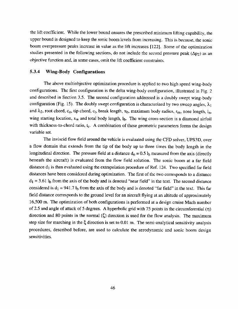
the lift coefficient. While thelowerboundensurestheprescribedminimumlifting capability,theupperboundis designedto keepthesonicboomlevelsfrom increasing.This isbecause,thesonic
boomoverpressurepeaksincreasein value as the lift increases [122]. Some of the optimization
studies presented in the following sections, do not include the second pressure peak (Ap2) as an
objective function and, in some cases, omit the lift coefficient constraints.
5.3.4 Wing-Body Configurations
The above multiobjective optimization procedure is applied to two high speed wing-body
configurations. The first configuration is the delta wing-body configuration, illustrated in Fig. 2
and described in Section 3.5. The second configuration addressed is a doubly swept wing-body
configuration (Fig. 15). The doubly swept configuration is characterized by two sweep angles, XI
and )_2, root chord, Co, tip chord, ct, break length, Xb, maximum body radius, rm, nose length, ln,
wing starting location, Xw and total body length, lb. The wing cross-section is a diamond airfoil
with thickness-to-chord ratio, tc. A combination of these geometric parameters forms the design
variable set.
The inviscid flow field around the vehicle is evaluated using the CFD solver, UPS3D, over
a flow domain that extends from the tip of the body up to three times the body length in the
longitudinal direction. The pressure field at a distance do - 0.5 lb measured from the axis (directly
beneath the aircraft) is evaluated from the flow field solution. The sonic boom at a far field
distance dj is then evaluated using the extrapolation procedure of Ref. 124. Two specified far field
distances have been considered during optimization. The first of the two corresponds to a distance
dl = 3.61 lb from the axis of the body and is denoted "near field" in the text. The second distance
considered is dl- 941.7 lb from the axis of the body and is denoted "far field" in the text. This far
field distance corresponds to the ground level for an aircraft flying at an altitude of approximately
16,500 m. The optimization of both configurations is performed at a design cruise Mach number
of 2.5 and angle of attack of 5 degrees. A hyperbolic grid with 75 points in the circumferential (q)
direction and 80 points in the normal (_) direction is used for the flow analysis. The maximum
step size for marching in the _ direction is set to 0.01 m. The semi-analytical sensitivity analysis
procedures, described before, are used to calculate the aerodynamic and sonic boom design
sensitivities.
46
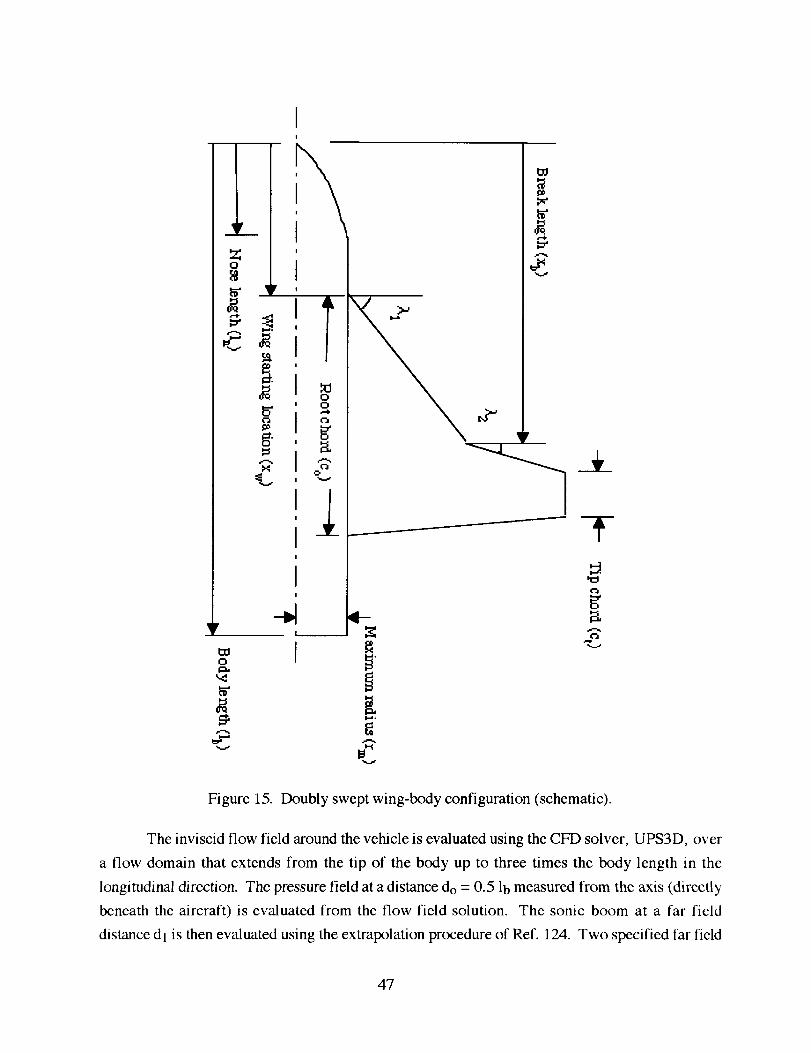
Oi:a,
II-i°
V
_0
...-.%
V
V
Figure 15. Doubly swept wing-body configuration (schematic).
The inviscid flow field around the vehicle is evaluated using the CFD solver, UPS3D, over
a flow domain that extends from the tip of the body up to three times the body length in the
longitudinal direction. The pressure field at a distance do = 0.5 lb measured from the axis (directly
beneath the aircraft) is evaluated from the flow field solution. The sonic boom at a far field
distance dl is then evaluated using the extrapolation procedure of Ref. 124. Two specified far field
47
distanceshavebeenconsideredduringoptimization.Thefirst of thetwo correspondsto adistance
dl = 3.61 lb from the axis of the body and is denoted "near field" in the text. The second distance
considered is dl= 941.7 lb from the axis of the body and is denoted "far field" in the text. This far
field distance corresponds to the ground level for an aircraft flying at an altitude of approximately
16,500 m. The optimization of both configurations is performed at a design cruise Mach number
of 2.5 and angle of attack of 5 degrees. A hyperbolic grid with 75 points in the circumferential (rl)
direction and 80 points in the normal (4) direction is used for the flow analysis. The maximum
step size for marching in the _ direction is set to 0.01 m. The semi-analytical sensitivity analysis
procedures, described before, are used to calculate the aerodynamic and sonic boom design
sensitivities.
5.3.5 Delta Wing-Body Optimization
For the delta wing-body configuration case, the leading edge sweep (_,), the wing root
chord (Co), the wing span (Ws), the airfoil thickness-to-chord ratio (tc), the maximum nose radius
(rm) and the nose length (In) are used as design variables. The reference values of the delta wing-
body parameters are: wing root chord (Co) = 7.08 m, leading edge sweep (_,) = 66.0 degrees, wing
span (Ws) = 2.96 m, wing thickness-to-chord ratio (tc) = 0.052, maximum radius (rm) = 0.57 m,
nose length (In) = 6.01 m, wing starting location (Xw) = 8.21 m and body length (lb) = 17.52 m.
The wing starting location (Xw) and the body length (lb) are held constant during the optimization.
Near Field Sonic Boom Minimization ( dl = 3.61 lb )
The results from the optimization of the pressure signature at a distance of 3.61 lb (directly
below the aircraft) are presented first. Two sets of results are presented. In the first case, the
optimization is performed for minimum CD/CL and minimum first sonic boom peak (Apl) with a
constraint on the lift coefficient (CLmin < CL < CLmax). In the second case, the same objectives
are optimized without any lift constraint. Results from the first case are discussed first. The
bounds chosen for the lift coefficient are CLmin = CLref and CLmax = 1.02 CLref, where CLref is the
lift coefficient of the reference configuration. Table 7 compares the reference and the optimum
values of the six design variables and the performance functions used in the optimization.
Reductions are observed in the wing thickness-to-chord ratio and nose radius whereas nose length
and wing root chord have increased. Small changes in the leading edge sweep and wing half span
are observed. Figure 16 compares the geometries of the reference and optimum configurations.
Figure 17 compares the reference and optimum values of the objective functions. The objective
functions have been normalized with respect to their corresponding reference values in Fig. 17.
There is a significant drop in the sonic boom level (11.1%) for the optimum configuration. The
48

drag-to-lift ratio hasalso decreasedby 4.3 percent. The dragcoefficient hasdecreasedby 2.6percentandthelift coefficienthasincreasedby 1.8percentfor theoptimizedconfiguration. The
dragforcehasdecreasedby 3.3percentandthelift forcehasincreasedby 1.1percent.Figure 18a
presentsthe referenceandoptimum pressuredistributionsat dl= 3.61 lb. The same signature
extrapolated to the ground level (dl = 941.7 lb) is presented in Fig. 18b. Clearly, the first pressure
peak in these signatures (Apl) are smaller for the optimum configuration. However, the second
pressure peak (Ap2) has increased by 1.2 percent in the near field signature. This increase is due
to the increase in the lift. It is to be noted that this second pressure peak is not an objective
function in this optimization and hence, increases slightly due to the increase in the lift.
Table 7. Delta wing-body case; near field optimization with lift coefficient constraint.
Design variables and performance
functions
Reference Optimum
Root chord, Co (m)
Leading edge sweep, _ (degrees)
Thickness to chord ratio, tc
Wing half span, Ws (m)
Nose length, In (m)
Max. nose radius, rm (m)
First pressure peak (Apl)
Second pressure peak (Ap2)
Drag-to-lift ratio, CD/CL
Drag coefficient, CD
Lift coefficient, CL
Drag force (N)
Lift force (N)
7.08 7.05
66.0 64.4
0.05200 0.04894
3.53 3.4873
6.01 6.2528
0.570 0.5363
0.033195 0.029022
0.058374 0.060113
0.11681 0.11178
0.02446 0.02383
0.20940 0.21318
16539.6 16000.6
141594.1 143144.3
49

Figure 16.
Reference
Optimum
Comparison of geometries; near field optimization with lift coefficient constraint.
081 m0.7 e' 7
CD/C L Ap 1
[] reference
optimum
Figure 17. Comparison of objective functions; near field optimization with lift constraint.
5O

0.07
0.05
0.03
©0.01
-0.01 -
-0.03
- - reference
Z optimu______m
I I I I
60 90 120 150 180
x (feet)
Figure 18a. Comparison of pressure signatures; near field optimization with lift constraint; d I =
3.61 lb.
oE-©
©
0.004
0.003
0.002 -
0.001-
-0.001-
-0.002 I I7300 7400 7800
- - reference
! I I
7500 7600 7700
x (feet)
Figure 18b. Comparison of pressure signatures; near field optimization with lift constraint;
extrapolated to ground level (dl = 941.7 lb).
Table 8 summarizes the results for the second case where optimization is performed for
minimum CD/CL and minimum sonic boom (Apl) without any constraint on the lift coefficient.
51

Similar to the previous case, the wing thickness-to-chord ratio and nose radius have decreased
whereas the nose length and wing root chord have increased. Small changes in the leading edge
sweep and wing half span are observed. Figure 19 compares the geometries for the reference and
the optimum configurations. Figure 20 present the reference and optimum values of the
normalized objective functions. The first peak in the pressure signature has decreased significantly
(21.5 %) for the optimum configuration. The drag-to-lift ratio has also decreased by 7.6 percent
and the drag coefficient has decreased by 12.8 percent. There is also a 5.6 percent decrease in the
lift coefficient of the optimized configuration. The drag force has decreased by 12.9 percent and
the lift has reduced by 5.8 percent.
Table 8. Delta wing-body case; near field optimization without lift coefficient constraint.
Design variables and performance
functions
Reference Optimum
Root chord, Co (m)
Leading edge sweep, _, (deg)
7.08 7.63
66.0 69.1
Thickness to chord ratio, tc
Wing half span, Ws (m)
Nose length, In (m)
Max. nose radius, rm (m)
First pressure peak (Apl)
Second pressure peak (Ap2)
Drag-to-lift ratio, CD/CL
Drag coefficient, CD
Lift coefficient, CL
Drag force (N)
Lift force (N)
0.05200 0.04680
3.530 3.254
6.01 6.611
0.570 0.513
0.033195 0.026042
0.058739 0.052679
O. 11681 O. 10790
0.02446 0.02133
0.20940 O. 19771
16539.6 14395.8
141594.1 133413.1
52

reference
optimum
Figure19.
..... o----__• -- ----h --h --i
Comparison of geometries; near field optimization without lift constraint.
1(
0.9
0.8-
0.7
0.6
0.5 "/I
-21.5 %
I
CD/C L Ap 1
] reference
I_ optimum
Figure 20. Comparison of objective functions; near field case without lift constraint.
Figure 21a presents the reference and optimum overpressure distributions at dl= 3.61 lb
and Fig. 21b presents the corresponding signatures extrapolated to ground level (dl = 941.7 lb).
The reductions in both the peaks of the pressure signature for the optimum configuration are seen.
The changes to the geometric parameters, especially the aircraft nose parameters and the wing
thickness-to-chord ratio, cause the reductions in the sonic boom overpressure and the drag
coefficient. The reduction in the lift force is also due to the small decrease in the wing planform
area.
53
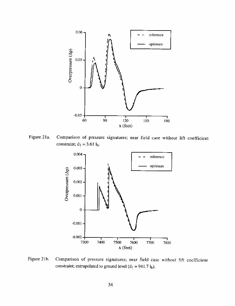
Figure 21 a.
<3
E_©
©
0.06 -
0.03
oJ
-0.03
60
t_ - - reference
!A
I I I I
90 120 150 180
x (feet)
Comparison of pressure signatures; near field case without lift coefficient
constraint; dl = 3.61 lb.
_o
_D;>©
0.004 -
0.003 -
0.002
0.001
-0.001
- - reference
-- optimum
Fk-0.002 i I i i ,
7300 7400 7500 7600 7700 7800
X (feet)
Figure 21 b. Comparison of pressure signatures; near field case without lift coefficient
constraint; extrapolated to ground level (dl -- 941.7 lb).
54

One of the advantages of the design optimization procedure is its applicability to conduct
design trade-off studies. This is illustrated by the results shown above. The two design objectives
of minimum sonic boom and improved aerodynamic performance often impose conflicting
restrictions/variations on the geometric parameters of the aircraft. This is observed to be true while
comparing the two cases described above. In the first case where a constraint on the lift coefficient
is imposed, the optimum design has an improved lift coefficient. The sonic boom signature
associated with this design is also reduced. However, an increase in the second peak is observed.
In the second case where no constraint is imposed on the lift coefficient, the reduction in the first
peak is very significant (compared to the optimum from the previous case) and the second peak is
also reduced. However, the lift coefficient also has decreased. The optimum design shows
significant improvements in CD and CD/CL values compared to the optimum design from the first
case illustrating the trade-off between low sonic boom and high lift configurations. Both sonic
boom overpressures and induced drag increase with an increase in the lift and decrease with a
decrease in the lift. The optimization procedure, in the second case, exploits this important
physical relationship and yields significantly low boom configurations with reduced CL.
Far Field Sonic Boom Minimization ( dl = 941.7 lb )
The results from the optimization of the pressure signature at a distance of 941.7 lb are
presented next. As before, optimization has been performed for minimum sonic boom first peak
(Apl) and minimum CD/CL without any constraint on the lift coefficient. Table 9 compares the
reference and the optimum values of the design variables and the performance functions used in the
optimization. The significant changes to the design variables can be seen. The wing thickness-to-
chord ratio, wing span and nose radius have reduced whereas the wing root chord and nose length
have increased. Figure 22 compares the reference and optimum geometries. Figure 23 compares
the reference and the optimum values of the normalized objective functions. The first peak in the
pressure signature has decreased by 10.2 percent for the optimum configuration. The drag-to-lift
ratio has decreased by 6.0 percent and the drag coefficient has decreased by 9.7 percent. The lift
coefficient has also decreased (3.9 %). The drag force has decreased by 13.1 percent and the lift
force has reduced by 7.2 percent. Figure 24 presents the pressure signatures for the reference and
optimum configurations. The percentage reductions in the optimum far field pressure peaks are not
as significant as those in the near field optima because the far field signature is less sensitive to
changes in the design variables. This is due to the fact that the sonic boom extrapolation procedure
coalesces all the detailed shock information into an N-wave in the far field. This also results in a
higher reduction in the aircraft lift.
55
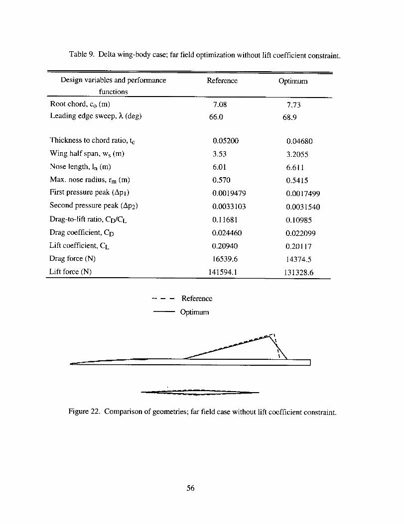
Table9. Deltawing-bodycase;farfield optimizationwithoutlift coefficientconstraint.
Designvariablesandperformancefunctions
Reference Optimum
Rootchord,Co(m)
Leadingedgesweep,_.(deg)
Thicknessto chordratio, tc
Wing half span,Ws(m)
Noselength,In(m)
Max. noseradius,rm(m)
First pressurepeak(Apl)
Secondpressurepeak(Ap2)
Drag-to-liftratio,CD/CL
Dragcoefficient,CD
Lift coefficient,CL
Dragforce(N)
Lift force(N)
7.08 7.73
66.0 68.9
0.05200
3.53
6.01
0.570
0.0019479
0.0033103
0.11681
0.024460
0.20940
16539.6
141594.1
0.04680
3.2055
6.611
0.5415
0.0017499
0.0031540
0.10985
0.022099
0.20117
14374.5
131328.6
Re_nce
Optimum
Figure22.
• i
Comparison of geometries; far field case without lift coefficient constraint.
56

CD/C L
/
AP 1
7
] reference
[] optimum
Figure 23. Comparison of objective functions; far field case without lift coefficient constraint.
O
0.004--
0.003 -
0.002--
0.001 -
0
-0.001 -
-0.002
,\
Reference
Optimum
I I I I I I
2200 2220 2240 2260 2280 2300 2320
x (feet)
Figure 24. Comparison of pressure signatures; far field case without lift coefficient constraint.
57

5.3.6 Doubly Swept Wing-Body Optimization
For the doubly swept wing-body configuration case, the two leading edge sweeps (_,1 and
_,2), the break length (Xb), the wing root chord (Co), the wing tip chord (ct), the maximum nose
radius (rm), the nose length (In) and the wing starting location (Xw) are used as design variables.
The reference values of the doubly swept wing-body parameters are: root chord (Co) = 8.12 m, tip
chord (ct) = 1.62 m, first leading edge sweep (_q) = 70.2 degrees, second leading edge sweep
(_,2) = 54.9 degrees, maximum radius (rm) = 0.57 m, nose length (In) = 6.01 m, break length (Xb)
= 12.28 m, wing starting location (Xw) = 8.13 m, wing span (Ws) = 3.53 m, wing thickness-to-
chord ratio (tc) = 0.05 and body length (lb) = 17.52 m. The wing half span (Ws), the wing
thickness to chord ratio (tc) and the body length (lb) are held constant during the optimization. The
optimization of the doubly swept wing-body configuration has been carried out in two steps. In
the first step, the body radius and nose length are used as design variables to minimize the first
peak in the sonic boom pressure signature. In the second step, the wing geometric parameters are
used as design variables to minimize the second peak in the sonic boom pressure signature, while
the nose dimensions are maintained at their optimum values obtained from the first step. In both
steps, optimization is performed for minimum CD/CL and minimum sonic boom (Apl and Ape) at
a near field distance of dl = 3.61 1b. The lift coefficient is constrained using CLmin = 0.95 CLref
and CLmax = 1.05 CLref where CLref is the lift coefficient of the reference configuration. Table 10
presents the reference and the optimum values of the design variables and the performance
functions used in the optimization.
Figure 25 compares the reference and the optimum geometries. Figure 26 compares the
reference and the optimum values of the normalized objective functions. The first peak in the sonic
boom signature (Apl) has decreased by 23.6 percent in the optimum configuration. This is due to
decrease in the maximum radius (rm) and the increase in the nose length (In) during optimization.
This slender nose has a smaller equivalent area distribution for the nose region yielding a reduced
first pressure peak. Significant increases are observed in the first leading edge sweep, the root
chord and the break length of the optimum wing. These increases coupled with the decreases in
the wing tip chord and starting location result in a smaller planform area for the optimum wing.
The smaller planform area has a smaller equivalent area and lift distribution yielding a significant
reduction (19.9 %) in the second pressure peak of the sonic boom signature. Also, the increase in
the first leading edge sweep of the wing corresponds to a weaker leading edge shock in the wing.
This factor also contributes to the decrease in the second peak (Ap2) of the sonic boom signature.
The CD/CL ratio has also decreased by 3.6 percent in the optimum configuration. This percentage
reduction is small because there are simultaneous reductions in both drag and lift in this case. The
58

drag coefficient hasdecreasedby 4.7 percentandthe dragforce hasdecreasedby 9.2 percent.Thereis alsoadecreasein thelift coefficient(1.1%) andthelift force(4.9%) of theaircraft. The
increasein thefirst leadingedgesweepof the aircraftcorrespondsto a decreasedvalue of theeffectiveMachnumber.Also, theoptimumconfigurationhasa smallerplanformarea.Therefore,
thelift coefficientandthelift havedecreasedfor theoptimumconfiguration.Figures27aand27b
presentthe sonicboompressuresignaturesfor thereferenceandthe optimumconfigurationsat
nearandfar fields, respectively.Thereductionsin thetwopressurepeakscanbeseen.
Table 10. Doublysweptwing-bodycase;nearfield optimizationwith lift constraint.
Designvariablesandperformancefunctions Reference Optimum
Maximumnoseradius,rm(m)
Noselength,In(m)
First leadingedgesweep,_,1(degrees)
Rootchord,Co(m)
Secondleadingedgesweep,_2(degrees)
Tip chord,ct (m)
Breaklength,Xb(m)
Wingstartinglocation,Xw(m)
First pressurepeak
Secondpressurepeak
Drag-to-liftratio,Co/CL
Dragcoefficient
Lift coefficient
Dragforce(N)
Lift force(N)
0.57 0.513
6.01 6.61
70.16 74.25
8.12 8.60
54.93 52.51
1.62 1.39
12.28 12.76
8.13 7.75
0.03389 0.02590
0.05483 0.04394
0.11510 0.11099
0.02238 0.02133
0.19441 0.19221
18558.2 16852.5
159666.9 151843.3
59

...... Reference
Figure 25. Comparison of planforms; near field case with lift coefficient constraint.
0.9
0.8
0.7
0.6
-3.6 %
CD/C L AP t AP2
[] reference
I_1 optimum
Figure 26. Comparison of objective functions; near field case with lift coefficient constraint.
60

C)
0.06
0.03
-0.03I I / I I I
0 10 20 30 40 50 60
X (m)
Reference
Optimum
Figure 27a.
C)
Comparison of pressure signatures; near field optimization with lift coefficient
constraint; dl = 3.61 lb.
0.(KB
0.002
0.001
-0.001 -
- - Reference
Optimum
-0.002 I I J7210 7260 7310 7360
x (feet)
Figure 27b. Comparison of pressure signatures; near field case with lift coefficient constraint;
extrapolated to ground level (dl - 941.7 lb).
61
The optimum designs from the aerodynamic/sonic boom optimization procedure for the two
configurations show a common trend. All these optimum designs are such that the nose region of
these configurations are more slender than their reference nose configurations. Correspondingly,
the first peaks in the pressure signatures of these optimum designs have decreased. This is
contrary to the trends observed by previous optimization studies [80-87] that the nose region
actually becomes more blunt for the sonic boom to decrease. The reasoning given in these studies
behind this trend is that, a blunt nosed configuration with special shaping gives rise to a strong
shock wave which avoids coalition with shocks from other aircraft components, thereby resulting
in a weak wave in the far field. However, the current MDO procedure that couples sonic boom
and aerodynamic criteria, does not compromise aerodynamic performance for sonic boom
improvement and yields slender bodies which have improved sonic boom as well as aerodynamic
characteristics.
5.4 Integrated Aerodynamic/Sonic Boom/Structural Optimization
The fourth MDO procedure developed in this research addresses the simultaneous
improvement in the aerodynamic, sonic boom and structural performance of high speed aircraft
configurations. The procedure uses two-levels of decomposition that are coupled with each other.
Since the sonic boom characteristics of an aircraft are strongly tied in with its aerodynamics, the
performance of the aircraft in these two disciplines is addressed in level 1 of the optimization
procedure. At level 2, the structural performance of the aircraft is optimized. The MDO problem is
formulated as follows.
5.4.1 Optimization Formulation
Level 1
The objectives at this level are reduced sonic boom pressure peaks and improved
aerodynamic performance. This can be stated as follows.
Minimize
Apl, Ap2 and CD/CL
subject to the constraints
CLmin < CL < CLmax
W < Wmax
62
cI:_imin < _I:_l < cI)l max
cI:_2rnin < _2 < cI)2max
where Apl and Ap2 are the overpressure peaks in the sonic boom signature at a distance dl from
the aircraft. The quantity W is the aircraft weight. ¢I)1 is the first level design variable vector, CI:_2
is the second level design variable vector and the subscripts "min" and "max" denote lower and
upper bounds respectively. To incorporate the structural coupling in the first level, constraints are
imposed on the second level objective function, namely the aircraft weight (W) and the second
OW* . _)_)j2anu--, are the optimal sensitivity parameters
level design variables (CI_2). The derivatives, c)(_il O(_il
of the second level objective function and design variables with respect to the first level design
variables. These derivatives establish the coupling between the two-levels of optimization.
Level 2
In the second level, structural optimization of the wing-body configuration is performed
during which, the first level design variables (_1) are held fixed at their optimum values obtained
from level 1 optimization. The optimization problem is defined as follows.
Minimize
W
subject to the following constraints
g(_) < 0
Mx r < Mxrmax
My r < Myrma x
cI_2min < cI_2 < ¢IZD2max
where _ is the stress vector, g(_) is a stress-based failure criterion to determine material failure,
Mx r and My r are the root bending moments along the x and the y directions [Fig. 28], respectively
and subscripts 'min' and 'max' denote lower and upper bounds, respectively. The upper bounds
on the root bending moments are imposed to reduce the loading that is eventually transmitted to the
aircraft. The wing structural parameters are used as design variables during the optimization. The
63

multilevel optimization procedure iterates through the two-levels until global convergence is
achieved.
y
JZ
X
My
T
Figure 28. Nodal force vectors due to aerodynamic loading at a given wing section.
5.4.2 Wing-Body Configuration
The two-level optimization is applied to the design optimization of the doubly swept wing-
body configuration (Fig. 15), described in Section 5.4.4. The reference values of the doube
sweep wing-body parameters are:c o = 8.12 m, c t = 1.62 m, _,l = 70.2 degrees, _ = 54.9 degrees,
rm = 0.57 m, In = 6.01 m, Xb = 12.28 m, Xw = 8.13 m, w s = 3.53 m, tc = 0.05 and lb = 17.52 m.
The wing half span (Ws), the wing thickness to chord ratio (tc) and the body length (lb) are held
constant during the optimization. The two leading edge sweeps (3,1 and _,2), the break length (Xb),
the wing root chord (Co), the wing tip chord (ct), the maximum nose radius (rm), the nose length
(In) and the wing starting location (Xw) are used as design variables during optimization at level 1.
5.4.3 Structural Model and Analysis
The principal load carrying member in the wing is modeled as a single-celled composite
box beam, as illustrated in Fig. 29. The structural design variable vector (_2) includes the box
beam width to chord ratio (Wc) and the ply angles (0%) of the laminates used to form the box beam
walls (Fig. 29). The box beam width to chord ratio (Wc) is a continuous design variable whereas
the ply angles are discrete variables, taking on discrete values from the set (0 °, +15 °, +30 °, +45 °,
+60 ° , +75 ° and +90°).
The analysis procedure for such composite beams is based on the formulation developed by
Smith and Chopra [125]. The analysis procedure allows the inclusion of pre-twist, taper and
spanwise sweep in the box beam. Using the analytical model, the deformation of the beam is
64

describedthroughextension,bending,torsion,transverseshearingandtorsionrelatedwarping. In
the presentwork, this quasionedimensionalmodel is usedwithin a finite elementanalysistoobtainnodaldeflectionsandstressesin theloadcarryingmember.Thebeamhasbeendividedinto
10elementsover thewing span.Thei thfinite elementisboundedby thenodesi (z = zi) andi+l
(z = zi+l). Eachfinite elementhas19degreesof freedom,Ue, which aredescribedasfollows
[Fig. 30].
UeT= [ Ul,U2,U3,U4,Vbl,Vb!,Vb2,Vb2,Wb1,wbI , Wb2,Wb2,_)1,_)2,(_3,
vsl,Vs2,Wsl,Ws2] (54)
width
cg=centroid(xcg,ycg,zcg)
/////////
ffJfJfJJJ
,N\\\\\\\
012
01
0t
012
Figure 29. Composite box beam model.
In Eq. 54, u is the spanwise wing displacement, v and w are the inplane vertical and horizontal
wing displacements and _ is the elastic twist. First partial derivatives with respect to the spanwise
coordinate (z) are denoted ('). The inplane wing displacements are expressed as a sum of two
terms, one corresponding to pure bending and another corresponding to shear. In Eq. 54, the
subscript (b) refers to the displacements due to beam bending and the subscript (s) refers to the
displacements due to shear.
65
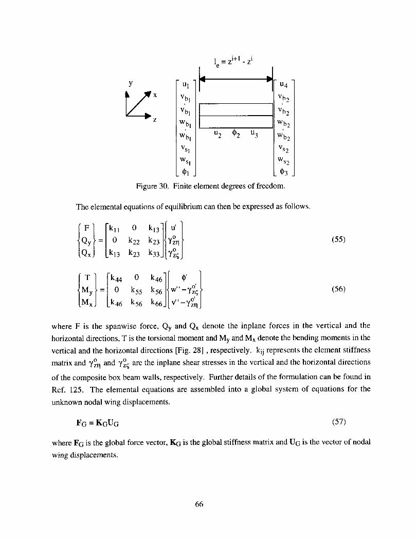
1 = z i+l - z ie
Ly ul r
vb,I,Vb 1
z Wb 1T
Wb 1
Vs I
Ws 1
ool
Figure 30.
u2 002 u3
w
u4
i Vb2
' V'b2
[Wb 2
Wb 2
Vs 2
Ws 2
003
Finite element degrees of freedom.
The elemental equations of equilibrium can then be expressed as follows.
Qy = k22 _=3/_t
Qx Lkl3 k23 k333[T°_J
{T}MyFko40k461r0',1= k55 k5611w"-_'!_
Mx Lk46 k56 k66j[v"-y°zrlJ
(55)
(56)
where F is the spanwise force, Qy and Qx denote the inplane forces in the vertical and the
horizontal directions, T is the torsional moment and My and Mx denote the bending moments in the
vertical and the horizontal directions [Fig. 28], respectively, kij represents the element stiffnesso o
matrix and 7zq and Yz_ are the inplane shear stresses in the vertical and the horizontal directions
of the composite box beam walls, respectively. Further details of the formulation can be found in
Ref. 125. The elemental equations are assembled into a global system of equations for the
unknown nodal wing displacements.
FG = KGUG (57)
where FG is the global force vector, KG is the global stiffness matrix and UG is the vector of nodal
wing displacements.
66

5.4.4 Aerodynamic Load Calculations
The finite element method for the aircraft wing structural analysis requires the nodal load
vectors to be specified. Clearly, the loading on the wing structure comes from the aerodynamic
forces and moments that act on the surface of the wing. The pressure distribution on the wing,
which gives rise to these forces and moments, is obtained from the UPS3D flow solver. These
forces and moments are expressed as follows.
Q_= j_-p(x,y,z)ds x (58)i+l
Si
Q_: _-p(x,y,z)dsy (59)i+l
Si
F' = _-p(x,y,z)ds z (60)i+l
Si
M_¢= jJ-p(x,y,z)(z-Zicg)dsyi+l
S i
(61)
M_¢= jj-p(x,y,z)(z-Z_g)dsxi+l
Si
(62)
Tl= j'J -p(x, y,z)[(x-X_g)dsy +(y-y_g)ds x ]i+l
Si
(63)
In Eqs. 58-63, p(x,y,z) is the local pressure, dsx, dsy and dsz are the projections of an elemental
wing surface area element (dS) in the x, y and z directions, respectively and __!+1 denotes the areai i
segment between the finite element nodes i (z = z i) and i+l (z = zi+l). The quantities Xcg, Ycg
iand Zcg are the x, y and z coordinates of the centroid of the beam section at node i (z = z i) (Fig.
29). Since a symmetric composite box beam is used at every station throughout the span, the
centroid corresponds to the center of the box beam section (Fig. 29).
The Tsai-Wu failure criterion [ 126] has been used in the second level optimization to avoid
composite material failure. This criterion is expressed as follows.
67
( II 11 1_ +1 1 O2T O2C ) O1TO1cOi T O! C O1 + O 2
0 2 O10 2 'i722+ +--<0
O2TO2 C _O1TO1CO2TO2 C '_122S
(64)
where a I and O 2 represent normal stresses along the material axes and 'I;12 represents the shear
stress. The subscripts T, C and S represent ultimate stress in tension, compression and shear,
respectively. The Tsai-Wu criterion reduces the total number of constraints as individual
constraints on the stresses (o 1, o 2 and _12) at each ply are eliminated. Each of the four composite
plates used in the box beam modeling is assumed to be symmetric about the midplane of the plate
and the beam itself is assumed to be symmetric about the beam centerline. The above failure
criterion is imposed, on each lamina, at each of the four comers of the box beam to prevent failure
due to stresses.
5.4.5 Weight Calculations
The aircraft weight (W) is calculated as the sum of the fuselage skin weight (Wfus), the
wing skin weight (Wwsk) and the wing spar weight (Wwsp). The skin is assumed to be made of
2014-T6 Aluminum alloy. The composite box beam is assumed to be made of Carbon-Epoxy
IM6/Epoxy. This material has a density of 1600 Kg/m 3 and its ultimate stresses are given by O1T
= 3500 MPa, O1C = 1540 MPa, O2T = 56 MPa, O2C = 150 MPa, '1712S = 98 MPa. The box beam
vertical wall thickness (tv) is 0.0366 m and the horizontal wall thickness (tw) is 0.0366 m. These
two parameters are held fixed during the optimization. The expressions for Wfus, Wwsk, Wwsp are
as follows.
W = Wfus + Wwsk + Wwsp
Wfus = rm(lb-ln)+ r(x)dx _tskPskg
Wws k = Ic(z)dz tskPskg
rm
(65)
(66)
(67)
W s
Wwsp = 9spg * [ - 4thtv(Ws-rm)+ 2[Wcth+tc(1- Wc)tv] _c(z)dz ]
r m
(68)
68

wheretskis theskinthickness,Pskis thedensityof theskinmaterial,9spis thedensityof thewing
sparmaterial,c(z)is thelocalchordat anyspanwisewingsectionz andg is theaccelerationdueto
gravity.
5.4.6 Optimization Algorithms
In level 1, all the design variables are continuous and a nonlinear quasi Newton technique
which uses the BFGS algorithm [108] for finding the search direction is used. The structural
optimization problem at the second level involves a design variable vector that includes both
continuos design variables _c (e.g., spar width-to-chord ratio) and discrete design variables _cl
(e.g., ply angles). Continuos design variables are not compatible with combinatorial optimization
methods such as branch and bound techniques which require discrete values to operate. Similarly,
discrete variables are not compatible with gradient-based optimization methods unless a continuous
relaxation of the discrete variables is allowed which may lead to sub-optimal solutions. Thus,
optimization problems with both continuous and discrete design variables require the development
of a technique which efficiently incorporates both types of design variables. Chattopadhyay and
Seeley [127] have recently developed a hybrid optimization technique which can efficiently include
both continuous and discrete design variables. This procedure uses both a gradient-based search
and a modified simulated annealing algorithm to obtain a more global optimum. The technique is
briefly outlined below.
1. START
2. Current value of objective function is F
3. Select either continuous or discrete design variables to perturb for Fnew
4. If continuous variables are selected,
(I)cnew - (I) c + _S c
5. If discrete variable is selected
(I)dnew = (I)di
6. Compute Fnew
7. If Fnew < F then
F = Fnew
Else if Pacc> P then
F = Fnew
Endif
8. Check for convergence
9. If no convergence, go to START else STOP
69

Here,thequantityF is thecurrentvalueof theK-S function, c_is arandomstepsizeselectedto be
within aprescribedpercentageof thecurrentvalueof thecontinuousvariablesandS is thesearchdirectionvectorwhich is determinedfrom thegradientsof the K-S function with respectto the
continuousdesignvariables.Thesubscripti refersto the i th choice for a discrete design variable
out of a set of discrete values and the subscript 'new' stands for a new design point. The
continuous design variables are perturbed using o_ and S to improve the efficiency of the search
while the discrete variables are perturbed by randomly selecting values for CI_di within a given set.
Move limits and bounds are imposed on the continuous design variables to ensure a physically
meaningful design. The parameter P is a random number such that 0 < P < 1 and the acceptance
probability (Pacc) of retaining a worse design is computed as follows.
Pacc = exp(-AF/T) (69)
where AF represents the change in objective function and T is the "temperature" which is computed
at each iteration using the following relation.
T = Toq i (70)
where the temperature T is reduced from the initial temperature To during successive iterations i
using the cooling rate q (0 < q < 1). A high temperature allows the optimizer to occasionally accept
a design for which the objective function (Fnew) value is worse than the reference value. The
worse design is accepted based on the acceptance probability probability and allows the algorithm
to climb out of local minima. The acceptance probability is gradually reduced to zero during
optimization so that the optimizer converges smoothly to an improved design point.
The hybrid optimization procedure relies on a directed search for the continuous design
variables which increases efficiency. However, the probabilistic nature of the simulated annealing
algorithm allows the optimization procedure to climb out of local minima. Therefore, the
procedure exhibits the benefits of both gradient-based and discrete optimization techniques.
5.4.7 Results and Discussion
The optimization at level 1 has been carried out in two steps. In the first step, the body
radius and nose length are used as design variables to minimize the first peak in the sonic boom
pressure signature. In the second step, the wing geometric parameters are used as design variables
to minimize the second peak in the sonic boom pressure signature, while the nose dimensions are
maintained at their optimum values obtained from the first step. In both steps, optimization is
performed for minimum CD/CL and minimum sonic boom (Api and Ap2). The lift coefficient is
70

constrainedusingCLmin = 0.95 CLre f and CLmax = 1.05 CLref where CLref is the lift coefficient of
the reference configuration. The inviscid flow field around the vehicle is evaluated using the CFD
solver (UPS3D) over a streamwise distance that extends from the tip of the body up to three times
the body length in the longitudinal direction. The aerodynamic sensitivity analysis at level 1 is
performed using the semi-analytical sensitivity analysis techniques [94-95]. The sensitivity
analysis at level 2 is performed using the finite difference method. A three-dimensional hyperbolic
grid with 75 grid points in the circumferential direction and 80 grid points in the normal direction
has been used. The cruise Mach number is 2.5, the angle of attack is 5 degrees and the flight
altitude is approximately 16,500 m. The aircraft weight (W) is constrained during the level 1
optimization to be below Wmax = Wref where Wref is the weight of the reference configuration.
The pressures at do = 0.5 lb are directly obtained from the CFD solver. The sonic boom signatures
at two locations have been considered during the optimization. The first of the two corresponds to
a distance dl= 3.61 lb from the axis of the body and is denoted "near field" in the text. The
second distance considered is dl = 941.7 lb from the axis of the body and is denoted "far field."
This far field distance corresponds to the ground level. Results from both cases of optimization are
discussed here.
Near Field Optimization (d! = 3.61 lb)
Figure 31 compares the reference and the optimum geometries. Figure 32 compares the
reference and the optimum values of the level 1 objective functions normalized with respect to their
corresponding reference values.
m
m
Reference
Near field optimum ," "
m
Figure 31.
I..
Comparison of planforms; near field optimization.
The first peak in the sonic boom signature (Apl) decreases by 23.6 percent in the optimum
configuration. This is due to the decrease in the maximum radius (rm) and the increase in the nose
length (In) during optimization. This slender nose has a smaller equivalent area distribution for the
nose region yielding a reduced first pressure peak. The smaller planform area of the optimum
configuration has a smaller equivalent area and lift distribution. The increase in leading edge
sweep (L1) of the optimum configuration also results in a weaker wing shock. These factors yield
a significant reduction (18.7 %) in the second pressure peak (Ap2) of the sonic boom signature.
71

TheCD/CL ratio has also decreased by a modest 3.5 percent in the optimum configuration. This
percentage reduction is small because there are simultaneous reductions in both drag and lift in this
case. Figure 33 presents the sonic boom pressure signatures for the reference and the optimum
configurations. The constraint imposed on the aircraft weight (W) during the level 1 optimization
is satisfied throughout the optimization.
Table 11 presents the reference and the optimum values of the design variables and the
performance functions used in the level 1 optimization. Significant increases are observed in the
first leading edge sweep, the root chord and the break length of the optimum wing. These
increases coupled with the decreases in the wing tip chord and starting location result in a smaller
planform area for the optimum wing.
Table 11. Comparison of level 1 design variables and objective functions.
Design Variables Reference Near field Far field
optimum optimum
Maximum nose radius, rm (m)
Nose length, In (m)
1st leading edge sweep, XI (deg)
Root chord, Co (m)
2 nd leading edge sweep, X2 (deg)
Tip chord, ct (m)
Break length, Xb (m)
Wing starting location, Xw (m)
First pressure peak (Ap!)
Second pressure peak (Ap2)
Drag-to-lift ratio, CD/CL
0.570 0.513 0.513
6.010 6.610 6.610
70.20 74.40 70.32
8.120 8.610 8.060
54.93 52.45 59.75
1.620 1.355 1.240
12.28 12.44 11.27
8.130 7.670 7.150
0.03389 (Near) 0.02590 0.00120
0.00136 (Far) (-23.6 %) (-11.9 %)
0.05483 (Near) 0.04459 0.00258
0.00269 (Far) (-18.7 %) (-3.9 %)
0.11510 0.11112 0.10983
(-3.5 %) (-4.6 %)
72

1-/
0.95-
0.9-
0.85 -
0.8-
0.75 -
0.7 _"
_ Reference
Near field optimum
Far field optimum
I I
AP1 AP2 CD/CL
Figure 32. Comparison of level 1 objective functions.
o
0.06--
0.045 -
0.03-
0.015 -
0
-0.015
-0.03
Reference
Near field optimum
I I I I I I I I I I
15 20 25 30 35 40 45 50 55 60 65
x (m)
Figure 33. Comparison of pressure signatures; near field optimization.
Structural optimization is performed in level 2. As mentioned earlier, the walls of the
composite box beam have 24 plies which are symmetrically oriented about the midsection of the
wall. The corresponding 12 ply orientations and the beam width-to-chord ratio (wc) have been
used as design variables. Constraints on the stresses in the plies at all the spanwise finite element
73

nodes are imposed through the Tsai-Wu criterion. The reference values are used as the upper
bounds for the wing root bending moment constraints, that is, Mxrmax = Mxrref and Myrma x =
Myrre f. The level 2 optimization is initiated with all the 12 ply angles set to the reference value of
90 degrees. Table 12 compares the reference and the optimum values of the design variables and
the aircraft weight obtained from the level 2 optimization. Considerable reduction (10 percent) in
the aircraft weight is observed from the reference to the optimum configuration.
Figure 34 compares the reference and the optimum values of the aircraft weight normalized
with respect to the reference weight and shows the corresponding reductions in the fuselage, wing
skin and wing spar weights. The aircraft weight reduction is due in part to the reductions in the
fuselage weight (11.2 percent) and the wing skin weight (2.1 percent), associated with the changes
in the level 1 design variables during the level 1 optimization. The reduction in the wing skin
weight is relatively small because the reduction in the wing planform area is relatively small.
Weight reduction is also obtained through a reduction in the wing spar weight (18.2 percent). The
optimum spar width-to-chord ratio (Wc) has reduced by 16.1 percent to effect this change. In the
reference configuration, the stress constraints are violated within several plies at various spanwise
locations. The optimization procedure is able to modify these stresses through significant changes
to the ply stacking sequence. The modified stress distribution in the optimum box beam
configuration satisfies the Tsai-Wu criteria at all the plies at all spanwise finite element nodes. The
optimum configuration also satisfies the root bending moment constraints well. Figure 35
compares the stresses and the root bending moments in the plies of the reference and the optimum
beam configurations for the root section. It is to be noted the stresses and the bending moments
have been normalized using their corresponding reference values. Significant reductions are
observed in both the root stresses and the root bending moments after the optimization.
74

Table 12. Comparison of level 2 design variables and objective function(s).
I
Reference weight ] 1999.6 N
Near field optimum I 1799.8 N (-10 %)Far field optimum 1737.5 N (-13 %)
Design Wc 01 02 03 04 05 06 07 08 09 010 011 012
variable.
Reference 0.50 90 ° 90 ° 90 ° 90 ° 90 ° 90 ° 90 ° 90 ° 90 ° 90 ° 90 ° 90 °
Near field 0.42 75 ° 75 ° -75 ° 90 ° 75 ° 90 ° 90 ° 90 ° -75 ° -75 ° 75 °
60 °
Far field 0.43 75 ° 75 ° -75 ° 90 ° 90 ° 90 ° 90 ° 90 ° 90 ° -75 ° 75 °
75 °
1 m
0.95 -
0.9-
0.85-
0.8
0.75
0.7
_ Reference
Near field optimum
Far field optimum
2.1%
11.2%
m
I I I
W Wfm Wws k Wws p
Figure 34. Comparison of level 2 objective function(s).
75
Far Field Optimization (dl = 941.7 Ib)
The far field optimization formulation is identical to that the near field optimization except
that the sonic boom pressure peaks (Apl and Ap2) are evaluated at dl = 941.7 lb. Table 11
presents the reference and the optimum values of the design variables and the performance
functions used in the level 1 optimization. Figure 36 compares the reference and the optimum
geometries. Figure 32 compares the reference and the optimum values of the level 1 objective
functions normalized with respect to their corresponding reference values. The first peak in the
sonic boom signature (Apl) has decreased by 11.9 percent in the optimum configuration. Similar
to the near field optimization case, this is due to the decrease in the maximum radius (rm) and the
increase in the nose length (In) during optimization. In fact, it can be noticed that both the near
field and the far field optimizations yield the same optimum values for these two design variables.
However, the changes in the wing planform variables show different trends in the far field
optimization. Unlike the near field case, there is relatively small changes in the first leading edge
sweep (_,l) and the wing root chord (Co). The tip chord (ct) has decreased significantly (23.4
percent) and the second leading edge sweep (_2) has increased (8.1 percent). The wing starting
location (Xw) has moved forward by a significant 12.1 percent and the break length (Xb) has
decreased by 8.2 percent. These factors yield only a modest reduction (3.9 %) in the second
pressure peak (Ap2) of the sonic boom signature. These design trends indicate that the far field
sonic boom signature is relatively less sensitive to design variable changes than the near field
signature. This is due to the fact that the sonic boom extrapolation procedure [ 124] tries to fit an
approximate N-wave to the sonic boom signature at far field distances. The extrapolation
procedure coalesces all the detailed shock information into the N-wave in the far field and makes it
less sensitive to changes in the design variables. The CD/CL ratio has decreased by 4.6 percent in
the optimum configuration.
76

_ Reference
Near field optimum
Far field optimum
1 m
0.93--
0.86--
0.79-
0.72
/--- /---- /----
u2.
m
/----
_t _t
o I 0 2 x12 M x My
35. Comparison of normalized root stresses and bending moments.
Figure
Figure 37 presents the sonic boom pressure signatures for the reference and the optimum
configurations. Since the wing starting location and the break length have decreased for the
optimum configuration [Fig. 36], the relative separation between the first and the second sonic
boom overpressure peaks has also decreased for the optimum configuration. This can be clearly
seen in Fig.37 for the optimum pressure signature.
m
Reference
Far field optimum
I
_ _ _ .]L __
Figure 36. Comparison of planforms; far field optimization.
77

0.003 -
0.002 -
0.001r_
E_;- 00
-0.00!
m m
Referencem
Far field optimum
-0.002 I = I I I I7200 7230 7260 7290 7320 7350 7380
x (m)
Figure 37. Comparison of pressure signatures; far field optimization.
The reference design for the level 2 (structural) optimization has the 12 ply angles set equal
to 90 degrees. Table 12 compares the reference and the optimum values of the design variables
and the aircraft weight obtained from the level 2 optimization. The optimization procedure reduces
the weight significantly (13 percent). Figure 34 compares the reference and the optimum values of
the aircraft weight normalized with respect to the reference weight and shows the significant
reduction in the total weight and its components. The fuselage weight, the wing skin weight and
the wing spar weight have decreased by 11.2 percent, 22.1 percent and 13.9 percent, respectively.
Unlike the near field case, the wing skin weight has reduced significantly in this case because the
planform area of the far field optimum configuration is considerably smaller than the planform area
of the reference configuration. The stress distribution in the optimum configuration satisfies the
Tsai-Wu criteria at all the plies and at all spanwise finite element nodes. The optimum
configuration also satisfies the root bending moment constraints. Figure 35 compares the stresses
and the root bending moments in the plies of the reference and the optimum beam configurations
for the root section. The optimization procedure successfully reduces the stresses and the root
bending moments in all the plies. However, the reduction in the root bending moments are mainly
due to the reductions in the aerodynamic loading corresponding to the decreases in the drag and the
lift forces of the wing-body. The values of the root bending moments are dictated by the
aerodynamic loading. If an "all-at-once" approach is used to perform the multidisciplinary
optimization instead of the present multilevel decomposition technique, these root bending moment
constraints would play an important role during optimization.
78
FromTable 12,it canbeobservedthat in level2, thenearfield optimumandthe far field
optimumleadto similardesignvariablechanges.Oneof themainreasonsfor this trendis thatthe
aerodynamicloaddistributions,obtainedafterlevel 1optimization,aresimilarto eachotherin boththenearfield andthefar field cases.Therefore,thechangesin the level2 designvariablesshow
similar trendsin bothcases.
6. Concluding Remarks
A semi-analytical sensitivity analysisprocedurehasbeen developedfor calculating
aerodynamic design sensitivities to be used in design optimization problems involving
comprehensiveCFDsolvers.Thegrid sensitivitiesandtheflow variablesensitivitiesarecalculated
by directlydifferentiatingthediscretizedgovemingdifferentialequations.Theprocedurehasbeendevelopedfor thethree-dimensionalPNSsolver,UPS3D.Theaerodynamicdesignsensitivitiesof
wing-bodyconfigurationshavebeencalculatedusingthedevelopedprocedure.Thecomputational
grid usingwithin UPS3Dincludes75pointsin thecircurrnferentialdirectionand80pointsin thenormaldirection. Resultsobtainedfrom thesemi-analyticalsensitivitytechniquescompareverywell with thoseobtainedusingafinite differenceapproach.Whenthesemi-analyticalsensitivity
analysistechniquesareusedinsteadof a finite differenceapproachwithin designoptimization
procedures,theseCPUsavingsbecomeverysignificant. For atypical sensitivityanalysisusing
four designvariables,the procedureyields a 39percentreductionin CPU time over the finitedifferencetechnique.Within theintegratedaerodynamic/structuraloptimizationof thedeltawing-
body configurationwherethesefour designvariablesareused,the semi-analyticalsensitivityanalysistechniquesdecreasethe CPUtime by 780secondsperdesigncycleon theCRAY 2 or
nearly6.5CPUhoursfor theentireoptimization.Duringtheintegratedaerodynamic/sonicboom
optimizationof thedeltawing-bodyconfigurationwheresix designvariablesareused,thesemi-
analyticalsensitivityanalysistechniquesoffer asavingsof 2595secondsperdesigncycle (35 %)and approximately 7 CPU hours for the entire optimization. During the integrated
aerodynamic/sonic boom optimization of the doubly swept wing-body configuration where eight
eight design variables are used, the semi-analytical sensitivity analysis techniques offer a savings
of 3460 seconds per design cycle (36.2 %). The time required for the entire optimization decreases
by I l CPU hours due to these CPU savings. Thus, there are two important observations to be
made of the semi-analytical sensitivity analysis technques.
.
.
Significant savings in CPU time are realized by using these techniques instead of the finite
difference approach, without any loss in accuracy.
The reduction in CPU time for each sensitivity analysis increases as the number of design
variables increases.
79

Thesecondobservationis of importantconsequencein apracticaldesignenvironment,wherea
large of designparametersmay be usedto definethe aircraft. In sucha situation, the semi-
analytical sensitivity analysisprocedurewill be able to savea very significant amount of
computationaltime. Thesavingsassociatedwith thesemi-analyticalapproachalsoallows theuseof comprehensiveanalysisprocedures(three-dimensionalNavier Stokessolvers)within design
optimization.Several multidisciplinary design optimization procedureshave been developed for
aerospaceapplications. The MDO proceduresfor high speedconfigurationssimultaneously
improve the aerodynamic,sonic boom and structuralperformanceof the aircraft. The three-dimensional,supersonicflow aroundtheaircraft iscalculatedusingthePNSsolver,UPS3D. The
wing loadcarryingmemberis modeledaseitheranisotropicboxbeamor a compositeboxbeam.The isotropicbox beammodel is analyzedusingthin wall theoryandthecompositebox beam
modelis analyzedusingafiniteelementapproach.Theaerodynamicdesignsensitivitieshavebeen
calculatedusingthesemi-analyticalsensitivityanalysistechniques.A two-level decomposition
procedureis usedwhenstructuralcriteriaareincludedwithin theoptimizationformulation. Thefollowing summarizestheresultsfromtheoptimizationprocedures.
.
,
.
.
.
The integrated aerodynamic/structural optimization procedure for high speed wing-body
configurations yields significant reductions in the aircraft drag and weight while improving
the lift.
The reduction in the aircraft drag is predominantly due to the significant reduction in the
wing thickness-to-chord ratio. The improvement in the lift is due to the increased planform
area caused by the increases in the wing root chord and wing span. Reduction in the
aircraft weight is achieved through reductions in the wall thicknesses of the wing spar.
The multiobjective optimization procedures, for integrated aerodynamic/sonic boom
optimization and the two-level optimization procedure, for integrated aerodynamic/sonic
boom/structural optimization, are efficient and yield overall improvements in all the
performance criteria included in the formulations.
Contrary to prior investigations, the multidisciplinary procedures yield low boom
configurations that are more slender and hence, aerodynamically efficient. Reductions in
the first peak of the sonic boom pressure signature are achieved through significant changes
to the nose dimensions of the aircraft. Reduction in the second pressure peak is achieved
through changes to the wing planform geometry and thickness-to-chord ratio.
The procedure demonstrates the trade-offs between low boom and aerodynamically
efficient configurations. The low boom designs have decreased lift associated with them.
80

.
.
The percentage reductions in the sonic boom overpressure peaks are smaller for
optimizations based on the far field signature than those based on the near field signature.
The aircraft weight is affected both by the planform variables as well the beam width-to-
chord ratio. The stresses in the plies and the root bending moments are significantly
reduced during the optimization through a redistribution of the ply stacking sequence.
The MDO procedures, coupled with the sensitivity analysis techniques, have been found to
be efficient and reliable tools for the design of aerospace systems. The procedures are capable of
optimizing complete configurations as well as individual components. They bring out the trade-
offs between the individual disciplines. They also help identify design parameters that are
ineffective during the optimization and hence, can be eliminated from the design variable set. They
can be extremely useful tools to the designer by providing insight into the influence of each design
variable on the overall performance of the system. The semi-analytical sensitivity analysis
techniques offer significant computational savings and allow comprehensive analysis procedures
(e.g., Navier Stokes solvers) to be coupled within design optimization.
References
.
.
.
.
.
.
,
.
Sobieszczanski-Sobieski, J. and Loendorf, D., "A Mixed Optimization Method for
Automated Design of Fuselage Structures," Journal of Aircraft, Vol. 9, No. 12, December,
1972, pp. 805-811.Fulton, R. E., Sobieszczanski, J., Storaasli, O., Landrum, E. J. and Loendorf, D.,
"Application of Computer-Aided Aircraft Design in a Multidisciplinary Environment,"
Proceedings of the 14 th AIAA/ASME/SAE Structures, Structural Dynamics and MaterialsConference, Williamsburgh, Virginia, 1973.Barthelemy, J. F. M., Coen, P. G., Wrenn, G. A., Riley, M. F., Dovi, A. R. and Hall,L. E., "Application of Multidisciplinary Optimization Methods to the Design of aSupersonic Transport," NASA TM-104073.Barthelemy, J. F. M., Wrenn, G. A., Dovi, A. R. and Coen, P. C., "Integrating
Aerodynamics and Structures in the Minimum Weight Design of a Supersonic Transport
Wing," 33 rd AIAA/ASME/AHS/ASCE Structures, Structural Dynamics and Materials
Conference, Dallas, Texas, 1992.Dovi, A. R., Wrenn, G. A., Barthelemy, J. F. M., Coen, P. G. and Hall, L. E.,"Multidisciplinary Design Integration Methodology for a Supersonic Transport Aircraft"Journal of Aircraft, Vol. 32, No. 2, March-April, 1995, pp. 290-297.Celi, R. and Friedmann, P. P., "Structural Optimization with Aeroelastic Constraints ofRotor Blades with Straight and Swept Tips," AIAA Journal, Vol. 28, No. 5, 1990, pp.928-936.Chattopadhyay, A., Walsh, J. L. and Riley, M. F., "Integrated Aerodynamic/DynamicOptimization of Helicopter Blades," Special Issue of the AIAA Journal of Aircraft onMultidisciplinary Optimization of Aeronautical Systems, Vol. II, 1991, pp. 58-64.Chattopadhyay, A. and Narayan, J. R., "Optimum Design of High Speed Prop-Rotors
Using a Multidisciplinary Approach," Presented at the 48 th Annual Forum of the American
Helicopter Society, Washington D. C., June, 1992.
81

.
10.
11.
12.
13.
14.
15.
16.
17.
18.
19.
20.
21.
22.
Chattopadhyay, A. and Narayan, J. R., "A Design Optimization Procedure for High Speed
Prop-Rotors," AIAA Paper No. 92-2375, Proceedings of the 33 rdAIAA/ASME/ASCE/AHS Structures, Structural Dynamics and Materials Conference,
Dallas, Texas, April, 1992.Chattopadhyay, A., McCarthy, T. R. and Madden, J. F., "A Design OptimizationProcedure for Minimizing Drive System Weight of High Speed Prop-Rotors," Presented at
the 4 th AHS Specialists Meeting on Multidisciplinary Optimization, Atlanta, Georgia,
April, 1993.Chattopadhyay, A., McCarthy, T. R. and Madden, J. F., "Structural Optimization of HighSpeed Prop-Rotors Including Aeroelastic Stability Constraints," Mathematical ComputerModelling, Vol. 18, No. 314, 1993, pp. 101-114.Chattopadhyay, A., McCarthy, T. R. and Madden, J. F., "An Optimization Procedure forthe Design of Prop-Rotors in High Speed Cruise Including the Coupling of Performance,Aeroelastic Stability and Structures," Mathematical Computer Modelling, Vol. 19, No. 3/4,
1994, pp. 75-88.McCarthy, T. R. and Chattopadhyay, A., "Multidisciplinary Optimization of HelicopterRotor Blades Include Design Variable Sensitivity," Presented at the 4 th
AIAA/USAF/NASA/OAI Symposium on MuItidisciplinary Analysis and Optimization,
Cleveland, Ohio, September, 1992.McCarthy, T. R. and Chattopadhyay, A., "Design of High Speed Prop Rotors UsingMultiobjective Optimization Techniques," AIAA Paper No. 93-1032, Proceedings of the1993 AIAA/AHS/ASEE Aerospace Design Conference, Irvine, California, February,
1993.Cramer, E. J., Frank, P. D., Shubin, G. R., Dennis, Jr., J. E. and Lewis, R. M., "OnAlternative Problem Formulations for Multidisciplinary Design Optimization," AIAA Paper
No. 92-4752, Presented at the 4 th AIAA/USAF/NASA/OAI Symposium on
Multidisciplinary Analysis and Optimization, Cleveland, Ohio, September, 1992.Sobieszczanski-Sobieski, J. and Balling, R. J., "Optimization of Coupled Systems: A
Critical Overview of Approaches," AIAA Journal, Vol. 34, No. 1, January, 1996, pp. 6-11.
Schmit, L. A. and Merhinfar, M., "Multilevel Optimum Design of Structures with Fiber-
Composite Stiffened-Panel Components," AIAA Journal, Vol. 20, No. 1, 1982, pp. 138-147.
Schmit, L. A. and Chang, K. J., "A Multilevel Method for Structural Synthesis," 25 thAIAA/ASME/AHS/ASCE Structures, Structural Dynamics and Materials Conference, Palm
Springs, California, 1984.
Hughes, O. F., "A Method for Nonlinear Optimum Design of Large Structures andApplications to Naval Ship Design," Proceedings of the International Symposium onOptimum Structural Design, Tucson, Arizona, October, 1981.
Sobieszczanski-Sobieski, J., "A Linear Decomposition Method for Large Optimization
Problems - Blueprint for Development," NASA TM 83248, February, 1982.
Sobieszczanski-Sobieski, J., James, B. and Dovi, A. R., "Structural Optimization by
Multilevel Decomposition," AIAA Journal, Vol. 23, November, 1985, pp. 1775-1782.
Sobieszczanski-Sobieski, J., James, B. and Riley, M. F., "Structural Optimization by
Generalized, Multilevel Optimization," 26 th AIAA/ASME/AHS/ASCE Structures,
Structural Dynamics and Materials Conference, Orlando, Florida, 1985.
82

23.
24.
25.
26.
27.
28.
29.
30.
31.
32.
33.
34.
35.
36.
37.
38.
Sobieszczanski-Sobieski,J., James,B. and Riley, M. F., "Structural Optimization byGeneralized,Multilevel Decomposition,"AIAA Journal, Vol. 25, January, 1987, pp. 139-145.
Wrenn, G. A. and Dovi, A. R., "Multilevel/Multidisciplinary Optimization Scheme for
Sizing a Transport Aircraft Wing," Proceedings of the 28 th AIAA/ASME/ASCE/AHSStructures, Structural Dynamics and Materials Conference, Monterey, California, April,1987.
Haftka, R. T., "An Improved Computational Approach for Multilevel Optimum Design,"Journal of Structural Mechanics, Vol. 12, No. 2., 1984, pp. 245-261.
Kirsch, U., "An Improved Multilevel Structural Synthesis Method," Journal of StructuralMechanics, Vol. 13, No. 2, 1985, pp. 123-144.
Barthelemy, J. F. M. and Riley, M. F., "Improved Multilevel Optimization Approach forthe Design of Complex Engineering Systems," AIAA Journal, Vol. 26, No. 3, 1988, pp.353-360.
Barthelemy, J. F. M., "Engineering Applications of Heuristic Multilevel OptimizationMethods," NASA TM 101504, October, 1988.
Bloebaum, C. L. and Hajela, P., "Heuristic Decomposition for Non-Hierarchical
Systems," 32 nd AIAA/ASME/AHS/ASCE Structures, Structural Dynamics and MaterialsConference, AIAA Paper 91-1039, Baltimore, Maryland, 1991.
Rogan, J. E. and Kolb, M. A., "Application of Decomposition Techniques to thePreliminary Design of a Transport Aircraft," NASA CR 178239, February, 1987.
Adelman, H. M., Walsh, J. L. and Pritchard, J. I., "Recent Advances in Integrated
Multidisciplinary Optimization of Rotorcraft," AIAA Paper 92-4777, 4 th
AIAA/USAF/NASA/OAI Symposium on Multidisciplinary Analysis and Optimization,Cleveland, Ohio, 1992.
Chattopadhyay, A., McCarthy, T. R. and Pagaldipti, N., "Multilevel DecompositionProcedure for Efficient Design Optimization of Helicopter Rotor Blades," AIAA Journal,
Vol. 33, No. 2, February, 1995, pp. 223-230. Also presented as Paper n°G7, 19 th
European Rotorcraft Forum, Italy, 1993.Chattopadhyay, A., McCarthy, T. R. and Seeley, C. E., "A Decomposition BasedOptimization Procedure for High Speed Prop-Rotors Using Composite Tailoring andSimulated Annealing," Journal of Aircraft, Vol. 32, No. 5, 1995, pp. 1026-1033.Sobieszczanski-Sobieski, J., Barthelemy, J. F. M. and Riley, M. F., "Sensitivity of
Optimum Solutions to Problem Parameters," AIAA Journal, Vol. 20, September, 1982,pp. 1291-1299.Barthelemy, J. F. M. and Sobieszczanski-Sobieski, J., "Optimum Sensitivity Derivativesof Objective Functions in Nonlinear Programming," AIAA Journal, Vol. 21, June, 1983,
pp. 913-915.Sobieszczanski-Sobieski, J., "Sensitivity Analysis and Multidisciplinary Optimization for
Aircraft Design: Recent Advances and Results," NASA TM 100630, 1988.
Sobieszczanski-Sobieski, J., "On the Sensitivity of Complex, Internally Coupled
Systems," AIAA Journal, Vol. 28, No. 1, 1990.
Fluery, C. and Shyy, Y. K., "Shape Sensitivity Derivatives: Finite Differences VersusAnalytical Approaches," AIAA Journal, 1990, pp. 184-195.
83
39. Tsay, J. J. andArora, J. S., "Nonlinear Structural Design Sensitivity Analysis for PathDependent Problems. Part 1: General Theory," Computer Methods in Applied Mechanicsand Engineering 81, pp. 183-208, 1990.
40. Rajan, S. D. and Gani, L., "Improving Computational Efficiency of Sizing and Shape
Optimal Design Process," 1 st U.S. National Congress on Computational Mechanics,Chicago, Illinois, 1991.
41. Wang, S. Y., Sun, Y. and Gallager, R. H., "Sensitivity Analysis in Shape Optimization ofContinuum Structures," Computers and Structures, Vol. 20, 1985, pp. 855-867.
42. Chattopadhyay, A. and Guo, R., "Nonlinear Structural Design Sensitivity Analysis forComposites Undergoing Elastoplastic Deformation," Presented at the Army ResearchOffice Workshop on Dynamic Response of Composite Structures, New Orleans,Louisiana, 1993. Also in Press for Publication in Mathematical and Computer Modeling.
43. Chattopadhyay, A. and Guo, R., "Development of a Finite Element-Based DesignSensitivity Analysis for Buckling and Post Buckling of Composite Plates,"MathematicalProblems in Engineering: Theory, Methods and Applications, Vol. 1, March, 1995, pp.255-274.
44. Elbanna, H. and Carlson, L., "Determination of Aerodynamic Sensitivity Coefficients in
the Transonic and Supersonic Regimes," AIAA Paper No. 89-0532, 27 th Aerospace
Sciences Meeting, Reno, Nevada, 1989.45. Elbanna, H. and Carlson, L., "Determination of Aerodynamic Sensitivity Coefficients in
the Transonic and Supersonic Regimes," Journal of Aircraft, Vol. 27, No. 6, pp. 507-518,1990.
46. Elbanna, H. and Carlson, L., "Determination of Aerodynamic Sensitivity CoefficientsBased on the Three-Dimensional Full Potential Equation," AIAA Paper No. 92-2670,
1992, pp. 539-548.47. Elbanna, H. M. and Carlson, L. A., "Aerodynamic Sensitivity Coefficients Using the
Three-Dimensional Full Potential Equation," Journal of Aircraft, vol. 31, No. 5,
September-October, 1994, pp. 1071-1077.48. Baysal, O. and Elashaky, M. E., "Aerodynamic Sensitivity Analysis Methods for the
Compressible Euler Equations," Journal of Fluids Engineering, Vol. 113, No. 4, 1991,pp. 681-688.
49. Elashaky, M. E. and Baysal, O., "Preconditioned Domain Decomposition Scheme for
Three-Dimensional Aerodynamic Sensitivity Analysis," Proceedings of the 12 th AIAA
Computational Fluid Dynamics Conference, Open Forum Paper, 1993, pp. 1055-1056.50. Elashaky, M. E. and Baysal, O., "Shape Optimization of a 3-D Nacelle near a Flat Plate
Wing using Multiblock Sensitivity Analysis," AIAA Paper No. 94-0160, 32 nd AerospaceSciences Meeting and Exhibit, Reno, Nevada, 1994.
51. Burgreen, G. W. and Baysal, O., "Three-Dimensional Aerodynamic Shape Optimization ofWings Using Sensitivity Analysis," AIAA Paper No. 94-0094, 32 nd Aerospace Sciences
Meeting and Exhibit, Reno, Nevada, 1994.52. Korivi V. M., Taylor A. C., Newman P. A., Hou G. J. W. and Jones H. E., "An
Approximately Factored Incremental Strategy For Calculating Consistent Discrete
Aerodynamic Sensitivity Derivatives," AIAA-92-4746-CP, Presented at the 4 thAIAA/USAF/NASA/OAI Symposium on Multidisciplinary Analysis and Optimization,
Cleveland, Ohio, September, 1992.53. Newman P. A., Hou G. J. W., Jones H. E., Taylor A. C. and Korivi V. M.,
"Observations on Computational Methodologies for Use in Large-Scale, Gradient-Based,
Multidisciplinary Design," AIAA-92-4753-CP, Presented at the 4 thAIAA/USAF/NASA/OAI Symposium on Multidisciplinary Analysis and Optimization,
Cleveland, Ohio, September, 199254. Haftka, R. T. and Grandhi, R. V., "Structural Shape Optimization: A Survey," Computer
Methods in Applied Mechanics and Engineering, Vol. 57, No. 1, pp. 91-106, 1986.
84

59.
60.
61.
62.
63.
64.
65.
66.
67.
68.
69.
70.
Pironneau,O., Optimal Shape Design for Elliptic Systems, Springer-Verlag New YorkInc., New York, 1985.Dems, K. and Mroz., "Variational Approach by Means of Adjoint Systems to Structural
Optimization and Sensitivity Analysis - II, Structural Shape Variation," InternationalJournal of Solids and Structures, Vol. 20, No. 6, pp. 527-552, 1984.Jameson, A., "Aerodynamic Design Via Control Theory," Journal of Scientific
Computing, Vol. 3, 1988, pp. 233-260.Jameson, A., "Automatic Design of Transonic Airfoils to Reduce the Shock Induced
Pressure Drag," Proceedings of the 31 st Israel Annual Conference on Aviation andAeronautics, Tel Aviv, 1990, pp. 5-17.Reuther, J. and Jameson, A., "Control Theory Based Airfoil Design for Potential Flow and
a Finite Volume Discretization," AIAA Paper No. 94-0499, 32 nd Aerospace Sciences
Meeting, Reno, Nevada, 1994.Bischof, C. and Griewank, A., "ADIFOR: A FORTRAN System for Portable Automatic
Differentiation," AIAA Paper 92-4744 CP, 4 th AIAA/USAF/NASA/OAI Symposium onMultidisciplinary Analysis and Optimization, Cleveland, Ohio, 1992, pp. 433-441.Bischof, C., Corliss, G., Green, L., Griewank, A., Haigler, K. and Newman, P.,"Automatic Differentiation of Advanced CFD Codes for Multidisciplinary Design,"
Symposium on High Performance Computing for Flight Vehicles, Arlington, Virginia,1992.Barthelemy, J. F. M. and Hall, L. E., "Automatic Differentiation as a Tool in Engineering
Design," AIAA Paper 92-4743 CP, 4 th AIAA/USAF/NASA/OAI Symposium onMultidisciplinary Analysis and Optimization, Cleveland, Ohio, 1992, pp. 424-432.Anderson, D. A., Tannehill, J. C. and Pletcher, R. H., Computational Fluid Mechanicsand Heat Transfer, Hemisphere Publishing Corporation, 1984.Hoffmann, K. A., Computational Fluid Mechanics for Engineers, A Publication of
Engineering Education System, Austin, Texas, 1989.Taylor A. C., Hou G. J. W. and Korivi V. M., "A Methodology for DeterminingAerodynamic Sensitivity Derivatives With Respect to Variation of Geometric Shape,"
AIAA Paper 91-1101 CP, 1991.Taylor A. C., Korivi V. M. and Hou G. J. W., "Approximate Analysis and SensitivityAnalysis Methods for Viscous Flow Involving Variation of Geometric Shape," AIAA
Paper 91-1569 CP, 1991.Hou G. J. W., Taylor A. C. and Korivi V. M., "Discrete Shape Sensitivity Equations for
Aerodynamic Problems," AIAA Paper 91-2259, AIAA/SAE/ASME/ASEE 27 th Joint
Propulsion Conference, Sacremento, California, 1991.Taylor A. C., Hou G. J. W. and Korivi V. M., "Sensitivity Analysis, ApproximateAnalysis and Design Optimization for Internal and External Viscous Flows," AIAA Paper91-3083, AIAA Aircraft Design Systems and Operations Meeting, Baltimore, Maryland,1991.Sadrehaghighi I. and Smith R. E., Jr. and Tiwari S. N., "An Analytical Approach To Grid
Sensitivity Analysis," AIAA Paper 92-0660, 30 th Aerospace Sciences Meeting and Exhibit,Reno, Nevada, January, 1992.Sadrehaghighi I. and Smith R. E., Jr. and Tiwari S. N., "Grid Sensitivity andAerodynamic Optimization of Generic Airfoils," Journal of Aircraft, Vol. 32, No. 6,November-December, 1995, pp. 1234-1239."National Aeronautical R & D Goals - Agenda for Achievement," Executive Office of the
President, Offices of Science and Technology Policy, 1987.Robins, A. W., Dollyhigh, S. M., Beissner, F. L., Jr., Geiselhart, K. G., Martin, G. L.,Shields, E. W., Swanson, E. E., Coen, P. G. and Morris, S. J., Jr., "Concept
Development of a Mach 3.0 High Speed Civil Transport," NASA TM-4058, 1988.
85

73.
74.
75.
76.
77.
78.
79.
80.
81.
82.
83.
84.
85.
86.
87.
88.
89.
90.
93.
94.
Boeing CommercialAirplanes,"High SpeedCivil TransportStudy," Summary,NASACR-4234, 1989.Douglas Aircraft Company, "Summary of High Speed Civil Transport Study," NASA CR-4236, 1989.Ozoroski, L. P., Shields, E. W., Fenbert, J. W. and McElroy, M. O., "BenefitsAssociated With Advanced Technologies Applied to a High Speed Civil Transport
Concept," AIAA Paper 93-1173, AIAA/AHS/ASEE Aerospace Design Conference, Irvine,California, 1993.Haney, H. P., Johnson, R. R. and Hick, R. M., "Computational Optimization and WingTunnel Test of Transonic Wing Designs," AIAA Paper No. 79-0080, 1979.Carlson, H. W. and Mann, M. J., "Survey and Analysis of Research on Supersonic Drag-to-Lift Minimization With Recommendations for Wing Design," NASA TP-3202, 1992.
Cheung, S. H. and Edwards, T. A., "CFD Optimization of a Theoretical Minimum-DragBody," Journal of Aircraft, Vol. 32, No. 1, January-February, 1995, pp. 193-198.Ibrahim, A. H. and Baysal, O., "Design Optimization Using Variational Methods and
CFD," 32 nd Aerospace Sciences Meeting and Exhibit, Reno, Nevada, 1994.Jones, L. B., "Lower Bounds for Sonic Bangs," Journal of Royal Aeronautical Society,
Vol. 65, No. 606, June, 1961, pp. 433-436.Jones, L. B., "Lower Bounds for Sonic Bangs in the Far Field," Aeronautical Quarterly,Vol. XVIII, Pt. 1, February, 1967, pp. 1-21.Seebass, R., "Minimum Sonic Boom Shock Strengths and Overpressures," Nature, Vol.221, No. 5181, February, 1969, pp. 651-653.
George, A. R., "Lower Bounds for Sonic Booms in the Midfield," AIAA Journal, Vol. 7,No. 8, August 1969, pp. 1542-1545.George, A. R. and Seebass, R., "Sonic Boom Minimization Including Both Front andRear Shocks," AIAA Journal, Vol. 9, No. 10, October, 1971, pp. 2091-2093.Seebass, R. and George, A. R., "Sonic-Boom Minimization," Journal of Acoustical
Society of America, Vol. 51, No. 2, Pt. 3, 1972.Darden, C. M., "Minimization of Sonic-Boom Parameters in Real and Isothermal
Atmospheres," NASA TN D-7842, 1975.Darden, C. M., "Sonic Boom Minimization with Nose-Bluntness Relaxation," NASA
Technical Paper 1348, 1979.Rudman, S. and Rubin, S. G., "Hypersonic Viscous Flow Over Slender Bodies with
Sharp Leading Edges," AIAA Journal, Vol. 6, 1968, pp. 1883-1889.Lubard, S. C. and Helliwell, W. S., "Calculation of the Flow on a Cone at High Angle ofAttack," AIAA Journal, Vol. 12, 1973, pp. 965-974.Lawrence, S., Chaussee, D. and Tannehill, J., "Application of an Upwind Algorithm to
the 3-D Parabolized Navier-Stokes Equations," AIAA Paper 87-1112, AIAA 8 th
Computational Fluid Dynamics Conference, Honolulu, Hawaii, June, 1987.Roe, P. L., "Approximate Reimann solver, Parameter Vectors and Difference Schemes,"Journal of Computational Physics, Vol. 43, 1981, pp. 357-372.Chattopadhyay, A. and Pagaldipti, N., "A Multilevel Decomposition Procedure forEfficient Design of High Speed Civil Transport," AIAA Paper No. 94-0097, Presented at
the 32 nd Aerospace Sciences Meeting and Exhibit, Reno, Nevada, 1994.Chattopadhyay, A. and Pagaldipti, N., "A Multidisciplinary Optimization Using Semi-Analytical Sensitivity Analysis Procedure and Multilevel Decomposition," Journal ofComputers and Mathematics with Applications, Vol. 29, No. 7, 1995, pp. 55-66.Pagaldipti, N. and Chattopadhyay, A., "A Discrete Semi-Analytical Procedure forAerodynamic Sensitivity Analysis Including Grid Sensitivity," AIAA Paper 94-4268, 5thAIAA/USAF/NASA/ISSMO Symposium on Multidisciplinary Analysis and Optimization,
Panama City, Florida, September, 1994.
86

95.
96.
97.
98.
99.
100.
101.
102.
103.
104.
105.
106.
107.
108.
109.
110.
111.
Pagaldipti, N. and Chattopadhyay,A., "A Discrete Semi-Analytical ProcedureforAerodynamicSensitivityAnalysisIncludingGridSensitivity," Acceptedfor PublicationintheJournal of Computers and Mathematics with Applications, February, 1996.Narayan, J. R., Chattopadhyay, A., Pagaldipti, N. and Cheung, S. H., "OptimizationProcedure for Improved Sonic Boom and Aerodynamic Performance Using a
Multiobjective Formulation Technique," AIAA Paper 95-0127, 33 rd AerospaceSciencesMeeting and Exhibit, Reno, Nevada, January 1995.Chattopadhyay, A., Narayan, J. R., Pagaldipti, N., Wensheng, X. and Cheung, S. H.,"Optimization Procedure for Reduced Sonic Boom in High Speed Flight," AIAA Paper 95-
2156, 26thAIAA Fluid Dynamics Conference, San Diego, California, June, 1995.Narayan, J. R., Chattopadhyay, A. and Pagaldipti, N., "Development of a MultiobjectiveOptimization Procedure for Sonic Boom Minimization," NASA HSR Program Sonic BoomWorkshop, NASA Langley Research Center, Hampton, Virginia, 1995.Pagaldipti, N., Narayan, J. R. and Chattopadhyay, A., "Optimization Procedure WithAnalytical Aerodynamic Sensitivity for Reduced Sonic Boom Design," Under Review forPublication in the AIAA Journal of Aircraft, 1996.
Pagaldipti, N., Narayan, J. R. and Chattopadhyay, A., "Multidisciplinary OptimizationProcedure for High Speed Aircraft Using Semi-Analytical Sensitivity Analysis Procedureand Multilevel Decomposition," AIAA Paper No. 96-1478, AIAA/ASME/ASCE/AHS/ASC
37 th Structures, Structural Dynamics and Materials Conference, Salt Lake City, Utah,
April, 1996.Pagaldipti, N., Narayan, J. R. and Chattopadhyay, A., "Multidisciplinary OptimizationProcedure for High Speed Aircraft Using Semi-Analytical Sensitivity Analysis Procedureand Multilevel Decomposition," Submitted to Engineering Optimization, 1996.Steger, J. L. and Chaussee, D. S., "Generation of Body-Fitted Coordinates UsingHyperbolic Partial Differential Equations," SIAM Journal of Scientific and StatisticalComputation, 1, 1980, pp. 431-437.Steger, J. L. and Rizk, Y. M., "Generation of Three-Dimensional Body-Fitted CoordinatesUsing Hyperbolic Partial Differential Equations," NASA TM 86753, 1985.Chan, W. M. and Steger, J. L., "A Generalized Scheme for Three-Dimensional Hyperbolic
Grid Generation," AIAA Paper No. 91-1588-CP, 10 th AIAA Computational FluidDynamics Conference, June, 1991.Vigneron, Y. C., Rakich, J. V. and Tannehill, J. C., "Calculation of Supersonic ViscousFlow over Delta Wings with Sharp Subsonic Leading Edges," AIAA Paper No. 78-1137,1978.
Kreisselmeier, A. and Steinhauser, R., "Systematic Control Design by Optimizing a VectorPerformance Index," Proceedings of the IFAC Symposium on Computer Aided Design of
Control Systems, Zurich, Switzerland, 1979, pp. 113.-117.Wrenn, G. A., "An Indirect Method for Numerical Optimization Using the Kreisselmeier-Steinhauser Function," AIAA Paper No. 87-1112, June 1987.Haftka, R. T., Gurdal, Z. and Kamat, M. P., Elements of Structural Optimization, KluwerAcademic Publishers, Dordrecht, The Netherlands, 1990.
Vanderplaats, G. N., "A Robust Feasible Directions Algorithm for Design Synthesis,"
Proceedings of the AIAA/ASME/ASCE/AHS 24 th Structures, Structural Dynamics and
Materials Conference, Lake Tahoe, Nevada, 1983.Vanderplaats, G. N., "CONMIN-A FORTRAN Program for Constrained FunctionMinimization," Users Manual, NASA TMX-62282, 1973.
Fadel, G. M., Riley, M. F. and Barthelemy, J. F. M., "Two-Point ExponentialApproximation Method for Structural Optimization," Structural Optimization, 2, 1990, pp.117-124.
87

112.
113.
114.
115.
116.117.
118.
119.
120.
121.
122.
123.
124.
125.
126.
127.
McCarthy,T. R.,Chattopadhyay,A. andZhang,S., "A coupledRotor/WingOptimizationProcedurefor High SpeedTilt-Rotor Aircraft," 51 st Annual Forum of the American
Helicopter Society, Fort Worth, Texas, 1995.McFarland, E. R., "Solution of Plane Cascade Flows Using Improved Surface SingularityMethods," ASME Journal of Engineering for Gas Turbine and Power, Vol. 104, July,
1982, pp. 668-674.McFarland, E. R., "A Rapid Blade to Blade Solution for Use in Turbomachinery Design,"ASME Journal of Engineering for Gas Turbine and Power, Vol. 106, April, 1984, pp.
376-384.Lieblein, S. and Stockman, N. O., "Compressibility Correction for Internal Flow
Solutions," Journal of Aircraft, Vol. 9, No. 4, April, 1972, pp. 312-313.
Chapman, A. J., Heat Transfer., Third Edition, Macmillan Publishing Co., Inc., 1974.Haack, W., "Projectile Shapes for Smallest Wave Drag," Translation No. A9-T3, ContractW33-038-ac-15004 (16351), ATI No. 27736, Air Material Command, U.S. Air Force,
Brown University, 1948.Adams, A. C., "Determination of Shapes of Boattail Bodies of Revolution for Minimum
Wave Drag," NACA TN-2550, 1951.Peery, D. J. and Azar, J. J., Aircraft Structures, McGraw-Hill Book Company, USA,1982.Cheung, S. H., Edwards, T. A. and Lawrence, S. L., "Application of ComputationalFluid Dynamics to Sonic Boom Near- and Mid-Field Prediction," Journal of Aircraft, Vol.
29, No. 5, 1992, pp. 920-926.Whitham, G. B., "The Flow Pattern of a Supersonic Projectile," Communications on Pure
and Applied Mathematics, Vol. 5, No. 3, 1952, pp. 301-348.Lighthill, M. J., "General Theory of High Speed Aerodynamics, Sec. E; see also HighSpeed Aerodynamics and Propulsion," Vol. 6, Princeton University Press, Princeton, N J,
1954, pp. 345-389.Walkden, F., "The Shock Pattern of a Wing-Body Combination, Far From the FlightPath," Aeronautical Quarterly, Vol. 9, Pt. 2, May 1958, pp. 164-194.Hicks, R. and Mendoza, J., "Prediction of Aircraft Sonic Boom Characteristics from
Experimental Near Field Results," NASA TMX1477, November 1967.Smith, E. C. and Chopra, I., "Formulation and Evaluation of an Analytical Model for
Composite Box Beams," Proc. 31 st AIAA/AHS/ASME/ASCE/ASC SDM Conference,
Long Beach, California, 1990.Tsai, S. W. and Wu, E., "A General Theory of Strength for Anisotropic Materials,"
Journal of Composite Materials, 5, 1971, pp. 58-80.Chattopadhyay, A. and Seeley, C. E., "Development of a Hybrid Optimization Technique
with Applications to Buckling of Cylindrical Shells," 1st World Congress of Structural andMultidisciplinary Optimization, Germany, May 28 - June 2, 1995.
88