final report project #35 3d electromagnetic field mapping
TRANSCRIPT

Page 1 of 23
Aalto University, School of Electrical Engineering
Automation and Electrical Engineering (AEE) Master's Programme
ELEC-E8002 & ELEC-E8003 Project work course
Year 2017
Final Report
Project #35
3D Electromagnetic Field Mapping Device (EMF Map)
Date: 29.5.2017
Faisal Usman
Sami Ollila
Klaus Hamara
Saijariina Kuokkanen
Page 2 of 23
Information page Students
Faisal Usman
Sami Ollila
Klaus Hamara
Saijariina Kuokkanen
Project manager
Faisal Usman
Official Instructor
Ilkka Laakso
Other advisors
Starting date
5.1.2017
Completion date
29.5.2017
Approval
The Instructor has accepted the final version of this document
Date: 28.5.2017

Page 3 of 23
Abstract
Magnetic field measurements are frequently conducted in several industrial applications. There are
various methods for measuring magnetic field including inductive and Hall-sensor methods.
However, these methods are usually used to measure magnetic field in a single point. The
measuring instrument can be moved but the measurements cannot be precisely and systematically
tied together. Therefore, modeling and calculating a complete three-dimensional magnetic field of
the target object is impossible or at least very challenging.
Despite its challenging nature, 3D measurement of magnetic fields are currently still needed.
Passing of the new EU directive which implies that every employer in European Union must ensure
that their employees are not exposed to dangerously high magnetic fields. However, the
harmfulness of magnetic field is not defined purely on the strength but the three-dimensional
distribution of the field must also be taken into account. Therefore, the current measuring
equipment is not enough to confirm the harmfulness of a magnetic field.
To provide solution to given problem, this project focused on developing a modern 3D magnetic
field mapping device. The first prototype of the device was introduced in [1] and we continued to
improve the design. Measuring device uses magnetic field probe, Kinect camera, gyroscope and
Matlab to measure and map 3D magnetic fields. This project focused on improving the usability,
user interface and overall operation of the system. This included increasing automation of the
measuring process and some changes to hardware and software. Resulting system now provides
simple and quick way to measure and visualize 3D magnetic field structures.
Page 4 of 23
Table of Contents Abstract ................................................................................................................................................ 3 Table of Contents ................................................................................................................................. 4 1. Introduction .................................................................................................................................. 5 2. Objective ...................................................................................................................................... 5 3. Project plan .................................................................................................................................. 6
4. Hardware System ......................................................................................................................... 7 4.1. Kinect Sensor ........................................................................................................................ 7 4.2. Magnetic Field Probe ............................................................................................................ 8 4.3. PicoScope .............................................................................................................................. 9 4.4. Inertial Measurement Unit..................................................................................................... 9
5. Results ........................................................................................................................................ 10 6. Reflection of the Project ............................................................................................................ 12
6.1. Reaching objective .............................................................................................................. 12
6.2. Timetable ............................................................................................................................. 13 6.3. Risk analysis ........................................................................................................................ 13 6.4. Project Meetings .................................................................................................................. 14
7. Discussion and Conclusions ...................................................................................................... 15
List of Appendixes ............................................................................................................................. 16 8. References .................................................................................................................................. 16 Appendix A. 3D EMF Map User Guide ............................................................................................ 17 Appendix B. 3D Notes of the 3D EMF Map code structure .............................................................. 20
Appendix C. Important codes ............................................................................................................ 20

Page 5 of 23
1. Introduction
The presence of electromagnetic field everywhere on earth and also throughout the space is being
studied and its impact and applications has been discussed, researched and proved extensively.
There is unanimous agreement around globe on the rapid increase in the strength of magnetic fields
induced by electronics, industry and communication as time goes on. Therefore, its impacts and
applications are now under consideration in different parts of the world and effort are being made to
define the criteria of safety limits for human exposure to magnetic fields and also for EMF related
applications that affect the environment. In view of this, European Union has made some initiatives
and compiled an EU directive in which safety limits for the electric field induced within the human
body by magnetic field have been defined. To calculate electric field induced inside human body,
strength of magnetic field needs to be measured and three dimensionally modeled. In view of this,
there is a need to develop a tool that will measure and model magnetic fields in different
environments.
The topic of this project is related to electromagnetic field (EMF) and the idea was to develop a
real-time 3D magnetic field measurement and visualization system. With the measurement device
and software measurement of magnetic fields and calculation of induced electric fields induced to
nearby human bodies could be conducted.
There is currently no straightforward way to measure the electric currents that magnetic fields
induce in human body. There are mostly just devices to measure magnetic fields on single points or
the measurements are meant for inspecting small devices such as cell phones.
This work is extended version of already implemented project which was designed previously to
measure magnetic field strength and in the same time provide probe orientation and the 3D
distribution of magnetic field. The previous system measured magnetometer position with Kinect
camera and the orientation with IOS App. The used magnetometer is ELT-400 three axis induction
coil sensors from Narda. The system provides knowledge about how far from their sources the
magnetic fields reach [1]. However, the designed prototype has certain limitations in terms of
usability, measurement and data processing.
2. Objective
The objective of our project was to make improvements in the usability and extend the prototype
magnetic field measurement and visualization system. These improvements will include better and
optimized data processing from Kinect sensor, adjust in measuring tools and simplification of the
user interface of the system. This improves measuring capability in different environments with the
completed system. The project final product will be able to record the physical parameters of the
magnetic fields in 3D space and also visualize the results on a PC.
The Users will be able to use it for verifying safe magnetic field strengths of objects and
environments. The goal related to user experience is that using the system should be as effortless as
possible. There will be minimal need for calibration and the system should start and finish with a
press of a button. The expected performance will depend on the data the measurement system
provides about magnetic fields which should be accurate enough so that it can be used to analyze

Page 6 of 23
the safety of magnetic fields. The product will be a system that users can perform measurements of
wide variety of different objects.
Overall the whole project was mainly comprised of two parts:
Hardware System, which consists of magnetic measurement probe with gyroscope
accompanied with Kinect Sensor. The probe is connected to computer with Picoscope
oscilloscope that process data to the software. Software system developed in MATLAB will receive the measured values from the
measuring devices, generates 3D model, and calculates the electric field induced by worker
at that place.
3. Project plan
Project Work was started from first week of January, to accomplish a smooth and successful
conclusion of the project plan. Project Plan was carefully designed and scheduled in a way that the
project would be completed within the deadline. In order to meet requirements and expected
outcome, Project was divided into six work packages with 10 Milestones. The work resources were
distributed as per availability of each member and project schedule and accumulated worked hours
for each member was 215 excluding Seminar Hours, Business Aspect Seminar, Team Meetings and
Final Gala. For detailed project plan refer to Appendix (C).
Project started well and deadlines were met in almost all the tasks. Some of tasks were removed,
altered and some task schedule were changed to make it more realistic and achievable and
ultimately towards product. Like task#4.3 Design of Oscilloscope, it was removed from the project
plan because there was a risk that some limitations may come with microcontroller while
developing it. The counter measure for the risk was to eliminate this task from the project. Similarly
task #3.4 Addition of the orientation data to the visualization of magnetic fields was adjusted since
this task required availability of probe orientation data. Orientation measuring system was still not
scheduled to be ready for quite some time so the schedule of this task was changed. These changes
were processed through Change Request Document by Head of WP and Professor accepts the
Change Request.
The team was comprised of four members whereas this identified working areas for this project
were Project Management, MATLAB coding, Development of Hardware and Documentation.
Project Management and Documentation was majorly done by project manager Faisal Usman,
MATLAB coding was done by Sami Ollila and Development of Hardware was done by Klaus
Hamara and Saijariina Kuokkanen.
Professor Laakso provided all the required material and arranged for the required equipment for the
hardware. Project Manager was responsible for communication, meeting arrangements, scheduling
and risk management.
Some measures were taken for a successful project and these were achieving milestones within
deadline, quality and correctness of work and reaching the required goal which was set initially in
the project plan. In view of this and analyzing the final outcome, the project is successful.

Page 7 of 23
4. Hardware System
This chapter describes the measurement tools that were part of measuring real time magnetic field.
The completed hardware module has a magnetic field strength measuring probe, Inertial
Measurement Unit (IMU) for measuring probe orientation, Kinect camera for measuring probe
position and Picoscope oscilloscope to channel the probe data to PC. In addition there were two
Arduino microcontrollers to wirelessly transmit orientation data from the sensor on probe to the PC.
4.1. Kinect Sensor
Kinect Sensor is an RGB camera device which was basically designed for gaming purposes. The
Kinect sensor is Microsoft product. The v2 which is its advanced version is used for this project. It
is equipped with high resolution and good quality depth images as compared to previous model.
This sensor exhibits improved skeleton tracking abilities and less noise level. The technical
specifications of this version are mentioned in Table 4.1
Table 4.1 Technical Specification of Kinect Sensor [1]
Color image resolution 1920 × 1080
Depth and infrared image resolution 512 × 424
Field of view 70 × 60 degrees
Frame Rate 30 Hz
Range 0.5 – 4.5 m
Accuracy in depth measurement 2 mm
Connection type USB 3.0
Sound Array of four microphones
Power 12V, 2.67 A
In this project, Kinect sensor will to attain field distribution around the magnetic field probe. The
Kinect sensor will use its skeleton tracking feature to track the magnetic field probe during the
magnetic field strength measurement. The Kinect sensor is built for the skeleton tracking purpose
and its SDK includes ready-to-use algorithms for skeletal data collection, which makes this method
easier to implement compared to the time consuming and complex ways of image processing [1].
When magnetic field probe is in either left or right, its center tracked as left or right hand joint
which enables acquisition of 3D coordinates of probe in the real time. The probe tracking is
illustrated in figure 4.1.

Page 8 of 23
Figure 4.1 Tracking of Arm Joint [1]
The Kinect uses 3D Point Cloud technique to generate image of a scene which have color
information and depth values. Point cloud contains 3D coordinates as well as color values in real
world coordinate system.
4.2. Magnetic Field Probe
In this project, the ELT-400 Exposure Level Tester of Narda, a three-axis induction coil sensor, was
used for the measurement of the magnetic fields [1]. The frequency of probe ranges from 1 Hz to
400 kHz. The technical specification of this probe is given in Table 4.2. This project focuses on
measuring the low-frequency fields, below 10 MHz, so the magnetic field -device in question is
suitable for this purpose [1]. The ELT-400 consists of an external isotropic 100 m2 magnetic field
probe, which contains three orthogonal sensor coils, and the actual measurement device [1], which
is shown in figure 4.2.
Table 4.2 Technical Specification Orientation Probe [1]
Figure 4.2 Probe and Magnetic field Tester [1]
The probe contains different modes for measurement of strength of magnetic field which are given
in table 4.3.

Page 9 of 23
Table 4.3 Level for measurement of magnetic field strength [1]
4.3. PicoScope
he magnetic field strength probe sends its reading by using Picoscope, USB Oscilloscope. In this
project model 2406b was used. It is a four channel picoscope shown in figure 4.3 and its technical
specifications are given in table 4.4. It generally has two data collection modes: streaming mode
and block mode. Block mode uses the scope to collect a block of the samples whereas streaming
mode collects continuous data. Streaming mode is used for this project in order to obtain real time
data collection.
Figure 3 PicoScope [1]
Table 4 Technical Specification of PicoScope [1]
4.4. Inertial Measurement Unit
MPU6050 is used for collecting orientation data of the probe. It contains three axis accelerometers
and three axis gyroscope. Its technical specifications are given in table 4.5. MPU6050 is aligned
with the angle of probe so that accurate positioning can be achieved. The data collected from it and
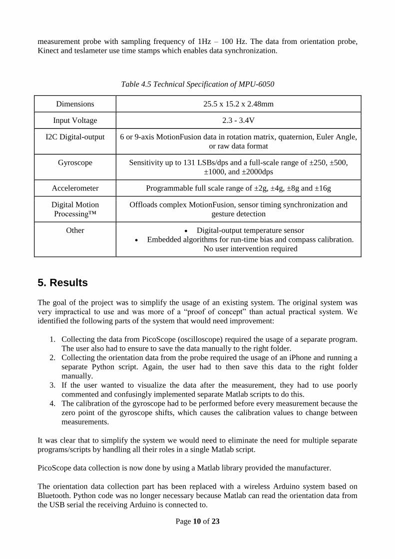
Page 10 of 23
measurement probe with sampling frequency of 1Hz – 100 Hz. The data from orientation probe,
Kinect and teslameter use time stamps which enables data synchronization.
Table 4.5 Technical Specification of MPU-6050
Dimensions 25.5 x 15.2 x 2.48mm
Input Voltage 2.3 - 3.4V
I2C Digital-output 6 or 9-axis MotionFusion data in rotation matrix, quaternion, Euler Angle,
or raw data format
Gyroscope Sensitivity up to 131 LSBs/dps and a full-scale range of ±250, ±500,
±1000, and ±2000dps
Accelerometer Programmable full scale range of ±2g, ±4g, ±8g and ±16g
Digital Motion
Processing™
Offloads complex MotionFusion, sensor timing synchronization and
gesture detection
Other Digital-output temperature sensor
Embedded algorithms for run-time bias and compass calibration.
No user intervention required
5. Results
The goal of the project was to simplify the usage of an existing system. The original system was
very impractical to use and was more of a “proof of concept” than actual practical system. We
identified the following parts of the system that would need improvement:
1. Collecting the data from PicoScope (oscilloscope) required the usage of a separate program.
The user also had to ensure to save the data manually to the right folder.
2. Collecting the orientation data from the probe required the usage of an iPhone and running a
separate Python script. Again, the user had to then save this data to the right folder
manually.
3. If the user wanted to visualize the data after the measurement, they had to use poorly
commented and confusingly implemented separate Matlab scripts to do this.
4. The calibration of the gyroscope had to be performed before every measurement because the
zero point of the gyroscope shifts, which causes the calibration values to change between
measurements.
It was clear that to simplify the system we would need to eliminate the need for multiple separate
programs/scripts by handling all their roles in a single Matlab script.
PicoScope data collection is now done by using a Matlab library provided the manufacturer.
The orientation data collection part has been replaced with a wireless Arduino system based on
Bluetooth. Python code was no longer necessary because Matlab can read the orientation data from
the USB serial the receiving Arduino is connected to.

Page 11 of 23
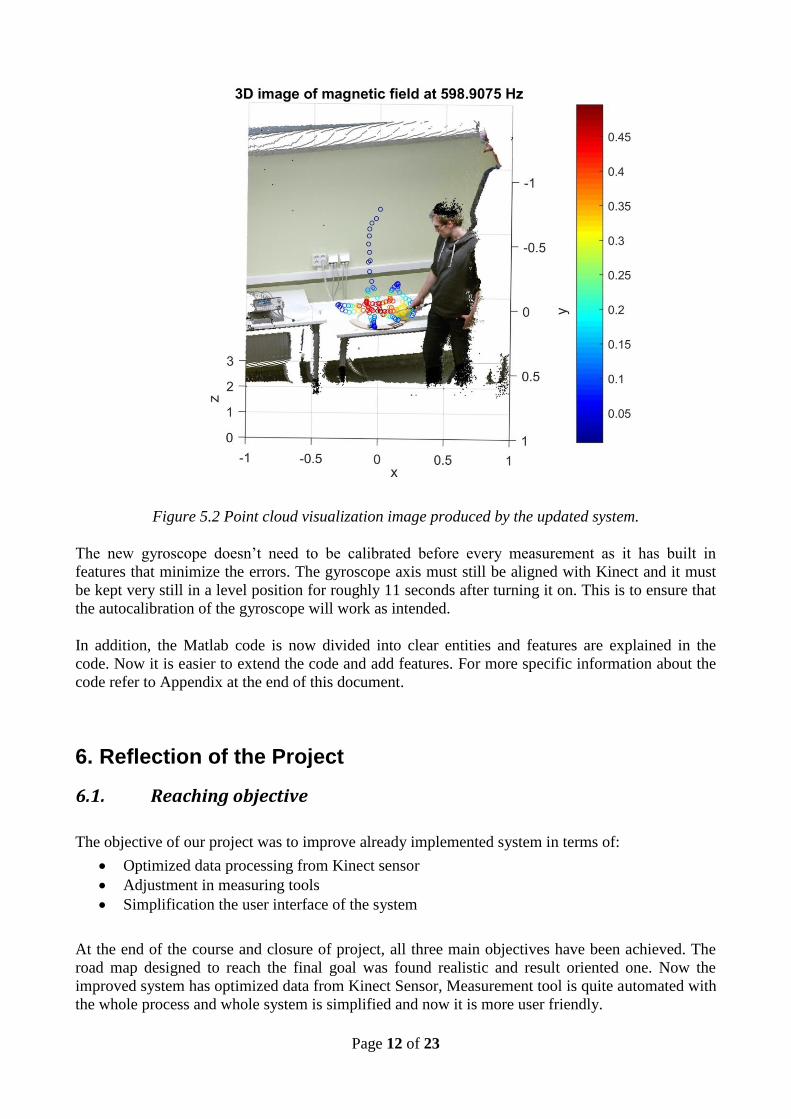
Now all the collected data is processed, visualized and saved automatically after the measurement if
the user wants it. As the original measurement system, the improved system visualizes
measurements in two ways. Because the magnetic field data contains several frequencies, the
frequency distribution is useful to show in a separate figure. The highest frequency is shown yellow
in a spectrogram that visualizes the frequency over time. The highest frequency is useful to know
because it is the frequency used in 3D image measurements, for example.
The Kinect takes two images, a depth and a color image, to create a 3D point cloud image. The
image visualizes the strength of EMF in colors from blue to red and shows the position of data
points in measurement environment.
See figures 5.1 and 5.2 for examples of the visualizations produced by the updated system.
Figure 5.1 Spectrogram image produced by the updated system.
Page 12 of 23
Figure 5.2 Point cloud visualization image produced by the updated system.
The new gyroscope doesn’t need to be calibrated before every measurement as it has built in
features that minimize the errors. The gyroscope axis must still be aligned with Kinect and it must
be kept very still in a level position for roughly 11 seconds after turning it on. This is to ensure that
the autocalibration of the gyroscope will work as intended.
In addition, the Matlab code is now divided into clear entities and features are explained in the
code. Now it is easier to extend the code and add features. For more specific information about the
code refer to Appendix at the end of this document.
6. Reflection of the Project
6.1. Reaching objective
The objective of our project was to improve already implemented system in terms of:
Optimized data processing from Kinect sensor
Adjustment in measuring tools
Simplification the user interface of the system
At the end of the course and closure of project, all three main objectives have been achieved. The
road map designed to reach the final goal was found realistic and result oriented one. Now the
improved system has optimized data from Kinect Sensor, Measurement tool is quite automated with
the whole process and whole system is simplified and now it is more user friendly.

Page 13 of 23
6.2. Timetable
The timetable was initially set for the completion of tasks was majorly remained unchanged.
Whereas some changes were made when found necessary and more realistic approach. Overall, the
schedule for each Work Package was remained as it is and didn’t require any change and Head of
WPs have concluded respective WPs within the deadline.
The break down for the work resource of each member was set according to the related task and its
schedule as well as availability of member. The work resource for each member was variable but
there is an agreement of completing 215 hours by each member during whole course. This value of
hour was obtained after subtracting compulsory hours of course which included hours related to
lectures, Business Aspect Seminar, Team Meetings and Final Gala.
The estimated time for our project was well justified. To complete 10 credits, one should cover 280
hours. As this project was extension of already executed project, so we didn’t need to struggle a lot
for the idea and feasibility analysis and moreover, related data was already available. Although,
every member estimated maximum hours for compilation of the report. But as in terms of technical
details, there was no such thing to be documented as it was already available. Overall time
management was good and there was no severity with the schedule and there were no precedence
and successors in the early part of the project and each WP team has worked and finished all related
tasks within the finish date.
6.3. Risk analysis
There were some risks listed in Project Plan and these are also given in table 6.1. These were
projected while compiling Project Plan.
Table 6.1 Risks along with severity, likelihood and counter measures
Risks Severity Likelihood Counter Measures
Lack of Theory 3 2 Proper and sufficient material will be
provided
MATLAB incompetence 4 3 Lack of MATLAB skills will be improved
with the help of Instructor
Insufficient MATLAB resource
person
3 4 Improvement and documentation of the code
as well as introduction from the responsible
person of the Matlab code at the beginning
of the integration phase
Design Error 4 2 More time has given literature and design
phase to obtain sufficient knowledge
Too Optimistic Schedule 3 2 Sufficient work hours have been allotted and

Page 14 of 23
in case work hours will not enough then
work hours related to dissemination WP will
be compensated
Unavailability of group member(s) 4 2 Workload have been divided equally and
have everyone involved in every aspect of
the project. In case of unavailability of group
member then affected workload will be
divided among rest of group members and
project plan will suffer changes.
Micro Controller incompatibilities 3 2 Micro Controller will be change
Lack of Communication 5 1 Meeting Schedule and Communication plan
will be ensured.
All the included risks were crucial and therefore countermeasures were quite clear otherwise they
may cause lagged in project schedule and also affect the goal of the project. There was no risk other
than mentioned ones appeared. During the project, some already mentioned risks appeared which
included are mentioned below.
Micro Controller incompatibilities related to design of Oscilloscope
Lack of theory
MATLAB incompetence
The countermeasures were taken and which ultimately proved to be good decisions for output of the
project. During each group meeting, risks analysis was done and tried to figure out the chances of
occurrence of the risk and if there is new risk. Usual countermeasures included plan adjustments,
finding alternative ways to complete the task and consulting the instructor of the project.
6.4. Project Meetings
According to available hours, work requirement, availability of Instructor and each member, the
schedule for meeting. The schedule for meeting is given in table 6.2
Table 6.2 Meeting hours per week.
anuary
Week 1 2hrs Week 12 2hrs
Week 2 2hrs Week 13 -
Week 3 2hrs
April
Week 14 1hr
Week 4 1hr Week 15 -
February
Week 5 - Week 16 2hrs
Week 6 1hr Week 17 -
Week 7 Exam Week
May
Week 18 2hrs
Week 8 2hrs Week 19 1hr
March
Week 9 - Week 20 1hr
Week 10 1hr Week 21 3hrs
Week 11 -

Page 15 of 23
Group Meeting with Instructor
Group Meeting without Instructor
There were total 14 meetings were planned and 2 meetings were scheduled other than planned ones
during project and both were group meeting without instructor. Therefore, there were total 16
meetings. Agenda for each meeting was shared before the meeting and were followed in almost
every meeting. Project Manager was responsible for keeping notes for each meeting.
Other than project meetings, Communication using Email and WhatsApp group made life easy for
exchange of information and overall all these factors aided towards efficient working environment
for the project. There were suggestions to have meeting on every week but our group tried to utilize
those hours in working with project because there was continuous communication among the group
members but still there should be meetings in every week to keep checking the project status.
In addition, a couple of personal meetings with instructor or single group members were arranged
when problems with the task arise. Usually this was the case when single group member needed
more information regarding some subject of the project. These meetings also proved rather useful
and usually always advanced the project.
7. Discussion and Conclusions
The course was not only based on technical capabilities but also on the team work and management
skills as well as business aspect. This assigned project was based on the previous work and the
objective was to make improvements in the system. The project requires good skills in MATLAB,
Embedded Programming and Project Management. The MATLAB section of the project was tough
as compared to other tasks and Instructor helped us a lot in development of the project. The overall
project was good. Resulting Matlab program and how to use it can be found from the Appendix
(“Project code” and “3D EMF Map User Guide).
Other than technical aspects, we learned teamwork within multicultural environment, project
planning and execution has given a valuable experience and added to our skill levels. Other than
project management, we learned how to utilize a idea into business concept and what are the
necessary phases and skills required for entrepreneurship. And how to make our idea, a market
product. Documentation also played a key role while development of the project. It helped us
documenting every happening during the course of the work. Some lessons learned that how should
documentation can be done and what are the basic parameter for the documentation.
Overall the whole project which includes Technical Part, Management, Documentation and
Business Aspect Part. Every section has given some good lessons and it will help in professional
life. During the whole course, Project Instructor given us great insight related to all the aspects of
the project.
Page 16 of 23
List of Appendixes
3D EMF Map User Guide
Notes of the 3D EMF Map code structure
Important Codes
Project Plan
Business Aspect Document
8. References
[1] L. Jukola, "Hybrid positioning and magnetic field measurement system," 2016.
Page 17 of 23
Appendix A. 3D EMF Map User Guide
This is a guide for using Matlab based 3D magnetic field measurement tool 3D EMF Map.
Operation is descripted from system setup to conducting measurements and ending the operation.
To conduct measurements, you need Xbox’s Kinect camera, PicoScope 2000 series USB
oscilloscope (2406b used here), ELT-400 Exposure Level Tester from Narda (magnetic probe), two
Arduinos with wireless communication capabilities and computer to run Matlab. Here is 3D EMF
Map operation in step by step manner:
1. Set up hardware: Connect Kinect, PicoScope and the receiving Arduino to the computer
via USB. Also connect Narda probe to PicoScope’s channels A, B and C (probe’s x-axis
cable to channel A, y-axis to channel B and z-axis to channel C) and the sending Arduino to
a battery. Make sure the gyroscope is connected to the sending Arduino and attached to the
probe. The gyroscope axis must be aligned with Kinect and it must be kept very still in a
level position for roughly 11 seconds after turning it on. Turn on Narda probe and select the
sensitivity (for example 320 uT from “Mode” button and “High” from “Range” button).
2. Start the program: First start Matlab and there navigate to
“C:\Users\zbook\Documents\Hybrid positioning and magnetic field measurement
system\Measurement”. This folder contains all relevant files for measurements.
3. Conduct measurements: To start measuring run Matlab script “EMF_3D_Map_V1.m”.
This script runs the measurements automatically from start to finish. However, there are
some phases on measurements:
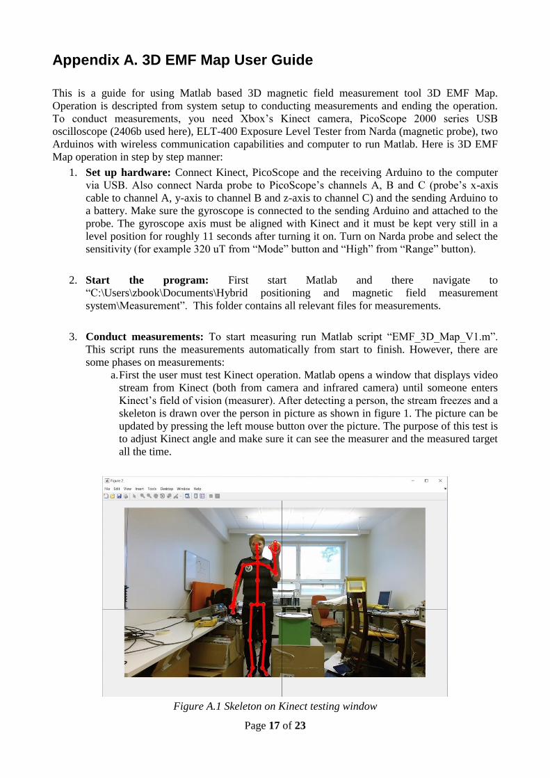
a. First the user must test Kinect operation. Matlab opens a window that displays video
stream from Kinect (both from camera and infrared camera) until someone enters
Kinect’s field of vision (measurer). After detecting a person, the stream freezes and a
skeleton is drawn over the person in picture as shown in figure 1. The picture can be
updated by pressing the left mouse button over the picture. The purpose of this test is
to adjust Kinect angle and make sure it can see the measurer and the measured target
all the time.
Figure A.1 Skeleton on Kinect testing window

Page 18 of 23
b. To start the actual measurement, click right mouse button over the picture. The
Kinect window closes and the measurement starts. A small stop button also appears
which can be used to stop the measurement.
c. After the measurement time is up or the stop button is pressed the measurement stop
and script moves to data processing.
4. Data processing: Next the data is processed. Various spectrums are calculated and data
from different devices is united. In this phase, the script asks if the user wants to visualize
the measurement results.
a. First a window shown in figure 2 appears asking if user wants to draw a spectrogram
of the measurement.
b.
Figure A.2 Spectrogram question window
b. After that a window shown in figure 3 appears asking if the user wants to show a 3D
point cloud image of the measurements.
Figure A.3 3D point cloud image question box
c. Lastly the program will ask if the user wants to save the measurement data. Data is
saved to a Matlab file called “3D magnetic field data DateAndTime.mat” where
DateAndTime is the current date and time.
4. Ending the operation: The script will automatically close all the connected devises but
there is still a small problem that the user should be aware of: Drawing the 3D point cloud
image with this script apparently jams the Kinect/Matlab. This means that Matlab still works
but new measurement cannot be conducted until Matlab is restarted. Also Matlab for some
reason must be closed from the task manager after running the measurement script.
Important notes of the system:
Kinect can only recognize measurer when his/her face is towards the camera so make sure
the measurer faces it during the measurement!
Also, there should only be one person at time on Kinect field of view when measuring
Page 19 of 23
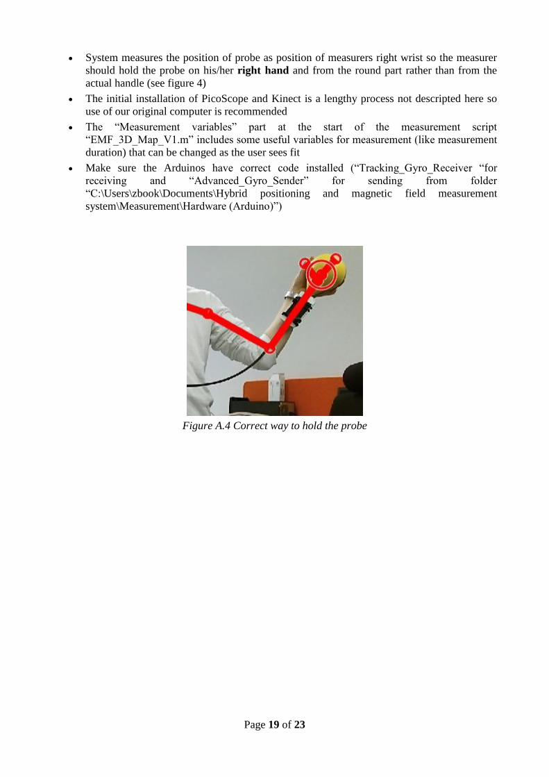
System measures the position of probe as position of measurers right wrist so the measurer
should hold the probe on his/her right hand and from the round part rather than from the
actual handle (see figure 4)
The initial installation of PicoScope and Kinect is a lengthy process not descripted here so
use of our original computer is recommended
The “Measurement variables” part at the start of the measurement script
“EMF_3D_Map_V1.m” includes some useful variables for measurement (like measurement
duration) that can be changed as the user sees fit
Make sure the Arduinos have correct code installed (“Tracking_Gyro_Receiver “for
receiving and “Advanced_Gyro_Sender” for sending from folder
“C:\Users\zbook\Documents\Hybrid positioning and magnetic field measurement
system\Measurement\Hardware (Arduino)”)
Figure A.4 Correct way to hold the probe

Page 20 of 23
Appendix B. 3D Notes of the 3D EMF Map code structure
Original code for this 3D magnetic field measurement device included Matlab, Python and Arduino
codes and an additional program for PicoScope that had to be ran separately. System operation also
included a lot of manual phases like starting programs and saving data. However, with this new
improved system only a single Matlab script is used to do all the measurements, data processing,
visualization and data capture. This makes the system much more user friendly and easier to adopt
for new users.
Even though the system is now easier to use it is still rather complex to modify. The main Matlab
code for example has around 800 lines of code and there are also couple of additional functions it
uses. Another reason for complexity is that the system uses internal methods of Kinect and
PicoScope through Matlab and their operation might be little tricky to figure out. However, the code
has been commented quite well which improves the learning process even though it still is rather
time consuming. This document also contains a brief explanation of the basic structure and some
notes of the system code to help with any future improvement of the system. For instructions to use
the measurement system refer “3D EMF Map User Guide”.
Appendix C. Important codes
Main script “EMF_3D_Map_V1.m”
The main code of the 3D EMF Map magnetic field measurement system is a Matlab script
“EMF_3D_Map_V1.m”. This script basically handles the whole measurement process and provides
a simple user interface. The code is divided to different blocks by measurement process phases. The
phases are: Hardware setup, Kinect test, Measurement, Data processing and Ending operation.
These blocks are also divided to smaller sub-blocks depending on their function. The most common
division is done by operating hardware (Kinect, PicoScope or Arduino). Usually the largest sub-
blocks deal with PicoScope operation.
To understand the code we briefly introduce the measurement operating principle. The
measurement system contains three measuring devices: Kinect, Narda’s magnetic probe and
gyroscope connected to Arduino. Kinect measures the position of the probe in 3D space, probe
measures strength of magnetic field and gyroscope orientation of the probe. In data processing part
different measurement quantities are tied together and used with each other.
Then back to the actual code. First block in the script simply connects each three devices (Kinect,
probe through PicoScope and Arduino) to Matlab using their internal methods (Kinect: Mex files,
PicoScope: dll libraries and Arduino simply uses serial connection). Many variables for
measurement are also set in this block. More information of devices internal operation can be found
on their respective documentation.
Second block uses only Kinect. In this block we test Kinect operation by showing video stream
from the device. Block has one main while-loop that updates the picture and checks if there is a
person in the Kinect field of view. When person is detected the automatic frame update stops and
Page 21 of 23
next frame is shown only after clicking left mouse button as long as the person remains in the field
of view. To stop the test and start measurement right mouse button must be pressed.
Third block contains the actual measurement loop. Most of the loop contains PicoScope operation
for getting values for magnetic field (huge number of measurements with each loop iteration). At
the end side of the loop there are separate smaller sub-blocks for Kinect measurement (records the
position of users right wrist as x,y,z coordinate to an array) and Arduino/gyroscope measurement
(orientation as x,y,z value to an array). It should be noticed that there will be same number of
Kinect and Arduino measurements but several times more probe measurements. Therefore, the
single position and orientation corresponds to block of magnetic field values (certain time period)
since Kinect and Arduino are considerably slower measurement devices. This measurement loop
stops only when set time has passed or the generated stop button is pressed.
Fourth block contains all the data processing. First we get all the final probe data from PicoScope.
Then in the next sub-block we calculate a spectrum for each position-orientation pair from their
corresponding block of probe data with function “movingSpectrum”. After that the rest of the block
is basically visualization of data as spectrogram or 3D point cloud image from Kinect. There are
also additional visualization possibilities for raw data that are commented out but can be used if
needed. Last part of the block is for saving the measurement data for later use. System saves the raw
magnetic field data of each probe channel (channelAFinal, channelBFinal, channelCFinal), position
data from Kinect (hand_r), orientation data from Arduino (position), time points for each
position/orientation measurement point (time_f), measurement starting time (Tstart), point cloud for
later visualization (ptCloud) and the spectrum arrays of the measurement mentioned earlier
(FsignalA0, FsignalB0, FsignalC0). Data is saved to file which name includes measurement date
and time.
The last block in the script only disconnects all the devices and deletes the device objects.
movingSpectrum
movingSpectrum is a Matlab function used to calculate spectrum for each position/orientation pair
or time point. Single spectrum is calculated from part of final magnetic field data using the
measurement time points (time_f in main code). Basically function takes probe data with the size of
one time step and calculates the spectrum with fft then moves on by length of time step and
calculates the next spectrum. This continues until all probe data is dealt with. There is also option of
choosing the time window used in spectrum calculations. Finally the function returns an array that
has all the calculated spectrums (Fsignal) and some other values like down sampled signal.
Tracking_Gyro_Receiver
Arduino code for receiving Arduino. This code includes receiving wireless transmission from the
transmitting Arduino with the gyroscope. In addition the code sends the received data to computer
via serial port from where Matlab can later read it.
Advanced_Gyro_Sender
Arduino code for sending Arduino with the gyroscope. This code includes operating the gyroscope
and wireless data transmission to the receiving Arduino. Basically it sets up the gyroscope and
Page 22 of 23
wireless link and starts operation and transmission if no error occurs. Gyroscope operation requires
that correct library files are present as mentioned at the beginning of code.
Other files
System runs with these codes but devices use several internal methods when to run in Matlab.
Kinect uses Mex files to convert operation from C++ to Matlab (originate from Kinect SDK),
PicoScope uses dll libraries and parts from PicoSDK, PicoScope Support Toolbox and PicoScope 6
program and Arduino uses some external libraries. Therefore, using the measuring system on other
new computers requires quite much installation and struggling. More information of these can be
found from kin2-user-guide (Kinect) and picotech’s websites (PicoScope).
Faults and improvement suggestions
Even though measuring system works and is much easier to use compared to before there are still
some faults. First of all Kinect freezes for some reason after the measurement. More precisely you
can only take one point cloud image with it and then it throws an error when trying to take new one.
This prevents consecutive measurements and Matlab needs to be restarted between measurements.
Even though Matlab does not freeze the freezing of Kinect prevents closing Matlab normally and
also deleting some variables. Therefore, Matlab must be closed using task manager.
Other regrettable issue was orientation measurement implementation. Communication between
Matlab and Arduino works on separate code (see script “Arduino_to_Matlab” for example) but for
some reason the same communication won’t work when implemented into EMF_3D_Map_V1.
This issue is somewhat severe and was noticed too late to fix. Apparently “Measurement” loop in
the code (sub-block “Arduino measurement”) tries to read serial port infinitely and measurement
gets stuck there.
Other minor issues that affect usability more than actual operation include gathering variables to
one place and otherwise making parameters easier to change. At the moment almost all parameters
like PicoScope sampling frequency and range must be manually changed from somewhere (usually
set up block) from the code using device’s own syntaxes. Some sort of control window would be
ideal for changing the parameters.
Another minor issue is the length of the code. The main script is over 800 lines long and some of
the parts could be implemented as their own functions. The main reason why most of the code is in
single script is that devices need to use their internal methods to operate. Therefore, dividing code
to functions would require passing considerable amount of input and output variables. Though this
issue does not affect the operation of the system it could make the system simpler and more
manageable.
One of the biggest issues during the coding process of the measurement system was the
implementation of parallel measurement of devices. Ideally all the measuring tools would run in
parallel so that the measurement would be conducted continuously at the same time. However,
implementing this on Matlab proved rather difficult. Matlab does not offer right tools for running
measuring loops in parallel or swift interaction with different parallel elements. Although Matlab
does have some parallel processing capabilities (parpool, spmd) they are more useful for processing

Page 23 of 23
existing data and do not offer any possibility for interaction with the user. Even worse problem was
that Matlab’s parallel processing severs the connection to hardware devices. Thus, the processing in
our system is not actually parallel but all three measurements are done in series during each loop
iteration. This still gives correct values but might affect the phase of magnetic field measurement.
One future prospect could be implementing parallel measurement with Simulink or using other
coding languages.
The system also still needs more testing. There are many situations where the system might act
unexpectedly like when the Kinect loses sight of the measurer or when there are more than one
person in Kinect’s field of view and many others.
Last improvement could be implementing memory allocation of the system so that it can measure as
long as needed without any set maximum measuring time. This could make measurement smoother
since now best way to do this is to set measuring time very long and simply push stop button when
user wants to quit.