final report residential trip generation: · pdf fileabstract residential trip generation...
TRANSCRIPT

FINAL REPORT
RESIDENTIAL TRIP GENERATION: GROUND COUNTS VERSUS SURVEYS
Jared M. Ulmer Graduate Research Assistant
Arkopal K. Goswami
Graduate Research Assistant
John S. Miller, Ph.D., P.E. Senior Research Scientist
Lester A. Hoel, D. Eng.
L.A. Lacy Distinguished Professor of Engineering and
Faculty Research Scientist
Virginia Transportation Research Council (A Cooperative Organization Sponsored Jointly by the
Virginia Department of Transportation and the University of Virginia)
In Cooperation with the U.S. Department of Transportation
Federal Highway Administration
Charlottesville, Virginia
June 2003 VTRC 03-R18

ii
DISCLAIMER
The contents of this report reflect the views of the authors who are responsible for the facts and the accuracy of the data presented herein. The contents do not necessarily reflect the official views or policies of the Virginia Department of Transportation, the Virginia Transportation Research Council, or the Federal Highway Administration. This report does not constitute a standard, specification, or regulation.
Copyright 2003 by the Commonwealth of Virginia.

iii
ABSTRACT
Residential trip generation rates, defined herein as the total number of vehicle trips per household during a 24-hour period, are a fundamental component of transportation planning. When agencies have different estimates of these rates for the same metropolitan area, the cost of the planning process increases since agencies must collect additional field data. To investigate discrepancies in these rates, residential trip generation rates based on four sources were compared: (1) ground counts collected by the Virginia Transportation Research Council (VTRC) at nine suburban neighborhoods, (2) household surveys distributed to the same neighborhoods, (3) national trip generation rates published by the Institute of Transportation Engineers (ITE), and (4) rates derived from the trip generation component of Virginia Department of Transportation (VDOT) regional urban travel demand models.
For neighborhoods composed solely of single-family detached homes, the average residential trip generation rate was 10.8 based on VTRC ground counts and 9.2 based on VTRC household surveys. Although underreporting of trips on written questionnaires may have contributed to this disparity, these rates were not significantly different at the 95 percent confidence level. Further, ground counts collected by VTRC and ground count rates reported by ITE were not significantly different.
However, rates based on VTRC household surveys and those derived from VDOT regional models were significantly different when the VDOT rates were based on person trips rather than vehicle trips. This disparity resulted even though the person trips predicted by the VDOT long-range model were converted to vehicle trips using average automobile occupancies. The implication, therefore, is that when a data source gives the number of “vehicle trips per household” it is important to know if vehicle trips were measured directly or were calculated from person trips.
When a consistent method of determining trip generation rates is used, the differences in rates between neighborhoods are explained by the large and random variations that are fundamental to trip generation studies. Accordingly, when a precise trip generation rate is required to forecast travel from a single neighborhood, the rate should be determined from field data if possible. When a trip generation rate is required for a group of neighborhoods (as is often the case with subarea studies), the average rate should be presented as part of a confidence interval as has been done in this study. For example, ground count data collected in this study for a set of seven neighborhoods of single-family detached homes produced a mean trip generation rate of 10.81, with a range of 9.4 to 12.2 vehicle trips per dwelling unit at the 95 percent confidence level. The ITE mean rate based on 348 neighborhoods was 9.57 vehicle trips per dwelling unit. As the number of neighborhoods increases, the confidence interval for the mean rate will decrease.
Variation among the four types of rates is greater that the variation in rates from one location to another. This result suggests that when, as a cost savings measure, trip generation rates are based on previous studies (i.e., VTRC or ITE) rather than new field data, the selected rates should be from the same source. Consistency can be improved by following the data collection methodology described in Appendix A.
FINAL REPORT
RESIDENTIAL TRIP GENERATION: GROUND COUNTS VERSUS SURVEYS
Jared M. Ulmer Graduate Research Assistant
Arkopal K. Goswami
Graduate Research Assistant
John S. Miller, Ph.D., P.E. Senior Research Scientist
Lester A. Hoel, D. Eng.
L.A. Lacy Distinguished Professor of Engineering and
Faculty Research Scientist
INTRODUCTION
Residential trip generation, i.e., the number of vehicle trips or person trips attributed to a group of households in a single geographic location, is a fundamental element of the transportation forecasting process. Three principal categories of transportation planning studies, i.e., long-range regional studies, midrange subarea studies, and short-range site impact studies, use residential trip generation rates. These studies use two methods to define such rates: ground counts and household surveys. In this study, trip generation refers to the number of vehicle trips per dwelling unit unless stated otherwise.
Alternative Definitions of a Residential Trip Generation Rate
A regional study forecasts person trips by different trip purposes for a metropolitan area with a planning horizon of 10 to 30 years. Travel forecasts are based on a four-step modeling process consisting of trip generation, trip distribution, mode choice, and traffic assignment. Household survey data and socioeconomic characteristics such as income, automobile ownership, and family size are used to determine the number of person trips generated per household, and then these person trips are converted to vehicle trips using appropriate automobile occupancy values. Trip generation rates reported for the Washington, D.C., regional model for two-vehicle suburban single-family households are 5.9 vehicle trips per dwelling unit based on the following trip purposes:1,2
• 2.36 work trips per household • 0.63 shopping trip per household

2
• 2.30 other trips per household • 0.60 nonresident trip per household.
A subarea study focuses on a subset of a metropolitan region in greater detail than the long-range regional study. The relative advantage of subarea studies is reduced computational requirements and data collection costs; the caveat is that the transportation improvements under consideration will affect only the location being evaluated and not the entire region.3 The regional model is the starting point: a cordon is drawn around the subarea of interest and the trip generation, distribution, and assignment data applicable to that subarea are extracted. Methodologically, the literature indicates that the subarea approach is similar to the regional approach: the trip generation, trip distribution, and traffic assignment steps are replicated for the subarea and modified as necessary to match modeled and observed traffic volumes.4
A site impact study estimates trip generation rates as the number of vehicle trips that will result from a specific new land use development such as a shopping center, restaurant, or residential neighborhood. The time frame until the build-out of the site for traffic forecasting is usually 3 to 5 years. Unless local data are collected, residential trip generation rates are usually taken from the Institute for Transportation Engineers’ (ITE) Trip Generation.5 For example, ITE gives an average 24-hour trip rate of 9.57 vehicle trips per single-family detached dwelling unit in a suburban area not served by transit, an average based on 348 individual ground count studies in the United States.
Figure 1 illustrates the relative size of each study. The size of a subarea is much smaller than a region; for example, the North Jersey regional model represents 13 counties and more than 200 municipalities, whereas the Northwest Bergen County (subarea) model represents one fourth of one county and 16 municipalities.4 In contrast, a subarea is much larger than the typically homogeneous location studied under a site impact analysis. Table 1 summarizes the distinguishing features of these three kinds of studies.
Figure 1. Variations in Geographical Scope for the Three Categories of Planning Studies
3
Table 1. Typical Characteristics of the Three Categories of Planning Studies 3,4,7
Characteristic Regional Study Subarea Study Site Impact Study
Definition of residential trip generation rate
Usually total number of person trips per household, stratified by trip purpose, income, and automobile ownership and resident versus nonresident*6
Vehicle trips or person trips per day per household
Total number of vehicle trips per household made by residents and nonresidents
Data source Household surveys
Ground counts or data extracted from regional model**
Ground counts
Geographical scope Metropolitan region consisting of 2 to 3 thousand zones
Few zones of regional study subdivided into many subzones
One transportation analysis zone or less
Planning horizon 20 years 3 to 20 years Less than 3 years *Although person trips are typically the basis, in at least the Northern Virginia District, VDOT has used vehicle trips. ** In some instances, VDOT conducts tube counts at specific subdivisions rather than using the regional model.
Challenges to Comparing Different Residential Trip Generation Rates
In urban areas such as Northern Virginia, the Virginia Department of Transportation (VDOT) often performs subarea studies. For example, for a typical suburban household represented in the Northern Virginia portion of the regional model used by the Metropolitan Washington Council of Governments (MWCOG), the current trip generation rate is 9.79 vehicle trips per dwelling unit, which does not match the 12 trips per dwelling unit that VDOT has reported at some residential developments in Northern Virginia.7
Further, minutes from the Fall 2000 meeting of the Virginia Transportation Research Council’s (VTRC) Transportation Planning Research Advisory Committee, released on January 22, 2001, stated that “the traditional 4-step planning process used in the development of regional transportation models generally results in about 5 or 6 trips/d.u. if the zonal trip forecasts are divided by the number of dwelling units.” Assuming these “5 or 6 trips” per dwelling unit denote vehicle trips, there is a wide disparity between the regional model rate and the VDOT rate of 12 vehicle trips per dwelling unit. Should, however, the “5 or 6 trips” per dwelling unit denote person trips, their conversion to vehicle trips would yield an even lower number of vehicle trips for the regional model and, as a consequence, an even greater disparity between the VDOT rate and the regional model rate.
As a result of such discrepancies, VDOT collects new trip generation data each time a subarea study is performed instead of using the lower MWCOG value. To reduce the financial costs associated with collecting these new data, VDOT needs to understand why the two rates are different.
The literature is helpful but not definitive in this regard. The broader question of how to apply regional information from the regional model to subarea studies has been posed previously; for example, Pedersen and Samdahl noted that the intensity of land uses should be

4
examined when a trip generation rate is transferred from the regional to the subarea model.8 Researchers have also looked at using the detailed updated subarea information to improve the resultant regional model: Cervero found in one particular study that the effects were negligible but warned that his findings might not apply elsewhere, whereas Winslow et al. suggested that subarea studies and regional models should be calibrated at the same time.4,9
At the outset of this study, four potential reasons for the variation in residential trip generation were identified:
1. Differences in trip rate definitions, given that site impact analysis techniques based on ground counts include all vehicle trips whereas a rate reported from the regional model, based on household surveys, may not necessarily include truck trips or external vehicle trips. Such trips are undoubtedly included in the regional model but may or may not necessarily be included when a household trip generation rate is reported. Similarly, the person trip versus vehicle trip distinction may be problematic, as was found to be the case with some of the sites used in this study where for at least one region the VDOT long-range model is based on vehicle trips and in other regions the long-range model is based on person trips.
2. Geographical differences, e.g., residents in the suburban area of Richmond may or
may not show different rates from residents in the suburban area of Hampton Roads.
3. Law of averages. Even in the same metropolitan area, the regional model represents a regional average whereas the site impact analysis is comparable to an individual observation.
4. Differences in the proportion of trips generated by residents and nonresidents. Since
the regional model differentiates between these two categories in the form of productions and attractions, differences in the proportion of trips made by residents could affect the resulting trip generation rate.
These four reasons can apply even if the data are collected from homogeneous neighborhoods at the same time. If data are not collected from homogeneous areas, then other reasons may explain differences in rates. Among these are temporal or seasonal differences (e.g., if the regional model was calibrated several years earlier or the ground counts were performed in the summer), land use variation (e.g., usually neighborhoods in high-density locations tend to have a greater proportion of walking or transit trips), or socioeconomic differences (e.g., higher automobile ownership is often indicative of additional travel).
PURPOSE AND SCOPE
The purpose of this project was to investigate the differences between trip generation rates based on ground counts and those based on household surveys. With a rational basis for subarea trip generation and a better understanding of the reasons variation exists in trip

5
generation rates, it will become clearer which residential trip generation rate is appropriate for VDOT to use in subarea studies.
Accordingly, there were four objectives of this study:
1. Determine whether there are statistically significant differences between mean ground count trip rates and mean household survey trip rates as collected by VTRC.
2. Determine whether there is statistically significant geographic variation in these
VTRC residential trip rates.
3. Compare VTRC field data with average rates provided by ITE and those estimated by VDOT in regional studies.5 (Such comparisons indicate the suitability of nationally or regionally published average rates to represent rates observed at individual neighborhoods.)
4. Determine whether the proportion of trips generated by residents and nonresidents is
statistically different between neighborhoods and/or between VTRC ground count and household survey trip generation rates.
The scope of this study was limited in four key ways: 1. Three neighborhoods were studied in each of three Virginia regions during a 22-
month period. The regions were Central Virginia (Albemarle County and the City of Charlottesville), Northern Virginia (Fairfax County and Loudoun County), and Hampton Roads (the City of Suffolk).
2. Residential neighborhoods that contained between 90 and 300 dwelling units and no
other land uses were targeted. In some cases neighborhoods with fewer than 90 dwelling units were used when obtaining a suitable site was difficult.
3. Trip length, vehicle speed, and vehicle occupancy were not measured.
4. Analysis of trip generation rates was limited to data for household surveys and
ground counts. Techniques for modifying such rates, which is part of calibrating a regional model, were not part of this effort.
METHODS AND DEFINITIONS
Four categories of trip generation rates were used:
1. VTRC ground count trip rates, i.e., the total number of vehicle trips per household entering and exiting a residential development based on VTRC observations of a particular neighborhood.

6
2. VTRC household survey trip rates, i.e., the total number of vehicle trips per household based on surveys developed by VTRC.
3. ITE ground count trip rates, i.e., the total number of vehicle trips per household
entering and exiting a residential development based on national observations.5
4. VDOT household survey trip rates, i.e., the total number of vehicle trips per household made by neighborhood residents based on the trip generation step of the appropriate VDOT regional model For Northern Virginia, the regional model reports vehicle trips directly. For the Charlottesville and Hampton Roads regional models, person trips are reported. The person trips were then converted to vehicle trips by the investigators using appropriate automobile occupancy rates.
There are differences in the trip rates. The ITE ground count trip rates and the VTRC
ground count trip rates differ only in one regard: the ITE rates are based on a national average whereas the VTRC rates are based on data collected at specific residential developments.5 Similarly, the VDOT household survey trip rates and the VTRC household survey trip rates differ primarily in that the former is an average for an entire metropolitan area whereas the latter is for at a specific development.
Data Collection
Ground counts and household surveys were conducted at residential neighborhoods in Central Virginia, Northern Virginia, and Hampton Roads using the following procedure.
1. Manually record license plate numbers, and calculate VTRC ground count trip rates.
2. Design and distribute a household trip survey, and calculate VTRC household survey trip rates.
3. Determine the ITE ground count trip rates for each development using ITE Trip Generation.5
4. Determine the VDOT household survey trip rates based on the trip generation component of the VDOT regional model for each development; neighborhood-specific socioeconomic data; and for Hampton Roads and Charlottesville, available automobile occupancies.
5. Document helpful changes to the data collection procedures in Appendix A. For
example, problems at one neighborhood forced the investigators to discard the data and restudy the neighborhood. Appendix A contains the revised data collection procedures that were found helpful for avoiding such mistakes.

7
Data Analysis Four analytical tasks, corresponding to the four objectives, were performed:
1. Determine whether mean VTRC ground count trip rates and mean VTRC household survey trip rates are statistically different.
2. Determine whether there is a statistically significant geographic variation in the mean
VTRC residential trip rates.
3. Compare VTRC field data with average rates provided by ITE and those estimated by VDOT in regional studies.5
4. Determine whether the proportion of trips generated by residents is statistically
different between neighborhoods and/or between VTRC trip generation rates. Difference Between VTRC Ground Count Trip Rates and Mean VTRC Household Survey Trip Rates
Figure 2 illustrates that for a specific neighborhood, the VTRC ground count trip rate is an individual observation, whereas the VTRC household survey trip rate is an average observation. Determining whether an individual value and an average value are “different” is an unusual question; thus, two statistical tests were conducted.
1. For each neighborhood, determine whether the single VTRC ground count trip rate falls within the 95 percent confidence interval associated with the mean VTRC household survey trip rate. The 95 percent confidence interval for the mean VTRC household survey trip rate is given as
surveys of numberdeviation standardsurvey rate trip survey household VTRC Mean )(96.1± (Eq. 1)
Using Figure 2 as a guide, the application of Eq. 1 for Schooner Cove is based on the 50 surveys returned by residents of that neighborhood, whereas for Burnetts Mill and Bennetts Creek Landing, the values are 31 and 45, respectively. This statistical test is useful but is not perfect simply because it is comparing a single point value, i.e., the mean ground count rate, to a range of values reflecting VTRC survey rates. The test does, however, intuitively convey whether these two entities are more likely to be similar or different.
2. For each metropolitan area, determine whether the mean VTRC ground count trip
rate is significantly different from the mean VTRC household survey rate. If the answer to Eq. 2 is yes, then there is a significant difference between the VTRC ground count trip rates and the VTRC household survey trip rates.

8
22
?ghh g
SSIs U U T
n n− > + (Eq. 2)
In Eq. 2, U and S indicate the mean and standard deviations for the trip rates corresponding to the ground count method (g) and the household survey method (h); n is the number of neighborhoods for each metropolitan area. Using Figure 2 for the Hampton Roads metropolitan area, there are n = 3 neighborhoods where each neighborhood contributes one ground count rate (to obtain Ug and Sg) and one mean household survey rate (to obtain Uh and Sh). This approach means that regardless of the number of surveys received, each neighborhood carries the same weight when computing a mean household survey rate for the metropolitan area. For large samples, 1.96 may be used in lieu of T; for small sizes, however, the T statistic that corresponds to 2n-2 degrees of freedom at the 95 percent confidence level would be used, which in this case with n = 3, 2.78 would be used.
Figure 2. VTRC Ground Count and Household Survey Data for Hampton Roads Metropolitan Area Geographic Variation in Mean VTRC Residential Trip Rates
Two statistical methods were used to assess the effect of location while controlling for the differences in trip rate methods.
1. Compare mean household survey rates for each neighborhood using an approach
similar to Eq. 2 but described in Eq. 3, where nx and ny designate the number of households in neighborhood x and y, respectively.
22
?yxx y
x y
SSIs U U T
n n− > + (Eq. 3)

9
2. Conduct an analysis of variance (ANOVA) using the VTRC ground counts for each neighborhood and ascertain whether there are significant differences when stratifying these counts by metropolitan area. This ANOVA is then repeated using the mean VTRC household survey rate for each neighborhood.
Comparison of VTRC Field Data With Average Rates Provided by ITE and Those Estimated by VDOT in Regional Studies The VTRC ground count rates may be compared to the nationally published ITE ground count rates using two statistical approaches:5
1. Compare the VTRC ground count rates and the ITE ground count rates using Eq. 3. 2. Compare the confidence intervals for individual observations for the VTRC ground
count rates and the ITE ground count rates. The 95 percent confidence interval for an individual neighborhood observation is
)(96.1 deviation standardcount ground rate count ground VTRC Mean ± (Eq. 4) This confidence interval for an individual observation is much wider than the confidence interval used for the mean, which was
odsneighborho of numberdeviation standardcount ground rate count ground VTRC Mean )(96.1
± (Eq. 5)
The VTRC household survey rates may be compared with the VDOT regional model
rates using an approach similar to that described in Eq. 1, where one visually inspects whether the VDOT regional model rate falls within the 95 percent confidence interval for the mean VTRC household survey rate. Differences in Proportion of Trips Generated by Residents Between Neighborhoods and/or Between VTRC Trip Generation Rates
Two tests were used. First, ANOVA was used to determine whether there was significant variation among neighborhoods. Second, because of uncertainty associated with some of the data collection procedures, confidence bounds that account for experimental error associated with the ground counts were developed in accordance with procedures described in Appendix B. Confidence intervals that describe the statistical variation were developed in accordance with Eq. 6, where the 95 percent confidence intervals associated with the proportion of trips made by residents are given as

10
(1 )1.96
proportion proportionproportionsample size
−± (Eq. 6)
RESULTS
Field Data Collection Procedures and Data Overview
Ground count data, household survey data, and socioeconomic data were collected from nine sites in three metropolitan areas as denoted in Table 2. One neighborhood in Northern Virginia, i.e., Westport, was surveyed twice to determine the number of trips attributable to residents; accordingly, only data from the second visit are reported. Two Central Virginia neighborhoods, i.e., Montvue and Terrell, had an insufficient number of returned surveys to develop reliable trip rates based on household surveys. Survey response rates ranged from 13 to 56 percent, and the three neighborhoods with the lowest response rates were located in Northern Virginia.
Data collection errors were reduced by adhering to the revised data collection guidelines
shown in Appendix A. For example, initially between 4.4 and 10.8 percent of the vehicles could not be definitively classified as belonging to neighborhood residents versus nonresidents. A slight change in the data collection procedure (allowing only one license plate per line on the data collection form as shown in Figure A6) resulted in a decrease in the undetermined plates to 0.4 percent at one site. For reasons such as this, the data collection procedures that reduce data collection uncertainty to the minimum observed in this study are provided in Appendix A.
Table 2. Survey Response Rate for Each Neighborhood
Neighborhood
Metropolitan Area
No.
Households
No. Surveys
Received
Neighborhood Survey Response
Rate (%) Schooner Cove Hampton Roads 90 50 56 Burnetts Mill Hampton Roads 111 31 28 Bennetts Creek Landing Hampton Roads 135 45 33 Westport Northern Virginia 167 22 13 Fair Ridge Northern Virginia 225 38 17 Foxlee Northern Virginia 90 25 28 Johnson Village Central Virginia 225 77 34 Terrell Central Virginia 29 16 55 Montvue Central Virginia 38 14 37 Average Household Response Rate (total surveys received divided by total households) 29 Average Neighborhood Response Rate (average of neighborhood survey response rates) 35

11
Comparison of VTRC Ground Count Trip Rates and Household Survey Trip Rates
Table 3 shows the mean VTRC residential trip generation rates for each neighborhood. Two of the neighborhoods, Johnson Village and Fair Ridge, had townhomes or duplexes. Using the VTRC ground counts shown in Table 3, the two neighborhoods with townhomes and duplexes produce statistically different trip generation rates; further, ITE has different classification systems for these types of neighborhoods as opposed to those that have only single-family detached dwelling units.5 Thus, the average trip rate for this study was computed with and without these two sites, as shown at the bottom of the table.
Using the VTRC household survey data and Eq. 1, 95 percent confidence intervals for the mean VTRC household survey rate were computed for each of seven neighborhoods and were compared to the corresponding VTRC ground counts. Table 4 illustrates the resulting confidence intervals for each neighborhood and compares these with the VTRC ground count rates. The results indicate that ground counts are subsumed within confidence intervals for five of the seven sites. These test results suggest that in most cases no significant difference between the ground count rates and the household survey rates exist, but when they do, the ground count trip rate is greater than the household survey rate.
Eq. 1 is a reasonable approach for testing significant differences in trip rates, but it is
limited because a mean value based on household surveys is compared with a single point value based on ground counts. Accordingly, Eq. 2 was used to test for differences between ground counts and household surveys within the metropolitan areas of Hampton Roads and Northern Virginia. In each region, the results showed no significant difference between ground counts and household surveys, with confidence levels of 82 percent and 26 percent for Hampton Roads and Northern Virginia, respectively.
Table 3. Mean VTRC Residential Trip Generation Rates
Neighborhood
Metropolitan Area
VTRC Ground Count Rate
Mean VTRC Household Survey Rate
Schooner Cove Hampton Roads 11.20 7.60 Burnetts Mill Hampton Roads 12.32 7.86 Bennetts Creek Landing Hampton Roads 7.13 7.33 Westport Northern Virginia 10.18 12.37 Fair Ridgem Northern Virginia 6.20 6.48 Foxlee Northern Virginia 10.70 10.60 Johnson Villagem Central Virginia 7.92 7.98 Terrell Central Virginia 13.14 * Montvue Central Virginia 11.02 * Mean (of all sites) 9.98 8.60 Coefficient of variation (of all sites) 23.83 24.29 Mean (without townhome sites) 10.81 9.15 Coefficient of variation (without townhome sites) 17.65 24.32
m Site includes townhomes or duplexes. *VTRC household survey response rate could not be determined due to an insufficient number of returned surveys.
12
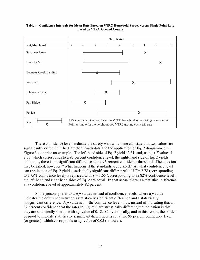
Table 4. Confidence Intervals for Mean Rate Based on VTRC Household Survey versus Single Point Rate Based on VTRC Ground Counts
These confidence levels indicate the surety with which one can state that two values are significantly different. The Hampton Roads data and the application of Eq. 2 diagrammed in Figure 3 comprise an example. The left-hand side of Eq. 2 yields 2.61, and, using a T value of 2.78, which corresponds to a 95 percent confidence level, the right-hand side of Eq. 2 yields 4.40; thus, there is no significant difference at the 95 percent confidence threshold. The question may be asked, however: “What happens if the standards are relaxed? At what confidence level can application of Eq. 2 yield a statistically significant difference?” If T = 2.78 (corresponding to a 95% confidence level) is replaced with T = 1.65 (corresponding to an 82% confidence level), the left-hand and right-hand sides of Eq. 2 are equal. In that sense, there is a statistical difference at a confidence level of approximately 82 percent.
Some persons prefer to use p values instead of confidence levels, where a p value
indicates the difference between a statistically significant difference and a statistically insignificant difference. A p value is 1 – the confidence level; thus, instead of indicating that an 82 percent confidence that the rates in Figure 3 are statistically different, the indication is that they are statistically similar with a p value of 0.18. Conventionally, and in this report, the burden of proof to indicate statistically significant differences is set at the 95 percent confidence level (or greater), which corresponds to a p value of 0.05 (or lower).

13
Figure 3. Computation of Confidence Levels
Geographic Variation within the VTRC Residential Trip Generation Rates
Visual inspection of Table 4 indicates that the confidence intervals for most sites based
on household surveys have substantial overlap. Application of Eq. 3 results in three distinct findings pertaining to residential trip generation rates as reflected in Table 5:
• There is no significant difference in trip rates among the five neighborhoods of Fair Ridge, Bennetts Creek Landing, Schooner Cove, Burnetts Mill, and Johnson Village.
• There is no significant difference between the two neighborhoods of Foxlee and
Westport.
• Much of the significant differences among these locations can be attributed to the Westport neighborhood. In other words, had Westport not been studied, then all of the comparisons, except for that of Foxlee/Fair Ridge, would have shown insignificant differences.
Table 5. Test of Significant Differences Among Neighborhoods According to VTRC Household Surveys

14
In sum, variation in the mean household survey rates was usually not significant when individual neighborhoods were compared to one another. This finding was confirmed by an ANOVA that looked at differences among the metropolitan areas of Hampton Roads, Northern Virginia, and Central Virginia. With confidence levels of 26 and 51 percent for VTRC ground counts and VTRC household surveys, respectively, there were no statistically significant differences among residential trip generation rates when stratified by metropolitan area. Removal of Johnson Village, which was the only Central Virginia neighborhood shown in Figure 4, yielded insignificant confidence levels of 55 and 72 percent, respectively. A single-factor ANOVA rather than a two-factor ANOVA was used to keep reported confidence levels consistent with Eqs. 1 through 3.
Comparison of VTRC Field Data and National (ITE) Trip Rates
Confidence intervals for the mean VTRC ground count rates based on the seven neighborhoods with only single-family detached dwelling units are shown in Table 6. The last two lines of Table 6 show 95 percent confidence bounds for an individual neighborhood’s rate using Eq. 5. An interpretation of the results shown in Table 6 is as follows:
• Assuming an infinitely large sample of neighborhoods similar to those studied, the researchers are 95 percent confident that the true mean residential trip generation rate is between 9.40 and 12.23 trips per dwelling unit.
• Assuming an infinitely large sample of neighborhoods similar to those studied, the
researchers are 95 percent confident that an individual neighborhood will have a trip generation rate between 7.07 and 14.55 trips per dwelling unit.
Table 6 also shows the resultant 95 percent confidence intervals for a mean value and an
individual neighborhood based on the data in ITEs Trip Generation.5 Application of Eq. 3 with a T value appropriate for the case of unequal variances shows that there is not a statistically significant difference between the mean VTRC ground count rate of 10.81 and the mean ITE ground count rate of 9.57, with a confidence level of 86 percent. This confidence level is based on a variation of Eq. 3 suitable for the case of unequal variances.10 Had the variances been assumed to be statistically similar, the confidence level would rise to 90 percent, which would still be deemed insignificant if the 95 percent confidence threshold is used.
Table 6. Confidence Intervals for Mean Ground Count Rates and Individual Ground Count Rates
Interval VTRC
Ground Count Rate ITE
Ground Count Rate5
Mean (U) 10.81 9.57 Variance (S2) 3.64 13.62 No. of neighborhoods (n) 7 348 Theoretical Lower 95% Bound for Mean Ground Counts (Eq. 5) 9.40 9.18 Theoretical Upper 95% Bound for Mean Ground Counts (Eq. 5) 12.23 9.96 Theoretical Lower 95% Bound for Individual Ground Counts (Eq. 4) 7.07 2.34 Theoretical Upper 95% Bound for Individual Ground Counts (Eq. 4) 14.55 16.80

15
Comparison of VTRC Field Data with Regional (VDOT) Trip Rates
The Northern Virginia sites of Westport, Fair Ridge, and Foxlee comprise part of the VDOT long-range model for Northern Virginia, which reports vehicle trips for its trip generation component. The other neighborhoods shown in Table 6, however, comprise portions of the VDOT long-range models for Hampton Roads or Northern Virginia, and those models report person trips. Accordingly, an automobile occupancy rate of 1.29, based on the Hampton Roads model, was used to convert the long-range models’ person trips to vehicle trips for the remaining neighborhoods in Table 7: Schooner Cove, Burnetts Mill, Bennetts Creek Landing, and Johnson Village.
Using this automobile occupancy rate of 1.29, Table 7 shows the 95 percent confidence intervals for VTRC household survey rates with the residential trip generation rate from the appropriate VDOT long-range regional model superimposed on the table as a point value. Table 7 shows that the VDOT rate from the appropriate long-range planning model was within the 95 percent confidence bounds for the mean VTRC household survey rate for two of the seven neighborhoods, with the two exceptions being two Northern Virginia neighborhoods, i.e., Westport and Foxlee. In sum, although VTRC field data were statistically comparable to the national ITE rates based on ground counts, they were different from the regional VDOT rates based on household surveys.5
Table 7. Confidence Bounds for VTRC Household Survey Trip Rates

16
As described in Appendix B, the automobile occupancy rate of 1.29 used to convert person trips to vehicle trips is only an estimate. The analysis shown in Table 6 was repeated using automobile occupancy values ranging from 1.0 to 1.3 to make the conversion. Table 8 repeats Table 7, where a “0” denotes that an automobile occupancy of 1.0 was used to convert the VDOT long-range model person trips to vehicle trips, whereas “2,” “3,” and “4” denote automobile occupancies of 1.1, 1.2, and 1.3, respectively. For the neighborhoods in Northern Virginia of Westport, Fair Ridge and Foxlee, only a “Y” is shown because they did not require a conversion to vehicle trip rates, although the actual automobile occupancy is unknown.
Clearly, increases in automobile occupancy decrease the number of sites where the
VDOT long-range model is statistically equivalent to the VTRC household survey rate. If an automobile occupancy of 1.0 for the four sites in Figure 6 where person trips were reported by the VDOT model is assumed, it may be stated that five of the seven sites showed no significant difference between the VDOT long-range model trip rate and the VTRC household survey trip rate. As soon as automobile occupancy reaches 1.2 for those sites, however, only three of the seven sites show no significant difference. At the plausible value of 1.3, only two of the seven sites showed no difference.
Table 8. Confidence Bounds for VTRC Household Survey Trip Rates (Using Automobile Occupancies from 1.0 to 1.3)

17
Thus the key element here is that with automobile occupancies rising above unity, the VDOT long-range model rate is lower than the VTRC household rate. The inference may in fact be that automobile occupancies are introducing an element of error not present in the VTRC household surveys. In the VTRC household surveys, vehicle trips were surveyed directly whereas for the VDOT long-range model, person trips were asked directly and then factored by automobile occupancy.
Proportion of Trips Generated by Residents
Part of the uncertainty associated with different total trip generation rates has been attributed to different proportions of trips made by neighborhood residents. Tables 9 and 10 display the proportions of trips attributed to residents, nonresident visitors, and commercial uses according to the VTRC ground counts and the VTRC household surveys. The ground count data showed that on average, about 67 percent of all vehicle trips were made by residents, whereas household survey data suggested a figure closer to 77 percent.
For the proportion of total trips made by residents, ANOVA confirmed that the
differences between the proportions in Tables 9 and 10 were significant (confidence level = 99.8%). In short, the residential trip basis, i.e., ground counts or surveys, was a significant factor
Table 9. Distribution of Trip Purposes According to VTRC Ground Count Data
Neighborhood Total Resident Trips Total Nonresident Trips Total Commercial Trips Schooner Cove 640 231 104 Burnetts Mill 863 333 102 Bennetts Creek Landing 680 177 106 Westport 1094 414 164 Johnson Village 1227 334 198 Montvue 271 111 32 Terrell 203 125 50 Average % by neighborhood 67 23 10 Range of neighborhood % 54 to 71 18 to 33 8 to 13
Table 10. Distribution of Trip Purposes According to VTRC Household Survey Data
Neighborhood Total Resident Trips Total Nonresident Trips Total Commercial Trips Schooner Cove 290 54 36 Burnetts Mill 200 32 12 Bennetts Creek Landing 238 66 27 Westport 396 64 45 Fair Ridge 218 28 4 Foxlee 186 54 25 Johnson Village 464 96 55 Average % by neighborhood 77 15 8 Range of neighborhood % 70 to 87 11 to 20 2 to 10

18
for explaining differences in proportion of total trips made by residents. On the other hand, ANOVA showed that the differences between the proportions when stratified by neighborhood were insignificant (confidence level = 15.2%). The fact that the two tables do not represent the same neighborhoods reinforces this finding that neighborhood differences are insignificant. As a check, the investigators repeated these two ANOVA analyses using only the five neighborhoods common to both tables and obtained similar confidence levels to those referenced previously, with 1.1 percent for the neighborhood comparison and again 99.8 percent for the comparison between ground counts or surveys. In short, the data in Tables 9 and 10 suggest that differences in the proportion of trips made by residents depend more on how the trip generation rate is defined and less on geographical location.
Eq. 6 enables the establishment of 95 percent confidence intervals for the proportion of trips made by residents according to the VTRC household surveys, as computed in the right half of Table 11. Data uncertainty associated with the ground count method as described in Appendix B necessitates the creation of empirical confidence intervals that reflect this uncertainty as shown in the left half of Table 11. Except for the Bennetts Creek neighborhood, Table 11 shows that these intervals do not overlap.
Table 11. Confidence Bounds for Proportion of Trips Made by Residents
Residential Trip Generation Rate VTRC Ground Counts VTRC Household Surveys Basis for the Confidence Interval Data Collection Uncertainty (%) Statistical Variation (%) Neighborhood
Lower bound (%)
Upper bound (%)
Lower bound (%)
Upper bound (%)
Schooner Cove 59.5 67.6 72.0 80.6 Burnetts Mill 58.4 69.2 77.2 86.9 Bennetts Creek 65.8 71.8 67.3 77.0 Fair Ridge * * 78.2 98.6 Foxlee * * 53.0 88.6 Westport 65.1 65.5 76.6 83.7 Terrell 55.3 50.8 * * Montvue 67.2 61.2 * * Johnson Village 65.9 70.7 72.1 78.9
DISCUSSION
Tests for statistical significance should be interpreted with an understanding of the variability observed for these trip generation rates. Thus a discussion of this variability is warranted.
Inherent Variability in Trip Generation Rates
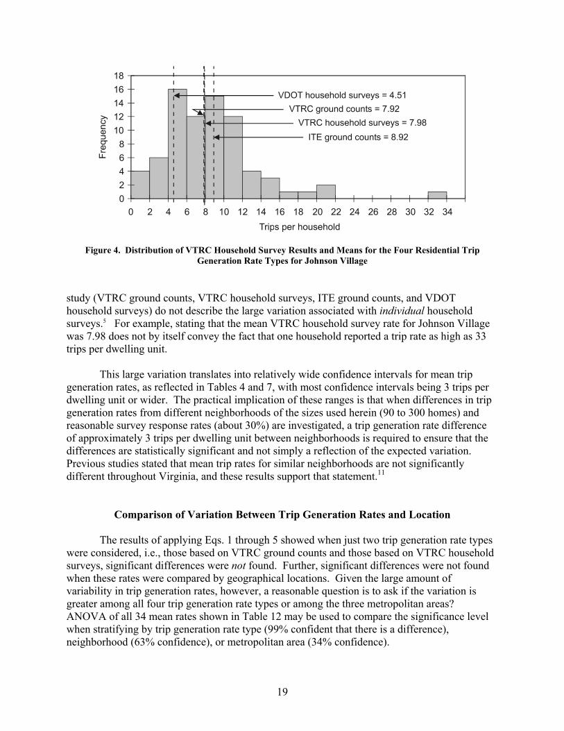
The trip generation rates showed substantial random variation that is not readily explained by geography. Figure 4 illustrates this variation for an individual neighborhood, where it is apparent that the mean trip generation rates for the four types computed during this
19
Figure 4. Distribution of VTRC Household Survey Results and Means for the Four Residential Trip Generation Rate Types for Johnson Village
study (VTRC ground counts, VTRC household surveys, ITE ground counts, and VDOT household surveys) do not describe the large variation associated with individual household surveys.5 For example, stating that the mean VTRC household survey rate for Johnson Village was 7.98 does not by itself convey the fact that one household reported a trip rate as high as 33 trips per dwelling unit.
This large variation translates into relatively wide confidence intervals for mean trip generation rates, as reflected in Tables 4 and 7, with most confidence intervals being 3 trips per dwelling unit or wider. The practical implication of these ranges is that when differences in trip generation rates from different neighborhoods of the sizes used herein (90 to 300 homes) and reasonable survey response rates (about 30%) are investigated, a trip generation rate difference of approximately 3 trips per dwelling unit between neighborhoods is required to ensure that the differences are statistically significant and not simply a reflection of the expected variation. Previous studies stated that mean trip rates for similar neighborhoods are not significantly different throughout Virginia, and these results support that statement.11
Comparison of Variation Between Trip Generation Rates and Location
The results of applying Eqs. 1 through 5 showed when just two trip generation rate types were considered, i.e., those based on VTRC ground counts and those based on VTRC household surveys, significant differences were not found. Further, significant differences were not found when these rates were compared by geographical locations. Given the large amount of variability in trip generation rates, however, a reasonable question is to ask if the variation is greater among all four trip generation rate types or among the three metropolitan areas? ANOVA of all 34 mean rates shown in Table 12 may be used to compare the significance level when stratifying by trip generation rate type (99% confident that there is a difference), neighborhood (63% confidence), or metropolitan area (34% confidence).
20
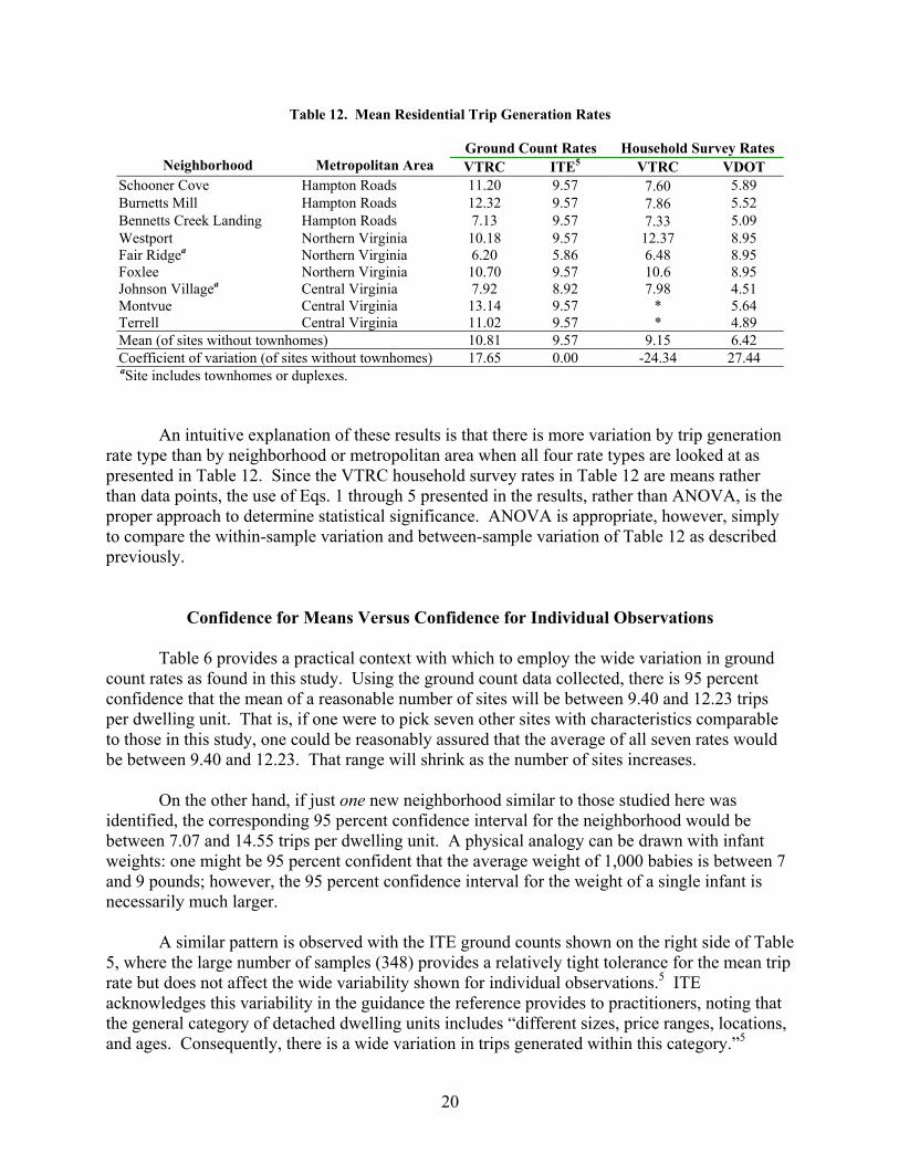
Table 12. Mean Residential Trip Generation Rates
Ground Count Rates Household Survey Rates Neighborhood
Metropolitan Area VTRC ITE5 VTRC VDOT
Schooner Cove Hampton Roads 11.20 9.57 7.60 5.89 Burnetts Mill Hampton Roads 12.32 9.57 7.86 5.52 Bennetts Creek Landing Hampton Roads 7.13 9.57 7.33 5.09 Westport Northern Virginia 10.18 9.57 12.37 8.95 Fair Ridgea Northern Virginia 6.20 5.86 6.48 8.95 Foxlee Northern Virginia 10.70 9.57 10.6 8.95 Johnson Villagea Central Virginia 7.92 8.92 7.98 4.51 Montvue Central Virginia 13.14 9.57 * 5.64 Terrell Central Virginia 11.02 9.57 * 4.89 Mean (of sites without townhomes) 10.81 9.57 9.15 6.42 Coefficient of variation (of sites without townhomes) 17.65 0.00 -24.34 27.44
aSite includes townhomes or duplexes.
An intuitive explanation of these results is that there is more variation by trip generation
rate type than by neighborhood or metropolitan area when all four rate types are looked at as presented in Table 12. Since the VTRC household survey rates in Table 12 are means rather than data points, the use of Eqs. 1 through 5 presented in the results, rather than ANOVA, is the proper approach to determine statistical significance. ANOVA is appropriate, however, simply to compare the within-sample variation and between-sample variation of Table 12 as described previously.
Confidence for Means Versus Confidence for Individual Observations
Table 6 provides a practical context with which to employ the wide variation in ground count rates as found in this study. Using the ground count data collected, there is 95 percent confidence that the mean of a reasonable number of sites will be between 9.40 and 12.23 trips per dwelling unit. That is, if one were to pick seven other sites with characteristics comparable to those in this study, one could be reasonably assured that the average of all seven rates would be between 9.40 and 12.23. That range will shrink as the number of sites increases.
On the other hand, if just one new neighborhood similar to those studied here was identified, the corresponding 95 percent confidence interval for the neighborhood would be between 7.07 and 14.55 trips per dwelling unit. A physical analogy can be drawn with infant weights: one might be 95 percent confident that the average weight of 1,000 babies is between 7 and 9 pounds; however, the 95 percent confidence interval for the weight of a single infant is necessarily much larger.
A similar pattern is observed with the ITE ground counts shown on the right side of Table 5, where the large number of samples (348) provides a relatively tight tolerance for the mean trip rate but does not affect the wide variability shown for individual observations.5 ITE acknowledges this variability in the guidance the reference provides to practitioners, noting that the general category of detached dwelling units includes “different sizes, price ranges, locations, and ages. Consequently, there is a wide variation in trips generated within this category.”5

21
Choosing the Appropriate Confidence Interval
The next question is: “Which confidence interval, i.e., that for means or that for individual observations, is correct?” The answer depends on how the trip generation rates are applied. To the extent that planners want to use a trip generation rate from this effort in lieu of a field study, they would be advised to use the 95 percent confidence interval associated with an individual observation. Thus if the neighborhood of interest is comparable to the VTRC neighborhoods, approximately 95 percent of the time, the trip generation rate for the individual neighborhood will be between 7.07 and 14.55 trips. For many applications, therefore, such a wide confidence interval will not be suitable; thus, field studies would be recommended.
On the other hand, there may be applications that will in fact use data from multiple neighborhoods, such as the subarea study. As the number of neighborhoods encompassed within the subarea study increases, the confidence interval associated with the mean rates becomes appropriate. Informally, this concept may be explained as the law of large numbers: a mean trip generation rate close to 10.81 is more likely to be obtained if the mean is based on 10 rather than 2 neighborhoods. Using the data from Table 6, if a trip generation rate was needed for a subarea of seven residential neighborhoods, the 95 percent confidence interval would be 9.40 to 12.23 trips per dwelling unit.
Limitations and Assumptions in Establishment of Confidence Intervals
Four assumptions are implicit in the application of the confidence intervals in Table 5 to future efforts.
1. The characteristics of neighborhoods in future efforts are comparable to those in this study. The variation in the individual observations (e.g., the VTRC ground counts from each of the seven neighborhoods) is not explained by a characteristic unique to this study. For example, neighborhoods with larger homes, more expensive homes, or homes located further from the central business district will tend to have higher trip generation rates than average.5 Thus, if a set of revitalized infill neighborhoods being constructed close to the central business district is being studied, then presumably a lower trip generation rate than has been reported here would be expected.
2. Data are normally distributed. Although the shape of the VTRC ground count data
appears to be normal, this determination is difficult to make with only seven observations. An alternative, however, is to compare the theoretical and actual confidence bounds. Table 13 shows the 95 percent confidence bounds as computed from Eq. 2 and the 100 percent confidence bounds actually found, e.g., the full range of data points. Interestingly, for VTRC, the 100 percent actual confidence bounds are narrower than the 95 percent theoretical bounds, suggesting that these data may follow a distribution similar to that of the normal distribution but with a much tighter band.

22
Table 13. 95 Percent Theoretical Confidence Interval and 100 Percent Actual Confidence Interval
Interval VTRC Ground
Counts ITE Ground
Counts5 Sample Size (number of neighborhoods) 7 348 Theoretical Lower 95% Bound for Individual Observations 7.07 2.34 Theoretical Upper 95% Bound for Individual Observations 14.55 16.80 Actual 100% Lower Bound for Individual Observations 7.13 4.31 Actual 100% Upper Bound for Individual Observations 13.14 21.85
3. All sources of variation are adequately reflected in Table 6. If a ground count is performed on two days, there will be some variation between the two numbers. For example, Table 3 shows the Westport neighborhood as having a ground count trip rate of 10.18; this neighborhood was surveyed by VTRC twice, and the first time it had a ground count rate of 9.45. The 9.45 figure was not used because of problems with other aspects of that day’s data collection, which necessitated a restudy of the neighborhood.
4. The Z statistic of 1.96 is appropriate for these sample sizes. When establishing
confidence bounds, statisticians usually use the T statistic rather than the Z statistic for relatively small sample sizes. Using the Z statistic rather than the T statistic in Eq. 5 for establishing the confidence bounds shown in Table 13 means that the theoretical bounds reflect the 90 percent confidence interval rather than the 95 percent confidence interval. Because this difference is relatively small and to encourage replication of confidence intervals for other data sets beyond those presented here, this study used the Z statistic consistently for the computation of confidence intervals.
Role of Proportion of Trips Made by Residents
The proportion of trips made by residents, reflected in Tables 9 and 10, was investigated since it was thought that differences in these proportions might explain differences between household survey trip generation rates and ground count trip generation rates. No statistically significant relationship, however, was found.
The proportion of trips made by residents did yield two insights that were not previously apparent and possibly corroborated a third observation from the literature.
• Even with the inclusion of uncertainty about data collection and statistical variation, Table 11 shows that the proportions of trips made by residents were significantly different among the two data collection methods, as the intervals did not overlap except for the interval for Bennetts Creek Landing. Thus the explanation for the differences is some factor other than data collection error for ground counts or expected variation for neighborhood surveys.
23
• The width of the confidence intervals suggests that unlike data collection errors, statistical variation is a longer term phenomenon that cannot be eliminated. Improvements to data collection reduced the width of the confidence interval reflected by the left half of Table 11 such that the last neighborhood the investigators studied, Westport B, had a very tight tolerance. On the other hand, the size of the confidence intervals reflected by the right half of the table, although generally between 7 and 10 percentage points, grew as large as 20 percentage points for two of the neighborhoods.
• The literature suggests that residents underreport trips, especially trips that are not
made with regularity (e.g., retail trips are more likely to be underreported than work trips).12,13 Extending that reasoning to the VTRC household survey, which asked residents to report not just their own trips but also trips made by nonresidents who visited them, it is possible that the VTRC survey results indicated a lower proportion of nonresident trips than what occurred. That behavior is a plausible, but not proven, explanation for why the proportion of trips made by residents is higher when surveys rather than ground counts are the basis.
Can Underreporting Explain Differences Between Ground Count and Household Survey Rates?
Although Table 3 indicated that the mean VTRC ground count rate of 10.81 was higher
than the mean VTRC household survey rate of 9.16 for single-family detached homes, the difference between these mean rates was not statistically significant (79% confidence). Based on these data alone and a strict adherence to the 95 percent confidence threshold, therefore, it cannot be concluded that underreporting, if it is occurring, is causing a significant difference in these rates.
The suggestion of underreporting in the literature, however, coupled with the observations of this study, suggests that underreporting of trips is a strong possibility. A larger number of additional studies may continue to show that the mean ground count rate is higher than the mean household survey rate. If statistical tests confirm that the differences are significant (e.g., at 95% confidence or greater), underreporting or some other phenomenon necessitates that these rates be treated differently. In that instance, when a model calls for a ground count rate but the available datum is a household survey rate (or vice-versa), an adjustment to make the rates compatible would become appropriate. Appendix C explores some additional techniques that may be used to focus strictly on underreporting.
CONCLUSIONS 1. Large and random variation exists among residential trip generation rates for residential
neighborhoods. For the seven neighborhoods with only single-family detached dwelling units in this study, an analyst can be 95 percent confident that the mean rate according to

24
ground counts is between 9.4 and 12.2 trips per dwelling unit. Yet the corresponding 95 percent confidence interval for any single neighborhood is between 7.1 and 14.6 trips per dwelling unit. These observations are consistent with the large variation reported by ITE.5 To the extent that subarea studies contain multiple neighborhoods as opposed to just one neighborhood, the confidence intervals for mean rates as opposed to a single value are appropriate.
2. Large variations imply that large numerical differences do not necessarily reflect statistical
significance. Specifically, tests of significance at the 95 percent confidence threshold support four conclusions:
• Generally, there was no significant difference between the mean residential trip
generation rate based on VTRC ground counts and the mean rate based on VTRC household surveys. An exception to this rule was found for two of the seven neighborhoods studied. Appendix C illustrates how additional personal data could, however, be used in future efforts to determine better whether underreporting does occur.
• Generally, there was no significant difference among mean residential trip generation
rates from different locations. When rates were aggregated by metropolitan area, no significant differences in the means were found, regardless of how the trip generation rate was defined. When examined by individual neighborhoods, significant differences were found in the trip generation rate based on VTRC household surveys; however, all of these occurred in neighborhoods with fewer than 30 survey responses.
• VTRC ground count rates were statistically similar to those of national ITE rates, which
are also based on ground counts.5 In short, VTRC field data were similar to national data when ground counts were performed.
• Rates based on VTRC household surveys, however, were different from rates based on
long-range VDOT planning models. Findings from this study suggest that a contributing factor to this discrepancy was the conversion from person trips to vehicle trips that was required for the VDOT long-range model at six of the nine sites. In short, VTRC field data were different from VDOT regional data when surveys were conducted where VTRC had surveyed vehicle trips directly and VDOT had surveyed person trips and then converted those responses to vehicle trips.
3. Given that variation is present in the mean residential trip generation rates from all four
sources, more of the variation can be attributed to differences in how rates are defined as opposed to differences in location. The implication is that it is more important to define a residential trip generation rate consistently than to collect rates for different regions. “Defining” the rate means specifying (1) whether the basis is a ground count or a household survey, (2) whether the rate is an average value for the region/nation or is an individual value collected for a particular neighborhood, and (3) whether the rate measures vehicle trips directly or instead measures person trips and then requires some type of automobile occupancy data to make the conversion to vehicle trips.

25
4. The proportion of trips made by neighborhood residents averaged 67 percent when ground counts were the basis and 77 percent when household surveys were the basis. Statistical variation and uncertainty about data collection do not account for this difference. A plausible explanation for this difference is that residents underreported nonresident trips, since these trips tend to be irregular and the literature indicates that irregular trips are more likely to be underreported.13 Underreporting was indicated by this study at the confidence level of 79 percent; thus a preponderance of evidence suggests underreporting is likely, but this evidence is not sufficiently strong to prove underreporting at the conventional confidence threshold of 95 percent.
5. Use of the revised data collection methodology described in Appendix A helped reduce data
collection errors. Several data collection approaches were used throughout this study, and the approach that minimizes the uncertainty documented in Appendix A is presented in this report.
RECOMMENDATIONS
1. When a ground count rate for an individual neighborhood is needed, VDOT should ideally conduct a field study of the neighborhood, given the high variability among individual neighborhoods reported in this study and by ITE.5 The results of this study indicate that for one neighborhood comprised of single-family detached dwelling units, an analyst can be 95 percent confident that the trip generation rate will be between 7.1 and 14.6 trips per dwelling unit.
2. When a mean ground count rate for a subarea consisting of a group of neighborhoods is
needed, VDOT should either conduct a field study or use the 95 percent confidence interval for mean observations, similar to what is presented in Table 6. For example, this study indicates that an analyst can be 95 percent confident that for seven neighborhoods comprised solely of single-family detached homes, the mean trip generation rate is between 9.4 and 12.2 trips per dwelling unit. ITE values overlap with the lower portion of this range.5
3. Before performing a field study, analysts should conduct a sensitivity analysis with the two
trip generation rates that signify the lower and upper bound of the appropriate 95 percent confidence interval. There may be situations where despite a wide difference between the upper and lower trip generation rate, the result of the entire modeling process is not significantly affected regardless of which trip generation rate is chosen. In those situations, trip generation data collection is not likely to be helpful for the problem being studied.
4. When conducting field studies, planners should use the data collection methodology
described in Appendix A. The method shown in Appendix A reflects insights from VDOT staff and VTRC staff who performed data collection in the nine neighborhoods studied.
5. Through VTRC’s Transportation Planning Research Advisory Committee, VDOT should
archive ground count trip generation rates and household survey trip generation rates that are obtained through field studies. One potential benefit of archiving such studies would be
26
to confirm or refute the possibility that underreporting in survey responses leads to a residential trip generation rate based on household surveys being lower than a rate based on ground counts.
ACKNOWLEDGMENTS
The investigators are grateful to the many persons who provided assistance with this study: J. Wade of the Albemarle County Planning Department; T. Vest of the City of Charlottesville Planning Department; F. Khaja of the Fairfax County Department of Planning; C. Draper of the Loudoun County Planning Department; E. Azimi, U. Bellinger, C. Bilinski, D. Claud, E. Stringfield, and W. Mann of the Virginia Department of Transportation; K. Tew, R. Pierce, and R. Moore of the Hampton Roads Planning District Commission; and J. Fang, O. Hijaz, E. Johnson, J. Labrie, S. Martin, K. Mossman, K. Peacock, K. Spence, D. Thomas, J. Van Doren, and L. Woodson of the Virginia Transportation Research Council.
REFERENCES
1. Institute of Transportation Engineers. Transportation Planning Handbook, J. Edwards (ed.).
Prentice-Hall, Inc., Englewood Cliffs, N.J., 1992. 2. Federal Highway Administration. NHI Course No. 152054: Introduction to Urban Travel
Demand Forecasting. Publication No. FHWA-NHI-02-040. Washington, D.C., March 2002, pp. 5-25.
3. Horowitz, A.J. Subarea Focusing with Combined Models of Spatial Interaction and
Equilibrium Assignment. Transportation Research Record 1285. Transportation Research Board, Washington, D.C., 1990, pp. 1-8.
4. Winslow, K.B., Bladikas, B.K., Hausman, K.J., and Spasovic, L.N. Introduction of
Information Feedback Loop to Enhance Urban Transportation Modeling System. Transportation Research Record 1493. Transportation Research Board, Washington, D.C., 1995, pp. 81-90.
5. Institute of Transportation Engineers. Trip Generation, 6th ed. Washington, D.C., 1997. 6. Dawoud, M. Personal Communication, June 2002 and April 2003. 7. Mann, W.E. Personal Communication, January 2003 and April 2003. 8. Pedersen, N.J., and Samdahl, D.R. National Cooperative Highway Research Program
Report 255: Highway Traffic Data for Urbanized Area Project Planning and Design. Transportation Research Board, Washington, D.C., 1982.

27
9. Cervero, C.C. Impacts of Zonal Reconfigurations on Travel Demand Forecasts.
Transportation Research Record 1305. Transportation Research Board, Washington, D.C., 1991, pp. 72-80.
10. Montgomery, D.C. Introduction to Statistical Quality Control, 4th ed. John Wiley & Sons,
Inc., New York, 2001. 11. Arnold, E.D. Special Land Use Trip Generation in Virginia. VTRC 81-R35. Virginia
Transportation Research Council, Charlottesville, 1981. 12. Reid, F.A. Critique of ITE Trip Generation Rates and An Alternative Basis for Estimating
New Area Traffic. Transportation Research Record 874. Transportation Research Board, Washington, D.C., 1982, pp. 1-5.
13. Kumar, A., and Levinson, D. Specifying, Estimating, and Validating a New Trip Generation
Model: Case Study in Montgomery County, Maryland. Transportation Research Record 1413. Transportation Research Board, Washington, D.C., 1993, pp. 107-113.

28
29
APPENDIX A
DATA COLLECTION METHODOLOGY
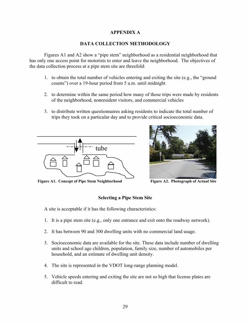
Figures A1 and A2 show a “pipe stem” neighborhood as a residential neighborhood that has only one access point for motorists to enter and leave the neighborhood. The objectives of the data collection process at a pipe stem site are threefold:
1. to obtain the total number of vehicles entering and exiting the site (e.g., the “ground counts”) over a 19-hour period from 5 a.m. until midnight
2. to determine within the same period how many of those trips were made by residents
of the neighborhood, nonresident visitors, and commercial vehicles
3. to distribute written questionnaires asking residents to indicate the total number of trips they took on a particular day and to provide critical socioeconomic data.
tube
Figure A1. Concept of Pipe Stem Neighborhood Figure A2. Photograph of Actual Site
Selecting a Pipe Stem Site
A site is acceptable if it has the following characteristics:
1. It is a pipe stem site (e.g., only one entrance and exit onto the roadway network).
2. It has between 90 and 300 dwelling units with no commercial land usage.
3. Socioeconomic data are available for the site. These data include number of dwelling units and school age children, population, family size, number of automobiles per household, and an estimate of dwelling unit density.
4. The site is represented in the VDOT long-range planning model.
5. Vehicle speeds entering and exiting the site are not so high that license plates are
difficult to read.

30
Tasks That Should Be Accomplished 1 Week Prior to Collecting Field Data 1. Email or fax a letter to local law enforcement and local planners associated with the city,
county, PDC, and/or MPO. A sample letter is shown as Figure A3. 2. Distribute letters to the residents of the community. Letters should be placed inside a
newspaper box or under the front door mat but not inside a mailbox. A sample letter is shown as Figure A4.
3. Distribute questionnaires to residents the same day on which the letters were delivered. The
written questionnaire is shown in Figure A5 and was delivered with postage already attached.
• One VDOT planner suggested that a response rate can be increased if one affixes stamps rather than using prepaid “No postage necessary” envelopes.
• The household survey should be completed by residents for the same day as the ground
counts are collected. This ensures that if data are collected on an abnormal travel day for the neighborhood, it is reflected in both the ground counts and the survey data.
Tasks That Should Be Performed Immediately Before, During, and After Data Collection
The steps shown presume the tube counters or other measurement devices were placed on
a Tuesday, that counts were taken on a Wednesday, and that tube counters were removed on a Thursday.
Tuesday: Day Before Ground Counts Collected 1. Have data collectors meet to review data collection and safety procedures. It is critical that
two data collectors be present at all times and that one of the two be an experienced agency employee. Each data collector should have a VDOT identification card, a driver’s license, or other form of personal identification and copies of the letters shown in Figures A3 and A4.
2. Ensure data collectors are ready to respond to residents who may ask them questions. In
particular, data collectors should note that the use of license plates is solely to identify trips entering and exiting made by the same vehicle and not to record personal information.
3. Print copies of the data collection forms shown in Figure A6. 4. Have two data collectors place a tube counter (or other measurement device) at the pipe stem
to obtain ground counts, stratified by half-hour intervals. Generally, tube counters should be left in place for approximately 48 hours.

31
Wednesday: Day Ground Counts Collected
A site requires four to six people, with two collectors per shift. An example of a three-shift schedule is given here. The shifts overlapped so that each group had about a half-hour transition on either side of their shift.
Shift Time 1 4:30 a.m. to 11:30 a.m. 2 11:00 a.m. to 6:00 p.m. 3 5:30 p.m. to midnight
The main task of the data collectors is to record the last five digits of the license plates of vehicles entering and leaving the neighborhood and a short description. The description should include the following at a minimum:
• the state of the vehicle if a state other than Virginia • the color and type of vehicle OR
• a description of the business if the vehicle is a commercial vehicle.
If time permits, the data collectors should also provide
• more detailed vehicle descriptions • a notation in the margin when the collectors recognize the same vehicle entering and
exiting the site
• arrows between the columns of Figure A6 when the same vehicle enters and exits during a 15-minute interval.
Thursday: Day After Ground Counts Collected
Data collectors should remove tube counters or other measurement device and download the data contained therein.

32
Sgt. Ernest Allen Albemarle County Police Department Ron Higgins Charlottesville Planning Department Sgt. Ronnie Roberts Charlottesville Police Department Juan Diego Wade Albemarle County Planning Office Bill Wanner Thomas Jefferson Planning District Commission Dear Sgt. Allen, Mr. Higgins, and Sgt. Roberts, Mr. Wade, and Mr. Wanner, I wanted to let you know that we (the Virginia Department of Transportation) will be conducting a traffic study of trip generation rates in Charlottesville and Albemarle County in three specific neighborhoods: Terrell (Thursday, October 18) Johnson Village (Thursday, October 25) Montvue (Tuesday October 30) VDOT would like to better quantify the number of trips generated by residential neighborhoods that are comprised solely of single-family detached dwelling units or townhomes. These neighborhoods are found in different areas of the state and are increasingly common in exurban areas (e.g. one of the drivers for our interest are recent residential developments in Loudoun County). As an initial part of this study, we (Jared Ulmer, Les Hoel, Lewis Woodson, and myself) will be collecting trip generation data for a single day at a few Charlottesville neighborhoods beginning in October. At each site, we will record the number of vehicle trips entering and exiting, as well as the last five digits of the license plate. (The partial license plate information enables us to simply estimate the number of trips that originate and terminate in the neighborhood as opposed to those that originate elsewhere, but will not be used by us to identify the owners’ vehicles.) We will also lay down pneumatic tubes to assist us with obtaining accurate vehicle counts. We are distributing flyers similar to this letter to residents in these neighborhoods. If you can recommend any contacts from neighborhood associations for these areas, so that we can ensure they are aware of our study. If you would like additional information, please do not hesitate to contact me. John Miller, Virginia Transportation Research Council, 434-293-1999 John Miller Virginia Transportation Research Council 530 Edgemont Road Charlottesville, Virginia 22903 (434) 293-1999 (voice) (434) 293-1990 (fax)
Figure A3. Sample Letter Sent to Local Authorities
33
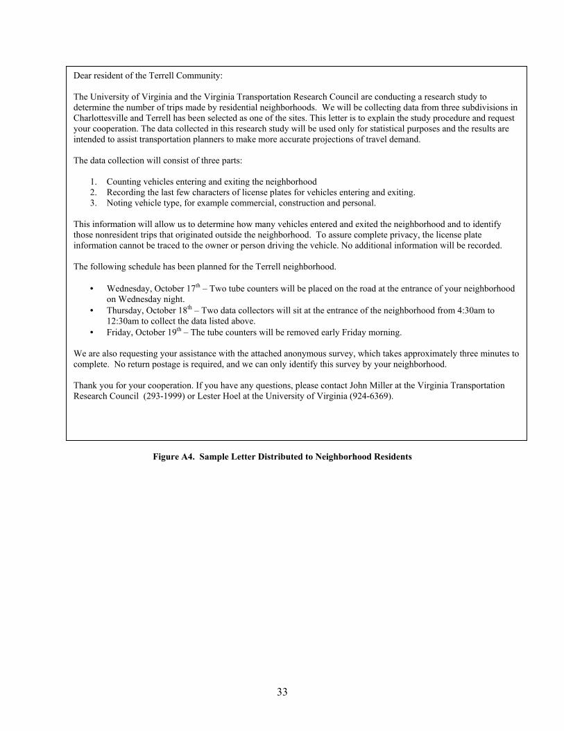
Figure A4. Sample Letter Distributed to Neighborhood Residents
Dear resident of the Terrell Community: The University of Virginia and the Virginia Transportation Research Council are conducting a research study to determine the number of trips made by residential neighborhoods. We will be collecting data from three subdivisions in Charlottesville and Terrell has been selected as one of the sites. This letter is to explain the study procedure and request your cooperation. The data collected in this research study will be used only for statistical purposes and the results are intended to assist transportation planners to make more accurate projections of travel demand. The data collection will consist of three parts:
1. Counting vehicles entering and exiting the neighborhood 2. Recording the last few characters of license plates for vehicles entering and exiting. 3. Noting vehicle type, for example commercial, construction and personal.
This information will allow us to determine how many vehicles entered and exited the neighborhood and to identify those nonresident trips that originated outside the neighborhood. To assure complete privacy, the license plate information cannot be traced to the owner or person driving the vehicle. No additional information will be recorded. The following schedule has been planned for the Terrell neighborhood.
• Wednesday, October 17th – Two tube counters will be placed on the road at the entrance of your neighborhood on Wednesday night.
• Thursday, October 18th – Two data collectors will sit at the entrance of the neighborhood from 4:30am to 12:30am to collect the data listed above.
• Friday, October 19th – The tube counters will be removed early Friday morning. We are also requesting your assistance with the attached anonymous survey, which takes approximately three minutes to complete. No return postage is required, and we can only identify this survey by your neighborhood. Thank you for your cooperation. If you have any questions, please contact John Miller at the Virginia Transportation Research Council (293-1999) or Lester Hoel at the University of Virginia (924-6369).

34
Dear resident of Terrell: The University of Virginia and the Virginia Transportation Research Council are conducting a research study to determine the number of trips made from residential neighborhoods. The results are intended to assist transportation planners to make more accurate projections of travel demand in Virginia. We are requesting your assistance with the attached anonymous survey, which takes approximately three minutes to complete. The data collected in this research study will be used for general statistical purposes only and we cannot identify any individual by the survey. Please fold & tape the survey and send by return mail. No postage is required. Thank you for your cooperation. If you have any questions, please contact John Miller at the Virginia Transportation Research Council (293-1999) or Lester Hoel at the University of Virginia (924-6369). _____________________________________________________________________________________________ 1. Last Tuesday, how many total round trips were made by all members living in your household who drove a motor vehicle? (*If you cannot remember the last Tuesday you can use the upcoming Tuesday.) A round trip is a trip from your home that leaves Terrell for any purpose and any length of time and then returns to your home within the same day. a. Leaving between 5:00 am and midnight? _______ b. Leaving between midnight and 5:00 am? _______ 2. Last Tuesday, how many total round trips were made by all members of your household by each of the following modes? (*If you cannot remember the last Tuesday you can use the upcoming Tuesday.) A round trip is a trip from your home that leaves Terrell for any purpose and any length of time and then returns to your home within the same day. a. Walking (do not include walking just for exercise) _______ b. Biking (do not include biking just for exercise) _______ c. Public transit _______ d. Passenger in a taxi _______ e. Passenger in a carpool or any private vehicle _______ 3. Please indicate the number of: a. Members living in your household _______ b. Licensed drivers in your household _______ c. Household members who drive to work or school _______ d. Household members who work or attend school but do not drive _______ e. Vehicles available to your household _______ 4. Last Tuesday, how many commercial or business vehicles visited your household? *_______
*Exclude newspaper, U.S. mail, UPS, FedEx, and trash services. 5. Last Tuesday, how many private vehicles visited your household? **_______ **Include social visits, errands, carpools picking up/dropping off a household member, etc.
Figure A5. Revised Household Survey
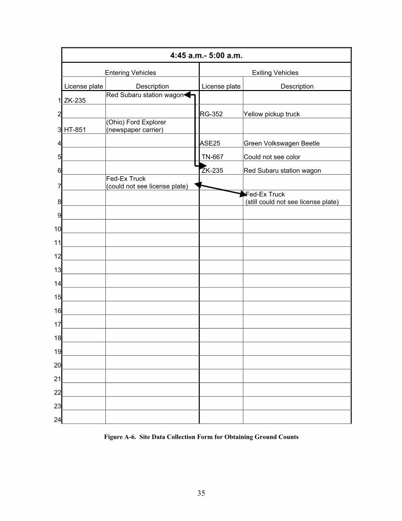
35
4:45 a.m.- 5:00 a.m.
Entering Vehicles Exiting Vehicles
License plate Description License plate Description
1 ZK-235 Red Subaru station wagon
2 RG-352 Yellow pickup truck
3 HT-851 (Ohio) Ford Explorer (newspaper carrier)
4 ASE25 Green Volkswagen Beetle
5 TN-667 Could not see color
6
ZK-235 Red Subaru station wagon
7 Fed-Ex Truck (could not see license plate)
8 Fed-Ex Truck (still could not see license plate)
9
10
11
12
13
14
15
16
17
18
19
20
21
22
23
24
Figure A-6. Site Data Collection Form for Obtaining Ground Counts

36

37
APPENDIX B
HOW THE FOUR TRIP GENERATION RATES WERE COMPUTED
Data from the Johnson Village neighborhood are presented here to illustrate how the four trip generation rates (based on VTRC ground counts, VTRC household surveys, ITE ground counts, and VDOT long-range planning models) were computed. The first step also shows how confidence bounds were created that reflect data collection uncertainty associated with the proportion of trips generated by nonresidents.
Step 1. Calculate the VTRC ground count trip rates.
After the information was recorded at each site during the ground counts, the data were entered into a spreadsheet. A program was written and used to assist in matching license plates and classifying each vehicle as resident, nonresident, or commercial. With some exceptions, a pair of license plates was considered as a resident match if a match occurred with the exiting movement occurring earlier than the entering movement. The reverse applied for a nonresident match. Commercial vehicles were indicated as such at the site and accordingly entered into the spreadsheet. Some license plates could not be matched and were classified as unknown.
Due to imperfect data collection, the spreadsheet program was unable to pinpoint an exact number of vehicles in the resident and nonresident categories. Instead, the program was used to develop a range of values for these categories. In the case of uncertainty for a given match, the program was run twice to favor each possibility separately. This resulted in a minimum and maximum number of resident and nonresident vehicles.
To simplify the data analysis, an “estimated mean” was found for resident and nonresident vehicle trips. To find this estimated mean, the trips were first divided into resident matches, nonresident matches, and undetermined matches. Rather than splitting the undetermined matches evenly between the resident and nonresident categories, the undetermined matches were weighted so that they were distributed in relation to the matches we made with certainty. For example, before distributing the undetermined matches, the trips that have been matched with certainty and the percentage of resident and nonresident trips for Johnson Village are listed along with the undetermined matches in Table B1. Table B2 shows the estimate of undetermined trips that should be added to resident and nonresident categories.
Table B1. Number of Resident, Nonresident, and Undetermined Trips
Category Trips % Total Resident 1039 78.5 Nonresident 284 21.5 Undetermined 76
The undetermined matches are multiplied by the percentage of each matched category to weigh the undetermined matches in relation to the matches already made.

38
Table B2. Estimate Undetermined Trips That Should Be Added to Resident and Nonresident Categories
Category Trips % Total Add to resident 60 78.5 Add to nonresident 16 21.5 Total 76 100
Finally, as shown in Table B3, these newly calculated trips are added to the previous certain matches to compute the total estimated mean for these two trip categories, maintaining the original proportion of resident trips to nonresident trips.
Table B3. Calculate Means of Estimated Resident and Nonresident Trips
Category Trips % Total Resident 1,099 78.5 Nonresident 300 21.5
Note that commercial vehicles were not subject to this uncertainty (as license plates were often not even required to identify and match them), so this vehicle classification was calculated as a single value.
The preceding calculation was used on license plates that were correctly matched to other license plates but with uncertainty as to whether the match was a resident or nonresident match. There is also a group of license plates that could not be matched to other plates. This number was usually close to 10 percent of the total number of license plates unless major data collection problems occurred at a site. These unmatched vehicles were distributed in a manner similar to the one described to the resident and nonresident categories. Finally, for each vehicle category and for all vehicles, the number of trips was divided by the number of households to determine the VTRC ground count rates for each development. Table B4 shows the final VTRC ground count rates for Johnson Village.
Table B4. Summary of VTRC Ground Count Trip Rates for Johnson Village
Resident Favored Estimated Mean Nonresident Favored Category trips trips/du % total trips trips/du % total trips trips/du % total Resident 1244 5.60 70.7 1227 5.52 69.7 1159 5.22 65.9 Nonresident 317 1.43 18.0 334 1.50 19.0 402 1.81 22.8 Commercial 198 0.89 11.3 Total 1759 7.92 100.0

39
Step 2. Calculate the VTRC household survey trip rates.
Household surveys were mailed back to VTRC, and the data were entered into a spreadsheet. From the survey responses, the number of resident, nonresident, commercial, and total trips for each household could be determined. Table B5 shows the Johnson Village results.
Table B5. Summary of VTRC Household Survey Trip Rates for Johnson Village
Category
Trips
Trips/ Dwelling Unit
% Total
Resident 1,356 6.03 75.5 Nonresident 281 1.25 15.6 Commercial 160 0.71 8.9 Total 1,796 7.98 100.0
Step 3. Calculate the ITE ground count trip rates.
Computation of the ITE ground count rates allowed for the VTRC ground count trip rates to be compared to the standard trip rates published in the nationally based ITE Trip Generation.5 The values in Trip Generation are listed as vehicle trips/dwelling unit for various types of dwelling units. These values were then multiplied by the percentage of each dwelling category in the neighborhoods. For example, for Johnson Village, the ITE trip generation rate was an average of 8.92 trips per dwelling unit.
Because Johnson Village had duplexes that from visual inspection of the neighborhood
were thought to contribute to trip generation rates comparable to those for single-family detached dwelling units, the higher ITE rate for “apartments” shown in Table B6 was used rather than the lower ITE rate for “townhouses.” Because the Fair Ridge neighborhood had townhomes, however, the lower ITE rate associated with “townhouses” was used. The remaining seven neighborhoods had only single-family detached dwelling units and hence required only the ITE rate for “single-family residential” shown in Table B6.
Table B6. Calculation of ITE Ground Count Trip Rate for Johnson Village
ITE5 VTRC Dwelling Unit Category
Trips/ Dwelling Unit
No. of Dwelling Units
% Total
Trips/ Dwelling Unit
Single-family residential 9.57 175 77.8 7.45 Apartments 6.63 50 22.2 1.47 Townhouses 5.86 Mobile homes 4.81 Planned unit developments 7.50 Total 225 100.0 8.92
40
Step 4. Calculate the VDOT household survey trip rates.
This calculation allowed for the VTRC household survey trip rates to be compared to the trip rates developed in VDOT’s long-range planning model based on household survey data. For the Charlottesville/Albemarle region, the VDOT model data are derived from the trip production cross-classification table in the Route 250 Corridor Study, Charlottesville, Virginia, 1997 Traffic Model Methodology Report (prepared for VDOT by Michael Baker, Jr., Inc., April 1999). Route 250 Corridor Study, Charlottesville, Virginia, 1997 Traffic Model Methodology Report.
Person trips were not converted to vehicle trips, as observations showed that non-vehicle trips were negligible. (Table 6.2 of Appendix B in the Route 250 Corridor Study gives automobile occupancy rates of 1.17, 1.70, and 1.50, respectively, for home-based work, home-based other, and non-home-based trip rates. However, since those are based on 1987 data, it appeared more appropriate to use observations at the site.)
The rationale for performing the detailed computations shown in Tables B7 through B10 is to replicate the methodology of the long-range regional model using current data. Updated socioeconomic data such as automobile ownership and household size enable the study to focus on the reasoning underlying the regional model.
Table B8 provides the data given by neighborhood residents through the household
surveys regarding household size and vehicle ownership. The home-based work and home-based other rates from Table B7 were multiplied by the
corresponding cells for each cross-classification category in Table B8 to determine the total number of trips made by all residents in each category. Non-home-based trips were not used because these did not reflect traffic that would be entering and exiting the neighborhood and thus would not be recorded during the ground counts.
To calculate the trips made by nonresidents and commercial vehicles, the portions of the
trip attraction equations dependent on households were used. For home-based other attractions in Johnson Village, a rate of 0.385 trip/household was used. For non-home-based attractions, the published rate of 0.345 trip/household was multiplied by 2 to account for the non-home-based productions that must be associated with these trips. The reason for doubling the non-home-based attractions is formally explained in the literature as follows: “We discard the NHB productions generated in the ‘home’ TAZ (transportation analysis zone) and substitute them with the NHB attraction for that TAZ, assuming that people attracted to that TAZ will be produced out of that TAZ.” Thus although Johnson Village data indicate 0.345 NHB attraction per household, this figure means that each household attracts 0.345 trip as the destination end of the NHB trip and then each household generates 0.345 trip as the origin end of another NHB trip. Computationally, therefore, there is 0.690 NHB trip per household.2
The trip production values in Table B9 were added to the trip attractions to determine the total number of trips made by the survey respondents. By dividing the total trips by the number of survey respondents, the VDOT household survey trip rate is computed.

41
Table B7. VDOT Cross-Classification Table for Charlottesville/Albemarle Region
Household (Family) Size Autos per Household
1 2 3 4+ Trip Purpose
0.39 0.50 0.65 0.75 Home-based work 0.76 1.38 2.15 3.20 Home-based other 0 1.39 1.39 1.40 1.40 Non-home-based 0.83 0.90 1.40 1.43 Home-based work 1.86 2.80 3.80 6.17 Home-based other 1 1.72 2.01 2.40 2.49 Non-home-based 0.88 1.39 1.73 1.89 Home-based work 2.29 3.54 4.69 7.50 Home-based other 2+ City 1.92 2.20 2.97 3.23 Non-home-based 1.25 1.73 1.97 2.06 Home-based work 2.00 2.94 4.31 7.21 Home-based other 2+ County 1.92 2.41 4.04 4.79 Non-home-based
Reproduced and reformatted from the Route 250 Corridor Study, Charlottesville Virginia, 1997 Traffic Model Methodology Report (Prepared for VDOT by Michael Baker, Jr., Inc., April 1999).
Table B8. Results from VTRC Household Survey at Johnson Village
Household (Family) Size Autos per Household 1 2 3 4+
0 4 0 0 0 1 13 5 3 0
2+ City 2 34 11 5 2+ County 0 0 0 0
Table B9. Trip Rates from Table B7 Multiplied by Number of Households in Table B8
Autos per Household Household (Family) Size 1 2 3 4+
0 4.6 0 0 0 1 34.97 18.5 15.6 0
2+ City 6.34 167.62 70.62 46.95 2+ County 0 0 0 0
Total 365.2 trips
Table B10. Calculate VDOT Household Survey Trip Rate for Johnson Village
Number of households 77Number of trips 365.2VDOT household survey trip rate 5.82

42
The VDOT household survey trip data shown in Table B10 comprise the person trip rate. To obtain the vehicle trip rate, this figure is further divided by the automobile occupancy rate for the Charlottesville area, 1.29, which would give us the VDOT household vehicle trip rate as 4.51.
The figure of 1.29 for the automobile occupancy was derived from the Hampton Roads Traffic Model Methodology Report, which presented occupancies by trip purpose as shown in Table B11. The report also indicates the percentages by trip purpose shown in Table B12.
Table B11. Automobile Occupancy Rates for Hampton Roads
Within Southside Within Peninsula Cross River Home-Based Work 1.09 1.09 1.16 Home-Based Other 1.33 1.37 1.54 Non-Home-Based Work 1.38 1.37 1.38
Table B12. Percentage of Trips According to Trip Purpose
Trip Purpose % Trips Home-Based Work 22 Home-Based Other 48 Non-Home-Based Work 30
It is known that Suffolk is in Southside, but the percentages of trips based on trip type
were unknown. Thus assuming that no trips from the Suffolk neighborhood crossed the river, a conservative estimate of automobile occupancy is
AutoOccupancy = ( ) ( ) ( )0.22 1.09 0.48 1.33 0.3 1.38 1.29+ + =
Although the investigators did obtain automobile occupancies from the Charlottesville model, these yielded an estimate of 1.60 for automobile occupancy, which seemed intuitively quite high. Thus the Hampton Roads figures were used for both Charlottesville and Hampton Roads. If the investigators are in error, that is, if the automobile occupancies for Charlottesville are indeed higher than 1.29, then the effect on these findings would be that there is an even greater difference between VDOT long-range model rates and the other types of trip generation rates. In short, this study has already suggested that there is a statistically significant difference between these two rate types using a conservative automobile occupancy of 1.29; a larger automobile occupancy would add even more support to this conclusion.
Calculations for the neighborhoods in Hampton Roads followed a similar procedure. For Northern Virginia, however, the VDOT regional model data were available in a different format. The Northern Virginia data are presented in a different format than the Charlottesville and Hampton Roads data, and three differences emerge. Most important, these reflect vehicle trips

43
rather than person trips. A second distinction is that these data are presented in the form of productions and attractions by trip purpose without necessitating the use of a cross-classification table. A third difference is that 0.50 trip per household is added to address the category of “truck trips, visitor trips, and miscellaneous.” These trips are still similar in methodology to those of Charlottesville and Hampton Roads, however, in that non-home-based attractions are repeated to obtain non-home-based productions. Although Northern Virginia uses different trip generation models for exurban, suburban, and close-in locations, all three sites in Fairfax and Loudoun Counties are suburban locations, and the resultant 8.95 vehicle trips per dwelling unit is derived as follows for Northern Virginia suburban neighborhoods used in this study:6 Home-based work productions: 1.89 vehicle trips/dwelling unit Home-based shopping productions: 1.67 vehicle trips/dwelling unit Home-based other productions: 3.80 vehicle trips/dwelling unit Home-based other attractions: 0.63 vehicle trip/dwelling unit Non-home-based attractions: 0.23 vehicle trip/dwelling unit Resultant non-home-based productions: 0.23 vehicle trip/dwelling unit Trucks, visitors, and miscellaneous: 0.50 vehicle trip/dwelling unit
Total: 8.95 vehicle trips/dwelling unit

44

45
APPENDIX C
CAN BETTER DATA PROVE UNDERREPORTING OR OVERREPORTING?
For some of the neighborhoods in this study, the mean ground count trip rate appeared to be quite different from the mean household survey trip rate. Given that the literature mentioned underreporting on survey questionnaires (e.g., residents not remembering every trip taken), it may be asked why this particular study does not find that underreporting occurred. Two possible reasons are suggested here. First, it may be the case that underreporting occurred but that this study did not have sufficient data to prove a statistically significant difference between ground count trip rates and survey trip rates. Second, the conditions under which this study was conducted, such as the questionnaire design and its subsequent distribution, may have differed substantially from previous efforts where underreporting was noted. Neither of these reasons can be proven as valid, but they are offered as potential suggestions that may be addressed in future research that focuses strictly on the issue of underreporting.
Potential Reason 1: Data Are Insufficient to Prove Underreporting
The burden of proof to show statistical significance between two groups, such as ground count trip rates and household survey trip rates, is conventionally set relatively high at a confidence level of 95 percent. Thus, if we have a preponderance of evidence to suggest underreporting but not enough to meet the 95 percent confidence level, then we indicate that there is not a statistically significant difference. This high standard is a useful safeguard against falsely declaring a difference that in fact is truly the result of random variation, but meeting this standard requires that we obtain a relatively large data set.
Recall from Figure 2 that for any given neighborhood, we had essentially two sets of data: the individual household questionnaire responses and the average neighborhood ground count trip rate. For example, consider the Westport neighborhood, which showed a mean survey trip rate of 12.37 and a mean ground count trip rate of 10.18. Although Westport was unusual in that the survey-based trip rate was higher than the ground count trip rate, the method for detecting whether a true difference is occurring is still applicable.
Using these data, we can ask: “How large must the data set be in order to prove a statistical difference between the two types of trips within a given neighborhood?” To answer this question, consider Table C1 that shows for each of the 22 survey respondents the number of trips reported on the household survey. The third column shows hypothetical ground count trips per household shown in italics that, when averaged, yield the real ground count trip rate for the neighborhood.
The reason for the hypothetical data is that VTRC did not actually have individual ground count trip rates for each household because vehicle data could not be linked to a specific household. Although it is possible, of course, to look at the variation in vehicle trip rates to obtain some clues regarding the distribution of trips attributed to each residential vehicle, such a

46
distribution would still not address the distribution of the number of vehicles per household or the extent to which nonresidential trips should be attributed to each household. Thus for the purposes of this illustration, individual household ground counts were randomly generated that yielded a mean ground count trip rate equivalent to the ground count trip rate that was found and a variance that was equivalent to the variance of the household survey trips.
Table C1. Survey Trips and Ground Count Trips, per Household, for Westport Neighborhood
Household Survey Trips Ground count trips
1 8 3 2 8 35 3 12 4 4 4 30 5 32 1 6 6 9 7 8 18 8 10 10 9 4 11
10 36 11 11 18 1 12 4 1 13 32 12 14 12 4 15 8 17 16 6 5 17 16 29 18 14 7 19 2 1 20 20 4 21 10 8 22 2 3
Mean 12.37 10.18 Variance 96.62 98.73
Without Being Able to Link Survey Trips and Ground Count Trips, What Sample Size Would Be Necessary to Show a Statistically Significant Difference for Westport?
The ground count trips and survey trips shown in Table C1 are arranged randomly
because the study data cannot tell us if the two are related; that is, for household 1, which reported 8 trips on the survey, there is no way to tell whether it was that household that made 3 vehicle trips or another household that made that number of trips. All we can really use from Table 1 are the mean values and the distribution of each trip category. Accordingly, a variant of
These italicized trips were randomly generated and are distributed in a random order because we do not know their individual values.
We do know, however, that they should yield a mean household trip rate of 10.18, which was found for the Westport neighborhood.
We do not know the true variation of these ground count household trips, but for this illustration we assume it is similar to the variation of survey household trips.

47
Eq. 3 from the body of the text is appropriate to determine statistical significance at the 95 percent confidence level. That is,
22
?ghh g
h g
SSIs U U T
n n− > + or, using the data from Table C1 (Eq. C1)
96.62 98.73 12.37 10.18 ?22 22
Is T− > + (Eq. C2)
The answer is “no;” that is, the right-hand side of the expression is larger than the left-
hand side. We may then ask by how much the number of responses would have to be increased to make the left side of the expression bigger than the right side. The answer is that with 159 survey responses and 159 ground count responses, Eq. C2 would show a statistically significant difference. Using a survey response rate of about 35 percent, we probably would have needed about 450 households to show the significant difference at a particular neighborhood. We would also have needed to match vehicle license plates to individual households to have real individual ground count trips corresponding to each household as italicized in the right-hand column of Table C1.
How Can More Personalized Data Reduce the Sample Size Required to Show Statistical Significance?
There is an alternative method to compare ground count trip rates and household survey
trip rates with a smaller sample size. This method would require a high degree of voluntary cooperation with the neighborhood residents. Suppose that in addition to license plate data matched to individual homes, the individual survey questionnaires were personalized with each respondent’s mailing address. We would therefore have a direct connection, for each respondent, between a particular questionnaire and a particular vehicle trip. That is, returning to the first household in Table C1, we would know that the household had reported 8 vehicle trips and had actually taken 4 vehicle trips.
Accordingly, we could use a finer method for this instance, i.e., the paired sample t test, in order to tell if there is a statistically significant difference between the two groups. The paired sample t test is applied by answering the following question:
wheretnS
D Is nD
1,025./
−≥ (Eq. C3)
sdifference these of variance the of root squaretheSperson per trips count ground and trips surveyedbetween difference average theD
D ==

48
With this information, the data from Table C1 could now appear as shown in Table C2, with each survey data element and each ground count element linked. Note that the data in Tables C1 and C2 are identical, but in Table C2 the data are ordered such that we can connect each survey response and each ground count observation as a single pair. Application of Eq. C3, shown as Eq. C4, indicates that ground count trip rates and household survey trip rates are significantly different. Interestingly, in short, this difference can be shown with a small set of data, but this is possible only if we have each survey connected to each ground count observation.
Table C2. Survey Trips and Ground Count Trips for Westport Neighborhood (Paired Data)
Household Survey Trips Ground Count Trips Difference (D)
1 8 4 -4 2 8 7 -1 3 12 10 -2 4 4 3 -1 5 32 30 -2 6 6 1 -5 7 8 4 -4 8 10 5 -5 9 4 1 -3
10 36 35 -1 11 18 17 -1 12 4 1 -3 13 32 29 -3 14 12 11 -1 15 8 9 1 16 6 4 -2 17 16 12 -4 18 14 11 -3 19 2 1 -1 20 20 18 -2 21 10 8 -2 22 2 3 1
Mean 12.37 10.18 -2.18 Variance 96.62 98.73 2.73
08.222/65.1
18.2 ≥− Is (Eq. C4)
Since the answer is “yes,” then with these 22 samples we can show a statistically
significant difference. Of course, this answer is speculative―whether underreporting or overreporting is the cause of the disparity necessarily would depend primarily on whether there was consistent overreporting or underreporting for each household. If the responses are ordered
These differences are consistently negative for 20 of the 22 households. Generally, it is apparent that the two types of trips are different, with ground count trips consistently being lower than survey trips.
The square root of this number yields SD or 1.65.

49
as they are in Table C2, then the answer is “yes:” in fact, of the 22 respondents, 20 showed that household trips were consistently higher than ground count trips. On the other hand, if the real world data were comparable to Table C1 where there is no consistency between the household and ground count trips, this test would not have shown overreporting. To a lesser extent, variation within the response rates will also play a role.
Potential Reason 2: Survey Conditions May Have Been Different for This Study
A second reason that underreporting (or overreporting) was not detected in this study may have been due to differences either in the survey used herein (as compared to other studies) or in how the survey was administered. The investigators sought to have respondents complete the survey for the same day when ground counts were taken, and respondents certainly would have seen the personnel at the entrance to the neighborhood. It is possible, for example, that seeing ground counts being taken at the same time reminded residents to complete the survey sooner rather than later, thereby reducing the chance that trips would be forgotten. This study does not prove, of course, that this particular survey reduced underreporting or increased it, but without a firm comparison between this survey method and other survey methods where underreporting has been confirmed, the possibility exists that the survey itself affected underreporting.