Finance and Economics Discussion Series Divisions of Research & Statistics and Monetary Affairs

Federal Reserve Board, Washington, D.C.

Corporate Asset Purchases and Sales: Theory and Evidence

Missaka Warusawitharana

2007-27

NOTE: Staff working papers in the Finance and Economics Discussion Series (FEDS) are preliminary materials circulated to stimulate discussion and critical comment. The analysis and conclusions set forth are those of the authors and do not indicate concurrence by other members of the research staff or the Board of Governors. References in publications to the Finance and Economics Discussion Series (other than acknowledgement) should be cleared with the author(s) to protect the tentative character of these papers.

Corporate Asset Purchases and Sales:

Theory and Evidence

Missaka Warusawitharana∗

Board of Governors of the Federal Reserve

Abstract

Purchases and sales of operating assets by firms generated $162 billion for shareholders over

the past 20 years. This contrasts sharply with the evidence on mergers. This paper characterizes

the behavior of value-maximizing firms, which may grow organically, purchase existing assets or

sell assets. The approach yields an endogenous selection model that links asset purchases and

sales to fundamental properties of the firm. Empirical tests confirm the predictions of the model.

In particular, return on assets and size strongly predict when firms purchase or sell assets, and the

transaction size covaries with the value of capital employed by the firm. These findings indicate

that corporate asset purchases and sales are consistent with efficient investment decisions.

May 30, 2007

JEL Classifications: G31, G34

Keywords: Acquisitions; Asset sales; Tobin’s Q; Selection models

∗This paper is part of my dissertation at the Wharton School. I wish to thank my chair Joao Gomes forinvaluable guidance. The project benefited substantially from conversations with Andrew Abel, Gary Gorton,Jessica Wachter, Amir Yaron, Ronald Masulis, Philip Bond and seminar participants at the financial constraints ortechnological differences conference at Penn State, the Federal Reserve Board, Temple, Vanderbilt and Wharton. Igratefully acknowledge valuable comments from an anonymous referee. I thank David Cho and Elizabeth Holmquistfor providing excellent research assistant support. The views expressed in this paper are those of the author anddo not reflect the views of the Board of Governors of the Federal Reserve or its staff. Contact: Division of Researchand Statistics, Board of Governors of the Federal Reserve, Mail Stop 97, 20th Street and Constitution AvenueNW, Washington, DC 20551. m1mnw00@frb.gov, (202)452-3461.

1 Introduction

Firms regularly trade product lines, operations in a specific locale, subsidiaries and other business

units. Approximately $100 billion worth of assets were transacted between firms in 2004. From

1985 onwards, these transactions lead to a net gain of $162 billion for shareholders in participating

firms.1 This suggests that asset transactions improve the allocative efficiency of capital in the

economy.

The paper argues that firms’ investment needs drive their decisions to grow organically or inor-

ganically. Firms that wish to grow rapidly do so through acquisitions and firms aiming for slower

growth do so through internal investments. Further, firms downsize when they find themselves

with surplus assets. Essentially, acquisitions and asset sales are driven by choices over the scale

of the firm. Alternative theories that argue these decisions are driven by decisions over the scope

of the firm include the transactions cost economics approach (see Williamson (1975); and Klein,

Crawford, and Alchian (1978)), and the property rights approach (see Grossman and Hart (1986);

and Hart and Moore (1990)).

This study presents and tests a model in which asset purchases and sales enable the transfer

of capital from less productive to more productive firms. These transactions occur as part of

the overall investment decisions of value-maximizing firms. The theoretical development produces

an endogenous selection model that links asset purchases and sales to fundamentals of the firm.

The empirical analysis builds on the theoretical results and employs logit regressions and selection

models to test the predictions of the model. The key findings are: (a) return on assets and size

strongly influence the choice of a firm to purchase or sell existing assets, and (b) conditional on the

decision to engage in a transaction, firms with high growth opportunities buy more assets.

The model builds on the Q-theoretic framework for investment (see Lucas (1967); Hayashi

(1982); and Abel (1983)). The model economy consists of a large number of firms with hetero-

geneous profitability. Decreasing returns to scale lead managers to vary the size of the firm as

profitability varies exogenously. The key economic idea is that firms engage in asset purchases and

sales in order to move the firm towards its optimal size, which varies with profitability.

Transaction costs keep firms from buying existing assets until desired investment exceeds a

threshold. However, when a firm elects to purchase (sell) existing assets, the marginal value of

capital inside the firm must equal the marginal cost (payoff) of the transaction. This yields a

1These values are obtained using the sample of asset transactions subsequently analyzed in the paper. In compar-ison, Moeller, Schlingemann, and Stulz (2005) reports that the total value creation to shareholders in mergers totaled$55 billion from 1981 to 1998, and is negative from 1981 to 2002.

1

selection model where the quantity of assets traded depends on marginal Q, while the choice of

purchasing or selling assets depends on firm characteristics. The model identifies profitability and

firm size as the key determinants of the choice of firms to buy and sell existing assets. Given

size, optimal investment rises with profitability, and highly profitable firms will engage in asset

purchases. Conversely, less profitable firms find it optimal to downsize and sell existing assets.

This paper focuses on the productivity driven decision of firms to seek organic growth, acquisi-

tions or asset sales.2 As such, it is closely related to the work of Jovanovic and Rousseau (2002),

who argue that mergers can be viewed as acquisitions of unproductive assets by firms with high

productivity. At a more disaggregated level, Maksimovic and Phillips (2001) study plant sales be-

tween firms and find that transactions improve the allocation of resources. Eisfeldt and Rampini

(2006a) use a productivity based approach to study asset sales and acquisitions at the macro level.

A recent paper by Yang (2006) demonstrates that a neo-classical model of asset transactions can

explain return characteristics and pro-cyclical transaction volumes. Other papers which use an

investment based approach to study aspects of corporate finance include Gomes and Livdan (2004),

Hennessy and Whited (2005) and Hennessy, Levy, and Whited (2006).

The empirical analysis employs a comprehensive set of asset purchases and sales obtained from

the SDC Platinum mergers and acquisitions database.3 This database contains information on

asset purchases and sales by public firms, their subsidiaries and private firms. The data set

provides extensive coverage on these transactions in the United States, recording more than 10,000

completed asset transactions involving public firms or their subsidiaries over the past 20 years.

Prior studies on asset sales by Lang, Poulson, and Stulz (1995) and Bates (2005) analyze much

smaller samples.

Logit regressions identify the primary determinants of the choice of firms to engage in asset

purchases and sales. Consistent with the model, return on assets strongly predicts the likelihood

of a firm engaging in an asset purchase or sale. A unit standard deviation increase in return on

assets increases the probability of an asset purchase by 29%. Similarly, a unit standard deviation

decrease in return on assets increases the probability of an asset sale by 34%. The analysis reveals

that large firms engage in asset purchases and sales much more than small firms. The selection

models incorporate information from the logit regressions and test the first-order conditions for

2Other potential reasons for acquisitions include maturing product lines, regulatory limits and value creationthrough horizontal and vertical integration (see Bruner (2004, p. 139)).

3Dong, Hirshleifer, Richardson, and Teoh (2006), Rhodes-Kropf, Robinson, and Viswanathan (2005) and Harford(2005) use this data to study mergers. Harford (2005) also demonstrates that asset purchases are high during mergerwaves. Colak and Whited (2005) use this data set to study divestitures.

2

asset transactions. Two-step estimation of the investment regressions demonstrate that transaction

size covaries with Tobin’s Q for asset purchases. Conditional on the firm electing to buy assets,

transaction size increases as growth opportunities increase.

Limiting the analysis to large asset purchases (those with value greater than 50% of capital

expenditures) by firms during periods of rapid growth generates similar findings. Within this

sample, firms with higher profitability seek external growth through asset purchases. Conditional

on a large asset purchase, firms with higher values of Tobin’s Q acquire more assets. Thus, the

above results extend to an economically more meaningful subset of asset purchases.

The results on asset purchases and sales contrasts with the findings of value losses in mergers (see

Loughran and Vijh (1997); and Moeller, Schlingemann, and Stulz (2005)). Asset purchases lead to

positive abnormal returns for buyers while mergers lead to negative or zero abnormal returns (see

Andrade, Mitchell, and Stafford (2001)). The empirical analysis also finds that firms with higher

cash holdings or free cash flow do not engage in more asset purchases, thereby rejecting alternative

agency-based explanations of asset purchases. Taken together, these findings suggest that asset

purchases and sales are more likely to be purely driven by efficient investment considerations. This

is perhaps not surprising since these transactions lack the corporate control issues that often arise

in mergers.

There have been relatively few empirical studies on asset purchases and sales and these mainly

focus on the effects of these transactions on firm value (see Alexander, Bensen, and Kampmeyer

(1984); Jain (1985); Hite, Owers, and Rogers (1987); Slovin, Sushka, and Poloncheck (2005) and

Ray and Warusawitharana (2007)). Lang, Poulson, and Stulz (1995) and Bates (2005) study the

use of proceeds generated from asset sales. John and Ofek (1995) and Schoar (2002), respectively,

examine the operating performance of firms and manufacturing plants after asset sales. There is

much less work on what determines asset purchases and sales. These studies include Maksimovic

and Phillips (2002), who formulate and test a model of conglomerate investment on manufacturing

plants; Schlingemann, Stulz, and Walkling (2002); and Eisfeldt and Rampini (2006a). The novel

approach in this study captures the purchase, as well as the sale, of operating assets by firms and

demonstrates that, in contrast to mergers, asset purchases and sales are consistent with efficient

investment decisions.

The remainder of the paper is organized as follows. Section 2 presents the model and derives

testable implications. Section 3 tests the model predictions on a simulated data set. Section 4

discusses the actual data and documents some initial findings. Section 5 presents the empirical

3

evidence using the actual data set and Section 6 concludes.

2 Investment Model

The model adapts the Q-theory of investment to study asset transactions. The partial equilibrium

analysis focuses on the behavior of firms, and assumes exogenous wages and constant expected

returns. Decreasing returns to scale lead firms to grow and shrink as their profitability changes.

Firms disinvest by selling their operating units to other firms. In response to improved profitability,

firms have the option of growing internally through new investment or externally through asset

purchases. Firms with low profitability can improve their average productivity of capital via asset

sales. This leads to asset purchases and sales between firms.

The model economy consists of a large number of firms. Each firm produces an identical good,

which can be used for consumption or new investment. The market for this good is perfectly

competitive and its price is normalized to 1. Firms fund projects with equity, and there are no

external costs to raising funds or paying dividends. Managers maximize the discounted present

value of dividends. Each firm optimally selects investment and dividends. The investment can be

in new assets or existing assets, which must be purchased from another firm. A unit of new capital

costs 1, while a unit of existing capital trades at price p(< 1). Once installed, both types of assets

are equally productive. Firms disinvest by selling assets to other firms at the price p.4 Hennessy

and Whited (2005) assume a discount on the resale value of capital only in the event of financial

distress. Firms face two costs of changing the capital stock: a convex constant returns to scale

adjustment cost applying to all investment, and a concave transaction cost of purchasing existing

assets. This leads to non-convexity in the total cost of changing the capital stock. In contrast to

Eisfeldt and Rampini (2006b), purchased capital does not require additional maintenance costs in

the future.

The timeline of events is as follows. At the beginning of the period, each firm draws its random

productivity shock from the conditional distribution. Firms produce and sell their output using

their current capital stock. At the end of the period, each firm decides how much to invest.

Firms grow through investment in new capital or purchases of existing assets, and shrink through

asset sales. Each firm returns the cash remaining after investment activity to shareholders as a

4Pulvino (1998) studies a sample of used airplane sales and finds no discount in good times and a lower resalevalue in industry recessions. Ramey and Shapiro (2001) use auction data from the liquidation of plants to measurethe discount on used capital, and demonstrate a sharp discount on various components.

4

dividend.5 A firm may also elect to sell all its assets to other firms and exit.

Value maximizing decisions drive both asset purchases and sales. Decreasing returns to scale

result in a one-to-one relationship between profitability and the optimal size of the firm. Firms

that grew rapidly when profitability was high may find themselves with too many assets when their

profitability declines. These firms respond by shrinking their size towards the optimal through

asset sales. The buyers benefit by obtaining assets at a relative discount. These transactions create

value by reallocating assets from less profitable firms to more profitable firms. The participants

split the surplus generated by the transaction.

2.1 Output and Profits

Each firm uses capital and labor as inputs, with a decreasing returns to scale production function

given by

f(Kt, Lt, xi,t) = exi,tKαKt L

αLt , (1)

where xi,t denotes an idiosyncratic shock that determines output and αK , αL represent the capital

and labor elasticities of production. Decreasing returns to scale imply that αK + αL < 1. The

gross profits of the firm can be written as

F (Kt, Lt, xi,t) = exi,tKαKt L

αLt − wLt − c,

where w denotes the wage rate and c represents a per period fixed cost of production. Assuming

that wages are exogenous, the labor choice can be substituted out and the firm’s profitability

written solely in terms of its capital stock.6 This yields the following expression for profits

F (Kt, zi,t) = ezi,tKαt − c, (2)

where α = αK1−αL

represents a scale parameter of production and zi,t represents the idiosyncratic

profitability of the ith firm, which inherits the properties of xi,t. The decreasing returns to scale

5A negative dividend corresponds to equity financing.

6The optimal labor choice is given by Lt =[

exi,t αLK

αKt

w

]1/(1−αL)

.

5

assumption implies that α < 1. The profitability shocks follow a truncated AR(1) process:

z∗i,t+1 = (1 − ρ)θ + ρzi,t + εi,t+1 (3)

zi,t+1 = max(z, min(z∗i,t+1, z)),

where εi,t+1 follows a normal distribution with standard deviation σz.7 The truncation of the

distribution for profitability limits the optimal capital stock to an interval [0, K] and ensures com-

pactness of the choice set. The parameters ρ and θ represent the autoregressive coefficient and

mean of profitability. These parameters do not vary across firms. Thus, profitability shocks and

endogenous differences in capital drive all heterogeneity across firms.

2.2 Firm Growth

Firms may invest in new or existing capital. Though implicit, changes in capital lead to changes in

the labor inputs of the firm. Once acquired, both new and acquired capital are equally productive,

with their profitability level determined by zi,t. Denote the quantity of new investment and existing

capital traded by N and M , respectively. The current capital stock depreciates linearly at the rate

δ. The law of motion for capital can be written as

Kt+1 = Kt(1 − δ) + Mt + Nt. (4)

The relative price of existing capital p is assumed to be a constant. This assumption can be

justified by thinking of p as being determined by market clearing conditions on aggregate demand

and supply of existing assets.8 The model differentiates new and existing capital through their costs

of investment as well as their relative prices. The total cost of changing the capital stock is given

by Φ(I, K) + Ψ(M) · 1(M>0), where I = M + N and Φ(I, K) denotes a standard constant returns

to scale adjustment cost of total investment.9 Acquirers of existing capital pay an additional

transaction cost of Ψ(M) = aM θ. The transaction cost function displays economies of scale

(θ < 1); the unit transaction cost declines with the size of the purchase. The combination of the

7The truncation implies that zi,t+1 ∈ [z, z].8Allowing p to vary over time does not materially impact the results and complicates the firm problem considerably.9The assumption that the convex component of adjustment costs, Φ(I, K), is a function of I, and not M, N

separately is key to the subsequent derivation a constant investment threshold, I, above which firms buy assets.Otherwise, the threshold would be a function of the state variables.

6

convex adjustment cost with the concave transaction cost leads to non-convexity in the total cost

of changing the capital stock. Caballero and Engel (1999) and Cooper and Haltiwanger (2006)

find that non-convex adjustment costs at the plant level lead to improvements in matching the

aggregate and plant level investment dynamics, respectively. Whited (2006) demonstrates a link

between financing constraints and investment hazards in the presence of fixed adjustment costs.

Dropping the time subscripts for simplicity, the following equation gives the total cash outlay of

investing in M and N of existing and new capital:

C(M, N, K) = pM + N + Φ(I, K) + Ψ(M) · 1(M>0) (5)

I = M + N

N ≥ 0,

where I and K denote total investment and the current capital stock, and M represents asset

purchases or sales. In the model, all disinvestment occurs at the unit price p. Therefore, any

disinvestment would be reflected in a negative value for M , and a non-negativity constraint affects

new investment. The convex adjustment costs Φ(I, K) restrain small firms with large positive

shocks from growing explosively; this follows Lucas (1967). The adjustment cost enters the model

as a current period loss in output. This can be thought of as disruptions to production caused by

the installation of the new capital.

A key assumption is that there are concave transaction costs, Ψ(M), of purchasing capital

from other firms. A firm that seeks to expand through an asset purchase would need to spend

considerable time and effort looking for a suitable target. This can be thought of as a search cost.

In some cases, managers earn a bonus for completing an acquisition. Alternatively, an investment

banker could help find suitable assets to purchase. Typically, an investment bank charges a

percentage of the deal value as fees, with the percentage declining with deal value. There would

be legal and administrative costs of buying assets as well as possible restructuring costs associated

with adapting the purchased units with the firm. Ψ(M) captures these costs and allows for larger

transactions to have a lower average cost than smaller transactions. An alternative model with

fixed and variable transaction cost components would imply similar investment behavior. Yang

(2006) analyzes a model with a fixed cost of purchasing and selling assets. The transaction costs

involved in an asset purchase lead to lumpy investment in the existing assets market, with firms

seeking to buy existing capital only when their total investment exceeds a threshold.

7

2.3 Value of the Firm

The firm pays out the cash remaining after investment as a dividend:

D(M, N, K, z) = F (K, z) − C(M, N, K). (6)

The discounted present value of future dividends yields the value of the firm:

V (K, z) = max{D,K},T

T∑

t=0βtDt + βT p(1 − δ)KT ,

where T (≥ 1) represents a stopping time at which the firm will exit by selling its stock of capital.

Alternatively, the value of the firm can be written as the solution to a dynamic programming

problem. The cum-dividend value of the firm solves the following Bellman equation:

V (K, z) = maxK′,M,N

F (K, z) − C(M, N, K) + βE[

V (K ′, z′)|z]

(7)

K ′ = K(1 − δ) + M + N

s.t. N ≥ 0.

The analysis can be simplified by separating the problem into a dynamic and static component.

This enables the characterization of the optimal investment policy of the firm. Conditional on a

desired level of total investment, the allocation decision between new and existing capital becomes

a static problem. Given the optimal allocation decision, the dynamic programming problem can

be solved in terms of total investment:

V (K, z) = maxK′,I

F (K, z) − C∗(I, K) + βE[

V (K ′, z′)|z]

(8)

K ′ = K(1 − δ) + I,

8

where C∗(I, K) represents the minimum cash outlay for a given level of investment. This is

obtained as the solution to the following static problem:

C∗(I, K) = minM,N

C(M, N, K) (9)

s.t. M + N = I

N ≥ 0.

The following proposition presents the solution to the allocation decision given a desired level of

total investment.

Proposition 1 There exists a threshold I =[

a1−p

]1/(1−θ)below which all investment consists of

new investment and above which all investment consists of purchased existing capital

I = N if 0 ≤ I ≤ I

= M if I < 0 or I > I.

Corollary The investment cost function C∗(I, K) obtained by substitution of the above allocation

choice is continuous.

Proof. Appendix A.

The concave transaction cost of purchasing existing capital and the relative price of existing

assets impact the optimal allocation choice. For low levels of investment, all investment consists

of new capital. Beyond the threshold I, the cost saving from purchasing existing assets exceeds

the transaction cost Ψ. Therefore, firms that grow more than I will do so by purchasing existing

assets from another firm. Substitution of the optimal allocation choices to the total cost of invest-

ment C(M, N, K) yields the minimum cash outflow for that level of investment C∗(I, K). This

enables the Bellman equation to be written solely in terms of total investment and future capi-

tal. This formulation reduces the dimensionality of the problem, and simplifies the analysis. The

following proposition establishes the uniqueness and monotonicity of the solution to the dynamic

programming problem (8).

Proposition 2 There exists a unique function V (K, z) that solves for the current value of the firm.

9

V (K, z) is continuous and strictly increasing in its components.

Proof. Appendix A.

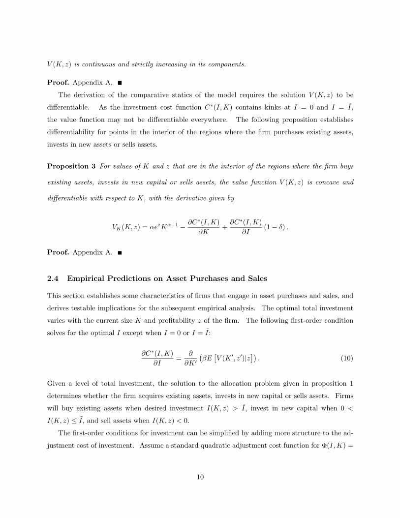
The derivation of the comparative statics of the model requires the solution V (K, z) to be

differentiable. As the investment cost function C∗(I, K) contains kinks at I = 0 and I = I,

the value function may not be differentiable everywhere. The following proposition establishes

differentiability for points in the interior of the regions where the firm purchases existing assets,

invests in new assets or sells assets.

Proposition 3 For values of K and z that are in the interior of the regions where the firm buys

existing assets, invests in new capital or sells assets, the value function V (K, z) is concave and

differentiable with respect to K, with the derivative given by

VK(K, z) = αezKα−1 −∂C∗(I, K)

∂K+

∂C∗(I, K)

∂I(1 − δ) .

Proof. Appendix A.

2.4 Empirical Predictions on Asset Purchases and Sales

This section establishes some characteristics of firms that engage in asset purchases and sales, and

derives testable implications for the subsequent empirical analysis. The optimal total investment

varies with the current size K and profitability z of the firm. The following first-order condition

solves for the optimal I except when I = 0 or I = I:

∂C∗(I, K)

∂I=

∂

∂K ′

(

βE[

V (K ′, z′)|z])

. (10)

Given a level of total investment, the solution to the allocation problem given in proposition 1

determines whether the firm acquires existing assets, invests in new capital or sells assets. Firms

will buy existing assets when desired investment I(K, z) > I, invest in new capital when 0 <

I(K, z) ≤ I, and sell assets when I(K, z) < 0.

The first-order conditions for investment can be simplified by adding more structure to the ad-

justment cost of investment. Assume a standard quadratic adjustment cost function for Φ(I, K) =

10

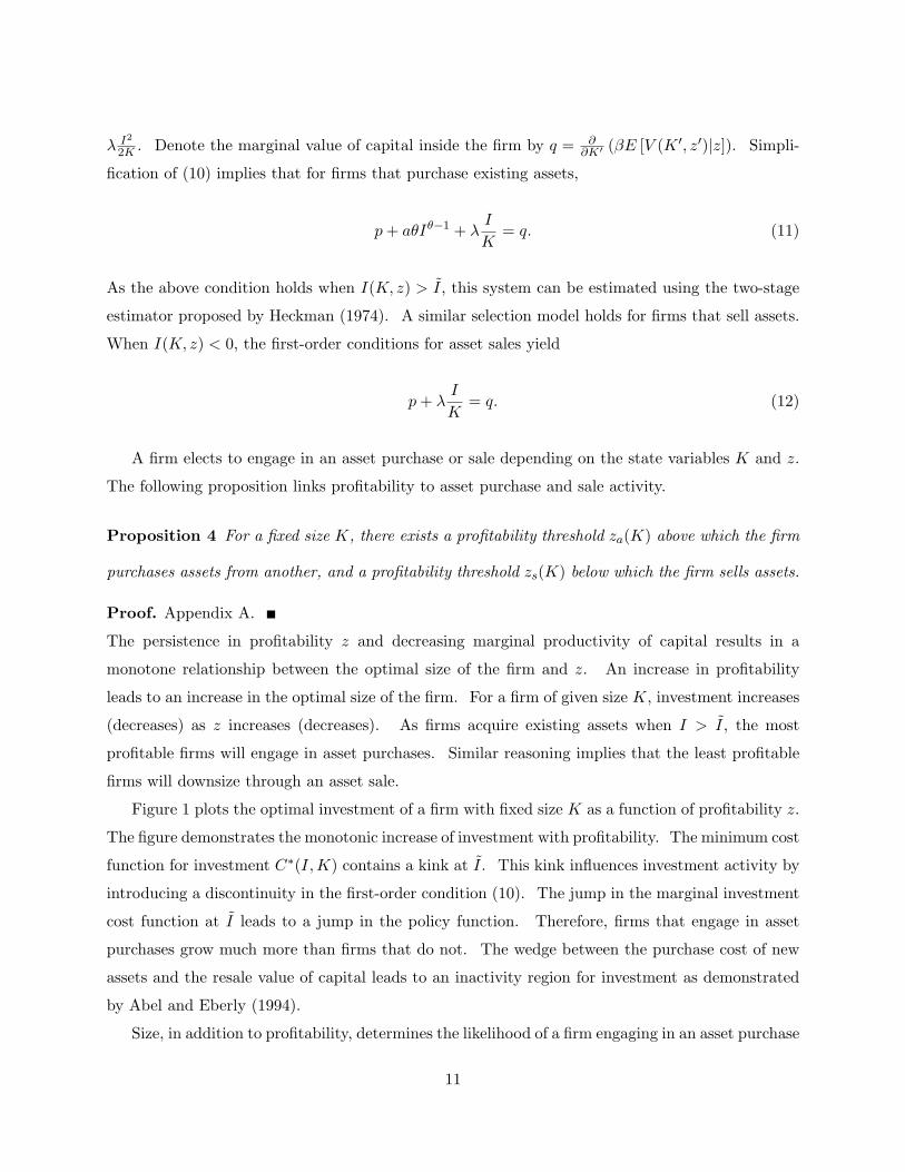
λ I2

2K . Denote the marginal value of capital inside the firm by q = ∂∂K′ (βE [V (K ′, z′)|z]). Simpli-

fication of (10) implies that for firms that purchase existing assets,

p + aθIθ−1 + λI

K= q. (11)

As the above condition holds when I(K, z) > I, this system can be estimated using the two-stage

estimator proposed by Heckman (1974). A similar selection model holds for firms that sell assets.

When I(K, z) < 0, the first-order conditions for asset sales yield

p + λI

K= q. (12)

A firm elects to engage in an asset purchase or sale depending on the state variables K and z.

The following proposition links profitability to asset purchase and sale activity.

Proposition 4 For a fixed size K, there exists a profitability threshold za(K) above which the firm

purchases assets from another, and a profitability threshold zs(K) below which the firm sells assets.

Proof. Appendix A.

The persistence in profitability z and decreasing marginal productivity of capital results in a

monotone relationship between the optimal size of the firm and z. An increase in profitability

leads to an increase in the optimal size of the firm. For a firm of given size K, investment increases

(decreases) as z increases (decreases). As firms acquire existing assets when I > I, the most

profitable firms will engage in asset purchases. Similar reasoning implies that the least profitable

firms will downsize through an asset sale.

Figure 1 plots the optimal investment of a firm with fixed size K as a function of profitability z.

The figure demonstrates the monotonic increase of investment with profitability. The minimum cost

function for investment C∗(I, K) contains a kink at I. This kink influences investment activity by

introducing a discontinuity in the first-order condition (10). The jump in the marginal investment

cost function at I leads to a jump in the policy function. Therefore, firms that engage in asset

purchases grow much more than firms that do not. The wedge between the purchase cost of new

assets and the resale value of capital leads to an inactivity region for investment as demonstrated

by Abel and Eberly (1994).

Size, in addition to profitability, determines the likelihood of a firm engaging in an asset purchase

11

or sale. The following proposition demonstrates that larger firms are more likely to sell assets.

Proposition 5 For a given level of profitability z, there exists a size threshold Ks(z) above which

the firm sells assets.

Proof. Appendix A.

As the optimal size of the firm decreases when profitability decreases, some firms that suffer a

negative profitability shock will find themselves with more assets than optimal. These firms will

sell assets to reach the optimal size. The asset sale improves the average productivity of the

remaining assets of the firm. Large firms will be more likely to find themselves with too many

assets than optimal, and therefore will be more likely to engage in asset sales.

For most parameter values, the probability of an asset purchase will increase with firm size.10

For a given level of investment I, the constant returns to scale adjustment cost of investment lowers

the investment cost as the size of the firm increases. This captures the intuition that larger firms

integrate new assets more easily than smaller firms. As size decreases, the cost of investing more

than I increases, thereby lowering the likelihood of an asset purchase.

The determinants of firm’s decisions to engage in an asset purchase or sale can be tested using

limited dependent variable regressions. Define yi,t+1 as a variable that takes values of -1, 0 or 1

depending on whether the ith firm sells existing assets, neither buys nor sells assets or buys existing

assets from another firm during the t + 1 fiscal year.

yi,t+1 = 1 if I(Ki,t, zi,t) > I

yi,t+1 = 0 if 0 ≤ I(Ki,t, zi,t) ≤ I

yi,t+1 = −1 if I(Ki,t, zi,t) < 0

I(K, z) = β0 + β1z + β2K + ε, (13)

where ε denotes an approximation error. With additional distribution assumptions on the error

term, the above system can be estimated using ordered or multinomial logit regressions. The

next section numerically solves the model and generates a simulated panel data set of firms. The

analysis of the simulated data highlights the theoretical predictions of the model.

10The result will fail for values of I close to 0, as almost all growth will then occur through asset purchases.

12

3 Calibration and Simulation

The study of simulated data sets follows a burgeoning literature.11 This approach is particularly

beneficial when issues such as endogeneity, multi-collinearity and measurement errors cause prob-

lems for statistical analysis. This section presents the results of testing the model predictions on

a simulated data set; Section 5 replicates this analysis on the actual data.

3.1 Calibration

The calibration exercise fits the model parameters to their empirical counterparts at an annual

frequency. The calibration focuses on generating a plausible panel of firm characteristics. The

discount factor in the simulated economy β = 0.95. The decreasing returns to scale parameter

α = .9 follows Gomes (2001) and maps to capital and labor elasticities in the economy of 2/3

and 30% respectively. The depreciation rate of 12% corresponds to the rate of new investment in

the economy. The study parameterizes the adjustment costs as Φ(I, K) = λI2

2K . Whited (1992)

estimates structural investment models and obtains values for the adjustment cost parameter λ

of .5 to 2. Hall (2004) uses industry level data and obtains an estimate for λ close to 0. The

study uses a value of λ = 1. The parameters of the transition equation, θ, ρandσz, determine

the cross-sectional and time series properties of profitability. The calibrated parameters imply an

autocorrelation coefficient of .85 and an unconditional standard deviation of 30% for profitability.

The calibration of the transaction cost of asset purchases selects a value to match the observed

frequency of asset transactions in the sample. The chosen values of a = 0.02 and θ = 0 represent

approximately 8% of the annual profits of the median firm. The relative price of purchased capital

p is set such that aggregate asset purchases equal aggregate asset sales. This corresponds to the

price that clears the market for corporate assets in the stationary state of the economy. The

calibrated value of p equals 0.98. Empirically, this measures the discount at which firms transact

operating units. Pulvino (1998) provides an empirical counterpart to this value. He studies the

discount on used airplane sales, and finds no discount in good times, and a mean discount of 14%

in bad times. Cooper and Haltiwanger (2006) structurally estimate an investment model with a

discount on the resale value and obtain values of p ranging from 0.80 to 0.98 in their most general

specification. A higher value for a would imply a lower value for p and fewer transactions. A

lower value of p does not significantly impact the results of the logit regression and the investment

11Gomes and Livdan (2004), Whited (2006), among others, use simulated data sets to study firm behavior.

13

regression for buyers and sellers.

Appendix B provides details on the numerical solution of the value function and the character-

ization of the optimal investment policies. Figure 2 plots the regions in which the firm buys and

sells assets. As the model predicts, highly profitable firms engage in asset purchases, and firms

with low profitability sell assets. The profitability level below which the firm sells assets increases

with size. As firms become larger, the likelihood that their size is greater than is optimal for a

given profitability level increases, leading to an increased likelihood of an asset sale.

3.2 Simulation Results

The model sheds light on firms’ decisions to grow internally, grow through acquisitions or sell

assets. The empirical analysis focuses on testing the first-order conditions given in (11) and (12),

conditional on the selection criteria identified in propositions 4 and 5. Logit regressions on the

choice of firms to buy and sell assets identify the primary determinants of these decisions. The

selection models study the relationship between (dis)investment and Tobin’s Q, conditional on a

firm engaging in an asset purchase or sale. These regressions test the model’s predictions that

changes in profitability and investment opportunities drive asset purchases and sales.

The empirical analysis tests approximations to the optimal investment policies of the firm. The

logistic regressions linearize investment as a function of the state variables and the selection models

use average Q as a proxy for marginal Q. Performing these regressions on the simulated data

set tests the validity of these approximations, and provides a basis for the subsequent empirical

analysis. Additionally, this approach helps quantify the impact of measurement error on these

regressions.

Appendix C details the construction of the simulated data set. Panel A of Table 1 reports the

results of an ordered logit regression on asset purchases and sales for the full sample, and asset

purchases by rapidly growing firms. This regression tests the prediction of proposition 4. As

predicted by the model, there exists a clear ordering between profitability and asset purchases and

sales. Limiting the sample to firms with investment to capital greater than 25% (rapid growth

firms) leads to similar results. Conditioning on a firm entering a period of high growth, those

with higher profitability seek external growth. Columns 2 and 3 of panel A demonstrate that

the addition of noise leads to lower coefficients and pseudo R2 values. The noise was added by

interchanging 10% and 20% of firms that engaged in asset purchases and sales with a matching

number of firms that grew organically. The statistical significance of the coefficient on return on

14

assets remains robust to mixing 20% of the buyers and sellers.

Panel B reports the results of the multinomial regression for the full sample. The signs of

the coefficients on return on assets and size match those predicted by propositions 4 and 5. The

addition of noise by mixing the participants drives the coefficients towards zero and lowers the

pseudo R2 values. However, the coefficients retain their sign and statistical significance. This

indicates that even in the presence of random mixing, one would find a robust relationship between

profitability, size and asset purchases and sales.

Panel C reports the results of testing the investment regression for asset purchases and sales on

the full sample as well as for asset purchases by rapidly growing firms. The strongly significant

coefficient on Tobin’s Q demonstrates that average Q functions as a good proxy for marginal Q in

the simulated data. This finding extends to limiting the sample to firms with capital expenditures

above 25%.12 The positive coefficient on cash flow supports the argument of Cooper and Ejarque

(2003) that market power, as captured by decreasing returns to scale in profitability, leads to a

positive coefficient on cash flow for investment regressions. However, adding cash flow has almost

no impact on the R2 value for both the asset purchase regressions. The next section presents the

actual data used to test the model.

4 Data

The data on asset purchases and sales is obtained from the SDC Platinum mergers and acquisitions

database. Thomson Financial Services Ltd. maintains the data set, which contains detailed infor-

mation on purchases and sales of operating units by firms. The data categorizes each transaction

as a merger, an acquisition, an asset acquisition or an acquisition of certain assets. The sample of

asset purchases and sales in the study consists of transactions listed in the last two categories. The

value of the transaction is available for about half of the sample. The selected sample consists of all

buyers and sellers from 1985 to the end of 2005, who are either publicly listed firms or subsidiaries

of listed companies.13 The sample includes transactions where one of the parties is a private firm.

The selection scheme yields a comprehensive list of firms who have elected to grow or shrink via

asset purchases and sales.

The Compustat annual files and the CRSP monthly stock files provide information on the

12Most asset purchases in the simulated data are associated with capex above 25%.13Discussions with an SDC employee verified that the data set provides comprehensive coverage on such transactions

from 1985 onwards.

15

operating performance and market valuation of firms. These are linked to the SDC sample via

the CUSIP numbers of the participants, or for transactions by subsidiaries, the CUSIP numbers of

their listed parents. The sample is categorized according to the Fama-French 48 industry groups

and excludes all financial firms and regulated utilities. This yields a panel of firms that can be

used to study the determinants of firms’ decisions to buy or sell business units. The median

transaction size in the sample is $14.6 million. The study constructs the following independent

variables at the end of each fiscal year: return on assets (RoA) equals earnings before interest,

depreciation and taxes scaled by book assets at the beginning of the period; size is the log of the

book value of assets; finance Q is the ratio of market value of assets14 to the book value of assets;

market-to-book is the ratio of market value of equity to the book value of equity; leverage is the

book value of debt divided by book value of debt plus equity; sales growth measures the growth

in net sales over the previous year; plant, property, and equipment (PPE) growth measures the

change in net plant, property and equipment over the previous fiscal year; stock return measures

the return over the fiscal year; and cash is the value of cash and short-term instruments scaled by

book assets. Sales growth and PPE growth are adjusted for inflation using the deflator for gross

private investment. Additionally, an asset purchase wave dummy variable is constructed following

the method employed by Harford (2005). A wave dummy value of 1 corresponds to a heightened

period of activity for each industry over a two year time period. The wave dummy variable takes

a value of 1, if in the two year period with the maximum number of transactions, that number is

greater than the 95th percentile obtained by simulating draws from an uniform distribution. The

study also reports results using industry means of market-to-book, leverage, sales growth, PPE

growth, stock return and cash to mitigate endogeneity concerns.

Measurement error in average Q affects statistical inference on both the Q coefficient as well as

other coefficients. The finance Q measure, popular in the corporate finance literature, focuses on the

market to book value of all assets employed by the firm. Erickson and Whited (2006) demonstrates

that macro Q measures have less measurement error than finance Q measures. Macro Q equals

the ratio of the market value of the capital stock to its replacement value. This study computes

the replacement value of capital using the perpetual inventory method of Salinger and Summers

(1983). The market value of capital equals common equity + preferred equity + debt - inventories

- cash.15 The macro Q regressions drop observations with Q values less than 0 or greater than 20.

14Market value of assets is defined as market value of equity + book assets - book equity - deferred taxation.15Common equity is measured at market value. Other values are at measured at book value. This derivation follows

Gomes (2001) except for the substraction of cash holdings from firm value to obtain the market value of capital.

16

Potential errors in the SDC database can impact the results of the empirical analysis.16 The

study relies on SDC to identify the participants, the transaction value and the fiscal year. A

detailed search using Factiva on 498 asset purchases yielded information on 388 transactions. Of

these, 343 (88% of the sample) had deal values within 5% of the value reported in the SDC. There

were 8 transactions whose reported values differed by 50% or more. SDC reported the buyer

as the seller and vice versa for 8 transactions. The SDC dates were accurate within a business

day for 92% of the sample. These findings indicate that data errors in the SDC sample on asset

transactions are relatively small and would not materially impact statistical inference.

4.1 Summary Statistics

Table 2 reports sample statistics for all firms listed on Compustat from 1984 to 2004, and for

the subsample of buyers and sellers of existing assets in the year prior to the transaction. On

average, 12% of all listed firms will buy assets from another firm, and 5% of firms will sell. As the

model predicts, buyers tend to have a higher return on assets than other firms. This suggests that

managers of firms with high profitability elect to grow through an asset purchase. Sellers have a

higher mean and lower median return on assets than other firms. Both buyers and sellers are larger

than the average firm. Large firms will be more likely to have exhausted their internal growth

opportunities and may seek to expand through an acquisition. A large firm will also find it easier

to integrate an acquired unit. On the other hand, a troubled large firm can improve profitability

by selling an underperforming unit to another firm.

The market values buyers more and sellers less than average firms when market-to-book ratios

and finance and macro Q values are used as metrics. Acquiring firms may exercise their growth

options through the purchase of relatively inefficient units of other firms. Acquiring firms have

been growing rapidly in the year prior to the transaction. They exhibit significantly higher sales

growth, and net plant, property and equipment growth than the average firm. Sellers, on the other

hand, demonstrate anemic growth prior to the transaction.

Selling firms demonstrate some evidence of financial distress. Both buyers and sellers have

less cash than average firms, but this is more pronounced for sellers. Some selling firms may face

liquidity problems, and sell units to raise cash. This would be consistent with the arguments of

Lang, Poulson, and Stulz (1995). Sellers also have higher leverage than average firms, increasing

the potential costs of obtaining new funds in the bond market. The next section test the predictions

16See Ljungqvist and Wilhelm (2003) for a discussion of SDC errors regarding IPO issuance.

17

of the model using this data set and compares the findings to those obtained with the simulated

data set.

5 Evidence on Asset Purchases and Sales

The empirical implementation tests two hypotheses derived from the above model. Hypothesis 1

states that large firms with high profitability grow by acquiring assets and that large firms with low

profitability sell assets. An alternative hypothesis, based on agency arguments, states that large

firms with high free cash flow acquire existing assets whereas firms with lower free cash flow grow

organically. Hypothesis 2 states that, conditional on a firm buying or selling assets, the quantity

of assets transacted covaries with Tobin’s Q.

Discrete choice models provide a natural method for determining the characteristics of buyers

and sellers. Hypothesis 1 predicts a monotone ordering between profitability and the choice of

a firm to sell assets, invest in new capital or buy existing assets. The next subsection tests this

prediction using an ordered logit model.

5.1 Ordered Logit Regressions

The ordered logit model estimates the limited dependent variable system given in (13). The

logit regression imposes the additional distributional assumption that the cumulative distribution

function of the error term εi,t+1 follows a logistic distribution:

F (εi,t+1) =exp(εi,t+1)

1 + exp(εi,t+1).

The empirical tests employ return on assets as a proxy for profitability, the log of book assets as a

measure of size, and use market-to-book, wave dummy, leverage, cash, stock return, sales growth

and PPE growth as control variables.

Table 3 reports the results from estimation of the above ordered logit model. The full sample

results from Panel A in Table 1 provide the simulation counterpart. Standard errors are reported in

parentheses. The regressors includes year and industry dummies. The standard error computation

clusters by firms to adjust for within-firm serial correlation and is robust to heteroskedasticity across

firms. The study evaluates statistical significance using bootstrapped finite-sample critical values

18

for the t-statistics.17 The table also reports the odds ratios corresponding to the given parameter

estimates. The odds ratios represent the relative increase in the odds in favor of an asset purchase

relative to not purchasing assets for a unit standard deviation increase in the independent variable.

The latter half of the table reports the results obtained by replacing the control variables of market-

to-book, leverage, cash, stock return, sales growth and PPE growth with their industry means. The

industry values help mitigate endogeneity concerns. The Value columns report results where the

dependent variable takes values of -1 and 1 only when SDC reports a deal value for the asset sale

or purchase. This focuses the analysis on larger and presumably more important transactions.

The regression coefficients of all covariates except cash do not vary much across either of the

two specifications for the dependent variable when using firm level controls. RoA strongly predicts

the decision of the firm to buy or sell assets. A unit standard deviation increase in RoA increases

the odds in favor of an asset purchase, and decreases the odds in favor of a sale by 26%. This

supports the prediction of the model that high z firms would buy existing assets and low z firms

would sell assets. The impact of RoA remains strong when the firm level controls are replaced by

industry counterparts. Adjusting for industry characteristics, a unit standard deviation increase in

RoA increases the odds in favor of an asset purchase by 20%. While RoA has the strongest impact

on the relative odds of a transaction, the control variables also influence the decision to engage in

an asset purchase or sale. The positive and significant coefficient on realized stock return accords

with the model intuition that positive shocks to profitability lead to asset purchases. Similarly,

the coefficients on sales growth and PPE growth demonstrate that buyers have had strong growth

while sellers have had weak growth.

The significant coefficients on cash and leverage demonstrate that the model does not capture

all the determinants of the choice of a firm to engage in an asset purchase or sale. Purchasers

have lower leverage and sellers higher leverage than other firms, indicating that high leverage can

deter asset purchases through reduced managerial flexibility. Endogenous leverage models, such

as Hennessy and Whited (2005), generate a similar result. In these models a high leverage firm

would be less willing to invest heavily following a positive shock as this would typically require

them to increase leverage, thereby driving the firm away from its optimum. The leverage effect

in the data extends to the industry measures. The positive coefficient on the stock of liquid

17The bootstrap critical values for the t-statistics were generated using 2000 bootstrap replications for each sample,with resampling at the firm level. The bootstrap t equals the difference between the bootstrap and actual pointestimates divided by the bootstrap standard error. The 2.5th and 97.5th percentiles of the bootstrap t-statistic yieldthe critical values for significance at the 5% level. I infer significance if the actual t-statistic falls outside the criticalvalues. See Efron and Tibshirani (1993, Chapter 12) for a detailed discussion.

19

assets demonstrates that financing considerations influence asset purchase or sale decisions. The

ordered logit regressions implicitly assume that the independent variables have the same impact

on the asset purchase and sale decisions. This restriction leads to a low pseudo R-square value for

the regression. The next section reports the results of multinomial regressions on the same data

set. This specification allows the covariates to have a different impact on the purchase and sale

decisions, and provides a more thorough test of hypothesis 1.

5.2 Multinomial Logit Regressions

The multinomial regressions model the choice of a firm purchasing existing assets versus investing

in new capital conditional on not selling assets as following a standard logit model. The probability

model specifies that

Prob(yi,t+1 = 1|yi,t+1 ≥ 0) =exp (β1xi,t)

1 + exp (β1xi,t).

Where xi,t denotes a vector of predetermined covariates. A similar probabilistic model yields the

conditional probability of a firm selling assets given that it does not buy assets. The empirical

implementation includes the predetermined firm and industry control variables in the ordered logit

regression.

Table 4 reports the results from estimation of the above multinomial logit model for asset

purchases and sales. Standard errors are reported in parentheses. The analysis includes year

and industry dummies. The standard error computation clusters by firms to adjust for within-

firm serial correlation and is robust to heteroskedasticity across firms. Statistical significance

is evaluated using bootstrapped critical values for the t-statistics. The table also reports the

odds ratios corresponding to the given parameter estimates. The first half of the table reports

the coefficients for asset purchases, while the latter half reports the results for asset sales. The

Firm and Industry columns report results using firm and industry level measures for the control

variables. The simultaneous estimation of the probability models for asset purchases and sales

yields the reported coefficients.

The results for the purchase decision support hypothesis 1 and match the findings from the

simulated data set reported in Panel B of Table 1. RoA and size positively predict the likelihood

of a firm engaging in an asset purchase, and they have a much larger impact on the decision than

the control variables. A unit standard deviation increase in RoA increases the odds in favor

of a purchase by 29%. The profitability and size of the firm has a strong impact on the asset

20

purchase decision when other firm characteristics are replaced by their industry counterparts. As

in the ordered regressions, buyers display strong returns and robust growth prior to the transaction.

This accords with the intuition of the model. The significant and negative coefficient on leverage

indicates that highly levered firms buy existing assets less frequently than firms with low leverage.

The leverage result strengthens when firm measures are replaced by industry averages. The

negative and significant coefficient on cash rejects the empire-building hypothesis that firms use

surplus cash to grow by asset purchases. These results support the contention of hypothesis 1 that

profitability and firm size determine asset purchases and sales.

The results for the sale of existing assets also support the model predictions. RoA enters

the predictive equation with a significant and negative coefficient indicating that low profitability

induces firms to sell assets. A unit standard deviation increase in profitability decreases the odds

in favor of an asset sale by 34% and 23%, respectively when firm and industry control variables are

used. Size also has a strong impact on the choice of a firm to sell assets, with large firms selling

assets more frequently than small firms. In contrast to buyers, firms that sell assets demonstrate

low realized returns, and poor sales and PPE growth prior to the asset sale. The level of liquid

assets strongly impacts the choice of a firm to sell assets. A unit standard deviation increase in

cash stocks decreases the odds in favor of an asset sale by 32%. This confirms the findings of

Lang, Poulson, and Stulz (1995) that firms in financial distress sell assets to raise funds. Evidence

of financial distress does not imply that agency considerations lead to asset sales, as financing

difficulties may coexist with efficient investment. The positive coefficient on leverage provides

further evidence in support of financial difficulties leading to asset sales. At the industry level,

none of the control variables have a significant impact on predicting asset sales.

The logit regressions identify the primary determinant of the choice of a firm to buy or sell

existing assets and provide strong support for hypothesis 1. However, one would reject the stronger

hypothesis that profitability and size solely determine asset purchases and sales. Given an asset

purchase or sale, the model also links the size of the transaction to the marginal value of capital

inside the firm. The next section employs selection models to test hypothesis 2.

5.3 Selection Models

Conditional on a firm engaging in an asset purchase, the first-order conditions given in (11) link

transaction size to the marginal Q of the firm. The empirical implementation proxies for marginal

Q with average Q. Assuming that the transaction cost of asset purchases is approximately linear

21

in the relevant region, the first order condition for asset purchases can be written as

I

K= −

p + aθ

λ+

1

λQ + ε

if I(K, z) ≥ I .

Linearization of the selection equation provides a selection model, which can be estimated using

the two-step estimator developed in Heckman (1974). The two-step approach first estimates the

selection equation and then estimates the investment equation with the inverse Mill’s ratio from the

selection model as an additional covariate. The empirical implementation of the selection model

focuses only on the transactions for which SDC reports a deal value. The value of the transaction

proxies for I in the investment equation. A similar model applies to the investment decisions of

firms that sell assets. For the asset sale regressions, I is measured as the negative of the transaction

size.

Table 5 reports the results from estimation of the investment models for the purchase and sale

of existing assets.18 The asset purchase and sales results from Panel C of Table 1 provide the

simulation counterpart. Standard errors are reported in parentheses. The statistical inference

employs bootstrapped critical values for the t-statistics. The specification for the selection and

investment equations include industry and year dummies. The variables are scaled by book assets

for the finance Q regression and replacement value of capital for the macro Q regression. Following

the investment literature, the regressors also include cash flow. The coefficients for the selection

equations, once adjusted for a scaling factor to account for the use of a probit model, closely match

the results of the multinomial regressions.

The positive and significant coefficient on Tobin’s Q for asset purchases supports hypothesis

2: the transaction size covaries positively with the firm’s Q. Conditional on engaging in an asset

purchase, a firm with a higher Q will purchase more assets. This indicates that firms engage

in asset purchases in response to changes in the productivity of capital employed by the firm.

Macro Q leads to higher point estimates than finance Q, which would be consistent with reduced

measurement error in macro Q. The asset sales regression leads to mixed findings. Using finance

Q with firm controls leads to a significantly positive point estimate, as with the simulated data.

The point estimate is insignificant for the other specifications. This may be due to the influence

of financial distress on asset sales. Alternatively, a different adjustment cost structure may break

18Hovakimian and Titman (2006) study the relationship between asset sales and cash flow regressions.

22

the link between Q and the quantity of assets sold.

Typical of investment regressions, cash flow has a positive and statistically significant coefficient.

Following Fazzari, Hubbard, and Petersen (1988), this has been interpreted as evidence of financial

constraints of firms. However, recent work by Erickson and Whited (2000) and Hennessy, Levy, and

Whited (2006) have argued that this is driven by measurement error and model misspecification.

Cooper and Ejarque (2003) demonstrate that when firms have market power, investment regressions

will lead to significant and positive coefficients on cash flow. In the context of asset purchases, a

financial constraints explanation would be less plausible, as firms that buy assets tend to have had

strong profitability and growth.

The statistically significant coefficient on the inverse Mill’s Ratio for both asset purchases and

sales demonstrates the importance of accounting for endogeneity in this regression. A regression

of transaction size on Q would lead to biased estimates in the absence of the selection term.

5.4 Large Asset Purchases by Rapidly Growing Firms

This section examines large asset purchases by firms during periods of rapid growth.19 Such an

analysis provides a more focused test on the model’s predictions regarding firms’ decisions to seek

external growth versus organic investment.

The study defines periods of rapid growth as those in which the ratio of capital expenditure

to replacement value of capital was greater than 25% or greater than twice the firm’s median

value.20 The following approaches lead to similar results: defining rapid growth with respect

to industry medians; defining investment as the change in the replacement value of capital; and

defining investment as the change in book assets scaled by book assets. Using higher thresholds

for rapid growth lead to weaker results, possibly due to the drop in sample size. The analysis

focuses on firms with assets purchases greater than 50% of the value of capital expenditures.

Table 6 presents the results of a logit regression on firms’ engaging in large asset purchases

during periods of rapid growth. The rapid growth columns in Panel A of Table 1 present the

results of a similar analysis on the simulated data set. The standard errors in parentheses adjust

for heteroskedasticity and clustering at the firm level. Statistical significance is inferred using

bootstrapped critical values for the t-statistics. As with the simulated data, firms with higher

RoA engage in large asset purchases during periods of rapid growth. The odds ratios indicate an

19I thank the referee for suggesting this analysis.20Whited (2006) defines large projects as those with the ratio of capital expenditures to total assets greater than

2, 2.5 or 3 times the firm’s median value.

23

economically meaningful impact of RoA on the asset purchase decision. While most of the control

variables have little impact, low industry leverage values encourage asset purchases. These findings

support the model’s prediction that firms with higher profitability seek external growth.

Hypothesis 2 links the level of asset purchases to the firm’s investment opportunities. Table

7 presents the results of testing this relationship for firms with large asset purchases, conditional

on a period of rapid growth. The rapid growth columns in Panel C of Table 1 report the simu-

lation counterpart to this analysis. The selection equation uses the same controls as in the logit

regressions. Statistical significance is inferred using bootstrapped critical values for the t-statistics.

The results demonstrate that, as predicted by the model, transaction size covaries with the firm’s

Q for large asset purchases. The macro Q regressions yield consistently higher point estimates

and lower p-values than finance Q regressions. Further, cash flow is not significant in any of these

specifications. Whereas the inverse Mill’s ratio is not significant using the bootstrapped critical

values, it is asymptotically significant in many of the regressions. Thus, conditional on a decision to

engage in a large asset purchase, the transaction size increases with the firm’s growth opportunities.

5.5 Robustness

The panel nature of the sample provides some challenges to the statistical analysis. A fixed-effects

logit regression estimates a binary logit model for asset purchases only on the subsample of firms

that either purchased or sold assets in at least one year. This allows for a firm-level fixed effect in

the estimation. The estimation of fixed-effects logit models for asset purchases and sales generate

similar results for RoA and size to those reported in the multinomial regressions. Replicating the

multinomial regressions for transactions with only deal values lead to similar results for RoA and

size as those reported in table 4.

The correlation pattern in the error terms may significantly influence the estimated standard

errors (see Petersen (2006)). The study reports standard errors obtained by clustering the data at

the firm level. This allows for a constant serial correlation term for the observations of the same

firm across different years. An alternative approach using the Fama and MacBeth (1973) procedure

yields similar results for the ordered and multinomial logit regressions. Such an approach would

generate standard errors robust to cross correlation across firms in a given year. The study reports

heteroskedasticity robust clustered estimates, as firm-level factors would be more likely to influence

asset purchase and sale decisions than macro variables.

Measurement error in Q can lead to unwarranted conclusions in investment regressions (see

24

Erickson and Whited (2000); and Gomes (2001)). The testable predictions of the model relate to

the coefficient on Q. Measurement error in a given regressor will bias that coefficient down towards

zero, making it harder to find statistical significance. Therefore, it is unlikely that the significant

coefficients on Q for the asset purchase regressions in tables 5 and 7 are driven by measurement

errors in Q. In the absence of measurement error, the true point estimates would be greater than

those reported in the above tables.

Measurement error in Q also affects inference on the cash flow coefficient. The proxy quality

threshold method of Erickson and Whited (2005) computes the minimum correlation between

observed and true Q required to infer positivity of another coefficient under various assumptions on

the measurement error structure. A high threshold value implies that the observed Q must be a very

good proxy for the true Q in order for the coefficient sign of interest to be robust to measurement

error. The reverse regression of Q on investment, cash flow and the inverse Mill’s ratio for asset

purchases yields positive cash flow coefficients with the finance Q and negative coefficients with the

macro Q. This indicates that, using the finance Q as the proxy for true Q, the cash flow coefficient is

positive under the classical errors-in-variables model and when the measurement error is correlated

with one or more of the regressors but not the disturbance. Proxy quality computation using

macro Q leads to thresholds around 0.20 under the above assumptions. Under the assumption

that the measurement error correlates with the disturbance but not the regressors the threshold

increases to 0.50 for the macro Q. This implies that the correlation between macro Q and the true

incentive to invest must be greater than 0.50 in order for the positive cash flow coefficient to be

robust to measurement error. Whereas the positive cash flow coefficients in Table 5 match the

simulation results, these computations demonstrate that inference on the cash flow coefficients is

sensitive to measurement error in Q (see Erickson and Whited (2000)).

The significant and positive coefficient on RoA can be interpreted in favor of an alternative

hypothesis based on agency conflicts. The agency hypothesis argues that managers derive benefits

from increased size, and use free cash flow to grow via asset purchases. High return on assets

indicates increased cash flow to the firm, and managers with misaligned incentives use the excess

cash to grow the firm and increase their private benefits. Proposition 4 demonstrates that value-

maximizing managers respond to increased profitability by engaging in asset purchases. The

replication of the above logit regressions with a free cash flow measure provides a test of the

alternative hypothesis. The free cash flow variable measures net operating cash flow minus cash

25

flow for investing activities, divided by book assets at the beginning of the fiscal year.21

Table 8 presents the results of estimating the multinomial logit regression using free cash flow

in place of RoA. The coefficient on free cash flow itself is statistically insignificant as a predictor

of asset purchases, and significantly negative as a predictor of asset sales. This provides evidence

that high free cash flow does not lead to asset purchases, and indicates that the impact of RoA

on asset purchases does not capture a free cash flow effect. These findings demonstrate that one

can reject the alternative hypothesis on asset purchases based on agency arguments. Overall, the

empirical evidence supports the two efficiency based hypotheses on asset purchases and sales.

6 Conclusion

This study argues that decisions over the optimal scale of the firm drive organic investment, acqui-

sitions and asset sales. The paper analyzes these transactions in the context of an efficiency based

model: asset purchases and sales help firms move towards their optimal size after heterogenous pro-

ductivity shocks. Conditional on a firm buying or selling existing assets, the model links purchases

and sales of existing assets to the marginal value of capital inside the firm. The profitability and

size of the firm determines whether the firm chooses to buy or sell existing assets.

The paper tests the implications of the model using a data set of asset purchases and sales from

the SDC Platinum database. The estimation of the selection models for investment demonstrates

a positive link between the quantity of assets purchased and the investment opportunities of the

firm. Return on assets and size strongly predict the likelihood of a firm engaging in an asset

purchase or sale. A unit standard deviation increase in RoA increases the probability of an asset

purchase by 29%, while a corresponding decrease in RoA increases the likelihood of an asset sale

by 34%. Focusing the analysis on large asset purchases by firms during periods of rapid growth

yields similar results. The empirical analysis also finds that financing considerations influence the

decision of firms to sell assets, with lower levels of liquid assets leading to more asset sales. On

the other hand, increased cash stocks do not lead to increased asset purchases, indicating that

empire-building tendencies do not influence asset purchases.

The findings on asset purchases contrast with the evidence linking agency problems and misval-

uations to mergers. Further research on the sources and effects of the differences between mergers

21Net operating cash flow and net investing cash flow are given by Compustat variables 308 and 311, respectively:Free cash flow = data308 + data311. Free cash flow measures the cash generated from operations net of investmentactivity. These variables are available from 1987 onwards.

26

and asset purchases may prove fruitful, given that the fundamental action of both transactions is

to shift ownership of some productive assets from one firm to another.

27

Appendix

A Proofs

Proposition 1 There exists a threshold I =[

a1−p

]1/(1−θ)below which all investment consists of

new investment and above which all investment consists of purchased existing capital

I = N if 0 ≤ I ≤ I (A.1)

= M if I < 0 or I > I.

Corollary The investment cost function C∗(I, K) obtained by substitution of the above allocation

choice is continuous.

Proof. The differentiation of (5) yields the first-order conditions for optimality:

∂C

∂N= 1 +

∂Φ(I, K)

∂I∂C

∂M= p +

∂Φ(I, K)

∂I+ aθM θ−1 · 1(M>0).

There does not exist an interior solution to the problem. The boundary conditions imply that

C(I , 0, K) = C(0, I, K).

The solution to the above equation yields that I =[

a1−p

]1/(1−θ). As asset purchases have a

lower marginal cost of investment for I ≥ I, (p + (1 − p)θ < 1), the firm will buy assets. The

transaction cost of asset purchases Ψ(M) leads firms to grow via new investment for 0 < I < I.

By construction, all disinvestment enters the model as M . This establishes the allocation choices

given above in (A.1).

The following equation yields the minimum cost of an investment of I at current capital K:

C∗(I, K) = I + Φ(I, K) − (1 − p)I · 1(I<0 or I>I) + aIθ · 1(I>I). (A.2)

28

Substitution of the optimal allocation to asset purchases, new investment and asset sales to the

investment cash flow equation given in (5) yields the investment cost function (A.2). The continuity

of C∗(I, K) over K and at points in the interior of the investment regions follows trivially. The

continuity of the function at I follows from the value matching condition to the allocation problem.

Taking left and right limits of C∗(I, K) as I → 0, one obtains

limI→0−

C∗(I, K) = limI→0+

C∗(I, K) = 0.

This establishes continuity of C∗(I, K) at 0. Therefore, C∗(I, K) is continuous on its domain.

Proposition 2 There exists a unique function V (K, z) that solves for the current value of the firm.

V (K, z) is continuous and strictly increasing in its components.

Proof. The return function F (K, z) − C∗(I, K) is continuous. Therefore, assumptions 9.4 - 9.7

of Stokey and Lucas (1989) hold. Theorem 9.6 yields the existence and uniqueness of the value

function V (K, z). The return increases with the current level of capital K. Assumptions 9.8 and

9.9 of Stokey and Lucas (1989) hold, and Theorem 9.7 yields that the value function is strictly

increasing in K. Similarly, Theorem 9.11 of Stokey and Lucas (1989) yields that the value function

is strictly increasing in z.

Proposition 3 For values of K and z that are in the interior of the regions where the firm buys

existing assets, invests in new capital or sells assets, the value function V (K, z) is concave and

differentiable with respect to K, with the derivative given by

VK(K, z) = αezKα−1 −∂C∗(I, K)

∂K+

∂C∗(I, K)

∂I(1 − δ). (A.3)

Proof. Within each region, the return function F (K, z) − C∗(I, K) is concave and differentiable.

Theorem 9.8 of Stokey and Lucas (1989) implies strict concavity of V (K, z) at any point (K0, z0)

in the interior of these regions. Theorem 1 of Benveniste and Scheinkman (1979) implies differen-

tiability of V (K, z) and yields the above derivative.

Proposition 4 For a fixed size K, there exists a profitability threshold za(K) above which the firm

purchases assets from another, and a profitability threshold zs(K) below which the firm sells assets.

29

Proof. Fix size K. The first-order conditions for optimality yields

∂C∗(I, K)

∂I= βE

[

∂V (K(1 − δ) + I, z′)

∂I|z

]

. (A.4)

In the interior points, the partial derivative of the investment cost function is the following:

∂C∗(I, K)

∂I= 1 +

∂Φ(I, K)

∂I− (1 − p) · 1(I<0 or I>I) + aθI(θ−1) · 1(I>I). (A.5)

First consider two firms that buy assets, with profitability levels z1 and z2. Assume that z2 > z1.

Denote the associated optimal investment levels by I1 and I2. The first-order conditions yield

p +∂Φ(I1, K)

∂I+ aθI

(θ−1)1 = βE

[

∂V (K(1 − δ) + I1, z′)

∂I|z1

]

p +∂Φ(I2, K)

∂I+ aθI

(θ−1)2 = βE

[

∂V (K(1 − δ) + I2, z′)

∂I|z2

]

.

Monotonocity of the transition function for z implies that

E

[

∂V (K(1 − δ) + I2, z′)

∂I|z2

]

> E

[

∂V (K(1 − δ) + I2, z′)

∂I|z1

]

.

Substituting the F.O.C. conditions to the above inequality yields

E

[

∂V (K(1 − δ) + I1, z′)

∂I|z1

]

−∂Φ(I1, K)

∂I− aθIθ−1

1 >

E

[

∂V (K(1 − δ) + I2, z′)

∂I|z1

]

−∂Φ(I2, K)

∂I− aθIθ−1

2 . (A.6)

A proof by contradiction establishes that I2 > I1. Assume that I2 ≤ I1. Then, concavity of the

value function and convexity of the adjustment cost function imply the following inequality:

E

[

∂V (K(1 − δ) + I1, z′)

∂I|z1

]

−∂Φ(I1, K)

∂I− aθIθ−1

1 ≤

E

[

∂V (K(1 − δ) + I2, z′)

∂I|z1

]

−∂Φ(I2, K)

∂I− aθIθ−1

2 .

This contradicts (A.6). Therefore I2 > I1. The proof requires a low marginal transaction cost

30

(a < λKθ(1−θ)

when ∂Φ(I,K)∂I = λI

K ).

A similar proof establishes that for two firms both of which either sell assets or invest in new

capital, the firm with higher profitability will invest more (z2 > z1 ⇒ I2 > I1). Investment

increases monotonically with z, and a firm buys assets if I > I and sells assets when I < 0. This

establishes the proposition.

Proposition 5 For a given level of profitability z, there exists a size threshold Ks(z) above which

the firm sells assets.

Proof. Fix profitability z. Consider a firm with capital K1 that optimally engages in asset sales,

and another firm with capital K2 > K1. The result requires that I2 < 0. Assuming that these

are in the interior of the action regions, the first-order conditions imply

p +∂Φ(I1, K1)

∂I= βE

[

∂V (K1(1 − δ) + I1, z′)

∂I|z

]

(A.7)

p +∂Φ(I2, K2)

∂I≤ βE

[

∂V (K2(1 − δ) + I2, z′)

∂I|z

]

.

The constant returns to scale assumption implies that ∂Φ(I,K)∂I is an increasing function of I

K . A

proof by contradiction establishes that I2 < 0. Assume that I2 ≥ 0. Therefore I1K1

≤ I2K2

. This

implies that∂Φ(I1, K1)

∂I≤

∂Φ(I2, K2)

∂I.

Substituting the above into the F.O.C.s given in (A.7), one obtains:

E

[

∂V (K1(1 − δ) + I1, z′)

∂I|z

]

≤ E

[

∂V (K2(1 − δ) + I2, z′)

∂I|z

]

.

The concavity of the value function implies that

K1(1 − δ) + I1 ≥ K2(1 − δ) + I2

I1 ≥ (K2 − K1)(1 − δ) + I2.

Therefore I1 ≥ 0. This contradicts the initial assumption of an asset sale.

31

B Numerical Solution

The numerical solution employs value function iteration over a grid of values for current capital,

investment and profitability. The capital grid consists of 500 equally spaced points, while the

investment grid contains 5000 points. The Tauchen and Hussey (1991) approximation for AR(1)

processes yields the grid of values for profitability. This grid contains 10 points. The solution uses

the optimal allocation choices derived as the solution to (9). The solution yields an optimal policy

for new investment, asset purchases and asset sales. For a given level of capital, the transaction

costs of asset purchases lead to an upper and lower bound for profitability beyond which the firm

buys and sells assets, respectively. These bounds follow a smooth function as K varies. The

acquisition boundary for a given capital level is approximated by the interpolated value of z, which

yields an optimal total investment of I. The mid-point of the profitability levels over which the

firm begins to disinvest yields the approximate sale threshold. These values act as inputs to a

polynomial approximation of the acquire and sell thresholds as a function of log(K). The solution

uses a second-order approximation with Hermite polynomials. Within each action region, linear

interpolation provides the investment decisions and firm values.

C Simulations

The simulations apply the policy functions derived above to a panel of firms. The simulated

sample consists of 1000 firms over 100 time periods. The simulation employs the boundaries for

asset purchases and sales obtained in the numerical solution. The initial 20 periods function as

a burn-in sample. The sequence of solutions to the value function and simulation iterates until

the equilibrium value of p at which total demand for asset purchases equals total asset sales is

obtained. This corresponds to the steady state of the economy, where the inter-firm assets market

clears. Hopenhayn (1992) provides the theoretical foundation for this approach.

32

References

Abel, Andrew, 1983, Optimal investment under uncertainty, American Economic Review 73, 228–

233.

Abel, Andrew, and Janice C. Eberly, 1994, A unified model of investment under uncertainty,

American Economic Review 84, 1369–1384.

Alexander, Gordon J., George P. Bensen, and Joan M. Kampmeyer, 1984, Investigating the valua-

tion effects of announcements of voluntary corporate selloffs, Journal of Finance 39, 502–517.

Andrade, Gregor, Mark Mitchell, and Erik Stafford, 2001, New evidence and perspectives on merg-

ers, Journal of Economic Perspectives 15, 103–120.

Bates, Thomas W., 2005, Asset sales, investment opportunities, and the use of proceeds, Journal

of Finance 60, 105–135.

Benveniste, L. M., and Jose A. Scheinkman, 1979, On the differentiability of the value function in

dynamic models of economics, Econometrica 47, 727–732.

Bruner, Robert F., 2004, Applied mergers & acquisitions. (John Wiley and Sons, Inc. New Jersey,

NJ).

Caballero, Ricardo J., and Eduardo M.R.A. Engel, 1999, Explaining investment dynamics in U.S.

manufacturing: A generalized (S,s) approach, Econometrica 67, 783–826.

Colak, Gonul, and Toni M. Whited, 2005, Spin-offs, divestitures and conglomerate investment,

forthcoming, Review of Financial Studies.

Cooper, Russell W., and Joao Ejarque, 2003, Financial frictions and investment: Requiem in Q,

Review of Economic Dynamics 6, 710–728.

Cooper, Russell W., and John Haltiwanger, 2006, On the nature of capital adjustment costs, Review

of Economic Studies 73, 611–633.

Dong, Ming, David Hirshleifer, Scott Richardson, and Siew Hong Teoh, 2006, Does investor mis-

valuation drive the takeover market?, Journal of Finance 61, 725–762.

Efron, Bradley, and Robert Tibshirani, 1993, An Introduction to the Bootstrap. (Chapman and

Hall, New York, NY).

33

Eisfeldt, Andrea L., and Adriano Rampini, 2006a, Capital reallocation and liquidity, Journal of

Monetary Economics 53, 369–399.

Eisfeldt, Andrea L., and Adriano Rampini, 2006b, New or used? Investment with credit constraints,

Working paper, Northwestern University.

Erickson, Timothy, and Toni M. Whited, 2000, Measurement error and the relationship between

investment and q, Journal of Political Economy 108, 1027–1057.

Erickson, Timothy, and Toni M. Whited, 2005, Proxy-quality thresholds: Theory and applications,

Financial Research Letters 2, 131–151.

Erickson, Timothy, and Toni M. Whited, 2006, On the accuracy of different measures of q, Financial

Management 35, 5–33.

Fama, Eugene F., and James D. MacBeth, 1973, Risk, return, and equilibrium: Empirical tests,

Journal of Political Economy 81, 607–636.

Fazzari, Steven M., R. Glenn Hubbard, and Bruce C. Petersen, 1988, Financing constraints and

corporate investment, Brookings Papers on Economic Activity 1, 141–195.

Gomes, Joao, and Dmitry Livdan, 2004, Optimal diversification: Reconciling theory and evidence,

Journal of Finance 59, 507–535.

Gomes, Joao F., 2001, Financing investment, American Economic Review 90, 1263–1285.

Grossman, Sanford J., and Oliver D. Hart, 1986, The costs and benefits of ownership: A theory of

vertical and lateral integration, Journal of Political Economy 94, 691–719.

Hall, Robert E., 2004, Measuring factor adjustment costs, Quarterly Journal of Economics 119,

899–927.

Harford, Jarrad, 2005, What drives merger waves?, Journal of Financial Economics 77, 529–560.

Hart, Oliver D., and John Moore, 1990, Property rights and the nature of the firm, Journal of

Political Economy 98, 1119–1158.

Hayashi, Fumio, 1982, Tobin’s marginal and average q : A neoclassical interpretation, Econometrica

50, 213–224.

34

Heckman, James J., 1974, Shadow prices, market wages, and labor supply, Econometrica 42, 679–

694.

Hennessy, Christopher A., Amnon Levy, and Toni M. Whited, 2006, Testing Q theory with financing

frictions, forthcoming, Journal of Financial Economics.

Hennessy, Christopher A., and Toni M. Whited, 2005, Debt dynamics, Journal of Finance 60,

1129–1165.

Hite, Gailen L., James E. Owers, and Ronald C. Rogers, 1987, The market for interfirm asset sales,

Journal of Financial Economics 18, 229–253.

Hopenhayn, Hugo A., 1992, Entry, exit, and firm dynamics in long run equilibrium, Econometrica

60, 1127–1150.

Hovakimian, Gayane, and Sheridan Titman, 2006, Corporate investment with financial constraints:

Sensitivity of investment to funds from voluntary asset sales, Journal of Money, Credit and

Banking 38, 357–374.

Jain, Prem C., 1985, The effect of voluntary sell-off announcements on shareholder wealth, Journal

of Finance 40, 209–223.

John, Kose, and Eli Ofek, 1995, Asset sales and increase in focus, Journal of Financial Economics

37, 105–126.

Jovanovic, Boyan, and Peter Rousseau, 2002, The Q-theory of mergers, American Economic Review

(Papers and Proceedings) 92, 198–204.

Klein, Benjamin, Robert G. Crawford, and Armen A. Alchian, 1978, Vertical integration, appropri-

able rents, and the competitive contracting process, Journal of Law and Economics 21, 297–326.

Lang, Larry H. P., Annette B. Poulson, and Rene M. Stulz, 1995, Asset sales, firm performance,

and the agency costs of managerial discretion, Journal of Financial Economics 37, 3–37.

Ljungqvist, Alexander, and William J. Wilhelm, Jr., 2003, IPO pricing in the dot-com bubble,

Journal of Finance 58, 723–752.

Loughran, Tim, and Anand Vijh, 1997, Do long-term shareholders benefit from corporate acquisi-

tions?, Journal of Finance 52, 1765–1790.

35

Lucas, Robert E., Jr., 1967, Adjustment costs and the theory of supply, Journal of Political Econ-

omy 75, 321–334.

Maksimovic, Vojislav, and Gordon Phillips, 2001, The market for corporate assets: Who engages

in mergers and asset sales and are there efficiency gains?, Journal of Finance 56, 2019–2065.

Maksimovic, Vojislav, and Gordon Phillips, 2002, Do conglomerates allocate resources efficiently?,

Journal of Finance 57, 721–767.

Moeller, Sara B., Frederik P. Schlingemann, and Rene M. Stulz, 2005, Wealth destruction on a

massive scale? A study of acquiring-firm returns in the recent merger wave, Journal of Finance

60, 757–782.

Petersen, Mitchell A., 2006, Estimating standard errors in finance panel data sets: Comparing

approaches, Working paper, Northwestern University.

Pulvino, Todd C., 1998, Do asset fire sales exist? An empirical investigation of commercial aircraft

transactions, Journal of Finance 53, 939–978.

Ramey, Valerie A., and Matthew D. Shapiro, 2001, Displaced capital: A study of aerospace plant

closings, Journal of Political Economy 109, 958–992.

Ray, Sugata, and Missaka Warusawitharana, 2007, Comparing the gains from mergers and asset

purchases, Working paper, Board of Governors of the Federal Reserve.

Rhodes-Kropf, M., D. T. Robinson, and S. Viswanathan, 2005, Valuation waves and merger activity:

The empirical evidence, Journal of Financial Economics 77, 561–603.

Salinger, Michael A., and Lawrence H. Summers, 1983, Tax reform and corporate investment: A

microeconometric simulation study, in Martin Feldstein, eds.: Behavioral simulation methods in

tax policy analysis (University of Chicago Press, Chicago, IL ).

Schlingemann, Frederik P., Rene M. Stulz, and Ralph A. Walkling, 2002, Divestitures and the

liquidity of the market for corporate assets, Journal of Financial Economics 64, 117–144.

Schoar, Antoinette, 2002, Effects of corporate diversification on productivity, Journal of Finance

57, 2379–2403.

36

Slovin, Myron B., Marie E. Sushka, and John A. Poloncheck, 2005, Methods of payment in asset

sales: Contracting with equity versus cash, Journal of Finance 60, 2385–2407.

Stokey, Nancy L., and Robert E. Lucas, Jr., 1989, Recursive Methods in Economic Dynamics.

(Harvard University Press, Cambridge, MA).

Tauchen, George, and Robert Hussey, 1991, Quadrature-based methods for obtaining approximate

solutions to nonlinear asset pricing models, Econometrica 59, 371–396.

Whited, Toni M., 1992, Debt, liquidity constraints, and corporate investment: Evidence from panel

data, Journal of Finance 47, 1425–1460.

Whited, Toni M., 2006, External finance constraints and the intertemporal pattern of intermittent

investment, Journal of Financial Economics 81, 467–502.

Williamson, Oliver E., 1975, Markets and hierarchies: Analysis and antitrust implications. (Free

Press New York).

Yang, Liu, 2006, The real determinants of asset sales, Working paper, University of California, Los

Angeles.

37

Table 1: Logit Regressions and Investment Regressions on Simulated Data

The table presents the results obtained by estimating the logit regressions on assetpurchases and sales, and the investment regressions on transaction size using thesimulated data set. Section 3 details the construction of simulated data set. PanelA presents the results of the ordered logit for all firms and those with investment tocapital > 25% (rapid growth firms). Panel B presents the results of the multinomiallogit for all firms. In each case, the noise columns demonstrate the impact of addingrandom noise to the sample. The noise is added by mixing 10% and 20% of thepurchase and sale firms with the firms that invest in new capital. Panel C reportsthe results of using selection models to estimate the first order conditions for assetpurchases and sales by all firms, and asset purchases by rapid growth firms. In eachtable, standard errors are reported in parentheses.

Panel A: Ordered Logit Regressions

All firms Rapid growthSample 10% Noise 20% Noise Sample 10% Noise 20% Noise

Return on Assets 4.46 3.77 3.20 12.23 7.64 5.63(0.07) (0.07) (0.07) (0.34) (0.21) (0.17)

Observations 80000 80000 80000 16245 16245 16245Pseudo R-square 0.15 0.11 0.08 0.66 0.47 0.34

Panel B: Multinomial Logit Regressions

Purchases SalesSample 10% Noise 20% Noise Sample 10% Noise 20% Noise

Return on Assets 14.40 8.57 6.62 -2.78 -1.59 -1.04(0.32) (0.16) (0.12) (0.13) (0.11) (0.09)

Size 2.52 1.57 1.08 2.34 1.62 1.20(0.03) (0.02) (0.02) (0.03) (0.02) (0.02)

Observations 80000 80000 80000 80000 80000 80000Pseudo R-square 0.49 0.36 0.26 0.49 0.36 0.26

Panel C: Investment Regression

Purchases Sales Rapid growth(1) (2) (1) (2) (1) (2)

Tobin’s Q 0.358 0.348 0.149 0.228 0.355 0.370(0.001) (0.003) (0.003) (0.002) (0.001) (0.002)

Cash Flow 0.107 2.288 -0.108(0.023) (0.018) (0.013)

Inverse Mill’s Ratio 0.012 0.033 -0.037 0.002 -0.025 -0.044(0.003) (0.005) (0.002) (0.001) (0.003) (0.003)

Observations 1550 1550 6591 6591 1508 1508Adj. R-square 0.98 0.98 0.60 0.88 0.99 0.99

38

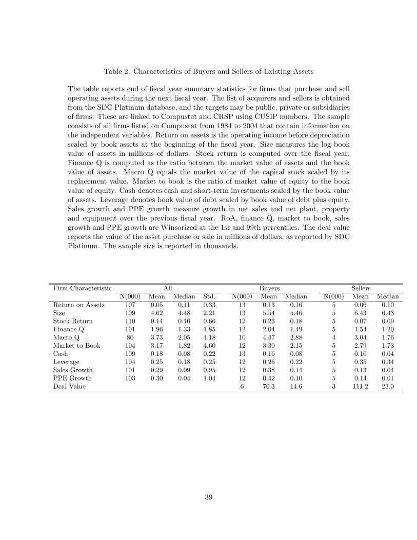
Table 2: Characteristics of Buyers and Sellers of Existing Assets

The table reports end of fiscal year summary statistics for firms that purchase and selloperating assets during the next fiscal year. The list of acquirers and sellers is obtainedfrom the SDC Platinum database, and the targets may be public, private or subsidiariesof firms. These are linked to Compustat and CRSP using CUSIP numbers. The sampleconsists of all firms listed on Compustat from 1984 to 2004 that contain information onthe independent variables. Return on assets is the operating income before depreciationscaled by book assets at the beginning of the fiscal year. Size measures the log bookvalue of assets in millions of dollars. Stock return is computed over the fiscal year.Finance Q is computed as the ratio between the market value of assets and the bookvalue of assets. Macro Q equals the market value of the capital stock scaled by itsreplacement value. Market to book is the ratio of market value of equity to the bookvalue of equity. Cash denotes cash and short-term investments scaled by the book valueof assets. Leverage denotes book value of debt scaled by book value of debt plus equity.Sales growth and PPE growth measure growth in net sales and net plant, propertyand equipment over the previous fiscal year. RoA, finance Q, market to book, salesgrowth and PPE growth are Winsorized at the 1st and 99th percentiles. The deal valuereports the value of the asset purchase or sale in millions of dollars, as reported by SDCPlatinum. The sample size is reported in thousands.

Firm Characteristic All Buyers SellersN(000) Mean Median Std. N(000) Mean Median N(000) Mean Median

Return on Assets 107 0.05 0.11 0.33 13 0.13 0.16 5 0.06 0.10Size 109 4.62 4.48 2.21 13 5.54 5.46 5 6.43 6.43Stock Return 110 0.14 0.10 0.66 12 0.23 0.18 5 0.07 0.09Finance Q 101 1.96 1.33 1.85 12 2.04 1.49 5 1.54 1.20Macro Q 80 3.73 2.05 4.18 10 4.47 2.88 4 3.04 1.76Market to Book 104 3.17 1.82 4.60 12 3.30 2.15 5 2.79 1.73Cash 109 0.18 0.08 0.22 13 0.16 0.08 5 0.10 0.04Leverage 104 0.25 0.18 0.25 12 0.26 0.22 5 0.35 0.34Sales Growth 101 0.29 0.09 0.95 12 0.38 0.14 5 0.13 0.04PPE Growth 103 0.30 0.04 1.04 12 0.42 0.10 5 0.14 0.01Deal Value 6 70.3 14.6 3 111.2 23.0

39

Table 3: Ordered Logit Regression for Purchase and Sale of Existing Assets

The table represents the results from an ordered logit regression of the choice of a firmto purchase or sell existing assets:

Pr(yi,t+1 = 1) =exp(at + βxi,t)

1 + exp(at + βxi,t).

The dependent variable (yi,t+1) equals one if the firm or a subsidiary acquired someoperations, minus one if the firm or a subsidiary sold assets, and zero otherwise. Thelist of purchasers and sellers is obtained from the SDC Platinum database, and theparticipants may be public firms or subsidiaries of public firms. The sample consistsof all firms listed on Compustat from 1984 to 2004 that contain information on theindependent variables. The independent variables are all measured at the end of theprevious fiscal year. Table 2 details the variable construction. Columns 4 and 5 reportresults replacing the control variables with their industry means. The ‘Value’ columnsfocuses only on transactions for which SDC reports a deal value. The regressionsinclude year and industry dummies. Standard errors are robust to heteroskedasticityand adjust for clustering at the firm level. The odds ratios report the increase inthe relative odds of a purchase for a firm whose independent variable increases by 1standard deviation. * and ** signify statistical significance at the 5% and 1% levelsusing bootstrapped critical values for the t-statistics.

Firm Controls Industry ControlsAll Deals Value All Deals Value

Coef. Odds Coef. Odds Coef. Odds Coef. Odds

Return on Assets 0.90** 1.26 0.96** 1.28 0.55** 1.20 0.56** 1.21(0.04) (0.05) (0.03) (0.04)

Size 0.03** 1.06 -0.002 1.00 0.01 1.02 -0.02 0.96(0.01) (0.01) (0.01) (0.01)

Wave Dummy 0.13** 1.05 0.11** 1.05 0.15** 1.06 0.14** 1.06(0.03) (0.04) (0.03) (0.04)

Stock Return 0.10** 1.07 0.10** 1.06 -0.05 0.99 -0.12 0.98(0.01) (0.02) (0.06) (0.08)

Market to Book 0.01** 1.06 0.01** 1.06 0.04* 1.05 0.05* 1.06(0.002) (0.003) (0.015) (0.019)

Leverage -0.36** 0.92 -0.25** 0.94 -1.81** 0.84 -1.78** 0.84(0.05) (0.06) (0.40) (0.49)

Cash 0.18** 1.04 0.47** 1.10 -0.16 0.98 0.43 1.05(0.05) (0.07) (0.36) (0.43)

Sales Growth 0.09** 1.08 0.10** 1.09 0.09 1.02 0.19 1.04(0.01) (0.01) (0.09) (0.11)

PPE Growth 0.07** 1.06 0.08** 1.07 0.11 1.02 0.09 1.02(0.01) (0.01) (0.07) (0.09)

Observations 86397 86397 102387 102387Pseudo R-square 0.02 0.02 0.02 0.01

40

Table 4: Multinomial Logit Regression for Purchase and Sale of Existing Assets

The table represents the results from a multinomial logit regression of the choice of afirm to purchase or sell existing assets:

Pr(yi,t+1 = j) =exp(at + βjxi,t)

1 + exp(at + βjxi,t).

The dependent variable (yi,t+1) takes three values depending on whether the firm ora subsidiary bought existing assets, sold existing assets or did neither. The tablereports the coefficients for purchasing or selling assets compared to doing neither. Thelist of purchasers and sellers is obtained from the SDC Platinum database, and theparticipants may be public firms or subsidiaries of public firms. The sample consistsof all firms listed on Compustat from 1984 to 2004 that contain information on theindependent variables. The independent variables are all measured at the end of theprevious fiscal year. Table 2 details the variable construction. Columns 3 and 5 reportresults replacing the control variables with their industry means. The regressionsinclude year and industry dummies. Standard errors are robust to heteroskedasticityand adjust for clustering at the firm level. The odds ratios report the change in therelative odds of a purchase or a sale for a firm whose independent variable increases by1 standard deviation. * and ** signify statistical significance at the 5% and 1% levelsusing bootstrapped critical values for the t-statistics.

Purchases SalesFirm Industry Firm Industry

Coef. Odds Coef. Odds Coef. Odds Coef. Odds

Return on Assets 1.00** 1.29 0.70** 1.27 -1.64** 0.66 -0.78** 0.77(0.08) (0.07) (0.07) (0.04)

Size 0.25** 1.73 0.23** 1.66 0.44** 2.57 0.44** 2.66(0.01) (0.01) (0.01) (0.01)

Wave Dummy 0.12** 1.05 0.14** 1.06 -0.04 0.99 -0.07 0.97(0.03) (0.03) (0.05) (0.05)

Stock Return 0.11** 1.08 0.04 1.01 -0.11** 0.93 0.18 1.04(0.02) (0.08) (0.03) (0.11)

Market to Book 0.02** 1.08 0.06** 1.08 0.01 1.04 0.04 1.06(0.003) (0.018) (0.004) (0.025)

Leverage -0.26** 0.94 -2.19** 0.81 0.43** 1.11 -0.51 0.95(0.07) (0.48) (0.10) (0.64)

Cash -0.25** 0.95 -0.14 0.98 -1.87** 0.68 -1.20 0.88(0.09) (0.50) (0.16) (0.68)

Sales Growth 0.11** 1.10 0.04 1.01 -0.19** 0.85 -0.13 0.97(0.01) (0.12) (0.04) (0.17)

PPE Growth 0.05** 1.05 0.11 1.02 -0.12** 0.90 -0.14 0.97(0.01) (0.09) (0.04) (0.13)

Observations 86397 102387 86397 102387Pseudo R-square 0.09 0.08 0.09 0.08

41

Table 5: Investment Regression for Asset Purchases and Sales

The table reports the results from estimating the following equation:

I

K= c + a ∗ Q + b ∗ CF + ε,

conditional on the firm either purchasing or selling existing assets, where I denotes thevalue of the assets purchased or sold, Q measures either finance Q or macro Q, and CFequals cash flow. The scaling variable K equals book assets for the finance Q regressionand the replacement value of capital for the macro Q regression. The resulting modelis estimated using a Heckman two-step estimator. The selection equation includessize, return on assets, market to book, wave dummy, stock return, leverage, cash,sales growth and PPE growth as independent variables. Columns 3 and 5 presentresults with the control variables for the selection equation replaced by their industrymeans. The selection equation and the investment equation include year and industrydummies. The sample of asset purchases and sales is obtained from SDC Platinum andconsists of all asset transactions from 1985 to the end of 2005. Panel A reports theresults obtained for the purchase of assets and Panel B reports the results for the saleof assets. The tables report the number of uncensored observations. * and ** signifystatistical significance at the 5% and 1% levels using bootstrapped critical values forthe t-statistics.

Panel A: Investment Regression for Asset Purchasers

Finance Q Macro QFirm Industry Firm Industry

Tobin’s Q 0.019** 0.011** 0.029** 0.027**(0.002) (0.001) (0.002) (0.002)

Cash Flow 0.116** 0.113** 0.078** 0.085**(0.017) (0.016) (0.011) (0.010)

Inverse Mill’s Ratio 0.302** 0.340** 0.855** 0.891**(0.016) (0.017) (0.048) (0.049)

Observations 5652 6363 4344 4864Adj. R-square 0.11 0.12 0.16 0.16

Panel B: Investment Regression for Asset Sellers

Finance Q Macro QFirm Industry Firm Industry

Tobin’s Q 0.0054* 0.0008 0.0002 -0.0015(0.0021) (0.0020) (0.0010) (0.0010)

Cash Flow 0.075** 0.030** 0.009 0.009(0.010) (0.010) (0.005) (0.004)

Inverse Mill’s Ratio -0.109** -0.133** -0.108** -0.115**(0.006) (0.007) (0.007) (0.007)

Observations 2474 2626 1722 1919Adj. R-square 0.19 0.22 0.19 0.20

42

Table 6: Logit Regression for Large Asset Purchases by Rapidly Growing Firms

The table represents the results from a logit regression of the choice of a firm to purchaseexisting assets:

Pr(yi,t+1 = 1) =exp(at + βxi,t)

1 + exp(at + βxi,t).

The dependent variable (yi,t+1) equals 1 if the value of asset purchases by the firmduring a year was greater than 50% of capital expenditures. The samples includeseither firms with values of capital expenditures to replacement value of capital greaterthan 25% or, in the latter columns, greater than 2 times the firm’s median. The list ofpurchasers is obtained from the SDC Platinum database, and the participants may bepublic firms or subsidiaries of public firms. The independent variables are all measuredat the end of the previous fiscal year. Table 2 details the variable construction.The regressions include year and industry dummies. Standard errors are robust toheteroskedasticity and adjust for clustering at the firm level. The odds ratios reportthe change in the relative odds of a purchase or a sale for a firm whose independentvariable increases by 1 standard deviation. +, * and ** signify statistical significanceat the 10%, 5% and 1% levels using bootstrapped critical values for the t-statistics.

Capex > 25 % Capex > 2 × medianFirm Industry Firm Industry

Coef. Odds Coef. Odds Coef. Odds Coef. Odds

Return on Assets 0.56** 1.20 0.25** 1.12 0.64** 1.24 0.21+ 1.11(0.13) (0.08) (0.19) (0.11)

Size 0.01 1.03 0.04* 1.08 0.10** 1.20 0.12** 1.24(0.02) (0.02) (0.03) (0.02)

Wave Dummy 0.13+ 1.06 0.19* 1.08 0.21 1.09 0.10 1.05(0.08) (0.07) (0.13) (0.12)

Stock Return 0.07 1.05 -0.13 0.98 0.00 1.00 0.04 1.01(0.04) (0.22) (0.06) (0.37)

Market to Book -0.00 0.98 0.07 1.10 0.01 1.03 0.18* 1.29(0.01) (0.05) (0.01) (0.08)

Leverage 0.53** 1.13 -2.93* 0.76 0.36 1.09 -4.17* 0.68(0.16) (1.37) (0.24) (2.06)

Cash 0.27 1.06 0.69 1.08 0.45+ 1.11 -3.30+ 0.68(0.17) (1.28) (0.26) (1.87)

Sales Growth 0.04 1.05 -0.09 0.98 0.06 1.07 0.65 1.15(0.03) (0.30) (0.04) (0.47)

PPE Growth 0.03 1.04 -0.26 0.94 0.02 1.02 -0.44 0.91(0.02) (0.24) (0.03) (0.34)

Observations 18166 22352 8416 10636Pseudo R-square 0.05 0.05 0.06 0.06

43

Table 7: Investment Regression for Large Asset Purchases by Rapidly Growing Firms

The table reports the results from estimating the following equation:

I

K= c + a ∗ Q + b ∗ CF + ε,

conditional on the firm purchasing existing assets worth greater than 50% of capitalexpenditures, where I denotes the value of the assets purchased, Q measures eitherfinance Q or macro Q, and CF equals cash flow. The scaling variable K equals bookassets for the finance Q regression and the replacement value of capital for the macroQ regression. The samples includes either firms with values of capital expenditures toreplacement value of capital greater than 25% or, in Panel B, greater than 2 times thefirm’s median. The resulting model is estimated using a Heckman two-step estimator.The selection equation includes size, return on assets, market to book, wave dummy,stock return, leverage, cash, sales growth and PPE growth as independent variables.Columns 3 and 5 present results with the control variables for the selection equationreplaced by their industry means. The selection equation and the investment equationinclude year and industry dummies. The sample of asset purchases is obtained fromSDC Platinum and ranges from 1985 to the end of 2005. The tables report the numberof uncensored observations. * and ** signify statistical significance at the 5% and 1%levels using bootstrapped critical values for the t-statistics.

Panel A: Large Asset Purchases by Firms with Capex > 25%

Finance Q Macro QFirm Industry Firm Industry

Tobin’s Q 0.009* 0.008* 0.013* 0.015**(0.003) (0.003) (0.005) (0.005)

Cash Flow 0.051 0.036 0.020 0.023(0.030) (0.023) (0.034) (0.033)

Inverse Mill’s Ratio 0.298 0.445 0.567 0.729(0.093) (0.108) (0.276) (0.261)

Observations 1198 1475 720 836Adj. R-square 0.06 0.06 0.02 0.03

Panel B: Large Asset Purchases by Firms with Capex > 2 × median

Finance Q Macro QFirm Industry Firm Industry

Tobin’s Q 0.012* 0.011* 0.035** 0.027**(0.005) (0.004) (0.009) (0.008)

Cash Flow 0.083 0.018 0.050 0.029(0.046) (0.027) (0.062) (0.053)

Inverse Mill’s Ratio 0.241 0.138 0.663 0.502(0.099) (0.082) (0.328) (0.285)

Observations 468 573 298 344Adj. R-square 0.12 0.11 0.04 0.03

44

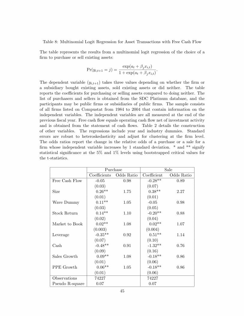
Table 8: Multinomial Logit Regression for Asset Transactions with Free Cash Flow

The table represents the results from a multinomial logit regression of the choice of afirm to purchase or sell existing assets:

Pr(yi,t+1 = j) =exp(at + βjxi,t)

1 + exp(at + βjxi,t).

The dependent variable (yi,t+1) takes three values depending on whether the firm ora subsidiary bought existing assets, sold existing assets or did neither. The tablereports the coefficients for purchasing or selling assets compared to doing neither. Thelist of purchasers and sellers is obtained from the SDC Platinum database, and theparticipants may be public firms or subsidiaries of public firms. The sample consistsof all firms listed on Compustat from 1984 to 2004 that contain information on theindependent variables. The independent variables are all measured at the end of theprevious fiscal year. Free cash flow equals operating cash flow net of investment activityand is obtained from the statement of cash flows. Table 2 details the constructionof other variables. The regressions include year and industry dummies. Standarderrors are robust to heteroskedasticity and adjust for clustering at the firm level.The odds ratios report the change in the relative odds of a purchase or a sale for afirm whose independent variable increases by 1 standard deviation. * and ** signifystatistical significance at the 5% and 1% levels using bootstrapped critical values forthe t-statistics.

Purchase SaleCoefficients Odds Ratio Coefficient Odds Ratio

Free Cash Flow -0.05 0.98 -0.28** 0.89(0.03) (0.07)

Size 0.26** 1.75 0.38** 2.27(0.01) (0.01)

Wave Dummy 0.11** 1.05 -0.05 0.98(0.03) (0.05)

Stock Return 0.14** 1.10 -0.20** 0.88(0.02) (0.04)

Market to Book 0.02** 1.08 0.02** 1.07(0.003) (0.004)

Leverage -0.35** 0.92 0.51** 1.14(0.07) (0.10)

Cash -0.48** 0.91 -1.32** 0.76(0.09) (0.16)

Sales Growth 0.09** 1.08 -0.18** 0.86(0.01) (0.06)

PPE Growth 0.06** 1.05 -0.18** 0.86(0.01) (0.06)

Observations 74227 74227Pseudo R-square 0.07 0.07

45

0

Profitability (z)

Inve

stm

ent (

I)Optimal Investment

zs(K) z

a(K)

M > 0 →N = 0, M > 0 →

N > 0, M = 0 →

← N = 0, M < 0

Figure 1: The figure plots optimal investment as a function of profitability z for a firm of fixedsize K. za(K) denotes the profitability threshold above which the firm buys existing assets fromanother and zs(K) denotes the profitability threshold below which the firm sells assets.

46

1 2 3 4 5 6 7 80

0.1

0.2

0.3

0.4

0.5

0.6

0.7

Size

Pro

fitab

ility

Plot of Firm Action Boundaries

Sell Assets

Acquire Other Assets

AcquireSell

Figure 2: The figure identifies the regions where firms acquire assets from and sell assets to otherfirms. For a given size, firms with profitability above the top line will acquire assets, and firms withprofitability below the bottom line will sell assets. Firms in the interior will invest in new capital.The resale price of capital, p = 0.98.

47