1

Financial Contracting

Itay Goldstein

Wharton School, University of Pennsylvania

2

The Design of Securities

Traditional capital-structure literature studies the tradeoff between

debt and equity.

A much deeper question is about why these securities emerge in the

first place.

The financial contracting literature addresses this question by

developing the optimality of these securities from primitive

assumptions.

3

Costly State Verification

One approach to this question was pioneered by Townsend (1979)

and followed by Gale and Hellwig (1985).

Entrepreneur and investor write a contract by which the investor

provides financing to a project, and the entrepreneur pays back an

amount that depends on the state of the world.

The state of the world, however, is observed only by the

entrepreneur, and the investor can observe it only by incurring a

monitoring cost. Hence, there is costly state verification.

4

A standard debt contract is shown to be optimal (maximize

entrepreneur’s wealth subject to the participation constraint of the

investor) in this environment.

Here,

o The investor receives a fixed amount and does not verify the

state when the return is above a certain threshold.

o The investor receives the full return of the project (lower than

the fixed amount above) and verifies the state when the return is

below the threshold. This can be thought of as bankruptcy.

5

Formal Analysis: Tirole (Ch. 3.7)

Framework

Entrepreneur’s own wealth is given by A, and so to make an

investment I he needs to raise I-A from an investor.

The investment yields a random return R drawn from density

on 0, ∞ . This return is ex-post known to entrepreneur without cost,

and the investor can verify it at cost of K.

According to an arbitrary financing contract:

6

o The investor provides I-A,

o The entrepreneur invests yielding return R and reporting .

o Conditional on , the investor doesn’t audit (to verify the return)

with probability .

o The investor receives payment in case of no auditing and

, in case of auditing.

The entrepreneur’s return in case of no auditing is ,

, and in case of auditing is , , .

7

Truthful Reporting

According to the revelation principle (Myerson (1979)), we can

restrict attention to contracts that provide incentive for the

entrepreneur to report the return truthfully.

o This principle states that under certain conditions (including the

ability to commit to an action based on the report) any outcome

can be replicated by a contract that induces truth telling.

Then, we write the expected payoff of the entrepreneur as:

, 1 ,

8

Optimal Contract

The optimal contract maximizes the entrepreneur’s expected income

subject to the incentive constraint that the entrepreneur reports

truthfully and to the participation constraint of the investor:

max· , ·,· , ·,·

s.t. max , 1 , (IC)

1 (IR)

9

Since IR is binding, we can rewrite the maximization problem as:

max· , ·,· , ·,·

max· , ·,· , ·,·

1

min· , ·,· , ·,·

1

o That is, we wish to minimize the expected audit costs subject to

the constraints.

10

Standard Debt Contract

A standard debt contract looks as follows:

o Debt payment D.

o 1 if .

o 0 if .

o , 0 ; , .

We go on to show that under deterministic audit, that is,

0 1 , the optimal contract is a standard debt contract.

11

Proof

Under the deterministic audit assumption, there are two regions of

returns: the no-audit region and the audit region .

o and 0, ∞ .

First Property: The payoff to the investor is constant in the

no-audit region . We denote this payoff D, implying that

, ∞

o Suppose to the contrary that , and .

12

o Then, the entrepreneur would report when observing .

Because there is no audit he gets to pay less.

o This violates the incentive compatibility condition required for

truthful disclosure.

By the same argument: The payoff to the investor in the

audit region cannot exceed D.

o Otherwise, observing , the report would be .

Economically, no-audit regions are needed to save costs. They can

only be sustained if they induce maximum payoff to investor.

13

Second Property: the no-audit region , ∞ and the audit

region 0, .

Third Property: In the audit region , the payoff to the investor

.

o Take an arbitrary contract (characterized by regions and ),

which satisfies the two constraints IC and IR, and in which these

properties do not hold.

o Compare it with a debt contract (characterized by and )

paying the same D in the no-audit region.

14

o The debt contract yields lower auditing costs since .

o The debt contract offers a higher payoff to the investor:

It pays him more at since the debt contract

pays D and the arbitrary contract pays at most D.

It pays him more at since the debt contract

pays the maximum available amount R.

It pays him the same (D) at .

o The investor gets a strictly positive value with this debt contract:

15

1 0

o Inspecting this expression, we can see that it is negative when

D=0 and is continuous in D.

o Hence, there exists a debt contract with , such that the

investor participation constraint is binding:

1 0

o This contract is better than the original arbitrary contract since:

16

It has lower monitoring costs than debt contract with D

which are lower than in the original arbitrary contract.

It has the investor participation constraint binding.

It satisfies the incentive compatibility constraint.

o Hence, the arbitrary contract is dominated by a debt contract.

Economically, it is optimal to minimize states where auditing cost

is incurred. Paying full amount to investor when auditing happens

helps reduce the amount D paid when auditing does not happen and

thus reduce the probability of auditing.

17

Random Audits

The optimality of the standard debt contract was established under

the assumption that auditing happens with probability 0 or 1.

It turns out that when one allows for randomization in auditing

decisions, the standard debt contract is no longer optimal, and

randomization is expected to happen.

To illustrate this, consider and in the above

problem ( ).

18

Auditing in state is important, since otherwise the entrepreneur

would be better off misrepresenting in state and claiming it is :

But, when randomization is allowed, a probability of auditing

between 0 and 1 at state can be sufficient to deter the entrepreneur

from misrepresentation while saving on auditing costs.

In fact, a probability in state is going to be sufficient:

19

Other Limitations

The model explains the optimality of outside debt and inside equity.

It does not explain why outside equity may be issued.

The model relies strongly on the notion of commitment:

o Investors commit to audit if the firm reports earnings below D.

o But suppose that renegotiation is allowed. Then, if ex post the

entrepreneur reports a state lower than D and offers to pay D-K,

the investor will not audit.

20

o This undermines incentive to report truthfully and changes the

equilibrium.

The interpretation of stealing and auditing has to be thought through.

o An implicit assumption is that the entrepreneur can steal nothing

from the firm before an audit takes place, but can take the

residual income after repayment if an audit did not take place.

o What is the underlying setting? Entrepreneur steals, but cannot

consume for some time? Deriving utility from stolen income

requires the firm not to shut down?

21

Incomplete Contracts: Aghion and Bolton (1992)

Aghion and Bolton use the incomplete-contracts approach

(Grossman and Hart (1986)) to explain financial contracting.

They enrich the original framework by assuming that the

entrepreneur has limited wealth and needs capital from an investor.

Their focus is not on the payoffs that the contract provides, but on

the control structure. Debt is a mechanism for contingent control:

o Depending on the state of the world, control is shifted to the

party whose interests are aligned with efficiency.

22

The Model (Simplified)

A penniless entrepreneur seeks funding K from an investor at t=0.

There are many investors, so all the bargaining power is at the hands

of the entrepreneur:

o The investor should get back at least K (participation constraint).

At t=1, there is a realization of the state of the world , ,

where happens with probability q. This is followed by an action

taken by the control holder (cannot be contracted): , .

23

At t=2, there is realization of the return of the project 0,1 .

o Denote the expected return in state and given action as:

1 , .

The (risk neutral) investor gets utility only from his share of the

return: .

The (risk neutral) entrepreneur also gets a private benefit:

, , .

o Denote the private benefit in state and given action as .

24

Control Allocation and Payments

Focus on three possibilities: Entrepreneur control, Investor control,

Contingent control (depends on ).

Entrepreneur gets private benefits l and investor gets monetary

benefits y. Fixed payment t can be made to meet participation

constraint (only from investor to entrepreneur).

This is a simplification of the model which assumes that is not

verifiable and control depends on a signal s which is correlated with

, and also allows a payment , which helps align incentives.

25

First-Best Actions

The model assumes that the first-best action in is , and the

first-best action in is :

Also, the first best actions are feasible:

1

26

Comonotonic Benefits

Suppose that , (private benefits are comonotonic).

Then, giving control to the entrepreneur can achieve first best:

o The entrepreneur chooses action in and action in .

o The payment t is set to meet the participation constraint of the

investor: 1 .

Similarly, when and (monetary benefits are

comonotonic), giving control to the investor can achieve first best.

27

No Comonotonicity

The interesting case arises when neither the entrepreneur nor the

investor have incentives that are perfectly aligned with efficiency.

Suppose that , , and and :

o Each one wants to do the efficient thing only in one state.

o Real world interpretation: represents expansion; represents

good state. Expansion is efficient only in good state, whereas

entrepreneur always want to expand and investor never wants to.

28

Entrepreneur Control

Entrepreneur wants to choose in .

With ex-post renegotiation first-best can be restored. Yet, this

might deprive the investor of adequate return, so he doesn’t get K.

In detail:

o When is realized, entrepreneur has incentive to renegotiate.

o Assuming entrepreneur has all the bargaining power, he makes a

take-it-or-leave-it offer that keeps the investor indifferent.

29

o That is, he offers to provide the investor the monetary benefit

, in exchange for a payment of .

o This is beneficial for the entrepreneur because

. He captures the total surplus from the efficient action.

Hence, renegotiation guarantees that the efficient action is taken, but

it doesn’t guarantee the investor to get K back, as the investor is

only getting in . Hence, this doesn’t work if:

1 1 .

30

The paper goes on to analyze the possibility of writing a

renegotiation-proof contract.

o Here, the payment to the entrepreneur is made contingent on the

signal (correlated with the state of the world) and on the final

monetary benefit.

o This provides incentive for the entrepreneur to pick the ‘right’

action without leading to renegotiation.

o This, however, is also costly, as the incentives reduce the return

to the investor, leading to a problem as with renegotiation.

31

For illustration, suppose that the contract specifies a payment

, to the entrepreneur, where 0, and the

investor gets the residual return.

Designing a contract that makes the entrepreneur choose in

amounts to setting high enough ( should be 0).

To cause minimum damage to the investor’s participation constraint,

we want:

32

This implies that:

But then the investor’s return is capped at:

1 1

So this arrangement is not feasible when:

1 1 1 .

33

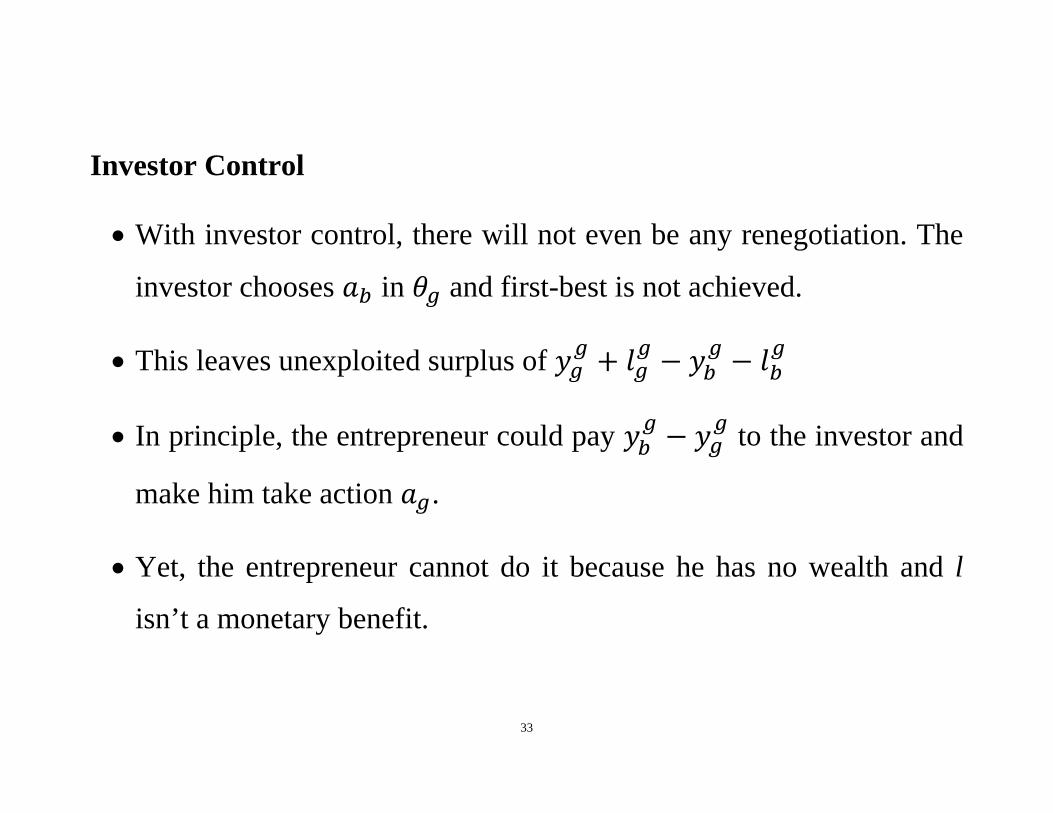
Investor Control

With investor control, there will not even be any renegotiation. The

investor chooses in and first-best is not achieved.

This leaves unexploited surplus of

In principle, the entrepreneur could pay to the investor and

make him take action .

Yet, the entrepreneur cannot do it because he has no wealth and l

isn’t a monetary benefit.

34

Contingent Control

The main point of the paper is that conditioning the control on the

state of the world can achieve first-best when both unilateral control

allocations fail to do so.

Clearly, here, the first-best is achieved if control is given to the

investor in and to the entrepreneur in .

When the state of the world is not verifiable, the allocation can get

very close to first-best if there is a verifiable signal highly correlated

with the state of the world.

35

This allocation of control resembles the allocation under a debt

contract, where creditors get control when the firm is in bad shape.

The underlying intuition is that by giving the investor control in the

bad state, the entrepreneur is able to guarantee him a higher return,

and this relaxes the financing constraint.

One limitation of the model is that it doesn’t have strong predictions

about cash flow rights.

Another limitation is that the event that triggers change in control is

just a bad state, not the default by the firm.

36

The Number of Creditors: Bolton and Scharfstein (1996)

After explaining the emergence of debt contracts, the structure of

debt remains an important question, one aspect of which is the

number of creditors.

Bolton and Scharfstein (1996) develop a theory about the optimal

number of creditors within the incomplete-contracts framework.

The idea is that the number of creditors will affect the bargaining

processes in the event of default. This will affect the liquidation

value of the firm and the likelihood of default, leading to a tradeoff.

37

The Model

A manager with no wealth needs to finance an investment project at

t=0 at a cost of K. This will be spent on two assets A and B.

At t=1, the project generates x with probability or 0 with

probability 1 .

At t=2, if the manager keeps running the project, it yields a cash

flow of y. Alternatively, if the project is liquidated and run by the

investors, it generates 0. If it is liquidated and run by other

managers, it generates ; 1.

38

If it was possible to write a complete contract, it would specify

payments for different cash flows of the firm and ensure that

liquidation doesn’t occur at t=1.

Yet, in the spirit of the incomplete-contracts literature, this is

assumed impossible.

The possibility of liquidation in t=1 is necessary to deter the

manager from diverting cash to himself.

Note that at t=2, there is no way to make the manager pay back to

the investor, as there is no more threat of liquidation.

39

Contract

The most general contract then specifies the probability of

liquidation at t=1 for a payoff R made by the firm to the investors.

(Partial liquidations are shown to be inefficient.)

Hence, if with cash flow x, the manager makes payment ,

investors have the right to liquidate with probability , or .

Similarly, with cash flow 0, we get and .

Of course, payments cannot exceed cash flows: 0 and .

It is straightforward to show that 0 and 0.

40

The goal is to maximize the firm’s expected payoffs:

1 1 .

Denoting the liquidation values as and , the investors’

participation constraint is:

1 0.

The incentive compatibility constraint is:

1

S denotes benefit that the manager has from paying 0 with x cash.

41

We can rewrite the incentive constraint as:

Since both constraints are binding, we plug one in the other:

1 0

Now, we can rewrite the objective function:

1 1

1

1

42

Here, the first three terms capture the expected profit in the first-best

case of no liquidation, and the fourth term captures the loss from

liquidation due to contract incompleteness.

Clearly, the objective function is decreasing in .

Hence, we are going to set at the lowest possible level:

1

There is liquidation in equilibrium in the bad state in order to

incentivize the manager not to divert cash in the good state.

43

Note that the arrangement becomes not feasible if

1 .

o Here, the amount that needs to be financed is too large relative to

the maximum amount that can be promised to the investors.

o Hence, large projects (high ) with low continuation value (low

y), low liquidation value (low ), and high managerial benefit

from liquidation (high S) are less likely to be financed.

o If financed, such projects will exhibit a higher probability of

liquidation.

44

One Creditor

We compute , S, and in case where the firm has one creditor.

:

o Upon liquidity default, the creditor tries to sell the assets to an

outside manager, for whom the continuation value is .

o Suppose that the buyer incurs a cost c to get into bargaining over

the assets, where c is uniformly distributed over 0, .

o The buyer will get into the process if c is less than his payoff.

45

o Assuming Nash bargaining, the surplus will be split between the

creditor and the buyer such that each one of them gets .

o Therefore, the assets are sold with probability .

o Hence, in case of one creditor is:

1 .

S:

o Under strategic default, the manager has cash and so he buys

the firm.

46

o His continuation value is y, so under Nash bargaining both he

and the creditor get:

1 .

:

1

2 1 4

o We can see that the probability of default is decreasing in the

probability of success .

47

Two Creditors

We compute , S, and in case where the firm has two creditors.

The assumption is that each creditor is secured by another asset.

The critical assumption is that the two assets are worth more

together than apart:

∆ 0.

Essentially, there are either increasing returns to scale or

complementarities between the two assets.

48

:

o Now, there are three parties to the bargaining: outside manager

and the two creditors.

o The bargaining outcome is based on the Shapley values.

o Creditor a’s Shapley value is: ∆.

With probability he is in coalition with the other creditor

and the buyer contributing ∆, while with probability

he is in coalition with the buyer contributing .

49

o Creditor b’s Shapley value is: ∆.

o Hence, the Shapley value of the outside manager is ∆.

He is getting less because of the complementarities between

the two creditors. After teaming with one, he needs to pay

more to the other one.

o Based on the logic before, the assets are sold with probability ∆, leading to liquidation value:

2∆ ∆ ∆ .

50

o The liquidation value in case of two creditors is lower than in

case of one borrower.

The creditors squeeze more in case they sell the assets, but

this leads to a lower probability of selling them.

The second effect dominates.

S:

o Based on similar logic:.

2 ∆ .

51

o The manager gets less out of strategic default with two creditors.

The complementarities enable creditors to get a larger share.

:

2

2∆6 1 4

∆36

o Relative to the probability of liquidation with one creditor, there

are two effects: is lower leading to a higher probability of

liquidation, but S is lower leading to a lower probability of

liquidation.

52

Tradeoff

The inefficiency in financing is given by: 1 .

Increasing the number of borrowers has two effects:

o Positive: Making strategic default less tempting, and thus

relaxing the incentive constraint and enabling reduction in .

o Negative: Reducing the liquidation value in case of liquidity

default which affects inefficiency both directly and indirectly via

the increase in the probability of liquidation.

53

Overall, having more creditors increases their bargaining power.

This means they will get less in case of liquidity default (buyers are

less likely to show up), but more in case of strategic default

(manager is already there).

Which effect dominates depends on the parameters.

One can make cross-sectional comparisons:

o Borrowing from one creditor is better when default risk is high

( is low).

54

In this case, the liquidation value upon liquidity default

becomes more important.

o Borrowing from one creditor is better when complementarities

are high (∆ is high).

The effect on the liquidation value is convex.

o Borrowing from one creditor is better when outside managers

are more efficient ( is high).

In this case, the damage to liquidation value becomes more

important.

55

The Diversity of Claims: Dewatripont and Tirole (1994)

Several papers try to explain why a firm has multiple classes of

external securities at the same time.

Dewatripont and Tirole (1994) focus on external equity and debt.

In their model, incentivizing the manager to exert effort requires

commitment to actions that are ex-post not efficient. Since

contracting on such actions is impossible, incentives are given to

different security holders via control and cash flow rights to

implement the optimal plan.

56

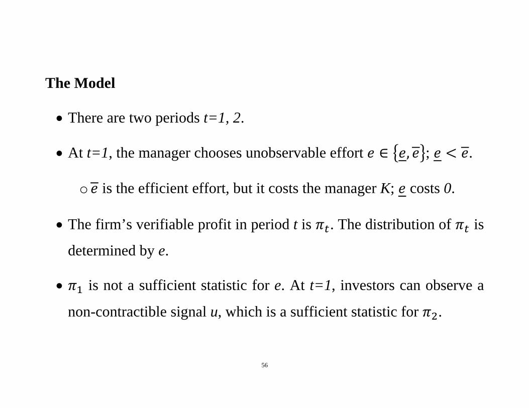
The Model

There are two periods t=1, 2.

At t=1, the manager chooses unobservable effort , ; .

o is the efficient effort, but it costs the manager K; costs 0.

The firm’s verifiable profit in period t is . The distribution of is

determined by e.

is not a sufficient statistic for e. At t=1, investors can observe a

non-contractible signal u, which is a sufficient statistic for .

57

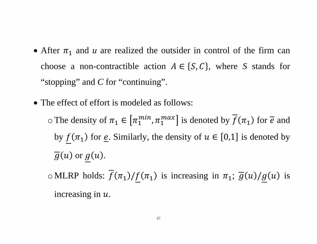
After and u are realized the outsider in control of the firm can

choose a non-contractible action , , where S stands for

“stopping” and C for “continuing”.

The effect of effort is modeled as follows:

o The density of , is denoted by for and

by for . Similarly, the density of 0,1 is denoted by

or .

o MLRP holds: / is increasing in ; / is

increasing in .

58

The effect of the outsider’s action is modeled as follows:

o For each u, the density of , is | for

action C and | for action S. The cumulative functions

are and , respectively.

o Action S is safer than action C: for each u, there exists ,

| |

| |

Hence, equity holders tilt to C and debt holders to S.

59

o Action C becomes more appealing for high signal u:

| | 0 ,

and 0,1 , | |

The manager is assumed to receive private benefit B as long as

outsiders continue the project.

o This is a simple assumption leading to the congruence of

interests between the manager and shareholders.

o The authors show that similar results are obtained with

endogenous monetary benefits.

60

Managerial Incentive Scheme

The program is set to minimize ex-post inefficiency in the choice of

C vs. S subject to the constraint that the manager receives the

incentive to choose .

o The manager’s outside utility is assumed to be 0, and thus the

participation constraint is not binding.

Specifically, we find the optimal probability of continuation

, for each and u.

Since u is non-contractible, we implement it with capital structure.

61

Define the net monetary gain from continuing given signal u:

∆ | |

| | ,

where the second step is obtained after integration by parts.

o ∆ 0, ∆ 0 for , and ∆ 0 for .

Defining ∆ ∆ , 0 and ∆ ∆ , 0 , we

can write the program as:

62

min·,·

1 , ∆ , ∆

Subject to

,

Denote the Lagrange multiplier of this program as . Since ∆

∆ ∆ , we get the derivative of the Lagrangian:

∆

We can see that , is optimally either 0 or 1.

63

Then, since / is increasing in , / is

increasing in , and ∆ is increasing in u, the solution is of the

following form:

, 0 , 1 ,

where is decreasing in .

Intuitively, low u and low lead to action S because they indicate

lack of effort, and thus the manager should be penalized. In addition,

low u makes action S more efficient.

64

65

Outsiders’ Incentive Scheme

Designing outsiders’ incentives via the financial structure of the firm

serves to implement the optimal managerial incentive schemes as

characterized by .

We need at least two outside investors and two classes of securities,

as absent these conditions, continuation will occur if and only if it is

ex-post efficient, i.e., when .

o This implies optimal policy only for profit level , which is

defined by: .

66

o Note that ex-post optimal policy does not depend on , but

such dependence is crucial to implement ex-ante managerial

incentives.

We need to implement a policy that leads to ex-post excessive

continuation when and to ex-post excessive liquidation

when .

The authors show that the optimal plan can be implemented with the

two standard financial instruments: debt and equity.

Suppose that the firm has long-term debt due at t=2 of .

67

Suppose that the investor in control of the decision holds a

proportion of the firm’s debt and a proportion of its equity. For

a given u, a decision to continue yields:

| 1 |

|

While a decision to stop yields:

68

| 1 |

|

After integration by parts, we get the net payoff to continuing:

| |

| |

69

Since continuation becomes more attractive for high u, the investor

in control will continue if and only if u is above some threshold

, , .

Since continuation is riskier, the threshold increases in / :

o For ⁄ 1, the threshold is .

Specializing attention to pure debt or pure equity control, the

optimal plan is to give control to the debt holders when and

to the equity holders when . This is done by setting a short-

term debt level at

70

71

To finalize the implementation of the optimal incentive scheme, we

need to pin down the long-term debt levels .

o These debt levels must vary with first-period profit.

Under equity control ( ), is determined by:

0.

Under debt control ( ), is determined by:

0.

72

We can see that under both debt and equity control, long-term debt

increases in first-period profit .

o In both cases, a higher long-term debt make the decision-maker

consider higher levels of in his decision, which makes

continuation more attractive.

o Interestingly, while higher short-term debt tends to favor

liquidation, higher long-term debt tends to favor continuation.

Yet, there is a jump down in from to as we shift from

the range of debt control to the range of equity control.

73