financial densities in emerging markets

Emerging Markets Review 4(2003) 197–223

1566-0141/03/$ - see front matter� 2003 Elsevier Science B.V. All rights reserved.PII: S1566-0141Ž03.00027-X

Financial densities in emerging markets:an application of the multivariate ES density

Ignacio Mauleon*´

Fac. de Ciencias Jurıdicas y Sociales, Universidad Rey Juan Carlos I, Paseo de los artilleros syn,´Vicalvaro, 28032 Madrid, Spain´

Received 22 November 2001; received in revised form 15 April 2002; accepted 24 May 2002

Abstract

This paper derives and presents the multivariate Edgeworth–Sargan(ES) density, discussessome of its properties, and estimates it for three exchange rates in emerging markets(Chile,Hungary and Singapore). The ES density fits the data adequately, and the model is estimatedsimultaneously for all variables. This involves estimating a highly non-linear model with 32parameters. A multivariate Student’st is also estimated, and both sets of results are compared.The empirical results show that,(a) the ES density applies to emerging markets as well asto more developed economies, as shown in previous research,(b) it is feasible to estimate amultivariate density of large dimensionality, and(c) independent estimation of the marginaldensities, although a consistent procedure, yields significantly different results from themultivariate estimation for some parameters.� 2003 Elsevier Science B.V. All rights reserved.

JEL classifications: C12; G1

Keywords: Multivariate financial densities; Edgeworth expansion; Emerging markets

1. Introduction1

When data are observed at frequencies higher than weekly—and even sometimesmonthly—it is a well-known, and almost universal result, that statistical tests rejectNormality. Departures from Normality have been addressed in applied financial

*Corresponding author. Tel.:q34-91-631-4497; fax: 34-91-631-4498.E-mail address: [email protected](I. Mauleon).´

This research has been conducted under grant SEC98-1112 from the Cicyt. The suggestions of an1

anonymous referee helped improve substantially the paper. The research assistance of Graciela Perez´and Raul Sanchez Larrion is gratefully acknowledged. The author is solely responsible for any possible´ ´´remaining shortcomings.

198 I. Mauleon / Emerging Markets Review 4 (2003) 197–223´

modelling using several different families of probability densities. These includeconvolutions of the Poisson and the Normal(Ball and Roma(1993), Ball andTorous (1983), Akgiray and Booth(1988), Jorion (1988) and Vlaar and Palm(1993)), the logistic(Gray and French(1990) and Aparicio and Estrada(2001)),the exponential power(Gray and French(1990) and Aparicio and Estrada(2001)),non parametric estimation(Silverman (1986), Pagan and Schwertz(1990b) andAıt-Sahalia and Lo(1998)), mixtures of Normals(Hamilton (1991) and Harvey¨and Zhou(1993)), the Gamma(Nelson(1991)), the Generalized Beta(McDonaldand Xu (1995)), the Student’st (Praetz(1972), Blattberg and Gonedes(1974),Rogalski and Vinso(1978) and Zhou(1993)), the GeneralizedT (McDonald andNewey (1988)), the skewedt (Hansen(1994)), the non-centralt (Harvey andSiddique(1999)), and the multivariatet (Prucha and Kelejian(1984)). In particular,this last density has been the subject of much attention, because it can account forthick tails—a well-known feature of financial data—and does not require theexistence of moments of all orders.

A relatively new family of probability densities in applied financial work, is whatwill be called here the Edgeworth–Sargan(ES) probability density function(ESp.d.f. henceforth). This distribution is based on the asymptotic expansions suggestedby Edgeworth and Gram-Charlier, and was first brought into econometrics—althoughat a theoretical level—by Sargan(see, for example, Sargan(1976, 1980)). Severaltheoretical papers on small sample distributions have been based on his work(see,for example, Mauleon(1983), and references therein) and more recently, it has´been applied to investigate the properties of the bootstrap methodology. In thecontext of the present research, the first point to be noticed is that this type ofdensity can account for several departures from normality—in principle an unlimitednumber, and this gives support to a semi non-parametric interpretation; see Gallantand Nychka(1987) and Gallant and Fenton(1996). It can also be shown that,under certain conditions, the ES p.d.f. can approximate any type of density(seeKendall and Stuart(1977), and the references therein). In applied work, the densityhas been recently applied to high frequency data successfully(see, Gallant andTauchen(1989), Bourgoin and Prieul(1997), Mauleon (1997) and Mauleon and´ ´Perote(2000)).

The family of ES p.d.f. has other interesting properties. It is the main purpose ofthis paper to provide a justification for this statement by solving an importantmodelling problem, namely, the fitting of multivariate densities to financial datainvolving several series. This problem can be addressed by means of the multivariateStudent’st p.d.f., as well, and the results of both estimations will be compared.Besides, the paper intends to extend the applicability of the density to a differentkind of framework—financial markets in emerging economies—beyond the morefrequent analysis of developed financial markets(Bekaert et al.(1998), alsounderline the differences in emerging and mature economies of asset markets). Tothat end, the exchange rate vs. the US dollar of three countries from the maineconomically emerging zones have been selected: Singapore for South East Asia,Chile for South America, and Hungary, for the former Eastern block. The adequateempirical performance of the multivariate ES p.d.f. presented in this paper, points

199I. Mauleon / Emerging Markets Review 4 (2003) 197–223´

to the feasibility of estimating higher dimensionality models i.e. with many variables.This is relevant on its own, and in several other fields, such as, for example, theimplementation of risk control techniques like Value at Risk(see, among others,Duffie and Pan(1997), Dowd (1998) and Britten-Jones and Schaefer(1999)).

The paper is organized as follows: Section 2 reviews briefly the univariate ESp.d.f. and some of its properties; Section 3 presents the generalization to themultivariate case, and discusses some empirical problems; Section 4 is devoted tothe empirical results; finally, the fifth and last section summarizes and concludes,while some technical details pertaining to Sections 2 and 3 are left to AppendicesA and B.

2. Univariate ES probability density functions

This section presents a review of the main features of the univariate ES p.d.f.The discussion proceeds by presenting first the univariate density and its basicproperties Eq.(2.1); some potential problems derived from the different estimationmethodologies are then discussed, and the conditional heteroskedasticity model ispresented Eq.(2.2). Multivariate generalizations are introduced in the next sectionbuilding on these results.

The univariate ES p.d.f. of the random variable´ , is given by the followingit

specification,

qS WT Tw z

x |U Xf ´ sa ´ 1q d H ´ , (2.1)Ž . Ž . Ž .is it is s ity ~T T8V Yss1

where a(Ø) stands for aN(0, 1) p.d.f., the d are a set of constants, and theis

polynomialsH (Ø) are defined by the identityD a(´ )s(y1) a(´ )H (´ ). Sinces ss it it s it

the probability integral ofa(´ )H (´ ) is zero (see Appendix B), it follows thatit s it

the probability integral of Eq.(2.1) is 1. It is, also, easily checked that,E(´ )s0it

if d s0 and E(´ )s(1q2d ) (s1, therefore, providedd s0). If d sd s0,2i1 it i2 i2 i1 i2

then the value ofd accounts for asymmetry(d sE(´ )y6), andd for kurtosisi3 i3 it i4

(d s(E(´ )y3)y24) (note, also, that the sum of polynomials can be written as a4i4 it

sum of powers on ; see the Appendix B, Kendall and Stuart(1977) and Mauleonit ´and Perote(2000), for the first eight polynomials and other properties).

This density function has, in principle, several interesting properties, among themost obvious being that:(1) it can be easily generalized to include more parameters,should they be needed,(2) it can account for asymmetries(by means of oddpolynomials), (3) the probability distribution function is easily obtained,(4) it mayallow for conditional heterogeneity(this can be done, by making thed coefficientsis

dependent on past realizations of the random variate; see Gallant and Nychka(1987) on this point; see also Hansen(1994), and Harvey and Siddique(1999) forrelated work). Besides, the analytical tractability of this specification suggests thatit may allow other developments, and one of them, the multivariate extension, isprecisely the topic of the research in this paper(Mauleon (1999), provides a´forecasting stability test under this type of density; see also Mauleon and Perote´


(2000) for an empirical application and comparison to the Student’st). Onespecially useful application may lie in the calculation of VaR. Complex portfoliosfrequently involve positions non-linearly related to underlying assets(i.e. options).One solution to the calculation of VaR in these cases is through simulation(withhistorical or artificially simulated data). But this procedure may be slow and costly,and this has prompted research on analytical approximations(see Britten-Jones andSchaefer(1999) and Duffie and Pan(1997)). The methodology, with some variants,runs as follows: first, approximations based on a quadratic Taylor expansion of theportfolio are derived; secondly, the first two moments of the approximation arecalculated; and thirdly, VaR is calculated with a Gaussian p.d.f. based on the firsttwo moments calculated in the previous step. The ES density provides a moreflexible framework in the last two steps of this procedure(because it depends onmore than two parameters). It also gives more flexibility compared, for example, tothe Student’st, since this last p.d.f. has moments limited by the number of degreesof freedom, while the ES p.d.f. has moments of all orders(in practice, the estimatednumber of degrees of freedom with financial data may be rather low, withoutdelivering a better fit at the tails(see Mauleon and Perote(2000)).´

Before the advent of computers, the ES density was estimated by the method ofmoments. But beyond the variance, efficient moment estimation requires very largesample sizes. Therefore, negative values for the estimated p.d.f. can sometimeshappen. Shenton(1951) and Barton and Dennis(1952) tackled the problem andprovided specific restrictions to ensure positive density values for the casess4 andd sd s0. The restriction was given as a non-linear inequality constraint, defining1 2

a region of admissible values for(d , d ). They also suggested a generalization for3 4

s)4 that leads to an inequality constraint, highly non-linear in this case. However,in the context of maximum likelihood estimation, and within a given available dataset, this problem cannot occur: this is because a value of the density approachingzero, implies that the value of the log likelihood would approachy`, andmaximum likelihood estimation implies that the chosen set of parameter estimates,yields the maximum possible value for the log of the likelihood(notice that thisresembles the maximum likelihood estimation of the variance: it always yields apositive value, without any need to impose specifically the restriction).

In some instances, the maximum likelihood approach may not be suitable, though.The methodology of Barton and Dennis, would then be a possible solution. Anotherapproach is suggested by Gallant and Nychka(1987). They start by writing thesum of polynomials in Eq.(2.1) as a sum of powers on , and then proceed toit

square it so as to achieve non negativity. A non-linear equality restriction on thepolynomial coefficients is then imposed, to ensure that the probability integral isone. This idea is pursued here, but with some modifications that allow an easiergeneralization to the multivariate context(see Appendix A). It is shown that theparameters of the density of Eq.(2.1) can be made to depend on a reduced set of(unrestricted) coefficients, a property that makes this approach very convenient forapplied work(see, again, Appendix A).

A generalization to allow for an arbitrary, and time varying variance, is easilyobtained through a standard scale transformation,u ss ´ , the density ofu , beingit it it it


given now by f(u ys )ys . The type of model to deal with conditional heteroske-it it it

dasticity implemented in the empirical applications of this paper belongs to thegeneral class of Garch(p, q) models(see Bollerslev et al.(1994) for a review). Fora Garch(1,1), which is the model that fits the data adequately, and in order tospecify fully the notation, the model is the following,

2 2 2s sa qa s qa u , (2.2)it i0 i1 ty1 i2 ty1

where (a , a , a ))0. Goodhart and O’Hara (1997), cast some doubt on thei0 i1 i2

economics of this model, but in practice it works well; see also Mauleon(1997).´The conditional variance for the density of Eq.(2.1), v , will be given by (1q2

it

2d )s . Therefore, the unconditional variance,v , will be (1q2d )s . It is easily2 2 2i2 it i i2 i

checked now that,

2v sg a y 1yg a ya (2.3)Ž .i i i0 i i2 i1

where g s(1q2d ). The denominator(1yg a ya ) is of special interest,i i2 i i2 i1

inasmuch as it measures the degree of near non stationarity of the unconditionalvariance—in the sense that there is no stable distribution ast™`, when (1yg a ya )-0; if it equals zero the distribution exists, although the variance clearly,i i2 i1

does not; see Lamoureux et al.(1990), Pagan and Schwertz(1990a), Phillips andLoretan(1994) and Phillips(1995) for further discussion whend s0.i2

3. Multivariate probability density functions

This section analyses the multivariate densities implemented in the empiricalsection, and some specific empirical problems. Section 3.1 discusses the generali-zation of the univariate ES density given in the previous section to the multivariatecase; three particular cases of special interest are highlighted. Section 3.2 reviewsthe multivariatet density, and Section 3.3 briefly covers some specific empiricalquestions.

3.1. Multivariate ES densities

Fisrt, a general bivariate ES p.d.f. is derived from univariate results Eq.(3.2);correlation among variates is then introduced in a simple way Eq.(3.3); twosimplified versions useful in applied work are then discussed Eqs.(3.6) and (3.9),and generalized to then-variate case Eqs.(3.8) and(3.10); the ability of the ES todeal with other crossed relationships among variates beyond correlation, such as co-skewness and co-kurtosis, in a simple way is also shown Eq.(3.7); finally, arestricted version devised to avoid negative values where they might appear is alsopresented Eq.(3.11) (the more technical details are left to the Appendix A).

We start by defining the bivariate ES density by a straightforward multiplication


of two independent ES densities, given in Eq.(2.1), and rearrange the result asgiven next:

q qw z w zS WS WT TT T

U XU Xf ´ ,´ s a ´ 1q d H ´ a ´ 1q d H ´Ž . Ž . Ž . Ž . Ž .x | x |1t 2t 1t 1s s 1t 2t 2s s 2tT TT T8 8V YV Yy ~ y ~ss1 ss1

q q qw zST

Usa ´ a ´ 1q d H ´ q d H ´ q d H ´Ž . Ž . Ž . Ž . Ž .x |1t 2t 1s s 1t 2s s 2t 1s s 1tT 8 8 8V y ~ss1 ss1 ss1

Wqw zTX= d H ´Ž .x |2s s 2t8 T

y ~Yss1

q qST

Usa ´ a ´ 1q d H ´ q d H ´Ž . Ž . Ž . Ž .1t 2t 1s s 1t 2s s 2tT 8 8V ss1 ss1

Wq qw zTXq d d H ´ H ´ . (3.1)Ž . Ž .x |1s 2r s 1t r 2t88 T

y ~Yss1rs1

The last term involving the product of polynomials embodies a set of restrictionson the coefficients, that can be relaxed introducing a new set of parametersg (sssr

2,«, q, rs2,«, q), where, in general,g /d d . The previous bivariate densitysr 1s 2r

can be written, now, as follows,

f ´ ,´ sa ´ a ´Ž . Ž . Ž .1t 2t 1t 2t

Wq q q qw zSTT

U X= 1q d H ´ q d H ´ q g H ´ H ´ , (3.2)Ž . Ž . Ž . Ž .x |1s s 1t 2s s 2t sr s 1t r 2tT 8 8 88 TV y ~Yss1 ss1 ss1rs1

and this provides a completely general bivariate ES density. Notice that the numberof parameters has increased considerably, and is equal toq q2q (qs8, a typical2

value in applied work, yields 80 parameters, just for the bivariate case, and withoutaccounting for correlation, yet). Notice, also, that the two variates(´ , ´ ), are1t 2t

still uncorrelated, but not independently distributed anymore.Replacing the leading terma(´ )a(´ ) by a bivariate Gaussian density with1t 2t

covariance matrixR, denoted byb(Ø), yields, finally,

f ´ , ´ sb ´ , ´ qa ´ a ´Ž . Ž . Ž . Ž .1t 2t 1t 2t 1t 2t

Wq q q qw zSTT

U X= d H ´ q d H ´ q g H ´ H ´ , (3.3)Ž . Ž . Ž . Ž .x |1s s 1t 2s s 2t sr s 1t r 2tT8 8 88 TV y ~Yss1 ss1 ss1rs1

(notice that if the marginals p.d.f. are centered,d sd s0; similarly, we impose11 21

g s0). It is easily checked, now, that the probability integral is one, as required11

for a well-defined p.d.f.(see comment below Eq.(2.1), and the properties in


Appendix B). It is worth noticing, as well, that the covariance matrix is(´ 9s(´ ,t 1t

´ )),2t

E ´ ´9 sR, (3.4)Ž .t t

where, in order to achieve scale normalization, and without loss of generality,R sii

1. The marginal densities are as given in Eq.(2.1), because, 1) the marginal densityof b(´ , ´ ) yields aN(0, 1), given the normalization ofR, and, 2) the integral of1t 2t

the Hermite polynomials times aN(0, 1) p.d.f. in the space(y`, q`) vanish(see, again Appendix B).

The two properties of the multivariate ES density Eq.(3.3) just discussed arespecially convenient in its empirical implementation, since they jointly providereasonable starting values for an otherwise highly non-linear algorithm. In particular,they provide a straightforward methodology to estimate the joint density buildingon univariate estimation results, since the relationship between the univariate andmultivariate parameters is direct: the sample correlation provides a consistentestimate of the true correlation, and the univariate parameters of the Hermiteexpansion i.e. thed ’s—are precisely the same in the univariate and multivariateis

densities. This allows estimating the joint density starting from the univariate results,thus avoiding the problem of estimating a highly non-linear model with manyparameters, without a clear starting point for the optimization algorithm.

The generalization to ann-variate context, and several special cases are analysedin what follows. Before proceeding further, a brief discussion on alternative waysto derive a general multivariate ES p.d.f. may be in order, though. The first andstraightforward suggestion, is simply to consider a non singular linear transformationof a vector of jointly distributed ES random variates(i.e. a linear transformation ofthe vector(´ , ´ ) that follows the general ES distribution given in Eq.(3.2)).1t 2t

While this procedure would certainly induce correlation among both variates, thefinal parameters would be more difficult to interpret and relate to the originalunivariate densities, than as given in Eq.(3.3), without providing any apparentadvantage. Another proposal would simply be the straightforward generalization ofthe univariate density, i.e. an expansion of the multivariate Gaussian density interms of its derivatives. Although this form may be useful for some theoreticalpurposes, it is rather difficult to handle in practice and, again, does not provide anyspecially useful insight. Therefore, the remainder of discussion will build on theform given in Eq.(3.3).

3.1.1. ES type IThe first specific multivariate ES density(ES Type I in what follows) proposed

in this paper, is based on the simplification induced by the restrictiong sd d ,sr 1s 2r

in the density of Eq.(3.3). This allows a significant reduction in the number of


parameters, which may be useful in applied work(at least in a first step). Morespecifically, the bivariate density will now be given as follows,

f ´ ,´ sb ´ ,´ qa ´ a ´Ž . Ž . Ž . Ž .1t 2t 1t 2t 1t 2t

Wq q q qw zSTT

U X= d H ´ q d H ´ q d d H ´ H ´ . (3.5)Ž . Ž . Ž . Ž .x |1s s 1t 2s s 2t 1s 2r s 1t r 2tT8 8 88 TV y ~Yss1 ss1 ss1rs1

In order to generalize it to then-variate case, this expression can be rewritten ina straightforward way as follows,

q qST

Uf ´ ,´ sb ´ ,´ qa ´ a ´ 1q d H ´ q d H ´Ž . Ž . Ž . Ž . Ž . Ž .1t 2t 1t 2t 1t 2t 1s s 1t 2s s 2tT 8 8V ss1 ss1

Wq qw zTXq d d H ´ H ´ y1Ž . Ž .x |1s 2r s 1t r 2t88 T

y ~ Yss1rs1

sb ´ ,´Ž .1t 2t

S Wq qw zw zT TU Xqa ´ a ´ 1q d H ´ 1q d H ´ y1 . (3.6)Ž . Ž . Ž . Ž .x |x |1t 2t 1s s 1t 2s s 2t8 8T T

y ~y ~V Yss1 ss1

If required, the hypothesisg sd d can be tested easily by adding the termsr 1s 2r

(w H (´ )H (´ )), wherew s(g yd d ), to the term inside{ Ø} , and testingsr s 2t r 1t sr sr 1s 2r

w s0. As a case of special interest, consider testing for coskewness as defined bysr

Harvey and Siddique(2000). Assuming both marginal p.d.f. to be centeredd s11

d s0, so thatw sg , and for the p.d.f. of Eq.(3.3) it can be checked after21 12 12

straightforward calculations thatE(´ ´ )s2g . Coskewness can be immediately21t 2t 12

tested by adding the term,

2g x x y1 , (3.7)Ž .12 1 2

and testing the nullg s0. Cokurtosis, as defined by Ang et al.(2002), can be12

tested similarly. First, it can be shown thatE(´ ´ )s3g q6g , so that the term31t 2t 11 13

to add would be(g x x qg x H (x )). Finally, the null would beg q2g s0.11 1 2 13 1 3 2 11 13

Testing this hypothesis simplifies slightly if we assumeg s0, a natural assumption11

to make(see below Section 3.3).The generalization of the bivariate density of Eq.(3.6) to the n-variate case is

immediate, leading to,

n n qw z w zS WT T

U Xf ´ sb ´ q a ´ 1q d H ´ y1 , (3.8)Ž . Ž . Ž . Ž .x | x |t t it is s itT T2 2 8V Yy ~ y ~is1 is1 ss1

where´ s(´ ,«, ´ ).t 1t nt


3.1.2. ES type IIA further simplification can be introduced by deleting the non-linear cross-product

term in Eq.(3.6) altogether(ES Type II henceforth; see also Perote(1999)). Thus,we get,

q qS WT T

U Xf ´ ,´ sb ´ ,´ qa ´ a ´ d H ´ q d H ´ . (3.9)Ž . Ž . Ž . Ž . Ž . Ž .1t 2t 1t 2t 1t 2t 1s s 1t 2s s 2tT T8 8V Yss1 ss1

The marginal densities are still of the form Eq.(2.1), but the variates are notindependently distributed anymore, even in the case of null correlation(preciselybecause deleting the cross product term prevents writing the density as the productof the two independent densities). For the generaln-variate case this simplificationyields,

n n qw z w zS WT T

U Xf ´ sb ´ q a ´ d H ´ . (3.10)Ž . Ž . Ž . Ž .x | x |t t it is s itT T2 8 8V Yy ~ y ~is1 is1 ss1

3.1.3. ES type IIIThe last type of multivariate ES density suggested here(ES Type III henceforth),

embodies the restrictions that ensuref(´ )00 for every possible set of parametert

values. The specific form may look rather arbitrary at first sight. However, it isderived following the same guidelines that allow deriving a general ES used beforein Eqs. (3.6) and (3.9), although starting from univariate restricted ES densitiesthat ensure non negativity(see Appendix A for a detailed derivation). The specificform of the p.d.f. for ann dimensional vector is given as follows,

n n mw zw zS WT T

U Xf ´ sWb ´ q a ´ v q c H ´ yW , (3.11)Ž . Ž . Ž . Ž .x |x |t t it i is s itT T2 2 8V Yy ~y ~is1 is1 ss0

where andv are specific constants for every marginal p.d.f.(see,nWs v ,i i2is1

again Appendix A for details; the remaining symbols are defined as before). Themarginal densities take the general form of the univariate ES(see Eq.(2.1)), butwith restricted parameters ensuring non negativity. These restrictions imply thatmmust be even, and thec depend onmy2 unrestricted parameters for every marginalis

p.d.f. (the details are fully laid out in Appendix A). If m is equal toq in the EStypes I and II given in Eqs.(3.6) and (3.9), that implies that this form of themultivariate p.d.f. is more restrictive; to take the other extreme, ifm is equal to 2q,then it is not. Nonetheless, in this last case the polynomials defining the marginalp.d.f.’s are far more non-linear, raising the possibility of less smooth density shapes(multimodalities, for example), which may or may not be a suitable empiricalproperty. Finally, the covariance matrix is given by (WR), so that,

E ´ ´ sWR (3.12)Ž .it jt ij


3.2. The multivariate t density

The multivariatet p.d.f. is given by,

B Enqnny2 C Fn G

D G2y nqn y2y1y1y2 ( )Z Zf ´ s S nq´9S ´ , n)0, (3.13)Ž . Ž .t t tB Enny2 C Fp G

D G2

where´ is an n dimensional vector, andn is the degrees of freedom(note that itt

does not have necessarily to be an integer). The marginal densities aret densitiesof n degrees of freedom themselves. Similarly to the univariatet, it can be shownthat if y is a random vector distributed as a multivariateN(0, S), andu a randomscalar distributed as ax independently ofy, thenyy6(uyn) follows the multivariate2

n

t p.d.f. as given in Eq.(3.13) (see, for example, Anderson(1984)). It is a symmetricdensity, so thatE(´ )s0. If n)2 the covariance matrix is given byV(u)s(ny(nyt

2))S, whereS is a non singular squared symmetric matrix or ordern (if n(2 itdoes not exist). It is immediate that a non singular linear transformation yields,again, a multivariatet p.d.f., with an equal number of degrees of freedom. Thetransformation that yields uncorrelated variables, however, does not lead to theproduct of independent densities: therefore, uncorrelation does not imply independ-ence in this case. It is also easily checked, that the product of independentt densitiesdoes not yield the multivariatet, as defined in Eq.(3.13). The conditional densityobtained from Eq.(3.13), is itself at p.d.f. (see, for example, Leamer(1978)), andthe sum of two independentt densities does not follow at density(i.e. it does notreproduce through the sum, contrary to the Gaussian andx densities; see, for2

example, Kendall and Stuart(1977)). Other properties and descriptions can befound in Leamer(1978) and Bernardo and Smith(1994).

The univariatet p.d.f. has been extensively used in applied finance to model tailthickness of high frequency financial data, and it has also been extended to allowfor skewness(see the references in Section 1). Similarly, the multivariatet p.d.f.,has been implemented to deal with fat tails and outliers, when modelling empiricalfinancial densities(an early reference in this sense is Prucha and Kelejian(1984),who extended the methodology of simultaneous equation estimators with Gaussianerrors, to the case of multivariatet distributed errors).

3.3. Further empirical problems

There remain two further points to be discussed. The first is conditionalheteroskedasticity, always relevant when dealing with financial data. In the presentcontext this is compounded by the multivariate framework. The second derives fromthe different sample sizes available for the several variables. The first is dealt within the empirical section with the Bollerslev(1990) model, briefly reviewed below.Let us define now, the diagonal matrixL , with s in its ith diagonal position,st it


s being the conditional variance of theith variate as given in Eq.(2.2), and the2it

linear transformation defining the vectoru as follows,t

u sL ´ . (3.14)t s tt

The joint density of the vectoru , is immediately obtained in the usual way. Thet

density f(´ ) can adopt one of the forms given previously in Eqs.(3.6), (3.10),t

(3.11) and (3.13), and the final density for the vectoru is, thus, completelyt

specified. The covariance matrixV of the vectoru , is given now by,t t

V sE u u9 sL E ´ ´9 L . (3.15)Ž . Ž .t t t s t t st t

where(E(´ ´ 9), is given in Eqs.(3.4), (3.12) and (3.13) depending on the chosent t

density). In this way,V , besides being time dependent, it will always be positivet

definite, as required for a covariance matrix. There is empirical evidence thatcorrelations may be time dependent(see Erb et al.(1994) and Longin and Solnik(2001)), and this could be taken into account in the previous model. But, as notedin Bekaert et al.(1998), this feature is less prominent in emerging markets(thispoint is also confirmed by the empirical results of the next section). This is not themain focus of the present paper, however, and remains for future research.

Another empirical problem derives from the different sample sizes available forthe several variables. A straightforward approach would just drop the non commonsample observations, establishing thus, a unified sample. But this implies, no doubt,losing useful information, especially when the amount of observations dropped issignificant. This problem was encountered with the available sample, and thefollowing solution was implemented,

†f ´ s 1yd f ´ qd f ´ , (3.16)Ž . Ž . Ž . Ž .t m 1t m t

where f(´ ) is any of the densities discussed previously in this section,f(´ ) is thet 1t

corresponding marginal density of , and d is a dummy variable containing1t m

zeroes for the first part of the sample, when only observations for´ are available,1t

and ones thereafter, when all variables are observed. The suggested solution,therefore, is a straightforward way to deal with the missing observations in thecontext of maximum likelihood estimation. Notice, finally, that the problem justdiscussed is likely to be encountered when dealing with emerging markets, sincedata sets tend to be gathered in a more irregular fashion.

4. Empirical results

This section presents and discusses the empirical results obtained estimating themodels introduced in Section 3. Some general questions, such as the data base, theOls models fitted to the raw data, and the required notation are commented first.An assessment with comparisons of all the estimated results(given in Tables 1–6)follows; finally, a summary of the main results is provided.


Table 1Univariate ES

Ch Hg Sg

a0 0.000169 0.000757 y0.0000574(1.6) (4.1) (1.1)

a1 0.0415 y0.202 y0.117(1.1) (5.7) (7.9)

a2 0.04800 0.0911 n.s.(2.5) (2.8)

a0 0.00000041 0.00000066 0.00000028(2.7) (1.0) (14.5)

a1 0.822 0.921 0.853(18.8) (15.9) (169.7)

a2 0.244 0.0174 0.161(4.2) (2.3) (19.9)

d2 y0.18 0.453 y0.0644(6.6) (6.1) (4.0)

d4 0.0977 0.179 0.117(3.8) (4.1) (9.99)

d6 0.0127 0.032 0.0170(2.0) (2.7) (5.2)

d8 0.00243 0.0039 0.0028(4.0) (3.7) (9.7)

Correlation matrixCh 1.0 0.121 0.155

(3.1) (4.0)

Hg 1.0 0.213(5.5)

Sg 1.0

Since the purpose of this research was to study the properties of some financialseries in emerging markets, three representative countries have been chosen fromthe main world emerging economic areas: Chile, for South America, Singapore, forSouth East Asia, and Hungary, for the former Eastern block. The series analysed inall cases are the exchange rate with respect to the US dollar. The data have beentaken from the base kept by W. Antweiler, from the University of British Columbiain the internet. Observations are daily, and cover the period(16y11y1995–29y1y1999, 768 observations) for Hungary and Chile, and(2y1y1981–31y12y1998, 4056observations) for Singapore. Since the sample size differs, and in order to maximizethe sample information, the procedure described in Eq.(3.16) in the previoussection has been implemented.

In order to conduct the empirical analysis, first, one logarithmic difference wasapplied to the data. Secondly, and since the purpose was to estimate a simultaneous


Table 2Multivariate ES type I

Ch Hg Sg

a0 0.0000993 0.000512 y0.0000340(1.5) (3.6) (1.1)

a1 y0.000308 y0.130 y0.080(0.73) (4.2) (5.0)

a2 0.0159 0.0868 n.s.(1.2) (2.3)

a0 0.00000045 0.00000113 0.000000297(2.6) (1.0) (5.4)

a1 0.812 0.883 0.849(16.4) (9.4) (50.3)

a2 0.261 0.020 0.16(3.8) (2.3) (6.7)

d2 y0.186 0.448 y0.0556(7.1) (6.0) (2.4)

d4 0.099 0.180 0.122(3.9) (4.1) (10.0)

d6 0.012 0.033 0.0185(1.8) (2.8) (5.4)

d8 0.00245 0.0043 0.00294(3.6) (3.9) (9.7)


(0.79) (1.93)

Hg 1.0 0.0783(2.1)

Sg 1.0

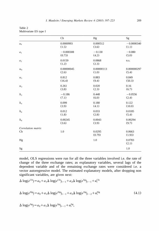
model, OLS regressions were run for all the three variables involved i.e. the rate ofchange of the three exchange rates; as explanatory variables, several lags of thedependent variable and of the remaining exchange rates were considered i.e. avector autoregressive model. The estimated explanatory models, after dropping nonsignificant variables, are given next:

Ch Ch Sg ChD log e sa qa D log e qa D log e quŽ . Ž . Ž .ty1 ty10 1 2 t

Hg Hg Sg HgD log e sa qa D log e qa D log e qu (4.1)Ž . Ž . Ž .ty1 ty20 1 2 t

Sg Sg SgD log e sa qa D log e qu ,Ž . Ž .ty10 1 t


Table 3Multivariate ES type II

Ch Hg Sg

a0 0.000177 0.000715 y0.00003(2.7) (5.0) (1.0)

a1 0.130 y0.173 y0.094(3.4) (5.4) (6.0)

a2 0.0191 0.0570 n.s.(1.6) (2.0)

a0 0.00000019 0.0000031 0.00000025(3.0) (1.7) (5.5)

a1 0.845 0.739 0.861(44.3) (5.9) (62.1)

a2 0.41 0.0582 0.145(6.5) (2.7) (8.3)

d2 y0.28 0.206 y0.0467(13.2) (3.3) (2.2)

d4 0.0777 0.118 0.121(4.5) (2.8) (10.0)

d6 0.0005 0.0259 0.0188(0.11) (2.3) (5.5)

d8 0.00154 0.00359 0.00294(2.9) (3.3) (9.6)


(1.1) (3.5)

Hg 1.0 0.09(2.5)

Sg 1.0

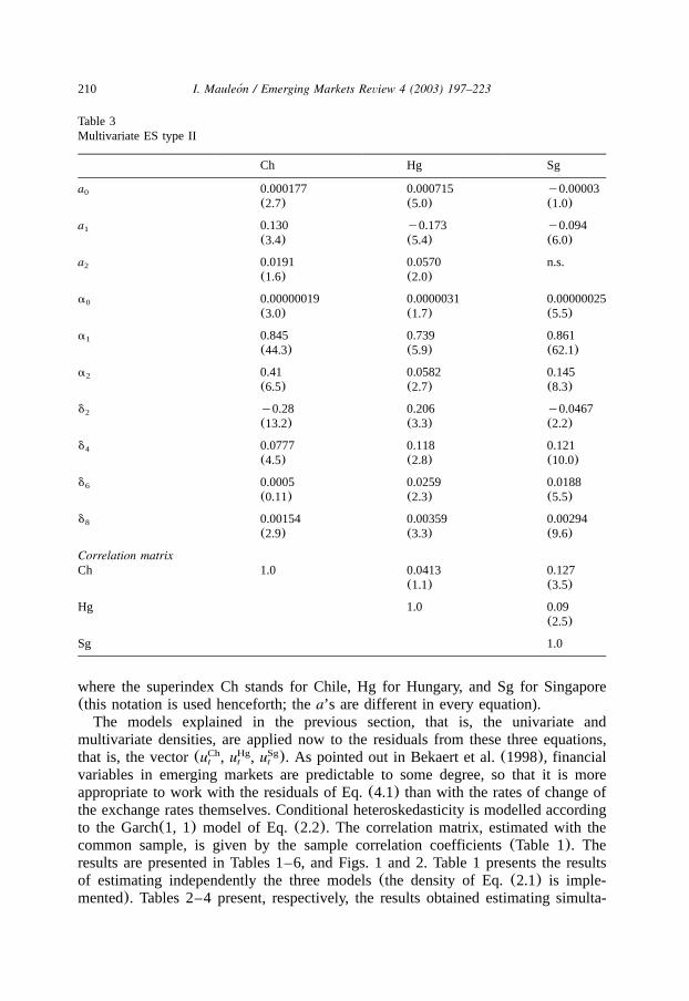
where the superindex Ch stands for Chile, Hg for Hungary, and Sg for Singapore(this notation is used henceforth; thea’s are different in every equation).

The models explained in the previous section, that is, the univariate andmultivariate densities, are applied now to the residuals from these three equations,that is, the vector(u , u , u ). As pointed out in Bekaert et al.(1998), financialCh Hg Sg

t t t

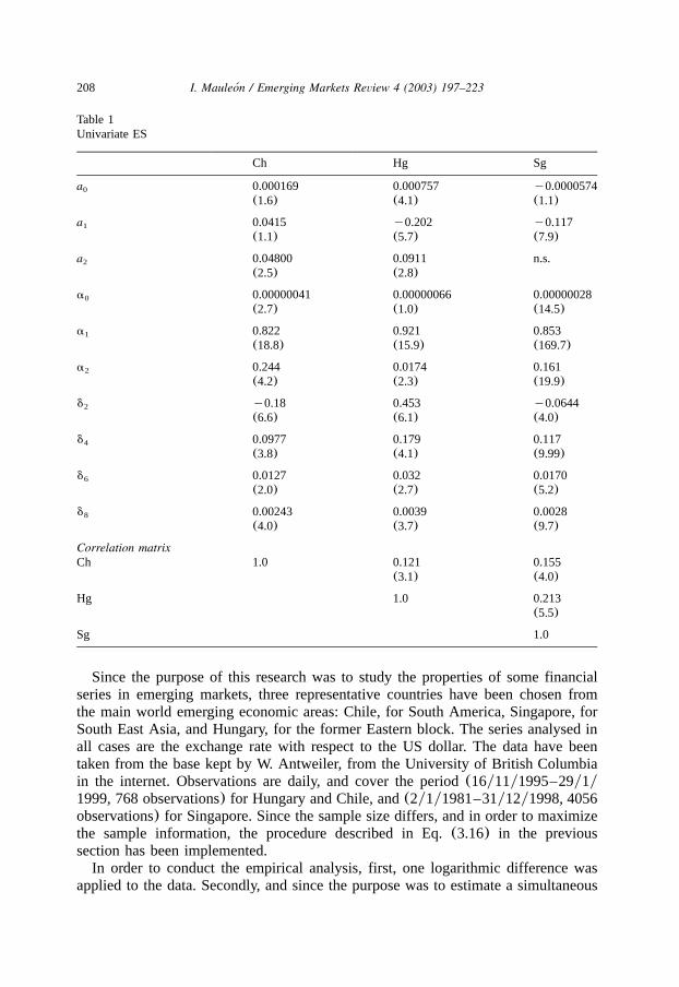
variables in emerging markets are predictable to some degree, so that it is moreappropriate to work with the residuals of Eq.(4.1) than with the rates of change ofthe exchange rates themselves. Conditional heteroskedasticity is modelled accordingto the Garch(1, 1) model of Eq.(2.2). The correlation matrix, estimated with thecommon sample, is given by the sample correlation coefficients(Table 1). Theresults are presented in Tables 1–6, and Figs. 1 and 2. Table 1 presents the resultsof estimating independently the three models(the density of Eq.(2.1) is imple-mented). Tables 2–4 present, respectively, the results obtained estimating simulta-


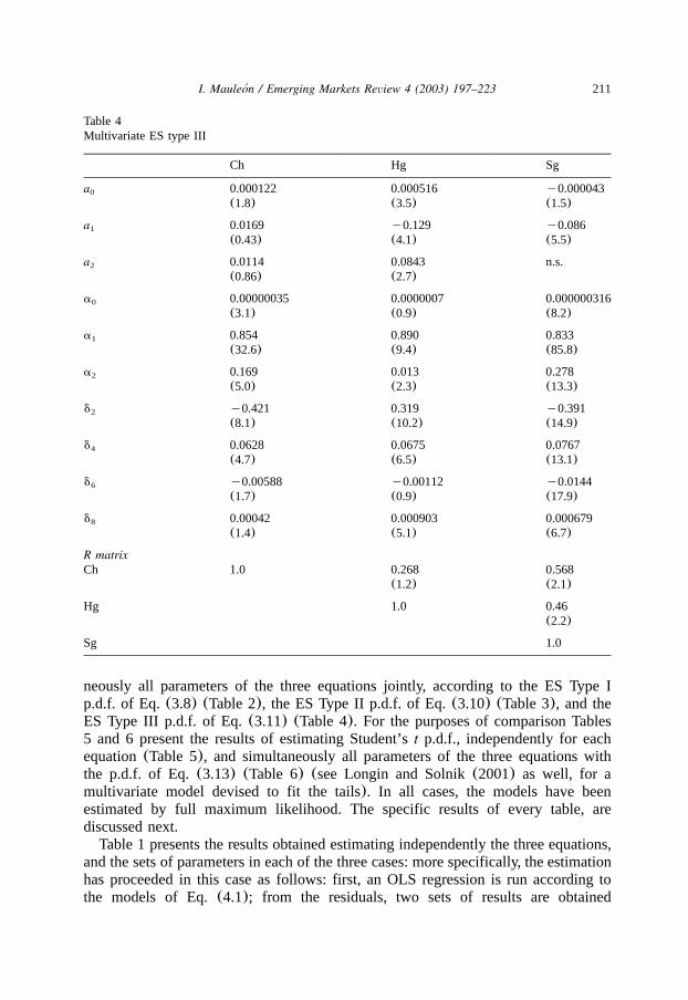
Table 4Multivariate ES type III

Ch Hg Sg

a0 0.000122 0.000516 y0.000043(1.8) (3.5) (1.5)

a1 0.0169 y0.129 y0.086(0.43) (4.1) (5.5)

a2 0.0114 0.0843 n.s.(0.86) (2.7)

a0 0.00000035 0.0000007 0.000000316(3.1) (0.9) (8.2)

a1 0.854 0.890 0.833(32.6) (9.4) (85.8)

a2 0.169 0.013 0.278(5.0) (2.3) (13.3)

d2 y0.421 0.319 y0.391(8.1) (10.2) (14.9)

d4 0.0628 0.0675 0.0767(4.7) (6.5) (13.1)

d6 y0.00588 y0.00112 y0.0144(1.7) (0.9) (17.9)

d8 0.00042 0.000903 0.000679(1.4) (5.1) (6.7)

R matrixCh 1.0 0.268 0.568

(1.2) (2.1)

Hg 1.0 0.46(2.2)

Sg 1.0

neously all parameters of the three equations jointly, according to the ES Type Ip.d.f. of Eq.(3.8) (Table 2), the ES Type II p.d.f. of Eq.(3.10) (Table 3), and theES Type III p.d.f. of Eq.(3.11) (Table 4). For the purposes of comparison Tables5 and 6 present the results of estimating Student’st p.d.f., independently for eachequation(Table 5), and simultaneously all parameters of the three equations withthe p.d.f. of Eq.(3.13) (Table 6) (see Longin and Solnik(2001) as well, for amultivariate model devised to fit the tails). In all cases, the models have beenestimated by full maximum likelihood. The specific results of every table, arediscussed next.

Table 1 presents the results obtained estimating independently the three equations,and the sets of parameters in each of the three cases: more specifically, the estimationhas proceeded in this case as follows: first, an OLS regression is run according tothe models of Eq.(4.1); from the residuals, two sets of results are obtained


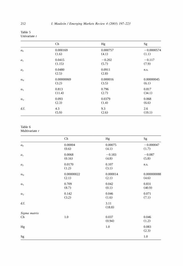
Table 5Univariatet

Ch Hg Sg

a0 0.000169 0.000757 y0.0000574(1.6) (4.1) (1.1)

a1 0.0415 y0.202 y0.117(1.15) (5.7) (7.9)

a2 0.0480 0.0911 n.s.(2.5) (2.8)

a0 0.00000069 0.000016 0.00000045(3.2) (3.5) (6.1)

a1 0.813 0.796 0.817(11.4) (2.7) (34.1)

a2 0.093 0.0379 0.068(2.3) (1.4) (6.6)

d.f. 4.3 9.3 2.6(5.9) (2.6) (19.1)

Table 6Multivariate t

Ch Hg Sg

a0 0.00004 0.00075 y0.000047(0.6) (4.1) (1.7)

a1 0.0068 y0.183 y0.087(0.16) (4.8) (5.8)

a2 0.0170 0.107 n.s.(1.2) (3.1)

a0 0.00000022 0.000014 0.000000088(2.1) (2.1) (4.6)

a1 0.709 0.042 0.831(8.7) (0.1) (40.9)

a2 0.142 0.046 0.071(3.2) (1.6) (7.1)

d.f. 3.11(18.8)

Sigma matrixCh 1.0 0.037 0.046

(0.94) (1.2)

Hg 1.0 0.083(2.3)

Sg 1.0


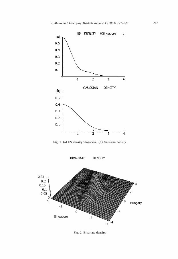
Fig. 1. (a) ES density Singapore;(b) Gaussian density.

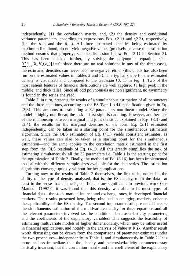
Fig. 2. Bivariate density.


independently,(1) the correlation matrix, and,(2) the density and conditionalvariance parameters, according to expressions Eqs.(2.1) and (2.2), respectively,(i.e. the a ’s and the d ’s). All three estimated densities being estimated byi s

maximum likelihood, do not yield negative values (precisely because this estimationmethod ensures that property; see the discussion below Eq.(2.1) in Section 2).This has been checked further, by solving the polynomial equation,{ 1q

since there are no real solutions in any of the three cases,8 w x}d H (´ ) s0:is s it8ss2

the estimated densities can never become negative, either(this check has also beenrun on the estimated values in Tables 2 and 3). The typical shape for the estimateddensity is visualized and compared to the Gaussian(0, 1) in Fig. 1. Two of themost salient features of financial distributions are well captured(a high peak in themiddle, and thick tails). Since all odd polynomials are non significant, no asymmetryis found in the series analysed.

Table 2, in turn, presents the results of a simultaneous estimation of all parametersand the three equations, according to the ES Type I p.d.f. specification given in Eq.(3.8). This amounts to estimating a 32 parameters non-linear model. Since themodel is highly non-linear, the task at first sight is daunting. However, and becauseof the relationship between marginal and joint densities explained in Eqs.(3.3) and(3.4), the results for the marginal densities of the form Eq.(2.1) estimatedindependently, can be taken as a starting point for the simultaneous estimationalgorithm. Since the OLS estimation of Eq.(4.1) yields consistent estimates, aswell, these values can also be taken as a starting point for the simultaneousestimation—and the same applies to the correlation matrix estimated in the firststep from the OLS residuals of Eq.(4.1). All this greatly simplifies the task ofestimating simultaneously all the 32 parameters i.e. Table 1 is the starting point forthe optimization of Table 2. Finally, the method of Eq.(3.16) has been implementedto deal with the different sample sizes available for the data series. The estimationalgorithms converge quickly without further complications.

Turning now to the results of Table 2 themselves, the first to be noticed is theability of the type of density analysed, that is, the ES density, to fit the data—atleast in the sense that all thed coefficients are significant. In previous work(sees

Mauleon (1997)), it was found that this density was able to fit most types of´financial data—the stock market, interest and exchange rates, in developed financialmarkets. The results presented here, being obtained in emerging markets, enhancethe applicability of the ES density. The second important result presented here, isthe simultaneous estimation of the multivariate density for three equations and allthe relevant parameters involved i.e. the conditional heteroskedasticity parameters,and the coefficients of the explanatory variables. This suggests the feasibility ofestimating multivariate models of higher dimensionality, which may be rather usefulin financial applications, and notably in the analysis of Value at Risk. Another resultworth discussing can be drawn from the comparisons of parameter estimates underthe two procedures—independently in Table 1, and simultaneously in Table 2. It ismore or less immediate that the density and heteroskedasticity parameters staybasically invariant, but the correlation matrix and the coefficients of the explanatory


variables change considerably, in some cases at least. One of the properties of themultivariate ES p.d.f. is that it can account for crossed effects beyond covariances.Here, coskewness and cokurtosis have been considered(see Eq.(3.7) in Section3). The estimation results do not yield any significant coefficient in this case,though. This may be because the series are only weakly related, as evidenced bythe low correlation values. Nevertheless, these crossed effects deserve furtherscrutiny in future empirical research. The shape of the joint density of Hungary andSingapore is visualised in Fig. 2.

The results of estimating the ES Type II p.d.f. of Eq.(3.10) are presented inTable 3, and are commented briefly next. Similarly to the preceeding case, Table 1can be taken as the starting point for the maximum likelihood non-linear estimationalgorithm, and this smooths the whole estimation procedure that converges withoutfurther complications(in particular, and as pointed out in Eq.(3.9), the marginaldensities are of the form Eq.(2.1), since the results of Eqs.(3.3) and(3.4) apply).This form of the density fits the data adequately, as in the previous case(at least inthe sense that most coefficients are significant). Comparing the overall results tothose of the ES Type I of Table 2, it is immediate that there are substantial changesin several parameter estimates. To some extent, this is just a reflection of thedifferent functional forms. On the other hand, the results of the ES Type I in Table2 seem to track more closely those obtained through independent estimation(seeTable 1): this may suggest that the ES Type I is a better choice. Finally, it shouldalso be kept in mind that the ES Type II, being obtained after deleting a crossproduct of the ES Type I, is a somewhat simpler analytical form than the ES TypeI (compare Eq.(3.5) to Eq. (3.9)), and that uncorrelation does not implyindependence, whereas it does with the ES type I.

The results of estimating the ES Type III p.d.f. of Eq.(3.11) are presented inTable 4. This density may be specially useful when the maximum likelihoodestimation method cannot be implemented or, simply, it is not the best solution forany other reason(see discussion in Section 2 on this point, and below Eq.(3.11)in Section 3). Estimates are presented in order to show the feasibility of thisalternative density. Good starting values are provided by the estimated marginaldensities, which are of the general form given in Eq.(2.1), but with restrictedcoefficients (see Eq.(A4)) in Appendix A; see also Eq.(A7) for the precisedefinition of the coefficientsd in this case). Coskewness and cokurtosis have alsois

been considered but are not significant. We note that the coefficientsd and theis

matrix R of Eq. (3.12) in this model do not mean strictly the same as in Table 2and, therefore, are not directly comparable. The remaining coefficients do not changesubstantially in this specification.

On balance, the broad conclusion might be that the ES Type I is to berecommended when the maximum likelihood estimation procedure can be imple-mented; when it cannot, or it is not advisable for any other reason, the ES Type IIIis available. We turn the focus, now, to the estimation of the Student’st p.d.f.

The results of estimating Student’st densities are given in Table 5(independentlyfor every density), and Table 6(the joint multivariate estimation). As pointed outin Section 3.2, the marginal densities of the multivariate Student’st are themselves


distributed ast densities, but with a common value for the degrees of freedom: thisfeature suggests that marginal p.d.f. estimates(Table 5) may provide good startingvalues for the joint multivariate estimation(Table 6); but it also points to the mainsource causing the different estimation results: the value for the degrees of freedomin Table 6 turns out to be close to the averaged univariate degrees of freedom,weighted by the different available sample sizes. Since the variance depends on thisvalue (the degrees of freedom), that may help explain why the estimated Garchprocesses change, substantially in some cases. Comparing these results to thoseobtained with the multivariate ES, one advantage of the multivariatet may be itsrelative simplicity; however, imposing a common value for the degrees of freedommay be too strict a restriction in some cases, or for some purposes. Other specificproperties of the ES have already been discussed below Eq.(2.1), and in Eq.(3.7)Section 3.1(see also Mauleon and Perote(2000), for a comparison in the univariate´context). It should be pointed out, nevertheless, that the multivariate ES p.d.f. canaccount simultaneously for tail thickness and asymmetric behaviour—different forevery marginal p.d.f., coskewness and cokurtosis. It is not yet clear how othermultivariate p.d.f.’s can accomplish these same tasks.

The main empirical results of this research can be summarized as follows:(1)the ES density performs well in financial markets of emerging economies, as wellas in more developed economies, as shown in previous research(see Refs. in theSection 1), (2) it is feasible to estimate a multivariate ES density of largedimensionality. This feature makes the ES p.d.f. applicable, among others, to theproblem of risk management in financial institutions,(3) independent estimation ofthe marginal densities, though being a consistent procedure, yields estimatessignificantly different from the multivariate estimation, at least for some parameters;this points to the superiority of the multivariate approach,(4) several types ofmultivariate densities have been proposed and estimated successfully in this research;among other properties, they can account for asymmetries, thick tails and outliers,and crossed effects beyond correlation, like coskewness and cokurtosis,(5) Thedifferent types have been compared, and their relative merits assessed, the generalconclusion being that the ES type I may be the preferred choice in maximumlikelihood estimation contexts, and the ES type III otherwise,(6) A final comparisonwith the multivariatet p.d.f. has been provided; in this respect, the conclusion maybe that the ES is less restrictive, but at the cost of an increased complexity; inpractice, this trade off may offer a guide as to the most suitable choice.

5. Summary and conclusions

The purpose of this research has been to introduce the multivariate ES p.d.f.,discuss its main theoretical properties, and apply it to the study of the characteristicsof some financial markets in emerging economies. For that purpose, the exchangerate w.r.t. the US dollar of three countries from the main economically emergingzones have been selected—Chile for South America, Singapore for South East Asia,and Hungary, for the former Eastern block. The multivariate ES p.d.f. has beenderived in a simple way from univariate results; several specific cases suitable for


applied work have been proposed; they are devised to estimate the density inmaximum likelihood contexts, as well as in other frameworks where this method-ology may not be suitable.

The empirical work has involved estimating the ES density from this set of datain two ways, independently for each country, and simultaneously. Several specialcases of the ES p.d.f. introduced in the paper have been fitted to the data. For thepurposes of comparison, univariate and multivariate Student’st p.d.f. have also beenestimated. Other features of the models implemented are:(a) the Bollerslev(1990)model for the multivariate conditional heteroskedasticity, and(b) a vector autore-gressive model for the rate of change of the original variables i.e. the exchangerates of the three countries considered in the study. In all cases the estimation hasbeen conducted by maximum likelihood. The multivariate estimation has involvedthe simultaneous estimation of a non-linear model with 32 parameters. For thatpurpose, the theoretical results relating marginal and multivariate p.d.f.’s haveprovided the starting points for the estimation algorithms, that converge withoutfurther difficulties.

The main results of the empirical research can be summarized as follows:(1)The ES density performs well in financial markets of emerging economies, as wellas in more developed economies, as shown in previous research(see Mauleon´(1997) and Mauleon and Perote(2000)); (2) The multivariate ES p.d.f. presented´in this paper performs well empirically, pointing to the feasibility of estimatingmultivariate ES p.d.f.’s of large dimensionality. This feature makes the ES p.d.f.applicable, among others, to the problem of risk management in financial institutions,(3) independent estimation of the marginal densities, though being a consistentprocedure, yields significantly different estimates from the multivariate estimation,at least for some parameters; this is in spite of the moderately large sample size,and the fact that independent estimation of the main blocks of parameters involvedis consistent asymptotically, and points to the superiority of the multivariateapproach, (4) several types of multivariate densities, appropriate in differentframeworks, have been proposed and estimated successfully in this research; amongother properties, they can account for asymmetries, thick tails and outliers, andcrossed effects beyond correlation, like coskewness and cokurtosis, (5) the differenttypes of multivariate ES p.d.f. introduced in Section 3 of the paper have beencompared, and their relative merits assessed, with the general conclusion that theES type I may be the preferred choice in maximum likelihood estimation contexts,and the ES type III otherwise,(6) A final comparison with the multivariate Student’st p.d.f. suggests that the ES p.d.f. is less restrictive, and able to account for severaldepartures from Normality empirically relevant; this, however, comes at the cost ofan increased complexity, and the appropriate practical choice may depend on thistrade off.

Estimating the densities of financial series is a major research topic in appliedfinance research, and the results of this paper are a contribution to that field. Theyalso suggest that the ES density may be fully applicable to other realistic problems(such as risk management in financial institutions). Coupled with other developments


(see Mauleon(1999)), they point to the analytical and practical capabilities of the´family of multivariate ES p.d.f. analysed in this paper.

Appendix A: Restrictions to ensure a non negative ES p.d.f.

This appendix provides a sufficient set of conditions that ensure that the ES p.d.f.is always non negative. The restrictions are obtained through a squared transforma-tion of the basic sum of weighted Hermite polynomials. Sections 1 and 2 discussthe univariate case, and show how the squared transformation can be rewritten as astandard ES p.d.f. density, but with restricted weights; Section 3 provides amultivariate generalization.

Section 1It is convenient to start by noting that, since theH (´ ) are polynomials of degrees it

s on ´ , their weighted sum in Eq.(2.1) can also be written alternatively as a sumit

of powers on , that is,it

q qsd H ´ s g ´ , (A1)Ž .s s it s it8 8

ss0 ss0

where are the(qq1) vectors of theg , and thed , respectively,™ ™™ ™gsC d, g anddq s s

and C, is a (qq1)x(qq1) squared non singular matrix of known constants(seeKendall and Stuart(1977); note thatd s1, H s1, g /1).0 0 0

Let us consider now, the following p.d.f., obtained through a squared transfor-mation of a polynomial of the type Eq.(A1):

q 2w zB EU U sf ´ sa ´ g q g ´ . (A2)C FŽ . Ž .x |it it 0 s it8

D Gy ~ss0

The parameterg * can be adjusted to ensure that the probability integral is unity,0

i.e. If we can ensure that 0-g *, as well, then f(´ )00, so thatq`

f(´ )s1.it 0 it|y`

f(´ ) is a well-defined p.d.f. for any set of{ g * } values. Section 2 discusses howit s

to achieve this, and explains the relationship between both set of parameters(the{ g * } and the{ g } ).s s

Let us develop, now, the squared transformation of Eq.(A2), i.e.

q q 2qw z w zU U U Usqr nf ´ sa ´ g q g g ´ sa ´ g q f ´ , (A3)Ž . Ž . Ž .x | x |it it 0 s r it it 0 n it88 8

y ~ y ~rs0ss0 ss0

where By the same token as in Eq.(A1), we can rewrite theU Unf s g g .n s nys8ss0

polynomial on´ , as a weighted sum of Hermite polynomials, i.e.it


2qw z

f ´ sa ´ 1q c H ´ , (A4)Ž . Ž . Ž .x |it it s s it8y ~ss1

where (note that are all of order(2qq1)). Since the™ ™™ ™y1csC f c, f, C ,2q 2q

probability integral is unity, the integral of the Hermite polynomials times aN(0,1) p.d.f. between(y`, q`) vanish (see Appendix B), and H (´ )s1, then it0 it

must also be thatc s1yg *, and the leading constant in the polynomial of Eq.0 0

(A4) becomes 1, as stated. Notice, finally, that the restricted coefficientsc , (sss

1,«, 2q) depend on the unrestrictedd ,(ss1,«, q) (see Eq.(A5)), so that theres

areq restrictions embodied in the setcs.

Section 2We start by considering the squared of the transformation of Eq.(A1), i.e.

q 2 q 2B E B Esd H ´ s g ´ , (A5)C F C FŽ .s s it s it8 8

D G D Gss0 ss0

where d s1, to ensure that the original polynomials are kept in the squared0

transformation. Let us define now, the constantu, by,

q` q 2w zB Esus a ´ 1q g ´ d´ . (A6)C FŽ .x |it s it it| 8

D Gy ~y` ss0

By means of the orthogonality property of Hermite polynomials, it can be shownthat, (see Kendall and Stuart(1977)). Then, and from Eqs.(A5)2qus2q d s!s8ss0

and(A6), the following function is a well defined p.d.f.,

q 2w zB Ey1f ´ su a ´ 1q d H ´ , (A7)C FŽ . Ž . Ž .x |it it s s it8

D Gy ~ss0

since it is always non negative, and the probability integral is one. Substituting Eq.(A5) again, this can also be written as,

q 2w zB EU U sf ´ sa ´ g q g ´ , (A8)C FŽ . Ž .x |it it 0 s it8

D Gy ~ss0

where g *s1yu, g *sg yu which is the expression of Eq.(A2). We finally1y20 s s

note that since 1-u, then 0-g *-1 as required(see discussion following Eq.0

(A2)).Section 3Let us write first the density of Eq.(A4) as follows (note that we do not

substitutec ),0


2qw zU w z

x |f ´ sa ´ g q c H ´ sa ´ vqQ ´ , (A9)Ž . Ž . Ž . Ž . Ž .x |it it 0 s s it it ity ~8y ~ss0

where by constructionvsg *)0, Q(´ )00 (this has been proved in Sections 10 it

and 2 above). This is just a notational simplification introduced for the sake ofclarity in what follows. We define now, the bivariate density by a straightforwardmultiplication of two independent ES densities as given in Eq.(A9), and rearrangethe result as follows:

w zw zx |x |f ´ f ´ sa ´ a ´ v qQ ´ v qQ ´Ž . Ž . Ž . Ž . Ž . Ž .1t 2t 1t 2t 1 1 1t 2 2 2ty ~y ~

sa ´ a ´ v vŽ . Ž .1t 2t 1 2

w zw zx |x |qa ´ a ´ v qQ ´ v qQ ´ yv v , (A10)Ž . Ž . Ž . Ž .1t 2t 1 1 1t 2 2 2t 1 2µ ∂y ~y ~

where, again by construction, the term inside{ Ø} in the second summation is nonnegative. Replacing the leading terma(´ )a(´ ) by a bivariate Gaussian density1t 2t

with covariance matrixR, denoted byb(Ø), yields,

f ´ ,´ sb ´ ,´ v vŽ . Ž .1t 2t 1t 2t 1 2

w zw zx |x |qa ´ a ´ v qQ ´ v qQ ´ yv v . (A11)Ž . Ž . Ž . Ž .1t 2t 1 1 1t 2 2 2t 1 2µ ∂y ~y ~

It is immediate now thatf(´ , ´ )00, and the probability integral is one as1t 2t

required for a well defined p.d.f. It is worth noticing, as well, that the marginaldensities are as given in Eq.(A9), and that the covariance matrix is defined by,

E ´ ´ sv v R , (A12)Ž .it jt i j ij

where in order to achieve scale normalization, and without loss of generality,R sii

1 (this holds only whenC s0 for both marginal p.d.f.’s; a sufficient condition is1

that all odd d in Eq. (A7) vanish, so that the density is symmetric). Thes

generalization ton variates is immediate, leading to,

n n 2qw zw zS WT T

U Xf ´ sWb ´ q a ´ v q c H ´ yW , (A13)Ž . Ž . Ž . Ž .x |x |t t it i is s itT T2 2 8V Yy ~y ~is1 is1 ss0

where (this is the expression Eq.(3.11) in Section 3.1). The marginalnWs vi2is1

densities are as given in Eq.(A9), and, as explained in Sections 1 and 2, theparametersc , (ss0,«, 2q) are functions of the parametersd , (ss0,«, q).is is

Notice, finally, that it is this latter set of unrestricted parameters that is reported inTable 4.

Appendix B: Results on Hermite polynomials

Since the polynomials are defined by the identityD a(´ )s(y1) a(´ )H (´ )s sit it s it

(see Section 1 of the main text), it is immediate that,


s sy1y1 a ´ H ´ d´ sD a ´ , s01, (A14)Ž . Ž . Ž . Ž .it s it it it|

with the conventionD a(´ )sa(´ ). Now and sinceD a(´ )™0, as´ ™"`,0 sit it it it

s00, it follows that the integral of Eq.(A14), in the space(y`, q`) vanishes.It is also convenient to note that a general expression for the Hermite polynomialsexists in closed form, and is given by,

w x2rsy2 sr sy2rH ´ s (y1) ´ , (A15)Ž .s it it8 r2 r!rs0

wheres s(s(sy1)(sy2)«(sy2rq1)), andrs0,«, (wsy1xy2) if s is odd(seew x2r

Abramowitz and Stegun(1972) and Kendall and Stuart(1977)).

References

Abramowitz, M., Stegun, I., 1972. Handbook of mathematical functions. Dover, New York.Aıt-Sahalia, Y., Lo, A., 1998. Non parametric estimation of state-price densities implicit in financial¨

asset prices. J. Finance 53, 499–547.Akgiray, V., Booth, G., 1988. Mixed diffusion-jump process modeling of exchange rate movements.

Rev. Econ. Stat. 70, 631–637.Anderson, T.W., 1984. An Introduction to Multivariate Statistical Analysis. second ed. Wiley & Sons.Ang, A., Chen, J., Xing, Y., 2002. Downside Risk and the Momentum Effect, Columbia Business

School, working paper.Aparicio, J., Estrada, J., 2001. Empirical distributions of stock returns: European securities markets,

1990–95. Eur. J. Finance 7, 1–21.Ball, C., Roma, A., 1993. A jump diffusion model for the European monetary system. J. Int. Money

Finance 12, 475–492.Ball, C., Torous, W., 1983. A simplified jump process for common stocks returns. J. Financ. Quant.

Analysis 18, 53–65.Barton, D.E., Dennis, K.E., 1952. The conditions under which Gram-Charlier and Edgeworth curves

are positive definite and unimodal. Biometrika 39, 425–427.Bernardo, J., Smith, A.F., 1994. Bayesian Theory. Wiley & Sons.Blattberg, R., Gonedes, N., 1974. A comparison of the stable and student distributions as statistical

model for stock prices. J. Business 47, 244–280.Bekaert, G., Erb, C., Harvey, C., Viskanta, T., 1998. Distributional characteristics of emerging market

returns and asset allocation. J. Portfolio Manage. winter, 102–116.Bollerslev, T., 1990. Modelling the coherence in short-run nominal exchange rates: a multivariate

generalized ARCH model. Rev. Econ. Statist. 72, 498–505.Bollerslev, T., Engle, R.F., Nelson, D.B., 1994. ARCH Models. In: Engle, R., McFadden, D.(Eds.),

Handbook of Econometrics, Vol. 4. Elsevier Science BV, Amsterdam.Bourgoin, F., Prieul, D., 1997. Estimation de Diffusion a volatilite Stochastique et Application au Taux` ´

d’Interet a Court Terme Francais, presented at the Forecasting Financial Markets Conference, convened´ ˆ `jointly by the Imperial College and the BNP, London.

Britten-Jones, M., Schaefer, S., 1999. Non-linear Value-at-Risk. Eur. Finance Rev. 2 (2).Dowd, K., 1998. Beyond Value at Risk. John Wiley & Sons.Duffie, D., Pan, J., 1997. An overview of Value at Risk. J. Derivatives 4 (3), 9–49.Erb, C., Harvey, C., Viskanta, T., 1994. Forecasting international equity correlations. Financ. Analysts

J. November, 32–45.


Gallant, R., Fenton, V., 1996. Convergence rates of SNP density estimators, mimeo, University of NorthCarolina.

Gallant, R., Nychka, D., 1987. Seminonparametric maximum likelihood estimation. Econometrica 55,363–390.

Gallant, R., Tauchen, G., 1989. Seminonparametric estimation of conditionally constrained heterogeneousprocesses: asset pricing applications. Econometrica 57, 1091–1120.

Goodhart, C., O’Hara, M., 1997. High frequency data in financial markets: issues and applications. J.Empirical Finance 4, 73–114.

Gray, B., French, D., 1990. Empirical comparisons of distributional models for stock index returns. J.Business Finance Account. 17, 451–459.

Hamilton, J., 1991. A Quasi-Bayesian approach to estimating parameters for mixtures of normaldistributions. J. Business Econ. Stat. 9, 27–39.

Hansen, B., 1994. Autoregressive conditional density estimation. Int. Econ. Rev. 35 (3), 705–730.Harvey, C., Siddique, A., 1999. Autoregressive conditional skewness. J. Financ. Quant. Anal. 34 (4),

465–488.Harvey, C., Siddique, A., 2000. Conditional skewness in asset pricing tests. J. Finance 55 (3),

1263–1295.Harvey, C., Zhou, G., 1993. International asset pricing with alternative distributional specifications. J.

Empirical Finance 1, 107–131.Jorion, P., 1988. On jump processes in the foreign exchange and stock markets. Rev. Financ. Studies 1,

427–445.Kendall, M., Stuart, A., 1977. The Advanced Theory of Statistics. fourth ed. Griffin & Co, London.Lamoureux, Ch., Lastrapes, W., 1990. Persistence in variance, structural change, and the GARCH

model. J. Business Econ. Stat. 8 (2), 225–234.Leamer, E., 1978. Specification Searches. Wiley & Sons.Longin, F., Solnik, B., 2001. Extreme correlations of international equity markets. J. Finance LVI (2),

649–676.Mauleon, I., 1983. Approximations to the Finite Sample Distribution of Econometric Chi-Squared´

Criteria, unpublished Ph.D. dissertation, London School of Economics.Mauleon, I., 1997. Long memory in conditional variances: a new and stable model. J. de la Societe de´

Statistique de Paris 138 (4), 67–88.Mauleon, I., 1999. Testing Forecasting Stability under non Gaussianity,(mimeo) International Sympo-´

sium on Forecasting 99, Washington DC.Mauleon, I., Perote, I., 2000. Testing densities with financial data: an empirical comparison of the´

Edgeworth–Sargan density to the Student’st. Eur. J. Finance 6, 225–239.McDonald, J.B., Newey, W.K., 1988. Partially adaptive estimation of regression models via the

generalizedt distribution. Econometric Theory 4, 428–457.McDonald, J., Xu, Y., 1995. A generalization of the beta distribution with applications. J. Econometrics

66, 133–152.Nelson, D., 1991. Conditional heteroskedasticity in asset returns: a new approach. Econometrica 59,

347–370.Pagan, A., Schwertz, W., 1990. Testing for covariance stationary in stock market data. Econ. Lett. 33,

165–170.Pagan, A., Schwertz, W., 1990. Alternative models for conditional stock volatility. J. Econometrics 45,

267–290.Perote, J., 1999. Fitting densities to financial data, unpublished Ph.D. dissertation, University of

Salamanca.Phillips, P., Loretan, M., 1994. Testing the covariance stationarity of heavy-tailed time series. J.

Empirical Finance 1, 211–248.Phillips, P., 1995. On the theory of testing covariance stationarity under moment condition failure. In:

Maddala, G., Phillips, P., Srinivasan, T.(Eds.), Advances in Econometric and Quantitative Economics.Blackwell, Oxford, pp. 198–233.


Praetz, P., 1972. The distribution of share price changes. J. Business 45, 49–55.Prucha, I., Kelejian, H., 1984. The structure of simultaneous equation estimators: a generalization

towards nonnormal disturbances. Econometrica 52, 721–737.Rogalski, R., Vinso, J., 1978. Empirical properties of foreign exchange rates. J. Int. Business Studies 9,

69–79.Sargan, J.D., 1976. Econometric estimators and the Edgeworth approximation. Econometrica 44,

421–448.Sargan, J.D., 1980. Some approximations to the distribution of econometric criteria which are

asymptotically distributed as chi-squared. Econometrica 48, 1107–1138.Shenton, L.R., 1951. Efficiency of the method of moments and the Gram-Charlier type a distribution.

Biometrika 38, 58–73.Silverman, B.W., 1986. Density estimation for statistics and data analysis. Chapman & Hall, London.Vlaar, P., Palm, F., 1993. The message in weekly exchange rates, in, the European monetary system:

mean reversion, conditional heteroskedasticity and jumps. J. Business Econ. Stat. 11, 351–360.Zhou, G., 1993. Asset pricing tests under alternative distributions. J. Finance 48, 1927–1942.

financial densities in emerging markets

Economy & Finance